Research and management of competing small-scale

and industrial fisheries:

A modeling study of the shrimp fisheries in Mozambique

Ricardo Torres Coll Master thesis in International Fisheries Management. NOVEMBER 2013

i

Acknowledgments

First I would like to say thank you to my supervisor, Jorge Santos, but it would not be

enough just with that. He has been helping me from the very first contact, long time ago, in

early stages, when my knowledge of this topic was just a simple seed. Without his knowledge

and help, it would have been impossible to write this dissertation. Thanks to his devotion in

this topic, his extensive knowledge inside the Mozambican fisheries, he has conducted a

perfect guidance for me, and with a lot, but a lot of patience and support from his side, I have

been able to conclude this thesis in a better manner.

Thanks to the administration of IFM in the University of Tromsø, thanks for the

chances that you have allowed me. I appreciate it. And also to the different teachers that they

have contributed their small portion in the overall of the knowledge required for this thesis.

It has been more than two years since I started the Master, and it has been such a nice

period of studies, undoubtedly, thanks to the group of my classmates. Thanks for being there,

for making this master really attractive with your different backgrounds and active

discussions. A good combination and the most probably: inimitable!

Thanks to my friends for cheering me up when I have felt demotivated, thanks for

pressing me in my writing; it has not been an easy process.

And one last acknowledgment, thank you for correcting my English, and for helping

me so much in other things out of this dissertation. I will always appreciate what you did for

me.

ii

Abstract

The shrimp fisheries in tropical areas often present interactions between the fleets that

are taking part in the fishery: industrial fleet and small-scale sector. The fisheries in the Sofala

bank, Mozambique, are an excellent case study of such interactions. In this study a simulation

model is used to analyze different scenarios and management issues: lack of information in

the fishery, catches of artisanal fleet not taken into account in stock assessments, same

management measures applied to both fleets, over-crowded fishery, and interactions through

catches and by-catches. Although coarse, the model appears to model appropriately some of

the main characteristics of a two-fleet two-prey fishery without biological interactions. Six-

management scenarios differing mostly on the extension and timing of closed seasons in the

shrimp fishery were simulated, following earlier practices and recommendations from

different authors. These scenarios suggest that for maximizing yield and profit in the long

term a strong reduction in the trawler fleet would be most appropriate. With large fleets

present, as in the late 2000’s, increased closed seasons may, or not, be beneficial for the

stocks, but seem to be little economically efficient as they don’t deal with the race to fish. .

iii

Table of contents

Acknowledgments ................................................................................................................................. i

Abstract .................................................................................................................................................. ii

Table of contents ................................................................................................................................ iii

List of tables / List of figures ............................................................................................................. v

1. Introduction ................................................................................................................................. 1

1.1. Applicability of the study .............................................................................................................. 2

1.2. Interactions in shrimp fisheries ................................................................................................... 2 1.2.1. Nigeria .............................................................................................................................................................................. 2 1.2.2. Cambodia ........................................................................................................................................................................ 4 1.2.3. Madagascar ..................................................................................................................................................................... 5

1.3. Mozambique ..................................................................................................................................... 7 1.3.1. Operational areas of the fleets and closed seasons ......................................................................................... 10 1.3.2. Interactions and conflicts ......................................................................................................................................... 11

1.4. Goals ................................................................................................................................................ 13

1.5. Research questions ....................................................................................................................... 13

1.6. Modeling theory ........................................................................................................................... 14

2. Material and methods .............................................................................................................. 15

3.1. Model .............................................................................................................................................. 15 a. Reasons to exclude the semi-industrial fleet ........................................................................................................... 19

3.2. Modeling process .......................................................................................................................... 20

3. Results ........................................................................................................................................ 22

3.1. Sensitivity analysis ....................................................................................................................... 22

3.2. Effects of mixed fisheries on the perceptions of research ................................................... 23 3.2.1 Does sampling of catches in either of the fleet affect the perception of fishing mortality? .................... 23 3.2.2 Does the average size in catches reflect the size trends in the stock? ............................................................. 25

3.3. Scenarios ........................................................................................................................................ 27 3.3.1. Scenario 1: Non-restricted fisheries..................................................................................................................... 27 3.3.2. Scenario 2: 3 months closed season both fleets.............................................................................................. 29 3.3.3. Scenario 3: six months closed season for the industrial fleet, two months for artisanal fleet. ........ 31 3.3.4. Scenario 4: Six months closed season for the industrial fleet and non-restricted fishery for the

artisanal fleet. ................................................................................................................................................................................ 33 3.3.5. Scenario 5: Closed season of six months for industrial fleet, and one month for artisanal fleet. ... 35 3.3.6. Scenario 6: Closed season of six months for industrial fleet, and two month for artisanal fleet. ... 37

4. Discussion .................................................................................................................................. 39

4.1. Does the original model describe the current situation in a satisfactory way? Do the

model result mimic trends observed in the fishery? .......................................................................... 39

4.2. How do the different management controls in isolation impact on the fisheries? ....... 41

4.3. What inaccuracies are brought to the stock assessment if the capture of the artisanal

fleet is not taken into account? ................................................................................................................ 41 4.3.1. Perception by research: Fishing mortality ......................................................................................................... 41 4.3.2. Perception in size of capture shrimp .................................................................................................................... 42

4.4. Are the same controls / technical measures justified for both fleets? ............................. 43

iv

4.5. Which management measure has more impact on the fishery in a sector–wide

approach? ..................................................................................................................................................... 44

4.6. How would the small-scale fisheries benefit from a reduction in the by-catch of the

industrial fleet? ........................................................................................................................................... 44

5. Conclusions ............................................................................................................................... 45

References .......................................................................................................................................... 46

Appendix ................................................................................................................................................. I

v

List of tables / List of figures

List of tables

Table 1. The status quo values of the fishing intensity and pattern and efficiency ........................................... 17 Table 2. Outputs of the modeling process .................................................................................................................... 20 Table 3. Sensitivity analyses of the output variables of the model ........................................................................ 22 Table 4. Sensitivity analyses with a discrete closure. ................................................................................................ 23

List of figures

Figure 1. True average monthly fishing mortality and perceived mortality of the artisanal data at

different levels of effort of this fleet. non-restricted fishery, 100% background. ................................... 24 Figure 2. True average monthly fishing mortality and perceived mortality of the small-scale data at

different levels of effort of this fleet. non-restricted fishery, 150% background. ................................... 24 Figure 3. Scenario 1 Perceived and true sizes from size composition analysis of the industrial data, non-

restricted fishery, 100% background. ................................................................................................................ 26 Figure 4. Scenario 1 Perceived and true sizes from size composition analysis of the artisanal data, non-

restricted fishery, 100% background ................................................................................................................. 26 Figure 5. Scenario 1 ........................................................................................................................................................... 28 Figure 6. Scenario 2 ........................................................................................................................................................... 30 Figure 7. Scenario 3 ........................................................................................................................................................... 32 Figure 8. Scenario 4 ........................................................................................................................................................... 34 Figure 9. Scenario 5 ........................................................................................................................................................... 36 Figure 10. Scenario 6 ......................................................................................................................................................... 38

List of plots

Plot 1: Examples of a random 20 year forecast of shrimp yields for two fleets ................................................. 20

1

1. Introduction

Shrimp fisheries around the world are known for a number of technological

interactions happening between small-scale and industrial fleets [1-3]. Known cases happen in

Madagascar, Cambodia and Nigeria where fleets target the same shrimp species or accidently

catch, and often discard the target species of other fleets. Similar interactions are well-

documented in Mozambique. In this East African country a developed industrial fleet targets

shallow water shrimp species (mainly P. indicus and M. monoceros) and captures, as by-catch

[4] a number of fish species, including many small pelagic fish such as the shad (Thryssa

vitrirostris) [5]. Simultaneously, a small-scale fishery in Mozambique targets i.e. small

pelagic fish and takes shrimp as an accessory species [6]. This is just an example of the

complexity that faces the stakeholders and authorities engaged in fishery management.

Indiscriminate application of some management measures to one fleet is bound to have

positive or negative repercussions in that or in all fleets, and these repercussions are seldom

certain or predictable. Similarly, it can be questioned if fishery-dependent research data

sampled dominantly from one of the fleets are not inherently biased. Although these are

objective questions they are very difficult to answer by observation studies alone.

The present work puts large emphasis in the interacting fisheries of Mozambique as a

case study. Despite the great deal of effort put into the research of the fishery in Mozambique

[7-8] there are possibilities for bias in the current stock assessment of shrimp. For instance,

rough estimates performed in the yearly research reports indicate that catches of the small

scale fleet can be as high as 25% of the total shrimp catch. However, this volume was not

accounted for in the assessment of the fishery [6, 9] as this assessment is mostly oriented

towards the determination of the catch potential of the industrial fleets alone. This is done

because the estimates of the catches and effort of the small-scale fleets are variable and

uncertain.

Like elsewhere, much of the regulation of effort in the shrimp fishery in Mozambique

is based on the implementation of increasingly longer closed seasons, as recommended by

researchers [9]. These regulations are, in principle, similar for both fleets, but are often not

complied with by the small-scale fleet. The small-scale (artisanal1) fishermen claim that

1 In Mozambique the word artesanal is the official expression to describe the sub-sector, which can be of commercial or subsistence nature. An artisanal vessel has LOA<10m, and in >99% of the cases is not motorized.

2

shrimp are not their main target, that many of them are fishing for their subsistence, and that

the timing of the closed season is strongly detrimental to their fishing activity [10].

1.1. Applicability of the study

Biological and physical interactions between fleets are a rule in world fisheries [2, 3].

The interactions between the two fleets in Mozambique are considered an excellent case-

study for training in fisheries management: this is not because this shrimp fishery is an utterly

important world fishery, but because the conflict of interests between fleets is relatively well

defined and there is a reasonable amount of statistics and biological and social information to

support the analysis. The present research builds on the implementation and improvement of a

fisheries model [Sofala v3, Santos (2013)], created to explore the dynamics of the fishery in a

sector-wide approach, with particular reference to the biological dynamics. The existing

simulation model was developed as a management game for teaching because it is difficult to

find long time-series (longitudinal studies) that address the changes brought about in a fishery

by different management regimes. Although it was thoroughly inspired in the Mozambican

situation the model and its predictions are not place-bound: the model attempts to represent a

general situation and the conclusions should apply elsewhere too. The model implicitly

defines a number of stakeholders, such as a small scale fleet, an industrial fleet (an existing

semi-industrial fleet of very small size is neglected), researchers and managers. The output

from the model includes biological and socio-economic indicators and is therefore suitable for

scenario analyses with a diversity of goal functions.

1.2. Interactions in shrimp fisheries

(The following description of the shrimp fisheries in Nigeria, Cambodia and

Madagascar relies totally heavily on the wide review performed by Gillet (2008) [3]. These

countries were selected because they present similar characteristics to the shrimp fishery

situation in Mozambique.)

1.2.1. Nigeria

Shrimp fisheries in Nigeria are divided between industrial shrimp trawlers, with about

225 vessels, and a large number of small scale participants that use different fishing

techniques. Shrimp is the most important agricultural export of the country, and a large source

of employment and subsistence in coastal areas.

3

Trawling for shrimp and fish started in Nigeria in the late 1950s. However 1982 can

be considered an important year for development of the sector, with the introduction of 49

medium-size trawlers. By 1985, a total of 149 trawlers were already taking part in the fishery.

These trawlers came from different regions to take part in a finfish fishery, and the shrimp

was a by-catch product. Due to the devaluation of the Nigerian currency (Naira), the finfish

became insufficient to cover the costs; therefore, the shrimp (by-catch until the date) became

an important source of export due to its high commercial value. In 1987, the shrimp

production rose by 82.5% to 5234 tonnes.

The industrial fleet consists today of vessels ranging length from 23 to 26m; most of

them build in the United States, using a four-seam trawl with capacity to freeze on board up

to -20°C. Operations take place during day and night time.

The artisanal fleet consists of three different groups: first, a fisher group using 8-12m

wooden canoes with outboard engine, fishing in waters up to five kilometers from the shore.

Second, an artisanal beach seine net fishery operating in shallow waters. And, third, a group

operating passive conical stow nets mainly to capture submature shrimp.

Shrimps are targeted by both fleets. While the artisanal boats fish from the shoreline to

five nautical miles offshore, the industrial fleet is required to operate off this line to avoid

conflicts. However, they do not always they respect the reserved area, especially in periods of

peak biomass. This creates physical interactions between fleets and as consequence, gear

damage. The main problems affecting the shrimp fisheries in Nigeria are allegedly the

physical damage caused by the industrial operations to the small-scale fisheries, and a stated

overcapacity of the industrial fleet. Data regarding the shrimp fishery (catches, effort, and

export) are not easily accessible, and when it is, numbers are inaccurate and conflicting.

In Nigeria, the small-scale fisheries have been traditionally blamed for the shrimp by-

catch, as they catch large quantities of juveniles in the shrimp stove nets. This makes the

average size of the shrimp smaller in the catches. It would probably be better to all other

groups (trawlers and small-scale alike) to allow shrimp to reach a larger average size. Larger

shrimp fetch better prices and contribute to a larger spawning stock, thus improving the

overall quality and status of the fishery. However, Akande (2002) [11] provided additional

information with respect to the problem of by-catch by the industrial fleet. While by-catch

must be landed in ports it was obvious that transfer of by-catch from the industrial fleet to

artisanal canoes was taking place in the high seas. While illegal, this was a good and viable

source of income for the small-scale fisheries.

4

1.2.2. Cambodia

Shrimp fisheries in Cambodia are not as important as freshwater fisheries for local

consumption. However, the catches of 3500 tonnes of shrimp per year make this fishery an

important export industry.

In the 1920s, an experimental survey was performed to analyze the viability of

trawling. The conclusion was that catches were too small in order to use European trawlers.

During the late 1960s, however, the high increment in trawlers in Thailand, the scarcity of

grounds and the rising prices for shrimp, lead to the introduction of this fishing method in

Cambodia. In the 1980s, a fleet of small trawlers became well established owing to their low

operational costs and ability to fish in shallow areas.

It is possible to divide this fishing fleet into two big groups, which are non-

differentiable in the fishery statistics: a first group of small trawlers with engines smaller than

30HP that catch shrimp, normally close to the shore and during night time. A second group of

vessels, 20m of length, fish offshore.

By decree, it is illegal to operate at depths shallower than 20m in Cambodia. This is a

problem for all the small trawlers, since this minimum depth is only reached as far as ten

kilometers offshore sometimes. Therefore, many of these trawls operate in illegal areas.

Further, there is a clear excess of capacity with 3.4 vessels per linear km of coastline.

One of the biggest problems that Cambodia faces relates to fishery monitoring and

control. Evidence of underestimation of catches [2], landings performed outside Cambodia,

and generally poor information on shrimp production are rife. There is also evidence of

unregulated foreign fishing activity (by Thailand and Vietnam) in Cambodian waters [12],

and due to the fact that the entry costs for fishing activities are low, there is an increment of

population in coastal areas.

The main problem in the interactions between the fleets, it is the destruction of the

artisanal fishing gear by the industrial fleet. No compensation is given because that would be

recognition by trawlers that they are fishing in illegal grounds. The fisheries regulation does

not allow trawling in bottoms less than 20m deep, but the artisanal boats are small in size and

are not safe in offshore areas. Therefore, there is a big concentration in shallow areas of all

types of fleets. When actually considered in the Cambodian law, by-catch relates to “trash

fish” defined as “fish that have a low commercial value by virtue of their low quality, small

5

size or low consumer preference” [13]. Then, the trash fish is used as a reduction in factories.

By-catch can comprise as much 60-65% of the total catch.

1.2.3. Madagascar

Shrimp fisheries in Madagascar comprise two categories: a fully undeveloped deep-

water shrimp fishery possible to neglect in terms of catch (just 1 trawler operating in 2004);

and a highly developed coastal shrimp fishery divided in 3 groups (industrial, traditional and

artisanal).

The industrial shrimp fishery started in 1967. Nowadays all the companies are local,

but they often have a large share of foreign capital. The artisanal sector is the result of an

introduction by FAO, in the 1970s, of a mini-trawl with the aim of modernizing the traditional

fleet.

The industrial sector accounts for two-thirds (68.6%) of the landings and is composed

of 70 freezer trawlers, with engines from 250 to 500HP and length from 23 to 30 m. The

fishing grounds used are situated between the seven and 25-m isobaths and the shrimp are

aimed to exportation.

The artisanal sector is formed by 36 “mini-trawlers”, with a power of less than 50HP

and a length of ten meters, representing a small part of the landings (4.1%). These only

operate during day time and close to mangrove and estuaries. They operate in the same

grounds as the industrial fleet.

The traditional fleet consists of non-motorized vessels, but their landings account for

more than one fourth of the total (27.3%). Fishers participate in groups or individually, using

nets, weirs or traps. The information regarding the number of people is imprecise. Coarse

estimates indicate from 8000 to 10000 people taking part in the fishery, which has

experienced an important increment, from 800 tonnes in the late 1970s to about 3500 tonnes

in 2004. This increment is due to the migration of people to coastal areas, which is facilitated

by the open access character of the fishery resources of Madagascar.

In 2004, there was a reduction in catches by 15%. Factors contributing to this situation

are not clear. For the last 30 years, cycles of two, three or four years of good catches have

ended with strong falls. But some other factors could have contributed, like two major

cyclones, or the uncontrolled traditional fleet that targets small- and medium sized shrimps.

The shrimp fishery in Madagascar presents a high seasonality, with peak of catches at the start

6

of the open season (1st of March). About 50% of the catches are made in the three first months

and then, at the end of the season (30th

November).

The by-catch in the Malagasy shrimp fishery was as high as 55% in 2004.

Calculations made by Kelleher (2005) [14] indicate a 72% a discard rate of the by-catch.

As the fishing ground is not delimited for one single type of fleets, there is a

competition between industrial and artisanal exploiting the same resource. In the past, the

main problem was the damage of the artisanal gear by the industrial fleet, but this is no longer

a problem. The industrial fleet is aware of the compensation obligation to artisanal vessels in

case of accident. The major conflict between fleets arises from the occurrence of 85% of the

shrimp stock within a two-mile zone from the shoreline. The government is reluctant to ban

the access for the industrial fleet, which may otherwise incur in large economic losses.

7

1.3. Mozambique

Mozambique is situated in the south east coast of Africa, facing the Indian Ocean,

with maritime borders to Tanzania in the North, and South Africa in the south. The sea

between Mozambique and Madagascar is called the Mozambique Channel. The coastline of

Mozambique can be sectioned in three parts (from North to south), depending of ecological

factors [15, 16, 34]:

A northern coastal region 770km long with a narrow continental shelf,

characterized by rocky and coral-bearing bottoms.

The central coast (swamp coast), 980 km long, characterized by mangrove

forests, estuarine areas and sandy coasts, with two important deltas (Zambezi

and Save delta).

The southern coast is 950 km long. The most common aspects are high

parabolic dunes, north oriented capes, barrier lakes and sea beds with rocks

and coral.

The importance of the industrial fisheries to the national economy has dramatically

declined since the end of the civil war in the 1990’s thanks to the emergence of alternative

industries. Nowadays it still represents at least 3% to the Mozambican gross national product

[8, 16, 36]. Figures are uncertain, but it has been estimated that the annual marine catches

amount to about 130000 tonnes, 91% of which come from the artisanal fisheries sector and

only 7% from industrial fishing. But, the industrial sub-sector represents 52% of the total first

hand value, and contributes largely to the country’s export income, and to the state finances

(central treasury and Ministry of Fisheries) owing to the taxes, fishing licenses and catch

quota fees paid. The artisanal fishing sector has major importance for employment, nutrition

and income of a large group of population. It also represents a major subsistence activity for

the most disadvantaged [8].

The history of the fisheries in the country can be divided in three periods [17, 18]:

Period before independence: late development of an industrial shrimp fleet

(1960’s); lack of great fishery potential reflected in the absence of a fisheries

development policy; fishing practiced as a subsistence activity by a minority.

Period after independence (1976 – 1992, civil war): important contribution of

the artisanal sector to the subsistence and economy of the coastal sectors, and

8

of the industrial shrimp fishery (mostly foreign vessels) to export economy;

creation of institutions related to fisheries and its development.

1992 – Present days: the Mozambican Ministry of fisheries was established;

legislation, monitoring, management of the fisheries became a reality.

The main law regulating the sector is the Fisheries Law [19], which defines the types

of vessels and gear, general aims of the management, conservation measures and the license

and surveillance systems. The principal controls used in Mozambique to manage fisheries

include a total catch quota, which is divided and allocated to companies and licensed vessels,

as well as technical measures and a seasonal closure of the most important fisheries. From

2013, the main control in the industrial shrimp fishery has been changed from catch quota

systems to effort quota systems (foot rope based) (Lucinda Mangue, ADNAP, pers. com.

August 2013), but is not clear what the total effort quota is and its consequences. One of the

most evident changes is that the important operational fees paid to the State changed from a

vessel-quota based fee to a foot-rope based fee.

Most of the industrial shrimp trawling in Mozambique takes part in the shallow waters

of the Sofala Bank. With a maximum breadth of 60 nautical miles and a surface area off

45000 km2 up to the depth of 200m, it represents 64% of the Mozambican continental shelf,

with. It is in this productive region that the largest concentrations of marine resources are

found. During and right after the civil war that raged until 1992 this shrimp fishery accounted

for up to 40% of the total exports of Mozambique [15]. This gave this activity a great

symbolic value for the sovereignty of the nation, an image that it still partially carries, despite

the loss of economic dominance. However, the Sofala bank is also home to the largest

concentration of population and artisanal fisher households in Mozambique, and these

number tens of thousands [7, 10, 16].

With regard to characteristics and operation areas the fleets of Mozambique can be

characterized as:

The industrial fleet composed by trawlers fishing offshore (at least three miles

from the coastal line), over 20 meters length, with capacity to freeze on board

and to stay away of the port, working day and night time. In 2011, the number

considered to be included as industrial fleet, also included the semi-industrial

vessels with capacity to freeze on board, was 50 vessels [6].

9

The semi-industrial fleet, trawling offshore too, with length between 10-20

meters, using ice to preserve the catches and return to port each day. Thus

these vessels tend to perform short trips from their main harbor, Beira. This

fleet is composed of 14 vessels that operate only during day time.

The artisanal fishery, which operates from the shore or in very shallow waters,

with vessels up to 10 meters long, using different techniques to catch fish and

shrimp: drag nets and trammel nets, and particularly beach seine. Fishing takes

time only during day time. There is an estimated number of 4000 beach seines

in the Sofala bank [7, 20].

The shrimp fishery is performed by two main fleets. An industrial fleet (including the

semi-industrial sector) targets several species of shrimp. The by-catch consists of different

types of fish, the most important being Largehead hairtail (Trichiurus lepturus), Sin croaker

(Johnius dussumieri), Tiger-tooth croaker (Otolithes ruber), Indian pellona (Pellona ditchela)

and the Orangemouth anchovy or shad (Thryssa vitrirostris) [4]; the artisanal fleet targets

mostly these fish species but also captures shrimp. The predominant gear in terms of

volume in the artisanal sub-sector is the beach-seine, and in this group the clupeids and

anchovies are the target species and shrimp the accompanying fauna [6].

In 2011, the total catches of shrimp reached 5670 tonnes, of which 25%, or 1460 tons,

originated from the artisanal fishery (although reports talk about estimations, due to the hard

task of collecting information) [7]. Due to the small catches of the semi-industrial sector (102

tonnes), in the last report of fisheries from the “Instituto Nacional de Investigação Pesqueira”

(IPP) [6] this catch was added to the industrial catches, giving a total industrial shrimp

production of 4209 tons in 2011.

Although the industrial shrimp fishery has a large economic value it also creates a

good share of externalities in the form of non-targeted catches and discards. The stated by-

catch ratio varies among authors: from a 1:3 ratio in Pelgrom and Sulemane (1982) [31] up to

1:5 from Anon (1994) [32] this represents a great deal of competition for resources with the

small-scale fishery, which sometimes is a subsistence fishery. A system that was once

attempted in Mozambique in order to diminish wastage consists of an arrangement, whereby

the artisanal fishermen can collect the by-catch form the industrial fleet, using their own

boats. For that, however, the industrial vessels must be close enough to the shore to be

accessible to the canoes. When the industrial shrimp vessels operate further offshore and there

10

is no excess storage room in the freezing stores the by-catch is simply discarded [5, 16].The

products that can reach the shore are processed: salted and dried or fresh; being distributed

along the coast of Mozambique, however the system has shown not being reliable [33].

The main species of shrimp caught are Penaeus Indicus and Metapenaeus Monoceros,

representing up to 80% of the total amount of catches of the industrial fleet. The remaining

20% of the industrial targeted catch is typically composed of three species (Penaeus

japonicus, Penaeus latisulcatus and Penaeus monodon), which are captured mostly at night

time [9]. While in the artisanal fishery P. indicus is captured as a secondary species,

industrial and semi-industrial fleets target all shrimp species offshore up to 60 meters depth;

P. indicus and M. monodon (abundant in the shore line) are exploited by the three fleets, but

the important bulk from the point of view of management are P. Indicus and M. monoceros.

These are mostly caught during the first semester of the year. The other three species are

caught by the industrial fleet only, in deeper waters and mostly during the second semester of

the year [6] when the yields of the main shallow water species decline.

1.3.1. Operational areas of the fleets and closed seasons

Management of industrial fisheries in Mozambique is a fairly developed process,

including components of biological research, central management and laws regarding fishing

rights, ownership and technical measures. The artisanal shrimp fishery has an exclusive zone

to develop their activities, up to three nautical miles parallel to the shore line, designed with

the aim of avoiding or minimizing the interactions between the industrial vessels and the

artisanal boats [6]. Consequently, the industrial fleet is legally banned to trawl less than three

nautical miles from the shore line. The artisanal fleet, mostly composed of frail boats powered

by oars or sails, hardly ventures far from the shore and into the three-mile area. The semi-

industrial fleet has also been assigned a specific area of operation south of Beira where the

industrial trawlers do not seem to operate [6].

Seasonal closures are a preferred instrument of the Mozambican authorities to control

effort in the industrial fishery. Until 2003, the closing season lasted for three months, from

December to end February, i.e. the local warm and rainy season. Lately, to combat growth

overfishing and declining annual catches the closure has been gradually extended. In 2009 the

official seasonal closure lasted 164 days (five month and a half), and decreased to 147 days in

2010. The closed season for the industrial fleet extended in 2011 from September to February

(Dr. Lizette Sousa, IIP, pers.com. 2011), and the closure and opening are adjusted every year

11

according with the phase of the moon [6]. As a consequence of the increment of fuel prices

and decline in shrimp prices in the export markets, particularly since 2008, the industrial

sector voluntarily decreased their fishing intensity, in order to obtain better economic

efficiency. Thus, the combination of the official and the un-formal closed seasons for the

industrial fleets lasts nowadays for six months. It is not totally clear what the official closure

for the artisanal fishery is. Documents from the early 2000s frequently mention the

implementation of a closed season of one to three months for beach-seines to comply with the

general protection measures for the shrimp stocks. However, this closure was only partially

complied with by the artisanal sector in some districts, and totally neglected in others [21,

22].

1.3.2. Interactions and conflicts

The clearest interaction in the shrimp fishery is the sharing of stocks (competition) and

to a less extent the physical interaction between gears. Both fleets capture shrimp, despite the

lower share of the artisanal (allegedly 25% of the total amount, or 1460 tonnes from the total

of 5670 tonnes). Whilst the procedure is not totally clear, it seems that the fishing effort and

volume of the artisanal fishery is omitted from the scientific assessment. In the research

assessment of 2006 [9], the situation is acknowledged: “the catch estimate [of the artisanal

fleet] ranged from 524 to 705 t for 2000–2002; representing 13–17% of the total penaeid

catch”. Nevertheless, the assessment report recommended management measures only

oriented towards the industrial fleet. In 2012, the situation was seemingly the same. In the

annual report published by the IPP “Relatório Interno de Investigação Pesqueira” [6], the

previous artisanal share of the catches of 2006 (13-17%), is updated to 25%. Still artisanal

effort and catch remain excluded from the scientific assessment, most probably owing to the

lack of precision, and unknown bias of the data collected in the beaches: “the quantity of

shrimp landed can be significant along some areas of the coastline”, “Artisanal catches

accounts for 25% of the total catch and are likely to be impacting on the main industrially

fished shrimp stocks” or “these artisanal estimates require some independent validation,

before being accepted”. The reason yielded by the reports is that “collecting information on

this fishery is a difficult task, and the resulting survey based data are therefore rather

uncertain”. It must be borne in mind that the beach sampling program performed in

Mozambique [7, 20] is one of the most ambitious and complete statistical initiatives of its

kind, particularly in the developing world. Still, the quality of the resulting global statistics on

12

catch and effort have never been, to our knowledge, formally tested (validated) and are

thereby still neglected in the formal shrimp assessment.

In some areas of the Sofala bank (Moma-Nicoalada, Angoche and Dondo a

Machanga), the captures of shrimp from the artisanal fleet are particularly significant

compared to the captures of the industrial sector [6]. There may be an economical reason for

this, as there may be a market willing to pay higher prices for shrimp in these areas. In one of

these areas (Moma and Nicoalada), the catches of shrimp by the artisanal are close to

represent 25% of the total capture, having a clear potential to impact in the stocks of shrimp

[6].

Many of the regulations are, in principle, similar for both fleets, but the artisanal fleet

often do not comply owing to reasons of subsistence, fishing being the mechanism to ensure

food protein and some economic security [10, 22]. Much of the regulation of effort in the

shrimp fishery is based on the implementation of increasingly longer closed seasons, as

recommended by researchers. However, most of the catches and income for the artisanal

fishers are secured from November to February, the rainy and productive season, which

normally coincides with the targeted fishing closure (November to March). Therefore, the

artisanal fishers see their livelihood options reduced [10]:

“The loss of such capture cannot be compensated. By the end of the closing season,

end March beginning April; most of the shrimp have already migrated offshore, which

impairs the ability to produce enough livelihoods during 4.5 months” (Focus groups and

household surveys in Angoche and Moma, 2006).” [10].

Masquine (2005) [23] recommended that the closed season be moved to the period

between May and June, as this option is the one that best attends to the needs of the artisanal

fisheries. This would not collide with the major fishing season and would match the time of

alternative income-generating activities for the rural households, such as agriculture. The

current closed season is clearly oriented towards the biological control of the shrimp stocks

through the industrial fleet, and offers no opportunity to combine fisheries with agricultural

activities. Additionally, the artisanal fleet cannot fish offshore with their small boats, and the

only shrimp remaining in their fishing grounds during the currently open season are small and

less valuable shrimps. This is also problematic for the shrimp fishery as a whole that this

juvenile shrimp is captured [10].

13

1.4. Goals

The goal of this study is to develop a set of simple and simulation scenarios that can

be useful for management orientation. These scenarios should be realistic and analyze

conflicts between industrial and small scale fisheries.

1.5. Research questions

Along the scenario building process, the following questions will be asked and

attempted answered using simple modelling techniques:

1. Does the original model describe the current situation in a satisfactory way

(validation)?

Do model results mimic trends observed in the fishery?

2. How uncertainty in the inputs of the model is reflected in the output, or how do the

different management controls in isolation impact on the fisheries? (Sensitivity

analyses).

3. What inaccuracies are brought to the stock assessment if the capture of the artisanal

fleet is not taken into account?

4. Are the same controls / technical measures justified for both fleets?

What are the expected consequences if a measure is not complied with by one

or both fleets?

5. Which management measure has more impact on the fishery in a sector-wide

approach?

6. How would the small-scale fisheries benefit from a reduction in the by-catch of the

industrial fleet?

These research questions are approached through a simulation model that includes two

archetypal fleets (large industrial vessels and beach-seines) and two archetypal preys, a

shrimp species and an anchovy, which are the target and by-catch of the two fleets.

Different hypothesis with possible applicability in the fishery field can be

investigated using quantitative scenarios modeling. These scenarios can reach a high

complexity owing to the diversity of inputs of the model. In this study the situations modeled

14

will be limited to the past, present and future scenarios that have been proposed by people

acknowledge with the fishery in the Sofala bank.

1.6. Modeling theory

The utilization of simulation models in fisheries management is well described in the

work of Malcolm Haddon, “Modelling and Quantitative Methods in Fisheries” [24]. Models

“try to represent the real situations happening in nature” or stating in a different way:

“models are hypotheses or theories about the structure of nature and how it operates”. Then,

models are an abstraction or simulation of the reality. Therefore, models are never a perfect

copy [24, 37, 38] of the modelled situation, but dependent on the selection of properties that

are used to represent the system, in an attempt to make it as similar as the real process as

possible. Models help researchers to get a better understanding of nature systems and it is the

task of the modeler to decide which properties, or parameters should be included,

consequently models are adapted or focused more in one particular aspect of reality [28, 37,

38].

Models can be developed to describe processes that affect a species at different levels.

For example a simulation of growth in penaeid shrimp can be made to quantify the different

physiological processes involved in growth [25], and these results can, in turn, be applicable

in population management. Additionally, models can be developed to study the interaction

between different stressors, for example to determine the long-term effects of different inputs

(stressors) on coral reefs, from a ground level effect (the grazing of algae by fish), to stressors

of big magnitude (like a hurricane) helping to set different fishing regulations [26]. The

greatest advantage of the modeling approach is that can be used as a forecast tool in complex

scenarios, as it is possible to simulate real situations with a high degree of

similarity/specificity. It is, thus, possible to create realistic scenarios to assess the

consequences of actions that would otherwise be impossible to forecast in reasonable time.

This has immediate application in e.g. fisheries, allowing the modeler to simulate and apply

management measures without having to wait many years to observe the response of a natural

process [27-30].

15

2. Material and methods

3.1. Model

The model utilized in the present work - “Sofala v3” was developed by J. Santos [34]

and is a simple two-fleet two-prey age-structured yield model that allows the researcher to

experiment with a number of management policies in deterministic or stochastic

environments. The model was first developed in the mid-2000’s with teaching purposes, and

reflects much of the situation in the Sofala bank around 2008-2009. The version used for this

study is dated 15th of June 2013, but it terms of its parameters (e.g. economic) it does not

reflect yet the rapid changes that have been occurring in recent years. In the development of

the model some of the biological detail, such as sex-segregated growth, spatial distribution

and biological interactions, had to be sacrificed to give place to management realism.

Validation of the model against real data from the Sofala fishery [34] has shown, however,

that the simulations are credible in normal situations, and even in extreme scenarios. The

model has therefore been considered useful and reliable for experimentation for fishery

management purposes. Few other two-fleet two-prey simulation models seem to be available

for fisheries worldwide and in particular to realistically describe shrimp fisheries and the

specific situation of Sofala.

The model represents a multi-fleet fishery capturing a mix of species (shrimp and

shad). Shrimp are captured by an industrial (trawl) and a small-scale fleet (beach-seine); the

shad is captured by small-scale gears and as by-catch by the industrial fleet. No biological or

other trophic interactions between species are depicted. As a rule recruitment to shrimp stocks

can hardly be associated to size of parental stocks [43], and in this model recruitment is a

random variable with log-normal distribution. One of the purposes of the model is to

investigate whether sampling of catches from only one of the fleets can result in biased

perception of the state of the stock by researchers. While the determination of the age-

composition was assumed to be made without error and the true natural mortality (M) known,

a small “assessment error” (log-normal, CV=0.1) was included in the calculation of the

perceived fishing mortality (Fperceived). These can calculate fishing mortality (Fperceived) in two-

ways: by means of catch-curve analysis of pseudo-cohorts (inactive) or by simple ratios

(duplets) of abundance of particular cohorts in the catch in subsequent periods (months). The

calculation of Fperceived by research can be then be compared to the Ftrue utilized to simulate the

stock. One of the inputs of the model is the size of first capture (L50), and the output includes

16

the mean size (weight and length) of shrimp and shad captured monthly and annually by each

fleet. The model includes economic functions for each fleet and species. In the present work

the option of effort compensation was not utilized. By effort compensation of the artisanal

and industrial fleets is here meant a frequently occurring monthly re-distribution of effort [0,

1] upon introduction of closed seasons. In other words, for the purposes of the present work if

a closure of six-months is implemented the effective fishing effort is simply halved.

Technological creep of the two fleets was considered with a 2% annual rate for the industrial

and 1% for the small-scale fleet.

Attempts were made to both utilize reference scenarios that reflect the status quo of

the fishery [6, 7, 9, 34] and to develop hypothetical management scenarios that are consistent

with the opinions of people and organizations with good knowledge of the context of Sofala

[6, 8 24]. The following management controls could be manipulated in the model:

Industrial fleet(trawl):

o Number of boats (boats)

o Hours per boat (hours per boat)

o Size first-catch shrimp (Carapace length, millimetres)

o Size first by-catch shad (trawl net, total length, centimetres)

o Closed season (1-12 months)

Artisanal fleet (beach):

o Number of boats (boats or beach seines)

o Days (days fishing per boat)

o Size first-catch shrimp (Carapace length, millimetres)

o Size first by-catch shad (Total length, centimetres)

o Closed season (1-12 months)

The reference scenario was the average shrimp yield in a year-round Sofala Bank

fishery with the main variables for the fleets industrial and artisanal fleets set to the values

(status quo values) shown in Table 1.

17

Table 1. The status quo values of the fishing intensity, pattern and efficiency increase in the two fleets operating

in the Sofala bank, as used in the base case of the sensitivity analyses and scenario modeling.

Fleet variable Industrial

trawlers

Small-scale

beach seines

Effort: units 60 4000

Technological creep 0.02 0.01

Selection size shrimp (CxL, mm),

knife-edge 25 17.1

For the base case to run the simulations for both fleets, 60 boats were selected for the

industrial fleet, corresponding to the number of vessels licensed in 2007 (rounded from 59 to

60) [20]. When it comes to the number of the artisanal fleet, the author of the model, Santos

[34], made a reasonable estimation regarding to the information based on the census of 2007

[7], only considering the beach seines in the provinces of Nampula, Zambezia and Sofala (all

adjacent to the Sofala Bank), obtaining a total of 4397 boats, rounded down to 4000 for

modeling work. Therefore the status quo of the fishery was established as 60 trawlers x 5000h

for the industrial fleet and 4000 beach-seines x 200 days for the small-scale fisheries.

Sensitivity analyses were performed to provide a ranking of the model inputs based on

their relative contributions to model output variability [39-42]. The analysis was realized

calculating the % of variation of the yield, profit or fish size upon a pre-determined

increase/decrease of each parameter (±1%, ±5% and ±10%), one by one, against the standard

obtained in status quo. In the simplest case up to 14 variables can be changed in the model.

Simultaneous change of all or many of these variables would be poor experimental design

[37] and fail to give unequivocal information about the importance of each input control. To

avoid this, a total of six different scenarios considered to be realistic were taken into

consideration [34]. The suggested scenarios are:

1. Full access. Both fleets operating year round. This was the situation occurring until

1990 and is used here as the base reference scenario [9].

2. Closed season of 3 months for both fleets: December, January and February. Months

with higher seasonal recruitment parameter “r” for species. The main reason for the

three months closure in this study was to mimic the closure imposed by the authorities

to the industrial and other fleets fishing shrimp in 1999 onwards [9] to protect the

recruitment of shrimp and avoid growth overfishing.

18

3. Masquine suggestion [23]. This author suggested applying different closed seasons for

both fleets, since the artisanal fishery is a subsistence fishery, it is better for this sector

to implement a closed season when these fishermen can work in the fields. A closed

season of six months was established for the industrial (from September to February)

and for the artisanal fleet, two months (May and June).

4. Closed season of six months (October to March) for industrial fleet and full access for

the artisanal fleet through year. This scenario explores the management measures that

can realistically be applied to both fleets

5. Closed season of six months (October to March) for the industrial fleet, and one

month closure for the artisanal (January): scenario applicable to the current situation in

the North Sofala Bank, Moma district (L. Mangue, Administracao Nacional das

Pescas, ADNAP pers.com.)

6. Closed season of six months (October to March) for the industrial fleet, and 2 months

month closure for the artisanal (January and February): scenario applicable to the

current situation in the South-Sofala Bank, Sofala, Zambezia (L. Mangue,

Administracao Nacional das Pescas, ADNAP pers.com.)

For each of the seasonal closure combinations, different scenarios were tested with

different combinations of fleet structure. In one group of scenarios (the “industrial

perspective”), simulations were performed with a full strength industrial fleet and three

combinations of fishing intensity of the small-scale fleet:

Impact on the yields of the industrial fleet with the strength of the artisanal fleet set to

50%, 100% and 150%.

Impact on the profit average of the industrial fleet with the strength of the artisanal

fleet set to 50%, 100% and 150%.

Comparisons of sizes (length and weight of the shrimp) of catches for the industrial

fleet in both the scientific sampling and true values against the real mortality with a

background of different strengths for the artisanal fleet (50%, 100% and 150%).

Comparison of perceived and true mortality levels for the industrial fleet against a

number of vessels with a background of different strengths for the artisanal fleet (50%,

100% and 150%).

In addition to the “industrial perspective” that limits the intensity of the small-scale

participation, simulation models were done for the “artisanal perspective”. In these trials the

19

small-scale fleet was allowed to participate at full strength and the industrial fleet was

simulated at 50%, 100% and 150% intensity levels. The same goals of yield, profit and fish

size as above were used for these simulations.

The main purpose of the game-model is to make to make forecasts, normally with

prediction horizons of 20 years of the results (or outputs) from a possible set of management

measures (inputs) applicable in a fishery. The regulations and controls to the fishery are kept

constant along the prediction horizon. Outputs that are often considered are the shrimp yield

and size, the profit of the fishery, as well as the yield and size of the shad captured by each

fleet. Several scenarios can be compared with the current situation (best available

information) [6] in terms of catch, size composition of catch, mortality and revenue. Variables

such as body size can be utilized as indicators, and decreasing trends in average size or weight

in the catches can be interpreted as a valid signal of increasing exploitation of a population

[43].

a. Reasons to exclude the semi-industrial fleet

The semi-industrial fleet has not been included in this study due to reasons mostly

related with the previsions made by the “Relatório Interno de Investigação Pesqueira”:

“While artisanal fishing for shrimp continued and indicated that shrimp stocks are still

available in this area, these significant catches in competition with the semi-industrial vessels

suggest the recovery of this fleet is unlikely.”[6].

This fleet has never made significant catches relative to the total amount of the shrimp

fishery. In the year 2005, the semi-industrial fleet achieved its highest catch ever with 400

tons, or less than 10% of the industrial fleet, and the perspectives for this sub-sector are quite

negative. Due to the preservation method of the catch (cooling in ice), this product does not

fulfill strict hygienic requisites and cannot be exported to the European Union. In addition,

the shrimp prices have been decreasing, making this sector unprofitable. The economic

irrelevancy of the sector is also reflected in the fact that even in the last reports from

Mozambique, the catch of this fleet is included in that of the industrial sector. [6]; hence, this

study does not deal with this fleet.

20

3.2. Modeling process

Simulations were executed with the six scenarios proposed for both fleets. Effort

variation was simulated by removal or addition of vessels to the two fleets. While the number

of vessels have little effect on the total effort (depending on the time spent fishing by each

unit), it has a clear effect on the fixed costs of each fleet.

Owing to the stochastic formulation of the model a macro was designed to perform the

Monte-Carlo simulations, with 1000 realizations for each scenario [24]. At the end of each

realization, different outputs were collected. Normally, most output variables achieved stable

values after 10 years (Figure 1), and the time period between year 11 and 20 years was

considered to reflect “equilibrium” condition and be the horizon of concern for management.

Output values were therefore the average values obtained from 11th year until 20th

year.

Plot 1: Examples of a random 20 year forecast of shrimp yields for two fleets

The following outputs were chosen as the representative quantities routinely

investigated in stock assessments by fishery scientists (references) and utilized in the

formulation of management advice.

Table 2. Outputs of the modeling process

INDUSTRIAL ARTISANAL

YIELD YIELD

PROFIT PROFIT

SHRIMP WEIGHT SHRIMP WEIGHT

SHRIMP LENGTH SHRIMP LENGTH

SHAD LENGTH

FPERCEIVED (shrimp)

FPERCEIVED (shad)

SHAD LENGTH

FPERCEIVED (shrimp)

FPERCEIVED (shad)

FTRUE

TRUE WEIGHT

TRUE LENGTH

ton

s

Year

SHRIMP Yield (tons)

Industrial (t)

Artisanal (t)

21

These outputs were chosen as the representative quantities routinely investigated in

stock assessments by fishery scientists (references) and utilized in the formulation of

management advice. A minimum of 1000 realizations were performed in each simulation

[24].

22

3. Results

3.1. Sensitivity analysis

To evaluate how the main continuous characteristics of the two fleets, in terms of

fishing intensity, fishing pattern and improved efficiency, affect the output of the model

several one-by-one sensitivity analyses (SA) were performed. The equilibrium yield of the

shrimp trawlers was mostly affected by the size of first capture of shrimp (L50), decreasing by

nearly 25% with an increase of the input variable of +10%, followed by a decrease of 10.5%

for an increase of +5% in the same input variables The artisanal yield relatively insensitive to

most variables with the exception of the number of beach seines. The lack of sensitivity of the

performance of this fleet to changes in the size of first capture can probably be a result of the

lack of definition of the model. The model has one-month time steps and in these shrimp this

corresponds to large changes in size that can exceed the 10% amplitude.

Table 3. Sensitivity analyses of the output variables of the model with respect to changes in the variables

describing the fishing intensity and pattern of the two fleets. A color red reflects larger percentage effects

(absolute values) for a combination of input and output variables than a cooler color (yellow and green,

respectively).

Output variable Input changed

∆ input variables

-10% -5% -1% 0 +1% +5% +10%

Industrial shimp yield

Effort : units -2.1 -1.0 -0.2 0.2 0.9 1.7

Tech. creep -0.6 -0.3 0.0 0.1 0.3 0.5

Size (avg CxL) 0.5 0.0 0.0 0.0 -10.5 -25.0

Small-scale shrimp yield

Effort : units -7.7 -3.7 -0.7 0.7 3.7 7.2

Tech. creep -1.1 -0.5 -0.1 0.1 0.5 1.1

Size (avg CxL) 0.0 0.0 0.0 0.0 0.0 0.0

In the second sensitivity analysis, the effect of the discrete variable “closure month”

on yield was evaluated. This was done by implementing a closure in January and one in June,

as the model may have different sensitivities in the two periods. The change in outputs was

compared with those obtained with the fishery in status quo. The January closure gave rise to

23

higher sensitivity than the June closure, being the most affected outputs the yield of the

artisanal with a decrease of -7.7% in from the status quo, followed by a decrease of -5.9% in

the industrial yield.

Table 4 Sensitivity analyses of the output variables of the model with a discrete closure. The values show

percentage of variation with respect to the status quo of the fishery.

Output Closure: January June

Ind yield shrimp 3.4 0.7

Ind profit -5.9 -2.2

Ind avg CxL 0.4 0.8

SS yield (shrimp+shad) -0.5 -0.8

SS profit -7.7 -1.5

SS avg CxL 1.3 0.9

3.2. Effects of mixed fisheries on the perceptions of research

3.2.1 Does sampling of catches in either of the fleet affect the perception of fishing

mortality?

The scenario of a year-round fishery by both the industrial and the small-scale fleets

was used as a case to analyze whether calculation of fishing mortality from the age-

composition of the monthly catches of either of the fleet affects the perception of the real

fishing mortality (Ftrue). While the determination of the age-composition was assumed to be

made without error and the true natural mortality (M) known, a small “assessment error” (log-

normal, CV=0.1) was included in the calculation of the perceived fishing mortality (Fperceived).

This fishing mortality was calculated at variable levels of fishing intensity of the reference

fleet (industrial or small-scale) at discrete degrees (50%, 100% and 150%) of intensity of the

other fleet operating in the background.

In general the average monthly, Fperceived, tended to be larger than the true monthly

fishing mortality. There were however different trends in the systematic error depending on

whether the Fperceived was estimated with basis on the catches from the industrial fleet or from

the catches of the artisanal fleet. With the age-composition of the industrial fleet the estimate

of F tended to over-estimate the true F by a relatively constant proportion giving rise to two

divergent lines (Figure 1). In the status quo situation the Fperceived from the industrial data

overestimated the true fishing mortality by 10%. This happens because the industrial fleet

exploits just a sub-group of the cohorts exploited by the small-scale fleet. If the fishing

24

mortality is calculated from the artisanal data alone the slopes of the Ftrue and Fperceived lines

are parallel, meaning that the error is additive rather than multiplicative. These lines are

shown in Figure 2 where a situation of increased (150%) fishing intensity by the industrial

fleet was simulated in the background. In general the effect of increasing the fishing mortality

of the fleet in the background (either the industrial or the small-scale fleet) was to increase the

over-estimation of the true fishing mortality calculated with the data from the other fleet. The

simulations of Fperceived performed for other scenarios of effort management are shown in

appendix (I - XII), but reflect consistently the trends described for the reference scenario: the

stronger the restrictions in effort by means of e.g. seasonal closures, the lower the Fperceived and

the lower the overestimation of the true F.

Figure 1 True average monthly fishing mortality and perceived fishing mortality from size composition analysis

of the industrial data at different levels of industrial effort. In this scenario no seasonal closures are implemented

and the fishing intensity of the small-scale fleet was kept constant at status quo levels (100%). The small-scale

fishing mortality at this intensity is the intercept of the lines on the y-axis.

Figure 2. True average monthly fishing mortality and perceived mortality from size composition analysis of the

small-scale data at different levels of effort of this fleet. In this scenario no seasonal closures are implemented

and the fishing intensity of the industrial fleet was kept constant above status quo levels (150%).

0.00

0.20

0.40

0.60

0.80

1.00

1.20

1.40

0 20 40 60 80 100 120

F(m

on

th-1

)

No industrial vessels

Fperceived VS. Ftrue (100% small-scale effort)

F PERCEIVED

F TRUE

0.00

0.20

0.40

0.60

0.80

1.00

1.20

1.40

0 1000 2000 3000 4000 5000 6000 7000 8000

F(m

on

th-1

)

No artisanal boats

Fperceived VS. Ftrue (150% industrial)

F PERCEIVED

F TRUE

25

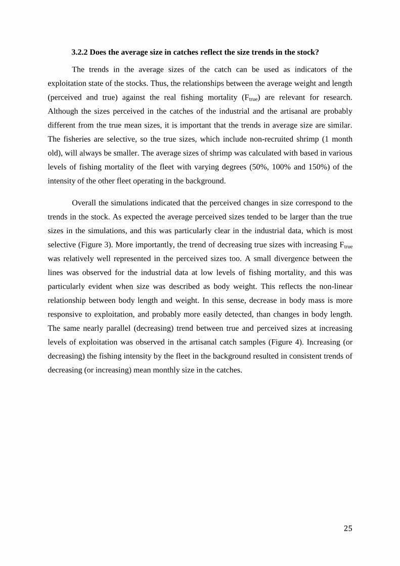
3.2.2 Does the average size in catches reflect the size trends in the stock?

The trends in the average sizes of the catch can be used as indicators of the

exploitation state of the stocks. Thus, the relationships between the average weight and length

(perceived and true) against the real fishing mortality (Ftrue) are relevant for research.

Although the sizes perceived in the catches of the industrial and the artisanal are probably

different from the true mean sizes, it is important that the trends in average size are similar.

The fisheries are selective, so the true sizes, which include non-recruited shrimp (1 month

old), will always be smaller. The average sizes of shrimp was calculated with based in various

levels of fishing mortality of the fleet with varying degrees (50%, 100% and 150%) of the

intensity of the other fleet operating in the background.

Overall the simulations indicated that the perceived changes in size correspond to the

trends in the stock. As expected the average perceived sizes tended to be larger than the true

sizes in the simulations, and this was particularly clear in the industrial data, which is most

selective (Figure 3). More importantly, the trend of decreasing true sizes with increasing Ftrue

was relatively well represented in the perceived sizes too. A small divergence between the

lines was observed for the industrial data at low levels of fishing mortality, and this was

particularly evident when size was described as body weight. This reflects the non-linear

relationship between body length and weight. In this sense, decrease in body mass is more

responsive to exploitation, and probably more easily detected, than changes in body length.

The same nearly parallel (decreasing) trend between true and perceived sizes at increasing

levels of exploitation was observed in the artisanal catch samples (Figure 4). Increasing (or

decreasing) the fishing intensity by the fleet in the background resulted in consistent trends of

decreasing (or increasing) mean monthly size in the catches.

26

Figure 3: Perceived and true sizes from size composition analysis of the industrial data at different levels of real

fishing mortality of this fleet. In this scenario no seasonal closures are implemented and the artisanal background

was set a 100%.

Figure 4: Perceived and true sizes from size composition analysis of the artisanal data at different levels of real

fishing mortality of this fleet. In this scenario no seasonal closures are implemented and the industrial

background was set a 100%.

0

5

10

15

20

25

30

0.00 0.20 0.40 0.60 0.80 1.00 1.20

Ftrue (month-1)

g/

mm

Weight&length Perceived+ True weight&length of shrimpVS Ftrue ( full strength artisanal)

WEIGHT PERCEIVED

LENGTH PERCEIVED

TRUE WEIGHT

TRUE LENGTH

0

5

10

15

20

25

30

0.00 0.20 0.40 0.60 0.80 1.00 1.20

g/

mm

Ftrue (month-1)

Weight&length Perceived+ True weight&length of shrimpVS Ftrue ( full strength industrial)

WEIGHT PERCEIVED

LENGTH PERCEIVED

TRUE WEIGHT

TRUE LENGTH

27

3.3. Scenarios

3.3.1. Scenario 1: Non-restricted fisheries.

The first scenario is a reference situation, and coarsely represents the fishery taking

place until about 1990 [9] when there were no restrictions on fleet sizes and operation time. In

the first set of simulations the industrial effort was varied continuously at three background

levels of the small-scale fishing intensity. In this case the yield curve for the industrial fleet

was monotonically rising (non-asymptotically) with increasing effort (number of vessels), a

reflection of the constant recruitment approach of the model. Under status quo (60 trawlers x

5000h; 4000 beach-seines x 200 days) the yield of the industrial fleet approached 6000 tons

and that of the artisanal fleet 1500 tons (Figures 5.1 and 5.3). With this number of vessels the

industrial fishery is largely unprofitable (annual deficit about $21 million) (Figure 5.2);

reduction of effort to 30 trawlers would reduce the total yield by only about 1000 tons, but

bring this fleet to a break-even of costs and revenues. Reduction of the small-scale fleet by

50% would increase the yields of the industrial fleet by about 1300 tons but still not make it

profitable in the long run (average deficit $ 12.5 million). The maximum economic yield of

the industrial fleet is achieved with a drastic reduction to about 12 trawlers. At status quo the

total fishing mortality (Ftrue) reaches 0.73.month-1

, and the average carapace length (CxL) in

the industrial catches is 25.5 mm. Reduction of the small-scale effort by 50% would bring the

F slightly down to 0.66 and have negligible influence on the size of the shrimp caught by the

industrial fleet (25.6 mm).

In the second set of simulations the small-scale effort was varied continuously at

discrete levels of the industrial fleet, representing a strong control on the later fleet. The

patterns observed followed largely a non-asymptotic curve as that observed for the industrial

fleet with regards to yield. At status quo the small-scale fleet was somewhat unprofitable (- $

6.7 million, divided by 4000 units) (Figure 5.4). It must be borne in mind that this figure

disregards the revenues brought by fish other than shrimps and small pelagics. Break-even

could be achieved by either reducing the small-scale fleet to 3400 beach-seines or bringing

the industrial fleet down by 50%, which would shoot the yield of shrimp of the small-scale

fleet to 2450 tons. The maximum economic yield for the small-scale fleet is achieved at about

1000 beach-seines, a drastic reduction as well. This represents the loss of many thousand full-

time and part-time jobs associated with the excess 3000 fishing units. At status quo the

average size of shrimps is 23.2 mm CxL and that of shad 11.0 cm TL. Also in the status quo

28

situation the average annual catch of small pelagics by the small-scale fleet is about 48150

tons, and the corresponding by-catch by the industrial fleet 3315 tons.

Figure 5.1 Figure 5.2

Figure 5.3 Figure 5.4

0

1000

2000

3000

4000

5000

6000

7000

8000

9000

5 15 25 35 45 55 65 90

To

nn

es

No vessels

Industrial shrimp yield average

100%art

50% art

-70000

-60000

-50000

-40000

-30000

-20000

-10000

0

10000

20000

30000

5 15 25 35 45 55 65 90

K$

No vessels

Industrial profit average 100% art

50% art

150% art

0

1000

2000

3000

4000

5000

6000

7000

8000

9000

0 1000 2000 3000 4000 5000 6000 7000 8000

To

nn

es

No Boats

Artisanal shrimp yield average

100% ind

50% ind

150% ind

-70000

-60000

-50000

-40000

-30000

-20000

-10000

0

10000

20000

30000

0 1000 2000 3000 4000 5000 6000 7000 8000

K$

No Boats

Artisanal profit average ( shrimp+shad)

100% ind

50% ind

150% ind

Figure 5. Scenario 1

29

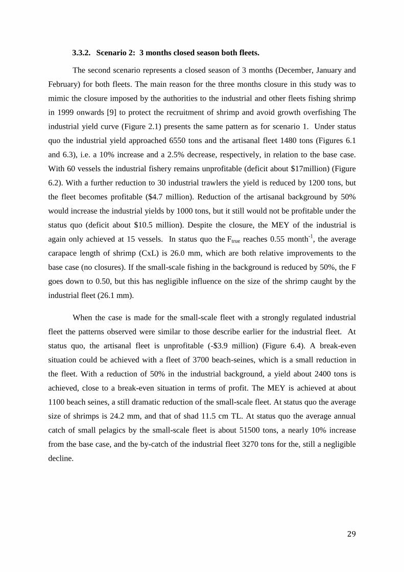
3.3.2. Scenario 2: 3 months closed season both fleets.

The second scenario represents a closed season of 3 months (December, January and

February) for both fleets. The main reason for the three months closure in this study was to

mimic the closure imposed by the authorities to the industrial and other fleets fishing shrimp

in 1999 onwards [9] to protect the recruitment of shrimp and avoid growth overfishing The

industrial yield curve (Figure 2.1) presents the same pattern as for scenario 1. Under status

quo the industrial yield approached 6550 tons and the artisanal fleet 1480 tons (Figures 6.1

and 6.3), i.e. a 10% increase and a 2.5% decrease, respectively, in relation to the base case.

With 60 vessels the industrial fishery remains unprofitable (deficit about $17million) (Figure

6.2). With a further reduction to 30 industrial trawlers the yield is reduced by 1200 tons, but

the fleet becomes profitable ($4.7 million). Reduction of the artisanal background by 50%

would increase the industrial yields by 1000 tons, but it still would not be profitable under the

status quo (deficit about $10.5 million). Despite the closure, the MEY of the industrial is

again only achieved at 15 vessels. In status quo the Ftrue reaches 0.55 month-1

, the average

carapace length of shrimp (CxL) is 26.0 mm, which are both relative improvements to the

base case (no closures). If the small-scale fishing in the background is reduced by 50%, the F

goes down to 0.50, but this has negligible influence on the size of the shrimp caught by the

industrial fleet (26.1 mm).

When the case is made for the small-scale fleet with a strongly regulated industrial

fleet the patterns observed were similar to those describe earlier for the industrial fleet. At

status quo, the artisanal fleet is unprofitable (-$3.9 million) (Figure 6.4). A break-even

situation could be achieved with a fleet of 3700 beach-seines, which is a small reduction in

the fleet. With a reduction of 50% in the industrial background, a yield about 2400 tons is

achieved, close to a break-even situation in terms of profit. The MEY is achieved at about

1100 beach seines, a still dramatic reduction of the small-scale fleet. At status quo the average

size of shrimps is 24.2 mm, and that of shad 11.5 cm TL. At status quo the average annual

catch of small pelagics by the small-scale fleet is about 51500 tons, a nearly 10% increase

from the base case, and the by-catch of the industrial fleet 3270 tons for the, still a negligible

decline.

30

Figure 6.1 Figure 6.2

Figure 6.3 Figure 6.4

0

1000

2000

3000

4000

5000

6000

7000

8000

9000

0 10 20 30 40 50 60 70 80 90 100

To

nn

es

No vessels

Industrial shrimp yield average

100% art

50% art

150% art

-70000

-60000

-50000

-40000

-30000

-20000

-10000

0

10000

20000

30000

0 10 20 30 40 50 60 70 80 90 100

K$

No vessels

Industrial profit average 100% art

50% art

150% art

0

1000

2000

3000

4000

5000

6000

7000

8000

9000

0 1000 2000 3000 4000 5000 6000 7000 8000

To

nn

es

No boats

Artisanal shrimp yield average

100% ind

50% ind

150% ind

-70000

-60000

-50000

-40000

-30000

-20000

-10000

0

10000

20000

30000

0 1000 2000 3000 4000 5000 6000 7000 8000

K$

No boats

Artisanal profit average ( shrimp+shad)

100% ind

50% ind

150% ind

Figure 6. Scenario 2

31

3.3.3. Scenario 3: six months closed season for the industrial fleet, two months

for artisanal fleet.

In this scenario, the recommendations of Masquine [23] were taken into account. A

closure from September to February for the industrial fleet was established, and for the

artisanal fleet from May and June. This author suggested adapting the closures of the artisanal

fleet to the rainy seasons, which it would allow for a combination of fishing and agriculture.

The industrial yield showed the same pattern as in earlier scenarios, i.e. a monotonically

rising curve with increasing the effort. Under the status quo, the yield obtained was close to

5600t, while the artisanal reached 2250t (Figure 7.1 and 7.3), a decrease of 6.5% and an

increase of 50% over the base cases, respectively. In this scenario, the industrial fleet shows

to be highly unprofitable (deficit close to $23 million) (Figure 7.2). With a reduction of the

effort up to 30 trawlers, the total yield would reduce to 4400t, and the fleet would be close to

break-even (deficit of $1 million). When a reduction of 50% is applied to the small-scale fleet

in the background, the total industrial yield gains 1200t, but the fleet is still non-profitable

(deficit of $15 million). The MEY for the industrial fleet is obtained with 12 vessels, a

dramatic reduction of the fleet. A total fishing mortality of 0.41month-1

is achieved at the

status quo, which is a marked reduction, and the CxL in the industrial catches rises 26.0 mm.

This is a larger shrimp size in the present model (L∞= 31 mm CxL), close to the modeled

spawning size (L50=26.7 mm CxL). The reduction by 50% of the artisanal fleet would reduce

the value of Ftrue to 0.35month-1

and the size of shrimp would be 26.2mm, a negligible

influence.

When the situation is analyzed from the artisanal perspective, at status quo the fishery

showed to be close to a break-even situation, with a deficit of only $2 million (Figure 7.4).

With a small reduction of 300 beach-seines the break-even situation is achieved. This can also

be achieved by reduction of the industrial strength by 50%, which would also result in an

increase of the artisanal shrimp yield of 800t. The MEY for this fleet is obtained at 1000

beach-seines, a dramatic change. At status quo, the CxL of shrimps caught by the small-scale

fleet is 22.8mm. and the length of shad is 11.4 cm TL. In this situation the catches of shad

would be situated around 52300t and the by catch by the industrial fleet at 2590t. These are

more favorable situations for both fleets.

32

Figure 7.1 Figure 7.2

Figure 7.3 Figure 7.4

0

1000

2000

3000

4000

5000

6000

7000

8000

9000

0 10 20 30 40 50 60 70 80 90 100

To

nn

es

No vessels

Industrial shrimp yield average

100% art

50% art

150% art

-70000

-60000

-50000

-40000

-30000

-20000

-10000

0

10000

20000

30000

0 10 20 30 40 50 60 70 80 90 100

K$

No vessels

Industrial profit average

100% art

50% art

150% art

0

1000

2000

3000

4000

5000

6000

7000

8000

9000

0 1000 2000 3000 4000 5000 6000 7000 8000

To

nn

es

No boats

Artisanal shrimp yield average

100% ind

50% ind

150% ind

-70000

-60000

-50000

-40000

-30000

-20000

-10000

0

10000

20000

30000

0 1000 2000 3000 4000 5000 6000 7000 8000

To

nn

es

No Boats

Artisanal profit average ( shrimp+shad)

100% ind

50% ind

150% ind

Figure 7. Scenario 3

33

3.3.4. Scenario 4: Six months closed season for the industrial fleet and non-

restricted fishery for the artisanal fleet.

This scenario explores the management measures that can realistically be applied to

both fleets. Under status quo this scenario penalizes the industrial fleet that sees the shrimp

yield reduced to 5000t, but greatly benefit the small-scale fleet, which achieves a shrimp yield

of 2800t (Figures 8.1 and 8.3). The industrial fleet becomes highly unprofitable, with a deficit

of about $26 million (Figure 8.2). With a reduction of the industrial fleet to 30 vessels it

would still remain unprofitable (deficit $4 million), with their total yield reduced by 1100t.

The estimated point for a break-even is situated in 21 trawlers, which is a number lower than

obtained under previous scenarios. If the artisanal background is reduced by 50%, total

industrial yields would increase in 1400t, but the fleet would still remain unprofitable (deficit

of $17 million). Under this regime the MEY for the industrial fleet is achieved with 10

vessels, a tremendous reduction in effort. At status quo the total fishing mortality reduces to a

reasonable value of 0.43month-1

, and the average carapace length increases to 26.3mm CxL in

the industrial catches. If a reduction of 50% is imposed on the artisanal fishery background,

the Ftrue is further reduced to 0.36 and the average length in the industrial catches increases to

26.5 mm, very close to the maturation size.

From the artisanal fleet point of view the status quo is only slightly unprofitable

(deficit $0.5 million) (Figure 8.4). The break-even situation could be achieved reducing less

than 100 beach-seines. With a reduction by 50% of the industrial background, the total yield

of shrimp obtained by the artisanal could greatly increase to above 3550t. The MEY is

achieved at 1000 beach seines, still a drastic reduction of the fleet. At status quo the average

size of the shrimps in the beach seines is 23.0mm of carapace length, still far below the

maturation size of shrimp and that of the shad is 11.3 cm TL. Under this restrictive scenario

for the industrial fishery the annual catches of small pelagics by the small-scale fleet would

rise to about 52800t and the by-catch by the industrial fleet decline to 1350t.

34

Figure 8.1 Figure 8.2

Figure 8.3 Figure 8.4

0

1000

2000

3000

4000

5000

6000

7000

8000

9000

0 10 20 30 40 50 60 70 80 90 100

To

nn

es

No Vessels

Industrial shrimp yield average

100% art50% art150% art

-70000

-60000

-50000

-40000

-30000

-20000

-10000

0

10000

20000

30000

0 10 20 30 40 50 60 70 80 90 100

K$

No Vessels

Industrial profit average

100%art50% art

0

1000

2000

3000

4000

5000

6000

7000

8000

9000

0 1000 2000 3000 4000 5000 6000 7000 8000

To

nn

es

No boats

Artisanal shrimp yield average

100% ind

50% ind

150% ind

-70000

-60000

-50000

-40000

-30000

-20000

-10000

0

10000

20000

30000

0 1000 2000 3000 4000 5000 6000 7000 8000

K$

No Boats

Artisanal profit average ( shrimp+shad)

100% ind

50% ind

150% ind

Figure 8. Scenario 4

35

3.3.5. Scenario 5: Closed season of six months for industrial fleet, and one month

for artisanal fleet.

The fifth scenario analyzed mimics the current situation in the North Sofala bank,

where a closed season from October to March is applied to the industrial fleet and a closure of

one month, January, is applied to the artisanal fleet. The yield curve for the industrial fleet

follows previous patterns, and status quo the total industrial yield declines to 5200t, with an

increase for the artisanal fleet to above 2600t (Figures 9.1 and 9.3). This situation is still

highly unprofitable for the industrial fleet (deficit about $24.5 million) (Figure 9.2). A one-

sided reduction of industrial effort to 30 vessels would reduce this deficit to an annual average

of $3 million in the long run. The yield would also decrease to 4000t. The MEY of the

industrial fleet with unchanged artisanal fleet in the background is achieved with 12 trawlers,

a drastic reduction once more. At status quo the Ftrue reaches 0.42month-1

and the shrimp

average CxL is 26.4 mm. If a reduction by 50% in the artisanal background is realized, this

would bring the total fishing mortality to 0.36month-1

, almost a negligible influence, but the

size of shrimp caught by the industrial fleet (26.5 CxL mm) would approach the maturation

size in this model.

At status quo the artisanal fleet is close to a break-even situation (deficit $0.3 million)

(Figure 9.4). The break-even situation can be achieved with a soft reduction of 100 beach-

seines, or bringing down the industrial fleet by 50%, which would result on an increase of

catches by the artisanal fleet of 700t. Otherwise, the MEY is achieved at about 1000 beach-

seines, a high and drastic reduction of the fleet. At status quo, the average size of shrimps is

23.3mm and the shad is 11.3 cm TL in the catches of the beach-seines. Also in status quo, the

catches of small pelagics by the artisanal fleet are 54000t and the by-catch by the industrial

fleet is further reduced to 1450t.

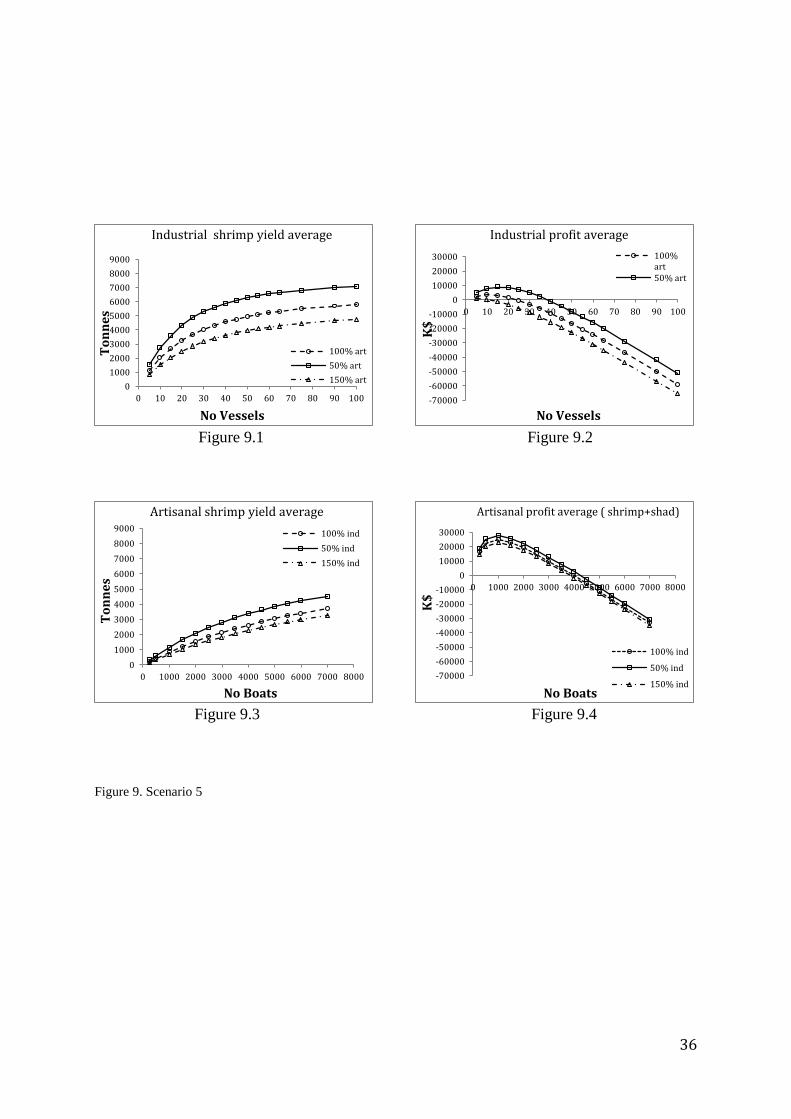
36

Figure 9.1 Figure 9.2

Figure 9.3 Figure 9.4

0

1000

2000

3000

4000

5000

6000

7000

8000

9000

0 10 20 30 40 50 60 70 80 90 100

To

nn

es

No Vessels

Industrial shrimp yield average

100% art

50% art

150% art

-70000

-60000

-50000

-40000

-30000

-20000

-10000

0

10000

20000

30000

0 10 20 30 40 50 60 70 80 90 100

K$

No Vessels

Industrial profit average

100%art50% art

0

1000

2000

3000

4000

5000

6000

7000

8000

9000

0 1000 2000 3000 4000 5000 6000 7000 8000

To

nn

es

No Boats

Artisanal shrimp yield average

100% ind

50% ind

150% ind

-70000

-60000

-50000

-40000

-30000

-20000

-10000

0

10000

20000

30000

0 1000 2000 3000 4000 5000 6000 7000 8000

K$

No Boats

Artisanal profit average ( shrimp+shad)

100% ind

50% ind

150% ind

Figure 9. Scenario 5

37

3.3.6. Scenario 6: Closed season of six months for industrial fleet, and two month

for artisanal fleet.

The sixth scenario analyzed mimics the current situation in the South Sofala bank,

where, in addition to the usual closed season from October to March for the industrial fleet, a

closure in January and February is applied to the artisanal fleet. The yield curve for the

industrial fleet presents a recurrent pattern, and in status quo the yield achieved by the

industrial fleet is above 5600t and that of the artisanal fleet is 2300t (Figures 10.1 and 10.3).

With 60 vessels, the industrial fleet is largely unprofitable (deficit close to $22 million)

(Figure 10.2); a reduction of 50% of the industrial fleet would reduce the total yield by 1200t,

but bring this fleet to an almost break-even situation (deficit $0.7 million). If a reduction by

50% in the artisanal background is implemented the industrial yields increase by 1200t, but

would still remain far from profitable (deficit of $14 million). The MEY of the industrial fleet

is achieved at 12 vessels, a dramatic reduction of the fleet. At status quo the total fishing

mortality is 0.41month-1

and the shrimp average length catches by the industrial fleet is

26.4mm. The reduction of 50% in the artisanal background has negligible influence in the

(0.35month-1

) and average length (26.5) of shrimp.

Despite the imposition of a two month closure, at status quo the small-scale sector is

close to a break-even situation (deficit of $0.4 million) (Figure 10.4). The break-even could

be achieved with just a reduction of 100 beach-seines, or reducing the industrial strength by

50%. This would boost the yield of the shrimp of the artisanal fleet to 3100t. The MEY is

achieved at about 1000 beach-seines, again a drastic reduction, that represents the loss of

many jobs associated with the excess of 3000 fishing units. At status quo, the shrimp size is

23.8 mm and the shad 11.6 cm TL in the beach-seines. Also at status quo, the average annual

catch of small pelagics is 54400t and the industrial by-catch is 1800t, which are still very

favorable situations for both fleets.

38

Figure 10.1 Figure 10.2

Figure 10.3 Figure 10.4

0

1000

2000

3000

4000

5000

6000

7000

8000

9000

0 10 20 30 40 50 60 70 80 90 100

To

nn

es

No Vessels

Industrial shrimp yield average

100% art

50% art

150% art

-70000

-60000

-50000

-40000

-30000

-20000

-10000

0

10000

20000

30000

0 10 20 30 40 50 60 70 80 90 100

K$

No Vessels

Industrial profit average

100% art

50% art

150% art

0

1000

2000

3000

4000

5000

6000

7000

8000

9000

0 2000 4000 6000 8000

To

nn

es

No Boats

Artisanal shrimp yield average

100% ind

50% ind

150% ind

-70000

-60000

-50000

-40000

-30000

-20000

-10000

0

10000

20000

30000

0 1000 2000 3000 4000 5000 6000 7000 8000

K$

No Boats

Artisanal profit average ( shrimp+shad)

100% ind

50% ind

150% ind

Figure 10. scenario 6

39

4. Discussion

This is one of the first attempts to apply two-fleet two-prey fishery models for

management purposes. The model itself is still under development, and there is ample room

for improvement. Further modifications of the model aim to achieve higher ecological detail.

The present version contemplates, however, a very large spectrum of possibilities with regard

to the fish biology and ecology, fleet operation, economics and management measures. This

version of model was considered sufficiently flexible to address the main research questions

raised with an acceptable degree of detail and robustness. An additional challenge was to

populate the model with appropriate statistics and parameters to describe the real situation in

the Sofala Bank. Again, the values utilized were those that could be estimated from the

literature or Mozambican statistics, and often from very limited field surveys, or otherwise

figures that seemed to be appropriate by the authors. A major limitation is the difficulty to

simulate fisher’s behaviour. For instance, it is a known fact that industrial enterprises in

Mozambique tend (or attempt) nowadays to concentrate their fishing effort at the start of the

fishing season because of high catch rates. However, it is impossible to say whether that

behaviour is a cause for the present closure regulation or a consequence of it. Would fishers

still behave like that if the resource was abundant and there were no closures? Considerations

of fishers’ behaviour are for similar reasons seldom dealt with in system models like the

present one, rather investigated in agent-based models.

4.1. Does the original model describe the current situation in a

satisfactory way? Do the model result mimic trends observed in the

fishery?

As it was stated in the introduction “the goal of this study is to develop a set of simple

and simulation scenarios that can be useful for management orientation. These scenarios

should be realistic and investigate conflicts between industrial and small scale fisheries”.

There are only few points of reference to judge whether or not the present simulations

have a realistic grounding. An obvious benchmark is the total yield obtained by the two fleets

under the different management regimes. The 1st scenario designed to be used as a reference

was a non-restricted fishery tries to mimic the situation in the Sofala Bank until the 1990 [9].

The official reports [9] reported an industrial catches of shrimp about 6000 tonnes, while the

results obtained in the model for status quo showed a catches identical, about 6000 tonnes.

40

Reports of catches from the 90’s of the small-scale fisheries are inexistent, but this problem it

is still present in the last reports [6], where the official information talks about “estimation of

catches from the artisanal fleet”. With these limitations in mind, and assuming that the

reports of industrial catch correspond to their actual catches, it seems that this scenario can be

appropriately utilized as a reference.

The 2nd

scenario, with a closed season of 3 months mimics the situation from 1990

onwards [9] until the late 2000’s. The industrial catches from the official reports showed a

range of yields from 6500 to 8500t (1990-2002). The model obtained 6500 for the status quo,

but it must be borne in mind that, according to official statistics, 80 industrial vessels were

operative on average in that period. The same unresolved situation applies in this period with

regard to artisanal statistics. The situation occurring from the late 2000’s to the present is

probably depicted more approximately in scenario 4, with a 6 months closure for the

industrial fleet. This would bring their predicted long-term yield down to about 5000 tons,

against the reported 4200 tons in 2011, reflecting the expected trend. So, it seems that in

general there is some correspondence between the yields expected from the model and those

obtained historically in similar management regimes.

The profitability of the industrial fishery could also be a means to benchmark the

model. After all, a capitalized fishery would not tolerate to operate in deficit conditions for a

long time, so what we observe in status quo can be an industrial fleet in breakeven conditions,

a probable long-term equilibrium. In this sense the model does not seem to perform well as it

indicates an industrial fishery in recurrent deficit. At least two reasons can explain this. First,

the information about the first-hand prices of shrimp is largely contradictory. Immediately

after the western financial crisis in 2008, and partially owing to great competition from

aquaculture, the price of Mozambican wild shrimp plunged to about $6 / kg according to

many independent sources [44] following the trend in the world markets. This is the kind of

price level that was used in the present simulations (although with a correction for shrimp

size). But, as late as in 2012 the Institute of Fisheries Research in Mozambique (IIP) was still

using a base price of $9 /kg in their bio-economic simulations. This difference alone would

bring the profitability curves of the fishery (e.g. Figure 2.2 or 4.2) upwards at status quo by

$15 million, which is close to break-even conditions. Secondly, in the present simulation the

current street prices for diesel ($1/l) were utilized. The IIP uses instead a price of ($0.75/l)

that reflects the fuel exemption given by the State to the industrial fleet. In the present model

fuel costs are taken to represent 60% of the variable costs of the trawlers, so that the fuel

41

subsidy decreases total variable costs by 15%. The consequence of this is to push the

profitability curves upwards and the MEY point further to the right, towards higher fishing

intensity (e.g. more vessels). Lastly, after a lasting shock to the industry the trawler fleet in

Mozambique seems to be operating in 2013 with about 30 vessels. This corresponds

approximately to the break-even situation predicted in the present model at status quo (Figure

2.2), and gives an indirect indication that the present predictions may indeed be realistic, but

more so in the present times than in 2008-2009.

4.2. How do the different management controls in isolation impact on

the fisheries?

Sensitivity analyses were utilized to understand the isolated effect of different controls on

yield, profit and size of the shrimp on each fleet at the time. The management control that

presented a higher impact was the size of shrimp at first catch (L50) for the industrial yield,

with a reduction of 25% of the yield when size is increased by 10%. Otherwise, the same

control did not affect, or in a very small proportion the artisanal yield. The measure that

affected the most the artisanal fisheries was the reduction of the effort, with a 7% decrease in

the artisanal yield for a change of -10% in effort. All these trends suggest that at status quo

the shrimp fishery is tightly connected between the two fishing fleets. Decrease in fishing

pressure in one fleet leads to loss in that fleet, with compensatory gain in the other fleet, a

competitive situation. Introduction of simultaneous closures for the two fleets had some

expected and some unexpected effects: the average size of shrimp in the catches increased,

the yields of the industrial fleet increased, but the yields of the small-fleet decreased. Both

fleets became less profitable, and this was particularly evident for the small-scale fleet, if the

closure took place in January, which is in their more productive season. Thus, and as

expected, the introduction of closures has some biological effects, somewhat more

pronounced in January, but its main result is making the fleets less profitable.

4.3. What inaccuracies are brought to the stock assessment if the capture

of the artisanal fleet is not taken into account?

4.3.1. Perception by research: Fishing mortality

There are two major reasons to explain the difference between Ftrue from Fperceived at

any fishing intensity of one of the fleets, with the Fperceived overestimating Ftrue. One reason is

sampling bias and the other is stochasticity. Estimations of the average F across age groups

42

from industrial catch data alone would in principle correctly provide the full F (small-scale +

industrial), but only for the older age groups. The estimates from the industrial data omit the

lower F inflicted by the small scale fleet on the younger age groups. Thus, even if the average

Ftrue is lower than the Fperceived in the older cohorts it applies cumulatively along a longer part

of the life-cycle and becomes dominant. Experiments with the model showed that when the

small-scale fleet exploits three age groups more than the industrial fleet the cumulative Ftrue is

on average 11% larger than the cumulative Fperceived from the industrial data; along a full life

of a cohort this can lead to a 33% overestimate of the number of survivors in a cohort

reaching the last age-group in the fishery (i.e. the sequential fishery). This error affects the

data obtained from the industrial fleet, but not so seriously the data from the small-scale fleet,

which (in this model) operates un-selectively, catching big and small shrimp. Another

consequence of this fishing pattern is that the deviation between Fperceived in the industrial data

and Ftrue increases with the fishing intensity of the industrial fleet (Figure 1).

The second source of error, which superimposes on the first one, is the error

introduced by uncertainty (stochasticity) in the model. In an experiment with model the log-

normal nature of the assessment error (CV=10%) alone increased the Fperceived by about 4% in

relation to the Ftrue. Unlike the first source of error, this over-estimation of Fperceived in the data

from the small-scale fleet seems to be additive along the range of Ftrue as the two lines run

parallel (Figure 2). In conclusion, sampling only the size-composition of shrimp captured by

the industrial fleet bias the estimates the fishing mortality. The error induced by sampling the

size/age distribution of the industrial catch alone may be partially compensated by the

inherent error in assessment, at least in the conditions utilized in the present model. As the

sampling bias dominates the error, this calls for good sampling of catches of both fleets.

However, the over-estimation of recruit survival in real conditions does not seem to be

exceedingly serious.

4.3.2. Perception in size of capture shrimp

The values of sizes presented for the shrimp captures, true and perceived values,

showed to be different, although following the same pattern among all the scenarios. There

were not changes in the trends described in sizes among scenarios of the industrial fleet and

the small-scale fisheries. The difference between perceived and true values at any fishing

intensity of one of the fleets it is due to the sampling method used. In fact, the values use for

the official assessments are taking only into account the perceived values , that means the data

43

comes only from the catches of the industrial fleet. The trawlers are only exploiting one part

of the total stock, it can be said somehow that they are selective, fishing the bigger shrimps of

the stock; meanwhile, the small-scale fisheries are not selective, and therefore are catching

any size of shrimp. Therefore, this difference is depicted in the appendix I-XII, where the

perceived size trends present higher values than the true size trends. In conclusion, using the

average size of the shrimp from the catches of the industrial fleet (perceived sizes) as

indicator of the state of the stock can be slightly bias, because the size of the stock is

declining faster what it is observed in the catches of the true values, but they don’t see to be

extremely differences (average of 7mm CxL for industrial fleet and 6mm for the small-scale

fisheries). That would bring inaccuracies to the stock assessment. One possible point of

concern is that the industrial trawlers, being more selective and mobile, can be un-

proportionally targeting the females, which grow faster and larger and are, thereby, more

valuable. This means that an increased fishing mortality may deplete faster the spawning

stock by two processes: selective catch of faster growing females at the beginning of the

season, closer to shore, and selective search for large shrimp (females) offshore later in the

season. The present model is too coarse to investigate the consequences of these patterns.

4.4. Are the same controls / technical measures justified for both fleets?

Analysing the overall of all the scenarios, at the status quo, the industrial fleet is never

profitable, and with a large deficit. Even reducing by 50% the artisanal background, still

keeps under deficit. Four out of six scenarios for the small-scale fisheries present at status

quo fisheries close to a break-even situation or with profits, and when the background is

reduced by 50%, these artisanal scenarios become in profits. Interestingly, and despite the

coarseness of the model, the present simulations repeatedly suggest that the best overall

economic efficiency can be achieved by regulating (decommissioning) strongly the industrial

fleet. At lower levels of effort than status quo the small-scale fleet, despite its primitive

character, could become very profitable, and compensate for the lost profit in the industrial

fleet. At present, however, the fisheries are working for different targets: the artisanal is

mostly a subsistence fishery (although it seems that for the last years the increase in catches

would mean that there is a market for them), and the industrial is exportation-oriented market.

44

4.5. Which management measure has more impact on the fishery in a

sector–wide approach?

All this different scenarios, working with closed seasons as a main management

control measure, are pulling towards a reduction in the effort, since the results have shown

that the fishery is not profitable for the industrial in the levels that is working now. The

results obtained can be perceived as expected, since the reports from the last years [7, 8, 9 and

10] showed a tendency to decrease inside the industrial fleet, but it is still complicated to give

a proper assessment due to the lack of official information to introduce the proper values in

the model. The change in the management strategy from scenario to scenario (different closed

seasons) does not result in large differences among them, but in terms of protection of stock

(mortality levels) has a large influence and it must be considered if that is the target

(biological approach). Reduction of effort in the both fleets will produce an increase in

profits, therefore in economic terms. But, dramatic reductions in the industrial fleet must just

to get a break-even situation, and in both fleets to achieved maximum economic yield. As

mentioned above, this may not be an interesting objective for the small-scale fleet.

4.6. How would the small-scale fisheries benefit from a reduction in the

by-catch of the industrial fleet?

In general lines, there is a direct relation between the increase of shad yields and

management measures reducing the activity of the industrial fleet. The scenarios applying

closed seasons depicted in average a 10% more of yield in the artisanal catches of shad than

in the 1st scenario, and therefore a higher profit. Always that the industrial fleet is reduced

somehow (fleet number or background), the yields for the artisanal shad catches increase and

consequently also decreases the by-catch of the industrial. But the shad does not represent all

the species of fish that can be found in the by-catch and in the gears of the small-scale

fisheries. The other species presents higher commercial values than the shad, and there it is

where the importance of the by-catch in terms of profit for the artisanal can make the

difference. The model does not contemplate these other species inside the parameters mostly

because there is a lack of biological information of them, but there is more information about

the shad. The aim of the model is to mimic the fishery in an easy way, trying to do not get

really complex and with the inclusion of these other fishes in the model, it should be included

also trophic chains, due to some of these species use the shad as feeding, and therefore the

model would acquire a complexity far from what it is intended in the development of this

model. For that reason, this study did not study in a deep way the shad situation.

45

5. Conclusions

The shrimp fishery in the Sofala bank offers a general and interesting

case-study of physical interactions between two fleets. A model was utilized to

develop scenarios similar to the real fishery, with a reasonable accuracy, despite some

uncertainty about prices and costs in the real fishery. Therefore an update of

parameters may be required, to represent the real situation in Sofala.

The fishing mortality and average size of shrimp perceived by research

in the industrial fishery alone are somewhat, but not dramatically, biased. Researchers

must be careful and check what it is happening in terms of shrimp size in the artisanal

as well to perform adequate assessments of the state of the stocks.

There is a direct competition between fleets: when effort is reduced in

one fleet, the other fleet obtains improved yield and profit. It is, thus, inappropriate to

manage the fleets separately. The fleets serve different people, markets and objectives.

This can be taken account in a preliminary design of management measures to the two

fleets.

The timing and extension of the closed seasons, a preferred technical

measured in Sofala, influences the levels of yields and profits. Closed seasons can be

adapted separately for each fleet and goal.

All the scenarios indicated that in order to maximize yield and profit in

the whole fishery in the long term, a strong reduction of fishing effort, must be

realized in the industrial fleet. The costs of decommissioning a great part of the fleet

must be analyzed, and can be introduced in a model of this type.

Seasonal closures achieve different levels of protection of the stock, but

probably do not address the economic problem of an oversized industrial fleet.

46

References

1. - Amire, A.V., Monitoring, measurement and assessment of fishing capacity: the Nigerian

experience, in FAO Fisheries Technical Paper 445. 2003. FAO: Rome- Italy.

2. - FAO., Fishery and Aquaculture Country Profiles. Cambodia (2011). Country Profile Fact

Sheets, in FAO Fisheries and Aquaculture Department [online]. Rome- Italy. 2011.

http://www.fao.org/fishery/facp/KHM/en. [Checked 4th August 2013]

3. - Gillett, R., Global study of shrimp fisheries, in FAO Fisheries technical paper 475. 2008.

FAO: Rome- Italy.

4. - Pinto, M.A., ed. Gear selectivity for three by-catch species in the shallow-water shrimp

trawl fishery at the Sofala Bank, Mozambique. 2011. WIOMSA Book Series 1. 489-506.

5. - Kelleher, V., Mussa, A. (1995). Retention of by-catch for human consumption; The

Mozambique experience., In Report and Proceedings of TCDC Workshop - Utilisation of by-

catch from Shrimp Trawlers, Madagascar, 6-8 June, 1995., Governement of Madagascar.

1995. FAO.

6. - Palha de Sousa, L., Abdula, S., Palha de Sousa, B., J. Penn, J., and D. Howell, D.,

Relatório Interno de Investigação Pesqueira no 16: O Camarão do Banco de Sofala 2012, in

Report Instituto Nacional de Investigação Pesqueira. 2012. p. 75.

7. - Ministério das Pescas, Recenseamiento da pesca artesanal 2007. Principais Resultados,

in IDPPE. 2009, Instituto de Desevolvimento de pesca a pequena escala. Maputo

Mocambique.

8. - NORAD - The Norwegian Agency for Development Cooperation – and ICEIDA –

Icelandic International Development Agency, Mid Term Review. Assistance to the Fisheries

Sector of Mozambique. Co-financed by Norway and Iceland (2009-2013). 2012. Final Report.

Revised July 2012.

9. - Sousa, L.P.d., et al., Research assessment for the management of the industrial shallow-

water multi-species shrimp fishery in Sofala Bank in Mozambique. Fisheries Research. 2006.

77 p.207-219.

47

10. - Menezes, A.M., The Governance of Natural Resources in Mozambique: Artisanal

Fishery. State University of New York, College of Environmental Science and Forestry.

2008: Syracuse, New York.

11. - Akande, G., Technologies for bycatch handling on board, transfer to shore, processing

and marketing. Nigerian Institute for Oceanography and Marine Research. 2002: Lagos,

Nigeria.

12. - Gillett, R., The marine fisheries of Cambodia. FAO/FishCode Review. 2004. FAO:

Rome- Italy. pp. 57.

13. - Funge-Smith, S., Lindebo, E. & Staples, D., Asian fisheries today: the production and

use of low value “trash fish” from marine fisheries in the Asia-Pacific region, in FAO

Regional Office for Asia and the Pacific. 2005: Bangkok, Thailand.

14. - Kelleher, K., Discards in the world’s marine fisheries–an update, in FAO Fisheries

Technical Paper 470. 2005. FAO: Rome- Italy.

15. - Lopes, S. and H. Gervasio, Co-Management of Artisanal Fisheries in Mozambique: a

Case Study of Kwirikwidge Fishing Centre, Angoche District, Nampula Province. ICLARM.

2003. p. 29.

16. - Santos, J., O papel da Administração Pesqueira na gestão do subsector artesanal em

Moçambique. O presente e modelos para o futuro. 2008. Direcao nacional de administracao

Pesqueira- Ministério das Pescas: p. 150.

17. - Momade, F.C. Credit for small scale fishery in Mozambique, in M.Sc. thesis. Norwegian

College of Fisheries Science. 2005, University of Tromsø: Norway.

18. - Jacquet, J.D., Zeller, D., National conflict and fisheries: Reconstructing marine fisheries

catches for Mozambique, 1950-2004. Fisheries Centre. The University of British Columbia.

2007. Working Paper Series: nº 2007-02.

19. - República de Moçambique, Lei das Pescas, in Lei nº 3/90. 1990. Boletim da República, I

Série, nº.39, de 26 de Setembro.

48

20. - Ministério das Pescas, Relatorio do 1 Semestre da Campana de Pesca 2007. Internal

report. Direcção Nacional de Administração Pesqueira ( DNAP). 2007. Maputo

Mocambique.

21. - Mualeque, D., Santos, J., Biology, fisheries and distribution of Thryssa vitrirostris

(Gilchrist & Thompson 1908) and other Engraulidae along the coast of the Sofala Bank,

western Indian Ocean. African Journal of Marine Science, 2011. 33(1): p. 127-137.

22. - Wilson J., Zitha J., Social, economic and environmental impact of beach seining in

Mozambique -draft report. 2007. FAO: Rome- Italy.

23. - Masquine, Z., Baloi, A.P, de Premegi, N. and Caputi, N., The artisanal fishery for

shrimp in Nampula and Zambezia Provinces of Mozambique for 1997-2002. Unpublished

Report. 2005, Instituto Nacional de Investigação Pesqueira: Maputo Mocambique.

24. - Haddon, M. 2001. Modelling and Quantitative Methods in Fisheries. Boca Raton, Fla:

Chapman & Hall/CRC.

25. - Franco, A.R., Ferreira, J.G. & Nobre, A.M. Development of a growth model for penaeid

shrimp. Aquaculture, 2006. 259(1–4) p. 268–277.

26. - Blackwood, J.C., Hastings, A., Mumby, P.J. A model-based approach to determine the

long-term effects of multiple interacting stressors on coral reefs. Ecological applications,

2011, 21(7) p. 2722-2733.

27. - Da Rocha, J.M., Gutierrez, J.M., Endogenous fishery management in a stochastic model:

Why do fishery agencies use TACs along with fishing periods? Environmental and Resource

Economics. 2012. Volume 53, Issue 1, p. 25-59.

28. - Skagen, D.W., Skern-Mauritzen, M., Dankel, D., Enberg, K., Kjesbu, O.S., A simulation

framework for evaluating fisheries management decisions using environmental information.

ICES Journal of Marine Science, 2013. 70(4) p. 743–754.

29. - Centro Inter-Americano para el Desarrollo de Ecosistemas Sustentables (ICSED),

Desarrollo de herramientas económicas para la preparación de políticas sostenibles en el

sector pesquero del Golfo de Honduras. Tomo I: Caracterización de las pesquerías de

49

camarón y angosta, aproximación conceptual para la gestión pesquera. PROARCA/CAPAS.

2000.

30. - Bacalso, R.T. The use of alternative scenarios from an ecosystem-based model

simulation of the Danajon bank municipal fisheries as input to evaluating fisheries

management objective in a choice experiment, in M. Sc. Thesis. Visayas Cebu College. 2007,

University of the Philippines.

31. - Pelgröm, H. & Sulemane, M. 1982. Regional and country developments: Mozambique,

in Fish by-catch... Bonus from the Sea. 1982. Ottawa: FAO/IDRC. p. 139–140.

32. – IDPPE: Projecto de recolha da fauna acompanhante em Quelimane: Análise da

informação recolhida pelos fiscais. 1994, Instituto de Desenvolvimento de Pesca de Pequena

Escala: Maputo Mocambique, p. 6–15.

33. - Clucas, I., A Study of the options for utilization of bycatch and discards from

marine capture fisheries. FAO Fisheries Circular, 1997.

34. - Santos, J. 2013. Sofala v4: a fisheries model of two competing fleets. Norwegian

College of Fisheries Science. Unpublished report. 2013, University of Tromsø: Norway.

35. - Tinley K.L., et al., Wildlife and wild places in Mozambique. Oryx, 1976. 13 (4): p. 344-

350.

36. - Ministério das Pescas, Assistance to the fisheries sector of Mozambique. Document of

the programme co-financed by Norway and Iceland. 2009, Yangula Estudos e Projectos Lda.,

Maputo Mocambique. p. 86.

37. - Quinn, G.P. , Keough, MJ., Experimental design and data analysis for biologists.

Cambridge University Press: Cambridge. 2002.

38. - Walters, C.J. , Martell, S., 2004. Fisheries Ecology and management. Princeton

University Press. 2004. p. 448.

39. - Hamby, D.M., A review of techniques for parameter sensitivity analysis of

environmental models. Environmental Monitoring and Assessment. 1994. 32 (2): p. 135-154.

50

40. - Jager, HI., King, AW., Spatial uncertainty and ecological models. Ecosystems, 2004. 7:

p. 841-847.

41. - Cariboni, J., Gatelli, D., Liska, R., Saltelli, A., The role of sensitivity analysis in

ecological modelling. Ecological Modelling, 2006. 203: p. 167-182.

42. - Kleijnen, J.P., An overview of the design and analysis of simulation experiments for

sensitivity analysis. European Journal of Operational Research, 2004. 164: p. 287-300.

43. - Mitcheson, Y.S., Biology and Ecology Considerations for the Fishery Manager.

Chapter 2 in Cochrane and Garcia (eds) A Fishery Manager’s Guidebook. 2009.

44.- www.macauhub.com.mo : “Autoridades de Moçambique procuram Mercado alternativo

para o camarão”. http://www.macauhub.com.mo/pt/2009/06/30/7319/. [Checked 28th

november 2013].

I

Appendix

Scenario 1: Non-restricted fishery. INDUSTRIAL

0.00

0.20

0.40

0.60

0.80

1.00

1.20

1.40

0 10 20 30 40 50 60 70 80 90 100

F (

mo

nth

-1)

No Industrial Vessels

Fperceived VS. Ftrue (full strength artisanal)

F PERCEIVED

F TRUE

0.00

0.20

0.40

0.60

0.80

1.00

1.20

1.40

0 10 20 30 40 50 60 70 80 90 100

F (

mo

nth

-1)

No Industrial Vessels

Fperceived VS. Ftrue (50%artisanal)

0.00

0.20

0.40

0.60

0.80

1.00

1.20

1.40

0 10 20 30 40 50 60 70 80 90 100

F (

mo

nth

-1)

No Industrial Vessels

Fperceived VS. Ftrue (150%artisanal)

0

5

10

15

20

25

30

0.00 0.20 0.40 0.60 0.80 1.00 1.20

Ftrue ( month-1)

gr/m m

Weight&length Perceived+ True weight&length of shrimp VS Ftrue( full strength artisanal)

WEIGHT PERCEIVED

LENGTH PERCEIVED

TRUE WEIGHT

TRUE LENGTH

0

5

10

15

20

25

30

0.00 0.20 0.40 0.60 0.80 1.00 1.20

gr/

mm

Ftrue ( month-1)

Weight&length Perceived VS Ftrue ( 50% artisanal)

0

5

10

15

20

25

30

0.00 0.20 0.40 0.60 0.80 1.00 1.20

gr/

mm

Ftrue ( month-1)

Weight&length Perceived VS Ftrue ( 150% artisanal)

II

Scenario 1: Non-restricted fishery. ARTISANAL

0.00

0.20

0.40

0.60

0.80

1.00

1.20

1.40

0 1000 2000 3000 4000 5000 6000 7000 8000

F (

mo

nth

-1)

No Artisanal boats

Fperceived VS. Ftrue (full strength industrial)

F PERCEIVED

F TRUE

0.00

0.20

0.40

0.60

0.80

1.00

1.20

1.40

0 1000 2000 3000 4000 5000 6000 7000 8000

No Artisanal Boats

Fperceived VS. Ftrue (50% industrial)

0.00

0.20

0.40

0.60

0.80

1.00

1.20

1.40

0 1000 2000 3000 4000 5000 6000 7000 8000

No Artisanal Boats

Fperceived VS. Ftrue (150% industrial)

0

5

10

15

20

25

30

0.00 0.20 0.40 0.60 0.80 1.00 1.20

g/

mm

Ftrue

Weight&length Perceived+ True weight&length of shrimp VS Ftrue( full strength industrial)

WEIGHT PERCEIVED

LENGTH PERCEIVED

TRUE WEIGHT

TRUE LENGTH

0

5

10

15

20

25

30

0.00 0.20 0.40 0.60 0.80 1.00 1.20

g/

mm

Ftrue

Weight&length Perceived VS Ftrue ( 50% industrial)

0

5

10

15

20

25

30

0.00 0.20 0.40 0.60 0.80 1.00 1.20

g/

mm

Ftrue

Weight&length Perceived VS Ftrue ( 150% industrial)

III

Scenario 2: Closed season of 3 months for both fleets. INDUSTRIAL

0.00

0.20

0.40

0.60

0.80

1.00

1.20

1.40

0 10 20 30 40 50 60 70 80 90 100

F (

mo

nth

-1)

No Industrial vessels

Fperceived VS. Ftrue (full strength artisanal)

F PERCEIVED

F TRUE

0.00

0.20

0.40

0.60

0.80

1.00

1.20

1.40

0 10 20 30 40 50 60 70 80 90 100

F (

mo

nth

-1)

No Industrial vessels

Fperceived VS. Ftrue (50%artisanal)

0.00

0.20

0.40

0.60

0.80

1.00

1.20

1.40

0 10 20 30 40 50 60 70 80 90 100

F (

mo

nth

-1)

No Industrial vessels

Fperceived VS. Ftrue (150%artisanal)

0

5

10

15

20

25

30

0.00 0.20 0.40 0.60 0.80 1.00 1.20

g/

mm

Ftrue

Weight&length Perceived+ True weight&length of shrimp VS Ftrue( full strength artisanal)

WEIGHT PERCEIVED

LENGTH PERCEIVED

TRUE WEIGHT

TRUE LENGTH

0

5

10

15

20

25

30

0.00 0.20 0.40 0.60 0.80 1.00 1.20

g/

mm

Ftrue

Weight&length Perceived VS Ftrue ( 50% artisanal)

0

5

10

15

20

25

30

0.00 0.20 0.40 0.60 0.80 1.00 1.20

g/

mm

Ftrue

Weight&length Perceived VS Ftrue ( 150% artisanal)

IV

Scenario 2: Closed season of 3 months for both fleets ARTISANAL

0.00

0.20

0.40

0.60

0.80

1.00

1.20

1.40

0 1000 2000 3000 4000 5000 6000 7000 8000

F (

mo

nth

-1)

No Artisanal boats

Fperceived VS. Ftrue (full strength industrial)

F PERCEIVED

F TRUE

0.00

0.20

0.40

0.60

0.80

1.00

1.20

1.40

0 1000 2000 3000 4000 5000 6000 7000 8000

F (

mo

nth

-1)

No Artisanal boats

Fperceived VS. Ftrue (50% industrial)

0.00

0.20

0.40

0.60

0.80

1.00

1.20

1.40

0 1000 2000 3000 4000 5000 6000 7000 8000

F (

mo

nth

-1)

No Artisanal boats

Fperceived VS. Ftrue (150% industrial)

0

5

10

15

20

25

30

0.00 0.20 0.40 0.60 0.80 1.00 1.20

g/

mm

Ftrue

Weight&length Perceived+ True weight&length of shrimp VS Ftrue( full strength industrial)

WEIGHT PERCEIVED

LENGTH PERCEIVED

TRUE WEIGHT

TRUE LENGTH

0

5

10

15

20

25

30

0.00 0.20 0.40 0.60 0.80 1.00 1.20

g/

mm

Ftrue

Weight&length Perceived VS Ftrue ( 50% industrial)

0

5

10

15

20

25

30

0.00 0.20 0.40 0.60 0.80 1.00 1.20

g/

mm

Ftrue

Weight&length Perceived VS Ftrue ( 150% industrial)

V

Scenario 3: Masquine assumption. Six months closed season industrial (Sep-Feb), two

months closed season artisanal (May-June). INDUSTRIAL

0.00

0.20

0.40

0.60

0.80

1.00

1.20

1.40

0 10 20 30 40 50 60 70 80 90 100

F (m

on

th-1

)

No vessels

Fperceived VS. Ftrue (full strength artisanal)

F PERCEIVED

F TRUE

0.00

0.20

0.40

0.60

0.80

1.00

1.20

1.40

0 10 20 30 40 50 60 70 80 90 100

F (

mo

nth

-1)

No Vessels

Fperceived VS. Ftrue (50%artisanal)

0.00

0.20

0.40

0.60

0.80

1.00

1.20

1.40

0 10 20 30 40 50 60 70 80 90 100

F (

mo

nth

-1)

No vessels

Fperceived VS. Ftrue (150%artisanal)

0

5

10

15

20

25

30

0.00 0.20 0.40 0.60 0.80 1.00 1.20

g/

mm

Ftrue

Weight&length Perceived+ True weight&length of shrimp VS Ftrue( full strength artisanal)

WEIGHT PERCEIVED

LENGTH PERCEIVED

TRUE WEIGHT

TRUE LENGTH

0

5

10

15

20

25

30

0.00 0.20 0.40 0.60 0.80 1.00 1.20

g/

mm

Ftrue

Weight&length Perceived VS Ftrue ( 50% artisanal)

0

5

10

15

20

25

30

0.00 0.20 0.40 0.60 0.80 1.00 1.20

g/

mm

Ftrue

Weight&length Perceived VS Ftrue ( 150% artisanal)

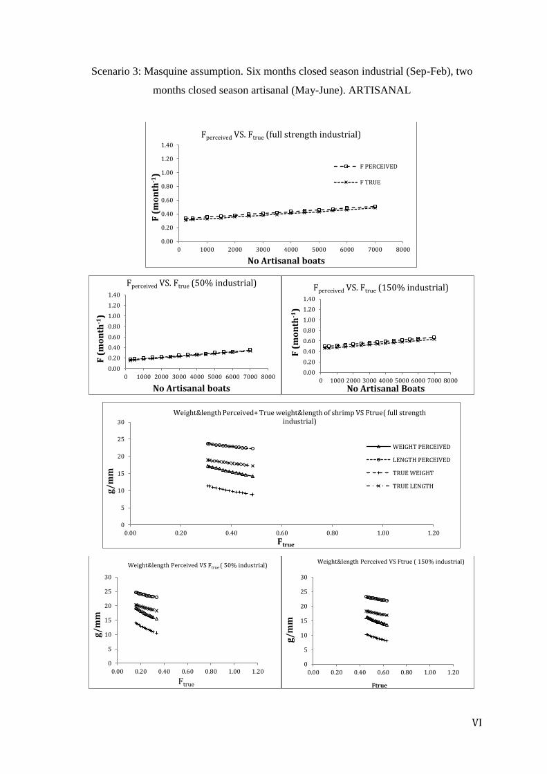
VI

Scenario 3: Masquine assumption. Six months closed season industrial (Sep-Feb), two

months closed season artisanal (May-June). ARTISANAL

0.00

0.20

0.40

0.60

0.80

1.00

1.20

1.40

0 1000 2000 3000 4000 5000 6000 7000 8000

F (

mo

nth

-1)

No Artisanal boats

Fperceived VS. Ftrue (full strength industrial)

F PERCEIVED

F TRUE

0.00

0.20

0.40

0.60

0.80

1.00

1.20

1.40

0 1000 2000 3000 4000 5000 6000 7000 8000

F (

mo

nth

-1)

No Artisanal boats

Fperceived VS. Ftrue (50% industrial)

0.00

0.20

0.40

0.60

0.80

1.00

1.20

1.40

0 1000 2000 3000 4000 5000 6000 7000 8000

F (

mo

nth

-1)

No Artisanal Boats

Fperceived VS. Ftrue (150% industrial)

0

5

10

15

20

25

30

0.00 0.20 0.40 0.60 0.80 1.00 1.20

g/

mm

Ftrue

Weight&length Perceived+ True weight&length of shrimp VS Ftrue( full strength industrial)

WEIGHT PERCEIVED

LENGTH PERCEIVED

TRUE WEIGHT

TRUE LENGTH

0

5

10

15

20

25

30

0.00 0.20 0.40 0.60 0.80 1.00 1.20

g/

mm

Ftrue

Weight&length Perceived VS Ftrue ( 50% industrial)

0

5

10

15

20

25

30

0.00 0.20 0.40 0.60 0.80 1.00 1.20

g/

mm

Ftrue

Weight&length Perceived VS Ftrue ( 150% industrial)

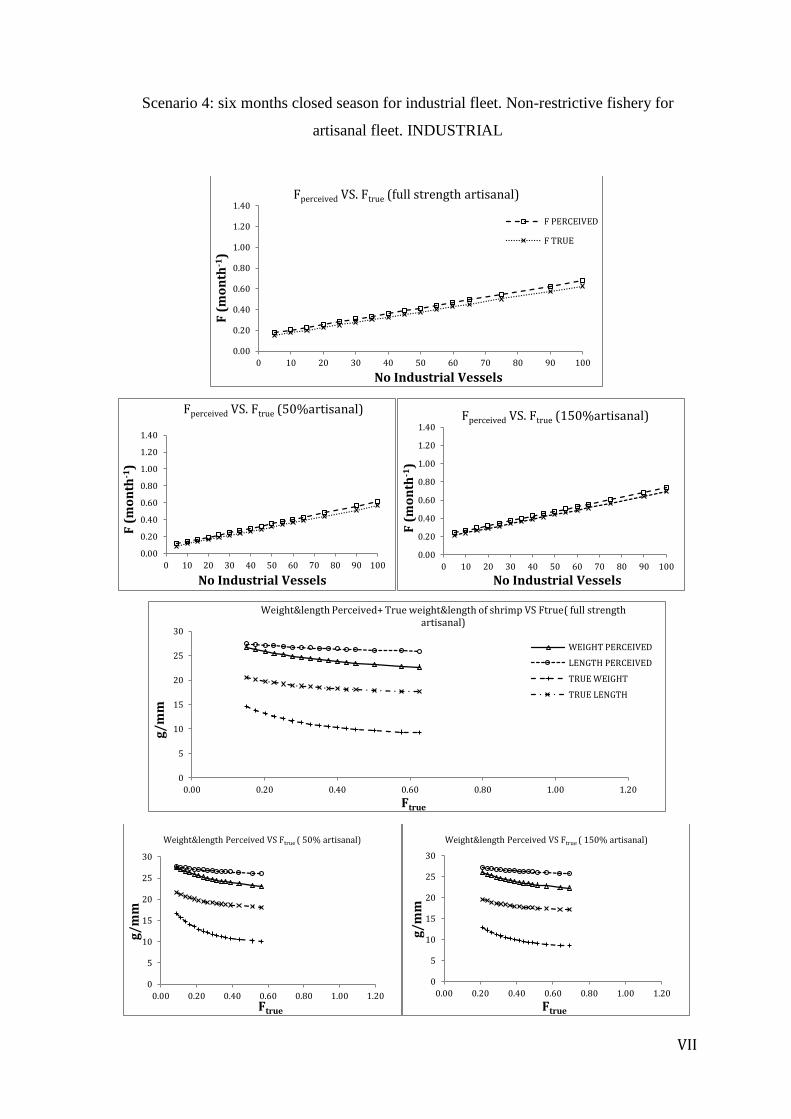
VII

Scenario 4: six months closed season for industrial fleet. Non-restrictive fishery for

artisanal fleet. INDUSTRIAL

0.00

0.20

0.40

0.60

0.80

1.00

1.20

1.40

0 10 20 30 40 50 60 70 80 90 100

F (

mo

nth

-1)

No Industrial Vessels

Fperceived VS. Ftrue (full strength artisanal)

F PERCEIVED

F TRUE

0.00

0.20

0.40

0.60

0.80

1.00

1.20

1.40

0 10 20 30 40 50 60 70 80 90 100

F (

mo

nth

-1)

No Industrial Vessels

Fperceived VS. Ftrue (50%artisanal)

0.00

0.20

0.40

0.60

0.80

1.00

1.20

1.40

0 10 20 30 40 50 60 70 80 90 100

F (

mo

nth

-1)

No Industrial Vessels

Fperceived VS. Ftrue (150%artisanal)

0

5

10

15

20

25

30

0.00 0.20 0.40 0.60 0.80 1.00 1.20

g/

mm

Ftrue

Weight&length Perceived+ True weight&length of shrimp VS Ftrue( full strength artisanal)

WEIGHT PERCEIVED

LENGTH PERCEIVED

TRUE WEIGHT

TRUE LENGTH

0

5

10

15

20

25

30

0.00 0.20 0.40 0.60 0.80 1.00 1.20

g/

mm

Ftrue

Weight&length Perceived VS Ftrue ( 50% artisanal)

0

5

10

15

20

25

30

0.00 0.20 0.40 0.60 0.80 1.00 1.20

g/

mm

Ftrue

Weight&length Perceived VS Ftrue ( 150% artisanal)

VIII

Scenario 4: six months closed season for industrial fleet. Non-restrictive fishery for

artisanal fleet. ARTISANAL

0.00

0.20

0.40

0.60

0.80

1.00

1.20

1.40

0 1000 2000 3000 4000 5000 6000 7000 8000

F (

mo

nth

-1)

No Artisanal Boats

Fperceived VS. Ftrue (full strength industrial)

F PERCEIVED

F TRUE

0.00

0.20

0.40

0.60

0.80

1.00

1.20

1.40

0 1000 2000 3000 4000 5000 6000 7000 8000

FF

(m

on

th-1

)

No Artisanal Boats

Fperceived VS. Ftrue (50% industrial)

0.00

0.20

0.40

0.60

0.80

1.00

1.20

1.40

0 1000 2000 3000 4000 5000 6000 7000 8000

F (

mo

nth

-1)

No Artisanal Boats

Fperceived VS. Ftrue (150% industrial)

0

5

10

15

20

25

30

0.00 0.20 0.40 0.60 0.80 1.00 1.20

g/

mm

Ftrue

Weight&length Perceived+ True weight&length of shrimp VS Ftrue( full strength industrial

WEIGHT PERCEIVED

LENGTH PERCEIVED

TRUE WEIGHT

TRUE LENGTH

0

5

10

15

20

25

30

0.00 0.20 0.40 0.60 0.80 1.00 1.20

g/

mm

Ftrue

Weight&length Perceived VS Ftrue ( 50% industrial)

0

5

10

15

20

25

30

0.00 0.20 0.40 0.60 0.80 1.00 1.20

g/

mm

Ftrue

Weight&length Perceived VS Ftrue ( 150% industrial)

IX

Scenario 5: Closed season of six months (Oct - Mar) for the industrial fleet, and one month

closure for the artisanal (Jan). INDUSTRIAL

0.00

0.20

0.40

0.60

0.80

1.00

1.20

1.40

0 10 20 30 40 50 60 70 80 90 100 110 120

F (

mo

nth

-1)

No Industrial Vessels

Fperceived VS. Ftrue (full strength artisanal)

F PERCEIVED

F TRUE

0.00

0.20

0.40

0.60

0.80

1.00

1.20

1.40

0 10 20 30 40 50 60 70 80 90 100

F (

mo

nth

-1)

No Industrial Vessels

Fperceived VS. Ftrue (50%artisanal)

0.00

0.20

0.40

0.60

0.80

1.00

1.20

1.40

0 10 20 30 40 50 60 70 80 90 100

F (

mo

nth

-1)

No Industrial Vessels

Fperceived VS. Ftrue (150%artisanal)

0

5

10

15

20

25

30

0.00 0.20 0.40 0.60 0.80 1.00 1.20

g/

mm

Ftrue

Weight&length Perceived+ True weight&length of shrimp VS Ftrue( full strength artisanal)

WEIGHT PERCEIVED

LENGTH PERCEIVED

TRUE WEIGHT

TRUE LENGTH

0

5

10

15

20

25

30

0.00 0.20 0.40 0.60 0.80 1.00 1.20

g/

mm

Ftrue

Weight&length Perceived VS Ftrue ( 50% artisanal)

0

5

10

15

20

25

30

0.00 0.20 0.40 0.60 0.80 1.00 1.20

g/

mm

Ftrue

Weight&length Perceived VS Ftrue ( 150% artisanal)

X

Scenario 5: Closed season of six months (Oct - Mar) for the industrial fleet, and one month

closure for the artisanal (Jan). ARTISANAL

0.00

0.20

0.40

0.60

0.80

1.00

1.20

1.40

0 1000 2000 3000 4000 5000 6000 7000 8000

F (

mo

nth

-1)

No Artisanal Boats

Fperceived VS. Ftrue (full strength industrial)

F PERCEIVED

F TRUE

0.00

0.20

0.40

0.60

0.80

1.00

1.20

1.40

0 1000 2000 3000 4000 5000 6000 7000 8000

F (

mo

nth

-1)

No Artisanal Boats

Fperceived VS. Ftrue (50% industrial)

0.00

0.20

0.40

0.60

0.80

1.00

1.20

1.40

0 1000 2000 3000 4000 5000 6000 7000 8000

F (

mo

nth

-1)

No Artisanal Boats

Fperceived VS. Ftrue (150% industrial)

0

5

10

15

20

25

30

0.00 0.20 0.40 0.60 0.80 1.00 1.20

g/

mm

Ftrue

Weight&length Perceived+ True weight&length of shrimp VS Ftrue( full strength industrial)

WEIGHT PERCEIVED

LENGTH PERCEIVED

TRUE WEIGHT

TRUE LENGTH

0

5

10

15

20

25

30

0.00 0.20 0.40 0.60 0.80 1.00 1.20

g/

mm

Ftrue

Weight&length Perceived VS Ftrue ( 50% industrial)

0

5

10

15

20

25

30

0.00 0.20 0.40 0.60 0.80 1.00 1.20

g/

mm

Ftrue

Weight&length Perceived VS Ftrue ( 150% industrial)

XI

Scenario 6: Closed season of six months (Oct - Mar) for the industrial fleet, and two months

closure for the artisanal (Jan-Feb). INDUSTRIAL

0.00

0.20

0.40

0.60

0.80

1.00

1.20

1.40

0 10 20 30 40 50 60 70 80 90 100

F (

mo

nth

-1)

No Industrial Vessels

Fperceived VS. Ftrue (full strength artisanal)

F PERCEIVED

F TRUE

0.00

0.20

0.40

0.60

0.80

1.00

1.20

1.40

0 10 20 30 40 50 60 70 80 90 100

F (

mo

nth

-1)

No Industrial Vessels

Fperceived VS. Ftrue (50%artisanal)

0.00

0.20

0.40

0.60

0.80

1.00

1.20

1.40

0 10 20 30 40 50 60 70 80 90 100

F (

mo

nth

-1)

No Industrial Vessels

Fperceived VS. Ftrue (150%artisanal)

0

5

10

15

20

25

30

0.00 0.20 0.40 0.60 0.80 1.00 1.20

g/

mm

Ftrue

Weight&length Perceived+ True weight&length of shrimp VS Ftrue( full strength artisanal)

WEIGHT PERCEIVED

LENGTH PERCEIVED

TRUE WEIGHT

TRUE LENGTH

0

5

10

15

20

25

30

0.00 0.20 0.40 0.60 0.80 1.00 1.20

g/

mm

Ftrue

Weight&length Perceived VS Ftrue ( 50% artisanal)

0

5

10

15

20

25

30

0.00 0.20 0.40 0.60 0.80 1.00 1.20

g/

mm

Ftrue

Weight&length Perceived VS Ftrue ( 150% artisanal)

XII

Scenario 6: Closed season of six months (Oct - Mar) for the industrial fleet, and two months

closure for the artisanal (Jan-Feb). ARTISANAL

0.00

0.20

0.40

0.60

0.80

1.00

1.20

1.40

0 1000 2000 3000 4000 5000 6000 7000 8000

F (

mo

nth

-1)

No Artisanal Boats

Fperceived VS. Ftrue (full strength industrial)

F PERCEIVED

F TRUE

0.00

0.20

0.40

0.60

0.80

1.00

1.20

1.40

0 1000 2000 3000 4000 5000 6000 7000 8000

FF (

mo

nth

-1)

No Artisanasl Boats

Fperceived VS. Ftrue (50% industrial)

0.00

0.20

0.40

0.60

0.80

1.00

1.20

1.40

0 1000 2000 3000 4000 5000 6000 7000 8000

F (

mo

nth

-1)

No Artisanal Boats

Fperceived VS. Ftrue (150% industrial)

0

5

10

15

20

25

30

0.00 0.20 0.40 0.60 0.80 1.00 1.20

g/

mm

Ftrue

Weight&length Perceived+ True weight&length of shrimp VS Ftrue( full strength industrial)

WEIGHT PERCEIVED

LENGTH PERCEIVED

TRUE WEIGHT

TRUE LENGTH

0

5

10

15

20

25

30

0.00 0.20 0.40 0.60 0.80 1.00 1.20

g/

mm

Ftrue

Weight&length Perceived VS Ftrue ( 50% industrial)

0

5

10

15

20

25

30

0.00 0.20 0.40 0.60 0.80 1.00 1.20

g/

mm

Ftrue

Weight&length Perceived VS Ftrue ( 150% industrial)

XIII

Table 1: 1st scenario values obtained at status quo of both fleets at different levels of background strengths.

YIELD( t) PROFIT($K) MEY

( vessels)

FTRUE

(month-1)

SHRIMP

LENGTH(mm)

SHAD

YIELD(t)

BY-CATCH

(t)

INDUSTRIAL

50% 7330 -12680 17 0.66 25.62 46700 6300

100% 5968 -20966 12 0.73 25.52 48150 3315

150% 4896 -27459 10 0.79 25.43 48100 2240

ARTISANAL

50% 2443 -1973 1000 0.43 23.72 51800 1700

100% 1515 -6687 1000 0.73 23.19 48150 3315

150% 1096 -10079 1000 1.03 22.90 45000 4800

Table 2: 2nd scenario values obtained at status quo of both fleets at different levels of background strengths.

YIELD( t) PROFIT($K) MEY

( vessels)

FTRUE

(month-1)

SHRIMP

LENGTH(mm)

SHAD

YIELD(t)

BY-CATCH

(t)

INDUSTRIAL

50% 7574 -10425 17 0.50 26.09 47800 6000

100% 6542 -16832 15 0.55 26.01 51500 3270

150% 5699 -22039 11 0.59 25.94 52100 2220

ARTISANAL

50% 2357 -93 1300 0.32 24.72 54200 1700

100% 1478 -3905 1200 0.55 24.24 51500 3270

150% 1067 -6687 1100 0.77 23.98 49000 4700

Table 3: 3rd scenario values obtained at status quo of both fleets at different levels of background strengths. YIELD( t) PROFIT($K) MEY

( vessels)

FTRUE

(month-1)

SHRIMP

LENGTH(mm)

SHAD

YIELD(t)

BY-CATCH

(t)

INDUSTRIAL

50% 6752 -15274 17 0.35 26.17 49700 4600

100% 5565 -22742 12 0.41 26.01 52300 2590

150% 4642 -28509 7 0.46 25.86 52400 1800

ARTISANAL

50% 2955 643 1000 0.26 23.54 54300 1350

100% 2267 -2250 1000 0.41 22.78 52300 2590

150% 1963 -4143 1000 0.56 22.39 50500 3700

XIV

Table 4: 4th scenario values obtained at status quo of both fleets at different levels of background strengths.

YIELD( t) PROFIT($K) MEY

( vessels)

FTRUE

(month-1)

SHRIMP

LENGTH(mm)

SHAD

YIELD(t)

BY-CATCH

(t)

INDUSTRIAL

50% 6390 -17110 15 0.36 26.46 51600 3050

100% 4955 -26169 10 0.43 26.28 52800 1350

150% 3903 -32767 6 0.49 26.11 53100 800

ARTISANAL

50% 3544 2257 1000 0.28 23.60 53600 700

100% 2806 -472 1000 0.43 22.98 52800 1350

150% 2469 -1975 1000 0.58 22.63 51800 2000

Table 5: 5th scenario values obtained at status quo of both fleets at different levels of background strengths.

YIELD( t) PROFIT($K) MEY

( vessels)

FTRUE

(month-1)

SHRIMP

LENGTH(mm)

SHAD

YIELD(t)

BY-CATCH

(t)

INDUSTRIAL

50% 6563 -15985 17 0.36 26.50 52000 3300

100% 5224 -24438 12 0.42 26.35 54000 1450

150% 4183 -30962 10 0.47 26.22 53600 900

ARTISANAL

50% 3381 2516 1000 0.27 23.91 55000 750

100% 2630 -311 1100 0.42 23.31 54000 1450

150% 2284 -1823 1000 0.57 22.96 52600 2100

Table 6: 6th scenario values obtained at status quo of both different fleets at different levels of background strengths.

YIELD( t) PROFIT($K) MEY

( vessels)

FTRUE

(month-1)

SHRIMP

LENGTH(mm)

SHAD

YIELD(t)

BY-CATCH

(t)

INDUSTRIAL

50% 6830 -14287 17 0.35 26.53 51300 3900

100% 5636 -21836 13 0.41 26.41 54400 1800

150% 4724 -27575 7 0.46 26.30 54300 1050

ARTISANAL

50% 3091 2490 1300 0.26 24.35 56100 900

100% 2300 -412 1100 0.41 23.74 54400 1800

150% 1941 -2272 1000 0.56 23.39 52500 2600