RF, Microwave & Wireless · 2018. 10. 4. · Physical causes of nonlinearity Operation under finite...
44
RF, Microwave & Wireless All rights reserved 1
Transcript of RF, Microwave & Wireless · 2018. 10. 4. · Physical causes of nonlinearity Operation under finite...

RF, Microwave & Wireless
All rights reserved1

All rights reserved 2
Non-Linearity Phenomenon

Physical causes of nonlinearity
►Operation under finite power-supply voltages
►Essential non-linear characteristics of electronic
active components (transistors, diodes, etc.)
►Mismatch of input signal levels to a design
►Mismatch of number of input signals to a design
All rights reserved 3

Problems caused by nonlinear distortions
►Transmission
Harmonics
Emission Mask spillover
EVM and Image Rejection degradation
Reduce efficiency (by backoff)
All rights reserved 4

Problems caused by nonlinear distortions
►Reception
Spurii (“signals” show up, even if
nonexistent at input)
Reduce dynamic range
Reduce sensitivity (desensitization)
Blocking of desired signals
All rights reserved 5
Harmonic Distortion
6
f 1 3f 1 4f 1 5f 12f 1
All rights reserved

Intermodulation
7
Fundamental
Distortion Products
(Spurii)
All rights reserved

Blocking (De-Sensing)
8
The presence of
an adjacent strong
signal blocks the
weak signal
All rights reserved

in in
out out Gain
Reduced
Gain
Small Signal
Linear Region
Saturation
Region
Compression
9All rights reserved
1 dB compression point
►Definition
All rights reserved 10
The 1 dB compression point specifies the output power of an amplifier at which the output signal lags behind the nominal output power by 1 dB.

Compression
►Definition of the 1 dB compression point at the amplifier input (Pin/1dB) and at the amplifier output (Pout/1dB)
All rights reserved 11

Compression
►Gain versus output power and definition of the 1 dB
compression
All rights reserved 12

Linear Region
All rights reserved 13

Saturation Region
All rights reserved 14

Models of nonlinear blocks and their characterization
All rights reserved 15
Pout[dBm]
Pin[dBm]Pout[dBm]
Pin[dBm]
Pin[dBm]
∆Φ[deg.]
Pin[dBm]
∆Φ[deg.]
Linear Block
Non-Linear Block
Saturation
Amplitude ResponsePhase Response
@f0
@f0
AM-AM AM-PM

Nonlinearities
►An ideal amplifier
All rights reserved 16
The connection to the input and output voltage is as follows:
The voltage transfer function of the linear two-port is as follows:

Nonlinearities
►In practice
All rights reserved 17
where vout(t) voltage at output of two-port
vin(t) voltage at input of two port
a0 DC component
a1 gain √G
an coefficients of the nonlinear
element of the voltage gain

Single-tone driving – Harmonics
► If a single sinusoidal signal vin(t) is applied to the input of the two port
All rights reserved 18
this is referred to as single-tone driving.

Single-tone driving – Harmonics
►Applying the trigonometric identity:
All rights reserved 19

Single-tone driving – Harmonics
►Spectrum before and after a nonlinear two-port block:
All rights reserved 20
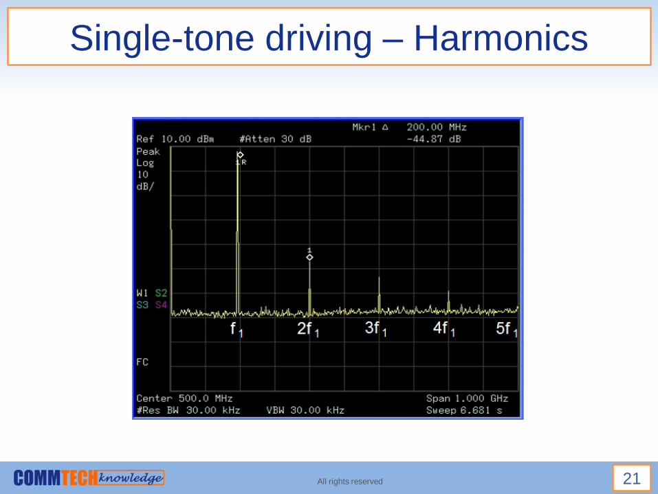
Single-tone driving – Harmonics
All rights reserved 21

Single-tone driving – Harmonics
► The levels of harmonics increase over
proportionally with their order as the input
level increases, i.e.
Changing the input level by A dB
Changes the nth harmonic level by n · A dB
All rights reserved 22
Note: This assumes the memory-less modelling applies.

Two-tone driving – Intermodulation
►Two-tone driving applies a signal v(t) into the input of
the two-port block.
►This signal consists of the sum of two sinusoidal
harmonic tones.
All rights reserved 23

Two-tone driving – Intermodulation
► The new frequencies produced may be evaluated using the
following trigonometric identities:
All rights reserved 24

Intermodulation products up to max. 3rd order with two-tone driving
All rights reserved 25
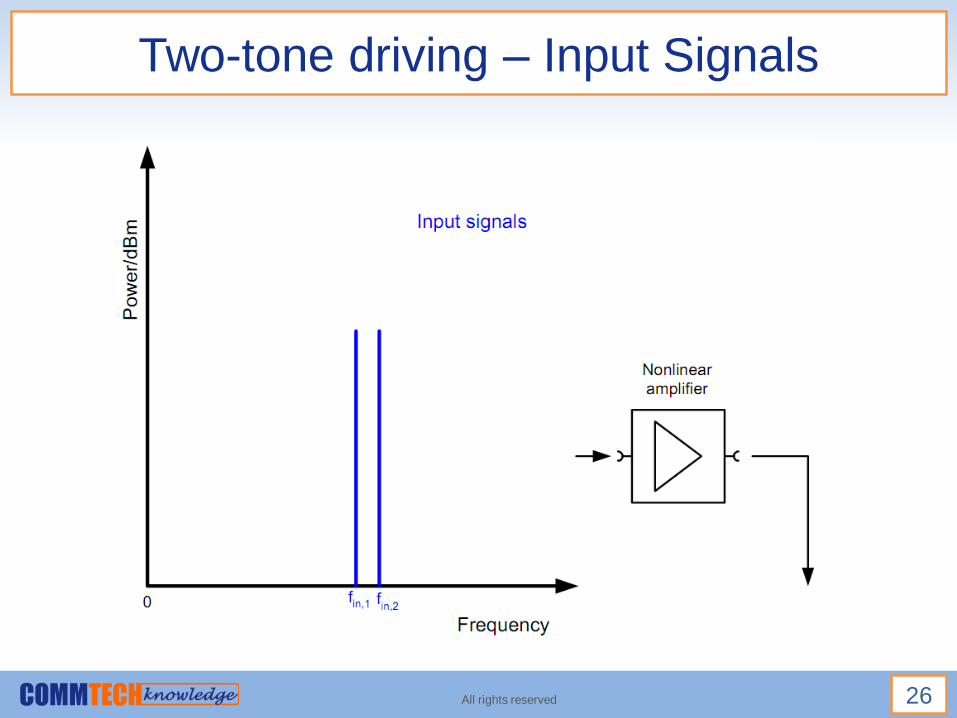
Two-tone driving – Input Signals
All rights reserved 26
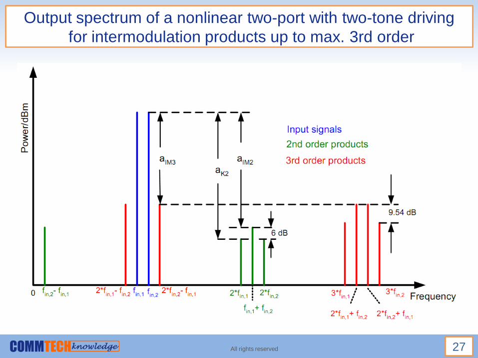
Output spectrum of a nonlinear two-port with two-tone driving
for intermodulation products up to max. 3rd order
All rights reserved 27

In-Band and Harmonic Band Spectra
All rights reserved 28
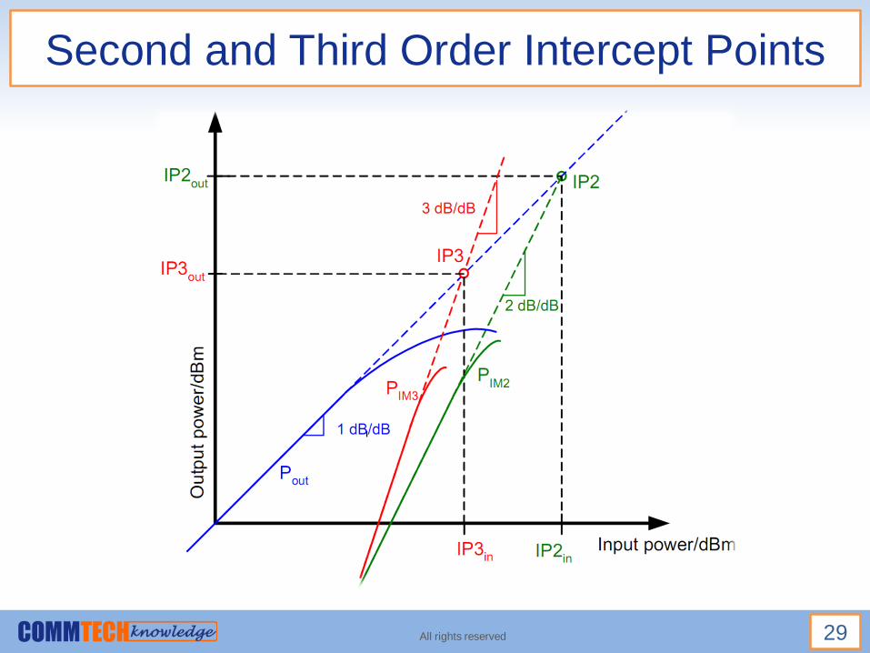
Second and Third Order Intercept Points
All rights reserved 29
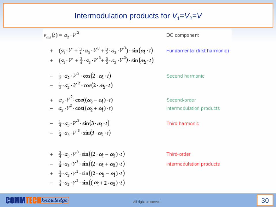
Intermodulation products for V1=V2=V
All rights reserved 30

Slope of OIP2 and OIP3 vs. Pin [dBm]
►The log-log power plot of IM2 is of slope 2dB/dB
►The log-log power plot of IM3 is of slope 3dB/dB
►The log-log power plot of IMN is of slope NdB/dB
All rights reserved 31

The third-order intercept and 1 dB compression points
All rights reserved 32
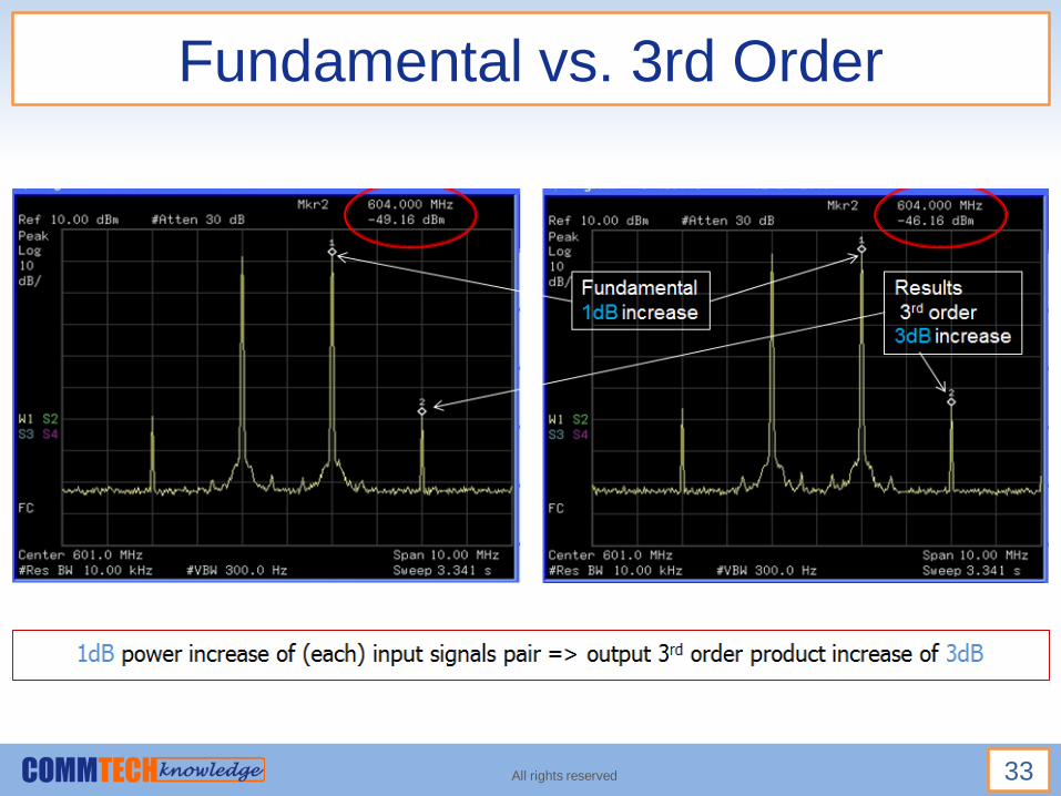
Fundamental vs. 3rd Order
All rights reserved 33

OIP3 and OIM3 – Linear Scale
All rights reserved 34
3
3
32 2 2
213 3
2
1
3IP
3
1out1 3IP
3
2
2 3 3
out3 3 in 3 in
2
6 3 3 331 in in3 2
1 3
a A 9 AAt IP : a
2 4 2
aA 2thus .
2 3 a
a2P OIP .
3 a
9 3Also IM a P a P
4 2
a3 1a P G P
2 a OIP
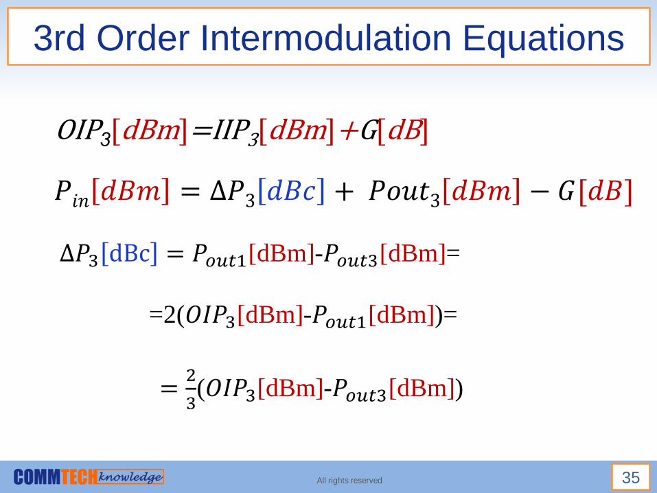
3rd Order Intermodulation Equations
All rights reserved 35
OIP3[dBm]=IIP3[dBm]+G[dB]
𝑃𝑖𝑛 𝑑𝐵𝑚 = ∆𝑃3 𝑑𝐵𝑐 + 𝑃𝑜𝑢𝑡3 𝑑𝐵𝑚 − 𝐺[𝑑𝐵]
∆𝑃3 dBc = 𝑃𝑜𝑢𝑡1[dBm]-𝑃𝑜𝑢𝑡3[dBm]=
=2(𝑂𝐼𝑃3[dBm]-𝑃𝑜𝑢𝑡1[dBm])=
=2
3(𝑂𝐼𝑃3[dBm]-𝑃𝑜𝑢𝑡3[dBm])

3rd Order Intermodulation Equations (2)
All rights reserved 36
𝑂𝐼𝑃3[dBm]=𝑃𝑜𝑢𝑡1[dBm]+ ∆𝑃3 dBc
2
𝑃𝑜𝑢𝑡3[dBm]= 3𝑃𝑖𝑛[dBm]+3G[dB]-2 𝑂𝐼𝑃3[dBm] =
= 3𝑃𝑜𝑢𝑡1[dBm]-2 𝑂𝐼𝑃3[dBm]

Spurious Free Dynamic Range
►Definition
Maximal to minimal input signal power ratio in dB
Maximal signal such that the 2-Tone IM products
are at the output noise power level
Minimal signal equals the sensitivity with a
prescribed SNRout.
Assume here SNRout=1 (0dB).
All rights reserved 37

Spurious Free Dynamic Range (cont’d)
All rights reserved 38
For 3rd order IM Products at the noise level:
If SNRout ≠ 0dB in the sensitivity definition, then:
3
2[ 10log( ( ) )]
3[ ]in r out
SDR OIP kT BF G
NdB
3
2[ 10log( [ ])]
3in rDR OIP kT BF G dB
∆𝑃3 dBc =2
3(𝑂𝐼𝑃3[dBm]-𝑃𝑜𝑢𝑡3[dBm])

Cascade Intercept Point
Assuming incoherent combining of IM products it
is possible to show that:
All rights reserved 39
2nd Order IM’s:
3rd Order IM’s:
(1) (2) ( 1) ( )
2 2 2 3 2 2 2
1 1 1 1 1...
sys N N
N N NOIP G G OIP G G OIP G OIP OIP
2 (1) 2 (2) 2 ( 1) 2 ( ) 2
3 2 3 3 3 3 3
1 1 1 1 1...
( ) ( ) ( ) ( ) ( )sys N N
N N NOIP G G OIP G G OIP G OIP OIP

Cascade Intercept Point – Another Form
Assuming incoherent combining of IM products it
is possible to show that:
All rights reserved 40
2nd Order IM’s:
3rd Order IM’s:
(1) (2) ( )
2 1 2 1 2 2 2
1...T T T
sys N
T
G G G
OIP G OIP G G OIP G OIP
2 2 2
2 (1) 2 (2) 2 ( ) 2
3 1 3 1 2 3 3
1...
( ) ( ) ( ) ( )
T T T
sys N
T
G G G
OIP G OIP G G OIP G OIP

Measuring Nonlinear Behavior
Most common measurements: Second level
using a network analyzer and power sweeps
gain compression
AM to PM conversion
using a spectrum analyzer + source(s)
harmonics, particularly second and third
intermodulation products resulting from two or more RF carriers
All rights reserved 41

Two Tone Test – Setup
All rights reserved 42

Third order Spurious Free Dynamic Range, SFRD-3
►Spurious Free Dynamic Range
►Definition
Maximal to minimal input signal power ratio in dB
Maximal signal such that the 2-Tone IM products are at the output noise power level
Minimal signal equals the sensitivity with a prescribed SNRout. Assume here (or if not specified otherwise) SNRout=1 (0dB).
All rights reserved 43

Design Tradeoffs between linearity and Sensitivity Optimization
►Sensitivity Optimization
First stage with high gain
First stage with low NF
►Linearity Optimization
Limit the gain of the first stages
Last stage with high IP
All rights reserved 44

![Nonlinearity of Microwave Electric Field Coupled Rydberg ...laserspec.sxu.edu.cn/docs/2019-06/1a7dcc2a347349fdaaddfae335d… · external electric fields [9–15]. Rydberg electromagnetically](https://static.fdocuments.in/doc/165x107/5f08c7447e708231d423ada1/nonlinearity-of-microwave-electric-field-coupled-rydberg-external-electric-ields.jpg)