ISSN 0120-9957 July-September 2019 Revista Colombiana de ...

Revista
Colombiana
de EstadısticaNumero especial en Bioestadıstica
Volumen 35. Numero 2 - junio - 2012 ISSN 0120 - 1751
UNIVERSIDAD
NACIONALDE COLOMBIAS E D E B O G O T Á
FACULTAD DE CIENCIASDEPARTAMENTO DE ESTADÍSTICA

Revista Colombiana de Estadısticahttp://www.estadistica.unal.edu.co/revista
http://es.wikipedia.org/wiki/Revista Colombiana de Estadistica
http://www.emis.de/journals/RCE/
revcoles [email protected]
Indexada en: Ulrichsweb, Scopus, Science Citation Index Expanded (SCIE), Web of
Science (WoS), SciELO Colombia, Current Index to Statistics, Mathematical Reviews
(MathSci), Zentralblatt Fur Mathematik, Redalyc, Latindex, Publindex (A1)
Editor
Leonardo Trujillo, Ph.D.Universidad Nacional de Colombia, Bogota, Colombia
Editores invitados
Liliana Lopez-Kleine, Ph.D.Universidad Nacional de Colombia, Bogota, Colombia
B. Piedad Urdinola, Ph.D.Universidad Nacional de Colombia, Bogota, Colombia
Comite invitado
Thibaut Jombart, Ph.D.Imperial College, London
Susana Eyheramendy, Ph.D.Pontificia Universidad Catolica de Chile, Chile
Alain Trubuil, Ph.D.Institut national de la Recherche Agronomique, France
Raul Machiavelli, Ph.D.University of Puerto Rico at Mayaguez, Puerto Rico
Dirk Husmeier, Ph.D.Biomathematics and Statistics Scotland (BioSS), United Kingdom
Stephane Robin, Ph.D.Agro Paris Tech, France
Bernardo Lanza Queiroz, Ph.D.Universidade Federal de Minas Gerais, Brazil
Bernardo Antonio Sanhueza, Ph.D.Universidad de La Frontera, Chile
La Revista Colombiana de Estadıstica es una publicacion semestral del Departamento deEstadıstica de la Universidad Nacional de Colombia, sede Bogota, orientada a difundir conoci-mientos, resultados, aplicaciones e historia de la estadıstica. La Revista contempla tambien lapublicacion de trabajos sobre la ensenanza de la estadıstica.
Se invita a los editores de publicaciones periodicas similares a establecer convenios de canjeo intercambio.
Direccion Postal:Revista Colombiana de Estadısticac© Universidad Nacional de Colombia
Facultad de CienciasDepartamento de EstadısticaCarrera 30 No. 45-03Bogota – ColombiaTel: 57-1-3165000 ext. 13231Fax: 57-1-3165327
Adquisiciones:Punto de venta, Facultad de Ciencias, Bogota.Suscripciones:revcoles [email protected] de artıculos:Se pueden solicitar al Editor por correo fısico oelectronico; los mas recientes se pueden obteneren formato PDF desde la pagina Web.
Edicion en LATEX: Patricia Chavez R. E-mail: [email protected]
Impresion: Editorial Universidad Nacional de Colombia, Tel. 57-1-3165000 Ext. 19645, Bogota.

Revista Colombiana de Estadıstica Bogota Vol. 35 No 2
ISSN 0120 - 1751 COLOMBIA junio-2012 Pags. 185-330
Numero especial en Bioestadıstica
Contenido
Francisco J. Torres-Aviles, Gloria Icaza & Reinaldo B.Arellano-ValleAn Extension to the Scale Mixture of Normals for Bayesian Small-Area
Estimation . . . . . . . . . . . . . . . . . . . . . . . . . . . . . . . . . . . . . . . . . . . . . . . . . . . . . . . . . . . . . . . . . . . . 185-204
Monica Catalan, M. Purificacion Galindo, Javier Martın& Vıctor LeivaMetodos de integracion de odds ratio basados en meta-analisis usando
modelos de efectos fijos y aleatorios utiles en salud publica . . . . . . . . . . . . . . . . . . . . . 205-222
Diego Alejandro Salazar, Jorge Ivan Velez & Juan Carlos SalazarComparison between SVM and Logistic Regression: Which One is Better
to Discriminate? . . . . . . . . . . . . . . . . . . . . . . . . . . . . . . . . . . . . . . . . . . . . . . . . . . . . . . . . . . . . . . 223-237
Carlos Mario Lopera-Gomez, Mario Cesar Jaramillo-Elorza& Natalia Acosta-Baena¿Cuando inicia la enfermedad de Alzheimer? Kaplan-Meier versus Turnbull:
una aplicacion a datos con censura arbitraria . . . . . . . . . . . . . . . . . . . . . . . . . . . . . . . . . . 239-254
Eduardo Davila, Luis Alberto Lopez & Luis Guillermo DıazA Statistical Model for Analyzing Interdependent Complex of Plant Pathogens . . 255-270
Minerva Montero, Maria Elena Dıaz, Santa Jimenez, Iraida Wong& Vilma MorenoModelacion de indicadores del estado nutricional de la embarazada desde
un enfoque multinivel . . . . . . . . . . . . . . . . . . . . . . . . . . . . . . . . . . . . . . . . . . . . . . . . . . . . . . . . . . 271-287
Rajvir Singh, Vrijesh Tripathi, Mani Kalaivani, Kalpana Singh& S.N. DwivediDeterminants of Birth Intervals in Tamil Nadu in India: Developing Cox
Hazard Models with Validations and Predictions . . . . . . . . . . . . . . . . . . . . . . . . . . . . . . . 289-307
Carlos Alberto Martınez, Mauricio Elzo, Carlos Manrique,Luis Fernando Grajales & Ariel JimenezRandom Regression Models for Estimation of Covariance Functions, Genetic
Parameters and Prediction of Breeding Values for Rib Eye Area in
a Colombian Bos indicus-Bos taurus Multibreed Cattle Population . . . . . . . . . . . . . .309-330


Editorial
Número especial de la Revista Colombiana de Estadística en
Bioestadística
Liliana López-Kleinea, B. Piedad Urdinolab
Departamento de Estadística, Facultad de Ciencias, Universidad Nacional de
Colombia, Bogotá, Colombia
La importancia de la bioestadística es innegable. Sus aplicaciones cubren áreas
aparentemente disímiles, como medicina, zoología, demografía, genética, agricul-
tura, epidemiología, veterinaria y biología con un común, el cual son los desarrollos
en la estadística que ayudan a resolver problemas teóricos, aplicados y más recien-
temente computacionales.
Colombia, con todo su potencial en biodiversidad, agrícola, sus recursos huma-
nos y el despegue reciente de la investigación no puede ser el gran ausente en los
aportes que cada vez son más y mejores en esta área de la estadística. Con este
objetivo en mente decidimos convocar este número especial en Bioestadística para
la Revista Colombiana de Estadística.
Con éxito recibimos 18 trabajos que cubrieron todos los sub-temas dentro de la
bioestadística. Nueve de ellos, que en efecto cubren preguntas de gran relevancia
teórica, aplicaciones en epidemiología, demografía, estudios genómicos y biológi-
cos, y en salud pública fueron seleccionados para publicación luego del proceso
arbitral. Esperamos que estos trabajos sean una motivación para muchos investi-
gadores y grupos de investigación multidisciplinarios para el desarrollo de teorías
en bioestadística y aplicaciones en diversas áreas de las ciencias biológicas. Igual-
mente, esperamos que sean de gran utilidad para el caso colombiano que cada día
cuenta con mayores y mejores datos en todas estas áreas y para la bioestadística
en general.
Agradecemos en particular la participación y apoyo de los miembros del Comité
Invitado, cuyo dedicado trabajo y el de los árbitros permitieron que esta empresa
fuera posible y a la Asistenta Editorial de la revista. Gracias,
aEditora invitada del número especial de la Revista Colombiana de Estadística.
Profesora asociada. E-mail: [email protected] invitada del número especial de la Revista Colombiana de Estadística.
Profesora asociada. E-mail: [email protected]


Revista Colombiana de EstadísticaNúmero especial en Bioestadística
Junio 2012, volumen 35, no. 2, pp. 185 a 204
An Extension to the Scale Mixture of Normals forBayesian Small-Area Estimation
Una extensión a la mezcla de escala de normales para la estimaciónBayesiana en pequeñas áreas
Francisco J. Torres-Avilés1,a, Gloria Icaza2,b,Reinaldo B. Arellano-Valle3,c
1Departamento de Matemática y Ciencia de la Computación, Facultad de Ciencia,Universidad de Santiago de Chile, Santiago, Chile
2Instituto de Matemática y Física, Universidad de Talca, Talca, Chile3Departamento de Estadística, Facultad de Matemáticas, Pontificia Universidad
Católica de Chile, Santiago, Chile
Abstract
This work considers distributions obtained as scale mixture of normaldensities for correlated random variables, in the context of the Markov ran-dom field theory, which is applied in Bayesian spatial intrinsically autoregres-sive random effect models. Conditions are established in order to guaranteethe posterior distribution existence when the random field is assumed asscale mixture of normal densities. Lung, trachea and bronchi cancer rela-tive risks and childhood diabetes incidence in Chilean municipal districts areestimated to illustrate the proposed methods. Results are presented usingappropriate thematic maps. Inference over unknown parameters is discussedand some extensions are proposed.
Key words: Disease mapping, Markov random field, Hierarchical model,Incidence rate, Relative risk.
Resumen
Este trabajo aborda las distribuciones obtenidas como mezcla de escala denormales para variables aleatorias correlacionadas, en el contexto de la teoríade los campos markovianos, la cual es aplicada a modelos bayesianos espa-ciales con efectos aleatorios autoregresivos intrínsecos. Se establecen condi-ciones para garantizar la existencia de la distribución a posteriori cuando se
aAssistant professor. E-mail: [email protected] professor. E-mail: [email protected]. E-mail: [email protected]
185

186 Francisco J. Torres-Avilés, Gloria Icaza & Reinaldo B. Arellano-Valle
asume una distribución mezcla de escala de normales para el campo marko-viano propuesto. Para ilustrar los métodos propuestos, se estiman los riesgosrelativos de cáncer de tráquea, bronquios y pulmón, y tasas de incidencia dediabetes tipo 1 en distritos municipales de Chile. Los resultados son presen-tados usando mapas temáticos apropiados. Se discute la inferencia sobre losparámetros desconocidos y se proponen algunas extensiones.
Palabras clave: campo aleatorio markoviano, mapeo de enfermedades, mod-elo jerárquico, riesgo relativo, tasa de incidencia.
1. Introduction
Over the last two decades, Bayesian spatial models have become increasinglypopular for epidemiologists and statisticians. In particular, small-area modeling isoriented to illustrate the behavior of rates or relative risks associated to each dis-trict that form a region or a country, that is, recognition of spatial patterns throughmaps is the main aim of these methodologies. The conventional assumption to es-timate the standardized mortality ratios (SMRs) or incidence rates is based onthe Poisson distribution. This assumption may cause several problems in thisclass of studies, mainly because of the extra-poisson variation. This extra-Poissonvariation generally arises when the observed number of cases on each small-areaare more variable than the variation contributed by the standard Poisson model(Mollié 2000). Bayesian models have been developed to solve this problem, intro-ducing random effects to account for unobserved spatial heterogeneity; even more,Markov chain Monte Carlo (MCMC) methods led to an explosive increment of theuse of Bayesian analysis in these areas of application.
Important works that develop and use Bayesian theory are mentioned in thefollowing lines. The pioneering work in this direction was done by Clayton &Kaldor (1987) who proposed an empirical Bayes approach with application to lipcancer data in Scotland. In Ghosh, Natarajan, Stroud & Carlin (1998), conditionsto demonstrate Bayesian generalized linear model (GLM) integrability are formal-ized under improper prior assumptions in order to represent lack of knowledge overunknown parameters. Best, Arnold, Thomas, Waller & Collon (1999) investigatedseveral spatial prior distributions based on Markov random field (MRF) theory,and discussed methods for model comparison and diagnostics. Pascutto, Wake-field, Best, Richardson, Bernardinelli, Staines & Elliott (2000) examined somestructural and functional assumptions of these models and illustrated their sensi-tivity through the presentation of results related to informal sensitivity analysisfor prior distributions choices. They also explored the effect caused by outlyingareas, assuming a Student-t distribution for the nonstructured effect.
Recently, Parent & Lesage (2008) proposed a linear Bayesian hierarchical modelto study the knowledge spillovers in European countries, under different specifica-tions of the proximity structures. They also compared this effect through differentstrategies, for example allowing different prior distributions or Student-t errors, toinclude heterogeneity in the disturbances.
Revista Colombiana de Estadística 35 (2012) 185–204

An Extension to the SMN 187
As it was previously mentioned, the class of spatial models has been related toGLM theory, considering random effects to represent the influence of geography.Besag (1974) presented a pioneering work in the context of the MRF theory, withapplications to regular lattice systems when spatial heterogeneity is considered.
Furthermore, the most used structure follows the work developed by Besag(1986), who presents a definition in the context of a MRF: Let u = (u1, u2, . . . , um)′
be a set of m random variables and u−i the random vector without the i-thcomponent, where m represents a number of different and contiguous areas. Ifthe joint distribution of u can be expressed by each conditional distribution, ui |u−i, i = 1, . . . ,m, then it is called a MRF. Intrinsically conditional autoregressive(CAR) random effects are defined as a particular MRF, initially proposed byBesag, York & Mollié (1991), which name is related to the impropriety of the jointdistribution generated by the univariate conditional distributions of ui | u−i, i =1, . . . ,m (see details in Banerjee, Carlin & Gelfand 2004).
In this work, an intrinsically Gaussian MRF is considered and its properties areextended to a more general family of continuous distributions. Scale mixture ofnormal (SMN) distributions have been proposed as robust extensions of the normalmodel. The genesis of this class of models is presented by Andrews & Mallows(1974). The SMN class of distributions is generated if the vector of interest, u,can be represented as
u = µ+ ψ−1/2z (1)
where µ is a location vector parameter, and z and ψ are independent, with zfollowing a multivariate zero centered normal distribution with covariance matrixΣ and ψ being a non-negative random scale factor with c.d.f. Fψ(· | ν), so thatFψ(0 | ν) = 0. Here ν is an additional or set of parameters controlling the kurtosisof the distribution of ψ. The SMN distributions have been shown to be a subclassof the elliptical distributions family by Fang, Kotz & Ng (1990). This subfamilypresents properties similar to the normal distributions, except that their behaviorallows capturing unusual patterns present in the data. In a Bayesian context,robust linear models have been studied since Zellner (1976). The multivariateStudent-t and the multivariate Slash distributions are examples of this class ofdistributions.
Following the above ideas, heavier-tailed models will be assumed instead ofworking with the usual assumption of normality for u, through the Student-tand Slash distributions developed by Geweke (1993) and Lange & Sinsheimer(1993), respectively. Specifically, the Slash distribution considered in this workcorresponds to the distribution of the random vector ψ−1/2z, where z and ψ areindependent, with z having a multivariate normal distribution as in (1) and ψ | νfollowing a distributionBeta(ν/2, 1), ν > 0. The Student-t distribution is obtainedthrough the same representation as the Slash distribution, with the difference thatψ | ν follows a Gamma distribution, where both parameters are equal to ν/2, ν > 0.There are some potential problems with the Slash distribution that probably hasresulted in more use of the Student-t. However, the Slash distribution may allowfor fatter tails (more extreme values) than the Student-t.
Revista Colombiana de Estadística 35 (2012) 185–204

188 Francisco J. Torres-Avilés, Gloria Icaza & Reinaldo B. Arellano-Valle
From a MRF context, the class of SMN can be found in papers developed from ageological point of view, where prediction is the main focus. Student-t distributedMRF was treated by Roislien & Omre (2006) using a frequentist approach. Lyu& Simoncelli (2007) made the extension of Gaussian MRF theory to what theycalled Gaussian scale mixture fields, for image reconstruction modeling.
In this work, Bayesian non-Gaussian spatial models are developed to detectunusual rates or relative risks in a particular area under the following scheme.Standard small-area models are presented in Section 2. SMN theory is appliedto extend the Gaussian MRF model (Besag 1974) in Section 3. In Section 4,non-Gaussian models are developed trough extensions of the spatial random effectfollowing a Gaussian MRF to the scale mixture of Normal random field (SMNRF) proposed previously. Three different models are used to estimate the incidencerates of Insulin Dependent Diabetes Mellitus (IDDM) in the Chilean MetropolitanRegion, and Respiratory Cancer mortality in the northern regions of Chile. Theseresults are presented in Section 5. Finally, some comments and discussion aremade in Section 6.
2. Spatial Models with Random Effects
Let y = (y1, . . . , ym)′ be a set of m random variables indexed to a specificregion. A general formulation is assumed from the generalized linear mixed modeltheory (Breslow & Clayton 1993), which includes the following elements:
1. A specification of the likelihood function as member of the exponential fam-ily, namely
f(y | θ,φ) =
m∏i=1
expφ−1i (yiθi − g(θi)) + ρ(φi; yi) (2)
where θ = (θ1, . . . , θm)′ is the vector of canonical parameters, φ = (φ1, . . . ,φm)′ is a vector of known scale parameters, g is a known function that doesnot depend on the data, and ρ is a known function that does not depend onthe unknown parameters.
2. A random specification for the link function, h(θi) = E(yi | θi), is typicallyrepresented by the normal linear mixed model
h(θi) | xi,β, ui, σ2 ind.∼ Normal(x′iβ + ui, σ2) (3)
where the xis are a p× 1 vectors of covariates associated to a p× 1 vector ofcoefficients β, the uis represent spatial random effects, and σ2 measures thenonstructured variability.
3. A model specification for the spatially structured random effects uis. Typ-ically, Gaussian assumptions for the uis are made. In the literature it isrecurrent to find that these spatial random effects are influenced by a prede-fined neighborhood represented by an adjacency matrix Dw, controlling the
Revista Colombiana de Estadística 35 (2012) 185–204

An Extension to the SMN 189
local variability. Hence, the mean is smoothed by the information given byits neighbors.
Let π(u | σ2u,Dw) = π(u1, . . . , um | σ2
u,Dw) be the joint probabilitydistribution derived from a MRF given a dispersion parameter σ2
u and am ×m m ×m adjacency matrix Dw. A multivariate Gaussian distributionis then obtained when,
π(u | σ2u,Dw) ∝ 1
(σ2u)m/2
exp
− 1
2σ2u
u′Dwu
(4)
A specific case is considered in this work, where Dw has diagonal ele-ments wi+ representing the number of neighbors of the i-th component, andoff-diagonal elements wij taking values −1 if the elements i and j shareboundary, denoted by i ∼ j, and 0 in other case, i.e.,
wij =
wi+ i = j
−1 i 6= j; i ∼ j0 otherwise.
(5)
Under 5, equation 4 is reduced to
π(u | σ2u,Dw) ∝ 1
(σ2u)m/2
exp
− 1
2σ2u
∑i∼j
(ui − uj)2 (6)
A basic discussion and treatment of several proximity matrices can be foundin Banerjee et al. (2004). A constraint will be imposed to this expression toguarantee integrability.
4. As a final step of the modeling, prior distributions are required for the un-known parameters to complete the hierarchical model. Usual non-informativeprior distributions are represented by
i. π(β) ∝ constantii. σ−2 ∼ Gamma(a/2, b/2)
iii. σ−2u ∼ Gamma(c/2, d/2)
(7)
where the improper prior π(β), β = (β1, β2, . . . , βp)′ ∈ Rp, is assumed ac-
cording with Ghosh et al. (1998). The hyperparameters a, b, c, d > 0 areknown constant. Here, both σ2 and σ2
u represent the dispersion parame-ters included in the model; σ2
u is the local dispersion parameter related toa specific spatial structure. Another useful measure in spatial models is thepercentage of spatial aggregation explained by the model, which usually ismeasured by the ratio
σ2u
σ2u + σ2
× 100% (8)
Its interpretation is related to obtain the relative contribution given by thespatial aggregation effect. Here, a common estimation of σ2
u is the empiricalvariance s2u, which can be obtained from the estimation of u for each MCMCiteration.
Revista Colombiana de Estadística 35 (2012) 185–204

190 Francisco J. Torres-Avilés, Gloria Icaza & Reinaldo B. Arellano-Valle
3. Scale mixture of Intrinsically CAR Models
In this section an extension of the usual multivariate Gaussian MRF is pro-posed, assuming a multivariate SMN distribution. The next definition will providean extension of (4) to the SMN random field (SMN RF).
Definition 1. A spatial random vector u = (u1, . . . , um)′ follows an SMN RF, ifthe kernel distribution can be obtained as
π(u | σ2u,Dw, ν) ∝
∫ ∞0
(ψ
σ2u
)m/2exp
− ψ
2σ2u
u′Dwu
dF (ψ | ν) (9)
where F (· | ν) is the c.d.f. of ψ | ν, σ2u is a dispersion parameter, and Dw denotes
a adjacency matrix. A SMN RF with scale parameter σ2u will be denoted as
SMNRF (0, σ−2u Dw, ν).
For the Gaussian case, it is known that specification of Dw in (5) makes (4)improper (Banerjee et al. 2004), since the matrix Dw is singular, so that its inversedoes not exist, hence∫
Rm
π(u | σ2u,Dw, ν)du ∝
∫Rm
1
(σ2u)m/2
exp
− 1
2σ2u
u′Dwu
du =∞
The last equation implies that a density function is available, but not inte-grable. This result is the intrinsic autoregressive model property, and it is usuallyrelegated to the prior distribution elicitation. If additional assumptions are notconsidered, the improper condition will imply that if a multivariate SMN RF isassumed with kernel (9), then consistent property (Kano 1994) fails. Therefore,integration theory can not be applied.
In the same way as the joint distribution of the Gaussian MRF treated in thespatial literature, for every SMN RF, the joint distribution will also be improper.In fact, this distribution will be proper only if the associated dispersion matrix isdefinite positive. Hence, some additional restrictions should be imposed to obtaina proper joint distribution, as discussed in Banerjee et al. (2004) and Assunção,Potter & Cavenaghi (2002). The next proposition establishes conditions to makeproper the associated SMN RF. The proof of this proposition can be found in theappendix.
Proposition 1. Suppose that a set of spatial indexed random variables, repre-sented by the vector u = (u1, . . . , um)′, is available. Consider the SMN RF in(9) as the distribution of u. Additionally, let us suppose that F (· | ν) is a knownpositive c.d.f. If
∑mi=1 ui = 0 and E(ψ1/2 | ν) <∞, then (9) is proper.
Specific choices for F (· | ν) in (9) lead to different scale mixture probabilitydistributions. Student-t and Slash MRFs will be used in this work, which canbe obtained using stochastic representations which depend on the selected mixingdistribution F (· | ν).
The SMN RF can be represented hierarchically in terms of two stages:
Revista Colombiana de Estadística 35 (2012) 185–204

An Extension to the SMN 191
At the first stage of the hierarchy, a Gaussian MRF is specified with an addi-tional random scale factor ψ. At the second stage, a mixing distribution for thescale perturbation ψ is then specified. Specifically:
1. For the Student-t MRF:
i) u | σ2u, ψ,Dw ∼ Normal
(0, σ−2u ψDw
)(10)
ii) ψ | ν ∼ Gamma(ν/2, ν/2) (11)
In this case, the Student-t MRF with ν degrees of freedom follows, which isdenoted by u | Dw, σ
2u, ν ∼ t(0, σ−2u Dw, ν).
2. For the Slash MRF:
i) u | σ2u, ψ,Dw ∼ Normal
(0, σ−2u ψDw
)(12)
ii) ψ | ν ∼ Beta(ν/2, 1) (13)
In this case, the Slash MRF, denoted by u | Dw, σ2u, ν ∼ Slash(0, σ−2u Dw, ν),
is obtained.
The model described above is useful to implement the MCMC method. It isimportant to mention that the distribution of both of the above random fields hasthe finite condition exposed in Proposition 1.
A prior distribution for ν is required in order to assume a valid Bayesian model.Usually, an exponential distribution prior is considered for this parameter, whichis assumed independent of (6), that is,
ν | δ0 ∼ exp(δ0), δ0 > 0 (14)
Assuming (2), (3), (7), (9) and (14), the full joint posterior distribution isspecified as,
π(θ,β,u, σ2u, σ
2, ψ, ν | y,Dw, δ0) ∝m∏i=1
expφ−1i (yiθi − g(θi))
×m∏i=1
exp−(1/2σ2)(h(θi)− x′iβ − ui)2h′(θi)
× exp−(ψ/2σ2u)u′Dwuψm/2(σ2σ2
u)−m/2
× exp−a/2σ2u(σ2)−(b/2+1)
exp−c/2σ2(σ2u)−(d/2+1)
× f(ψ | ν) exp−δ0ν
(15)
where fψ(· | ν) represents the conditional density or probability function of ψ | ν.See item 3 of the appendix for the computational aspects.
Revista Colombiana de Estadística 35 (2012) 185–204

192 Francisco J. Torres-Avilés, Gloria Icaza & Reinaldo B. Arellano-Valle
4. Proposed Bayesian Small-Area Models
An important point is to demonstrate the integrability of the proposed model.Under the generalized linear model (2), link function (3) and prior assumptiongiven by (7) and (14), Theorem 2 from the work developed by Ghosh et al. (1998)gives the conditions to obtain a proper posterior distribution for θ | y when P (ψ =1 | ν) = 1 (the Gaussian MRF). Following that theorem, it is possible to find ageneralization towards the SMN case.
The next proposition gives conditions when the spatial random effect followsan SMN RF. Its proof is given in the appendix.
Proposition 2. Consider the model (2), link function (3) and prior assumptiongiven by (7) and (14). Consider also the assumptions of Proposition 1 and thefollowing additional conditions:i. θi ∈ (θi, θi), for some −∞ < θi < θi <∞, i = 1, . . . ,m;ii. m− p+ a− 1 > 0;iii. b > 0, d > 0, m+ c > 0
If the condition of integrability∫ θi
θi
expφ−1i (yiθi − g(θi))h′(θi)dθi <∞
is verified for all i = 1, . . . ,m, then posterior distribution π(θ |y) is proper.
The main interest is focused in establishing a non-Gaussian parametric spatialrandom effect. A MCMC structure seems to be adequate to make inferences fromthis class of model. Most full conditional distributions computed for this schemeare known distributions, therefore, a hybrid Gibbs sampling - metropolis Hastingsalgorithm is used to generate samples from the joint posterior distribution. Thealgorithm given in item 3 of the appendix presents the full conditional distributionsfor this particular model.
5. Applications
The proposed spatial Bayesian models will be applied assuming SMN randomeffects for two real data in the epidemiological framework to control for exces-sive smoothness in small areas with sparse data. One dataset is related to IDDMincidence rates in the Chilean municipal districts from Metropolitan region andthe other dataset contains female lung, trachea and bronchi cancer standardizedmortality ratios in the municipal districts of the country’s northern zone. Themunicipal district is the smallest administrative area in Chile. In this countrythere are only few published studies related to spatial epidemiology (Andia, Hs-ing, Andreotti & Ferreccio 2008, Ferreccio, Rollán, Harris, Serrano, Gederlini,Margozzini, Gonzalez, Aguilera, Venegas & Jara 2007, Icaza, Núñez, Torres, Díaz& Varela 2007, Icaza, Núñez, Díaz & Varela 2006, Torres-Avilés, Icaza, Carrasco &
Revista Colombiana de Estadística 35 (2012) 185–204

An Extension to the SMN 193
Pérez-Bravo 2010). Results from non-Gaussian spatial Bayesian modeling relatedto both diseases are presented in the next subsections.
The specific model that is considered for these two applications is the Poissonhierarchical model given by
yi | ei, λiind.∼ Poisson(eiλi)
log(λi) | β0, ui, σ2 ind.∼ Normal(β0 + ui, σ2)
i = 1, . . . ,m, where y = (y1, . . . , ym)′ represents the observed sample vector asso-ciated to m different regions under study, e = (e1, . . . , em)′ represents the popula-tion at risk or the expected population associated to the m different regions, andu = (u1, . . . , um)′ is the vector of random effects which is assumed to have a SMNdistribution constrained to sum zero. Diffuse prior distributions are consideredfor the location and scale parameters, as those presented in (7). For the varianceparameters, σ2 and σ2
u, the hyperparameters a = b = c = d = 0.001 were assumed.Posterior estimations are obtained from a single run of the Gibbs sampler, with
a burn-in of 1000 iterations followed by 10000 further cycles. Convergence havebeen checked through trace and autocorrelation plots. Three common ways tomeasure model assessment are taken into account. The first two are orientedto penalize the observed deviance: The deviance information criterion (DIC)(Spiegelhalter, Best, Carlin & Van der Linde 2002) and a modified BIC (Congdon2003) will be used. A third model choice criterion is applied, proposed by Gelfand& Ghosh (1998), which is based on a predictive check of the model, and measuresthe discrepancy between the observed data and predicted observations, taking intoaccount quadratic loss measures. As was described in the introduction, the com-peting models are related to Gaussian, Student-t and Slash MRF. The percentageof spatial variability is computed using expression (8).
5.1. Insulin Dependent Diabetes Mellitus Incidence,Metropolitan Region, Chile
The objective of this study is to describe spatial patterns of type 1 diabetesin children under 15 of age, diagnosed between 2000 and 2005 with residence inthe Metropolitan Region of Chile. The Metropolitan Region is located in thecentre of Chile. According to the Chilean National Institute of Statistics (INE),this region represents an area of approximately 15,403 km2. Total populationliving at Metropolitan Region was 6,061,185 inhabitants, according to the 2002census. Metropolitan population represents 40% of the whole country. The regionis divided into 52 districts, 18 are considered as rural and 34 as highly urbanized,known as Greater Santiago, in the centre of the region, with the 96.9% of themetropolitan population. With respect to the population at risk, children under15 years of age represent the 24.9% of the metropolitan region population, which iscomposed by 1,509,218 children. A population-based registry of type 1 diabetes inchildren under than 15 years of age has been available in the Metropolitan Regionsince 2000. See Carrasco, Pérez-Bravo, Dorman, Mondragón & Santos (2006)
Revista Colombiana de Estadística 35 (2012) 185–204

194 Francisco J. Torres-Avilés, Gloria Icaza & Reinaldo B. Arellano-Valle
for details about the registry. Torres-Avilés et al. (2010) show an aggregationon incidence rates in urban areas of the Chilean Metropolitan Region, using theBayesian methodology proposed by Mollié (2000).
Table 1: IDDM model selection criteria, DIC, BIC and predictive check.
Model DIC Dbar pD BIC Predictive (G & G)Gaussian 846.778 534.886 311.892 1151.067 13240.408Student-t 852.687 537.371 315.315 1160.315 13335.069Slash 836.498 529.097 307.401 1136.405 13301.901
Model selection criteria results are presented in Table 1. According to pre-viously mentioned goodness of fit criteria, small values imply better adjustment.Therefore, a spatial model that includes Slash random effects with 7 d.f. is a strongcandidate to model geographic dependence. This result seems to be adequate dueto those extreme values, which match with the higher socioeconomic areas of theregion, as is explained in next paragraphs. The predictive measure G&G disagreeswith the other methods; this can be interpreted as a “failure of the model forprediction”, pointing out a better performance of the usual Gaussian MRF.
Table 2: Posterior mean, standard deviation and 95% HPD credibility intervals forunknown parameters when a Gaussian MRF, Student-t MRF and Slash MRFare assumed.
Gaussian MRF Student-t MRF Slash MRF
β0−9.721 (0.004) −9.760 (0.006) −9.752 (0.002)(−9.844,−9.634) (−9.876,−9.631) (−9.841,−9.656)
σ2 0.346 (0.013) 0.291 (0.016) 0.275 (0.014)(0.162,0.574) (0.089,0.537) (0.090,0.507)
σ2u
0.230 (0.016) 0.071 (0.001) 0.067 (0.001)(0.102,0.547) (0.035,0.117) (0.032,0.112)
% SpatialVariability
0.441 (0.011) 0.537 (0.0114) 0.546 (0.012)(0.242,0.649) (0.332,0.749) (0.338,0.749)
ν- 10.475 (16.482) 7.346 (6.226)- (3.958,18.277) (3.038,12.389)
Robust Bayesian models proposed in the previous section were applied to thisproblem. Inferences over unknown parameters are displayed in Table 2, whenGaussian MRF, Student-t MRF and Slash MRF are assumed to control spatialvariability. Similar values are estimated for β0 and σ2, under the three MRFmodels, showing the models’ robustness. In contrast, σ2
u presents different values,depending on the distribution assumed for the MRF. The non-Gaussian model(Slash MRF) increases the degree of spatial aggregation from 44.1 % to 54.6 %,that is, the excess of spatial variability presented in these data seems mostly due
Revista Colombiana de Estadística 35 (2012) 185–204

An Extension to the SMN 195
to a clustering effect. Notice that the estimated degrees of freedom are small,which implies that the excess of variability is better captured by one of the SMNRF model.
Figure 1: IDDM incidence rate (IR) variability: Raw estimates, Mollié’s convolutionmodel (Gaussian MRF), Student-t convolution model (Student-t MRF) andSlash convolution model (Slash MRF).
Figure 1 shows that fully Bayesian estimates of IDDM incidence rates presentless variation than raw incidence rate. The three Bayesian variation plots seem tohave a similar behavior, due to the presence of several municipal districts with highincidence rates, which are considered as outliers. Comparing the four box-plots,the three fitted models (Gaussian, Student-t and Slash) present and additionalmunicipal district, named Las Condes, as part of the higher incidence group. Thenormal MRF assumption leads to estimate smoother rates; however, Student-t,and Slash MRF’s present slight variability differences. Those differences allowcontrolling the excess of smoothness, i.e., non-Gaussian shrinkage gives a moreadequate estimate of the pattern of underlying risk of disease than that providedby the Mollié’s convolution estimates.
From Figure 2, high incidence estimates remain in municipal districts with highsocioeconomic level, such as Vitacura and Providencia, located at the northeastside of the map. These results were already found by Torres-Avilés et al. (2010).Slight differences are seen when Slash MRF (d) and Student-t MRF (c) models areassumed, but these differences are clinically important since are in rural municipaldistricts with zero cases of diabetes located at southwest side of the map.
Revista Colombiana de Estadística 35 (2012) 185–204

196 Francisco J. Torres-Avilés, Gloria Icaza & Reinaldo B. Arellano-Valle
Figure 2: IDDM incidence rate by district: a) Raw incidence rates. b) Mollié’s con-volution model (Gaussian MRF). c) Student-t convolution model (Student-tMRF). d) Slash convolution model (Slash MRF).
5.2. Female Trachea, Bronchi and Lung Cancer Mortality,Chilean Northern Regions
Bayesian methods that have been applied to several real problems to estimaterelative risks of cancer mortality in small-areas can be found in the literature, e.g.,Ghosh et al. (1998) and Pascutto et al. (2000), and Mollié (2000). In particular,this application is related to estimate female lung, bronchi and trachea cancermortality relative risks in the northern regions of Chile. The northern region ofChile represents an area of approximately 300,904 km2. According to the 2002census there were 819,177 women inhabitants in this part of the country. Theregion is divided into 43 districts, many of them (20 or 47%) with less than 10,000inhabitants. The aim of this study is to describe the geographical distribution ofthis class of mortality, which has presented smoothness problems in comparisonwith the usual model.
Mortality statistics for the years 1997-2004 published by the Chilean Ministryof Health were used. The SMR was calculated for 341 districts in the country.Results show an excess of mortality caused by trachea, bronchi and lung cancerin the region. A previous work can be found, where the analysis for both sexeswas done for the whole country and published by Icaza et al. (2007). The problemarised when Mollié’s model estimates for women cancer mortality risks were toosmooth and high in municipal districts where zero cases occurred.
Revista Colombiana de Estadística 35 (2012) 185–204

An Extension to the SMN 197
Table 3: Cancer mortality model selection criteria, DIC, BIC and predictive check.
Model DIC Dbar pD BIC Predictive (G&G)Gaussian 4821.381 3064.272 1757.108 8187.896 381675.00Student-t 4805.212 3058.344 1746.869 8152.110 381671.59Slash 4792.151 3052.174 1739.977 8125.845 381950.00
Table 4: Posterior mean, standard deviation and 95% HPD credibility intervals forunknown parameters when a Gaussian MRF, Student-t MRF and Slash MRFare assumed.
Gaussian MRF Student-t MRF Slash MRF
β0−0.348 (0.001) −0.372 (0.001) −0.391 (0.001)(−0.409,−0.300) (−0.441,−0.313) (−0.425,−0.331)
σ2 0.092 (0.0003) 0.087 (0.0004) 0.085 (0.0003)(0.060,0.129) (0.054,0.128) (0.055,0.128)
σ2u
0.197 (0.001) 0.203 (0.001) 0.203 (0.001)(0.153,0.238) (0.150,0.253) (0.153,0.244)
% SpatialVariability
0.770 (0.001) 0.788 (0.001) 0.788 (0.002)(0.708,0.841) (0.740,0.848) (0.715,0.863)
ν- 26.406 (116.944) 32.049 (87.516)- (15.742,53.499) (15.585,50.462)
For this application, Table 3 shows a better fit for the model that includesthe Slash spatial random effect with approximately 32 degrees of freedom, as canbe seen in Table 4. Once again, the Slash can not be considered as a predictivealternative, in contrast to a parsimonious model such as the Student-t or theGaussian MRF. One important result is referred to the 79% estimated proportionof spatial variability associated to this model. Notice that this proportion is almostthe same for the three proposed models. This could be related to the estimateddegrees of freedom. One important issue is related to the estimation for the otherparameters, such as β0 or baseline risk, which is not affected by the model.
Standardized mortality ratios and Risk estimations are compared in Figure3. It is important to add that variability estimation is reduced when any of theBayesian models is considered. All of them show an improvement in contrast to theSMR, and a district called Mejillones is separated from the rest of the distribution,showing the highest risk in the north for this mortality.
Figure 4 displays the cancer mortality relative risk estimation using three dif-ferent models, with Mollié’s convolution model (b), Student-t MRF (c) and SlashMRF (d) as spatial random effects. Models were tested and the best fit was se-lected among the three different proposed spatial structures.
Revista Colombiana de Estadística 35 (2012) 185–204

198 Francisco J. Torres-Avilés, Gloria Icaza & Reinaldo B. Arellano-Valle
Figure 3: Female trachea, bronchi and lung cancer SMR variability: Standardized mor-tality ratio, Mollié’s convolution model (Gaussian MRF), Student-t convolu-tion model (Student-t MRF) and Slash convolution model (Slash MRF).
Figure 4: Female trachea, bronchi and lung cancer SMR by district: a) Standardizedmortality ratio (SMR). b) Mollié’s convolution model. c) Student-t convolu-tion model (Student-t MRF). d) Slash convolution model (Slash MRF).
According to the DIC and BIC criteria, the selected Slash MRF model pre-sented better fitted rates, even when Figure 4(d) shows that the first and darkestarea in the extreme north, the most populated municipal district (Arica) in that
Revista Colombiana de Estadística 35 (2012) 185–204

An Extension to the SMN 199
region, presents the highest rates compared to its closer neighbors. It was not pos-sible to reduce the effect produced by the larger areas in the next darkest zones,which correspond to Tarapacá and Antofagasta regions, which are located in theAtacama Desert. The over-smoothing effect lead to flat true variations in risk,even by the selected model.
6. Concluding Remarks
In this work, a non-Gaussian Bayesian-small area estimation is proposed as analternative to usual parametric models. This approach is particularly useful to ob-tain estimations of rates or relative risks when subjective geographical dependenceis assumed and related results are too smooth for the region under study.
Conditions are required to ensure the propriety of these intrinsic spatial randomeffect posterior distributions, which must be associated to sum zero constraintand existence of mixing random variable expectations. When spatial correlationstructure was available, Proposition 2 provided sufficient conditions to guaranteeposterior distribution integrability for Bayesian GLM.
The general methodology is applicable to situations where small area param-eters must be estimated. Variability parameters are of interest, since their in-corporation in the proposed hierarchical models allowed the computation of themarginal spatial proportion of variability, through the empirical marginal standarddeviation function, to quantify excess of variability explained by the spatial effect.This fact has direct relation with the spatial random effect contribution consideredfor the analysis. As mentioned in Banerjee et al. (2004, p. 166), differences mayexist in percentage of variability estimation, when other prior distributions areconsidered. A prior sensitivity analysis is not studied in this work.
Considering the complex structure of Chilean geography, better results wereobtained using our proposed strategy. Both applications were best modeled byPoisson regression with spatial random effects following a joint Slash distribution.It can be seen that β0 does not produce changes when the three models are fittedto both applications. That is an important consideration that shows the non-Gaussian properties of the Student-t MRF and Slash MRF.
In the future, several topics can be explored in the spatial context. Diagnosticapproaches and extensions of model assumptions which include asymmetry in thedistribution of the random effects are related topics to be developed. Simulationstudies to validate proposed models under different scenarios can also be made.
Bayesian space time models can be proposed, with the subsequent problemof sparseness of data that could affect estimation in municipal districts with lowpopulation. Therefore, non-Gaussian models will become more necessary. Tem-poral trends and geographical patterns are estimated simultaneously, allowing foradditional random effects to represent temporal and spatio-temporal interactionvariations.
Revista Colombiana de Estadística 35 (2012) 185–204

200 Francisco J. Torres-Avilés, Gloria Icaza & Reinaldo B. Arellano-Valle
Acknowledgements
The authors acknowledge the helpful and constructive comments of the twoanonymous referees, which significantly improved the quality of this paper. Torres-Avilés’s research was partially supported by DICYT 040975TA and FONDECYTde Iniciación 11110119 grants. Arellano-Valle’s research was partially supportedby FONDECYT 1085241-Chile grant. We are very grateful to Ms. Elena Carrasco,Dr. Francisco Pérez-Bravo, the Fundación de Diabetes Juvenil and the Depart-ment of Statistics of theMinisterio de Salud de Chile for providing the data used inthis article. We acknowledge the helpful initial discussions with Dr. Pilar IglesiasZ. [
Recibido: septiembre de 2011 — Aceptado: febrero de 2012]
References
Andia, M., Hsing, A. W., Andreotti, G. & Ferreccio, C. (2008), ‘Geographic vari-ation of gallbladder cancer mortality and risk factors in Chile: A population-based ecologic study’, International Journal of Cancer 123(6), 1411–1416.
Andrews, D. F. & Mallows, C. L. (1974), ‘Scale mixture of normal distributions’,Journal of the Royal Statistical Society Series B 36(1), 99–102.
Assunção, R. M., Potter, J. E. & Cavenaghi, S. M. (2002), ‘A Bayesian spacevarying parameter model applied to estimating fertility schedules’, Statisticsin Medicine 21, 2057–2075.
Banerjee, S., Carlin, B. & Gelfand, A. (2004), Hierarchical Modeling and Analy-sis for Spatial Data, Monographs on Statistics and Applied Probability 101.Chapman and Hall, Boca Ratón, Florida.
Besag, J. (1974), ‘Spatial interaction and the statistical analysis of lattice systems’,Journal of the Royal Statistical Society Series B 36(2), 192–236.
Besag, J. (1986), ‘On the statistical analysis of dirty pictures’, Journal of the RoyalStatistical Society Series B 48(3), 259–302.
Besag, J., York, J. & Mollié, A. (1991), ‘Bayesian image restoration, with twoapplications in spatial statistics’, Annals of the Institute of Statistical Math-ematics 43, 1–59.
Best, N., Arnold, R., Thomas, A., Waller, L. & Collon, E. (1999), Bayesian modelsfor spatially correlated disease and exposure data, in J. Bernardo, A. Smith,A. Dawid & J. Berger, eds, ‘Bayesian Statistics 6’, Oxford University Press,Oxford, pp. 131–156.
Breslow, N. & Clayton, D. (1993), ‘Approximate inference in generalized linearmixed models’, Journal of the American Statistical Association 88, 9–25.
Revista Colombiana de Estadística 35 (2012) 185–204

An Extension to the SMN 201
Carrasco, E., Pérez-Bravo, F., Dorman, J., Mondragón, A. & Santos, J. L. (2006),‘Increasing incidence of type 1 diabetes in population from Santiago of Chile:Trends in a period of 18 years (1986-2003)’, Diabetes/Metabolism Researchand Reviews 22, 34–37.
Clayton, D. & Kaldor, J. (1987), ‘Empirical Bayes estimates of age-standardizedrelative risks for use in disease mapping’, Biometrics 43, 671–681.
Congdon, P. (2003), Applied Bayesian Modelling, Wiley & Sons, Chichester.
Damien, P. & Walker, S. (2001), ‘Sampling truncated normal, beta and gammadensities’, Journal of Computational and Graphical Statistics 10(2), 206–215.
Fang, K. T., Kotz, S. & Ng, K. W. (1990), Symmetric Multivariate and RelatedDistributions, Chapman and Hall, New York.
Ferreccio, C., Rollán, A., Harris, P., Serrano, C., Gederlini, A., Margozzini, P.,Gonzalez, C., Aguilera, X., Venegas, A. & Jara, A. (2007), ‘Gastric canceris related to early Helicobacter pylori infection in a high prevalence country’,Cancer Epidemiology, Biomarkers & Prevention 16, 662–667.
Gelfand, A. E. & Ghosh, S. K. (1998), ‘Model choice: A minimum posterior pre-dictive loss approach’, Biometrika 85, 1–11.
Geweke, J. (1993), ‘Bayesian treatment of the independent Student-t linear model’,Journal of Applied Econometrics 8, 519–540.
Ghosh, M., Natarajan, K., Stroud, T. W. F. & Carlin, B. P. (1998), ‘Generalizedlinear models for small-area estimation’, Journal of the American StatisticalAssociation 93(441), 273–282.
Icaza, G., Núñez, L., Díaz, N. & Varela, D. (2006), Atlas de mortalidad por en-fermedades cardiovasculares en Chile, 1997- 2003, Universidad de Talca yMinisterio de Salud, New York.
Icaza, G., Núñez, L., Torres, F., Díaz, N. & Varela, D. (2007), ‘Distribución geo-gráfica de mortalidad por tumores malignos de tráquea, bronquios y pulmón,Chile 1997-2004’, Revista Médica de Chile 135(11), 1397–1405.
Kano, Y. (1994), ‘Consistency property of elliptical probability density functions’,Journal of Multivariate Analysis 51, 139–147.
Lange, K. & Sinsheimer, J. S. (1993), ‘Normal/independent distributions and theirapplications in robust regression’, Journal of Computational and GraphicalStatistics 2(2), 175–198.
Lyu, S. & Simoncelli, E. P. (2007), Statistical modeling of images with fields ofGaussian scale mixtures, in B. Schölkopf, J. Platt & T. Hoffman, eds, ‘Ad-vances in Neural Information Processing Systems, 19’, MIT Press, Cambridge,pp. 945–952.
Revista Colombiana de Estadística 35 (2012) 185–204

202 Francisco J. Torres-Avilés, Gloria Icaza & Reinaldo B. Arellano-Valle
Mollié, A. (2000), Bayesian mapping of Hodgkin’s disease in France, in P. Elliott,J. Wakefield, N. G. Best & D. J. Briggs, eds, ‘Spatial Epidemiology: Methodsand Applications’, Oxford University Press, New York, pp. 267–285.
Parent, O. & Lesage, J. P. (2008), ‘Using the variance structure of the conditionalautoregressive specification to model knowledge spillovers’, Journal of AppliedEconomics 23, 235–256.
Pascutto, C., Wakefield, J. C., Best, N. G., Richardson, S., Bernardinelli, L.,Staines, A. & Elliott, P. (2000), ‘Statistical issues in the analysis of diseasemapping data’, Statistics in Medicine 19(17-18), 2493–519.
Roislien, J. & Omre, O. (2006), ‘T-distributed random fields: A parametric modelfor heavy-tailed well-log data’, Mathematical Geology 38(7), 821–849.
Spiegelhalter, D. J., Best, N. G., Carlin, B. P. & Van der Linde, A. (2002),‘Bayesian measures of model complexity and fit’, Journal of the Royal Statis-tical Society, Series B 64, 583–639.
Torres-Avilés, F., Icaza, G., Carrasco, E. & Pérez-Bravo, F. (2010), ‘Clustering ofcases of type 1 diabetes in high socioeconomic communes in Santiago de Chile:Spatio-temporal and geographical analysis.’, Acta Diabetologica 47(3), 251–257.
Zellner, A. (1976), ‘Bayesian and non-Bayesian analysis of the regression modelwith multivariate student-t error terms’, Journal of the American StatisticalAssociation 71(354), 400–405.
Appendix
1. Proof of Proposition 1. As was showed by Assunção et al. (2002), the∑mi=1 ui = 0 constraint makes the Gaussian kernel (4) proper; i.e., on the
set C = u ∈ Rm :∑mi=1 ui = 0, we have∫
C
1
(σ2u)m/2
exp
− 1
2σ2u
u′Dwu
du <∞
Hence, under the∑mi=1 ui = 0 constraint, by applying the Fubini’s theorem
and the change variable y = ψ1/2x, we have in (9) that∫C
π(u | σ2u,Dw, ν)du =
∫ ∞0
ψm/2∫C
1
(σ2u)m/2
exp
− ψ
2σ2u
u′Dwu
dudF (ψν)
∝∫ ∞0
ψ1/2dF (ψ | ν) <∞ >
Revista Colombiana de Estadística 35 (2012) 185–204

An Extension to the SMN 203
2. Proof of Proposition 2. From (2), (3), (7), (9) and (14) we have for thefull joint posterior distribution that
π(θ,β,u, σ2u, σ
2, ψ, ν | y,Dw, δ0) ∝m∏i=1
expφ−1i (yiθi − g(θi))
×m∏i=1
exp−(1/2σ2)(h(θi)− x′iβ − ui)2h′(θi)
× exp−(ψ/2σ2u)u′Dwuψm/2(σ2σ2
u)−m/2,
× exp−a/2σ2u(σ2)−(b/2+1)
exp−c/2σ2(σ2u)−(d/2+1)
× f(ψ | ν) exp−δ0ν
where f(· | ν) is the conditional density (or probability) function of ψ | ν.Integrating with respect to β, σ2 and σ2
u, we obtain
π(θ,u, ψ, ν | y,Dw, δ0) ∝m∏i=1
expφ−1i (yiθi − g(θi))h′(θi)
× ψm/2(a+ ψu′Dwu)−(m+b−1)/2
× f(ψ | ν) exp−δ0ν
Notice that this last result has a multivariate Student-t kernel. Now, inte-grating over u ∈ Rm under the constraint
∑mi=1 ui = 0, the following result
is obtained,
π(θ, ψ, ν | y,Dw, δ0) ≤ Km∏i=1
expφ−1i (yiθi − g(θi))h′(θi)
× f(ψ | ν) exp−δ0ν
where K is a constant that does not depend on θ or any of the parameterspreviously integrated. Finally, integration over ψ and then over ν leads tothe desire result.>
3. Proposed MCMC Algorithm. To implement the Gibbs sampling, the fullconditional distributions associated with the full joint posterior distribution(15) are given in the following, in which h(θ) = (h(θ1), . . . , h(θm))′ denotesthe link vector and X is the m×p design matrix which has rows x1, . . . ,xm.
a) β | X, σ2,u ∼ Normal(β, σ2(X′X)−1), where
β = (X′X)−1X′(h(θ)− u)
Revista Colombiana de Estadística 35 (2012) 185–204

204 Francisco J. Torres-Avilés, Gloria Icaza & Reinaldo B. Arellano-Valle
b) u | θ,β, σ2, σ2u, ψ,X,Dw ∼ Normal(µu,Vu), where
µu =1
σ2Vu (h(θ)−Xβ) ,Vu =
(1
σ2Im +
ψ
σ2u
Dw
)−1and Im is the identity matrix of size m
c) σ−2 | θ,β,X,u, c, d ∼ Gamma(a∗, b∗), where
a∗ =1
2[m+ a] and b∗ =
1
2[(h(θ)−X′β − u)′(h(θ)−X′β − u) + b]
d) σ−2u | u, ψ,Dw, c, d ∼ Gamma(c∗, d∗) where,
c∗ =m+ c
2and d∗ =
1
2(ψ(u′Dwu) + d)
e) Choice of a distribution for the scale random factor ψ:
i. If ψ | ν ∼ Gamma(ν/2, ν/2), then
ψ | u, σ2u,Dw, ν ∼ Gamma
(1
2(ν +m),
1
2σ2u
(u′Dwu) + ν
)ii. If ψ | ν ∼ Beta(ν/2, 1), then
ψ | u, σ2u,Dw, ν ∼ Gamma
(1
2(ν +m),
1
2σ2u
(u′Dwu)
)1(0,1)(ψ)
where 1A represents the indicator function. Notice the presenceof a truncated Gamma distribution in the [0, 1] interval. To drawfrom this distribution, the Damien & Walker (2001) algorithm canbe performed.
f) Degrees of freedom are estimated from
fa. If ψ | ν ∼ Gamma(ν/2, ν/2), then
π(ν | ψ, δ0) ∝ Γ(ν/2)−1νν/2 exp−ν(δ0 + 0.5(ψ − ln(ψ)))
fb. If ψ | ν ∼ Beta(ν/2, 1), then
ν | ψ, δ0 ∼ Gamma(2, δ0 − ln(ψ/2))1(0,1)(ψ)
g) π(θi | y,β,X, σ2,u) ∝ h′(θi) expφ−1i (yiθi + g(θi) − 12 (h(θi) − x′iβ −
ui)2)
The algorithm must be iterated until convergence is detected in order tostart to take a sample.
Revista Colombiana de Estadística 35 (2012) 185–204

Revista Colombiana de EstadísticaNúmero especial en Bioestadística
Junio 2012, volumen 35, no. 2, pp. 205 a 222
Métodos de integración de odds ratio basados enmeta-análisis usando modelos de efectos fijos y
aleatorios útiles en salud pública
Integration Methods of Odds Ratio Based on Meta-Analysis UsingFixed and Random Effect Models Useful in Public Health
Mónica Catalán1,a, M. Purificación Galindo2,b, Javier Martín2,c,Víctor Leiva1,d
1Departamento de Estadística, Universidad de Valparaíso, Valparaíso, Chile2Departamento de Estadística, Universidad de Salamanca, Salamanca, España
Resumen
Un meta-análisis integra información proveniente de varios estudios conel propósito de generar un resultado común para un problema determina-do. En la literatura nos encontramos con varios métodos de integración deresultados, siendo el más básico el método de integración de niveles de proba-bilidad y, con una complejidad mayor, el método de integración del tamañodel efecto. Este último hace uso de modelos de efectos fijos y aleatorios. Eneste estudio, comparamos los resultados de dos métodos de estimación deltamaño del efecto basados en un meta-análisis usando modelos de efectos fi-jos y aleatorios. La medida del tamaño del efecto considerada en este estudioes el odds ratio, debido a que esta medida es usada frecuentemente en revi-siones sistemáticas de varios temas de interés en salud pública, tales comocáncer cérvico uterino, colecistectomía laparoscópica, enfermedades cardio-vasculares, enfermedad de Parkinson y tabaquismo. Las conclusiones de estetrabajo indican las condiciones de aplicabilidad de los estimadores analiza-dos del odds ratio en función de la magnitud del efecto poblacional, de lavariabilidad entre estudios, del tamaño del meta-análisis y de los tamañosmuestrales de tales estudios.
Palabras clave: bioestadística, ensayos clínicos, medicina, tamaño del efec-to.
aProfesora auxiliar. E-mail: [email protected] titular. E-mail: [email protected] titular. E-mail: [email protected] titular. E-mail: [email protected]
205

206 Mónica Catalán, M. Purificación Galindo, Javier Martín & Víctor Leiva
Abstract
Meta-analysis integrates information from different studies to generate acommon response to a determined problem. In the literature, we find severalintegration methods of results, with the integration method of levels of pro-bability being the more basic and, with a greater complexity, the integrationmethod of the effect size, which uses fixed and random effect models. In thisstudy, we compare the results of two estimation methods of the effect sizebased on meta-analysis using fixed and random effect models. The measureof the effect size considered here is the odds ratio, due to this measure isfrequently used in systematic reviews of several topics of interest in publichealth, such as heart diseases, laparoscopic colectomy, Parkinson disease, to-bacco addiction and uterine cervical cancer. Conclusions of this work indicatethe applicability conditions of the analyzed estimators of the odds ratio infunction of the size of the population effect, of the variability among studies,of the size of the meta-analysis and of the sample sizes of such studies.
Key words: Biostatistics, Clinical trials, Effect size, Medicine.
1. Introducción
Un meta-análisis integra resultados de varios estudios con el fin de generaruna respuesta común frente a un problema de investigación determinado (Glass1976, Martín, Donaldson, Villarroel, Parmar, Ernst & Higginson 2002, Catalán& Galindo 2003, Burguillo, Martín, Barrera & Bardsley 2010). En general, unarevisión sistemática es actualmente reconocida como la búsqueda organizada deliteratura de un tema específico, mientras que un meta-análisis estudia de mane-ra estadística esa información que ha sido organizada previamente (Glass 1976,Rosenthal 1984, Vamvakas 2011). La integración de niveles de probabilidad fueuno de los primeros métodos estadísticos usados para sintetizar cuantitativamentelos resultados de un conjunto de estudios. Para ese fin, se han desarrollado diver-sos métodos con la limitación que éstos sólo permiten determinar si se rechazao no una hipótesis nula, sin indicar cuál es el tamaño del efecto o el grado deinfluencia de cada estudio en el resultado que se genera (Rosenthal 1984). Losmétodos de integración, cuando el tamaño del efecto es el odds ratio (OR), el ries-go relativo o la diferencia de riesgo, presentan un gran desarrollo en la literaturacientífica, dado que proporcionan mayor información sobre la magnitud del efecto,permitiendo inferir un resultado desde los obtenidos de un conjunto de estudios(Rosenthal 1984, Hedges & Olkin 1985).
El OR es una de las medidas del tamaño del efecto más comúnmente utili-zada en ensayos clínicos aleatorizados, donde la variable de respuesta dicotómi-ca se registra para dos conjuntos de sujetos, usualmente llamados grupo trata-do y grupo control. Además, el OR se utiliza en otros estudios de interés clíni-co como las asociaciones con factores de riesgo o en las pruebas de diagnóstico.Sin embargo, para la aplicación de los modelos principales para la integracióndel tamaño del efecto en meta-análisis, es más apropiado trabajar con el loga-ritmo del OR estimado, dado que éste cumple con mayor facilidad el supuestode normalidad (Turner, Omar, Yang, Goldstein & Thompson 2000, Leyland &
Revista Colombiana de Estadística 35 (2012) 205–222

Métodos de integración de odds ratio basados en meta-análisis 207
Goldstein 2001, Catalán & Galindo 2003). Antecedentes actualizados siguen evi-denciando que el OR es una medida del tamaño del efecto presente en revisio-nes sistemáticas por meta-análisis en varios temas de interés en salud pública,tales como cáncer cérvico uterino (Rydzewska, Tierney, Vale & Symonds 2010),colecistectomía laparoscópica (Claros, Manterota, Vial & Sanhueza 2007, Zhou,Zhang, Wang & Hu 2009), enfermedades cardiovasculares (Moores, Jackson, Shorr& Jackson 2004, Cornelissen 2007, Dentali, Douketis, Lim & Crowther 2007), en-fermedad de Parkinson (Allam, Del Castillo & Navajas 2003, Stowe, Ives, Clarke &van Hilten 2008) y tabaquismo (Jiménez-Ruiz, Riesco, Ramos & Barrueco 2008).
En un meta-análisis, los métodos de integración del tamaño del efecto se hananalizado desde dos perspectivas, y éstas son:
(i) Considerando un modelo de efectos fijos (M1): en este caso, la hipótesis departida es la existencia de un único tamaño del efecto poblacional y sólo seconsidera la variabilidad debido al muestreo, o
(ii) Considerando un modelo de efectos aleatorios (M2): en este otro caso, separte de una megapoblación de tamaños del efecto y, por tanto, se contemplauna nueva variabilidad debido a la diferencia entre estudios. Cada estudioestima un tamaño del efecto de esa población.
No obstante, de acuerdo a lo que se describe en la literatura, la elección entreestos dos modelos (M1 y M2) es un tema de extensa discusión para los investigado-res meta-analíticos (Hedges & Vevea 1998, Berlin, Laird, Sacks & Chalmers 1989).Por una parte, el modelo de efectos fijos asume homogeneidad de los parámetroscorrespondientes a los efectos de los estudios, de modo que el tamaño del efecto esuna constante fija desconocida que debe ser estimada. Por otra parte, el modelode efectos aleatorios supone heterogeneidad de los parámetros correspondientes alos efectos de los estudios, y así cada estudio representa una población. Por consi-guiente, este último tipo de modelos (M2) permite descomponer la varianza de losresultados de los estudios en una parte que corresponde a la variación muestral yotra que refleja las diferencias reales entre estos estudios.
Existen varios métodos que se pueden usar para estimar los parámetros encada tipo de modelo (M1 y M2), haciendo que la decisión de utilizar uno u otrométodo en el desarrollo de un meta-análisis resulte más compleja. Dos de losestimadores más utilizados en los méta-análisis para la integración del OR bajoel modelo M1 en el campo clínico son el estimador clásico de media pondera-da (conocido como DerSimonian-Laird y que llamaremos “clásico”) y el de Peto(que llamaremos “peto”) (Petitti 1994). Bajo el modelo M2, el estimador másutilizado es el de media ponderada, que incluye la estimación de la variabilidadentre estudios propuesta por DerSimonian & Laird (1986). Otro estimador muyutilizado en estudios clínicos es el de Mantel-Haenzel, pero éste tiene problemas enla estimación de su variabilidad. Existen también otros estimadores propuestos enla bibliografía sobre el tema que el lector interesado puede revisar en (Greenland& Salvan 1990). En consecuencia, para elegir el tipo de modelo y el método deestimación que se debe usar en un estudio de meta-análisis, es necesario considerarlas características de los estudios que intervienen en el meta-análisis y el problemapara el que se pretende obtener un resultado común. Esto quiere decir que, por
Revista Colombiana de Estadística 35 (2012) 205–222

208 Mónica Catalán, M. Purificación Galindo, Javier Martín & Víctor Leiva
una parte, si bien los estudios que se integran tratan un problema similar, éstospueden presentar varias características relacionadas, por ejemplo, al número y altipo de pacientes en cada uno de ellos, a las diferencias en su diseño y al lugardonde estos estudios se realizan. Por otra parte, los resultados que proporcionaun método de integración basados en meta-análisis podrían depender del tamañodel efecto que se pretende estimar, es decir, de un efecto del tratamiento mayor omenor, de la varianza entre los estudios, del número de estudios involucrados enel meta-análisis y del número de individuos considerados.
Frente a las alternativas de elección entre modelos de efectos fijos y de efectosaleatorios para la estimación del tamaño del efecto mediante meta-análisis (Hedges& Vevea 1998), el presente estudio responde a la pregunta de investigación acercade qué diferencias existen entre los métodos de estimación clásico y peto en losmodelos M1 y M2 cuando el tamaño del efecto es el OR. Esto permite valorar elimpacto de las distintas condiciones en las diferencias obtenidas por un modelo opor otro. En consecuencia, la hipótesis de investigación es que existen diferenciasentre los resultados que proporcionan los métodos de integración del tamaño delefecto en meta-análisis.
El objetivo principal de este artículo es comparar los resultados que proporcio-nan dos métodos de estimación del tamaño del efecto (clásico y peto) bajo los dosmodelos considerados habitualmente en meta-análisis (M1 y M2). Específicamen-te, se pretende conocer el comportamiento de estos estimadores en función de lamagnitud del efecto poblacional, de la variabilidad entre estudios, del tamaño delmeta-análisis y de los tamaños muestrales de los estudios. En el caso del modelode efectos fijos M1, se consideran el estimador clásico y el estimador peto, méto-dos que llamaremos ef-clásico y ef-peto, respectivamente. En el caso del modelode efectos fijos M2, se utilizan los estimadores clásico y peto incluyendo ademásel estimador de la variabilidad entre estudios propuesto por Dersimonian-Laird,métodos que llamaremos ea-clásico y ea-peto, respectivamente.
El resto de este artículo está organizado como sigue. En la sección 2 describimoslos materiales y métodos de este estudio. En la sección 3 presentamos los resultadosdel estudio. En la sección 4 discutimos los resultados obtenidos en la sección 3. Enla sección 5 bosquejamos las conclusiones de este trabajo.
2. Materiales y métodos
En esta sección, proporcionamos los materiales y métodos de este estudio queincluyen la definición de las unidades en estudio y las variables a considerar, lageneración del meta-análisis y los métodos de integración del tamaño del efecto.
En este trabajo se diseñó un estudio de simulación donde se generaron los datosnecesarios para un conjunto de 81 meta-análisis a los que se les aplicaron los dosmétodos para estimar los parámetros de los modelos M1 y M2 para integración deltamaño del efecto. Específicamente, en este artículo (i) describimos los resultadosgenerados por los dos métodos de estimación para el conjunto de meta-análisis y(ii) determinamos si existen diferencias entre los métodos de estimación y entre los
Revista Colombiana de Estadística 35 (2012) 205–222

Métodos de integración de odds ratio basados en meta-análisis 209
modelos, en relación al valor estimado del tamaño del efecto, permitiendo valorarel impacto de las distintas condiciones en las diferencias obtenidas por un modeloo por otro. Recalcamos que la hipótesis de investigación es que existen diferenciasentre los resultados que proporcionan los métodos de integración del tamaño delefecto en meta-análisis.
2.1. Unidades de análisis y variables
Las unidades en estudio son los meta-análisis. En cada uno de ellos se consi-deran los modelos M1 y M2 basados en el supuesto distribucional de normalidadpara la integración del tamaño del efecto (OR estimado) mediante la aplicaciónde los métodos ef-clásico, ef-peto, ea-clásico y ea-peto. Las variables en estudioson los resultados para el OR estimado, su logaritmo (log(OR)) y la varianza delog(OR) estimada.
2.2. Meta-análisis
Debido a que el objetivo principal de este artículo es comparar los resultadosque proporcionan los métodos de estimación clásico y peto del tamaño del efectobajo los modelos M1 y M2 usando meta-análisis, entonces necesitamos un númeroimportante de meta-análisis. Este número nos permite obtener los datos a nivelde cada estudio considerado en cada meta-análisis y los datos específicos de losindividuos. Sin embargo, obtener una cantidad grande de meta-análisis basadosen estudios reales para lograr el objetivo de este estudio está fuera de nuestroalcance, por lo que se optó por la alternativa de generar los datos individualespara los estudios que intervienen en cada meta-análisis a través de un procesode simulación. Para esto, se estableció que la variable respuesta dentro de cadaestudio corresponde a la presencia o a la ausencia de una enfermedad bajo unfactor de exposición o de riesgo como lo es un tratamiento o un control. La medidadel efecto considerada aquí en cada estudio es el OR correspondiente al odds ratiodel grupo tratado en relación al grupo control y dado por
OR =pt/(1− pt)
pc/(1− pc)
donde pt y pc son las probabilidades de presencia de la enfermedad en los grupostratado y control, respectivamente. De esta manera, log(OR) = logit(pt)−logit(pc),donde logit(pt) = log(pt/(1− pt)) y logit(pc) = log(pc/(1− pc)) son las funcioneslogito correspondientes.
Para hacer inferencias estadísticas para el parámetro OR, es necesario disponerde la distribución del estimador del OR. Sin embargo, ya que el OR está acota-do inferiormente en cero, puesto que por definición éste no puede tomar valoresnegativos, y el OR no tiene una cota superior, su estimador suele seguir una dis-tribución asimétrica que impide asumir una distribución normal. Entonces, paraevitar este problema, se suele trabajar con el logaritmo del OR y así suponer una
Revista Colombiana de Estadística 35 (2012) 205–222

210 Mónica Catalán, M. Purificación Galindo, Javier Martín & Víctor Leiva
distribución normal para el logaritmo natural del estimador del OR, OR, esto es,
log(OR) ∼ N(E[log(OR)],Var[log(OR)])
donde log(OR) = logit(pt) − logit(pc), con logit(pt) ∼ N(θt, σ2t ) y logit(pc) ∼
N(θc, σ2c ). Aquí,
(i) E[log(OR)] = θ es el valor esperado del estimador del logaritmo natural delOR o tamaño del efecto y
(ii) Var[log(OR)] = τ2 = σ2t + σ2
c es la varianza verdadera entre estudios, dondeσ2t y σ2
c son las varianzas de los grupos tratado y control, respectivamente.
Entonces, para llevar a cabo el proceso de simulación de los datos, se consideranlos parámetros siguientes:
(i) Tamaño del efecto (θ);
(ii) Varianza poblacional entre estudios (τ2);
(iii) Número de estudios del meta-análisis (J);
(iv) Número de individuos dentro de cada estudio (n);
(v) Número de individuos dentro de cada estudio del grupo tratado (nt) y
(vi) Número de individuos dentro de cada estudio del grupo control (nc).
Para asignar el número de individuos en cada estudio, se definió un indicadorde la proporción de estudios en un meta-análisis (p) con un número de indivi-duos determinado (n). Para cada uno de los parámetros de simulación (θ, τ2, J, n)y el indicador (p), se seleccionaron tres escenarios distintos con valores conside-rados como “bajo”, “moderado” y “alto”, basándonos en los valores que utilizanalgunos meta-análisis descritos en la literatura (Turner et al. 2000, Coomarasamy,Papaioannou, Gee & Khan 2001). Usando también como referencia estos estudiosprevios y de acuerdo al número de parámetros establecidos y a los valores de cadauno de ellos, se generaron datos para un total de 81 meta-análisis, que reúnen 1.755estudios y 739.080 individuos. Estos 739.080 individuos corresponden a la suma detodos los individuos de todos los estudios en todos los meta-análisis. Estos datosse generaron basados en (i) tres valores de tamaño del efecto poblacional (indicadocomo log(OR): −0, 106, −0, 714, −1, 599), (ii) tres valores de la varianza poblacio-nal (0,015; 0,15 y 0,8), (iii) tres cantidades de estudios dentro de cada meta-análisis(10, 20 y 35), (iv) tres cantidades de individuos dentro de cada estudio (20 parael grupo tratado y 20 para el grupo control, 150 para el grupo tratado y 150 parael grupo control y 500 para el grupo tratado y 500 para el grupo control) y (v)la proporción de estudios con un tamaño específico de individuos dentro de cadameta-análisis. Esto se explica porque generalmente los estudios que forman partede un meta-análisis tienen un número distinto de individuos. En este trabajo seestablecieron los porcentajes siguientes de estudios dentro de un meta-análisis con
Revista Colombiana de Estadística 35 (2012) 205–222

Métodos de integración de odds ratio basados en meta-análisis 211
un número distinto de individuos: (a) 30% de estudios con 40 individuos en total,60% de estudios con 300 individuos en total y 10% de estudios con 1.000 indivi-duos en total; (b) 10% de estudios con 40 individuos en total; 70% de estudios con300 individuos en total y 20% de estudios con 1.000 individuos en total; y (c) 10%de estudios con 40 individuos en total; 50% de estudios con 300 individuos en totaly 40% de estudios con 1.000 individuos en total. Los 1.755 estudios correspondena la suma de todos los estudios generados según lo establecido anteriormente. Los81 meta-análisis resultan a partir de multiplicar 3 tamaños del efecto, 3 valorespara las varianzas, 3 cantidades de estudios y 3 proporciones de estudios dentrode cada meta-análisis (3× 3× 3× 3 = 81).
De esta manera, sobre la base del supuesto de normalidad y dados los valoresde los parámetros de simulación (θ, τ2, J, n) y el indicador (p) dados en la tabla 1,se obtienen los valores de la media y la varianza del logit(pt) para el grupo tratadoy del logit(pc) para el grupo control. La generación de datos para cada estudio delmeta-análisis se realiza usando el algoritmo siguiente de cuatro pasos:
Paso 1. Generar J observaciones de logit(pt) y logit(pt) desde una distribuciónnormal con media θ y varianza τ2 establecidas.
Paso 2. Calcular las probabilidades de tener la enfermedad en los grupos tratadoy control, pt y pc, respectivamente, para cada una de las J observaciones generadasen el Paso 1.
Paso 3. Obtener los datos individuales en los grupos tratado y control para cadauno de los J estudios dentro del meta-análisis desde distribuciones binomialescon parámetros n y pt, y n y pc, donde, como se mencionó, n es el número deindividuos y pt y pc son las probabilidades de presentar la enfermedad en los grupostratado y control, respectivamente. Para cada uno de los niveles de los parámetrosestablecidos (bajo, moderado, alto), como se mencionó, se utilizaron 3 opcionespara la proporción de estudios en un meta-análisis con un número determinado deindividuos. Estas opciones son (ver últimas tres filas de la tabla 1):
(i) 30% de los estudios con n = 40, 60% con n = 300 y 10% con n = 1000;
(ii) 10% de los estudios con n = 40, 70% con n = 300 y 20% con n = 1000;
(iii) 10% de los estudios con n = 40; 50% con n = 300 y 40% con n = 1000.
Paso 4. Resumir las respuestas individuales de los grupos tratado y control encada uno de los J estudios dentro de un meta-análisis en una tabla de contingencia2 × 2, cuyas variables dicotómicas son la enfermedad (presencia/ausencia) y elfactor de exposición (tratamiento/control).
El proceso de generación de datos basado en el algoritmo anterior se debeejecutar para cada uno de los 81 meta-análisis en estudio usando los valores dadosen la tabla 1. Una vez generados los datos individuales que corresponden a la
Revista Colombiana de Estadística 35 (2012) 205–222

212 Mónica Catalán, M. Purificación Galindo, Javier Martín & Víctor Leiva
Tabla 1: Escenario del estudio de simulación.
Valores establecidosParámetro Bajo Moderado Alto
θ −0, 106 −0, 714 −1, 599
τ2 0,015 0,15 0,8J 10 20 35n 40 300 1000nt 20 150 500nc 20 150 500pt 0,10 0,16 0,06pc 0,11 0,28 0,24p 0,3 0,6 0,1
0,1 0,7 0,20,1 0,5 0,4
respuesta de los individuos (739.080 en total) en cada estudio (1.755 en total),se deben estimar el OR, su logaritmo (log(OR)) y la varianza del estimador dellogaritmo del OR para cada estudio dentro de los 81 meta-análisis.
2.3. Métodos de integración del tamaño del efecto
Considere el modelo de efectos fijos (M1)
Yj = θ + εj , εj ∼ N(0, σ2ε)
y el modelo de efectos aleatorios (M2)
Yj = µj + εj , µj = θ + uj , uj ∼ N(0, τ2), εj ∼ N(0, σ2ε)
donde
(i) Yj es la variable respuesta en el estudio j-ésimo;
(ii) θ es el tamaño del efecto;
(iii) εj es el error aleatorio;
(iv) σ2ε es el varianza del error aleatorio;
(v) µj es el tamaño del efecto en el estudio j-ésimo;
(vi) uj es el error en el estudio j-ésimo y
(vii) τ2 es la varianza entre estudios.
Para el modelo M1, el estimador de θ y su error estándar están dados por
θ =
∑Jj=1 wj Yj∑Jj=1 wj
y σθ =1√∑Jj=1 wj
Revista Colombiana de Estadística 35 (2012) 205–222

Métodos de integración de odds ratio basados en meta-análisis 213
donde wj = 1/Var[Yj ], con Var[Yj ] = σ2ε conocida. En este modelo, se consideran
los métodos de estimación ef-clásico (Petitti 1994) y ef-peto (Yusuf, Peto, Lewis,Collins & Sleight 1985) para la integración del OR. Para el modelo M2, el estimadorde θ y su error estándar están dados por
θ =
∑Jj=1 w
∗j Yj∑J
j=1 w∗j
y σθ =1√∑Jj=1 w
∗j
donde w∗j = 1/(σ2
ε + τ2). En este modelo, se consideran los métodos de estimación
ea-clásico (DerSimonian & Laird 1986) y ea-peto (Martín 1995) para la integracióndel OR. Así, en general, para M1 y M2, un intervalo de confianza (IC) del 100×(1− α)% para θ está dado por
IC(θ)100×(1−α)% =[θ ± z1−α/2 σθ
]donde z1−α/2 es el percentil 1 − α/2 de la distribución normal estándar. Los mé-todos de estimación son aplicados a cada meta-análisis en estudio a través de unprograma computacional disponible en la literatura. Específicamente, dados el nú-mero de integraciones por realizar y la información específica requerida para esteestudio, se utilizó un programa computacional desarrollado en Excel por Martín(1995). Previamente, los resultados de este programa fueron contrastados con otrosprogramas comerciales tales como Metawin (Rosenberg, Adams & Gurevitch 2000)y uno de libre acceso como Mix v1.56 (Bax, Yu, Ikeda, Tsuruta & Moons 2006).
Las variables en estudio para los 81 meta-análisis son los resultados alcanzadosde la aplicación de los métodos de estimación considerados. Específicamente, elOR estimado, su logaritmo –log(OR)– y la varianza de este logaritmo obtenidoscon los métodos de estimación ef-clásico, ea-clásico, ef-peto y ea-peto. Estos 81meta-análisis fueron divididos en tres conjuntos de 27 meta-análisis cada uno, deacuerdo al tamaño del efecto poblacional definido para el estudio. En el primergrupo se consideró una eficacia baja del tratamiento (OR = 0,90), es decir, que elriesgo de presentar la enfermedad en el grupo control varía muy poco con respectoal grupo que recibe el tratamiento; específicamente, la variación es de 1,1. En elsegundo grupo se consideró un efecto moderado del tratamiento (OR = 0,49),donde el riesgo de presentar la enfermedad en el grupo control es el doble que en elgrupo tratado. En los 27 meta-análisis restantes correspondientes al tercer grupo seconsideró un efecto alto del tratamiento (OR = 0,20), lo que significa que el riesgode presentar la enfermedad en el grupo control es cinco veces mayor que en el grupotratado. Para comparar el log(OR) mediante los métodos ef-clásico, ea-clásico, ef-peto y ea-peto en cada uno de los tres grupos de meta-análisis (OR = 0,90; OR= 0,49 y OR = 0,20), se utilizó la prueba t-Student para diferencia de medias.Habitualmente, la representación gráfica de los resultados del tamaño del efectode los estudios involucrados en un meta-análisis se hace mediante el forest plot ográfico de OR o riesgo relativo (Abrams & Jones 1995, Rodríguez 2002, Mooreset al. 2004). En este estudio, utilizamos el forest plot con fines prácticos paraobservar los intervalos de confianza y los OR estimados con los distintos métodosde estimación, representando además el tamaño del efecto poblacional establecidoa priori.
Revista Colombiana de Estadística 35 (2012) 205–222

214 Mónica Catalán, M. Purificación Galindo, Javier Martín & Víctor Leiva
3. Resultados
En esta sección proporcionamos los resultados más relevantes de este estudio.Sin embargo, si el lector interesado requiere resultados más específicos, éstos pue-den solicitarse a los autores (Catalán 2003). Específicamente, con respecto al ORpromedio, los dos métodos de estimación aplicados a los 81 meta-análisis arrojaronlos siguientes resultados:
(i) Para los 27 meta-análisis donde el OR poblacional presenta un efecto bajode tratamiento (OR = 0,90), el OR estimado promedio es igual para todoslos métodos, tomando un valor de 0,95. Sin embargo, el método ef-peto parael modelo M1 presenta una variación mayor.
(ii) Para los 27 meta-análisis donde el OR poblacional presenta un efecto mode-rado del tratamiento (OR = 0,49), el OR estimado promedio es igual tantopara el método ef-clásico como para ea-peto, tomando éste un valor de 0,52.Lo mismo sucede con los métodos ef-peto y ea-clásico, donde el OR estimadopromedio toma un valor de 0,51. La variación mayor se observa con el métodoef-clásico, y la variación menor con el método ea-peto.
(iii) Para el conjunto de meta-análisis donde el OR poblacional presenta un efectoalto del tratamiento (OR = 0,20), el OR estimado promedio con el métodoef-clásico es 0,24, mientras que con el método ea-clásico este valor es 0,20.Los métodos ef-peto y ea-peto proporcionan el mismo resultado promedio,que toma un valor de 0,25. La variación mayor se observa con el métodoef-clásico, y la variación menor con el método ea-peto.
En cuanto a la significación estadística del OR estimado, se tiene que:
(i) Cuando el efecto del tratamiento es bajo (OR = 0,90), el modelo M1 presentael porcentaje mayor de valores significativos (ef-peto = 41%, ef-clásico =33%), a diferencia de los métodos de estimación para el modelo M2, dondeel porcentaje de OR estimado significativo es de un 7% en ambos métodos(ea-clásico y ea-peto).
(ii) Cuando el efecto del tratamiento es moderado (OR = 0,45), los métodos deestimación bajo el modelo M1 entregan el 100% de valores significativos, yun 93% con los métodos de estimación para el modelo M2.
(iii) Cuando el efecto del tratamiento es alto (OR = 0,20), todos los métodos deestimación entregan un 100% de resultados significativos.
Los resultados de las pruebas t-Student muestran que:
(i) Para el conjunto de meta-análisis donde el efecto del tratamiento es bajo(OR = 0,90) y moderado (OR = 0,49), no se observan diferencias signifi-cativas para el OR estimado promedio entre los dos métodos de estimaciónempleados en el análisis (valores-p > 0, 10).
Revista Colombiana de Estadística 35 (2012) 205–222

Métodos de integración de odds ratio basados en meta-análisis 215
(ii) Cuando el efecto del tratamiento es alto (OR = 0,20), el método ea-clásicoen el modelo M2 difiere significativamente (valor-p < 0, 02) de los métodosef-clásico, ef-peto y ea-peto, los que presentan valores mayores para el ORestimado promedio.
En general, el método de estimación de Peto usado para estimar los parámetros delmodelo M1 y su adaptación para el modelo M2 proporcionan resultados similares.
Sobre la base de los resultados anteriores, se generó una representación gráficabasada en el forest plot de los IC para el OR sobre el conjunto de meta-análisis,donde se reflejan las diferencias entre los métodos de estimación. En las figuras 1-3se observa en términos generales que la amplitud de los IC para el OR es diferentea medida que la varianza entre estudios aumenta. Específicamente,
(i) Desde las figuras 1 y 2 se observa que los métodos ef-clásico y ea-clásico danresultados similares y que lo mismo sucede con los métodos ef-peto y ea-peto. Sin embargo, se observa que los métodos ef-peto y ea-peto sobrestimanel OR, y generalmente el IC no contiene su valor verdadero.
(ii) Desde la figura 3 se observa que los IC para el tamaño del efecto son másamplios, lo que refleja una variabilidad mayor entre los estudios (τ2 = 0, 8).Es en esta figura donde se observa una diferencia mayor entre los métodosde estimación. Específicamente, entre el método clásico para el modelo M2y el resto, siendo el método ea-clásico el que proporciona resultados másaproximados al tamaño verdadero del efecto.
4. Discusión
En meta-análisis, una de las primeras decisiones que un investigador debe to-mar es la elección del modelo bajo el cual va a integrar sus resultados. Esta decisiónpuede tomarla el investigador a priori en función del conocimiento metodológicodel tema revisado. Sin embargo, en la bibliografía hay mucha controversia acercade la elección del modelo bajo el cual se integran los resultados. Schmidt, Oh &Hayes (2009) consideraron que la aplicación del modelo de efectos fijos está limita-da a estudios muy similares entre ellos. Por el contrario, Peto (1987) y Thompson& Pocock (1991) propusieron un modelo de efectos fijos argumentando que la inte-gración debe limitarse a los estudios revisados con hipótesis que hagan referenciaa los mismos y rechazar hipótesis inferenciales más ambiciosas que son difícilesde contrastar. Una práctica generalizada es la de partir del modelo de efectos fi-jos, y ante la presencia de heterogeneidad, el investigador debe utilizar factoreselegidos a priori que puedan explicar esta heterogeneidad. En el caso de que elinvestigador no sea capaz de explicar dicha heterogeneidad, él debería considerarun modelo de efectos aleatorios, aunque Pocock & Hughes (1990) y Greenland &Salvan (1990) concluyeron que ninguna aproximación es buena en presencia de unaheterogeneidad fuerte. Una de las conclusiones que se extrae de este trabajo es ladiferencia entre los resultados del tamaño del efecto estimado que proporcionan los
Revista Colombiana de Estadística 35 (2012) 205–222

216 Mónica Catalán, M. Purificación Galindo, Javier Martín & Víctor Leiva
123412341234123412341234123412341234
1: ef−clásico2: ef−peto3: ea−clásico4: ea−peto
Forest plot
Mét
odo
Odds ratio
0,0 0,2 0,4 0,6 0,8 1,0 1,2 1,4
Figura 1: IC para el OR con 4 métodos de estimación para 9 meta-análisis, donde eltamaño del efecto verdadero es OR = 0,20 y la varianza entre estudios espequeña (τ2 = 0, 015).
modelos M1 y M2. Estas diferencias van a depender del tamaño del efecto que sepretende estimar y de la varianza entre estudios. Cuando el efecto de tratamientoen la población es bajo (OR = 0,90) o moderado (OR = 0,49), no se observandiferencias significativas entre los métodos de estimación para modelos de efectosfijos y aleatorios. Las diferencias mayores se producen con la mayor variabilidadconsiderada (τ2 = 0, 8). Sin embargo, cuando el efecto de tratamiento es alto (OR= 0,20), se detectan diferencias significativas entre los métodos. Esta diferenciarefleja tanto el tamaño del efecto en la población como la variabilidad presenteentre los estudios. Cuando la varianza entre estudios es grande, el modelo másadecuado es M2, como cabría esperar, lo que se observa al comparar los resultadosdel método clásico de la media ponderada bajo los modelos M1 y M2. Nuestrosresultados coinciden con los obtenidos por Berlin et al. (1989), donde se encuentraque el método ef-peto es similar al método ea-clásico cuando la heterogeneidad noes muy grande. No obstante, entre una gama de procedimientos de estimación des-critos en la literatura (DerSimonian & Laird 1986), existen algunos métodos queno reflejan las características de la población en estudio. Uno de éstos es el métodode Peto cuando se considera un modelo de efectos aleatorios, ya que este métodoproporciona resultados similares al método de Peto cuando se considera un modelode efectos fijos. Esta similitud puede deberse a que el estimador de Peto para elmodelo M2 se ha construido de manera artificial a partir del estimador de Petoconsiderando un modelo de efectos fijos. Por tanto, deducimos que el estimadorde Peto para modelos de efectos aleatorios no es una buena aproximación cuandosólo existen efectos fijos. En cuanto a la significación del valor estimado del OR,
Revista Colombiana de Estadística 35 (2012) 205–222

Métodos de integración de odds ratio basados en meta-análisis 217
123412341234123412341234123412341234
1: ef−clásico2: ef−peto3: ea−clásico4: ea−peto
Forest plot
Mét
odo
Odds ratio
0,0 0,2 0,4 0,6 0,8 1,0 1,2 1,4
Figura 2: IC para el OR con 4 métodos de estimación para 9 meta-análisis, donde eltamaño del efecto verdadero es OR = 0,20 y la varianza entre estudios esmoderada (τ2 = 0, 15).
se tiene que los modelos de efectos fijos son más sensibles para detectar un efectode tratamiento pequeño. Sin embargo, cuando el efecto de tratamiento en estudioes alto, los dos métodos de estimación empleados entregan resultados significati-vos, pero se diferencian en la amplitud de los intervalos de confianza y en cómo elOR estimado se aproxima a su valor verdadero. Engels, Schmid, Terrin, Olkin &Lau (2000) analizaron varios meta-análisis que utilizan el OR y riesgos absolutosconcluyendo que, al comparar los modelos M1 y M2, existe un incremento lógicode los errores estándar en el modelo M2, lo que produce menos significatividad.El método clásico de la media ponderada es el que proporciona las mejores esti-maciones del OR y, según se observa, los valores estimados con el método de Petousando los modelos M1 y M2 son mayores que el valor verdadero, es decir, hay unasobreestimación del efecto de tratamiento. El estimador de Peto bajo el supuestode efectos fijos es insesgado bajo la hipótesis de independencia, aunque el sesgoaumenta cuando el OR poblacional se aleja de un valor igual a uno. Además, estesesgo es mayor cuando los estudios individuales son balanceados, situación pococomún en los estudios no experimentales (Greenland & Salvan 1990).
Tal como se ha planteado ampliamente en la literatura, para la realización deun meta-análisis se hace necesario conocer en profundidad el problema en estudio,de tal forma que se tengan referencias acerca de la variabilidad de los resultadosen cada estudio involucrado y del efecto de tratamiento que se pretende estimar(Egger, Smith & Phillips 1997). El crecimiento en el número de meta-análisispublicados en los últimos años ha llevado a elaborar normas de publicación para
Revista Colombiana de Estadística 35 (2012) 205–222

218 Mónica Catalán, M. Purificación Galindo, Javier Martín & Víctor Leiva
123412341234123412341234123412341234
1: ef−clásico2: ef−peto3: ea−clásico4: ea−peto
Forest plot
Mét
odo
Odds ratio
0,0 0,2 0,4 0,6 0,8 1,0 1,2 1,4
Figura 3: IC para el OR con 4 métodos de estimación para 9 meta-análisis, donde eltamaño del efecto verdadero es OR = 0,20 y la varianza entre estudios es alta(τ2 = 0, 8).
facilitar su interpretación y utilización. Sobre esto, en la propuesta QUOROM(quality of reporting of meta-analysis) se identifican varios ámbitos por abordary, específicamente, el punto 14 trata sobre la síntesis cuantitativa de los datosy sobre los métodos de combinación de los resultados (Moher, Cook, Eastwood,Olkin & Rennie 1994, Urrutia, Tort & Bonfill 2005). Moher, Liberati, Tetzlaff &Altman (2009) revisaron y actualizaron las líneas maestras para la realización demeta-análisis que se denomina PRISMA (preferred reporting items for systematicreviews and meta-analysis).
Como en cualquier investigación, en estudios de meta-análisis la elección delmétodo de análisis de datos se fundamenta en las características del problemay en los objetivos e hipótesis que se plantean. Por esta razón, se hace necesarioconocer las ventajas y desventajas de los procedimientos estadísticos que se podríanutilizar. En este sentido, el resultado de la estimación del tamaño del efecto en unmeta-análisis no depende solamente del diseño de los estudios individuales, sinoque también puede depender del tipo de modelo y del procedimiento de estimaciónque se emplea. Para más antecedentes, el lector interesado puede revisar las guíasde Cochrane, las que son ampliamente utilizadas y validadas para meta-análisisen salud (http://www.cochrane-handbook.org).
Revista Colombiana de Estadística 35 (2012) 205–222

Métodos de integración de odds ratio basados en meta-análisis 219
5. Conclusiones
En este estudio hemos comparado los resultados de dos métodos de estimacióndel tamaño del efecto basados en meta-análisis usando modelos de efectos fijosy aleatorios. La medida del efecto considerada en este estudio fue el odds ratio.Esto se debe a que tal medida del tamaño del efecto está presente en revisionessistemáticas de temas de interés en el campo clínico procedentes de diseños expe-rimentales, observacionales o pruebas de diagnóstico. Hemos observado diferenciasentre los dos modelos analizados en cuanto al porcentaje de estimaciones de oddsratio significativos. Con respecto al tamaño del efecto estimado, cuando el efectodel tratamiento es alto, el resultado del método de DerSimonian-Laird difiere sig-nificativamente de los otros métodos, mientras que el método de Peto y su versiónadaptada presentan resultados similares. En presencia de heterogeneidad entre losestudios, el método de DerSimonian-Laird es el que más se aproxima a los resul-tados verdaderos, mientras que el método de Peto no es una buena aproximación.
Agradecimientos
Los autores desean agradecer a las editoras invitadas de este número especialen bioestadística de la Revista Colombiana de Estadística, Dra. Liliana LópezKleine y Dra. B. Piedad Urdinola, y a dos árbitros anónimos por sus comentariosconstructivos sobre la versión original de este artículo que condujeron a esta versiónfinal mejorada. La investigación de Víctor Leiva fue parcialmente financiada porel proyecto FONDECYT 1120879 del gobierno de Chile.[
Recibido: septiembre de 2011 — Aceptado: febrero de 2012]
Referencias
Abrams, K. & Jones, D. (1995), ‘Meta-analysis and the synthesis of evidence’,IMA Journal of Mathematics Applied in Medicine and Biology 12, 297–313.
Allam, M. F., Del Castillo, A. S. R. & Navajas, F. (2003), ‘Enfermedad de Parkin-son temprana y tabaco: metanálisis’, Revista de Neurología 12, 1101–1103.
Bax, L., Yu, L. M., Ikeda, N., Tsuruta, H. & Moons, K. G. M. (2006), ‘Enferme-dad de Parkinson temprana y tabaco: metanálisis’, BMC Medical ResearchMethodology 6.
Berlin, J. A., Laird, N. M., Sacks, H. S. & Chalmers, T. (1989), ‘A comparison ofstatistical methods for combining event rates from clinical trials’, Statisticsin Medicine 8, 141–151.
Burguillo, F. J., Martín, F. J., Barrera, I. & Bardsley, W. G. (2010), ‘Meta-analysisof microarray data: The case of imatinib resistance in chronic myelogenousleukemia’, Computational Biology & Chemistry 34, 184–192.
Revista Colombiana de Estadística 35 (2012) 205–222

220 Mónica Catalán, M. Purificación Galindo, Javier Martín & Víctor Leiva
Catalán, M. (2003), Los modelos multinivel como herramienta de análisis de datosbiomédicos con estructura jerárquica, Tesis doctoral, Universidad de Sala-manca, Departamento de Estadística.
Catalán, M. & Galindo, M. P. (2003), ‘Utilización de los modelos multinivel eninvestigación sanitaria’, Gaceta Sanitaria 17(3), 35–52.
Claros, N., Manterota, C., Vial, M. & Sanhueza, A. (2007), ‘Efectividad de laprofilaxis antibiótica en el curso de la colecistectomía laparoscopica electiva.Revisión sistemática de la literatura’, Revista Chilena de Cirugía 59, 353–359.
Coomarasamy, A., Papaioannou, S., Gee, H. & Khan, K. S. (2001), ‘Aspirin for theprevention of preeclampsia in women with abnormal uterine artery doppler:A meta-analysis’, Obstetrics and Gynecology 98, 861–866.
Cornelissen, V. A. (2007), ‘Incidence of cardiovascular events in white-coat, mas-ked and sustained hypertension versus true normotension: a metaanalysis’,Journal of Hypertension 25, 2193–2198.
Dentali, F., Douketis, J. D., Lim, W. & Crowther, M. (2007), ‘Combined aspirin-oral anticoagulanttherapy compared with oral anticoagulant therapy aloneamong patients at risk for cardiovascular disease: A meta-analysis of random-ized trials’, Archives of Internal Medicine 167, 117–124.
DerSimonian, R. & Laird, N. (1986), ‘Meta-analysis in clinical trials’, ControlledClinical Trials 7, 177–188.
Egger, M., Smith, G. D. & Phillips, A. N. (1997), ‘Meta-analysis: Principles andprocedures’, British Medical Journal 315, 1533–1537.
Engels, E. A., Schmid, C. H., Terrin, N., Olkin, I. & Lau, J. (2000), ‘Heterogeneityand statistical significance in meta-analysis: An empirical study of 125 meta-analyses’, Statistics in Medicine 19, 1707–1728.
Glass, G. V. (1976), ‘Primary, secondary and meta-analysis of research’, Educa-tional Researcher 6, 3–8.
Greenland, S. & Salvan, A. (1990), ‘Bias in the one-step method for pooling studyresults’, Statistics in Medicine 9, 247–252.
Hedges, L. & Olkin, I. (1985), Statistical Methods for Meta-Analysis, AcademicPress, New York.
Hedges, L. V. & Vevea, J. L. (1998), ‘Fixed and random effects in meta-analysis’,Psychological Methods 3, 486–504.
Jiménez-Ruiz, C., Riesco, J. A., Ramos, A. & Barrueco, M. (2008), ‘Recomen-daciones para el tratamiento farmacológico del tabaquismo. Propuestas definanciación’, Archivos de Bronconeumología 44, 213–219.
Leyland, A. H. & Goldstein, H. (2001), Multilevel Modelling of Health Statistics,Wiley, New York.
Revista Colombiana de Estadística 35 (2012) 205–222

Métodos de integración de odds ratio basados en meta-análisis 221
Martín, J. (1995), Métodos estadísticos en meta-análisis, Ph.d. thesis, Universidadde Salamanca, España.
Martín, J., Donaldson, A. N. A., Villarroel, R., Parmar, M. K. B., Ernst, E. &Higginson, I. J. (2002), ‘Efficacy of acupuncture in asthma: Systematic reviewand meta-analysis of published data from 11 randomised controlled trials’,European Respiratory Journal 20, 846–852.
Moher, D., Cook, D. J., Eastwood, S., Olkin, I. & Rennie, D. (1994), ‘Improvingthe quality of reporting of meta-analysis of randomized controlled trials: Thequorom statement’, Lancet 354, 1896–1900.
Moher, D., Liberati, A., Tetzlaff, J. & Altman, D. J. (2009), ‘The prisma group’,PLoS Medicine 6, 1–6.
Moores, L., Jackson, W., Shorr, A. & Jackson, J. (2004), ‘Meta-analysis: Outco-mes in patients with suspected pulmonary embolism managed with computedtomographic pulmonary angiography’, Annals of Internal Medicine 141, 866–875.
Petitti, D. B. (1994), Meta-Analysis, Decision Analysis, and Cost-effectivenessAnalysis, University Press, Oxford.
Peto, R. (1987), ‘Why do we need systematic overviews of randomized trials?’,Statistics in Medicine 6, 233–240.
Pocock, S. T. & Hughes, M. D. (1990), ‘Estimation issues in clinical trials andoverviews’, Statistics in Medicine 9, 657–671.
Rodríguez, G. (2002), ‘Entendiendo los diagramas de odds-ratio de las revisionessistemáticas’, CES Medicina 16, 66–72.
Rosenberg, M., Adams, D. C. & Gurevitch, J. (2000), MetaWin 2.0: Statisticalsoftware for meta-analysis, Sinauer Associates, Sunderland.
Rosenthal, R. (1984), Meta-Analytic Procedures for Social Research, Sage, BeverlyHills.
Rydzewska, L., Tierney, J., Vale, C. L. & Symonds, P. R. (2010), ‘Neoadjuvantchemotherapy plus surgery versus surgery for cervical cancer’, Cochrane Da-tabase of Systematic Reviews 1. CD007406.
Schmidt, F. L., Oh, I. & Hayes, T. L. (2009), ‘Fixed- versus random-effects modelsin meta-analysis: Model properties and an empirical comparison of differencesin results’, British Journal of Mathematical & Statistical Psychology 62, 97–128.
Stowe, R. L., Ives, N. J., Clarke, C. & van Hilten, J. (2008), Tratamiento conagonistas dopaminérgicos para la enfermedad de Parkinson en sus etapas ini-ciales, Wiley, Oxford. (Revisión Cochrane traducida).
Revista Colombiana de Estadística 35 (2012) 205–222

222 Mónica Catalán, M. Purificación Galindo, Javier Martín & Víctor Leiva
Thompson, S. G. & Pocock, S. J. (1991), ‘Can meta-analysis be trusted?’, TheLancet 338, 1127–1130.
Turner, R. M., Omar, R. Z., Yang, M., Goldstein, H. & Thompson, S. G. (2000),‘A multilevel model framework for meta-analysis of clinical trials with binaryoutcomes’, Statistics in Medicine 19, 3417–3432.
Urrutia, G., Tort, S. & Bonfill, X. (2005), ‘Metaanálisis (quorum)’, Medicina Clí-nica 125(1), 32–37.
Vamvakas, E. C. (2011), Meta-analysis: A statistical method to integrate infor-mation provided by different studies, in A. M. Marchevsky & M. Wick, eds,‘Evidence Based Pathology and Laboratory Medicine’, Springer, New York,pp. 149–171.
Yusuf, S., Peto, R., Lewis, J., Collins, R. & Sleight, P. (1985), ‘Beta blockadeduring and after myocardial infarction: An overview of randomized trials’,Progress in Cardiovascular Diseases 27, 335–371.
Zhou, H., Zhang, J., Wang, Q. & Hu, Z. (2009), ‘Meta-analysis: Antibiotic prophy-laxis in elective laparoscopic cholecystectomy’, Alimentary Pharmacology andTherapeutics 29, 1086–1095.
Revista Colombiana de Estadística 35 (2012) 205–222

Revista Colombiana de EstadísticaNúmero especial en Bioestadística
Junio 2012, volumen 35, no. 2, pp. 223 a 237
Comparison between SVM and LogisticRegression: Which One is Better to Discriminate?
Comparación entre SVM y regresión logística: ¿cuál es másrecomendable para discriminar?
Diego Alejandro Salazar1,a, Jorge Iván Vélez2,b,Juan Carlos Salazar1,2,c
1Escuela de Estadística, Universidad Nacional de Colombia, Medellín, Colombia2Grupo de Investigación en Estadística, Universidad Nacional de Colombia,
Medellín, Colombia
Abstract
The classification of individuals is a common problem in applied statistics.If X is a data set corresponding to a sample from an specific population inwhich observations belong to g different categories, the goal of classificationmethods is to determine to which of them a new observation will belongto. When g = 2, logistic regression (LR) is one of the most widely usedclassification methods. More recently, Support Vector Machines (SVM) hasbecome an important alternative. In this paper, the fundamentals of LR andSVM are described, and the question of which one is better to discriminateis addressed using statistical simulation. An application with real data froma microarray experiment is presented as illustration.
Key words: Classification, Genetics, Logistic regression, Simulation, Sup-port vector machines.
Resumen
La clasificación de individuos es un problema muy común en el trabajoestadístico aplicado. Si X es un conjunto de datos de una población en laque sus elementos pertenecen a g clases, el objetivo de los métodos de clasi-ficación es determinar a cuál de ellas pertenecerá una nueva observación.Cuando g = 2, uno de los métodos más utilizados es la regresión logística.Recientemente, las Máquinas de Soporte Vectorial se han convertido en unaalternativa importante. En este trabajo se exponen los principios básicos deambos métodos y se da respuesta a la pregunta de cuál es más recomendable
aMSc student. E-mail: [email protected]. E-mail: [email protected] professor. E-mail: [email protected]
223
224 Diego Alejandro Salazar, Jorge Iván Vélez & Juan Carlos Salazar
para discriminar, vía simulación. Finalmente, se presenta una aplicación condatos provenientes de un experimento con microarreglos.
Palabras clave: clasificación, genética, máquinas de soporte vectorial, re-gresión logística, simulación.
1. Introduction
In applied statistics, it is common that observations belong to one of two mutu-ally exclusive categories, e.g., presence or absence of a disease. By using a (random)sample from a particular population, classification methods allow researchers todiscriminate new observations, i.e. assign the group to which this new observa-tion belongs based on discriminant function (Fisher 1936, Anderson 1984) afterthe assumptions on which it relies on are validated. However, in practice, theseassumptions cannot always be validated and, as a consequence, veracity of resultsis doubtful. Moreover, the implications of wrongly classifying a new observationcan be disastrous.
To relax the theoretical assumptions of classical statistical methods, severalalternatives have been proposed (Cornfield 1962, Cox 1966, Day & Kerridge 1967,Hosmer & Lemeshow 1989), including logistic regression (LR), one of the mostwidely used techniques for classification purposes today. More recently, newmethodologies based on iterative calculations (algorithms) have emerged, e.g.,neural networks (NN) and machine learning. However, pure computational ap-proaches have been seen as “black boxes” in which data sets are throw in andsolutions are obtained, without knowing exactly what happens inside. This, inturn, limits their interpretation.
Support Vector Machine (SVM) (Cortes & Vapnik 1995) is a classification andregression method that combines computational algorithms with theoretical re-sults; these two characteristics gave it good reputation and have promoted its usein different areas. Since its appearance, SVM has been compared with other clas-sification methods using real data (Lee, Park & Song 2005, Verplancke, Van Looy,Benoit, Vansteelandt, Depuydt, De Turck & Decruyenaere 2008, Shou, Hsiao &Huang 2009, Westreich, Lessler & Jonsson 2010) and several findings have beenreported. In particular, (i) SVM required less variables than LR to achieve anequivalent misclassification rate (MCR) (Verplancke et al. 2008), (ii) SVM, LRand NN have similar MCRs to diagnose malignant tumors using imaging data(Shou et al. 2009), and (iii) NN were much better than LR with sparse binarydata (Asparoukhova & Krzanowskib 2001).
In this paper we compare, by statistical simulation, the MCRs for SVM and LRwhen the data comes from a population in which individuals can be classified inone of two mutually exclusive categories. We consider different scenarios in whichthe training data set and other functional parameters are controlled. This controlallowed us to generate data sets with specific characteristics and further decidewhether SVM or LR should be used in that particular situation (Salazar 2012).
Revista Colombiana de Estadística 35 (2012) 223–237

SVM vs. Logistic Regression 225
2. SVM and Logistic Regression
2.1. SVM for Two Groups
Moguerza & Muñoz (2006) and Tibshirani & Friedman (2008) consider a clas-sification problem in which the discriminant function is nonlinear (Figure 1a), andthere exists a kernel function Φ to a characteristic space on which the data islinearly separable (Figure 1b). On this new space, each data point corresponds toan abstract point on a p-dimensional space, being p the number of variables in thedata set.
Figure 1: An illustration of a SVM model for two groups modified from Moguerza& Muñoz (2006). Panel (a) shows the data and a non-linear discriminantfunction; (b) how the data becomes separable after a kernel function Φ isapplied.
When Φ is applied to the original data, a new data (Φ(xi), yi)ni=1 is obtained;yi = −1, 1 indicates the two possible classes (categories), and any equidistanthyperplane to the closest point of each class on the new space is denoted bywT Φ(x) + b = 0. Under the separability assumption (Cover 1965), it is possibleto find w and b such that |wT Φ(x) + b| = 1 for all points closer to the hyperplane.Thus,
wT Φ(x) + b
≥ 1, if yi = 1
≤ −1, if yi = −1i = 1, . . . , n (1)
such that the distance (margin) from the closest point of each class to the hyper-plane is 1/||w|| and the distance between the two groups is 2/||w||. Maximizingthe margin implies to solve
minw,b||w||2 subject to yi(wT Φ(x) + b) ≥ 1 i = 1, . . . , n (2)
Let w∗ and b∗ the solution of (2) that defines the hyperplane
D∗(x) = (w∗)T Φ(x) + b∗ = 0
on the characteristic space. All values of Φ(xi) satisfying the equality in (2) arecalled support vectors. From the infinite number of hyperplanes separating the
Revista Colombiana de Estadística 35 (2012) 223–237

226 Diego Alejandro Salazar, Jorge Iván Vélez & Juan Carlos Salazar
data, SVM gives the optimal margin hyperplane, i.e., the one on which the classesare more distant.
Once the optimal margin hyperplane has been found, it is projected on thedata’s original space to obtain a discriminant function. For example, Figure 2(a)shows a data set in R2 in which two groups, linearly separable, are characterizedby white and black dots that are not linearly separable. In Figure 2(b), the datais transformed to R3 where it is separable by a plane and, when it is projectedback to the original space, a circular discriminant function is obtained.
-1.5
-1
-0.5
0
0.5
1
1.5
-1.5 -1 -0.5 0 0.5 1 1.5
x2
x1
00.5
11.5
2x12 0.5
1
1.5
2
2.5
x22
-3-2-10123
√2x1x2
( ) ( )
(a) (b)
Figure 2: An SVM example in which (a) the two-dimensional training data set (blackcircles represent cases) becomes a linear decision boundary in three dimen-sions (b). Modified from Verplancke et al. (2008).
2.2. Logistic Regression
Let Y be a random variable such that
Y =
1, if the condition is present0, otherwise
(3)
and x = (x1, x2, . . . , xp) be covariates of interest. Define
π(x) = E(Y |x1, . . . , xp)
as the probability that one observation x belongs to one of the two groups. TheLogistic Regression model is given by Hosmer & Lemeshow (1989):
π(x) =expβ0 + β1x1 + · · ·+ βpxp
1 + expβ0 + β1x1 + · · ·+ βpxp(4)
Applying the transformation
logit(y) = log(y/(1− y)) (5)
Revista Colombiana de Estadística 35 (2012) 223–237

SVM vs. Logistic Regression 227
on (4) yields to a linear model in the parameters. If β be the maximum likelihoodestimation of β = (β0, β1, . . . , βp), then the probability that a new observationx∗ = (x∗1, x
∗2, . . . , x
∗p) belongs to one of the two groups is
π(x∗) =expβ0 + β1x
∗1 + · · ·+ βpx
∗p
1 + expβ0 + β1x∗1 + · · ·+ βpx∗p(6)
such that a new observation x* will be classified in the group for which (6) ishigher.
3. Simulation and Comparison Strategies
Let g = 1, 2 be the group to which an observation belongs to. In our simu-lation approach, different probability distributions were considered for simulatingthe training and validation data sets (see Table 1). As an example, consider thePoisson case in which we generate n1 and n2 observations from a Poisson distribu-tion with parameter λ = 1 (first group, g = 1) and λ = d (second group, g = 2),respectively, with d taking the values 3, 5, 8, and 10. In real-world applications,the Poisson data being generated could be seen as white blood cell counts. Notethat the greater the value of d, the greater the separation between groups.
Table 1: Probability distributions in our simulation study.
Distribution g = 1 g = 2 d
Poisson Poisson(1) Poisson(d) 3, 5, 8, 10Exponential Exp(1) Exp(d) 3, 5, 8, 10Normal N(0, 1) N(d, 1) 0.5, 1, 2, 2.5Cauchy-Normal Cauchy(0, 1) N(d, 1) 1, 2, 4, 5Normal-Poisson N(0, 1) Poisson(d) 1, 2, 4, 5Bivariate Normala N2 (0,Σ1) N2 (d,Σ1) b
a Σ1 is a 2× 2 correlation matrix whose off-diagonal elements are ρ = 0.1, 0.3, 0.5, 0.7, 0.9
b d is a bivariate vector with elements (d1, d2) = (0, 0), (1, 0), (1, 1.5), (2.5, 0)
Our simulation and comparison strategies involve the following steps:
1. Define a probability distribution to work with.
2. Draw ng individuals (see Hernández & Correa 2009) to form the D, thetraining data set.
3. On D, fit the LR and SVM models.
4. Draw new observations as in 1 to form D∗, the validation data set.
5. On D∗, evaluate the models fitted in 2. Determine their accuracy by estimat-ing the misclassification rate (MCR)1 calculated as (g1,2 + g2,1)/(n1 + n2),
1These tables are available from the authors under request.
Revista Colombiana de Estadística 35 (2012) 223–237
228 Diego Alejandro Salazar, Jorge Iván Vélez & Juan Carlos Salazar
where gi,j is the number of individuals belonging to group i being classifiedin group j, i, j = 1, 2.
6. Repeat 3 and 4, B = 5000 times and calculate the average MCR.
Steps 2-6 were programmed in R (R Development Core Team 2011) consideringseveral probability distributions (Table 1). Of note, either or both the expectedvalue, variance or correlation parameter were controlled by the simulation param-eter d. As samples sizes (i) n1 = n2 = 20, 50, 100 and (ii) n1 6= n2 were used.
In LR, models were fitted using the glm() function from R and individualswere assigned to the group g for which the probability was higher.
SVM models including (i) linear, (ii), polynomial, (iii) radial and (iv) tangen-tial kernels were fitted and tuned using the e1071 facilities (Dimitriadou, Hornik,Leisch, Meyer, & Weingessel 2011). When tuning these models, the parametersγ, which controls the complexity of the classification function build by the SVM,and C, which controls the penalty paid by the SVM for missclassifying a trainingpoint (Karatzoglou, Meyer & Hornik 2006, pp. 3), were determined using thetune.svm() function in e1071.
4. Results
4.1. Univariate Distributions
Results for the Normal, Poisson and Exponential distributions are reported inFigure 32.
In the Normal case, the MCR for the polynomial SVM model is higher (poorperformance). On the other hand, the performances of LR and linear, radial andtangential SVM models are equivalent. When the sample sizes differ, the MCR ofthe tangential and polynomial kernel is lower than when the groups have the samenumber of individuals. However, the former presents lower MCRs.
When the observations from both groups come from a Poisson distributionand the number of individuals by group is the same, the polynomial SVM kernelperforms poorer compared with other methods, which are good competitors toLR. Additionally, the performance of the tangential kernel is not as good as it isfor the LR and radial and linear kernels. LR is preferable to SVM methods whenthe sample sizes are not equal.
In the Exponential case, except for the polynomial kernel, SVMmodels performequally well than LR when both groups have the same number of individuals.Conversely, LR performs better than SVM methods when the sample sizes are notthe same. As in the Normal and Poisson distributions, the polynomial SVM is notrecommended.
2Color versions of all figures presented from now on are available from the authors underrequest.
Revista Colombiana de Estadística 35 (2012) 223–237
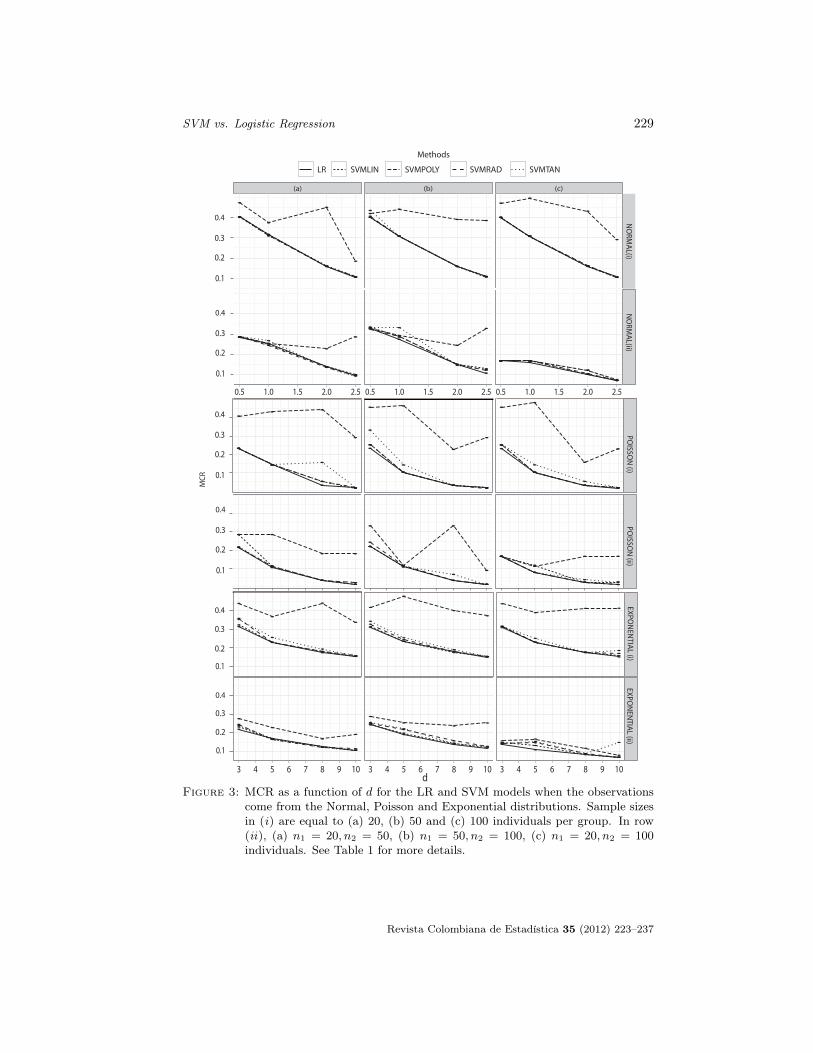
SVM vs. Logistic Regression 229
0.1
0.2
0.3
0.4
(a)
0.5 1.0 1.5 2.0 2.5
(b)
0.5 1.0 1.5 2.0 2.5
(c)
0.5 1.0 1.5 2.0 2.5
0.1
0.2
0.3
0.4
0.1
0.2
0.3
0.4
0.1
0.2
0.3
0.4
d3 4 5 6 7 8 9 10 3 4 5 6 7 8 9 10 3 4 5 6 7 8 9 10
0.1
0.2
0.3
0.4
0.1
0.2
0.3
0.4
NO
RMAL(i)
POISSO
N (i)
NO
RMAL(ii)
POISSO
N (ii)
EXPON
ENTIAL (i)
EXPON
ENTIAL (ii)
MCR
Methods
LR SVMLIN SVMPOLY SVMRAD SVMTAN
Figure 3: MCR as a function of d for the LR and SVM models when the observationscome from the Normal, Poisson and Exponential distributions. Sample sizesin (i) are equal to (a) 20, (b) 50 and (c) 100 individuals per group. In row(ii), (a) n1 = 20, n2 = 50, (b) n1 = 50, n2 = 100, (c) n1 = 20, n2 = 100individuals. See Table 1 for more details.
Revista Colombiana de Estadística 35 (2012) 223–237

230 Diego Alejandro Salazar, Jorge Iván Vélez & Juan Carlos Salazar
4.2. Mixture of Distributions
In Figure 4, the MCR for the Cauchy-Normal and Normal-Poisson mixtures ispresented. Regardless the groups’ sample sizes, SVM models perform better thanLR in a Cauchy-Normal mixture. Interestingly, the polynomial kernel performspoorer when the number of individuals in both groups is the same (upper panel),but its performance improves when they are different (lower panel).
(a) (b) (c)
d1 2 3 4 5 1 2 3 4 5 1 2 3 4 5
0.1
0.2
0.3
0.4
0.5
0.1
0.2
0.3
0.4
0.5
0.1
0.2
0.3
0.4
0.1
0.2
0.3
0.4
CA
UC
HY-N
ORM
AL (i)
CA
UC
HY-N
ORM
AL (ii)
NO
RMA
L-POISSO
N (ii)
NO
RMA
L-POISSO
N (i)
MC
R
Methods
LR SVMLIN SVMPOLY SVMRAD SVMTAN
Figure 4: MCR as a function of d for the LR and SVM models when the observationscome from a Cauchy-Normal and a Normal-Poisson mixture distributions.Conventions as in Figure 3. See Table 1 for more details.
In the Normal-Poisson mixture, the MCRs for SVM are lower than those forLR, especially when d is low, i.e., the expected value of both groups is similar.When n1 = n2 (upper panel), the linear and radial SVM models present lowerMCRs than LR when the sample sizes increase.
Results for the Bivariate Normal distribution are presented in Figure 5. Forall methods, the MCR decreases when ρ increases and the sample size is the same
Revista Colombiana de Estadística 35 (2012) 223–237

SVM vs. Logistic Regression 231
for both groups. However, if the number of individuals per group is different andd is low, the MCR for LR is similar regardless ρ. Under this scenario, the radialand tangential SVM models perform as good as LR. Conversely, the linear kernelshows a poor performance.
ρ
0.1
0.2
0.3
0.4
0.5
0.1
0.2
0.3
0.4
0.5
0.1
0.2
0.3
0.4
0.5
0.1
0.2
0.3
0.4
0.5
0.1
0.2
0.3
0.4
0.5
0.1
0.2
0.3
0.4
0.5
(a)
0.2 0.4 0.6 0.8
(b)
0.2 0.4 0.6 0.8
(c)
0.2 0.4 0.6 0.8
(d)
0.2 0.4 0.6 0.8
Methods
LR SVMLIN SVMPOLY SVMRAD SVMTAN
MCR
(20 , 20)(50 , 50)
(100 ,100)(20 , 50)
(50 , 100)(20 , 100)
Figure 5: MCR as a function of ρ for the Bivariate Normal distribution when the meanvector is (a) (0,0), (b) (1,0), (c) (1, 1.5) and (d) (2.5, 0). Rows correspondto combinations of n1 and n2 of the form (n1, n2). Here (20, 50) correspondsto n1 = 20 and n1 = 50.
Revista Colombiana de Estadística 35 (2012) 223–237

232 Diego Alejandro Salazar, Jorge Iván Vélez & Juan Carlos Salazar
5. Application
Mootha, Lindgren, Eriksson, Subramanian, Sihag, Lehar, Puigserver, Carlsson,Ridderstrele, Laurila, Houstis, Daly, Patterson, Mesirov, Golub, Tamayo, Spiegel-man, Lander, Hirschhorn, Altshuler & Groop (2003) introduce an analytical strat-egy for detecting modest but coordinate changes in the expression of groups offunctionally related genes, and illustrate it with DNA microarrays measuring geneexpression levels in 43 age-matched skeletal muscle biopsy samples from males, 17with normal glucose tolerance (NGT), 8 with impaired glucose tolerance (IGT)and 18 with type 2 diabetes (T2D). As a result, they identified a set of genesinvolved in oxidative phosphorylation.
Table 2: Statistics for the top 10 differentially expressed genes. No correction by mul-tiple testing was applied.
Gene t-statistic xNGT − xT2D P -valueG557 3.8788 0.1632 0.0005G591 −3.6406 −0.1008 0.0009G226 3.0621 0.1285 0.0044G718 −3.0566 −0.1093 0.0044G45 −2.8978 −0.1275 0.0066G137 2.8432 0.1255 0.0076G737 −2.6544 −0.1947 0.0121G587 −2.5774 −0.2654 0.0146G232 −2.5607 −0.3213 0.0152G185 −2.5368 −0.2752 0.0161
For analysis, expression levels were processed as follows. First, a subset of 1000genes was randomly selected from the original data. Second, the expression levelsin samples from NGT (controls, group 1) and T2D individuals (cases, group 2) werecompared using a two-sample t-test as implemented in genefilter (Gentleman,Carey, Huber & Hahne 2011). Third, only the expression levels for the top 30differentially expressed (DE) genes were subsequently used to fit the LR and SVMmodels.
Summary statistics for the top 10 genes found to be DE are presented in Table2; genes G557, G226 and G137 are down-regulated, i.e., their expression levelsare lower in T2D than in NGT samples. Figure 6 depicts a scatterplot for thetop 5 genes by disease status. In there, some (expected) correlation structures areobserved; these correlations might constitute a potential problem for any classifi-cation method.
LR and SVM models were fitted using the disease status as dependent variableand the expression levels of k genes as covariates. Our findings are reported inFigure 7. For predicting the disease status in this data set, (i) SVM modelsrequired less variables (genes); (ii) all methods performed similarly when k <5, but the radial SVM model is more consistent, and (iii) the polynomial andtangential SMVs are definitely not an option. These results may provide importantinsights in the diagnosis of genetic diseases using this type of models.
Revista Colombiana de Estadística 35 (2012) 223–237

SVM vs. Logistic Regression 233
G557
2.90 3.00 3.10 3.20 2.8 2.9 3.0 3.1 3.2
2.6
2.7
2.8
2.9
3.0
3.1
3.2
2.902.953.003.053.103.153.20 G591
G226
2.6
2.7
2.8
2.9
3.0
3.1
3.2
2.6 2.8 3.0 3.2
2.8
2.9
3.0
3.1
3.2
2.6 2.8 3.0 3.2
G718
Figure 6: Scatterplot matrix for some of the genes presented in Table 2. Filled dotscorrespond to NGT samples (controls). In the diagonal panel, density plotsare shown.
Although in our application we only used a subset of the genes available inthe microarray experiment, it illustrates how a SVM model can be used to predictthe (disease) status of a patient using his/her genetic information. Furthermore,we evaluated the possibility of including “one-gene-at-the-time” and determine theMCR of the (full) SVM model as more genetic profiles were added. Using a similarstrategy and by combining SVM with other classification methods such as geneticalgorithms, several authors have been able to build accurate predictive modelsthat, in the near future, could be used to diagnose patients in the clinical setting.Some examples include the work by David & Lerner (2005) in genetic syndromediagnosis, and Furey, Cristianini, Duffy, Bednarski, Schummer & Haussler (2000),Peng, Xum, Bruce Ling, Peng, Du & Chen (2003), and Li, Jiang, Li, Moser, Guo,Du, Wang, Topol, Wang & Rao (2005) in cancer.
SVM models have shown to be highly accurate when cancer diagnosis is ofinterest and either microarray expression data (Furey et al. 2000, Noble 2006)or tumor marker detection (TMD) results for colorectal, gastric and lung cancer(Wang & Huan 2011) are available. For instance, Furey et al. (2000) used 6817gene expression measurements and fitted a SVM model that achieved near-perfectclassification accuracy on the ALL/AML data set (Golub, Slonim, Tamayo, Huard,
Revista Colombiana de Estadística 35 (2012) 223–237

234 Diego Alejandro Salazar, Jorge Iván Vélez & Juan Carlos Salazar
0 5 10 15 20 25 30
0.00
0.05
0.10
0.15
0.20
0.25
0.30
Number of differentially expressed genes
MC
R
LRLinearPolynomialRadialTangential
Figure 7: MCR as a function of the number of differentially expressed genes.
Gaasenbeek, Mesirov, Coller, Loh, Downing, Caligiuri, Bloomfield & Lander 1999).For TMD, Wang & Huan (2011) created, trained, optimized and validated SVMmodels that resulted to be highly accurate compared to others, indicating a po-tential application of the method as a diagnostic model in cancer. Similarly, Penget al. (2003) combined genetic algorithms and paired SVM for multiclass canceridentification to narrow a set of genes to a very compact cancer-related predictivegene set; this method outperformed others previously published.
6. Conclusions
We have presented a framework to compare, by statistical simulation, the per-formance of several classification methods when individuals belong to one of twomutually exclusive categories. As a test case, we compared SVM and LR.
When it is of interest to predict the group to which a new observation belongs tobased on a single variable, SVM models are a feasible alternative to RL. However,as shown for the Poisson, Exponential and Normal distributions, the polynomialSVM model is not recommended since its MCR is higher.
In the case of multivariate and mixture of distributions, SVM performs betterthan LR when high correlation structures are observed in the data (as shown inFigure 6). Furthermore, SVM methods required less variables than LR to achievea better (or equivalent) MCR. This latter result is consistent with Verplancke et al.(2008).
Revista Colombiana de Estadística 35 (2012) 223–237

SVM vs. Logistic Regression 235
Further work includes the evaluation of the MCR of SVM and LR methodsfor other probability distributions, different variance-covariance matrices amonggroups, and high-dimensional (non) correlated data with less variables than ob-servations, e.g., genetic data with up to 5 million genotypes and ∼ 1000 cases andcontrols.
Acknowledgements
DAS and JCS were supported by Programa Nacional de Investigación en Genó-mica, Bioinformática y Estadística para Estudios en Enfermedades Neurosiquiátri-cas. Fase I: Enfermedad de Alzheimer, código 9373, Grupo de Neurociencias dela Universidad Nacional de Colombia, Sede Bogotá. We thank two anonymousreviewers for their helpful comments and suggestions.
[Recibido: septiembre de 2011 — Aceptado: febrero de 2012
]
References
Anderson, T. (1984), An Introduction to Multivariate Statistical Analysis, JohnWiley & Sons, New York.
Asparoukhova, K. & Krzanowskib, J. (2001), ‘A comparison of discriminant proce-dures for binary variables’, Computational Statistics & Data Analysis 38, 139–160.
Cornfield, J. (1962), ‘Joint dependence of the risk of coronary heart disease onserum cholesterol and systolic blood pressure: A discriminant function anal-ysis’, Proceedings of the Federal American Society of Experimental Biology21, 58–61.
Cortes, C. & Vapnik, V. (1995), ‘Support-vector networks’, Machine Learning20(3), 273–297.
Cover, T. M. (1965), ‘Geometrical and statistical properties of systems of linearinequalities with applications in pattern recognition’, IEEE Transactions onElectronic Computers 14, 326–334.
Cox, D. (1966), Some Procedures Associated with the Logistic Qualitative ResponseCurve, John Wiley & Sons, New York.
David, A. & Lerner, B. (2005), ‘Support vector machine-based image classificationfor genetic syndrome diagnosis’, Pattern Recognition Letters 26, 1029–1038.
Day, N. & Kerridge, D. (1967), ‘A general maximum likelihood discriminant’,Biometrics 23, 313–323.
Revista Colombiana de Estadística 35 (2012) 223–237

236 Diego Alejandro Salazar, Jorge Iván Vélez & Juan Carlos Salazar
Dimitriadou, E., Hornik, K., Leisch, F., Meyer, D., &Weingessel, A. (2011), e1071:Misc Functions of the Department of Statistics (e1071), TU Wien. R packageversion 1.5-27.*http://CRAN.R-project.org/package=e1071
Fisher, R. (1936), ‘The use of multiple measurements in taxonomic problems’,Annual Eugenics 7, 179–188.
Furey, T. S., Cristianini, N., Duffy, N., Bednarski, D. W., Schummer, M. & Haus-sler, D. (2000), ‘Support vector machine classification and validation of cancertissue samples using microarray expression data’, Bioinformatics 16(10), 906–914.
Gentleman, R., Carey, V., Huber, W. & Hahne, F. (2011), Genefilter: Methodsfor filtering genes from microarray experiments. R package version 1.34.0.
Golub, T., Slonim, D., Tamayo, P., Huard, C., Gaasenbeek, M., Mesirov, J., Coller,H., Loh, M., Downing, J., Caligiuri, M., Bloomfield, C. & Lander, E. (1999),‘Molecular classification of cancer: Class discovery and class prediction bygene expression monitoring’, Science 286, 531–537.
Hernández, F. & Correa, J. C. (2009), ‘Comparación entre tres técnicas de clasi-ficación’, Revista Colombiana de Estadística 32(2), 247–265.
Hosmer, D. & Lemeshow, S. (1989), Applied Logistic Regression, John Wiley &Sons, New York.
Karatzoglou, A., Meyer, D. & Hornik, K. (2006), ‘Support vector machines in R’,Journal of Statistical Software 15(8), 267–73.
Lee, J. B., Park, M. & Song, H. S. (2005), ‘An extensive comparison of recentclassification tools applied to microarray data’, Computational Statistics &Data Analysis 48, 869–885.
Li, L., Jiang, W., Li, X., Moser, K. L., Guo, Z., Du, L., Wang, Q., Topol, E. J.,Wang, Q. & Rao, S. (2005), ‘A robust hybrid between genetic algorithmand support vector machine for extracting an optimal feature gene subset’,Genomics 85(1), 16–23.
Moguerza, J. & Muñoz, A. (2006), ‘Vector machines with applications’, StatisticalScience 21(3), 322–336.
Mootha, V. K., Lindgren, C. M., Eriksson, K. F., Subramanian, A., Sihag, S.,Lehar, J., Puigserver, P., Carlsson, E., Ridderstrele, M., Laurila, E., Houstis,N., Daly, M. J., Patterson, N., Mesirov, J. P., Golub, T. R., Tamayo, P.,Spiegelman, B., Lander, E. S., Hirschhorn, J. N., Altshuler, D. & Groop, L. C.(2003), ‘Pgc-1α-responsive genes involved in oxidative phosphorylation arecoordinately downregulated in human diabetes’, Nature Genetics 34(3), 267–73.
Revista Colombiana de Estadística 35 (2012) 223–237

SVM vs. Logistic Regression 237
Noble, W. (2006), ‘What is a support vector machine?’, Nature Biotechnology24(12), 1565–1567.
Peng, S., Xum, Q., Bruce Ling, X., Peng, X., Du, W. & Chen, L. (2003), ‘Molecularclassification of cancer types from microarray data using the combination ofgenetic algorithms and support vector machines’, FEBS Letters 555, 358 –362.
R Development Core Team (2011), R: A Language and Environment for StatisticalComputing, R Foundation for Statistical Computing, Vienna, Austria. ISBN3-900051-07-0.*http://www.R-project.org/
Salazar, D. (2012), Comparación de Máquinas de Soporte vectorial vs. RegresiónLogística: cuál es más recomendable para discriminar?, Tesis de Maestría,Escuela de Estadística, Universidad Nacional de Colombia, Sede Medellín.
Shou, T., Hsiao, Y. & Huang, Y. (2009), ‘Comparative analysis of logistic regres-sion, support vector machine and artificial neural network for the differentialdiagnosis of benign and malignant solid breast tumors by the use of three-dimensional power doppler’, Korean Journal of Radiology 10, 464–471.
Tibshirani, R. & Friedman, J. (2008), The Elements of Statistical Learning,Springer, California.
Verplancke, T., Van Looy, S., Benoit, D., Vansteelandt, S., Depuydt, P., De Turck,F. & Decruyenaere, J. (2008), ‘Support vector machine versus logistic regres-sion modeling for prediction of hospital mortality in critically ill patients withhaematological malignancies’, BMC Medical Informatics and Decision Mak-ing 8, 56–64.
Wang, G. & Huan, G. (2011), ‘Application of support vector machine in cancerdiagnosis’, Med. Oncol. 28(1), 613–618.
Westreich, D., Lessler, J. & Jonsson, M. (2010), ‘Propensity score estimation:Neural networks, support vector machines, decision trees (CART), and meta-classifiers as alternatives to logistic regression’, Journal of Clinical Epidemi-ology 63, 826–833.
Revista Colombiana de Estadística 35 (2012) 223–237

Revista Colombiana de Estadística
Número especial en Bioestadística
Junio 2012, volumen 35, no. 2, pp. 239 a 254
¿Cuándo inicia la enfermedad de Alzheimer?
Kaplan-Meier versus Turnbull: una aplicación a
datos con censura arbitraria
¿When does Alzheimer’s Disease Begin? Kaplan-Meier versus
Turnbull: An Application to Arbitrary Censoring Data
Carlos Mario Lopera-Gómez1,a, Mario César Jaramillo-Elorza1,b,
Natalia Acosta-Baena2,c
1Escuela de Estadística, Facultad de Ciencias, Universidad Nacional de Colombia,
Medellín, Colombia
2Grupo de Neurociencias de Antioquia y Grupo Académico de Epidemiología
Clínica-GRAEPIC, Facultad de Medicina, Universidad de Antioquia, Medellín,
Colombia
Resumen
La mayoría de los análisis de supervivencia se basan en tiempos de fallaexactos y observaciones censuradas a la derecha, utilizándose métodos am-pliamente difundidos como el método de Kaplan-Meier (KM). Para estimarla edad de inicio de la Enfermedad de Alzheimer (EA) familiar cuando lascensuras son arbitrarias (censura a derecha, a izquierda o en intervalo), ¿cuáles el cambio en los resultados clínicos, si se utiliza el método de KM medianteimputación comparado con el método de Turnbull sugerido para este tipo dedatos?
El método de Turnbull se comparó con el método de KM mediante unestudio de simulación y una aplicación con datos reales. Se realizó KM conimputación a través del punto medio del intervalo (PM) y en el extremo dere-cho (ED). Se analizaron diferentes tamaños de muestra y diferentes tiemposentre visitas.
En todos los escenarios de simulación, las funciones que fueron estima-das, usando imputación de datos, difieren significativamente de la verdaderafunción de supervivencia S(t).
La edad de inicio de la EA determinada a través de un método de impu-tación tiene implicaciones clínicas relevantes que afectarían la toma de de-cisiones a la hora de iniciar una terapia preventiva. El método de Turnbull
aProfesor asistente. E-mail: [email protected] asociado. E-mail: [email protected]. E-mail: [email protected]
239
240 Carlos Mario Lopera-Gómez, et al.
presenta un menor sesgo cuando se necesita realizar un análisis de supervi-vencia con censuras arbitrarias.
Palabras clave: análisis de supervivencia, censura de intervalo, edad deinicio, enfermedad de Alzheimer familiar.
Abstract
Most of the survival analysis are based on exact failure times and rightcensored observations, using methods widely known as the Kaplan-Meier(KM). To estimate the onset age of familial Alzheimer’s Disease (AD) whenthe censor times are arbitrary (right, left or interval censor), what is thechange in clinical outcomes, using the KM method with data imputationcompared with procedure proposed by Turnbull for this kind of data?
Turnbull’s method was compared with KM method in a simulation studyand an application with real data. KM method was based on data imputationthrough the midpoint of the interval (MP) and the right side of the interval(RS), considering several sample sizes and different times between visits.
In all simulation scenarios estimated functions using data imputationdiffer significantly from the actual simulated survival function S(t).
The estimated onset age of AD through data imputation methods hasrelevant clinical implications that would affect decision-making in initiatingpreventive therapy. Turnbull’s method has fewer bias when was comparedwith KM with imputation to perform a survival analysis with arbitrary cen-sure data.
Key words: Age of onset, Familial Alzheimer’s disease, Interval censoring,Survival analysis.
1. Introducción
El análisis de supervivencia es un conjunto de procedimientos estadísticos para
el análisis de datos en los que la variable de resultado es el tiempo hasta que
ocurre un evento de interés. La función de supervivencia es quizás la función más
importante en los estudios de medicina y salud. Como es usual en el análisis de
datos de supervivencia, es de interés estimar la función de supervivencia S(t)y evaluar la importancia de factores potenciales de pronóstico o características
individuales sobre este tiempo de supervivencia.
La gran cantidad de estudios epidemiológicos realizados en enfermedades co-
mo el cáncer, entre muchas otras, y la cantidad de estudios longitudinales con
desenlaces que involucran el tiempo demuestran la importancia del análisis de
supervivencia. Alternativamente al desenlace de supervivencia o tiempo hasta la
muerte, el tiempo puede hacer referencia al momento en que una persona presenta
cualquier otro evento. Si el evento se presenta en todos los individuos, se podrían
aplicar muchos métodos. Sin embargo, lo habitual es que al final del seguimiento
algunas de las personas no han desarrollado el evento de interés, por lo que el
verdadero tiempo trascurrido hasta el evento es no observado. Además, los datos
de supervivencia rara vez se distribuyen de forma “normal”, y se componen ge-
neralmente de muchos eventos al inicio del seguimiento, y los eventos tardíos son
Revista Colombiana de Estadística 35 (2012) 239–254
¿Cuándo inicia la enfermedad de Alzheimer? 241
relativamente pocos. Estas características de los datos son las que hacen necesario
un método especial como el análisis de supervivencia.
Las dificultades específicas relacionadas con el análisis de supervivencia surgen
en gran medida por el hecho de que sólo algunas personas han experimentado el
evento; por lo tanto, el tiempo de supervivencia se desconoce en un subconjunto
de sujetos del estudio. Este fenómeno se llama censura y sus mecanismos pueden
deberse a que el individuo no ha experimentado el desenlace en el momento de
cierre del estudio; porque se pierde del seguimiento: o porque el sujeto presenta un
evento diferente que hace imposible un seguimiento posterior (riesgo competitivo).
En este último caso, las censuras deben estimarse de manera distinta y requiere
un análisis especial de los datos. Pero al visualizar el proceso de supervivencia
de un individuo como una línea de tiempo pueden verse tres tipos de censuras:
si el evento (suponiendo que llegara a ocurrir) está más allá del final del período
de seguimiento, esta situación se conoce como censura a derecha. Otro caso se
presenta cuando se observa el evento de interés antes de la primera evaluación,
pero no se sabe exactamente cuándo ocurrió. Este tipo de censura es la censura
a izquierda. Y por último, el tiempo trascurrido hasta el evento también puede
ser censurado en intervalo; cuando los individuos salen y entran del seguimiento
(por ejemplo, cuando los individuos se presentan a controles médicos con cierta
frecuencia), el individuo presenta el evento de interés al regreso del seguimiento
pero la única información que se tiene en este caso, es que el evento se produce
dentro de un intervalo de tiempo dado.
La mayoría de los datos de supervivencia incluyen solo observaciones censu-
radas a derecha y tiempos de falla exactos, utilizándose métodos ampliamente
difundidos como el método de Kaplan-Meier (KM), pruebas de logrank y regre-
sión de Cox (análisis de riesgos proporcionales). Sin embargo, los métodos que
soportan datos censurados a izquierda o en intervalo no son tan conocidos. Pocos
paquetes estadísticos permiten estos datos, y por esta razón, la práctica común
entre los investigadores consiste en simplemente ignorar y descartar las censuras
a izquierda de los datos, o realizar una imputación del desenlace para las censuras
de intervalo. Es decir, asumir que el evento que ha ocurrido dentro del intervalo
(Li, Ui] ocurrió ya sea en el límite inferior o superior del intervalo o en el punto
medio del mismo. Autores como Rucker & Messerer (1988), Odell, Anderson &
D’agostinho (1992), Dorey, Little & Schenker (1993) y Iceland (1997) manifiestan
que asumir el tiempo de supervivencia de intervalo como si fuera exacto puede
conducir a estimadores sesgados, así como a conclusiones y estimaciones parcia-
les que no son completamente fidedignas. Estas afirmaciones motivan, de alguna
manera, a propuestas distintas relacionadas con el tratamiento que se debe dar a
estas censuras, con el fin de evitar sesgos y que se incorpore mayor información.
Los datos de la Cohorte Antioquia-E280A de 15 años de seguimiento, con
sujetos en riesgo de enfermedad de Alzheimer familiar, incluyen los tres tipos de
censuras mencionadas previamente. Conocer la edad de inicio de la enfermedad en
estos sujetos que inevitablemente van a desarrollar la Enfermedad de Alzheimer
(EA) exige métodos alternativos para dicha estimación. En este estudio se pretende
difundir tales métodos e ilustrar qué tan erróneas serían las estimaciones en la
edad de inicio de la EA, utilizando el método KM comparado con el método
Revista Colombiana de Estadística 35 (2012) 239–254
242 Carlos Mario Lopera-Gómez, et al.
de Turnbull para estimación bajo censura arbitraria (Peto 1973, Turnbull 1974,
Turnbull 1976). También interesa determinar las implicaciones desde el punto de
vista clínico cuando se incurre en un sesgo de medición y la importancia de los
resultados para el diagnóstico del inicio de la EA familiar. Inicialmente se realiza
un estudio de simulación y posteriormente la aplicación con los datos reales.
En la sección 2 se presenta el problema clínico y la base de datos que servirá
para ilustrar los métodos que van a ser comparados. Los métodos estadísticos
utilizados y el planteamiento de un estudio de simulación son presentados en la
sección 3. La sección 4 recopila los resultados obtenidos a través del estudio de
simulación y presenta la aplicación con los datos de enfermedad de Alzheimer.
Finalmente, en la sección 5 se dan algunas conclusiones y recomendaciones con
base en los hallazgos encontrados.
2. Problema y datos de enfermedad de Alzheimer
Conocer el tiempo hasta el inicio de la enfermedad de Alzheimer sólo es po-
sible gracias a las formas genéticas de la enfermedad, con herencia autosómica
dominante. En esta condición, todos los sujetos nacen portando una mutación que
predispone a la enfermedad, expresándose en algún momento de la vida. Las ma-
nifestaciones consisten en quejas de memoria y deterioro cognitivo evidente en las
evaluaciones neurosicológicas alrededor de los 50 años de edad. Conocer la edad
más aproximada del inicio de la enfermedad es el primer paso para planear y desa-
rrollar nuevos estudios en busca de terapias preventivas. El Grupo de Neurociencias
de la Universidad de Antioquia ha seguido desde 1995 a este conglomerado pobla-
cional, que es el más numeroso del mundo, con 5000 sujetos estimados, con riesgo
de desarrollar EA genético mutación E280A en Presenilina 1 (PSEN1). Se identi-
ficaron, hasta enero del 2010, 1784 sujetos pertenecientes a 25 familias afectadas.
Se detectaron 449 sujetos portadores de la mutación E280A-PSEN1. Los datos
de estos últimos sujetos portadores fueron los utilizados para detectar el inicio de
la enfermedad de manera retrospectiva (Acosta-Baena, Sepúlveda-Falla, Lopera-
Gómez, Jaramillo-Elorza, Moreno, Aguirre-Acevedo, Saldarriaga & Lopera 2011).
3. Métodos
Con base en los datos descritos en la sección 2, se utilizaron los métodos de
imputación, para comparar la función de supervivencia de Turnbull con KM.
Para medir la edad de inicio de la enfermedad, se realizó un análisis de supervi-
vencia evaluando el tiempo transcurrido desde la fecha de nacimiento hasta la fecha
de aparición del deterioro cognitivo leve o hasta la fecha de la última evaluación. Se
utilizó el método de supervivencia desarrollado por Peto (1973), Turnbull (1974)
y Turnbull (1976), que incluye los tres tipos de censuras, mediante el algoritmo
implementado por Giolo (2004), para el software R versión 2.13.1 (R Development
Core Team 2011). El código utilizado hace uso de la librería SURVIVAL del software
R, y está disponible bajo pedido a los autores.
Revista Colombiana de Estadística 35 (2012) 239–254

¿Cuándo inicia la enfermedad de Alzheimer? 243
3.1. Estimador no paramétrico de Turnbull
En los estudios longitudinales, donde los individuos son monitoreados durante
un lapso de tiempo prefijado, o visitados periódicamente un cierto número de
veces, el tiempo Ti, i = 1, . . . , n, hasta que ocurre el evento de interés para cada
individuo, se desconoce. Sólo se sabe que está dentro de un intervalo entre dos
visitas, es decir, entre la visita en el tiempo Li y la visita en el tiempo Ui con
Li < Ti ≤ Ui. Si el evento ocurre exactamente en el momento de una visita, lo
cual es muy poco probable, pero puede ocurrir, se tiene un tiempo de supervivencia
exacto. En este caso se asume que Li = Ti = Ui.
Por otra parte, se sabe que para los individuos cuyos tiempos están censurados
a derecha, el evento de interés no ha ocurrido hasta la última visita, pero puede
ocurrir en cualquier instante desde ese momento en adelante. Por consiguiente, se
supone en este caso que Ti puede ocurrir dentro del intervalo (Li,+∞), con Li
igual al periodo desde el comienzo del estudio hasta la última visita y Ui = +∞.
De modo semejante, para los individuos cuyos tiempos están censurados a
izquierda, se sabe que el evento de interés ha ocurrido antes de la primera visita,
y, por lo tanto, suponemos que Ti ha ocurrido en el intervalo (0, Ui], con Li = 0representando el comienzo del estudio, y Ui es el tiempo hasta la primera visita. El
método de Turnbull generaliza cualquier situación con combinaciones de tiempos
de supervivencia (exacto o intervalo) y censuras a izquierda y derecha como datos
de supervivencia de intervalo. Por lo tanto, los tiempos de supervivencia exacta, así
como datos de censura a izquierda y derecha, son todos casos especiales de datos
de supervivencia con censura de intervalo con Li = Ui para censuras exactas,
Ui = +∞ para las censuras a derecha y Li = 0 para censuras a izquierda.
Como uno de los objetivos principales en análisis de supervivencia es estimar
la función de supervivencia e investigar la importancia de factores potenciales de
pronóstico bajo tiempos de supervivencia con censura a intervalo, el número de
factores bajo estudio debería depender del propósito del estudio. Como lo sugiere
Hougaard (1999), la estimación no paramétrica de la función de distribución acu-
mulada F (t), o en su defecto de la función de supervivencia S (t), es preferible a
su estimación paramétrica, por varias razones. Por ejemplo, una elección equivo-
cada de la distribución paramétrica de T podría conducir a conclusiones erróneas
de S (t). Además, podría ser difícil encontrar una distribución paramétrica apro-
piada para ajustar los datos. Hougaard da el ejemplo de tiempos de vida de una
población cuya función hazard muestra la llamada forma de bañera: la cual en un
principio decrece pocos años, luego permanece constante durante muchos años y
por último empieza a aumentar. En este caso, el mejor ajuste probablemente se
obtendría de una mezcla de distribuciones.
En el caso de censura a derecha, se podría usar el estimador de Kaplan-Meier
para obtener S (t) (Kaplan & Meier 1958). Sin embargo, con datos censurados
en intervalo, el método de Kaplan-Meier no puede ser aplicado, y han sido Peto
(1973), Turnbull (1974) y Turnbull (1976) quienes han desarrollado el estimador
no paramétrico de máxima verosimilitud (NPMLE, por su sigla en inglés) para
estos datos.
Revista Colombiana de Estadística 35 (2012) 239–254
244 Carlos Mario Lopera-Gómez, et al.
El estimador de Turnbull, se basa en una muestra de intervalos observados
[Li, Ri] , i = 1, . . . , n, los cuales contienen las variables aleatorias independientes
T1, . . . , Tn. Como se mencionó antes, una observación exacta de Ti se da sólo si
Li = Ri.
Dado este ejemplo, la función de verosimilitud a ser maximizada es la siguiente:
L (F ) =
n∏
i=1
[F (Ri+)− F (Li−)] (1)
Para resolver este problema de maximización, Peto (1973) define dos conjun-
tos γ = Li, i = 1, . . . , n y κ = Ri, i = 1, . . . , n que contienen los extremos
izquierdos y derechos de los intervalos, respectivamente. Si se denotan los incre-
mentos de la función F dentro de los intervalos [qj , pj ] como sj, j = 1, . . . ,m,
entonces L (F ) debe ser maximizada como una función de s1, s2, . . . , sm, sujeto
a las restricciones sj ≥ 0 y sm = 1 −∑m−1
j=1 sj . Peto aborda este problema de
maximización usando el algoritmo de Newton-Raphson.
Se puede probar que una función que maximice (1) es constante entre los inter-
valos [qj , pj ] e indefinida dentro de ellos. Note que esto implica que P (T ∈ (pj−1,
qj)) = 0 para cualquier j. Como la función de distribución es no decreciente,
la cual no es constante entre los intervalos, puede no maximizar a L (F ). De-
note los incrementos de F dentro de los intervalos [qj , pj ] por sj j = 1, . . . ,m,
L (F ) debe ser maximizada como una función de s1, s2, . . . , sm sujeto a sj ≥ 0 y
sm = 1−m−1∑j=1
sj . Peto aborda este problema de maximización usando el algoritmo
de Newton-Raphson. En contraste con Peto, Turnbull (1976) propone el uso del
algoritmo de auto-consistencia para el mismo problema de maximización. La idea
de este algoritmo fue presentada primero por Efron (1967), y su aplicación para
la maximización en (1) es como sigue.
Sea αij = I[qj ,pj ]∈[Li,Ri], i = 1, . . . , n, j = 1, . . . ,m, las variables indicadoras
que confirman si el intervalo [qj , pj ] se encuentra dentro o no del intervalo [Li, Ri];entonces, la probabilidad de que Ti se encuentre dentro del intervalo [qj , pj ] dado
un vector s = (s1, s2, . . . , sm)′ está dada por:
µij (s) =αijsj
m∑k=1
αiksk
(2)
puesto que F es constante fuera de los intervalos [qj , pj ]. La proporción de obser-
vaciones en el intervalo [qj , pj] es igual a:
πj (s) =1
n
n∑
i=1
µij (s) (3)
y un vector s = (s1, s2, . . . , sm)′es llamado auto-consistente, si
sj = πj (s) , j = 1, . . . ,m
Revista Colombiana de Estadística 35 (2012) 239–254

¿Cuándo inicia la enfermedad de Alzheimer? 245
Siguiendo esta definición, el algoritmo de auto-consistencia de Turnbull para
el cálculo del estimador no paramétrico de F (t) se puede implementar siguiendo
estos pasos:
1. Obtenga estimaciones iniciales de s; por ejemplo, s(0)j = 1
m, j = 1, . . . ,m.
2. Para i = 1, . . . , n, j = 1, . . . ,m, calcule µij
(s(0)
)acorde a (2), y luego
πj
(s(0)
)de acuerdo a (3).
3. Obtenga estimaciones mejoradas para s hallando s(1)j = πj
(s(0)
).
4. Retorne al paso 2, reemplazando s(0) por s
(1) y continúe hasta que se logre
la convergencia.
3.2. Estudio de simulación
Para establecer el efecto de la imputación de fallas exactas cuando en realidad
se tiene una censura a intervalo, sobre la estimación de la función de supervivencia
se utilizarán datos de falla lognormales con parámetros fijos para la simulación en
valores µ = 3.78419 y σ = 0.133, que se escogieron de tal forma que se emulan
las condiciones de falla de los individuos presentes en el estudio de EA descrito
en la sección 2 (tales valores son una estimación paramétrica de datos de fallas
exactas generados de la función de supervivencia estimada mediante Turnbull,
con el método de la transformación inversa de probabilidad integral; Kalbfleisch
(1985)).
Se asume un punto de partida aleatorio para que el individuo comience sus visi-
tas al estudio, en donde se registrará si éste tiene o no el evento. Así, se construyen
intervalos de tiempo de una de las siguientes formas:
• (0, Ui] un individuo llegó al estudio en el tiempo Ui pero ya tenía el evento de
interés (esto constituye una censura a izquierda, la cual se puede ver como
una censura a intervalo),
• (Li, Ui] un individuo llegó al estudio y asistió a visitas regulares, y en el
tiempo Li fue la última visita en la cual no tenía el evento pero al volver
en la siguiente visita (al tiempo Ui = Li + TEV, con TEV: el tiempo entre
visitas) el individuo ya tiene el evento de interés (esto también constituye
una censura a intervalo), y
• (Li,+∞) un individuo llegó al estudio, asistió a varias visitas regulares, y en
el tiempo Li fue la última visita de la que se tiene registro del individuo en el
estudio, sin que éste haya presentado el evento (esto constituye una censura
a derecha).
Con este esquema de datos, no se tienen tiempos de falla exactos (aunque
también las fallas exactas se pueden considerar como censuras a intervalo con
Li = Ui) y todos los datos deben entrarse al análisis como intervalos de tiempo.
Los factores de simulación que se van a variar son:
Revista Colombiana de Estadística 35 (2012) 239–254
246 Carlos Mario Lopera-Gómez, et al.
1. Método de imputación (MI): de acuerdo a la literatura se estudiarán los
casos en que las censuras de intervalo son imputadas a través del punto
medio del intervalo (PM) y utilizando el extremo derecho del mismo (ED).
Lo cual lleva a tiempos de falla “exactos” y facilita los análisis, ya que la
estimación de Kaplan-Meier (KM) para la curva de supervivencia puede ser
estimada. Además, se considera el caso en que ninguna imputación es llevada
a cabo (NI), es decir, usando los datos en forma de intervalos de tiempo, lo
cual necesariamente lleva a utilizar el estimador de Turnbull (TB) para la
función de supervivencia que tiene en cuenta censura arbitraria.
2. Tiempo entre visitas (TEV): indica con qué frecuencia los individuos asisten
a los controles en el estudio. Interesan valores de TEV = 1, 2, 4 y 6 años.
3. Tamaño de la muestra (n): este factor tiene como objetivo establecer el efecto
sobre el proceso de estimación del número de individuos en el estudio. Se
tomarán valores de n = 50, 100, 200, 500.
Se utilizará como control para comparar el desempeño de las estimaciones el
estimador KM, bajo los métodos de imputación “S(t)PM” y “S(t)ED”, y el esti-
mador de Turnbull “S(t)TB”, a la función de supervivencia real, notada “S(t)”.Esto permite, a través de las diferencias observadas entre cada una de las curvas
“S(t)TB”, “S(t)PM” y “S(t)ED”, y la curva de supervivencia de referencia “S(t)”,establecer el efecto de la imputación sobre la estimación.
Para comparar las curvas de supervivencia resultantes de la simulación, se
generan N = 1000 muestras independientes para cada uno de los 16 escenarios de
simulación (resultantes de las combinaciones de los niveles de los factores TEV y n).
Luego, en cada escenario se realizan las estimaciones de la función de supervivencia,
de acuerdo al factor de imputación: S(t)PM, S(t)ED y S(t)TB, y se comparan con
la función de supervivencia de control S(t). Tal comparación se realiza usando
el error cuadrático medio integrado (ECMI) como una medida global de error.
Para calcular el ECMI con N = 1000 simulaciones en cada escenario, se utiliza la
siguiente fórmula:
ECMIi =1
N
N∑
j=1
∫ [Sj (t)i − S (t)
]2dt
donde i = TB,PM,ED representa el método de estimación de la función de super-
vivencia y S(t) es la función de supervivencia real.
Adicionalmente, para establecer dónde se dan las diferencias entre las cur-
vas de supervivencias estimadas con la real, se calculó el error cuadrático medio
(ECM) en la estimación de los cuantiles q0.05, q0.1, q0.25, q0.5, q0.75, q0.9, q0.95,
de manera que se establece el correspondiente sesgo de estimación de los mé-
todos estudiados (TB, ED y PM). El ECM se calculó para i = TB,PM,ED y
h = 0.05, 0.1, 0.25, 0.5, 0.75, 0.9, 0.95 como:
ECMi,h =1
N
N∑
j=1
(qh,i,j − qh)2
Revista Colombiana de Estadística 35 (2012) 239–254

¿Cuándo inicia la enfermedad de Alzheimer? 247
donde qh,i,j son N = 1000 estimaciones en cada uno de los métodos estudiados
i = TB,PM,ED de los cuantiles reales qh, h = 0.05, 0.1, 0.25, 0.5, 0.75, 0.9, 0.95 de
la distribución lognormal con parámetros µ = 3.78419 y σ = 0.133.
4. Resultados
4.1. Estudio de simulación
4.1.1. Diferencias en las funciones de supervivencia
La medida de error que se utiliza para comparar las estimaciones basadas en
imputación S(t)PM, S(t)ED y S(t)TB, con la función de supervivencia verdadera
S(t), es el ECMI definido en la sección anterior. Un valor pequeño del ECMI indica
que el método de estimación correspondiente produce una curva de supervivencia
estimada que es muy cercana a la curva de supervivencia real a lo largo del tiempo;
por el contrario, valores altos del ECMI indican que las curvas comparadas tienen
diferencias a lo largo del tiempo.
La tabla 1 muestra los ECMI obtenidos en cada uno de los 16 escenarios de
simulación considerados.
Tabla 1: ECMI estimado con los métodos TB, PM y ED.
n TEV ECMITB ECMIED ECMIPM
50 1 3.04 42.11 32.51
50 2 2.24 30.25 32.04
50 4 2.50 29.69 31.68
50 6 2.95 34.16 32.06
100 1 1.58 41.45 31.85
100 2 1.18 28.82 31.30
100 4 1.35 29.28 31.53
100 6 1.64 33.21 31.24
200 1 0.87 41.17 30.88
200 2 0.71 28.82 30.63
200 4 0.76 28.64 30.86
200 6 0.96 33.15 30.79
500 1 0.45 40.73 30.78
500 2 0.38 28.31 30.52
500 4 0.42 28.36 30.53
500 6 0.50 32.74 30.62
En todos los escenarios de simulación el ECMI muestra que las funciones esti-
madas S(t)PM y S(t)ED difieren significativamente de S(t), lo cual indica que las
estimaciones basadas en estas curvas pueden estar muy alejadas de la realidad.
Por otro lado, el ECMI asociado a la estimación de Turnbull (S(t)TB) tiene los
valores más pequeños en todos los escenarios, lo cual sucede sin importar el tama-
ño de muestra. Sin embargo, a medida que el tamaño de muestra aumenta, este
error disminuye su valor. En el análisis del tiempo entre visitas (TEV) se puede
observar que hay un patrón consistente en todos los valores del tamaño de muestra
Revista Colombiana de Estadística 35 (2012) 239–254

248 Carlos Mario Lopera-Gómez, et al.
considerados, que indica que TEV= 2 años provoca un ECMI menor que en los
demás valores de TEV.
La figura 1 ilustra uno de los escenarios considerados en el estudio de simu-
lación (n = 500, TEV = 2), donde claramente se observan diferencias entre las
curvas de supervivencia estimadas usando los diferentes métodos de imputación y
la supervivencia real, mientras que la supervivencia estimada mediante Turnbull
se ajusta bien a esta última.
0 20 40 60 80
0.0
0.2
0.4
0.6
0.8
1.0
Comparación de funciones estimadas
Tiempo en años
S(t
)
S(t)
S(t)TB
S(t)ED
S(t)PM
Figura 1: Diferencias entre la curva real y las curvas estimadas mediante Turnbull yKM(ED) y KM(PM). Una realización del caso simulado con n = 500 y TEV= 2.
4.1.2. Diferencias en las edades de inicio
Para el caso ilustrado en la figura 1, se estimaron la edad de inicio y sus respec-
tivos límites de confianza en cada una de las curvas de supervivencia estimadas,
mediante el método bootstrap percentil, lo cual se resume en la tabla 2. Detalles
del proceso de estimación bootstrap se encuentran en Acosta-Baena et al. (2011),
Meeker & Escobar (1998).
Observe que las edades estimadas de inicio de la EA obtenidas por imputación
de datos (PM y ED) difieren significativamente del valor de referencia, mientras
que el método de Turnbull estima bien. Esto se repite en todos los demás escenarios
considerados.
Revista Colombiana de Estadística 35 (2012) 239–254

¿Cuándo inicia la enfermedad de Alzheimer? 249
Tabla 2: Estimaciones de la edad de inicio para datos simulados.
Mediana LI95 % LS95 %
Referencia 44.00000 – –
TB 44.00006 43.00002 44.99997
KM(ED) 51.00004 51.00002 52.00000
KM(PM) 34.00003 33.99999 38.99993
4.1.3. Sesgos de estimación de algunos cuantiles
A continuación se presentan los ECM calculados en los métodos estudiados.
Tabla 3: ECM para las estimaciones de los cuantiles qh, h = 0.05, 0.1, 0.25, 0.5, 0.75,0.9, 0.95, usando el método TB.
n TEV q0.05 q0.1 q0.25 q0.5 q0.75 q0.9 q0.95
50 1 7.34 5.76 4.67 3.96 5.71 9.92 12.96
50 2 6.30 4.54 3.13 2.96 3.72 6.55 9.24
50 4 7.56 5.43 3.72 3.13 3.42 5.86 7.84
50 6 9.24 5.86 4.45 3.96 4.37 6.76 9.67
100 1 3.88 2.92 2.10 2.10 2.66 5.06 7.51
100 2 3.57 2.56 1.61 1.44 1.93 3.42 5.57
100 4 4.16 3.10 2.10 1.66 2.02 3.13 4.84
100 6 5.38 3.65 2.59 2.19 2.37 3.69 5.06
200 1 2.16 1.64 1.14 1.32 1.56 2.59 4.28
200 2 1.99 1.32 0.98 0.98 1.25 1.80 2.89
200 4 2.53 1.72 1.12 1.06 1.25 1.77 2.31
200 6 2.96 2.10 1.49 1.32 1.46 2.07 2.86
500 1 0.94 0.77 0.61 0.66 0.85 1.25 1.72
500 2 0.86 0.74 0.58 0.59 0.59 0.92 1.32
500 4 1.19 0.86 0.64 0.62 0.67 0.94 1.28
500 6 1.44 1.08 0.77 0.69 0.72 1.04 1.37
Note que los sesgos de estimación al utilizar el método TB (tabla 3) son me-
nores que los obtenidos con los métodos de imputación PM y ED (tablas 4 y 5,
respectivamente). En particular, los sesgos de estimación asociados al método de
imputación PM (tabla 4) son mayores en los cuantiles más pequeños, mientras que
para el método de imputación ED (tabla 5) los sesgos mayores se presentan en los
cuantiles más grandes.
Ahora, en general (tablas 3, 4, y 5) observe que a medida que el tamaño de
muestra aumenta, los sesgos medidos con el ECM disminuyen, y que los resultados
señalan que el tiempo óptimo entre visitas sería de dos años, ya que en este caso
los ECM resultaron menores que en los demás valores de este factor.
4.2. Aplicación con datos reales
Para los datos de EA, se aplicaron las diferentes técnicas de estimación de la
función de supervivencia, y con base en ellas se calculó la mediana como estimador
de la edad de inicio de la enfermedad.
Revista Colombiana de Estadística 35 (2012) 239–254

250 Carlos Mario Lopera-Gómez, et al.
Tabla 4: ECM para las estimaciones de los cuantiles qh, h = 0.05, 0.1, 0.25, 0.5, 0.75,0.9, 0.95, usando el método de imputación PM.
n TEV q0.05 q0.1 q0.25 q0.5 q0.75 q0.9 q0.95
50 1 166.67 168.48 139.95 88.55 14.29 14.29 17.81
50 2 166.67 169.00 140.19 85.38 11.42 7.56 11.16
50 4 167.18 169.26 139.00 84.64 13.10 7.90 7.90
50 6 168.22 169.26 139.95 86.49 12.89 7.18 7.62
100 1 165.12 163.58 140.42 88.92 8.70 8.64 12.82
100 2 164.61 164.61 139.95 82.08 9.30 4.33 6.60
100 4 165.12 164.61 139.48 83.17 10.30 4.54 4.41
100 6 164.10 164.10 138.06 80.28 9.86 4.00 3.84
200 1 169.26 166.67 139.95 91.58 5.90 3.92 9.42
200 2 168.48 166.41 140.42 85.93 8.29 2.66 3.24
200 4 167.44 165.64 139.71 86.12 9.30 3.24 2.69
200 6 168.74 165.89 139.95 85.93 8.94 2.96 2.28
500 1 169.78 166.41 139.71 94.67 4.93 1.51 3.61
500 2 169.52 166.15 140.66 89.11 7.84 1.90 1.39
500 4 170.04 166.67 140.19 89.49 8.64 2.59 1.56
500 6 169.52 165.89 140.42 89.30 8.24 2.28 1.25
Tabla 5: ECM para las estimaciones de los cuantiles qh, h = 0.05, 0.1, 0.25, 0.5, 0.75,0.9, 0.95, usando el método de imputación ED.
n TEV q0.05 q0.1 q0.25 q0.5 q0.75 q0.9 q0.95
50 1 23.33 27.56 45.83 102.01 180.63 199.66 176.62
50 2 16.32 16.65 27.98 58.06 135.02 177.69 159.52
50 4 22.28 23.33 32.95 54.17 114.06 157.25 155.75
50 6 27.88 29.92 40.20 64.32 121.66 160.78 156.50
100 1 18.23 22.75 42.51 97.81 183.60 205.92 178.49
100 2 15.29 16.16 26.01 56.40 133.40 181.44 166.41
100 4 20.98 22.75 31.81 53.44 111.94 163.58 158.26
100 6 26.94 30.03 39.94 62.25 117.07 164.61 158.00
200 1 16.08 21.44 40.83 94.67 181.98 207.65 181.98
200 2 13.76 15.60 24.70 54.61 133.86 184.14 170.82
200 4 19.36 21.90 30.80 53.29 111.72 165.64 160.78
200 6 25.00 29.48 39.44 63.36 116.86 167.96 162.05
500 1 15.37 20.70 39.69 94.09 183.87 209.38 183.33
500 2 13.10 15.21 24.30 53.58 132.94 184.42 171.87
500 4 18.75 21.53 30.47 52.85 111.30 167.44 163.58
500 6 24.11 28.73 39.44 62.73 117.29 169.52 163.84
La tabla 6 muestra cómo es la estimación de la edad de inicio de la enfermedad.
Tabla 6: Estimaciones de la edad de inicio para datos de EA.
Mediana LI95 % LS95 %
TB 44.01006 43.01003 45.01003
KM(ED) 47.00998 46.00002 47.99997
KM(PM) 44.00499 42.00502 45.00498
Revista Colombiana de Estadística 35 (2012) 239–254

¿Cuándo inicia la enfermedad de Alzheimer? 251
Los resultados anteriores muestran que las estimaciones que usan TB y PM,
estiman la edad de inicio a los 44 años, mientras que el método ED sobrestima tal
valor. A nivel de intervalos de confianza, el método de Turnbull es más preciso que
el método PM en la estimación de la edad de inicio de la enfermedad.
La figura 2 muestra las diferencias apreciables entre las curvas estimadas.
0 20 40 60 80
0.0
0.2
0.4
0.6
0.8
1.0
Tiempo en años
S(t
)
Curvas estimadas de supervivencia
para la enfermedad de Alzheimer familiar
S(t)TB
S(t)ED
S(t)PM
Figura 2: Funciones de supervivencia estimadas para los datos de EA.
Note que aunque las estimaciones de la edad de inicio que usan TB y PM son
similares, estimaciones de otros cuantiles, particularmente cuantiles más pequeños,
pueden llevar a errores apreciables. Esto puede deberse principalmente a que los
datos de EA familiar incluyen un 21 % de datos con censura a izquierda (Acosta-
Baena et al. 2011).
5. Conclusiones y recomendaciones
• En las últimas décadas existe gran interés en todo el mundo por definir
adecuadamente el inicio de la EA, incluso etapas preclínicas y prodrómicas,
con el objetivo de detectar la enfermedad de manera más temprana y ofre-
cer alternativas de tratamiento más oportuno (Petersen, Stevens, Ganguli,
Tangalos, Cummings & DeKosky 2001, Reisberg, Ferris, Kluger, Franssen,
Wegiel & de Leon 2008). Conocer adecuadamente la edad de inicio de esta
cohorte de portadores de una mutación con irremediable inicio de la enferme-
dad de Alzheimer tiene utilidad para el diseño de ensayos clínicos dirigidos
a tratamientos preventivos (Strobel 2011).
Revista Colombiana de Estadística 35 (2012) 239–254

252 Carlos Mario Lopera-Gómez, et al.
• En los análisis realizados, las edades de inicio de la EA obtenidas por impu-
tación de datos (PM y ED) difieren significativamente de los datos reales
en todos los tamaños de muestra y en los diferentes TEV, mientras que el
método de Turnbull estima bien en todos los escenarios. También puede con-
cluirse que un tiempo entre visitas igual a 2 años, independiente del tamaño
de muestra, es óptimo para estimar la edad de inicio de la EA familiar, ya
que en este caso se presentaron diferencias más pequeñas que las obtenidas
en los escenarios restantes.
• El análisis de los resultados de la estimación de sesgos para los cuantiles
qh, h = 0.05, 0.1, 0.25, 0.5, 0.75, 0.9, 0.95, usando los métodos TB, PM
y ED (tablas 3, 4 y 5), muestra que en general el método TB presenta
menores sesgos en la estimación que los métodos de imputación. También,
como es de esperarse a medida que el tamaño de muestra aumenta, los sesgos
medidos con el ECM disminuyen. Los resultados de la tabla 4 establecen que
en general el método de imputación, usando el punto medio del intervalo,
afecta la estimación de los cuantiles más pequeños, mientras que el método de
imputación mediante el extremo derecho del intervalo afecta a los cuantiles
más grandes (tabla 5).
• Aunque en la aplicación con datos reales se obtuvieron estimaciones de la
mediana muy similares mediante Turnbull y usando la imputación PM, no se
puede concluir que esto siempre va a ocurrir, de acuerdo a lo que se evidencia
en el estudio de simulación. Sin embargo, el interés del investigador puede
estar enfocado en otros cuantiles diferentes a la mediana, donde se podrían
dar errores apreciables en la estimación, como se evidenció en la sección 4.1.3.
• De acuerdo a las edades de inicio encontradas con los métodos de imputación,
el 50 % de los sujetos portadores de la mutación E280A para EA iniciará con
deterioro cognitivo leve a los 47 años (según imputación por ED) o a la edad
de 44 años (según imputación por TB y PM). La primera estimación, desde
el punto de vista clínico, estaría retrasando un tratamiento preventivo.
• Tanto en los datos simulados como en los datos reales, los intervalos de con-
fianza obtenidos usando TB son más estrechos que los calculados mediante
KM, lo cual indica que el método de Turnbull es más preciso.
• La imputación de las censuras arbitrarias presentan grandes errores, con
impacto clínicamente importante, como en el caso de esta cohorte de sujetos
en riesgo de EA familiar, cuyos resultados sesgados implicarían un error en el
diagnóstico, en el tratamiento y, por ende, en el pronóstico de la enfermedad.
Agradecimientos
Los autores agradecen de manera especial a los árbitros y a las editoras invi-
tadas por sus valiosos comentarios que enriquecieron el texto.
Se agradece al CODI (Comité para el Desarrollo de la Investigación) de la
Universidad de Antioquia y al programa de sostenibilidad 2010-2011.
Revista Colombiana de Estadística 35 (2012) 239–254

¿Cuándo inicia la enfermedad de Alzheimer? 253
[Recibido: septiembre de 2011 — Aceptado: febrero de 2012
]
Referencias
Acosta-Baena, N., Sepúlveda-Falla, D., Lopera-Gómez, C. M., Jaramillo-Elorza,
M. C., Moreno, S., Aguirre-Acevedo, D. C., Saldarriaga, A. & Lopera, F.
(2011), ‘Pre-dementia clinical stages in presenilin 1 E280A familial early-
onset Alzheimer’s disease: A retrospective cohort study’, The Lancet Neuro-
logy 10(3), 213–220.
Dorey, F. J., Little, R. & Schenker, N. (1993), ‘Multiple imputation for threshold-
crossing data with interval censoring’, Statistics in Medicine 12, 1589–1603.
Efron, B. (1967), ‘The two sample problem with censored data’, University of
California Press pp. 831–853.
Giolo, S. R. (2004), ‘Turnbull’s nonparametric estimator for interval-censored da-
ta’, Department of Statistics, Federal University of Paraná pp. 1–10. Consul-
tado en septiembre 6, 2011.
*www.est.ufpr.br/rt/suely04a.pdf
Hougaard, P. (1999), ‘Fundamentals of survival data’, Biometrics 55, 13–22.
Iceland, J. (1997), The Dynamics of Poverty Spells and Issues of Left-Censoring,
PSC Research Report Series January 1997. Consultado en septiembre 6, 2011.
*http://www.psc.isr.umich.edu/pubs/pdf/rr97-378.pdf
Kalbfleisch, J. (1985), Probability and Statistical Inference, Vol. 1, 2nd edn,
Springer-Verlag, New York.
Kaplan, E. L. & Meier, P. (1958), ‘Nonparametric estimation from incomplete
observations’, Journal of the American Statistical Association 53(282), 457–
481.
Meeker, W. & Escobar, L. (1998), Statistical Methods for Reliability Data, John
Wiley & Sons, New York.
Odell, P., Anderson, K. & D’agostinho, R. (1992), ‘Maximum likelihood estima-
tion for interval-censored data using a Weibull-based accelerated failure time
model’, Biometrics 48, 951–959.
Petersen, R. C., Stevens, J. C., Ganguli, M., Tangalos, E. G., Cummings, J. L. &
DeKosky, S. T. (2001), ‘Practice parameter: Early detection of dementia: Mild
cognitive impairment (an evidence-based review)’, Neurology 56(9), 1133–
1142.
Peto, R. (1973), ‘Experimental survival curves for interval-censored data’, Journal
of the Royal Statistical Society, Series C 22, 86–91.
Revista Colombiana de Estadística 35 (2012) 239–254

254 Carlos Mario Lopera-Gómez, et al.
R Development Core Team (2011), R: A Language and Environment for Statistical
Computing, R Foundation for Statistical Computing, Vienna, Austria. ISBN
3-900051-07-0, Consultado en septiembre 6, 2011.
*http://www.R-project.org/
Reisberg, B., Ferris, S. H., Kluger, A., Franssen, E., Wegiel, J. & de Leon, M. J.
(2008), ‘Mild cognitive impairment (MCI): A historical perspective’, Interna-
tional Psychogeriatrics 20(1), 18–31.
Rucker, G. & Messerer, D. (1988), ‘Remission duration: An example of interval-
censored observation’, Statistics in Medicine 7, 1139–1145.
Strobel, G. (2011), Detecting Familial AD Ever Earlier: Subtle Memory Signs 15
Years Before, in ‘Alzheimer Research Forum’. Consultado en septiembre 6,
2011.
*http://www.alzforum.org/new/detail.asp?id=2725
Turnbull, B. W. (1974), ‘Nonparametric estimation of a survivorship function
with doubly censored data’, Journal of the American Statistical Association
69(345), 169–173.
Turnbull, B. W. (1976), ‘The empirical distribution function with arbitrarily
grouped censored and truncated data’, Journal of the Royal Statistical So-
ciety, Series B 38(3), 290–295.
Revista Colombiana de Estadística 35 (2012) 239–254
Revista Colombiana de Estadística
Número especial en Bioestadística
Junio 2012, volumen 35, no. 2, pp. 255 a 270
A Statistical Model for Analyzing Interdependent
Complex of Plant Pathogens
Un modelo estadístico para analizar complejos interdependientes de
patógenos vegetales
Eduardo Dávilaa, Luis Alberto Lópezb, Luis Guillermo Díazc
Departamento de Estadística, Universidad Nacional de Colombia, Bogotá,
Colombia
Abstract
We introduce a new approach for modeling multivariate overdispersedbinomial data, from a plant pathogen complex. After recalling some theo-retical foundations of generalized linear models (GLMs) and Copula func-tions, we show how the later can be used to model correlated observationsand overdispersed data. We illustrate this approach using fungal incidencein vegetables, which we analyzed using Gaussian copula with Beta-binomialmargins. Compared to classical and generalized linear models, the modelusing Gaussian copula function best controls for overdispersion, being lessprone to the underestimation of standard errors, the major cause of wronginference in the statistical analysis of plant pathogen complex.
Key words: Epidemiological methods, Extra-binomial variation, Multivari-ate data.
Resumen
Se introduce un nuevo enfoque para modelar datos binomiales multivari-ados con sobredispersión, obtenidos de complejos de patógenos vegetales.Después de revisar los conceptos básicos de los modelos lineales generaliza-dos (GLMs) y las funciones Cópula, se muestra cómo estas últimas puedenusarse para modelar observaciones correlacionadas y datos con sobredisper-sión. Se ilustra el método usando la incidencia de hongos en hortalizas,analizando el caso por medio de la función cópula Gaussiana con marginalesBeta-binomiales. Comparado con los modelos lineales clásicos y generaliza-dos, el modelo construido con la cópula Gaussiana es el que mejor controlala sobredispersión, siendo menos propenso a la subestimación de los errores
aPh.D. student. E-mail: [email protected]. E-mail: [email protected]. E-mail: [email protected]
255

256 Eduardo Dávila, Luis Alberto López & Luis Guillermo Díaz
estándar, la causa más importante de inferencia inapropiada en el análisisestadístico de complejos de patógenos vegetales.
Palabras clave: métodos epidemiológicos, variación extra-binomial, datosmultivariados.
1. Introduction
The use of single-parameter family of distributions can sometimes be problem-
atic for statistical inference (Cox 1983). For example, in the binomial distribution
the variance is totally determined by the mean, and when this is satisfied there is
nominal dispersion, an assumption that cannot be hold in some data analyses. In
fact, vector data may display a lack of independence as is commonly the case in
experimental trials in plant pathology; in these data, the presence of a fungus of-
ten increases the probability of damage in neighboring leaves, leading to marginal
dependence in the data. Moreover, the analysis of plant-pathogen complex can
also be complicated by the presence of multivariate dependence, as was shown by
Dávila (2005).
To get a correct analysis of multivariate binomial data, an overdispersion diag-
nostic is necessary in order to compare the nominal dispersion against the actual
dispersion. To this end, Smith & Heitjan (1993) provided an appropriate statisti-
cal tool to detect extra binomial variation. McCullagh & Nelder (1989) maintain
that “overdispersion is a common attribute of data arising in many fields, and sta-
tistical practitioners shall assume that overdispersion is present in some extent”.
Accordingly, there are two main approaches to deal with univariate overdispersion:
First, the use of full parametric models like dispersion models (Joe 1997), and sec-
ond, the choice of families of estimating functions (Heyde 1997). In the case of
multivariate data, multivariate dispersion models (Jørgensen & Lauritzen 2000)
and copula function based models (Song, Li & Yuan 2009) can be used.
The literature on copula model with count data is not abundant, with some
references in financial and actuarial sciences. Nikoloulopoulos & Karlis (2010)
present a recent review for the use of this methodology with application to discrete
data in marketing exchanges. Some applied works have been done in joint modeling
of correlated data using Gaussian copulae (Song et al. 2009). Furthermore, a recent
approximation to the Gaussian copula likelihood is given in Madsen & Fang (2011),
who found that for finite samples the estimator of generalized estimating equations
is more efficient than the maximum likelihood estimator (MLE). However, Song,
Li & Yuan (2011) maintain that MLE is more efficient.
With respect to applications in the biological sciences, the next are some useful
references. Lambert & Vandenhende (2002) propound a model for non-normal lon-
gitudinal data with illustration in a dose titration safety study in human medicine.
A work in multivariate logistic regression was presented by Li & Wong (2011)
and, because of a lack of constraints in the parameters and the admission of
a limited range of dependence in the copula, this paper was criticized and cor-
rected (Nikoloulopoulos 2012). A more basic study was carried out by Trégouët,
Revista Colombiana de Estadística 35 (2012) 255–270
Statistical Model for Plant Pathogens 257
Ducimetière, Bocquet, Visvikis, Soubrier & Tiret (1999), with binary data on nu-
clear families, in this analysis the response was the presence or the absence of a
disease in each member of the family.
In the particular situation of plant-disease complex, the presence of two or more
pathogenic fungi can be strongly correlated, thereby violating the assumption of
independence amongst observations (Dávila 2005, Dávila & López 2010). In such
a situation, it is necessary to use a statistical model with multivariate distributions
which include both marginal overdispersion and multivariate dependence (Fischer
2011, Joe 1997, Song 2007).
Ultimately, in relation to the disadvantages of copula-based analysis of count
data, two important references shall be mentioned: Genest & Nešlehovà (2007)
for details on the danger and limitations of the use of copulae to model discrete
data, and Embrechts (2009) who in a personal view gives some review on this
theory, recommends some important lectures and analyzes future developments.
Additionally, the reader is encouraged to review the controversial article of Mikosch
(2006), which is a critical point of view of copula methodology, with discussion and
rejoinder. Despite some problems in copula modeling with discrete data, nowadays
this model constructions are valid but subject to cautions.
The present paper contains four sections. Section 2 presents the characteriza-
tion of multivariate vectors, reviews some concepts on overdispersion diagnostics
and model selection. Section 3 is dedicated to theoretical details of the proposed
model. Section 4 shows an application to empirical data in diseases management
on vegetables. Finally, Section 5 presents discussions and conclusion.
2. Material and Methods
In this section we present the characterization of data and parameter vectors,
overdispersion diagnostic and a short reminder on copula theory and model selec-
tion.
2.1. Structure of data and parameter vectors
In plant pathology studies, data are typically made of binomial observations
representing the presence/absence of pathogenic fungi. Data obtained for d fungi
are modeled by a d-variate vector:
Y = (Y1, Y2, . . . , Yd)T (1)
where Yi is a binomial random variable associated to the incidence of the ith
fungus, i = 1, 2, . . . , d. A common assumption is that the probabilistic mechanism
that generates marginal data is the binomial law, whose density with respect to
the counting measure is given by
fYi(yi | πi,mi) =
(mi
yi
)πyi
i (1− πi)mi−yi (2)
Revista Colombiana de Estadística 35 (2012) 255–270

258 Eduardo Dávila, Luis Alberto López & Luis Guillermo Díaz
where yi = 0, 1, . . . ,mi and with given probability of success πi; we write formally
that Yi ∼ bin(mi, πi), with
E[Yi] = miπi
and
V ar[Yi] = miπi(1− πi), i = 1, 2, . . . , d (3)
Provided that multivariate data are generated by the same designed experi-
ment, there is an identical design matrix X associated to any margin Yi; hence, un-
der the GLM framework, the three components are (see McCullagh & Nelder 1989):
1. The class of densities in (2) with πi varying in the interval (0, 1), which
belongs to the exponential family of distributions,
2. The systematic part Xθi, where X is a n×pmatrix and θi = (θi1, θi2, . . . , θip)T
is a vector of unknown parameters with θi = ln(
πi
1−πi
), and
3. The link function gi(·).
In GLM modeling, it is supposed that there is independence between any subset
of random variables from (1) and that (3) holds.
Because this work is dealing with the lack of independence and overdispersion
(V ar[Yi] ≫ miπi(1 − πi)), a natural characteristic of multivariate data arising
in plant-disease complex, then a new model shall be considered. Hence a full
likelihood inference procedure requires a family of distributions with a great vector
of total marginal parameters
Θ = (θT1 , θT2 , . . . , θ
Td )
T
and an association matrix
Γ =
γ11 γ12 . . . γ1d
γ21 γ22 . . . γ2d
. . . .
. . . .
. . .
γd1 γd2 . . . γdd
where γii∗ , i 6= i∗, i∗, i = 1, 2, . . . , d, will be taking in account the bivariate asso-
ciation between each pair of transformed margins; the construction of the desired
multivariate distribution is the objective of the Section 3. However, an important
prerequisite lies in the detection of extra binomial variation, which we now detail.
2.2. Overdispersion Diagnostic
To test the nominal dispersion in the ith margin, it is important to give an
extension of (3), i.e.,
V ar[Yi] = λimiπi(1− πi),
Revista Colombiana de Estadística 35 (2012) 255–270

Statistical Model for Plant Pathogens 259
and the hypothesis testing problem is formulated for all i = 1, 2, . . . , d as
H0i : λi = 1 versus H1i : λi > 1 (4)
An appropriate procedure to test (4) is the score statistic of Smith and Heitjan
(1993), viz.
χ2i = JT
i A−1i Ji, i = 1, 2, . . . , d (5)
where Ji = (Ji1., Ji2., . . . , Jip.) is a random vector that registers the difference be-
tween actual information and nominal information, in the ith margin with respect
to every jth parameter, namely
Jij. =1
2
n∑
k=1
[(∂lijk
∂θij
)2
−
(∂2lijk
∂θ2ij
)]j = 1, . . . , p, i = 1, 2, . . . , d (6)
and Ai is the covariance matrix of Ji corrected for estimation of θi, whose explicit
expressions are given in the appendix of Smith & Heitjan’s (1993) paper.
In equation (6), lijk is the log-likelihood of the binomial distribution presented
in (2). Hence, for each ith margin with respect to the jth parameter and the kth
observation, we have
lijk = yijk ln
(πijk
1− πijk
)+mijk ln(1 − πijk)
and
Jij. =1
2
n∑
k=1
[(yijk −miπi)
2 −miπi(1− πi)
]x2ijk, j = 1, . . . , p, i = 1, 2, . . . , d
Under the null hypothesis of nominal dispersion (4), the asymptotic distribu-
tion of (5) is the central χ2-distribution with p degrees of freedom. The eventual
reject of (4) will be a clear evidence that V ar[Yi] ≫ miπi(1 − πi); namely, actual
variance is statistically greater than the nominal one.
Hitherto, we have been dealing with marginal overdispersion, whereas the sta-
tistical problem in plant-pathogen complex data includes both marginal overdis-
persion and multivariate dependence. In the following, we show how the latter
can be addressed using copulae theory.
2.3. Basics on Copula Modeling
An interesting concept for connecting multivariate cumulative distribution func-
tions and their margins is offered by copulae theory (see Joe 1997, Nelsen 2006).
A mapping C : [0, 1]d → [0, 1] is called a d-dimensional copula, if it is the dis-
tribution of a uniform vector U = (U1, U2, . . . , Ud); that is, copulae are joint
distribution functions of standard uniform random variates (Cherubini, Luciano
Revista Colombiana de Estadística 35 (2012) 255–270

260 Eduardo Dávila, Luis Alberto López & Luis Guillermo Díaz
& Vecchiato 2004). Because any marginal distribution function Fi has a uniform
distribution, i.e. Fi(y) ∼ U(0, 1) with i = 1, 2, . . . , d, the use of copulae has be-
come evident in the last few years, to construct dependency models (Härdle &
Simar 2007).
The application of copulae to statistical modeling is based on Sklar’s theorem
(Nelsen 2006); this useful theorem states that given marginal distributions, it is
possible to couple these margins into a joint distribution whose arguments are
the Fi’s; provided that the margins are continuous, this kind of representation
is unique. Hence, following Grønneberg (2011), there are four basic problems in
parametric modeling through copulae theory, namely:
• How to estimate the dependence parameter?
• How should the parametric form of the copula family be chosen?
• How to select among several candidate models on the basis of actual data?
• Is the final model adequate?
The scientific context of plant pathology gives us preliminary responses for the
first two items, whereas the two later are pure statistical modeling steps and will
be reviewed in the following.
2.4. Model Selection and Goodness of Fit
A usual tool for model selection is the Akaike Information Criterion (AIC),
which is not appropriate when dealing with semi-parametric estimation, a common
method used in the construction of copulae. A proper generalization of AIC, given
in Grønneberg (2011), is the Copula Information Criterion (CIC), viz.
CIC = 2lN,max − 2(p∗ + q∗ + r∗) (7)
where lN,max is the maximum multivariate pseudo-likelihood. The second term of
(7) has a more elaborate formula than in AIC –where it depends only on the length
of parameter vector. If the model is correctly specified, then q∗ = 0. Details for
deriving the estimates of p∗, q∗ and r∗ from empirical information, and least false
copula derivatives are given in Grønneberg (2011).
Genest, Rémillard & Beaudoin (2009) provide a useful tool to test the final
model adequacy. Let H be a joint cumulative distribution function the copula
representation of H is
H(y1, y2, . . . , yd) = C(F1(y1), F2(y2), . . . , Fd(yd)) (8)
provided that C is unknown to model Y = (Y1, Y2, . . . , Yd)T , we suppose that C
belongs to a class
C = Cω : ω ∈ Ω,Ω ⊆ Rd, d ≥ 1 (9)
Revista Colombiana de Estadística 35 (2012) 255–270

Statistical Model for Plant Pathogens 261
so we must test,
H0 : C ∈ C versus H1 : C /∈ C (10)
Genest et al. (2009) advocate the use of “blanket test”, based on the empirical
copula, viz.,
CN (u) =1
N
N∑
l=1
I(Ul ≤ u), u ∈ [0, 1]d (11)
where Ul is a vector of pseudo-observations, whose components are the empirical
cumulative distribution functions related to each margin, obtained from actual
data, i.e.,
Ul = (Fl,1, . . . , Fl,d), l = 1, 2, . . . , N
with N being the size of a random sample from (1); it is important to recall
that, under probability transformations, it is expected that Fl,i ∼ U(0, 1) for all
l = 1, 2, . . . , N and i = 1, 2, . . . , d. The empirical copula (11) is a consistent
estimator of C in (8), and the statistic to test H0 in (10) is
SN =
N∑
l=1
CN (Ul)− CωN(Ul)
2 (12)
The asymptotic distribution of (12) cannot be directly tabulated, then approx-
imations of p-values shall be obtained via bootstrap-based procedures. Because of
its high computational cost, Kojadinovic, Yan & Holmes (2011) recently proposed
a fast large-sample testing procedure based on multiplier central limit theorems.
Now that we have recalled the basics of model selection and goodness of fit
tests, we can introduce our alternative model for the statistical analysis of plant-
pathogen complex.
3. A Model for Multivariate Overdispersed
Binomial Data
Here the objective is to present an alternative statistical model to analyze
plant-pathogen complex data. More specifically, we shall focus on the analysis
of designed experiments to evaluate substances as possible activators of Systemic
Acquired Resistance (SAR) (Durrant & Dong 2004). Because SAR is a mecha-
nism which confers a broad spectrum of protection against plant pathogens, it is
expected that all fungi in a complex should be affected and that multivariate data
should not present independence; additionally, the natural spreading of pathogen
inoculum cannot guarantee marginal independency, then marginal overdispersion
can be a natural attribute of such data.
We are going to construct the desired model in two steps, first, fitting margins
to an appropriate family of distribution, and second, modeling the given margins
in a Gaussian copula family framework.
Revista Colombiana de Estadística 35 (2012) 255–270

262 Eduardo Dávila, Luis Alberto López & Luis Guillermo Díaz
3.1. Marginal Overdispersion Model
In order to model marginal overdispersion, we make use of Beta-binomial hi-
erarchy, a generalization of binomial distribution (Casella & Berger 2002). In
this model, it is supposed that Yi | Pi ∼ bin(mi, Pi), whereas Pi ∼ Beta(αi, βi).Then, from now on, we make the assumption that each margin (Yi) follows a Beta-
binomial law. Therefore, unconditionally the compound density, with respect to
the counting measure of Yi, is given by
fYi(yi | αi, βi) =
(mi
yi
)B(yi + αi,mi − yi + βi)
B(αi, βi), yi ∈ 0, 1, . . . ,mi (13)
furthermore, in (13) B(., .) is the beta function, αi > 0 and βi > 0. Conditional
to Pi the expectation is given by
E(Yi | Pi) = µi = miπi = mi
αi
αi + βi
, i = 1, 2, . . . , d
the conditional variance is
V ar(Yi | Pi) = miπi(1− πi)αi + βi +mi
αi + βi + 1
= miπi(1− πi)1 + φi(mi − 1), i = 1, 2, . . . , d (14)
from (14) we can see that the marginal dispersion parameter is
φi =1
αi + βi + 1
Comparing (3) with (14) it is noted that the later has a greater variance, whose
increment is given by a function of φi and the marginal binomial index mi. The
R package VGAM and its function vglm is actually an alternative to fit marginal
responses with Beta-binomial distribution.
3.2. Multivariate Model
Given the marginal distributions F1(Y1), F2(Y2), . . . , Fd(Yd) from Beta-binomial
hierarchies (13) and using the Sklar’s theorem, a new family of d-variate distribu-
tions can be obtained and represented by
CΦ(U1, U2, . . . , Ud) = H (F1(Y1), F2(Y2), . . . , Fd(Yd) | Γ) (15)
where H is the d-variate Gaussian distribution with correlation matrix Γ and, in
presence of continuous margin, the density is given by
fY (y;µ, φ,Γ) = cΦF1(y1), F2(y2), . . . , Fd(yd) | Γ
d∏
i=1
f(yi;πi, φi)
Revista Colombiana de Estadística 35 (2012) 255–270

Statistical Model for Plant Pathogens 263
where πT = (π1, π2, . . . , πd) ∈ [0, 1]d is the main vector of marginal parameters
and φT = (φ1, φ2, . . . , φd) ∈ Rd is the ancillary vector of marginal dispersion pa-
rameters. Because (13) is a discrete distribution, then we use the more appropriate
expression
P (Y1 = y1, Y2 = y2, . . . , Yd = yd) =
2∑
j1=1
2∑
j2=1
· · ·2∑
jd=1
(−1)j1+j2+...+jdCΦ(u1j1 , u2j2 , . . . , udjd | Γ) (16)
with ui1 = Fi(yi) and ui2 = Fi(yi − 1) i = 1, 2, . . . , d, which is the density with
respect to the counting measure, namely the Radon-Nikodym derivative of (15).
3.3. Two Step Inference
To make inference on (16) we use the two parts inference procedure, proposed
by Joe (1997). In this methodology, in the first step the margins are fitted from
(13) and because it is composed of common functions, both numerical methods
or maximum likelihood estimation (MLE) are applicable; see Griffiths (1973) for
details. The R package VGAM makes use of Fisher scoring for estimation and it
operates quite well for overdispersed binomial data. In a particular situation, to
model g(πi) = Xθi, the score equation, for maximum likelihood estimation from
(13), is
∂li
∂θi= (αi+βi)
n∑
k=1
ddg(yi, (αi+βi)πi)−ddg(mi−yi, (αi+βi)(1−πi))
1
g′(πi)xjk
j = 1, . . . , p, where ddg(a, b) = log Γ(a + b) − log Γ(b); additional details can be
seen in Hinde & Demetrio (1998).
The second step deals with the selection of an appropriate family of copulae. In
the case of Gaussian copula, for the estimation of Γ, can be used some assumptions
like the presence of exchangeable Pearson correlation matrix, i.e., γii∗ = γ, i 6= i∗;
in any case, from (16) the solution of
∂CΦ(u1j1 , u2j2 , . . . , udjd | Γ)
∂Γ= 0
can be obtained using the Gaussian-Hermite quadrature method (see McCulloch,
Searly & Neuhaus 2008, pp. 326-331). Finally, consider the vector of marginal
and multivariate parameters
η = (θ1, θ2, . . . , θd, γ12, γ13, . . . , γ(d−1)(d))
in order to complete the inference procedure; following Joe (1997), it is necessary
to estimate the inverse Godambe information matrix
V = D−1h Mh(D
−1h )T (17)
Revista Colombiana de Estadística 35 (2012) 255–270

264 Eduardo Dávila, Luis Alberto López & Luis Guillermo Díaz
where Dh = E[∂hT (Y, η)/∂η] and Mh = E[hT (Y, η)h(Y, η)], with h being the first
derivative of the logarithm of (16) with respect to η. The estimation of N−1V ,
which is the asymptotic covariance matrix of the MLE of η, namely η, can be done
via Jackknife, viz.,
ℑ =
N∑
l=1
(η(l) − η)T (η(l) − η) (18)
In (18), η(l) is the estimator of η once the lth observation has been eliminated.
4. Application
Cely (1996) carried out a trial in Colombia in an onion crop, in order to analyze
the effect of seven treatments, based on the aspersion of inactive inoculum of the
plant pathogen Peronospora destructor for cross protection, an approach later
included in the SAR methods by Durrant & Dong (2004). The experiment was
located under a complete randomized block design, with two blocks (the crop
varieties Junca and Monguana). Three responses were captured as binomial data,
all of them associated to the incidence of a pathogenic fungus; namely Y1 represents
the downy mildew Peronospora sp., Y2 the leaf blight Stemphylium sp. and Y3 the
leaf spot Cladosporium sp.; so the dependent response vector to be modeled is
Y = (Y1, Y2, Y3)
Initially, nominal dispersion was rejected with p-values less than 0.05, for all
three margins with respect to the hypothesis testing problem in (4); furthermore,
marginal Beta-binomial hierarchy models (13) were fitted; then, given the three
CDF’s F1(y1), F2(y2), F3(y3) a 3-variate Gaussian copula model was fitted, ac-
cording to (16). To select the model on the basis of observed data, we use Copula
Information Criterion (7), and the goodness of fit was based on Genest et al. (2009);
finally, applying Jackknife method (18), the Godambe’s asymptotic covariance ma-
trix was estimated. About marginal dispersion parameters, the nominal dispersion
(4) was not rejected, under 3-variate framework, for Y2, i.e., φ2 ≃ 0 for the random
variable associated to Stemphylium fungus, an endemic plant pathogen; see Table
1.
Table 1: Estimations, standard errors, and confidence intervals for dispersion parame-ters(*).
Parameter estimations Standard error Lower Limit Upper Limit
φ1 = 0.01983 0.0037 0.0125 0.0270
φ2 = 0.00377 0.1979 −0.3840 0.3915
φ3 = 0.01735 0.0035 0.0104 0.0242
(*) α = 0.05.
The standard errors of the parameter estimators appear on Table 2 for normal
linear models (MVN) with Box and Cox transformations –the original model used
Revista Colombiana de Estadística 35 (2012) 255–270

Statistical Model for Plant Pathogens 265
by Cely (1996)–, generalized linear model (GLM), marginal overdispersion model
(ODM), and multivariate overdispersion model with Gaussian copula and Beta-
binomial margins (CGB). As it can be seen, ODM and CGB are the models with
less significant effects. In fact, both ODM and CGB show a total of six standard
errors associated with significant estimations; nevertheless, without differences in
relation to the number of significant effects, CGB offers higher values of standard
errors.
With respect to the estimation of the association parameters, the correlation
matrix, i.e.,
Γ =
1.000 0.484 ∗ ∗ 0.475 ∗ ∗
0.484 ∗ ∗ 1.000 0.688 ∗ ∗
0.475 ∗ ∗ 0.688 ∗ ∗ 1.000
shows a positive dependence between normal scores; all three estimations were
highly significant (p-value < 0.0001), leading to the consideration that the appro-
priate copula, for the analyzed data, is not the independent one.
Table 2: Standard errors for parameter estimators.
Factor(variable) MVN(1) GLM(1) ODM(1) CGB(1)
T0(y1) 0.0266* 0.103* 0.163* 0.157*
T1(y1) 0.0266* 0.106* 0.166* 0.141*
T2(y1) 0.0266 0.112 0.179 0.221
T3(y1) 0.0266 0.110* 0.174 0.176
T4(y1) 0.0266* 0.107* 0.168* 0.159*
T5(y1) 0.0266 0.112 0.177 0.166
T6(y1) 0.0266 0.113 0.179 0.197
JUNCA(y1) 0.0133* 0.052* 0.082* 0.086*
T0(y2) 0.0186 0.093 0.106 0.113
T1(y2) 0.0186* 0.091* 0.103* 0.136*
T2(y2) 0.0186* 0.094 0.107 0.135
T3(y2) 0.0186* 0.091* 0.104* 0.122*
T4(y2) 0.0186 0.096 0.109 0.121
T5(y2) 0.0186 0.095 0.108 0.142
T6(y2) 0.0186 0.098 0.111 0.107
JUNCA(y2) 0.0092 0.046 0.053 0.061
T0(y3) 0.0265 0.108 0.164 0.169
T1(y3) 0.0265 0.104 0.160 0.196
T2(y3) 0.0265 0.109 0.167 0.202
T3(y3) 0.0265 0.105 0.161 0.210
T4(y3) 0.0265 0.107 0.163 0.176
T5(y3) 0.0265 0.105 0.162 0.208
T6((y3) 0.0265 0.113* 0.170 0.161
JUNCA(y3) 0.0130 0.053 0.081 0.089
(1)*= significative effect (α=0.05).
In relation to the early work of Cely (1996), the author made use of the as-
sumption of independence between the three count variables; hence, let’s see that
a wrong assumption can lead to an incorrect inference. In the original report of
Cely, the SAR-treatment (T2), with respect to the random variable Y2, was con-
sidered a significant one, i.e., it was statistically different from chemical and mixed
Revista Colombiana de Estadística 35 (2012) 255–270

266 Eduardo Dávila, Luis Alberto López & Luis Guillermo Díaz
treatments and its use was not taken account: why shall a small difference lead to
significant effect? The answer is an underestimation of standard error, given by
lack of independence and marginal overdispersion, that were not considered in the
assumed probability model.
In this new data analysis, based on dependence concepts, the treatment T2
does not have differences with respect to chemical and mixed ones, according to
response Y2; therefore, the new position will be that T2 is a good solution to
implement an integrated pathogen handing in that crop, because it controls the
three pathogens together with statistical significance. In Table 3 we present two
inferential situations; first, the analysis under MVN, whose significant effects are
represented by “∗”; second, the analysis via CGB, whose significant effects are
indicated by “⋄”. Because in CGB the treatment T2 is statistically similar to the
chemical ones, this new analysis is in favour of T2, the natural SAR-fungicide.
Table 3: Two inferential situations
Treatments Y1(%) Y2(%) Y3(%)
T0= control 18.38∗⋄ 18.37∗⋄ 11.45
T1= SAR low dosage 16.78∗⋄ 20.38∗⋄ 15.10
T2= SAR medium dosage 10.26 16.10∗ 10.10
T3= SAR high dosage 12.62 20.17∗⋄ 12.60
T4= Mancozeb 14.88∗⋄ 15.50 11.85
T5= Mancozeb + Cimoxanyl 11.66 15.40 11.80
T6= T2+T4 10.35 14.97 10.3
T7= T2+T5 9.93 15.90 11.15
∗ = significant effect in relation to MVN modeling, α = 0.05.
⋄ = significant effect in relation to CGB modeling, α = 0.05.
5. Discussion and Conclusion
Gaussian copulae theory is suitable to construct models with given non-normal
margins, which is the particular situation in plant diseases control. A very impor-
tant issue in model selection is the context, i.e., all modeling shall have scientific
foundations and clear proposals (Claeskens & Hjort 2008). Because the application
of some therapies associates to natural resistance activation (SAR methodologies)
on plants against fungi has a broad spectrum, the lack of independence between
the incidence of pathogens is evident, and then the use of independent marginal
models is out of scientific context.
Also, it is important to stress the difference of the present methodology with
respect to the works of Song et al. (2009) and Song (2000), which is the use of
margins not belonging to the class of dispersion models (Jørgensen 1997) in our
proposal. Here we are using a Beta-binomial hierarchy to deal with marginal
overdispersion, a new application to copulae theory in the broad field of plant
pathology, a methodology appropriate to modeling SAR-based experiments, the
ones that require modern statistical tools.
It is worth to recall some limitations of the proposed model, according to the
work of Genest & Nešlehovà (2007). The first limitation is the lack of uniqueness
Revista Colombiana de Estadística 35 (2012) 255–270
Statistical Model for Plant Pathogens 267
of the copula, once the random variables put their mass on few atoms: it is a
crucial aspect in binary data and less important if the binomial index tends to
infinity in binomial variables. Accordingly, practitioners may be cautious in the
use of the present methodology with sparse data, that is, when the binomial index
is small (mi < 6), our model is not appropriate.
A second aspect of copula-based regression for discrete data is that dependence
is not only a function of the copula; additionally, Kendall’s tau an Spearman’s rho
may not span the entire interval [−1, 1]. About this weakness, the use of Gaussian
copula guarantees that the association parameter, i.e., the Pearson correlation co-
efficient, can reach the Fréchet-Hoeffding bounds (Song 2007). Nevertheless, these
dependence parameters are governing the association but they do not have direct
interpretation. That is, the correlation between normal scores is not the same
that the one between the actual variables; hence, we may interpret Γ as a depen-
dence parameter matrix, all but as a correlation matrix of the original binomial
variables. Furthermore, because the margins also characterize the dependence in
the copula, when dealing with discrete data we may consider a conditional copula
model, where the association parameters are varying with the covariates (see Acar,
Craiu & Yao 2011).
Even if the conditions under which the dependence parameters are estimable
are not elucidated, hitherto the maximum likelihood estimation is a valid method-
ology for inference. Hence, no further discussion on this topic are exposed here
(Genest & Nešlehovà 2007).
In conclusion, we have that in our example, the model based on Gaussian copula
(CGB) displayed the highest standard errors associated to parameter estimators,
suggesting that this approach controlled the overdispersion in the data. Addi-
tionally, it considers both marginal overdispersion and multivariate dependence,
whereas the marginal overdispersion model, based on independent Beta-binomial
hierarchy (ODM), assigns multivariate dependence to a marginal overdispersion.
Provided that multivariate dependence is present, application shows that normal
linear models (MVN) does not differ from modeling via GLM without overdis-
persion fit, leading to a wrong multivariate inference. The model constructed via
Gaussian copula with Beta-binomial margins (CGB) is probably preferable for
analyzing overdispersed and non-sparse multivariate binomial data, whereas the
classical multivariate normal linear model is not appropriate in such situations.
Acknowledgments
We would like to thank the editors and the two anonymous referees for their
constructive comments to improve the quality and presentation of this paper.
[Recibido: septiembre de 2011 — Aceptado: febrero de 2012
]
Revista Colombiana de Estadística 35 (2012) 255–270

268 Eduardo Dávila, Luis Alberto López & Luis Guillermo Díaz
References
Acar, E., Craiu, R. & Yao, F. (2011), ‘Dependence calibration in conditional
copulas: A nonparametric approach’, Biometrics 67, 445–453.
Casella, G. & Berger, R. (2002), Statistical Inference, 2 edn, Duxbury Press,
Florida, United States.
Cely, B. (1996), Control de mildeo velloso (Peronospora destructor) en el cultivo
de cebolla de rama mediante protección cruzada, Tesis de grado, Universidad
Pedagógica y Tecnológica de Colombia, Tunja, Colombia.
Cherubini, U., Luciano, E. & Vecchiato, W. (2004), Copula Methods in Finance,
John Wiley & Sons, England.
Claeskens, G. & Hjort, N. (2008), Model Selection and Model Averaging, Cam-
bridge University Press, Cambridge.
Cox, D. R. (1983), ‘Some remarks on overdispersion’, Biometrika 7(1), 269–274.
Durrant, W. & Dong, X. (2004), ‘Systemic acquired resistance’, Annual Review of
Phytopathology 42, 185–209.
Dávila, E. (2005), Modelación multivariada de la sobredispersión en datos binarios,
aplicación en epidemiología vegetal, Tesis de maestría, Universidad Nacional
de Colombia, Bogotá, Colombia.
Dávila, E. & López, L. (2010), Modeling multivariate overdispersed binomial data,
in ‘International Biometrics Conference’, XXV International Biometric Con-
ference, Florianópolis, Brazil.
Embrechts, P. (2009), ‘Copulas: A personal view’, The Journal of Risk and Insur-
ance 76(3), 639–650.
Fischer, M. (2011), Multivariate copulas, in D. Kurowicka & H. Joe, eds, ‘Depen-
dence Modeling Vine Copula Handbook’, World Scientific, pp. 19–36,.
Genest, C. & Nešlehovà, J. (2007), ‘A primer on copulas for count data’, ASTIN
Bulletin 37(2), 475–515.
Genest, C., Rémillard, B. & Beaudoin, D. (2009), ‘Goodness-of-fit tests for cop-
ulas: A review and a power study’, Insurance: Mathematics and Economics
44, 199–213.
Griffiths, D. A. (1973), ‘Maximum likelihood estimation for the beta-binomial
distribution and an application to the household distribution of the total
number of cases of a disease’, Biometrics 29, 637–648.
Grønneberg, S. (2011), The copula information criterion and its implications for
the maximum pseudo-likelihood estimator, in Kurovicka & Joe, eds, ‘Depen-
dence Modeling Vine Copula Handbook’, World Scientific, pp. 113–138.
Revista Colombiana de Estadística 35 (2012) 255–270

Statistical Model for Plant Pathogens 269
Härdle, W. & Simar, L. (2007), Applied Multivariate Statistical Analysis, Springer-
Verlag, Berlin.
Heyde, C. (1997), Quasi-likelihood And Its Applications: A General Approach To
Optimal Methods of Estimation, Springer, New York.
Hinde, J. & Demetrio, C. (1998), Overdispersion: Models and estimation, XIII
Sinape, Caxambu, Brazil.
Joe, H. (1997), Multivariate Models and Dependence Concepts, Chapman and Hall,
London.
Jørgensen, B. (1997), Dispersion Models, Chapman and Hall, London.
Jørgensen, B. & Lauritzen, S. (2000), ‘Multivariate dispersion models’, Journal of
Multivariate Analysis 74, 267–281.
Kojadinovic, I., Yan, J. & Holmes, M. (2011), ‘Fast large-sample goodness-of-fit
for copulas’, Statistica Sinica 21, 841–871.
Lambert, P. & Vandenhende, F. (2002), ‘A copula-based model for multivariate
non-normal longitudinal data: Analysis of a dose titration safety study on a
new antidepressant’, Statistics in Medicine 21, 3197–3217.
Li, J. & Wong, W. (2011), ‘Two-dimensional toxic dose and multivariate logistic
regression, with application to decompression sickness’, Biostatistics 12, 143–
155.
Madsen, L. & Fang, Y. (2011), ‘Joint regression analysis for discrete longitudinal
data’, Biometrics 67(3), 1171–1175.
McCullagh, P. & Nelder, J. (1989), Generalized Linear Models, Chapman and
Hall/CRC, London.
McCulloch, C., Searly, S. & Neuhaus, J. (2008), Generalized Linear and Mixed
Models, Wiley, New York.
Mikosch, T. (2006), ‘Copulas: Tales and facts (with discussion and rejoinder)’,
Extremes 9, 3–63.
Nelsen, R. (2006), An Introduction to Copulas, 2 edn, Springer, New York.
Nikoloulopoulos, A. (2012), ‘Letter to the editor’, Biostatistics 13(1), 1–3.
Nikoloulopoulos, A. & Karlis, D. (2010), ‘Modeling multivariate count data using
copulas’, Statistics in Medicine 27, 6393–6406.
Smith, P. & Heitjan, F. (1993), ‘Testing and adjusting for departures from nominal
dispersion in generalized linear models’, Applied Statistics 42(1), 31–34.
Song, P. X. (2000), ‘Multivariate dispersion models generated from gaussian cop-
ula’, Scandinavian Journal of Statistics 27, 305–320.
Revista Colombiana de Estadística 35 (2012) 255–270

270 Eduardo Dávila, Luis Alberto López & Luis Guillermo Díaz
Song, P. X. (2007), Correlated Data Analysis: Modeling, Analytics, and Applica-
tions, Springer, New York.
Song, P. X., Li, M. & Yuan, Y. (2009), ‘Joint regression analysis of correlated data
using gaussian copulas’, Biometrics 65, 60–68.
Song, P. X., Li, M. & Yuan, Y. (2011), ‘Joint regression analysis for discrete
longitudinal data - rejoinder’, Biometrics 67(3), 1175–1176.
Trégouët, D., Ducimetière, P., Bocquet, V., Visvikis, S., Soubrier, F. & Tiret,
L. (1999), ‘A parametric copula model for analysis of familial binary data’,
American Journal of Human Genetics 64(3), 886–893.
Revista Colombiana de Estadística 35 (2012) 255–270

Revista Colombiana de EstadísticaNúmero especial en Bioestadística
Junio 2012, volumen 35, no. 2, pp. 271 a 287
Modelación de indicadores del estado nutricionalde la embarazada desde un enfoque multinivel
Modeling of Indicators of Nutritional Status of Pregnant Women froma Multilevel Approach
Minerva Montero1,a, Maria Elena Díaz2,b, Santa Jiménez2,c,Iraida Wong2,d, Vilma Moreno2,e
1Departamento de Matemática, Instituto de Cibernética, Matemática y Física, LaHabana, Cuba
2Departamento de Antropología, Instituto de Nutrición e Higiene de losAlimentos, La Habana, Cuba
Resumen
Se presenta una estrategia para la construcción de indicadores antropo-métricos empleados para evaluar el estado nutricional de la mujer embaraza-da. Las referencias del peso por semana de embarazo, según la estatura y elíndice de masa corporal de la mujer al inicio de la gestación, se construyen apartir de modelos multinivel para medidas repetidas. Para verificar la con-sistencia de los valores estimados y ajustar el posible efecto del desbalancede los datos causado por observaciones perdidas, las estimaciones máximo-verosímil se comparan con las obtenidas mediante un método bootstrap. Losresultados obtenidos no sólo evidencian el poder de los modelos multinivelpara la construcción de patrones de referencia, sino que además permitenestimar rangos de ganancia de peso recomendados para las embarazadas dela población en estudio.
Palabras clave: antropometría, estudios longitudinales, medidas repetidas,modelo multinivel.
Abstract
A strategy for the construction of anthropometric indicators employedfor the evaluation of the pregnant women’s nutritional state is presented.The references of weight by pregnancy week, according to height and the
aInvestigadora auxiliar. E-mail: [email protected] titular. E-mail: [email protected] titular. E-mail: [email protected]. E-mail: [email protected]. E-mail: [email protected]
271

272 Minerva Montero, Maria Elena Díaz, Santa Jiménez, Iraida Wong & Vilma Moreno
body mass index at the beginning of pregnancy, are constructed by means ofmultilevel models for repeated measurements. The maximum likelihood esti-mations are compared to those obtained by the bootstrap method in order toverify the consistency of the estimated values and the fitting of the possibledata imbalance effect, caused by missing observations. The obtained resultsevidence not only the power of the multilevel models for the constructionof reference patterns, but they also permit estimate ranks of gain in weightrecommended for pregnant women representative of the population understudy.
Key words: Anthropometry, Longitudinal studies, Multilevel model, Re-peated measurements.
1. Introducción
Una adecuada clasificación nutricional de la mujer durante el embarazo per-mitirá una mejor identificación de los riesgos adversos asociados a la gestación.Diferentes métodos basados en indicadores antropométricos del estado nutricionalmaterno han sido propuestos como patrones de referencia para realizar la valora-ción clínica y epidemiológica de la mujer embarazada (Gueri, Jutsum & Sorhaindo1982, Fescina 1986, Rosso 1995, IOM 1990a, Krasovec & Anderson 1991, WHO1995, Schwarcs, Díaz, Fescina, De Mucio, Belitzky & Delgado 1995, IOM 1990b, Lu-bin, Blot, Berrino, Flamant, Gillis, Kunze, Schmäwhl & Visco 1997, Mardones &Rosso 2005). No obstante, cuando se usan referencias extranjeras deben tenerseen cuenta las diferencias genéticas y ambientales existentes entre áreas de desigualdesarrollo económico para evitar una sobrevaloración o subvaloración de los proble-mas nutricionales. Para corregir tales sesgos es necesario desarrollar herramientasde evaluación conforme al contexto físico y sociocultural de la población de interés.
En este artículo se presentan los principales resultados de una investigacióncubana para la construcción de valores de referencias locales (Díaz, Montero, Ji-ménez, Wong & Moreno 2008b, Díaz, Montero, Jiménez, Wong & Moreno 2009),donde el peso materno se utiliza como principal indicador del estado nutricionaldurante el embarazo. Los datos longitudinales, medidos sobre las mismas embara-zadas en diferentes ocasiones, dan lugar a una estructura jerárquica en la que lasmedidas repetidas se anidan dentro de las gestantes seleccionadas de la poblaciónde interés; así, las ocasiones constituyen las unidades de nivel-1, y las embarazadaslas unidades de nivel-2. La heterogeneidad y dependencia de los datos se tiene encuenta modelando el problema desde un enfoque multinivel (Goldstein 1995, Brik& Raudenbush 1992).
Los modelos multinivel se usaron para construir canales de seguimiento delpeso de la embarazada a partir de los datos disponibles medidos en las consultasde control prenatal (una vez al mes), como establece el sistema de salud nacio-nal; no obstante, no se desestimó ninguna observación adicional realizada fuerade lo planificado. El resultado es un conjunto de datos con un número desigualde mediciones por embarazadas y donde los intervalos de tiempo varían entre lasembarazadas. El enfoque multinivel es capaz de acomodar este tipo de datos des-
Revista Colombiana de Estadística 35 (2012) 271–287
Modelación de indicadores del estado nutricional de la embarazada 273
balanceados y es eficiente aun cuando algunos datos se pierden aleatoriamente,como cuando ocurre si alguna mujer no asiste a la consulta programada. El obje-tivo de este trabajo es describir el procedimiento utilizado en la construcción deindicadores antropométricos del estado nutricional de la embarazada a partir deuna muestra de datos longitudinales con intervalos irregulares entre mediciones ycon observaciones perdidas.
En los modelos multinivel propuestos se examinaron los parámetros fijos ylos componentes de la varianza de los errores aleatorios. Esto permitió hacer in-ferencias sobre los efectos de la población utilizando una muestra aleatoria deembarazadas; lo que justifica el desarrollo de un patrón de referencia con el quese puede realizar la valoración nutricional de la mujer en cualquier momento delembarazo.
La metodología presentada en este artículo brinda una útil herramienta quepuede conducir al mejoramiento de la eficacia en el diagnóstico del bajo peso yel sobrepeso materno, teniendo en cuenta las características de la población. Laelaboración de instrumentos de evaluación adaptados a las condiciones de cadanación puede favorecer las acciones pertinentes para poner en marcha actividadeseducativas, de intervención y de vigilancia nutricional, entre otras, encaminadas amejorar la salud de la embarazada.
2. Materiales y métodos
Población: el universo de estudio lo componen embarazadas con edades entre20 y 39 años, atendidas en los consultorios1 de la red de policlínicos de los 15municipios de la capital habanera, en los cuales residen mujeres provenientes de lasdiferentes regiones del país y que representan todos los estratos socioambientales,según los datos de la encuesta de migraciones internas y estadísticas continuas(Montes, Sanmarful & Lantigua 2003, González-Rego 2003).
Criterios de inclusión y exclusión: las mujeres incluidas en el estudio asis-tieron a su primera consulta prenatal antes de la semana 13, se encontraban clí-nicamente sanas, sin anomalías genéticas, ni patologías que pudieran afectar eldesarrollo fetal, no eran fumadoras, ni consumían alcohol u otras drogas. Fueronexcluidas mujeres con embarazos gemelares o con complicaciones obstétricas queinfluyeran en el crecimiento del feto (diabetes gestacional, hipertensión inducidapor el embarazo u otra patología que debute en el embarazo). También se exclu-yeron partos con edades gestacionales menores que 37 semanas y mayores de 42semanas.
Muestra: al comienzo de la investigación se proyectó un tamaño de muestrateniendo en cuenta su representatividad con respecto a las estadísticas de los na-cidos vivos en instituciones de salud de los últimos años previos al estudio. Segúnestas consideraciones, teniendo en cuenta el número de muertes maternas y delimi-
1En Cuba existe un programa nacional de atención materno-infantil que prescribe los cuidadosprenatales a todas las embarazadas (sanas o enfermas) en cada uno de los consultorios médicosdel país.
Revista Colombiana de Estadística 35 (2012) 271–287

274 Minerva Montero, Maria Elena Díaz, Santa Jiménez, Iraida Wong & Vilma Moreno
tando el rango de edad de interés para el estudio, la muestra quedó compuesta por7000 embarazadas entre 20 y 39 años que asistieron, durante septiembre del 2004y diciembre del 2006 a las consultas de atención prenatal de todos los consultoriosdel médico de familia pertenecientes a cada área de salud de los 15 municipios dela capital del país y que cumplían con los criterios de inclusión y exclusión reque-ridos. Finalmente, después de un análisis exploratorio y un proceso de limpieza dedatos, la muestra quedó formada por 6750 embarazadas.
Debe señalarse que las consultas de atención prenatal se realizan invariable-mente en los consultorios del médico de familia, de acuerdo con una carpeta meto-dológica establecida por el Ministerio de Salud Pública de la República de Cuba,va dirigida a todas las gestantes cubanas, independientemente de su condiciónsocioeconómica, educacional, cultural y de salud.
Antropometría: las mediciones antropométricas tomadas en cada embara-zada comprendieron la estatura (cm) en la primera consulta prenatal y el peso(kg) en diferentes momentos del embarazo, según las técnicas indicadas (Lohman,Roche & Martorell 1988, Díaz, Montero, Jiménez, Wong & Moreno 2008a). El pe-ríodo de observación para cada embarazada estuvo comprendido entre la semana13 y la consulta de término del embarazo.
Estudio exploratorio: la muestra se dividió en estratos según 12 rangos deestatura (ver tabla 1), determinados de forma tal que se garantizaran más de 200observaciones por cada semana de embarazo, lo cual corresponde con los criteriosrecomendados por la Organización Mundial de la Salud (WHO 1995).
Tabla 1: Estratos según rangos de estatura.
Estratos Estatura (cm) Estrato Estatura (cm) Estrato Estatura (cm)1 140.0-150 5 156.1 - 158 9 164.1 - 1662 150.1-152 6 158.1 - 160 10 166.1 - 1683 152.1-154 7 160.1 - 162 11 168.1 - 1704 154.1-156 8 162.1 - 164 12 >170
En la figura 1 se muestra la distribución por estratos de la estatura de lasembarazadas.
Se calculó el índice de masa corporal (IMC = peso (kg) /estatura2(m2
)) de
cada mujer en el momento de la captación2 y se determinaron los percentiles 10, 75y 90 de este indicador. Estos permiten identificar posibles riesgos de malnutriciónde acuerdo con la clasificación presentada en la tabla 2.
En la figura 2.a se muestra la distribución del peso en el momento de la cap-tación para las embarazadas incluidas en cada uno de los estratos establecidos.Como es de esperar, el peso promedio y la varianza muestral son mayores en losestratos con mayor estatura; se observa además que en todos los estratos aparecencasos extremos (por exceso). En la figura 2.b se muestra la distribución del pesoen el momento de la captación según el estado nutricional de la mujer al inicio delembarazo. En este gráfico se observan también casos extremos.
2Primera consulta prenatal.
Revista Colombiana de Estadística 35 (2012) 271–287

Modelación de indicadores del estado nutricional de la embarazada 275
Figura 1: Distribución por estratos de la estatura de las embarazadas.
Tabla 2: Estado nutricional según IMC en el momento de la captación.
Estado nutricional IMC en el momento de la captaciónPeso deficiente IMC ≤ 18.8 (percentil 10)
Peso adecuado 18.8 (percentil 10) > IMC > 25.6 (percentil 75)
Sobrepeso 25.6 (percenti 75) ≥ IMC ≥ 28.6 (percentil 90)
Obesidad IMC ≥ 28.6 (percentil 90)
(a) (b)
Figura 2: Distribución del peso por (a): estratos según rangos de estatura y (b): estadonutricional según IMC en el momento de la captación.
En la figura 3 se muestra, para cada uno de los estratos, los perfiles-tiempodel peso (en kg) de cada embarazada medido durante 28 ocasiones (de la semana13 a la 40 de embarazo). Estos gráficos indican una primera idea de la existenciade la relación lineal entre la respuesta y el tiempo. El análisis señaló además unaamplia variación del peso inicial entre las embarazadas y un patrón similar en elcomportamiento del peso durante el período de evaluación.
Se observa que en todos los estratos hay perfiles que se separan de la mayoría.Algunos de estos casos podrían pertenecer a una población diferente del cuerpo
Revista Colombiana de Estadística 35 (2012) 271–287

276 Minerva Montero, Maria Elena Díaz, Santa Jiménez, Iraida Wong & Vilma Moreno
Figura 3: Perfiles-tiempo del peso de las embarazadas en cada estrato.
Revista Colombiana de Estadística 35 (2012) 271–287
Modelación de indicadores del estado nutricional de la embarazada 277
principal de la población de embarazadas. En el estrato 5 puede observarse un pun-to aberrante en la semana 30 de una de las embarazadas. Otros patrones atípicos oestructuras comunes son muy difíciles de visualizar debido, al tamaño considerablede las muestras en cada estrato. Para la detección de las observaciones atípicas,se subdividió cada estrato en muestras más pequeñas y se realizó un minuciosoanálisis gráfico exploratorio para cada submuestra.
En la variabilidad del peso entre las embarazadas de la muestra puede estarinfluyendo un número considerable de factores (IOM 1990b, Rasmussen & Yaktine2009), en este trabajo se consideran los antropométricos: estatura e IMC.
Modelos multinivel: el análisis estadístico se abordó desde un enfoque de mo-delación multinivel para medidas repetidas (Beacon & Thompson 1982, Goldstein1995, Quené & Huub 2004). La variación del peso de cada embarazada a travésdel tiempo ocurre en el nivel-1 y la variación de los pesos entre las embarazadasocurre en el nivel-2.
Sea yit el peso de la embarazada i en la ocasión t y xit la variable indicadoradel momento en que se hace la medición (i = 1, ..., n; t = 1, . . . ,mi). Para cadauna de las embarazadas el comportamiento de la respuesta observada a través deltiempo se puede investigar mediante el modelo de nivel-1:
yit = β0i + β1ixit + eit (1)
donde β0i y β1i son el intercepto y la pendiente para la i-ésima ecuación de nivel-1y eit captura la variación del peso en el momento t sobre la curva de crecimientoindividual i, tal que E [yit] = β0i+β1ixit , suponiendo que E [eit] = 0 y var [eit] =σ2e .Para modelar la variación entre las embarazadas se formularon ecuaciones adi-
cionales de nivel-2, donde uno o ambos de los parámetros de regresión de nivel-1se modelan como la suma de una media general más una desviación aleatoria dela media. Durante el desarrollo de la modelación se pueden incluir, además, varia-bles explicativas de nivel-2 invariantes en el tiempo. Por ejemplo, en el caso de unúnico predictor continuo zi, los modelos de nivel-2 se componen de las siguientesecuaciones:
β0i = γ00 + γ01zi + u0i (2)β1i = γ10 + γ11zi + u1i
donde u0i y u1i son errores aleatorios con esperanza y varianza:
E (u0i) = E (u1i) = 0
var (u0i) = σ2u0, var (u1i) = σ2
u1, cov (u0i, u1i) = σu
0u1
(3)
Este modelo de dos niveles puede escribirse como una única ecuación sustitu-yendo las ecuaciones (2) en la ecuación (1). Reordenando términos se obtiene elmodelo combinado:
yit = γ00 + γ10xit + γ01zi + γ11xitzi + u0i + u1ixit + eit (4)
Revista Colombiana de Estadística 35 (2012) 271–287
278 Minerva Montero, Maria Elena Díaz, Santa Jiménez, Iraida Wong & Vilma Moreno
El término xitzi representa el efecto de interacción entre los predictores delos dos niveles. Los errores de nivel-2 se interpretan como las desviaciones delintercepto y la pendiente de la embarazada i con respecto a los valores mediosde la población, después de haber controlado el predictor de nivel-2. El segmento(γ00 + γ10xit + γ01zi + γ11xitzi) en la ecuación (4) contiene todos los coeficientesfijos y se le conoce como parte fija. El segmento (u0i + u1ixit + eit) contiene to-dos los términos que representan los errores aleatorios y se le conoce como partealeatoria. La parte fija no varía entre las embarazadas y la parte aleatoria es sus-ceptible de variar entre las embarazadas. Dentro de este contexto, los términosγ00, γ10, γ01, γ11 se denominan parámetros fijos y las varianzas/covarianzas de loserrores aleatorios se denominan parámetros aleatorios.
Estimación de los parámetros: para estimar los parámetros desconocidos seutilizó el procedimiento Mínimos Cuadrados Generalizados Iterativos Restringidos(RIGLS, por su sigla en inglés), el cual supone que la distribución de los erroreses normal multivariada. En la práctica, sin embargo, las muestras son finitas y lasuposición de normalidad puede ser violada, posiblemente dando lugar a estima-ciones sesgadas y errores estándar inapropiados. Para corregir los errores estándary las estimaciones de los intervalos de confianza de forma tal que sean menos de-pendientes de la distribución supuesta, se usa como procedimiento alternativo deestimación un método Bootstrap (Efron & Gong 1983, Laird & Louis 1989), dondelos límites de confianza se calculan a partir de los percentiles de las estimacionesbootstrap.
Después del ajuste de cada modelo se realizó un análisis del cumplimiento delas hipótesis utilizando métodos gráficos de diagnóstico, se estudiaron las observa-ciones atípicas y se analizaron las que tenían una mayor influencia en el modelo. Enlos casos en que se consideró apropiado se excluyeron las observaciones anómalasy se hizo un reajuste del modelo.
3. Resultados y discusión
Análisis multinivel: en esta sección se presenta un resumen del desarrollode los cuatro modelos propuestos, ajustados para todos los conjuntos de datos. Amodo de ilustración, en la tabla 2 se muestran las estimaciones de los parámetrosasociados al estrato 5, dentro de cuyos límites se ubica el valor estimado de laestatura de la población cubana femenina.
Para cada embarazada (unidades de nivel-2) seleccionada de la población deinterés se tienen hasta 28 mediciones (unidades de nivel-1) de su peso. Sea Sem lavariable indicadora de la semana de gestación en que se efectúa la medición. Parainiciar el proceso de ajustar el efecto del tiempo sobre el peso de la embarazadase usó el siguiente modelo:
yit = γ00 + γ10 (Sem)it + u0i + eit (modelo A)
En el modelo A se considera una variabilidad del peso materno en la semana 13de embarazo; sin embargo, el efecto del tiempo de gestación (semana de embarazo),
Revista Colombiana de Estadística 35 (2012) 271–287

Modelación de indicadores del estado nutricional de la embarazada 279
se modela como constante, o sea, se supone que el ritmo de crecimiento es el mismopara todas las embarazadas. La desviación del peso de la i-ésima embarazadaal inicio de la gestación, con respecto a los valores promedios de la población,queda expresada mediante el término aleatorio u0i. Con el objetivo de permitir lavariación del efecto del tiempo entre las diferentes embarazadas, se introduce enla ecuación el término de error u1i, de modo que el nuevo modelo se exprese como:
yit = γ00 + γ10(Sem)it + u0i + u1i(Sem)it + eit (modelo B)
Como se deduce de la tabla 3, existe una fuerte evidencia de la supuesta va-riación del efecto asociado al tiempo de embarazo, ya que el cambio del modeloA al B en la log-verosimilitud (35786.53-29495.1=6291.43), comparado con unadistribución con 2 gl, es significativo. Correspondientemente, se reduce el valor es-timado de la varianza, “dentro” de las embarazas (de 2.269 a 0.781). Para explicarla variación del peso de las embarazadas en la semana 13 se incluye en el modelo lavariable IMC, que representa el IMC en el momento de la capacitación, centradocon respecto a su mediana muestral (22.9) para todas las embarazadas; así, cuandoesta variable toma el valor cero, la respuesta en el modelo se interpreta como elpeso corporal en la semana t para las embarazadas con un IMC correspondienteal percentil 50. Ahora, el modelo toma la forma:
yit = γ00 + γ10 (Sem)it + γ01 (IMC)i + u0i + u1i (Sem)it + eit (modelo C)
La importante disminución (de 84.029 a 2.721) del valor estimado de σ2u0
esun indicador de que la variación entre las embarazadas en el parámetro interceptodepende, como es de esperar, del estado nutricional al comienzo de su gestación.Finalmente, se introduce la variable IMC como un predictor que también podríainfluir en las divergencias del comportamiento del peso durante el embarazo; así,el modelo queda expresado mediante la siguiente ecuación:
yit = γ00 + γ10 (Sem)it + γ01 (IMC)i + γ11(Sem× IMC)it + u0i
+ u1i (Sem)it + eit (modelo D)
La introducción de γ11, que representa el impacto medio por cada unidad decambio en la variable IMC sobre el efecto de la semana de embarazo, no provocacambios importantes en los valores del resto de los parámetros; sin embargo, el valorestimado es significativo (tabla 3) y se destaca su signo negativo, que correspondecon la interpretación biológica esperada.
En la figura 4 se presentan los gráficos para el diagnóstico de las diferenciasentre la distribución normal y la distribución de probabilidad de la población de laque se ha extraído la muestra aleatoria de embarazadas pertenecientes al estrato 5.Los gráficos muestran que la distribución asintótica de los residuos de nivel-1 y lade los residuos de nivel-2 son aproximadamente normales. No se observan residuoscorrespondientes a observaciones marcadamente atípicas.
El proceso de modelación y análisis para el resto de los estratos fue similar alrealizado para la muestra perteneciente al estrato 5. En todos los casos se compro-bó que la variable respuesta tiene una distribución normal y que los tamaños de
Revista Colombiana de Estadística 35 (2012) 271–287

280 Minerva Montero, Maria Elena Díaz, Santa Jiménez, Iraida Wong & Vilma Moreno
Tabla 3: Estimación (errores estándar) de los parámetros de los modelos A, B, C y Dpara los datos correspondientes al estrato 5.
ParámetrosModelos
A B C DFijosγ00 (const) 58.099 (0.335) 58.123 (0.345) 56.761 (0.066) 56.744 (0.066)γ10 (Sem) 0.481 (0.002) 0.478 (0.006) 0.478 (0.006) 0.483 (0.006)γ01 (IMC) 2.445 (0.017) 2.476 (0.018)γ11 (Sem× IMC) −0.009 (0.002)Aleatoriosnivel 2σ2u0
78.278 (4.174) 84.029 (4.488) 2.721 (0.163) 2.711 (0.164)σ2u1 0.023 (0.001) 0.023 (0.001) 0.022 (0.001)σu
0u1
-0.365 (0.056) −0.003 (0.011) −0.059 (0.010)nivel 1σ2e 2.269 (0.036) 0.781(0.013) 0.781(0.013) 0.781(0.013)
−2(log-verosimilitud) 35786.530 29495.100 27139.770 27106.390
(a) (b)
Figura 4: Normales para los residuos estandarizados de (a): nivel-1 y (b): nivel-2.
muestra por estrato (entre 334 y 830 embarazadas) en el nivel-2 pueden conside-rarse adecuados (Kreft 1996, Monk 1995). En el nivel-1, sin embargo, el tamañode muestra puede ser muy pequeño, debido a observaciones perdidas (algunasembarazadas sólo tienen dos mediciones). Para ajustar los resultados de las esti-maciones se aplicó el método bootstrap paramétrico (Rasbash, Browne, Goldstein,Yang, Plewis, Healy, Woodhouse, Draper, Langford & Lewis 2000). En cada casose generaron 1000 muestras bootstrap y los parámetros desconocidos se estimaronutilizando el algoritmo RIGLS. Las estimaciones bootstrap y los errores están-dar son las medias y las desviaciones estándar de las 1000 muestras bootstrap.El método bootstrap paramétrico también se empleó para obtener intervalos deconfianza que se basan en los percentiles suavizados de las 1000 réplicas. En lastablas 4, 5, 6 y 7, se muestran, para propósitos de comparación, los resultados delas estimaciones RIGLS y bootstrap, correspondientes al modelo D en cada uno
Revista Colombiana de Estadística 35 (2012) 271–287

Modelación de indicadores del estado nutricional de la embarazada 281
de los doce estratos. Las semejanzas en la amplitud de los intervalos de confianzaWald y los intervalos bootstrap reflejan la calidad de las estimaciones de todos losparámetros; por tanto, las inferencias derivadas de las estimaciones RIGLS puedenconsiderarse realistas.
Para la predicción del peso esperado sólo se consideran las estimaciones de losparámetros fijos; no obstante, en cada modelo deben tenerse en cuenta las estima-ciones de los parámetros aleatorios, ya que son un indicador de cuánta varianzaresidual queda como un potencial para ser “explicado” por variables de los dosniveles.
Tabla 4: Estimaciones, errores estándar e intervalos de confianza para el parámetro γ00del modelo D según los métodos RIGLS y bootstrap.
Estrato estimación E. S. I.C. 95 %IGLS Boot. IGLS Boot. IGLS Boot. IGLS Boot.
1 49.77 49.77 0.11 0.12 49.54 49.55 49.50 50.002 52.55 52.55 0.08 0.08 52.39 52.40 52.70 52.703 53.70 53.69 0.08 0.08 53.55 53.53 53.85 53.854 55.00 55.00 0.07 0.06 54.87 54.87 55.13 55.135 56.74 56.74 0.07 0.07 56.61 56.61 56.87 56.886 58.18 58.17 0.06 0.06 58.06 58.05 58.30 58.307 59.58 59.59 0.08 0.07 59.43 59.44 59.73 59.718 60.91 60.91 0.08 0.07 60.76 60.76 61.06 61.069 62.36 62.35 0.08 0.08 62.20 62.19 62.52 62.5110 63.91 63.91 0.10 0.10 63.71 63.70 64.11 64.1111 65.82 65.82 0.10 0.10 65.63 65.62 66.01 66.0112 68.74 68.74 0.15 0.15 68.44 68.44 69.03 69.04
Tabla 5: Estimaciones, errores estándar e intervalos de confianza para el parámetro γ10del modelo D según los métodos RIGLS y bootstrap.
Estrato estimación E. S. I. C. 95 %IGLS Boot. IGLS Boot. IGLS Boot. IGLS Boot.
1 0.46 0.46 0.01 0.01 0.45 0.45 0.47 0.482 0.47 0.47 0.01 0.01 0.46 0.45 0.48 0.483 0.49 0.49 0.01 0.01 0.48 0.47 0.50 0.504 0.47 0.47 0.01 0.01 0.46 0.46 0.48 0.485 0.48 0.48 0.01 0.01 0.47 0.47 0.49 0.496 0.49 0.49 0.01 0.01 0.48 0.48 0.50 0.507 0.49 0-49 0.01 0.01 0.48 0.48 0.50 0.508 0.49 0.49 0.01 0.01 0.48 0.48 0.50 0.509 0.49 0.49 0.01 0.01 0.48 0.47 0.50 0.5010 0.50 0.50 0.01 0.01 0.48 0.48 0.52 0.5211 0.49 0.49 0.01 0.01 0.47 0.47 0.51 0.5112 0.48 0.48 0.01 0.01 0.46 0.46 0.50 0.50
En la tabla 8 se muestran las estimaciones RIGLS (y errores estándar) de losparámetros aleatorios del modelo D para todos los estratos. Puede observarse queen los estratos extremos, donde los rangos de estatura son más amplios, los valoresde las estimaciones de la varianza del intercepto son mayores. Esto es un indica-dor de que en estos estratos el peso inicial de al menos una de las embarazadasse desvía considerablemente del intercepto de la curva de regresión media. Sinembargo, los valores de las estimaciones de las varianzas de la pendiente media,aunque significativos, son casi constantes para todos los estratos y representan unaproporción muy pequeña de la varianza total, interpretándose que las mayores di-
Revista Colombiana de Estadística 35 (2012) 271–287

282 Minerva Montero, Maria Elena Díaz, Santa Jiménez, Iraida Wong & Vilma Moreno
Tabla 6: Estimaciones, errores estándar e intervalos de confianza para el parámetro γ01del modelo D según los métodos RIGLS y bootstrap.
Estrato estimación E. S. I. C. 95 %IGLS Boot. IGLS Boot. IGLS Boot. IGLS Boot.
1 2.09 2.09 0.03 0.03 2.04 2.04 2.14 2.142 2.29 2.29 0.02 0.02 2.55 2.55 2.33 2.323 2.37 2.37 0.02 0.02 2.34 2.34 2.40 2.404 2.43 2.43 0.01 0.02 2.40 2.39 2.46 2.455 2.48 2.47 0.02 0.02 2.44 2.44 2.51 2.516 2.55 2.55 0.02 0.02 2.52 2.52 2.58 2.597 2.61 2.61 0.02 0.02 2.57 2.57 2.65 2.658 2.69 2.69 0.02 0.02 2.65 2.66 2.72 2.739 2.72 2.72 0.02 0.02 2.68 2.69 2.76 2.7610 2.80 2.80 0.02 0.02 2.75 2.75 2.85 2.8511 2.88 2.88 0.02 0.02 2.83 2.84 2.93 2.9312 2.98 2.98 0.04 0.02 2.91 2.91 3.05 3.06
Tabla 7: Estimaciones, errores estándar e intervalos de confianza para el parámetro γ11del modelo D según los métodos RIGLS y bootstrap.
Estrato estimación E. S. I. C. 95 %IGLS Boot. IGLS Boot. IGLS Boot. IGLS Boot.
1 −0.01 −0.01 0.00 0.00 −0.01 −0.01 −0.01 −0.012 −0.01 −0.01 0.00 0.01 −0.01 −0.01 −0.01 −0.003 −0.01 −0.01 0.00 0.00 −0.01 −0.02 −0.01 −0.014 −0.01 −0.01 0.00 0.00 −0.01 −0.01 −0.01 −0.015 −0.01 −0.01 0.00 0.00 −0.01 −0.01 −0.01 −0.016 −0.01 −0.01 0.00 0.00 −0.01 −0.01 −0.01 −0.017 −0.01 −0.01 0.01 0.00 −0.01 −0.01 −0.01 −0.008 −0.01 −0.01 0.01 0.01 −0.01 −0.01 −0.01 −0.019 −0.01 −0.01 0.00 0.01 −0.01 −0.02 −0.01 −0.0110 −0.01 −0.01 0.00 0.00 −0.01 −0.01 −0.01 −0.0011 −0.01 −0.01 0.00 0.00 −0.01 −0.02 −0.00 −0.0112 −0.01 −0.01 0.00 0.00 −0.02 −0.02 −0.00 −0.01
ferencias en los patrones de crecimientos se deben principalmente al IMC inicialde las embarazadas. La covarianza negativa entre los errores de los dos niveles entodos los estratos confirma que la relación entre el IMC inicial y la ganancia depeso durante el embarazo se mantiene siempre inversa, independientemente de laestatura materna. Las estimaciones de las varianzas de nivel-1 no se presentan porno tener interpretación útil para el problema que se discute.
Interpretación de los parámetros: el desarrollo de los modelos propuestospara cada uno de los doce conjuntos de datos debe dar respuesta a tres aspectosfundamentales: 1. ¿En promedio, existe alguna tendencia del peso de la embarazadaa través del tiempo? 2. ¿Existen diferencias entre las embarazadas con respectoa la tendencia del peso a través del tiempo? 3. ¿En caso de diferencias puedenencontrarse razones que las expliquen? A continuación se presenta un reporte dela interpretación realizada para los parámetros del modelo D en todos los estratos.
El parámetro intercepto representa la condición para la cual las variables expli-cativas en el nivel-1 y nivel-2 son cero. Por tanto, los valores en la primera columnade la tabla 4 estiman el peso esperado en la semana 13 para mujeres con un IMCcorrespondiente al percentil 50. Se observa que, en promedio, cuanto mayor es laestatura, mayor es el peso esperado al comienzo del embarazo.
Revista Colombiana de Estadística 35 (2012) 271–287

Modelación de indicadores del estado nutricional de la embarazada 283
El coeficiente asociado a la variable SEM (tabla 5) representa el incremento delpeso por cada semana de gestación para embarazadas con un IMC en el percentil50 al comienzo del embarazo. Se destaca el primer estrato, cuyas mujeres tienenuna estatura menor de 150 cm, con el menor incremento ponderal.
El efecto positivo asociado a la variable IMC (tabla 6) representa la contri-bución del IMC en el momento de la captación en la evolución del peso de lasembarazadas. Por tanto, mujeres con IMC en el momento de la captación por de-bajo de la mediana (IMC negativo) tendrán en promedio menor peso por semanade embarazo que las mujeres clasificadas en el mismo estrato según rangos de es-tatura pero con mayor masa corporal. Adicionalmente, se puede observar (tabla6) que el efecto del IMC en el momento de la captación sobre el peso durante elembarazo es mayor cuanto mayor es la estatura de la mujer.
En la tabla 7 se muestra que el efecto de la interacción entre niveles es negativoy el mismo para todos los estratos. Esto significa, por ejemplo, que independiente-mente de la estatura, las mujeres que comienzan su gestación con un peso deficien-te, alcanzan, en promedio, al final del embarazo, una ganancia de peso superiora las clasificadas con un estado nutricional adecuado, en sobrepeso u obesidad, loque justifica que estas últimas sean las que logren menor ganancia ponderal.
En la tabla 8 se observa que, en todos los estratos, los valores estimados de lavarianza residual, que queda como un potencial para ser explicado, son en generalpequeños. Los mayores valores se encuentran en los estratos extremos, donde hayuna mayor amplitud de los rangos de estatura, y como se deduce, una mayorvariabilidad en el peso.
En general, los resultados obtenidos brindan un escenario de confianza parapredecir, a partir de las variables explicativas consideradas en el modelo, las curvasde crecimiento del peso de las embarazadas representativas de la distribución dela población.
Para construir los indicadores antropométricos se ignoran los términos alea-torios del modelo y la predicción se obtiene evaluando valores específicos de lasvariables explicativas en el siguiente modelo marginal:
yit = γ00 + γ10 (Sem)it + γ01 (IMC)i + γ11 (Sem× IMC)it (5)
En la presente investigación se construyeron tablas antropométricas (Díaz,Montero, Jiménez, Wong & Moreno 2010a, Díaz, Montero, Jiménez, Wong &Moreno 2010b) para los percentiles 3, 10, 25, 50, 75, 90 y 97 del IMC. Comoilustración, en la tabla 9 se presentan los valores del peso corporal de referencia,correspondientes a mujeres ubicadas en el percentil 50 del IMC muestral (22.9kg/m2), estimados mediante el modelo predictivo para las embarazadas de todoslos estratos a partir de la semana 13 y hasta la semana 40.
Los diferentes percentiles del IMC representan puntos de corte para la evalua-ción del estado nutricional de la embarazada en su primara consulta prenatal. Elsignificado biológico de los puntos de corte del IMC se validó mediante un estudiosobre la correspondencia entre los niveles de riesgo de la antropometría maternay el peso del recién nacido (Montero & Díaz 2008).
Revista Colombiana de Estadística 35 (2012) 271–287

284 Minerva Montero, Maria Elena Díaz, Santa Jiménez, Iraida Wong & Vilma Moreno
Tabla 8: Estimaciones y errores estándar de los parámetros aleatorios del modelo Dsegún el método RIGLS.
Estrato σ2u0
σ2u1 σu
0u1
IGLS E. S. IGLS E. S. IGLS E. S.1 5.62 0.39 0.02 0.00 −0.02 0.002 1.84 0.16 0.02 0.00 −0.03 0.013 2.50 0.18 0.02 0.00 −0.05 0.014 2.58 0.16 0.02 0.00 −0.06 0.015 2.71 0.16 0.02 0.00 −0.06 0.016 2.67 0.15 0.02 0.00 −0.04 0.017 3.27 0.20 0.02 0.00 −0.06 0.018 3.27 0.19 0.02 0.00 −0.04 0.019 2.99 0.21 0.02 0.00 −0.00 0.0110 2.81 0.25 0.02 0.00 −0.04 0.0211 2.53 0.23 0.02 0.00 −0.01 0.0112 8.02 0.62 0.02 0.00 −0.09 0.03
Tabla 9: Peso corporal esperado por semana gestacional y por rangos de talla para lasembarazadas con IMC en el momento de la captación en el percentil 50.
Semana Estratos según rangos de estatura1 2 3 4 5 6 7 8 9 10 11 12
13 50.2 53.0 54.2 55.5 57.2 58.7 60.1 61.4 62.8 64.4 66.3 69.214 50.7 53.5 54.7 55.9 57.7 59.2 60.6 61.9 63.3 64.9 66.8 69.715 51.2 53.9 55.2 56.4 58.2 59.7 61.1 62.4 63.8 65.4 67.3 70.216 51.7 54.4 55.7 56.9 58.7 60.2 61.5 62.9 64.3 65.9 67.8 70.717 52.1 54.8 56.2 57.3 59.2 60.6 62.0 63.4 64.7 66.4 68.3 71.118 52.6 55.3 56.7 57.8 59.7 61.1 62.5 63.9 65.2 66.9 68.8 71.619 53.1 55.7 57.2 58.3 60.2 61.6 63.0 64.4 65.7 67.4 69.3 72.120 53.6 56.2 57.7 58.7 60.6 62.1 63.5 64.9 66.2 67.9 69.8 72.621 54.0 56.7 58.2 59.2 61.1 62.6 64.0 65.4 66.6 68.4 70.3 73.122 54.5 57.1 58.7 59.7 61.6 63.1 64.5 65.9 67.1 68.9 70.8 73.523 55.0 57.6 59.2 60.2 62.1 63.6 65.0 66.4 67.6 69.4 71.3 74.024 55.4 58.0 59.7 60.6 62.6 64.1 65.5 66.9 68.1 69.9 71.8 74.525 55.9 58.5 60.2 61.1 63.1 64.6 66.0 67.4 68.6 70.4 72.3 75.026 56.4 58.9 60.7 61.6 63.6 65.1 66.5 67.9 69.0 70.9 72.8 75.527 56.9 59.4 61.2 62.0 64.1 65.6 67.0 68.4 69.5 71.4 73.3 75.928 57.3 59.9 61.7 62.5 64.6 66.1 67.5 68.9 70.0 71.9 73.8 76.429 57.8 60.3 62.2 63.0 65.0 66.6 67.9 69.4 70.5 72.4 74.3 76.930 58.3 60.8 62.7 63.4 65.5 67.1 68.4 69.9 70.9 72.9 74.8 77.431 58.8 61.2 63.2 63.9 66.0 67.6 68.9 70.4 71.4 73.4 75.3 77.932 59.2 61.7 63.7 64.4 66.5 68.1 69.4 70.9 71.9 73.9 75.8 78.333 59.7 62.1 64.2 64.8 67.0 68.5 69.9 71.4 72.4 74.4 76.3 78.834 60.2 62.6 64.7 65.3 67.5 69.0 70.4 71.9 72.8 74.9 76.8 79.335 60.6 63.1 65.2 65.8 68.0 69.5 70.9 72.4 73.3 75.4 77.3 79.836 61.1 63.5 65.7 66.2 68.5 70.0 71.4 72.9 73.8 75.9 77.8 80.337 61.6 64.0 66.2 66.7 68.9 70.5 71.9 73.4 74.3 76.4 78.3 80.738 62.1 64.4 66.6 67.2 69.4 71.0 72.4 73.9 74.7 77.0 78.8 81.239 62.5 64.9 67.1 67.6 69.9 71.5 72.9 74.4 75.2 77.5 79.3 81.740 63.0 65.3 67.6 68.1 70.4 72.0 73.4 74.9 75.7 78.0 79.8 82.2
Finalmente, la estimación de la varianza de los errores de nivel-2 con respectoa la pendiente aleatoria puede utilizarse para calcular los rangos de ganancia depeso semanal esperado en cada percentil del IMC. Por ejemplo, considerando lasestimaciones de los parámetros del modelo D, un intervalo del 95% de confianzapara la ganancia promedio de una embarazada con un peso adecuado al comien-zo de la gestación es de 0.4833 ± 1.96 ×
√0.02 = [0.44, 0.52] unidades. Luego, la
ganancia de peso “total” (de la semana 13 a la 40) recomendada para una em-barazada con un patrón de comportamiento normal debe estar dentro del rangode 12.32 y 14.56 kg. Cuando el facultativo en salud observe ganancias bruscas depeso semanal podría recomendar a la embarazada modificar su peso hasta alcanzarganancias ponderadas dentro del rango esperado.
Revista Colombiana de Estadística 35 (2012) 271–287

Modelación de indicadores del estado nutricional de la embarazada 285
4. Conclusiones
Se elabora, desde un enfoque multinivel, una metodología para la construcciónde indicadores antropométricos del estado nutricional de la embarazada. A partirdel procedimiento propuesto se obtuvieron las primeras referencias cubanas. Estastienen la ventaja de relacionar el inicio con la evolución del embarazo, teniendo enconsideración los diferentes rangos de estatura de la población.
Los resultados obtenidos en el estudio responden a las características propiasde la población cubana, pero el procedimiento propuesto para la construcción delas tablas antropométricas puede ser también una estrategia favorable en investiga-ciones de otras regiones interesadas en construir sus propias referencias, conformeal contexto físico y sociocultural de la población de interés.
Los modelos propuestos logran explicar claramente el efecto del tiempo de ges-tación y el IMC inicial sobre el peso de la mujer durante el embarazo, ademásde que permiten una descripción de las diferencias entre las mujeres. Según losparámetros estimados, las mujeres que comienzan su gestación con un estado nu-tricional deficiente alcanzan en promedio una ganancia de peso superior a las quelo hacen estando en sobrepeso u obesidad.
Las tablas construidas a partir de los modelos multinivel predictivos propor-cionan canales de seguimiento que permiten identificar con claridad las posiblesdesviaciones en la trayectoria ponderal a través del embarazo. Es posible, ade-más, calcular los rangos de ganancia de peso semanal esperado según el estadonutricional inicial.
Los indicadores antropométricos resultantes de los modelos propuestos se cons-truyeron tratando de mantener un diseño simple que convierte la estrategia en unaherramienta prácticamente útil; no obstante, la flexibilidad del enfoque multinivelpermite la construcción de modelos alternativos considerando otros efectos.
Agradecimientos
Esta investigación fue financiada por el programa de cooperación República deCuba-UNICEF: Atención integral en edades tempranas (proyecto: tablas antropo-métricas para la evaluación nutricional de la mujer embarazada).[
Recibido: septiembre de 2010 — Aceptado: febrero de 2011]
Referencias
Beacon, H. J. & Thompson, S. G. (1982), ‘Multi-level models for repeated meas-urement data: Application to quality of life data in clinical trial’, Statisticsin Medicine 15, 2717–2732.
Brik, A. S. & Raudenbush, S. W. (1992), Hierarchical Linear Models: Applicationsand Data Analysis Methods., Sage Publications, California, USA.
Revista Colombiana de Estadística 35 (2012) 271–287

286 Minerva Montero, Maria Elena Díaz, Santa Jiménez, Iraida Wong & Vilma Moreno
Díaz, M. E., Montero, M., Jiménez, S., Wong, I. & Moreno, V. (2008a), Diseño yconfección de las tablas antropométricas de la embarazada cubana, UNICEF-INHA, La Habana, Cuba.
Díaz, M. E., Montero, M., Jiménez, S., Wong, I. & Moreno, V. (2008b), Tablasantropométricas para la evaluación nutricional de la mujer embarazada, In-forme, Programa de cooperación República de Cuba-Unicef, La Habana.
Díaz, M. E., Montero, M., Jiménez, S., Wong, I. & Moreno, V. (2009), ‘Tablasantropométricas para la evaluación nutricional de la gestante’, Revista Chilenade Nutrición 36(suplemento 1), 382.
Díaz, M. E., Montero, M., Jiménez, S., Wong, I. & Moreno, V. (2010a), ‘A weightgain chart for cuban pregnant women’, Public Health Nutrition 13(9), 138.
Díaz, M. E., Montero, M., Jiménez, S., Wong, I. & Moreno, V. (2010b), ‘Tablas dereferencias para el monitoreo del estado nutricional de la mujer embarazada’,Revista Española de Nutrición Comunitaria 25(1), 157.
Efron, B. & Gong, E. (1983), ‘A leisurely look at the Bootstrap, the Jacknife andCross-validation’, The American Statistician 37(1), 36–48.
Fescina, R. H. (1986), ‘Aumento de peso durante el embarazo. Método para sucálculo cuando se desconoce el peso habitual’, American Journal of ClinicalNutrition 90, 156–162.
Goldstein, H. (1995),Multilevel Statistical Models, 2 edn, Halsted Press, New York.
González-Rego, R. A. (2003), ‘Diferenciación socioambiental en áreas urbanas. Elcaso de La Habana’, Cuadernos Geográficos (33), 105–132.
Gueri, M., Jutsum, P. & Sorhaindo, B. (1982), ‘Anthropometric assessment ofnutritional status in pregnant women: A reference table of weight-for-heightby week of pregnancy.’, American Journal of Clinical Nutrition (35), 609–611.
IOM (1990a), Nutrition during pregnancy, National Academy Press, Washington,DC.
IOM (1990b), Nutrition RiskŰcriteria: A Scientific Assessment, National AcademyPress, Washington, DC.
Krasovec, K. & Anderson, M. A. (1991), ‘Maternal nutrition and pregnancy out-comes. Anthropometric assessment’, PAHO Scientific Publication 529, 24.
Kreft, I. G. (1996), Are Multilevel Techniques Necessary? An Overview, includingSimulation Studies, California State University Press, Los Angeles.
Laird, N. M. & Louis, T. L. (1989), ‘Empirical Bayes confidence intervals for aseries of related experiments’, Biometrics 45, 481–495.
Lohman, T. G., Roche, A. F. & Martorell, R. (1988), Anthropometric Standardiza-tion Reference Manual, Human Kinetics Books, A division of Human KineticsPublishers, Illinois.
Revista Colombiana de Estadística 35 (2012) 271–287

Modelación de indicadores del estado nutricional de la embarazada 287
Lubin, J. H., Blot, W. J., Berrino, F., Flamant, R., Gillis, C. R., Kunze, M.,Schmäwhl, D. & Visco, G. (1997), ‘Design of a weight gain chart for pregnantwomen’, Revista Médica de Chile 125, 1437–1448.
Mardones, F. & Rosso, P. (2005), ‘A weight gain chart for pregnant women de-signed in Chile’, Maternal and Child Nutrition 7(2), 77–90.
Monk, M. (1995), ‘Sample size requirements for 2-level designs in educationalresearch’, Multilevel Modelling Newsletter 7(2), 11–15.
Montero, M. & Díaz, M. E. (2008), Antropometría materna y su relación con elpeso del recién nacido, Jornada Científica ICIMAF, La Habana.
Montes, N., Sanmarful, E. & Lantigua, G. (2003), ‘Exploración sobre las migra-ciones internas en las provincias y los municipios de Cuba’, Cuadernos Geo-gráficos 33, 43–53.
Quené, H. & Huub, v. d. B. (2004), ‘On multilevel modeling of data from repeatedmeasures designs: A tutorial’, Speech Communication 43, 103–121.
Rasbash, J., Browne, W., Goldstein, H., Yang, M., Plewis, I., Healy, M., Wood-house, G., Draper, D., Langford, I. & Lewis, T. (2000), A user’s guide toMlwiN, Multilevel Models Proyect, University of London).
Rasmussen, K. M. & Yaktine, A. L. (2009), Weight Gain During Pregnancy: Re-examining the Guidelines, National Academies Press, Washington, DC.
Rosso, P. (1995), ‘A new chart to monitor weight gain during pregnancy’, AmericanJournal of Clinical Nutrition 41, 544–552.
Schwarcs, R., Díaz, A. G., Fescina, R. H., De Mucio, B., Belitzky, R. & Delgado, L.(1995), ‘Salud reproductiva materna perinatal. Atención prenatal y del partode bajo riesgo’, Publicación Científica 1321.01, 231.
WHO (1995), Physical status: the use and interpretation of anthropometry, Tech-nical Report Series 854, World Heath Organisation (WHO), Geneva.
Revista Colombiana de Estadística 35 (2012) 271–287


Revista Colombiana de EstadísticaNúmero especial en Bioestadística
Junio 2012, volumen 35, no. 2, pp. 289 a 307
Determinants of Birth Intervals in Tamil Nadu inIndia: Developing Cox Hazard Models with
Validations and Predictions
Determinantes de los intervalos genésicos en Tamil Nadu (India):desarrollando modelos de riesgos de Cox con validaciones y
predicciones
Rajvir Singh1,a, Vrijesh Tripathi2,b, Mani Kalaivani3,c,Kalpana Singh4,d, S.N. Dwivedi3,e
1Medical Research Centre- Cardiology, CCS Department, Hamad MedicalCorporation, Doha, Qatar
2Department of Mathematics & Statistics, Faculty of Science and Agriculture,The University of the West Indies, Trinidad & Tobago, West Indies
3Department of Biostatistics, All India Institute of Medical Sciences, New Delhi,India
4Clinical Research Department, Max Healthcare Institute Ltd., New Delhi, India
Abstract
The present study uses data from National Family Health Survey (NFHS-1) 1992-93 (International Institute for Population Sciences 1995) conductedin the state of Tamil Nadu, India. Cox models were developed to analyzethe effect of breastfeeding as time varying and time dependent factor onbirth intervals. Breastfeeding alone improved the log likelihood up to ahigher level in each birth interval. Other factors that entered into the modelswere: at first birth interval, women’s education (high school & above) andworking status of women; at second birth interval, survival status of indexchild alive and husband’s education (high school & above), and at thirdbirth interval, breastfeeding more than 22 month were found to be protectivefactors for next births. Validation of the developed models was done throughbootstrapping to predict birth intervals.
Key words: Cox model, Multivariate analysis, Validation, Predictions.
aSenior consultant. E-mail: [email protected]. E-mail: [email protected]. E-mail: [email protected]. E-mail: [email protected]. E-mail: [email protected]
289

290 Rajvir Singh, Vrijesh Tripathi, Mani Kalaivani, Kalpana Singh & S.N. Dwivedi
Resumen
Este estudio utiliza datos de la Encuesta Nacional de Salud Familiar(International Institute for Population Sciences 1995) realizada en el estadode Tamil Nadu, India. Se desarrollaron modelos de Cox para analizar elefecto de la lactancia materna cuando varía en el tiempo y el factor tiempodepende de los intervalos genésicos. La lactancia materna sólo mejora laprobabilidad de acceder a un nivel más alto en cada intervalo de nacimiento.Otros factores que entraron en los modelos fueron en el intervalo del primerparto: nivel educativo de la madre (secundaria y superior) y trabajo de lamadre; en el intervalo del segundo parto: nivel de supervivencia en el índicede vida infantil y nivel educativo del padre (secundaria y superior), y en elintervalo del tercer parto: lactancia materna más 22 meses. Cada uno de losanteriores es un factor protector para ampliar el intervalo entre nacimientosen el estudio. Además, este estudio confirma los modelos desarrollados enlos servicios públicos de predicción para los intervalos genésicos.
Palabras clave: análisis multivariado, modelo de Cox, predicciones, vali-dación.
1. Introduction
Population change is a global phenomenon. This varies significantly amongregions and even among countries within the same region. This also varies signif-icantly among states within the same country. Cognizant of inherent problems inrapid population growth in developing countries like India, epidemiologists includ-ing biostatisticians, demographers and social scientists have given high priorityto a thorough understanding of the differentials and determinants of this phe-nomenon. Rates of population change and various aspects of reproductive healthneed to be understood to understand this phenomenon. Birth interval is defined asinterval between termination of one completed pregnancy and the termination ofthe next. The intrinsic growth rate as well as the mean generational length of anypopulation may get affected by the birth interval pattern (Srinivasan 1980). Thusbirth interval can be viewed as a major determinant of population change. Themechanism of reproductive process can be assessed through the analysis of birthinterval. This is possible because the disaggregating of the reproductive processis possible into a series of stages, beginning with marriage followed by first birth,second birth, third birth and so on, provides an insight into the fertility behaviorof the population which is principally responsible for population change. Emphasishas often been laid on delaying the first birth, interval births, avoiding too manybirths, and on stopping child bearing in time (UNFPA 1997). An appropriate epi-demiological understanding of birth intervals in a region may be helpful to policyplanners for an appropriate public health program for the region in the belief thatsuch an attempt is likely to provide more accurate results, which would lead tomore appropriate intervention.
Revista Colombiana de Estadística 35 (2012) 289–307
Birth Intervals in Tamil Nadu in India 291
2. Material and Methods
The National Family Health Survey (NFHS-I) is a state representative sur-vey of ever-married women aged 13-49 years. Survey period was from 18th April,1992 to 7th July, 1992 in Tamil Nadu (TN) (International Institute for PopulationSciences 1995). Data were collected in the form of systematic, stratified sampleof households with two stages in rural areas (selection of villages followed by se-lection of households) and three stages in urban areas (selection of cities/towns,followed by urban blocks, and finally households) in self weighting fashion. Thenumber of households surveyed was 4,287 having 3,948 ever-married women. Outof them 66.3% were non-sterilized and currently married. The detailed reports cov-ering sampling methods and all other aspects mentioned above were prepared anddocumented in Population Research Centre, The Gandhigram Institute of RuralHealth and Family Welfare Trust, Ambathurai R.S., and International Institutefor Population Sciences (1994).
The parity (birth order) specific hazards models for birth intervals in TN havebeen worked out utilizing available data on 627 women of parity-I, 566 women ofparity-II, and 310 women of parity-III. The results provide information on factorsassociated with experiencing next live birth. The order of the interval was theparity of a woman; e.g., the first birth interval is time interval between effectiveage at marriage to first parity of women; the second birth interval is time intervalbetween first parity and second parity; and so on. In other words (Trussell, Martin,Fledman, Palmore, Concepcion & Abu Bakar 1985), the order of the interval is theorder of birth that would close the interval; e.g., the first birth interval extendsfrom the effective age at marriage to the first birth; the second birth intervalextends from the first birth to the second birth; the third birth interval extendsfrom the second birth to third birth; and so on. Birth intervals were considered inmonths as interval variables in the analysis (Trussell et al. 1985).
Data regarding children from multiple births (including twins) were consideredas single birth and included for the analysis. Further, it was decided to excludebirth interval during which there was no possibility of conception because thewoman or her husband had been sterilized. As a result of preliminary analysis,the decision to exclude the higher order birth intervals (fourth onwards) from theanalysis was taken, mainly because of insufficient number of records/events. In-complete records, almost negligible in number, were not considered in the analysis.
All the variables in the study satisfied proportional hazard (PH) assumptionexcept breastfeeding and were considered as fixed covariates with fixed effect. Ageat index child was taken as continuous variable and did not satisfy linear assump-tion. Age was considered as time varying with fixed effect and age2 was added toovercome the non-linearity. Breastfeeding was considered as time varying time de-pendant factor (Dwivedi & Rajvir 2003). As per the method followed by Trussellet al. (1985), the interval for first birth interval was divided into five categories:≤ 15 months/16-21 months/22-27 month/28-33 month/≥ 34 months. On accountof lesser proportion of women experiencing next live birth under extreme cate-gories, the live birth interval related to the second birth interval was divided intothree categories: ≤ 21 months/22-27 months/≥ 28 months. Similarly, live birth
Revista Colombiana de Estadística 35 (2012) 289–307

292 Rajvir Singh, Vrijesh Tripathi, Mani Kalaivani, Kalpana Singh & S.N. Dwivedi
interval under third birth interval was categorized as ≤ 21 months and ≥ 22months for meaningful analysis. All the variables having (p < 0.25) at univariateanalysis were selected for multivariate Cox analysis and the variables (p < 0.10)at multivariate analysis were considered in the models.
Being breastfeeding as time varying covariate with time dependent effect, anextended Cox hazards model suggested by Trussell et al. (1985) was used. If birthinterval categorized into k categories, general form of the extended Cox Hazardsconsidered as under:
λk(t,X(t)) =
λ0kt exp
p11∑i=1
β1iX1i +
p12∑i=1
β2ik(t)X2i +
p21∑j=1
β1jX1jk(t) +
p22∑j=1
β2jk(t)X2jk(t)
where, λ0k(t) is category-specific baseline hazard; β1i are respective fixed (time-independent) effects of fixed covariates X1i; β2ik(t) are respective category-specific(time-dependent) effects of fixed covariates X2i; β1j are respective fixed effects oftime-varying covariates X1jk(t); and β2jk(t) are respective category-specific (time-dependent) effects of time-varying covariates X2jk(t).
Maximum likelihood functions for extended Cox model were calculated to pro-duce estimates of the coefficients and their standard errors (Trussell & Charles1983). Using regression coefficients and respective standard errors, Risk Ratio orHazard Ratio (HR) in the form of exp(β) related to an exposure variable and its95% confidence interval were calculated and interpreted using standard conventionfollowed in the case of Cox Proportional Hazard model (Kleinbaum 1996).
To satisfy the linearity assumption in the Cox PH models, at each time t,log λ(t) and equivalently log[− log(S(t))] were linearly related to covariates, whereλ(t) was the hazard function or instantaneous event rate at time t and S(t) wasthe probability of surviving until time t (not having next birth in the study).
Log-log survival curves (Cox 1972, Namboodiri & Suchindran 1987, Kleinbaum1996) were assessed to check PH assumption of proportionality for each fixedeffect with fixed covariate whereas; for continuous covariate i.e. woman’s age,birth spacing was categorized as ≤ 15 months, 16-21 months, 22-27 months, 28-33months, and ≥ 34 months, based on an exploratory analysis. For a procedureinvolving time dependent variable, presence of breastfeeding for these categorieswas specified as > 0, ≥ 16, ≥ 22, ≥ 28 and ≥ 34 months, respectively.
First order interactions between covariates were tested using stratified analysisand no interaction was found. Collinearity among the covariates was checkedthrough correlation analysis (Fox 2008, pp. 307-331).
All covariates considered in the multivariate analysis were followed by stepwisemethod to select variables for inclusion or exclusion from the model in a sequentialfashion. For this, a forward selection with a test for backward elimination was usedwith probability levels for entry and removal as 0.15 and 0.10, respectively. Thiswas done in view of the fact that early deletion of covariates with little chance
Revista Colombiana de Estadística 35 (2012) 289–307

Birth Intervals in Tamil Nadu in India 293
of being measured reliably or of being predictive would result in models with lessoverfitting and more generalization.
In order to test validation of developed models, bootstrapping was applied(Efron & Tibshirani 1993). Calibration curve with 200 re-samples were used toestimate the optimism between predicted survival probability estimates from thedeveloped Cox model and the corresponding Kaplan Meier survival probability(Kaplan & Meier 1958). Shrinkage coefficient was calculated to check for overfit-ting of the model (Van Houwelingen & Cessie 1990), and discrimination aspect ofthe model was measured through Somer’s Dxy rank correlation between predictedlog hazard and observed survival time (Harrell, Lee & Mark 1996, Harrell 2001).
Predictive probabilities for a woman not attaining next live birth for a partic-ular variable or combination of variables by holding other variables at their meanlevels were estimated. The exponential expression of the Cox model, also known as“Risk score” and generally denoted by R, may be defined as follows: R = β1X1 +β2X2+· · ·+βpXp (Dickson, Grambsch, Fleming, Fisher & Langworthy 1989, Singh,Begum, Ahuja, Chandra & Dwivedi 2007), where, X1, X2, . . . , Xp are the con-sidered levels of p predictor variables and β1, β2, . . . , βp are respective unknownregression coefficients.
Thus, using maximum likelihood estimates of regression coefficients for themodel being used and substituting the observed values of the covariates for eachindividual, risk score is obtained for every person (woman) included in the dataanalysis. The arithmetic mean of these risk scores provides an average risk scoreR1 and hence R1 is constant for a given data set. Risk score R2 is obtained againby using the equation substituting again the estimated values of the regressioncoefficients and changed levels of selected variable/set of variables (same levelfor every woman) but retaining other variables at their mean level. S0(t), thebaseline survival probabilities at different points of time for a person with averagerisk score R1 may be worked out using Kaplan Meier method. Thus, S0(t) ata given point of time is nothing but the survival probability obtained throughKaplan Meier method at that point of time. Gain in survival probability afteradjustment in relation to considered levels of selected covariates has been obtainedby S(t) = S0(t)
exp(R2−R1).
In the present study, for each model, survival probabilities in relation to R1
are listed under first row of the concerned table, whereas those related to R2 arelisted in successive rows. Thus, differences between these two probabilities providegain/loss as a result of proposed change in the levels of selected variable/set ofvariables. BMDP 7.0, University of California, 1992; S-Plus 4.0, 1988-97, Math-soft Inc. Seatle , WA 98109-3044, USA and Excel 2000 Statistical Software wereemployed for the analysis.
3. Results
There is similarity in distribution of women for each birth interval in termsof religion/caste, place of residence, (ever) contraceptive use, (ever) fetal loss,
Revista Colombiana de Estadística 35 (2012) 289–307

294 Rajvir Singh, Vrijesh Tripathi, Mani Kalaivani, Kalpana Singh & S.N. Dwivedi
sex of index child, survival status of index child, husband’s occupation, type ofhouse, media exposure, and distance of primary health center (Table 1). As theparity increased, there was an increase in the proportion of women in categoriescharacterized by illiteracy, working status of women, illiteracy of husband andbreastfeeding for 22 and more months. Women with high school (and above) edu-cation were significantly less likely to experience the next live birth in comparisonto illiterate women in case of first and second birth interval, whereas educationwas not a significant factor in case of the third birth Interval (HR: 0.79; C.I.:0.24-2.63). In addition, women with middle education were also significantly lesslikely to the experience the next live birth in case of second birth interval (HR:0.50; C.I.: 0.27-0.92). Ever contraceptive use was a significant protective factor incase of first and second birth interval in contrast to third birth interval (HR: 0.83;C.I.: 0.38-1.81). Ever fetal loss was a significant protective factor only in case offirst birth interval (HR: 0.70; C.I.: 0.50-0.97). Previous birth interval was not usedin case of first birth interval. But, women with more than 36 months of previousbirth interval were significantly less likely to experience the next live birth in caseof second birth interval (HR: 0.54; C.I.: 0.33-0.88) but previous birth interval wasnot a significant factor for third birth interval (HR: 0.50; C.I.: 0.22-1.10). Further,women with surviving index child were significantly less likely to experience nextlive birth in case of first and second birth interval, but this was not the case forthird birth interval (HR: 0.45; C.I.: 0.16-1.26). Husband’s education (high schooland above) was a significant protective factor against the next live birth only inthe case of second birth interval (HR: 0.41; C.I.: 0.24-0.72). Shorter distance fromprimary health center was also a significant protective factor only in the case ofsecond birth interval (HR: 0.68; C.I.: 0.47-0.99). Surprisingly, breastfeeding didnot emerge as a significant predictor of birth interval in most cases. But, the pe-riod 1-15 months of breastfeeding did predict the first birth interval where it wasnoticed to be a significant risk factor (HR: 1.92; C.I.: 1.04-3.58).
Table 1: Covariates associated with parity specific birth intervals: definitions andmeans.
Variables Category Parity1st Interval 2nd Interval 3rd Interval
Religion/caste SC/ST Hindu 0.15 0.18 0.23Other Hindu 0.70 0.67 0.65Non-Hindu 0.15 0.15 0.12
Place of residence Rural 0.61 0.61 0.67Urban 0.39 0.39 0.33
Women’s education Illiterate 0.35 0.43 0.58Primary 0.29 0.25 0.23Middle 0.17 0.15 0.08≥High school 0.19 0.17 0.11
Ever contraceptive use No 0.69 0.66 0.72Yes 0.31 0.34 0.28
Ever fetal loss No 0.79 0.76 0.72Yes 0.21 0.24 0.28
Previous birth interval < 24 Months - - 0.28 0.3424-36 Month - - 0.39 0.26> 36 Months - - 0.33 0.40
Revista Colombiana de Estadística 35 (2012) 289–307
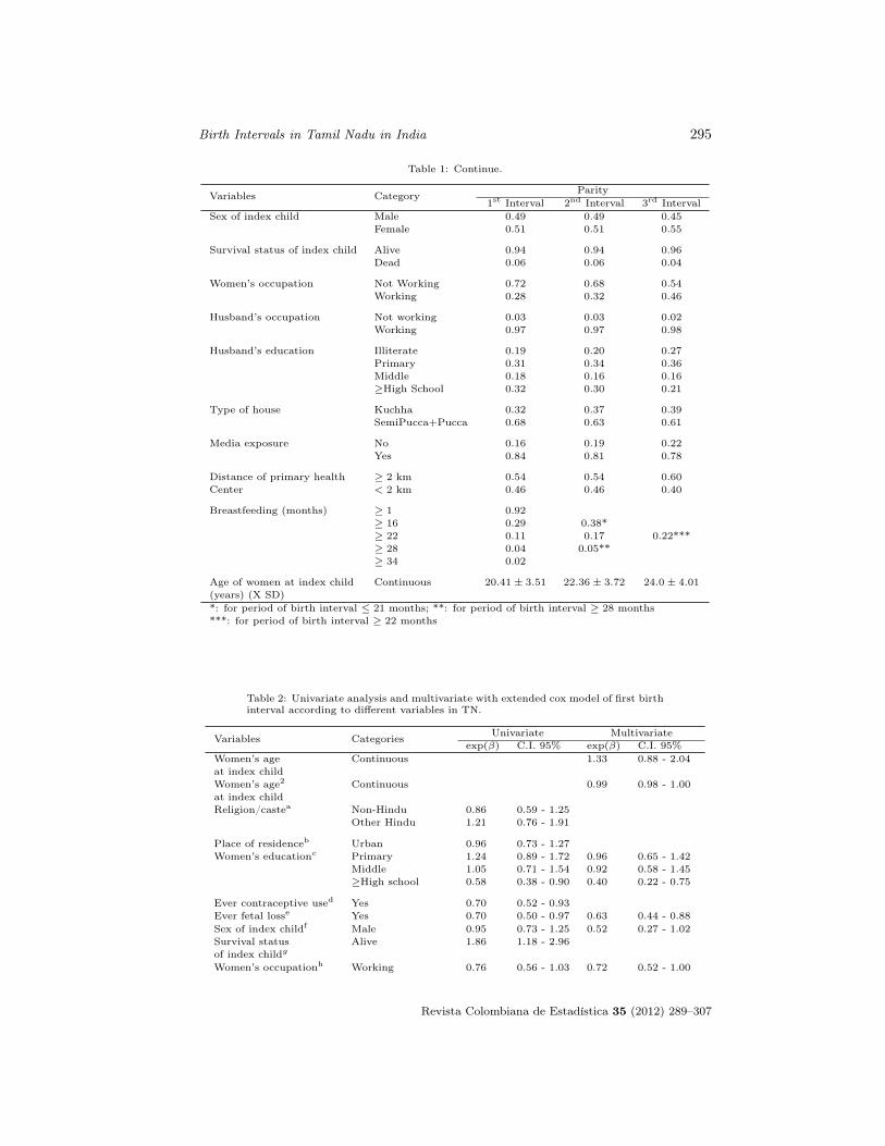
Birth Intervals in Tamil Nadu in India 295
Table 1: Continue.
Variables Category Parity1st Interval 2nd Interval 3rd Interval
Sex of index child Male 0.49 0.49 0.45Female 0.51 0.51 0.55
Survival status of index child Alive 0.94 0.94 0.96Dead 0.06 0.06 0.04
Women’s occupation Not Working 0.72 0.68 0.54Working 0.28 0.32 0.46
Husband’s occupation Not working 0.03 0.03 0.02Working 0.97 0.97 0.98
Husband’s education Illiterate 0.19 0.20 0.27Primary 0.31 0.34 0.36Middle 0.18 0.16 0.16≥High School 0.32 0.30 0.21
Type of house Kuchha 0.32 0.37 0.39SemiPucca+Pucca 0.68 0.63 0.61
Media exposure No 0.16 0.19 0.22Yes 0.84 0.81 0.78
Distance of primary health ≥ 2 km 0.54 0.54 0.60Center < 2 km 0.46 0.46 0.40
Breastfeeding (months) ≥ 1 0.92≥ 16 0.29 0.38*≥ 22 0.11 0.17 0.22***≥ 28 0.04 0.05**≥ 34 0.02
Age of women at index child Continuous 20.41 ± 3.51 22.36 ± 3.72 24.0 ± 4.01
(years) (X SD)*: for period of birth interval ≤ 21 months; **: for period of birth interval ≥ 28 months***: for period of birth interval ≥ 22 months
Table 2: Univariate analysis and multivariate with extended cox model of first birthinterval according to different variables in TN.
Variables Categories Univariate Multivariateexp(β) C.I. 95% exp(β) C.I. 95%
Women’s age Continuous 1.33 0.88 - 2.04at index childWomen’s age2 Continuous 0.99 0.98 - 1.00at index childReligion/castea Non-Hindu 0.86 0.59 - 1.25
Other Hindu 1.21 0.76 - 1.91
Place of residenceb Urban 0.96 0.73 - 1.27Women’s educationc Primary 1.24 0.89 - 1.72 0.96 0.65 - 1.42
Middle 1.05 0.71 - 1.54 0.92 0.58 - 1.45≥High school 0.58 0.38 - 0.90 0.40 0.22 - 0.75
Ever contraceptive used Yes 0.70 0.52 - 0.93Ever fetal losse Yes 0.70 0.50 - 0.97 0.63 0.44 - 0.88Sex of index childf Male 0.95 0.73 - 1.25 0.52 0.27 - 1.02Survival status Alive 1.86 1.18 - 2.96of index childg
Women’s occupationh Working 0.76 0.56 - 1.03 0.72 0.52 - 1.00
Revista Colombiana de Estadística 35 (2012) 289–307

296 Rajvir Singh, Vrijesh Tripathi, Mani Kalaivani, Kalpana Singh & S.N. Dwivedi
Table 2: Continue.
Variables Categories Univariate Multivariateexp(β) C.I. 95% exp(β) C.I. 95%
Husband’s occupationi Working 0.56 0.30 - 1.06Husband’s educationj Primary 1.05 0.73 - 1.51 1.08 0.72 - 1.61
Middle 0.86 0.56 - 1.32 0.66 0.41 - 1.08≥High school 0.70 0.48 - 1.03 0.75 0.45 - 1.26
Type of housek Pucca+Semi Pucca 0.79 0.60 - 1.04Media exposurel Yes 1.00 0.70 - 1.44Distance primary < 2 km 0.90 0.69 - 1.19health centrem
Birth interval 1-15 months 0.07 0.02 - 0.18 0.07 0.03 - 0.19Breastfeedingn ≥ 1 months 1.92 1.04 - 3.58 3.08 1.44 - 6.60Birth interval 16-21 months 0.29 0.13 - 0.62 0.30 0.14 - 0.66Breastfeedingn ≥ 16 months 0.82 0.56 - 1.19 0.74 0.50 - 1.09Birth interval 22-27 months 0.39 0.13 - 1.16 0.40 0.13 - 1.19Breastfeedingn ≥ 22 months 0.98 0.52 - 1.86 0.90 0.46 - 1.73Birth interval 28-33 months 0.46 0.04 - 4.86 0.51 0.05 - 5.51Breastfeedingn ≥ 28 months 0.54 0.14 - 2.07 0.45 0.11 - 1.74Birth interval ≥ 34 months 0.85 0.04 - 16.4 0.74 0.04 - 14.70Breastfeedingn ≥ 34 months 0.47 0.05 - 4.70 0.45 0.04 - 4.69Reference Categories: a) SC/ST Hindu, b) Rural, c) Illiterate, d) No, e) No,
f) Female, g) Dead, h) Not working, i) Not working, j) Illiterate,k) Kuccha, l) No, m) >= 2 km , n) Less than the given.
Table 3: Univariate analysis and multivariate with extended cox model of secondbirth interval according to different variables in TN.
Variables Categories Univariate Multivariateexp(β) C.I. 95% exp(β) C.I. 95%
Women’s age Continuous 0.80 0.49 - 1.29at index childWomen’s age2 Continuous 1.00 0.99 - 1.01at index childReligion/castea Non-Hindu 0.68 0.44 - 1.05
Other Hindu 0.67 0.36 - 1.26
Place of residenceb Urban 0.70 0.48 - 1.03
Women’s educationc Primary 0.72 0.47 - 1.11Middle 0.50 0.27 - 0.92≥High school 0.46 0.25 - 0.83
Ever contraceptive used Yes 0.65 0.44 - 0.97
Ever fetal losse Yes 1.00 0.67 - 1.50
Previous birth intervalf 24-36 Months 0.87 0.58 - 1.31≥ 36 Months 0.54 0.34 - 0.88
Sex of index childg Male 1.11 0.78 - 1.58
Survival status Alive 4.30 2.45 - 7.54 0.40 0.22 - 0.72of index childh
Women’s occupationi Working 1.01 0.70 - 1.47
Husband’s occupationj Working 1.22 0.38 - 3.85
Husband’s educationk Primary 0.87 0.56 - 1.37 0.72 0.46 - 1.13Middle 0.90 0.52 - 1.56 0.62 0.35 - 1.11≥High school 0.41 0.24 - 0.72 0.34 0.19 - 0.61
Revista Colombiana de Estadística 35 (2012) 289–307

Birth Intervals in Tamil Nadu in India 297
Table 3: Continue.
Variables Categories Univariate Multivariateexp(β) C.I. 95% exp(β) C.I. 95%
Type of housel Pucca+Semi Pucca 0.94 0.65 - 1.36
Media exposurem Yes 0.82 0.53 - 1.25
Distance primary < 2 km 0.68 0.47 - 0.99health centren
Birth interval 1-21 month 0.10 0.02 - 0.47 0.06 0.02 - 0.23Breastfeedingo ≥ 1 month 0.86 0.53 - 1.39 0.99 0.59 - 1.68Birth interval 22-27 month 0.07 0.01 - 0.57 0.04 0.01 - 0.57Breastfeedingo ≥ 22 month 0.99 0.47 - 2.08 1.17 0.54 - 2.52Birth interval ≥ 28 month 1.61 0.17 - 15.4 0.48 0.04 - 5.94Breastfeedingo ≥ 28 month 0.55 0.07 - 4.47 1.07 0.10 - 11.0Reference Categories: a) SC/ST Hindu, b) Rural, c) Illiterate, d) No, e) No, f) < 24 Month,
g) Female, h) Dead, i) Not working, j) Not working, k) Illiterate,l) Kuccha, m) No, n) ≥ 2 km, o) Less than the given.
Table 4: Univariate analysis and multivariate with extended cox model of thirdbirth interval according to different variables in TN.
Variables Categories Univariate Multivariateexp(β) C.I. 95% exp(β) C.I. 95%
Women’s age Continuous 0.74 0.43 - 1.26at index childWomen’s age2 Continuous 1.00 0.99 - 1.02at index childReligion/castea Non-Hindu 1.72 0.66 - 4.45
Other Hindu 1.52 0.41 - 5.66
Place of residenceb Urban 1.20 0.60 - 2.38
Women’s educationc Primary 0.76 0.33 - 1.75Middle 0.63 0.15 - 2.65≥High school 0.79 0.24 - 2.63
Ever contraceptive used Yes 0.83 0.38 - 1.81
Ever fetal losse Yes 0.50 0.22 - 1.14
Previous birth intervalf 24-36 Months 0.90 0.42 - 1.95≥ 36 Months 0.50 0.22 - 1.10
Sex of index childg Male 1.47 0.75 - 2.86
Survival status Alive 2.24 0.79 - 6.33of index childh
Women’s occupationi Working 0.81 0.42 - 1.54
Husband’s occupationj Working 0.49 0.07 - 3.61
Husband’s educationk Primary 1.45 0.62 - 3.40Middle 0.91 0.30 - 2.79≥High school 1.13 0.42 - 3.02
Type of housel Pucca+Semi Pucca 1.10 0.57 - 2.13
Media exposurem Yes 0.53 0.26 - 1.07 0.50 0.24 - 1.02
Distance primary < 2 km 0.99 0.51 - 1.92health centren
Revista Colombiana de Estadística 35 (2012) 289–307

298 Rajvir Singh, Vrijesh Tripathi, Mani Kalaivani, Kalpana Singh & S.N. Dwivedi
Table 4: Continue.
Variables Categories Univariate Multivariateexp(β) C.I. 95% exp(β) C.I. 95%
Birth interval 1-21 months 0.73 0.04 - 12.8 0.79 0.04 - 13.98
Breastfeedingo ≥ 1 months 1.73 0.23 -13.2 2.15 0.25 - 18.14
Birth interval ≥ 22 months 1.63 0.15 - 17.4 1.50 0.14 - 16.16
Breastfeedingo ≥ 22 months 0.13 0.02 - 1.00 0.13 0.05 - 1.00Reference Categories: a) SC/ST Hindu, b) Rural, c) Illiterate, d) No, e) No, f) < 24 Month,
g) Female, h) Dead, i) Not working, j) Not working, k) Illiterate,l) Kuccha, m) No, n) ≥ 2 km, o) Less than the given.
4. Multivariate Analysis
The final models consisted of varying subsets of variables for first, second, andthird birth intervals. Variables that entered partially are considered fully in thepresentation of final models for a meaningful presentation. In order to account forage which is a well-known confounder, woman’s age at index child was forced intothe model. Square of woman’s age at index child was also considered in order toovercome the problem of non-linear relationship.
The first variable to enter in the model for each birth interval was breastfeeding.Also, for each birth interval, breastfeeding alone improved the log likelihood up toa higher level, clearly showed the inclusion of breastfeeding even partially at firststep itself significantly improved the model. High improvement in chi-square withone degree of freedom was seen for each birth interval, the improvement being28.3 for first birth interval, 39.9 for second birth interval and 17.7 for third birthinterval. Surprisingly, under the first birth interval, the effect of breastfeedingpersisted only during the period 0-15 months. Also, effect of breastfeeding underthe second birth interval disappeared during each of the periods considered inthe analysis. However, its effect again persisted under the third birth intervalduring the period 22 and more months. It may be worth reporting that the roleof breastfeeding fell in line with that reported based on univariate analysis.
Before comparison of variables entered in the final extended Cox models relatedto various birth intervals, it may be noted that subsets of variables considered inthe data analysis vary from first birth interval to third birth interval because vary-ing periods of classification of breastfeeding were considered. Strictly speaking,this may prohibit a comparison among the models. However, a qualitative com-parison of results presented in Tables 2 to 4 reveals that high school (and above)education of women was a significant protective factor under the first birth intervalanalysis (HR: 0.40; C.I.: 0.22-0.75). On the other hand, high school (and above)education of father (HR: 0.34; C.I.: 0.19-0.61) and survival status of index child(HR: 0.40; C.I.: 0.22-0.72) were significant protective factors under the secondbirth interval analysis. Media exposure entered into the model for the third birthinterval. Ever-fetal loss, survival status of index child, occupation of woman andhusband’s education also entered into the model for the first birth interval. Hence,
Revista Colombiana de Estadística 35 (2012) 289–307

Birth Intervals in Tamil Nadu in India 299
variables that entered into the models varied from the first birth interval to thethird birth interval.
5. Validation of the Models
Calibration curves for extended Cox models for the birth intervals are shownin Figures 1 to 3. Except for one group with extremely bad prognosis in eachfigure, bias corrected calibrations are very good. Shrinkage coefficients related tofirst to third birth interval are 0.90, 0.92 and 0.78, respectively (Table 5). Thisclearly reveals that 10%, 8% and 22% of the model fitting will be noisy in relationto first to third birth intervals, respectively. Thus, especially in case of third birthinterval, the shrinkage coefficient could easily be used to shrink predictions to yieldbetter calibration. Table 5 also shows that the discrimination accuracy in terms ofthe calculated Somer’s Dxy rank correlation related to first to third birth intervalare −0.56, −0.62 and −0.68, respectively. This index provides good predictiveaccuracy especially in case of third birth interval. In summary, these models aregood enough to describe the parity specific birth intervals in Tamil Nadu.
Table 5: Validity indices of extended cox hazard models developed for parity specificbirth intervals.
Shrinkage Index Training Test Optimism Index ResampleCoefficient and Dxy Original Corrected
Parity-I 1.00 1.00 0.90 0.10 0.90 200−0.58 −0.59 −0.57 −0.02 −0.56 200
Parity-II 1.00 1.00 0.92 0.08 0.92 200−0.63 −0.64 −0.62 −0.01 −0.62 200
Parity-III 1.00 1.00 0.78 0.22 0.78 200−0.72 −0.74 −0.70 −0.04 −0.68 200
Dxy : Somer’s D-rank correlation.
6. Prediction from the Final Models
Prediction from the final model may be used to provide important clues topolicy planners through predicted survival probabilities at considered level of avariable by holding all other variables at their average level in the model. Inthe present prediction analysis, the possible selected variables(s) and some com-bination of variables are: women’s primary education; women’s middle educa-tion; women’s high school (and above) education; survival of index child; workingwomen; husband’s education of high school (and above); media exposure; women’shigh school (and above) education and survival index of child; and women’s highschool (and above) education and husband’s high school (and above) education.On account of varying subsets of variables in the models, only results possibleunder each model are presented in the Tables 6 to 8 that deal with first to thirdbirth intervals.
Revista Colombiana de Estadística 35 (2012) 289–307

300 Rajvir Singh, Vrijesh Tripathi, Mani Kalaivani, Kalpana Singh & S.N. Dwivedi
x
x x
x
x
x
x
x
Fra
cti
on S
urv
ivin
g 3
0 m
onth
s
Predicted 30 month Survival
1.0
0.8
0.6
0.4
0.2
0.0
0.0 0.2 0.4 0.6 0.8
Figure 1: Bootstrap estimates of calibration accuracy for 30 months estimates from thefinal extended Cox model for 1st birth interval. Dots correspond to apparentpredictive accuracy. X marks the bootstrap-corrected estimates.
x
x
x
0.8
0.6
0.4
0.2
Fra
cti
on S
urv
ivin
g 3
0 m
onth
s
0.1 0.2 0.3 0.4 0.5 0.6 0.7
Predicted 30 month Survival
Figure 2: Bootstrap estimates of calibration accuracy for 30 months estimates from thefinal extended Cox model for 2nd birth interval. Dots correspond to apparentpredictive accuracy. X marks the bootstrap-corrected estimates.
There is a decreasing trend in probability of not having next child over a periodof time related to each birth interval. This is more evident in relation to firstbirth interval. There is no specific trend with increasing period of breastfeeding.However, within each category, there is an increasing trend in not having nextchild probability in relation to increasing education of women. Women’s highschool (and above) education was noticed to provide maximum benefit. This is infurther evidence if women have a surviving index child.
Very few predictions were possible in relation to second and third birth intervals(Tables 7-8). High school (and above) education of husband provided the max-imum benefits up to the category 22-27 months under the second birth interval.Similar results were obtained in relation to survival of index child. Surprisingly,these probabilities were lower during the period of 28 and more months. Underthird birth interval, prediction was possible only in relation to media exposure.
Revista Colombiana de Estadística 35 (2012) 289–307
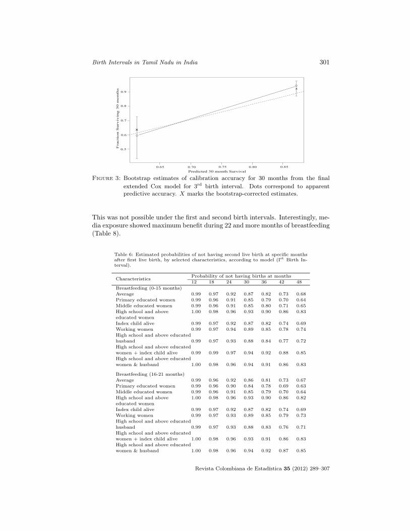
Birth Intervals in Tamil Nadu in India 301
x
x
Fra
cti
on S
urv
ivin
g 3
0 m
onth
s
0.9
0.8
0.7
0.6
0.5
Predicted 30 month Survival0.65 0.70 0.75 0.80 0.85
Figure 3: Bootstrap estimates of calibration accuracy for 30 months from the finalextended Cox model for 3rd birth interval. Dots correspond to apparentpredictive accuracy. X marks the bootstrap-corrected estimates.
This was not possible under the first and second birth intervals. Interestingly, me-dia exposure showed maximum benefit during 22 and more months of breastfeeding(Table 8).
Table 6: Estimated probabilities of not having second live birth at specific monthsafter first live birth, by selected characteristics, according to model (Ist Birth In-terval).
Characteristics Probability of not having births at months12 18 24 30 36 42 48
Breastfeeding (0-15 months)Average 0.99 0.97 0.92 0.87 0.82 0.73 0.68Primary educated women 0.99 0.96 0.91 0.85 0.79 0.70 0.64Middle educated women 0.99 0.96 0.91 0.85 0.80 0.71 0.65High school and above 1.00 0.98 0.96 0.93 0.90 0.86 0.83educated womenIndex child alive 0.99 0.97 0.92 0.87 0.82 0.74 0.69Working women 0.99 0.97 0.94 0.89 0.85 0.78 0.74High school and above educatedhusband 0.99 0.97 0.93 0.88 0.84 0.77 0.72High school and above educatedwomen + index child alive 0.99 0.99 0.97 0.94 0.92 0.88 0.85High school and above educatedwomen & husband 1.00 0.98 0.96 0.94 0.91 0.86 0.83
Breastfeeding (16-21 months)Average 0.99 0.96 0.92 0.86 0.81 0.73 0.67Primary educated women 0.99 0.96 0.90 0.84 0.78 0.69 0.63Middle educated women 0.99 0.96 0.91 0.85 0.79 0.70 0.64High school and above 1.00 0.98 0.96 0.93 0.90 0.86 0.82educated womenIndex child alive 0.99 0.97 0.92 0.87 0.82 0.74 0.69Working women 0.99 0.97 0.93 0.89 0.85 0.79 0.73High school and above educatedhusband 0.99 0.97 0.93 0.88 0.83 0.76 0.71High school and above educatedwomen + index child alive 1.00 0.98 0.96 0.93 0.91 0.86 0.83High school and above educatedwomen & husband 1.00 0.98 0.96 0.94 0.92 0.87 0.85
Revista Colombiana de Estadística 35 (2012) 289–307

302 Rajvir Singh, Vrijesh Tripathi, Mani Kalaivani, Kalpana Singh & S.N. Dwivedi
Table 6: Continue.
Characteristics Probability of not having births at months12 18 24 30 36 42 48
Breastfeeding (22-27 months)Average 0.99 0.96 0.87 0.79 0.72 0.61 0.67Primary educated women 0.98 0.94 0.85 0.76 0.68 0.56 0.48Middle educated women 0.98 0.94 0.86 0.77 0.69 0.57 0.50High school and above 1.00 0.97 0.94 0.90 0.85 0.79 0.83educated womenindex child alive 0.99 0.95 0.88 0.80 0.73 0.62 0.55Working women 0.99 0.96 0.90 0.83 0.77 0.67 0.61High school and above educatedhusband 0.99 0.95 0.89 0.82 0.75 0.65 0.58High school and above educatedwomen + index child alive 0.99 0.97 0.94 0.90 0.86 0.79 0.75High school and above educatedwomen & husband 0.99 0.98 0.94 0.91 0.87 0.81 0.77
Breastfeeding (28-33 months)Average 0.99 0.96 0.92 0.86 0.81 0.73 0.67Primary educated women 0.99 0.96 0.90 0.84 0.78 0.69 0.63Middle educated women 0.99 0.96 0.91 0.85 0.79 0.70 0.64High school and above 1.00 0.98 0.96 0.93 0.90 0.86 0.83educated womenIndex child alive 0.99 0.97 0.92 0.87 0.82 0.73 0.68Working women 0.99 0.97 0.93 0.89 0.85 0.78 0.73High school and above educatedhusband 0.99 0.97 0.93 0.88 0.83 0.76 0.71High school and above educatedwomen + index child alive 1.00 0.98 0.96 0.94 0.91 0.87 0.84High school and above educatedwomen & husband 1.00 0.98 0.96 0.93 0.90 0.86 0.83
Breastfeeding (≥ 34 months)Average 0.99 0.95 0.88 0.81 0.73 0.63 0.56Primary educated women 0.98 0.94 0.86 0.78 0.70 0.58 0.51Middle educated women 0.99 0.94 0.87 0.79 0.71 0.59 0.52High school educated women 0.99 0.97 0.94 0.90 0.86 0.80 0.76Index child alive 0.99 0.95 0.89 0.81 0.74 0.64 0.57Working women 0.99 0.96 0.90 0.84 0.78 0.69 0.63High school and above educatedhusband 0.99 0.96 0.90 0.73 0.77 0.67 0.61High school and above educatedwomen + index child alive 0.99 0.98 0.94 0.90 0.86 0.80 0.76High school and above educatedwomen & husband 0.99 0.98 0.94 0.90 0.86 0.80 0.76
Revista Colombiana de Estadística 35 (2012) 289–307

Birth Intervals in Tamil Nadu in India 303
Table 7: Estimated probabilities of not having third live birth at specific months aftersecond live birth in TN, by selected characteristics, according to model (IInd
Birth Spacing).
Characteristics Probability of not having births at months12 18 24 30 36 42 48
Breastfeeding (16-21 months)Average 1.00 1.00 0.99 0.98 0.98 0.97 0.95High school and above 1.00 1.00 0.99 0.99 0.99 0.98 0.97educated womenIndex child alive 1.00 1.00 0.99 0.98 0.98 0.97 0.95
Breastfeeding(22-27 months)Average 1.00 1.00 1.00 0.99 0.99 0.99 0.98High school and above husband 1.00 1.00 1.00 1.00 1.00 0.99 0.99Index child alive 1.00 1.00 1.00 0.99 0.99 0.99 0.98
Breastfeeding (≥ 28 months)Average 0.99 0.91 0.79 0.68 0.62 0.50 0.33High school and above husband 0.99 0.95 0.87 0.80 0.76 0.68 0.53Index child alive 0.99 0.91 0.80 0.69 0.63 0.52 0.35
Table 8: Estimated probabilities of not having fourth live birth at specific months afterthird live birth in TN, by selected characteristics, according to model (IIIrd
Birth Spacing).
Characteristics Probability of not having births at months12 18 24 30 36 42 48
Breastfeeding (0-21 months)Average 0.99 0.95 0.90 0.83 0.78 0.71 0.71Media exposure 0.99 0.96 0.91 0.85 0.81 0.75 0.75
Breastfeeding (≥ 22 months)Average 1.00 0.99 0.97 0.95 0.94 0.91 0.91Media exposure 1.00 0.99 0.98 0.96 0.95 0.93 0.93
7. Discussion
To our knowledge, there is no study on birth interval, in which an exerciserelated to the validity of the developed Cox hazards models has been carried out.Therefore, there is no scope to compare the developed models in the present studywith those reported under other studies, especially with regard to validity of themodels. However, if necessary, one could examine the reported likelihood valuesfor models under other studies to provide for a comparison with models developedin the present study.
Breastfeeding is the only covariate, which is noticed to be a significant pro-tective factor associated with each birth interval. Education of women was sig-nificantly associated with first birth interval only while husband’s education wassignificantly associated with first and second birth interval. Survival status of in-dex child emerged as an important associated factor at second birth interval onlywhile fetal loss was associated at the first birth interval. However, contraceptiveuse did not emerge as a significant associated factor at any birth interval.
Revista Colombiana de Estadística 35 (2012) 289–307

304 Rajvir Singh, Vrijesh Tripathi, Mani Kalaivani, Kalpana Singh & S.N. Dwivedi
Breastfeeding is the most important and significant factor for extending thebirth interval at all the parities in TN. Trussell et al. (1985) in a study done in thePhilippines, Malaysia, and Indonesia also found breastfeeding beyond 11 monthsto be a significant protective factor on birth interval. Anderson & Bean (1985)also support the relation between ever breastfeeding and exclusive breastfeedingand birth interval. Thus, though the relation between breastfeeding and birthinterval is already documented, this study is able to predict the precise nature ofthis effect.
Education of woman high school (and above) was a protective factor for the firstbirth interval. This finding is supported by Rajaram, Rao & Pandey (1994) andGandotra, Retherford, Pandey, Luther & Mishra (1998), who found that educationof woman led to reduction in fertility, probably due to increase in awareness andchoice. In contrast, Rodriguez, Hobcraft, McDonald, Menken & Trussell (1984)found little association between education and birth interval except at higher par-ities. Ojha (1998) and Richter, Podhisita, Chamratrithirong & Soonthorndhada(1994) support Rodriguez’s findings. A similar reasoning can be attributed to thefact that media exposure had a protective impact on higher order birth interval.This finding is supported by Gandotra et al. (1998).
This study has clearly indicated that working status of women was a significantprotective factor specifically for the first birth interval in TN. While this is notsupported by Trussell et al. (1985), Richter et al. (1994) noticed that womenemployed as salesgirls and manufacturing laborer and in self-employment weresignificantly less likely to go for the next birth.
Ojha (1998) and Blanchard & Bogaert (1997) reported that birth intervals arecomparatively longer following the birth of a male in comparison to female child.However, sex of index child did not emerge as a significant associated factor. Thepresent study did not indicate the likelihood of it being a protective factor at anybirth interval.
Survival of index child emerged as a significant protective factor for the firstand second birth intervals. This was in line with many other studies like Oheneba-Sakyi & Heaton (1993); Rehman & DaVanzo (1993) Rajaram et al. (1994); Ojha(1998); and Palloni & Hantamala (1999). This shows that this factor is not acountry or region specific determinant.
Other documented factors such as contraceptive use (Rajaram et al. 1994, Mah-mud & Islam 1995), place of residence (Swenson & Thang 1993) and importanceof previous birth interval in extending succeeding birth intervals (Rodriguez et al.1984, DaVanzo & Starbird 1991, Miller, Trussell, Pabley & Vaughan 1992, Swenson& Thang 1993, Trussell et al. 1985) were not supported in this study.
8. Limitations
First National Health and Family Survey (NFHS) was conducted in 1992-93in India and data was available to use in 1995. However, no study is available tillnow on breastfeeding as a time varying covariate with time dependent effect using
Revista Colombiana de Estadística 35 (2012) 289–307

Birth Intervals in Tamil Nadu in India 305
bootstrap technique for validations and predictions. These techniques have beenused for the first time on birth interval data. Our internet search has not revealedany similar study. Therefore, we felt that the study has valuable information forstrategic and policy planners and gives more occasion for readership.
9. Conclusion
This study showed that subsets of important covariates, which entered intothe final models, varied among the birth intervals within the state. However, theassessment of predictive accuracy clearly established the suitability of the parityspecific developed models in describing respective birth interval. Thus, the presentstudy emphasizes the need for regional studies in planning public health programsas per needs of the region. Further, this study also demonstrates the importanceof parity specific analysis of birth interval and may assist in working out parityspecific strategies in the considered region. Breastfeeding emerged as an importantprotective covariate that extended the birth interval irrespective of parity. Further,education of women, sex of index child, husband’s education, and media exposurealso demonstrated an important protective role for extending birth interval in thestudy.
[Recibido: agosto de 2011 — Aceptado: marzo de 2012]
References
Anderson, D. L. & Bean, L. L. (1985), ‘Birth spacing and fertility limitation: Abehavioral analysis of nineteenth century populationl’, Demography 22, 169–183.
Blanchard, R. & Bogaert, A. F. (1997), ‘Additive effects of older brothers and ho-mosexual brothers in the prediction of marriage and cohabitation’, BehaviorGenetics 27, 45–54.
Cox, D. R. (1972), ‘Regression models and life tables (with Discussion)’, Journalof the Royal Statistical Society, Series B 34, 187–220.
DaVanzo, J. & Starbird, E. (1991), ‘Correlates of short interbirth intervals inpeninsular Malaysia: Their pathways of influence through breastfeeding andcontraceptive use’, Studies in Family Planning 22(4).
Dickson, E., Grambsch, P., Fleming, T., Fisher, L. & Langworthy, A. (1989),‘Prognosis in primary biliary cirrohsis: Model for decision making’, Hepatol-ogy 10(1), 1–7.
Dwivedi, S. & Rajvir, S. (2003), ‘On assessing the child spacing effect of breast-feeding using cox proportional hazards model with nfhs data’, DemographyIndia 32(2), 215–224.
Revista Colombiana de Estadística 35 (2012) 289–307

306 Rajvir Singh, Vrijesh Tripathi, Mani Kalaivani, Kalpana Singh & S.N. Dwivedi
Efron, B. & Tibshirani, R. (1993), An Introduction to the Bootstrap, Chapmanand Hall, New York.
Fox, J. (2008), Applied Regression Analysis, Linear Models, and Related Methods,Sage Publications, Inc., London.
Gandotra, M., Retherford, R., Pandey, A., Luther, N. & Mishra, V. (1998), Fer-tility in India, National Family Health Survey Subject Reports 9, Mumbai:International Institute for Population Sciences; and Honolulu.
Harrell, F. E. (2001), Regression Modeling Strategies with Application to LinearModels, Logistic Regression, and Survival Analysis, Springer-Verlag, Berlin.
Harrell, F. E., Lee, K. L. & Mark, D. B. (1996), ‘Tutorial in Biostatistics Multivari-able prognostic models: Issues in developing models, evaluating assumptionsand adequacy, and meassuring and reducing errors’, Statistics in Medicine15, 361–387.
International Institute for Population Sciences (1994), National Family HealthSurvey (MCH and Family Planning), Tamil Nadu 1992, Summary report,Population Research Centre, The Gandhigram Institute of Rural Health andFamily Welfare Trust, Ambathurai R.S. (PRC, Gandhigram), and Interna-tional Institute for Population Sciences (IIPS), Bombay, India.
International Institute for Population Sciences (1995), National Family HealthSurvey (MCH and Family Planning): India 1992-93, Summary report, Inter-national Institute for Population Sciences (IIPS), Bombay, India.
Kaplan, E. & Meier, P. (1958), ‘ Nonparametric estimation from incomplete ob-servations’, Journal of the American Statistical Association 53, 457–481.
Kleinbaum, D. G. (1996), Survival Analysis, A Self Learning Text, 1 edn, Springer-Verlag, New York.
Mahmud, M. & Islam, M. (1995), ‘Adolescent contraceptive use and its deter-minants in Bangladesh: Evidence from Bangladesh Fertility Survey 1989.’,Contraception 52(3), 181–186.
Miller, J. E., Trussell, J., Pabley, A. R. & Vaughan, B. (1992), ‘Birth spacing andchild mortality in Bangladesh and the Philippines’, Demography 29(2), 305–316.
Namboodiri, K. & Suchindran, C. M. (1987), Life Table Techniques and TheirApplications Studies in Population, Academic Press, Orlando, Florida.
Oheneba-Sakyi, Y. & Heaton, T. B. (1993), ‘Effects of socio-demographic vari-ables on birth intervals in Ghana’, Journal of Comparative Family Studies24(1), 113–135.
Ojha, A. (1998), ‘The effect of sex preference on fertility in selected states of India’,The Journal of Family Welfare 44(1), 42–48.
Revista Colombiana de Estadística 35 (2012) 289–307

Birth Intervals in Tamil Nadu in India 307
Palloni, A. & Hantamala, R. (1999), ‘The effects of infant mortality on fertilityrevisited: New evidence from Latin America’, Demography 36(1), 41–75.
Rajaram, S., Rao, S. & Pandey, A. (1994), ‘Birth interval dynamics in Goa: Aparity specific analysis’, Demography India 23(1), 67–81.
Rehman, M. & DaVanzo, J. (1993), ‘ Gender preference and birth spacing inMatlab, Bangladesh’, Demography 30(3), 315–332.
Richter, K., Podhisita, C., Chamratrithirong, A. & Soonthorndhada, K. (1994),‘The impact of child care on fertility in urban Thailand’, Demography31(4), 651–662.
Rodriguez, G., Hobcraft, J., McDonald, J., Menken, J. & Trussell, J. A. (1984),‘Comparative analysis of the determinants of birth intervals’, WFS Compar-ative Studies (30).
Singh, R., Begum, S., Ahuja, R. K., Chandra, P. & Dwivedi, S. N. (2007), ‘Pre-diction of child survival in India using developed Cox PH model: a utility forhealth policy programmers’, Statistics in Transition 8(1), 97–110.
Srinivasan, K. (1980), Birth interval analysis in fertility surveys, in ‘World FertilitySurvey Scientific Reports’, number 7:19, Voorburg and London.
Swenson, I. & Thang, N. M. (1993), ‘Determinants of birth intervals in Vietnam:A hazard model analysis’, Journal of Tropical pediatrics 39, 163–167.
Trussell, J. & Charles, H. (1983), ‘A hazards model analysis of the covariates ofinfant and child mortality in Sri Lanka’, Demography 20(1), 1–24.
Trussell, J., Martin, L., Fledman, R., Palmore, J., Concepcion, M. & Abu Bakar,D. (1985), ‘Determinants of birth interval length in the Phillipines, Malaysiaand Indonesia: A hazard model analysis’, Demography 22(2).
UNFPA (1997), Reproductive Rights, Reproductive Health and Family Planning,Population issues, United Nations Fund for Population Activities (UNFPA).
Van Houwelingen, J. C. & Cessie, S. (1990), ‘Predictive value of statistical models’,Statistics in Medicine 8, 1303–1325.
Revista Colombiana de Estadística 35 (2012) 289–307


Revista Colombiana de EstadísticaNúmero especial en Bioestadística
Junio 2012, volumen 35, no. 2, pp. 309 a 330
Random Regression Models for Estimation ofCovariance Functions, Genetic Parameters and
Prediction of Breeding Values for Rib Eye Area ina Colombian Bos indicus-Bos taurus Multibreed
Cattle Population
Modelos de regresión aleatoria para la estimación de funciones decovarianza, parámetros genéticos y predicción de valores genéticos en
una población bovina multirracial Bos indicus-Bos taurus enColombia
Carlos Alberto Martínez1,2,a, Mauricio Elzo2,b, Carlos Manrique1,c,Luis Fernando Grajales4,d, Ariel Jiménez1,3,e
1Grupo de Estudio en Mejoramiento y Modelación Animal GEMA, Departamentode Producción Animal, Universidad Nacional de Colombia, Bogotá, Colombia2Department Animal Sciences, University of Florida, Florida, United States3Asociación Colombiana de Criadores de Ganado Cebu ASOCEBU, Bogota,
Colombia4Departamento de Estadística, Facultad de Ciencias, Universidad Nacional de
Colombia, Bogota, Colombia
Abstract
In this paper we present an application of random regression models(RRM) to obtain restricted maximum likelihood estimates of covariancefunctions and predictions of breeding values for longitudinal records of ribeye area measured by ultrasound (REA) in a Colombian multibreed cattlepopulation. The dataset contained 708 records from 340 calves progeny of 37sires from nine breeds mated to Gray Brahman Cows. The mixed model wasa RRM that used Legendre polynomials (LP) of order 1 to 3. Fixed effectswere age of animal, dam parity, contemporary group (herd*year*season*sex),breed additive genetic and heterosis, whereas direct and maternal additivegenetic and maternal permanent environment were random effects. Residual
aMSc in Quantitative Genetics. E-mail: [email protected]. E-mail: [email protected]. E-mail: [email protected] professor. E-mail: [email protected] in Quantitative Genetics. E-mail: [email protected]
309

310 Carlos Alberto Martínez, et al.
variances were modeled either as constant or changing across the growth tra-jectory. Models were compared with two Information Criteria, the correctedAkaike’s and the Schwartz’s Bayesian. According to these criteria the bestmodel was the one with first order LP and constant residual variance. Giventhat with this model estimated maternal additive genetic and permanentenvironment covariance functions showed that these effects were not accu-rately disentangled, a parsimonious model without maternal additive geneticeffects was used to obtain genetic parameters and breeding values. Directadditive genetic variance decreased until 150 days and then increased. Mater-nal permanent environment variance increased with age. Direct heritabilityestimates for REA at 4 months, weaning, 12 and 15 months (considered astarget ages), were 0.003, 0.007, 0.034 and 0.058, respectively. Direct addi-tive correlations ranged from −0.7 to 1. Maternal permanent environmentalcorrelations were close to unity across the entire range of ages. Estimatesof (co)variance components showed the need to validate results with largermultigenerational multibreed populations before implement RRM in regionalor national genetic evaluation procedures in Colombia.
Key words: Animal population, Covariance functions, Mixed model.
Resumen
En este trabajo presentamos una aplicación de modelos de regresiónaleatoria (RRM) para obtener estimadores de máxima verosimilitud restrin-gida de funciones de covarianza y predicciones del valor genético para datoslongitudinales de área de ojo del lomo medidos por ultrasonido (REA) en unapoblación bovina multirracial en Colombia. El conjunto de datos contenía708 registros de 340 animales descendientes de 37 toros de 9 razas apareadoscon hembras Brahman Gris. Los modelos mixtos empleados fueron RRM queusaron polinomios de Legendre (LP) de orden 1 a 3. Los efectos fijos fueronedad del animal, número de partos de la madre, grupo contemporáneo (ha-cienda*año*época*sexo), efectos genéticos aditivos de raza y heterosis, mien-tras que los efectos genéticos aditivos directos y maternos y de ambiente per-manente materno fueron aleatorios. Las varianzas residuales se modelaroncomo constantes o cambiantes a través de la trayectoria de crecimiento. Losmodelos fueron comparados mediante el criterio de información de Akaikecorregido y el de información bayesiana de Schwartz. Según esos criterios,el mejor modelo fue aquel con LP de orden 1 y varianza residual constante.Dado que con este modelo las estimaciones de las funciones de covarianzagenética aditiva materna y de ambiente permanente materno indicaron queestos dos efectos no se separaron adecuadamente, un modelo más parsimo-nioso sin los efectos genéticos aditivos maternos fue empleado para obtenerparámetros y valores genéticos. La varianza genética aditiva directa decre-ció hasta 150 días y luego aumentó. La varianza de ambiente permanentematerno aumentó con la edad. Las estimaciones de heredabilidad directapara REA a los 4 meses, destete, 12 y 15 meses (consideradas como edades dereferencia) fueron 0.003, 0.007, 0.034 y 0.058, respectivamente. Las correla-ciones aditivas directas variaron de −0.7 a 1. Las correlaciones de ambientepermanente materno fueron cercanas a la unidad a través de todo el rangode edades. Las estimaciones de componentes de (co)varianza mostraron la
Revista Colombiana de Estadística 35 (2012) 309–330

Random regression models for genetic longitudinal data 311
necesidad de validar los resultados con poblaciones multirraciales multigen-eracionales mayores antes de implementar RRM en procedimientos de eval-uación genética regionales o nacionales en Colombia.
Palabras clave: modelo mixto, funciones de covarianza, población animal.
1. Introduction
Modeling of longitudinal records with Legendre polynomials (LP) was proposedby Kirkpatrick, Lofsvold & Bulmer (1990) to describe direct additive genetic co-variances among records at any pair of ages in a continuous form. The LP aresolutions to the Legendre’s differential equation and they are orthogonal. Thisproperty allows describing patterns of genetic variation through a growth tra-jectory. Continuous functions representing covariances among records are calledcovariance functions (Kirkpatrick et al. 1990). Meyer (1998) suggested that coef-ficients of covariance functions could be estimated as covariances among randomregression coefficients by fitting linear mixed models. Advantages of random re-gression over multiple trait models (MTM) involve the inclusion of all availabledata without pre-adjustment to particular ages, no lose of records taken outsidecertain age ranges, and reduction in the number of parameters to be estimated byfitting parsimonious models (Kirkpatrick et al. 1990, Meyer & Hill 1997). Untiltoday, these models have not been implemented for genetic analysis in Colombia.Carcass quality is important in the current beef market. Thus, there exists greatinterest in carcass traits measured by ultrasound like the rib eye area (REA), be-cause they are closely related to the true carcass values and meat yields (Hougton& Turlington 1992). Genetic evaluation of carcass traits has been implemented inanimal breeding programs in different countries and species (Wilson 1992, Hassen,Wilson & Rouse 2003, Fischer, van der Werf, Banks, Ball & Gilmour 2006, Choy,Lee, Kim, Choi, Choi & Hwang 2008). However, few genetic studies have con-sidered ultrasound carcass traits in a longitudinal manner either in purebred orcrossbred cattle (Fischer et al. 2006, Speidel, Enns, Brigham & Keeman 2007, Mer-cadante, El Faro, Pinheiro, Cyrillo, Bonilha & Branco 2010). Jiménez, Manrique& Martínez (2010) conducted the only study in Colombia on ultrasound carcasstraits in cattle under pasture conditions using purebred Brahman. In low trop-ical areas of Colombia, there are limiting environmental conditions for livestockproduction. Consequently, crossbreeding between native Creole or European (Bostaurus) with Zebu (Bos indicus) breeds is frequently used as a strategy to in-crease beef production while maintaining adaptability (FEDEGAN 2006). Thismating strategy has created a need to establish genetic evaluation programs in-volving animals from temperate and tropically adapted breeds for carcass traits.These programs must take into consideration that 72% of the Colombia’s cattlepopulation is Zebu (mainly Brahman) (FEDEGAN 2006). Thus, the objective ofthis research was to show how to apply the RRM to obtain restricted maximumlikelihood estimates of covariance functions and predictions of breeding values forlongitudinal records of rib eye area measured by ultrasound (REA) in a Colombianmultibreed cattle population.
Revista Colombiana de Estadística 35 (2012) 309–330
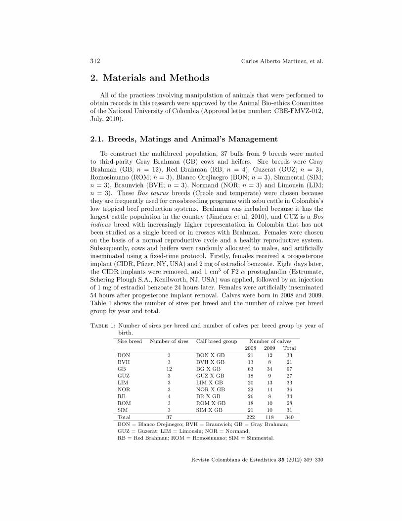
312 Carlos Alberto Martínez, et al.
2. Materials and Methods
All of the practices involving manipulation of animals that were performed toobtain records in this research were approved by the Animal Bio-ethics Committeeof the National University of Colombia (Approval letter number: CBE-FMVZ-012,July, 2010).
2.1. Breeds, Matings and Animal’s Management
To construct the multibreed population, 37 bulls from 9 breeds were matedto third-parity Gray Brahman (GB) cows and heifers. Sire breeds were GrayBrahman (GB; n = 12), Red Brahman (RB; n = 4), Guzerat (GUZ; n = 3),Romosinuano (ROM; n = 3), Blanco Orejinegro (BON; n = 3), Simmental (SIM;n = 3), Braunvieh (BVH; n = 3), Normand (NOR; n = 3) and Limousin (LIM;n = 3). These Bos taurus breeds (Creole and temperate) were chosen becausethey are frequently used for crossbreeding programs with zebu cattle in Colombia’slow tropical beef production systems. Brahman was included because it has thelargest cattle population in the country (Jiménez et al. 2010), and GUZ is a Bosindicus breed with increasingly higher representation in Colombia that has notbeen studied as a single breed or in crosses with Brahman. Females were chosenon the basis of a normal reproductive cycle and a healthy reproductive system.Subsequently, cows and heifers were randomly allocated to males, and artificiallyinseminated using a fixed-time protocol. Firstly, females received a progesteroneimplant (CIDR, Pfizer, NY, USA) and 2 mg of estradiol benzoate. Eight days later,the CIDR implants were removed, and 1 cm3 of F2 α prostaglandin (Estrumate,Schering Plough S.A., Kenilworth, NJ, USA) was applied, followed by an injectionof 1 mg of estradiol benzoate 24 hours later. Females were artificially inseminated54 hours after progesterone implant removal. Calves were born in 2008 and 2009.Table 1 shows the number of sires per breed and the number of calves per breedgroup by year and total.
Table 1: Number of sires per breed and number of calves per breed group by year ofbirth.Sire breed Number of sires Calf breed group Number of calves
2008 2009 TotalBON 3 BON X GB 21 12 33BVH 3 BVH X GB 13 8 21GB 12 BG X GB 63 34 97GUZ 3 GUZ X GB 18 9 27LIM 3 LIM X GB 20 13 33NOR 3 NOR X GB 22 14 36RB 4 BR X GB 26 8 34ROM 3 ROM X GB 18 10 28SIM 3 SIM X GB 21 10 31Total 37 222 118 340BON = Blanco Orejinegro; BVH = Braunvieh; GB = Gray Brahman;GUZ = Guzerat; LIM = Limousin; NOR = Normand;RB = Red Brahman; ROM = Romosinuano; SIM = Simmental.
Revista Colombiana de Estadística 35 (2012) 309–330

Random regression models for genetic longitudinal data 313
Animals were kept in two herds located in Southern Cesar, municipality ofAguachica, Colombia. The ecosystem in this micro region is a very dry tropicalforest. This region has a mean annual temperature of 28 , a height above sea levelof 50 m, a relative humidity of 80% and sandy-loam soils. Because of its environ-mental conditions, Southern Cesar is considered to be better suited for beef cattleproduction than other regions in Colombia. The feeding system was based on pas-tures. Grass species were Brachipará (Brachiaria plantaginea), Guinea (Panicummáximum) and Angleton (Dichantium aristatum). Pastures were not fertilized.Animals were provided with an 8% phosphorus mineral supplement (GANASAL®,Colombia). Mineral supplement consumption was ad libitum. The grazing systemwas rotational with a rotation period of 60 days. All calves were weaned between7 and 8 months of age and males were castrated at 12 months of age.
2.2. Records
The REA records were taken by a certified technician of the Colombian ZebuCattle Breeders Association (ASOCEBU, Bogotá D.C., Colombia) using an AquilaEsaote model device (Pie Medical Equipment B.V., Maastricht, Limburg, TheNetherlands). Once ultrasound images were collected, they were analyzed to checkquality and to obtain the REA values (cm2) using the Echo Image Viewer softwareof Pie Medical (Pie Medical Equipment B.V., Maastricht, Limburg, The Nether-lands). The total number of REA records was 708. Age of animals ranged from70 to 492 days. Records were intended to be taken approximately at four, eight(weaning), twelve and fifteen months. Mean ages at each of these data collectionpoints were: 120, 233, 332 and 445 days. At 4 months of age, calves are moredependent on the cow’s milk production that at weaning. This is due to the factthat at this stage the calf has not finished its transition from pre-ruminant to ru-minant (Van Soest 1994). Thus, REA measurements taken at this age are usefulto evaluate maternal effects (both genetic and non genetic).
2.3. Genetic Analysis
Mixed models procedures were carried out to obtain restricted maximum likeli-hood (REML) estimates of covariance components and best linear unbiased predic-tors (BLUP) of animal breeding values (BV). The following effects were assumedto be fixed in the mixed model: Contemporary group (herd*year*season*sex sub-class), breed group additive effects, non additive effects (individual heterosis), damparity (heifer or third parity cow) and age of the animal (linear and quadraticeffects). In a first approach, the random effects were: Direct additive genetic, ma-ternal additive genetic, maternal permanent environment, and residual. Seasonswithin years were defined as rainy or dry. The first season was a rainy season frommid April to mid August of 2009, the second was a dry season from mid August tomid December of 2009, the third was a dry season from mid December of 2009 tomid April of 2010, and the fourth was a rainy season from mid April to mid Augustof 2010. The GB and RB bulls were grouped as a single breed (BR). Thus, therewere 8 breed groups for calves: BR x GB, BON X GB, BVH X GB, GUZ X GB,
Revista Colombiana de Estadística 35 (2012) 309–330

314 Carlos Alberto Martínez, et al.
LIM X GB, NOR X GB, ROM X GB and SIM X GB. Breed group effects weremodeled as a continuous function of breeds over time. This function was a linearLP. Additive genetic breed group effects were modeled in such a way because indi-vidual random deviations and breed group solutions are required to obtain BV ata particular age in a multibreed population (Elzo & Wakeman 1998). In addition,because of the orthogonality of LP, the block of the mixed model equations corre-sponding to breed group effects was an identity matrix, thus, multicollinearity andconfounding problems that are commonly present among genetic fixed effects inmultibreed populations (Elzo & Famula 1985) could be alleviated at least partially.To estimate covariance functions (CF) for the following effects: Direct additivegenetic (DAGCF), maternal additive genetic (MAGCF) and maternal permanentenvironment (MPECF) and to compute BV, the regression variables used werenormalized LP (LP with norm 1), evaluated at age of animal when records werecollected. Orders of LP ranged from 1 to 3. The following combinations of LP todescribe direct additive, maternal additive and maternal permanent environmentCF were used: one (LP1), 2(LP2) and 3(LP3) for the 3 covariance components,and 3 for direct additive genetic covariances and 2 for maternal additive geneticand permanent environment covariances (LP32). The orders of LP were definedtaking into account data set size and literature reports (Fischer et al. 2006, Mer-cadante et al. 2010). The residual variance was modeled in two ways. The first oneassumed that the residual variance was the same along the entire growth trajec-tory (LP1HOM, LP2HOM, LP3HOM, LP32HOM), and the second one assumeda step function (LP1HET, LP2HET, LP3HET, LP32HET) across 3 age intervals(70 ≤ age ≤ 230 days, 230 < age ≤ 365 days, and 365 < age ≤ 492 days). Resid-uals were assumed to be independent and normally distributed. Thus, there werea total of 8 random regression models to compare: LP1HET, LP2HET, LP3HET,LP32HET, LP1HOM, LP2HOM, LP3HOM, and LP32HOM. Models comparisonwas made through the Schwartz’s Bayesian Information Criterion (BIC) and theCorrected Akaike’s Information Criterion (AICC):
BIC = −2 logL+K log(N − r)
AICC = AIC +(2(K + 1)(K + 2))
(N −K − 2)
Where AIC is the Akaike’s information criterion, K is the number of param-eters, N is the number of records, logL is the natural logarithm of the likelihoodfunction and r is the rank of the fixed part of the model, that is, the rank of theincidence matrix for all fixed effects in the model. The AICC was preferred overthe AIC in our study because of the small data set size, which is suggested byLittell, Milliken, Stroup, Wolfinger & Schabenberger (2006). However, estimatedcovariance functions showed a strong negative correlation among maternal addi-tive genetic and maternal environmental effects, which indicated that these effectswere not accurately separated. Thus, a parsimonious version of the model selectedin the first approach (LP1HOM) considering only maternal permanent environ-mental effects and denoted as LP1HOMS was used to compute variance-covariancecomponents, genetic parameters and BV. The number of variance-covariance pa-rameters ranged from 7 for the most parsimonious model (LP1HOMS) to 33 for
Revista Colombiana de Estadística 35 (2012) 309–330

Random regression models for genetic longitudinal data 315
model LP4HET (Table 2). In matrix notation the RRM used was as follows:
y = Xβ +Qgaga +Qhh+ Φaa+ Φpp+ e
V ar
ape
=
A⊗Ka
I ⊗Kp
R
E[y] = Xβ +Qgaga +Qhh
V ar(y) = Φa(A⊗Ka)Φ′a + Φp(I ⊗Kp)Φ′p +R
Table 2: Akaike’s corrected information criterion (AICC), Schwartz’s Bayesian infor-mation criterion (BIC), residual analysis and number of parameters for eachmodel.
Model AICC BIC Number of variance covariance parameters Log L1
LP1HET 3394.74 3448.66 12 −1685.15LP2HET 3412.64 3506.42 21 −1684.65LP3HET 3435.54 3581.68 33 −1683.10LP32HET 3426.62 3555.42 29 −1683.03LP1HOM 3392.82 3437.8 10 −1686.25LP2HOM 3410.66 3495.62 19 −1685.78LP3HOM 3508.34 3645.82 31 −1721.70LP32HOM 3426.66 3546.72 27 −1685.22LP1HOMS 3386.66 3418.21 7 −1686.251Natural logarithm of the restricted likelihood function.
Where y = vector containing the REA records, β = vector of unknown fixedeffects of contemporary group, dam parity and age of animal, ga = vector offixed additive genetic group effects (modeled as a continuous function of time)which correspond to the mean effects of genes from a given breed (Elzo 2010),h = vector of fixed non additive genetic effects (individual heterosis) these arethe effects due to the presence of alleles from different breeds in one locus (Elzo2010), a = vector of random regression coefficients for direct additive geneticeffects, which are the sum of effects of individual genes affecting REA (Kempthorne1957, Lynch & Walsh 1998), p = vector containing random regression coefficientsfor maternal permanent environmental effects, which correspond to those effectsexplained by the environment proportioned to the calf by its dam, maternal effectsare genetic to the dam and environmental to the calf, e = random vector ofresiduals, X, Qga, Qh, Φa, Φp were known incidence matrices respectively relatingvectors β, ga, h, a, p to REA records and super index “ ′” denotes transposition.Columns in X relating records to fixed effects of age contained second order LPevaluated at each age; columns for the other fixed effects contained zeroes and ones.Matrix Qga contained linear LP evaluated at the expected fraction of each breedin an animal times the age of the animal, and matrix Qh contained probabilities ofalleles of different breeds occurring at one locus in an animal (Elzo & Famula 1985)and it was calculated as: HI = 1 −
∑bi=1(Rp × Rm)i, where Rp and Rm are the
expected fractions of each breed in sire and dam of the animal and b is the numberof breeds, matrices Φa, Φm and Φp contained LP evaluated at the ages of theanimals when records were taken (Meyer 1998); matrices Ka and Kp contained thecoefficients for additive genetic, and maternal permanent environmental covariance
Revista Colombiana de Estadística 35 (2012) 309–330

316 Carlos Alberto Martínez, et al.
functions, A was the additive relationship matrix, ⊗ represents the Kroneckerproduct, and R was the residual covariance matrix which had the form R = Iσ2
e .The mixed models analyses were performed with software WOMBAT (Meyer 2007)using an average information (AI) algorithm. Different starting values were usedto ensure that estimates corresponded to global maximums. Convergence wasdeclared when change of value of the natural logarithm of the restricted likelihoodfunction in two consecutive iterations was lower than 5×10⁻⁴. Model effects wereestimated by solving the mixed model equations:
X′R−1X X′R−1Qga X′R−1Qn X′R−1Φa X′R−1Φp
Q′gaR−1Qga Q
′gaR−1Qn Q′gaR
−1Φa Q′gaR−1Φp
Q′nR−1Qn Q′nR
−1Φa Q′nR−1Φp
Φ′aR−1Φa + A−1 ⊗K−1
a Φ′aR−1Φp
Symmetric Φ′pR−1Φp + I ⊗K−1
p
β
gah
a
p
=
X′R−1y
Q′gaR−1y
Q′nR−1y
Φ′aR−1y
Φ′pR−1y
The eigenfunctions (EF) of a CF are continuous smooth functions representinga possible deformation in the mean growth trajectory (Kirkpatrick et al. 1990).Thus, the EF were calculated to study variation patterns throughout the REAgrowth curve. Each EF has a correspondent eigenvalue. Only EF whose eigen-values together explained at least 80% of the respective variance component werecomputed. The EF were computed for direct additive genetic CF from eigenvectorsof Ka matrix as:
ψi(t) =< cψi , φt∗ >
where cψi is the ith eigenvector of the matrix Ka and φt∗ is a vector with LPevaluated at t∗ (age t standardized to the real interval [−1, 1]) and the operator< ·, · > represents the internal or dot product between vectors. The age t was stan-dardized to the real interval [−1, 1] by using the following expression (Kirkpatricket al. 1990):
t∗ =2(t− tmin)
tmax − tmin− 1
where tmin and tmax are the minimum and maximum ages at which records weretaken. Matrices of covariance components for additive direct genetic effects andmaternal permanent environmental effects as well as BV for REA at 4 target ageswere obtained using the REML estimates of covariance matrices among randomregression coefficients obtained at convergence which are equal to the coefficientmatrices of corresponding CF (Meyer 1998). Target ages were 120, 230, 365 and450 days, and the corresponding REA values were denoted as REA4, REAW,REAY and REAF.
Covariance matrices for REA at target ages were computed using the CF whichwere obtained as the product of a matrix containing LP evaluated at those ages(Φ), the correspondent coefficients matrix (Ka for direct additive covariance, andKp for maternal permanent environmental covariance) and the transpose of matrixΦ (Kirkpatrick et al. 1990, Meyer 1998):
covj = ΦKjΦ′
Revista Colombiana de Estadística 35 (2012) 309–330

Random regression models for genetic longitudinal data 317
where, Covj is the covariance matrix for the jth covariance component (additivegenetic or maternal permanent environment). The matrix Φ was obtained as theproduct of two matrices. The first is matrix M = (mij)dxk = t∗j−1i , where t∗iis the ith age standardized to the real interval [−1, 1], d is the number of agesconsidered (4 in this case) and k − 1 is the order of the LP. The second matrixwas Λk×k, which contained the coefficients of the LP. Thus, Φ = MΛ (Kirkpatricket al. 1990). Consequently,
Covj = ΦKjΦ′ = MΛKjΛ
′M ′ = MCjM′, where Cj = ΛKjΛ
′
By using matrix Cj instead of matrix Kj for representing the jth CF, covj iscalculated directly as a function of the age standardized to the interval [−1, 1] (i.e.,t∗). This equivalent form was used to compute critical points of CF. The extremesof the CF were also assessed in order to detect the global maximum and minimumvalues of each CF.
The BV were computed for REA4, REAW, REAY and REAF for all individualsin the population (sires, dams, and offspring). The additive breeding value foranimal i at age t (BVit) was computed by adding two terms. The first term was aweighted sum of probabilities of alleles of breed b in animal i times the generalizedleast squares estimate of breed b (deviated from BR) at time t, b = 1, 2, . . . , 7. Thesecond term was the BLUP of the random solution for each individual. This valuewas computed as the internal (or dot) product between a vector containing LPevaluated at age t and a vector whose entries were the BLUP for random regressioncoefficients of animal i. Thus, BVit was computed as:
BVit =< φbt, ga > + < φt, ai >
where φbt is a vector of LP evaluated at the product of the fraction of breed b(b = 1, 2, . . . , 7) in animal i times calf age t standardized to real interval [−1, 1], gais the generalized least squares solution of the fixed coefficient for breed additivegenetic effects, φt is a vector of LP evaluated at calf age t standardized at realinterval [−1, 1], and ai is the BLUP vector of the random coefficients for animal i.
3. Results
3.1. Model Selection
As stated before, estimated covariance functions, covariance components, ge-netic parameters and breeding values were computed using model LP1HOMS.Although this model was selected given the evidence of correlation among mater-nal additive genetic and environmental effects, according to AICC and BIC values,this was the best model since it had the smallest AICC and BIC values (Table 2).
Revista Colombiana de Estadística 35 (2012) 309–330

318 Carlos Alberto Martínez, et al.
3.2. REML Estimates of Covariance Functionsand Covariance Components
Direct additive genetic (DAGC) and maternal permanent environment (MPEC)covariances between pairs of ages t1 and t2 such that 70 ≤ t1, t2 ≤ 492, were de-scribed by the following CF (DAGCF, and MPECF, respectively) obtained withmodel LP1HOMS using covj = ΦKjΦ
′:
DAGC(t1, t2) =[φ0(t∗1) φ1(t∗1)
] [1.5900 1.2435
1.2435 1.1589
] [φ0(t∗2)
φ1(t∗2)
]MPEC(t1, t2) =
[φ0(t∗1) φ1(t∗1)
] [53.482 4.5003
4.5003 0.3787
] [φ0(t∗2)
φ1(t∗2)
]where t∗i is the ith age standardized in the real interval [−1, 1], and φj(t∗i ), j = 0, 1,is the jth LP evaluated at ith age. The equivalent forms of these 2 CF, usingcovj = MCjM
′, were as follows:
DAGC(t1, t2) =[1 t∗1
] [0.7950 1.0769
1.0769 1.7382
] [1
t∗2
]MPEC(t1, t2) =
[1 t∗1
] [26.7405 3.8972
3.8972 0.5680
] [1
t∗2
]These functions are defined (domain) for the following set: D = [70, 492] ×
[70, 492]. The partial derivatives were:
∂CFj∂t∗1
= c12 + c22t∗2;
∂CFj∂t∗2
= c12 + c22t∗1
where cij is the (i − j)th entry of the matrix C and CFj is the jth CF (j =DAGCF or MPECF), and t∗i are standardized calf ages at [−1, 1]. By equatingthese expressions to zero yielded that the critical arguments of the CF were −c12
c22
for both t∗1 and t∗2 (because the 2 CF were symmetric).To determine if the critical points obtained from the last expression were
maximums, minimums or saddle points the determinant of the Hessian matrixwas computed. Because these functions are polynomials, the Clairaut’s theorem(Stewart 2008) applies making the Hessian matrix to be symmetric. This matrixwas:
H =
∂2CFj∂t∗21
∂2CFj∂t∗1∂t
∗2
∂2CFj∂t∗2∂t
∗1
∂2CFj∂t∗22
=
[0 c22c22 0
]
Thus: |H| = −(c222), and the critical point is a saddle point. Variance functions(VF) are special cases of CF when t∗1 = t∗2. Because there is a single age, VF areunivariate. Critical points computed for CF and VF could be outside the range ofcalf ages (i.e., outside their domain). If this happens, these critical points shouldbe ignored because in regression analysis values outside the domain (range of calfages) would have no valid interpretation (Draper & Smith 1981).
Revista Colombiana de Estadística 35 (2012) 309–330

Random regression models for genetic longitudinal data 319
The DAGCF had a saddle point located at 150 days. Thus, covariances before150 days tended to decrease with age. After 150 days, the pattern was morecomplex. Covariances among ages lower than 150 days and ages greater than 150days tended to decrease as distance among them increased (Figure 1). On theother hand, covariances among ages greater than 150 days tended to increase asthe animals grew older. The MPECF was positive throughout the entire domain(Figure 1). The minimum value of MPECF (19.51 cm4) was located at coordinates(in days): (70, 70) while the maximum (35.10 cm4) was located at (492, 492). Theanalysis of derivatives showed that MPECF had a critical point outside the range ofcalf ages in this study. As indicated before, VF are special cases of CF, because bydefinition they are the covariance of a random variable with itself. Consequently,the diagonals of the CF correspond to VF. According to the analysis of first andsecond derivatives of the direct additive genetic variance function, direct additivegenetic variance (DAGV) had a global minimum located at 150 days (0.13 cm4).The largest value of DAGV was 4.69 cm4 at 492 days. As shown in Table 3 forthe target ages, DAV was 0.16 for REA4, 0.38 for REAW, 1.93 for REAY and3.64 cm4 for REAF. The DAGC were negative for REA4-REAY (−0.13 cm4) andREA4-REAF (−0.23 cm4) and the biggest covariance value was among REAY andREAF (2.64 cm4). For the target ages, maternal permanent environment variance(MPEV) ranged from 21.12 (REA4) to 33.35 cm4 (REAF). MPEC had its lowestvalue (22.93 cm4) among REA4 and REAW and the largest (31.60 cm4) for REAY-REAF (Table 3). Considering the entire range of ages, MPEV had its maximumvalue at 492 days (35.10 cm4) and the minimum (19.51 cm4) at 70 days.
Figure 1: Plots of direct additive genetic (DAGC (cm4); left), and maternal permanentenvironment (MPEC (cm4); right) covariances.
REML estimate of residual variance was 25.55 cm4. Because phenotypic vari-ance (PhV) is the sum of genetic and environmental variance components, it alsoincreased as animals grew older. Its minimum value was 45.45 cm4 at 70 days andits maximum was 65.35 cm4 at 492 days. Plots of DAGV and MPEV are shownin Figure 2.
Revista Colombiana de Estadística 35 (2012) 309–330

320 Carlos Alberto Martínez, et al.
100 300
01
23
45
Age (days)
DAG
V(K
g^2)
100 300
010
2030
40
Age(days)
MP
EV
(Kg^
2)
100 300
01
23
45
Age(days)
DAG
V(K
g^2)
100 300
010
2030
40
Age (days)
MP
EV
(Kg^
2)
Figure 2: Direct additive (DAGV; left), and maternal permanent environmental(MPEV; right) variances.
Table 3: Estimates of covariance components, (cm4), genetic parameters, and varianceratios for five target ages.
Pair of traits DAGC MPEC DAGR/Dh1 MPER/MPr2 PhRREA4,REA4 0.164 21.124 0.003 0.451 1REA4,REAW 0.033 22.930 0.133 1 0.471REA4,REAY −0.126 25.146 −0.224 1 0.483REA4,REAF −0.227 26.542 −0.294 1 0.486REAW,REAW 0.376 24.890 0.007 0.490 1REAW,REAY 0.796 27.296 0.935 1 0.520REAW,REAF 1.061 28.811 0.908 1 0.530REAY,REAY 1.928 29.934 0.034 0.521 1REAY,REAF 2.641 31.595 0.998 1 0.571REAF,REAF 3.635 33.349 0.058 0.533 1REA4 = rib eye area at 4 months; REAW = rib eye area at weaning (230 days);REAY = rib eye area at year; REAF = rib eye area at 15 months;DAGC = direct additive genetic covariance;MPEC = maternal permanent environmental covariance;DAGR = direct additive genetic correlation; Dh = direct heritability;MPER = maternal permanent environmental correlation;MPr = ratio of maternal permanent environmental variance to phenotypic variance;PhR = phenotypic correlation.1When both ages are the same, the value is heritability; when ages are different is a correlation.2When both ages are the same, the value is the corresponding variances ratio; when ages aredifferent is a correlation.
3.3. Heritability and Ratio of MPEV to PhV
The direct heritability (the ratio of DAGV to PhV) estimates (Dh), were lowat the entire trajectory. The Dh reached a global minimum at 150 days (0.003)and its maximum at 492 days (0.072). The estimate of Dh at 70 days was 0.008.The Dh estimates at the 4 target age points were 0.003 (REA4), 0.007 (REAW),0.034 (REAY) and 0.058 (REAF) (Table 3). The trend of Dh across the range ofcalf ages is shown in Figure 3. The ratio of MPEV to phenotypic variance (MPr)ranged from 0.43 at 70 days to 0.54 at 492 days. The MPr had an upward trend
Revista Colombiana de Estadística 35 (2012) 309–330

Random regression models for genetic longitudinal data 321
trough the REA trajectory (Figure 3). The MPr estimates for the target ages were0.45 for REA4, 0.49 for REAW, 0.52 for REAY and 0.53 for REAF (Table 3).
100 300
0.00
0.02
0.04
0.06
0.08
Age (days)
Dire
ct h
erita
bilit
y
100 300
0.0
0.2
0.4
0.6
Age(days)
MP
EV:
PhV
Rat
io
100 300
0.00
0.02
0.04
0.06
0.08
Age(days)
Dire
ct h
erita
bilit
y
100 300
0.0
0.2
0.4
0.6
Age (days)
MP
EV:
PhV
Rat
ioFigure 3: Graphics of continuous functions describing direct heritability (left), and ra-
tio of maternal permanent environmental variance (MPEV) to phenotypicvariance (PhV) (right).
3.4. Correlations
The estimates of direct additive genetic (DAGR), maternal permanent environ-ment (MPER) and Phenotypic (PhR) correlations at the 4 target ages are shownin Table 3. Estimates of DAGR formed a plateau close to unity approximatelyafter 240 days. The DAGR between REA at 70 days and REA at other ages werenegative after 193 days and had its lowest value at 492 days (−0.71). For targetages, DAGR estimates ranged from -0.29 among REA4 and REAF to 0.99 amongREAY and REAF (Table 3). The MPER estimates were close to unity throughoutthe entire range of ages considered. The PhR estimates were always positive andranged from moderate to high. For the 4 selected age points, PhR values rangedfrom 0.47 (REA4-REAW) to 0.57 (REAY-REAF).
3.5. Eigenfunctions
The first eigenvalue for DAGCF was 2.64 and it accounted for 95.9% of totalDAGV. Thus, for DAGCF only the first EF (DAGEF1) was computed. The firsteigenvector of the coefficient matrix associated with DAGCF was
(0.7651 0.6439
)′,
and the DAGEF1 was:
DAGEF1 = 0.5358 + 0.7991t∗
Figure 4 shows a graph of this function across the entire range of calf ages. TheDAGEF1 was an increasing function, but it was not positive at the entire rangetrajectory. The point where this function crossed the age axis was 136 days. The
Revista Colombiana de Estadística 35 (2012) 309–330

322 Carlos Alberto Martínez, et al.
behavior of the EF was a consequence of the estimates obtained here for DAGR.As described previously, there were negative DAGR between early and late calfages.
100 200 300 4000.
00.
51.
01.
5
Age (days)
DA
GE
F1
Figure 4: First eigenfunction of the direct additive genetic (DAGEF1) covariance func-tion.
3.6. Breeding values
Descriptive statistics for BLUP of BV in general and discriminated by sire breedare shown in Table 4. Values for sire breeds were obtained using information fromthe bulls and the overall values were obtained from BV of all animals. Overallmean BV were 0.41 for REA4, 0.72 for REAW, 1.26 for REAY and 1.55 cm2 forREAF. Values presented in Table 4 indicate that on average LIM bulls had thehighest BV for REA. Sires of BVH and NOR breeds had the smallest BV at the4 target age points. In the Creole cattle group, ROM sires had greater mean BVthan BON sires. Finally, for the Bos indicus breeds, GUZ bulls had the greatestmean BV.
4. Discussion
4.1. Model Selection
Selection of the most parsimonious model (LP1HOMS) as the best model byBIC and AICC implies that the larger log likelihood values obtained with othermodels was insufficient to counterbalance BIC and AICC penalties due to thehigher number of required parameters. Consequently, the BIC and AICC valuesof those other models were larger than the values for model LP1HOMS (Table 2).
Revista Colombiana de Estadística 35 (2012) 309–330

Random regression models for genetic longitudinal data 323
Table 4: Descriptive statistics for breeding values at the selected age points accordingto the breed of sire and in general.
Sire breed1 Statistic2 REA4 REAW REAY REAFBON Min 0.17 0.35 0.53 0.63
Max 0.27 0.56 1.14 1.47Mean 0.22 0.42 0.76 0.95
BR Min −0.07 −0.17 −0.40 −0.54Max 0.02 0.22 0.53 0.73Mean −0.02 0.05 0.13 0.19
BVH Min −0.34 −0.83 −1.61 −2.06Max −0.30 −0.57 −0.99 −1.21Mean −0.32 −0.69 −1.26 −1.59
GUZ Min 1.22 2.18 3.73 4.58Max 1.29 2.37 4.24 5.29Mean 1.25 2.29 4.03 4.99
LIM Min 4.49 7.32 12.36 15.06Max 4.56 7.57 12.97 15.91Mean 4.52 7.48 12.76 15.62
NOR Min −0.09 −0.11 −0.20 −0.30Max 0.06 −0.03 0.03 0.07Mean −0.04 −0.07 −0.11 −0.14
ROM Min 1.15 1.86 3.04 3.65Max 1.25 2.16 3.83 4.76Mean 1.22 1.98 3.35 4.09
SIM Min 1.17 1.95 3.25 3.95Max 1.25 2.43 4.42 5.55Mean 1.20 2.21 3.89 4.83Min −0.34 −0.83 −1.60 −2.06
Overall Max 4.56 7.57 13.00 15.91Mean 0.41 0.72 1.26 1.55
BON = Blanco Orejinegro; BR = Brahman (gray and red);BVH = Braunvieh; GUZ = Guzerat; LIM = Limousin;NOR = Normand; ROM = Romosinuano; SIM = Simmental;Min = minimum predicted value; Max = maximum predicted value;REA4= rib eye area at 4 months; REAW = rib eye area at weaning (230 days);REAY= rib eye area at year; REAF = rib eye area at 15 months.1 Descriptive statistics by breed were computed using sires breeding values;overall: descriptive statistics were constructed using all animals’ breeding values2 All units in cm2.
The use of heterogeneous error structures was reported for Nellore cattle intropical conditions (Mercadante et al. 2010), for crossbred Australian cattle underpasture and feedlot conditions (Mirzaei, Verbyla & Pitchford 2011), and for lambs(Fischer et al. 2006). However, heterogeneous error structure models in thesestudies were not compared with models fitting a homogeneous residual variancestructure. For Colombian Buffaloes, it was found that a model fitting within ani-mal homogeneous variance structure described better REA data (Bolívar, Cerón-Muñoz, Elzo, Ramírez & Agudelo 2011). Meyer (2000), suggested that seasonalvariations could be responsible for the heterogeneity in the measurement error.Given that the heterogeneous error variance approach did not show a better fithere, it indicates that environmental factors such as weaning and castration ofbulls were not important sources of environmental variation in this multibreedpopulation.
The order of LP used to estimate DAGCF was in agreement with the resultsfound by Mercadante et al. (2010) who compared orders 1, 2 and 3 using AIC
Revista Colombiana de Estadística 35 (2012) 309–330

324 Carlos Alberto Martínez, et al.
and BIC as model selection criteria. However, they did not consider LP of order1 to model random non genetic effects. In that study, orders of LP to modelthose effects were either 2 or 3. Mercadante et al. (2010) found that the modelconsidering the lower orders of fit for both direct additive genetic and permanentenvironmental effects was the best 1. The LP of order one were also reported tobe sufficient to explain direct additive genetic effects for weight data in crossbredcattle cows (Arango, Cundiff & Van Vleck 2004).
Considering the small size of the dataset in this study and that a model withonly 7 parameters that permitted the use of all records was selected, RRM seemto be a good option to model longitudinal ultrasound data. If a four-trait modelassuming zero covariance between direct and maternal additive effects had beenfitted here, the number of parameters needed would have been 4×(4×(4+1)/2) =40, which is more than 4 times greater than the number of parameters estimatedwith the LP1HOMS model. Even if two-trait models had been utilized, a total of 6two-trait analysis would have had to be performed to estimate the full covariancematrix for REA at the 4 target ages. In addition, because each analysis wouldbe performed separately, there would have been no certainty for the estimatedsix-trait covariance matrix to be positive definite.
4.2. REML Estimates of Covariance Functions andCovariance Components
The direct additive genetic variance function corresponding to the DAGCFwhen t1 = t2 (Figure 2) was concave up with a global minimum at 150 days of age.Thus, the increase in the magnitude of the variance after the minimum point wasalways positive and greater as the animals grew older. Among the few literaturereports using RRM to model ultrasound longitudinal data, a smoother pattern forDAGV (in the age interval 60 to 360 days) was reported for eye muscle depth (aultrasonic measure at the same point where REA is taken, but measuring depthnot area) in lambs (Fischer et al. 2006). Although they found that additive geneticvariance did not have great changes, it had a concave up shape. A Nellore cattlestudy under pasture and feedlot conditions in a tropical region was conducted byMercadante et al. (2010) in Brazil. However they did not discuss the covariancetendencies. The very low values of DAGV around 150 days here may have beendue to computing artifacts rather than biology. Numerical problems have beenreported for RRM using LP as base functions (Nobre, Misztal, Tsuruta, Bertrand,Silva & Lopes 2003, Bohmanova, Misztal & Bertrand 2005, Bertrand, Misztal,Robins, Bohmanova & Tsuruta 2006).
The DAGV did not decrease after weaning but it increased with the calf’s age.Maternal effects have been found to be important for REA and other ultrasoundtraits (Speidel et al. 2007). These results suggested that maternal effects wouldneed to be considered in models for genetic analysis of postweaning growth traits.No other literature reports were found for longitudinal REA data considering ma-ternal effects in cattle.
Revista Colombiana de Estadística 35 (2012) 309–330

Random regression models for genetic longitudinal data 325
4.3. Heritability and Ratio of MPEV to PhV
The Dh values followed the same trajectory as DAGV. Low values of Dh (partic-ularly at 150 days) could be due to numerical problems related to the populationstructure and small size of dataset. The only literature report found for Dh ofREA in cattle using RRM showed higher values than those reported in the currentstudy. That study considered a range of ages from 323 to 773 days in a BrazilianNellore cattle population and Dh estimates ranged from 0.31 to 0.42 (Mercadanteet al. 2010). The Dh for REA at slaughter for Australian crossbred cattle in pas-ture conditions until 18 months of age and then placed in feedlot conditions wasestimated to be 0.40 (Mirzaei et al. 2011). In a Colombian purebred Brahmanpopulation under similar management conditions (pastures and mineral supple-mentation) to those in this study, Dh for REAF was 0.37 (Jiménez et al. 2010).For Red Angus animals of ages between 300 and 480 days and with a single ultra-sonic REA measurement, Speidel et al. (2007) found a Dh estimate of 0.35. Crews& Kemp (1999) suggested that maternal effects were unimportant for the geneticevaluation of carcass traits (including REA) in a multibreed population. However,they did not use RRM because they considered REA data only at slaughter. Thus,differences in the data structure (longitudinal vs. simple), the model used, andthe fact that presumably maternal effects have a small effect on traits measuredat slaughter could explain the different results. In agreement with results here, forRed Angus cattle, Speidel et al. (2007) concluded (based on a likelihood ratio test)that inclusion of maternal effects improved the ability of genetic models to accountfor variability on carcass traits. The MPr estimates increased smoothly with age.The MPr had medium to high values across all ages and had a total (maximumvalue - minimum value) change of 10.8 percentage units. For live weight, undersimilar conditions and for a Bos indicus (Nellore) beef cattle population, Albu-querque & Meyer (2001) found a similar pattern for MPr. No research includingmaternal permanent environmental effects for REA data in cattle was found inthe literature. The MPr values did not decrease after weaning, thus, the perma-nent maternal environmental effects were important for post weaning developmentphases. This suggests that remnants of pre-weaning permanent environmental coweffects continued to influence calf REA until 492 days of age. Maternal effects aremainly explained for cow’s milk production (genetic to the dam and environmentalto the calf). Considering the values of MPr (0.43 to 0.54), it seems that a keypoint to obtain animals with greater REA, which are expected to have a greatermeat production, would be to implement an adequate selection program that in-cludes both direct growth and maternal milk production. It has to be taken intoaccount that although maternal additive genetic effects were not included in themodel due to estimation problems, they are still present. On the other hand, theunique maternal effect term in the model is possibly accounting for both: Additivegenetic and permanent environment maternal effects.
Revista Colombiana de Estadística 35 (2012) 309–330

326 Carlos Alberto Martínez, et al.
4.4. Correlations
As the DAGR formed a plateau after approximately 240 days, for genetic eval-uation purposes, when considering REA data with ages greater than 240 days (forexample, from weaning to greater ages), it will be possible to use a repeatabilitymodel. The simplicity of this model will make it desirable, especially for smalldata sets as present one. For live weight records, a similar conclusion was foundby Arango et al. (2004) for crossbred beef cows in a temperate region.
The negative DAGR between ages at the beginning of the trajectory and finalages indicated that those genes controlling REA at ages near to 70 days are antag-onist to genes controlling this trait at ages near to 492 days. Taking into accountthat what matters is REA at ages near slaughter, animals could be selected forREA at ages after 240 days (because of the plateau formed by DAGR occurredafter that point). Because MPER values were medium to high across calf ages, itappears that maternal permanent environmental effects exerted a positive effecton REA preweaning, and this effect persisted until 492 days of age. As a gen-eral observation taking into account, MPr and MPER values for this population,maternal effects appeared to be important to obtain greater REA.
4.5. Eigenfunctions
The proportion of DAGV explained by the first eigenvalue (95.9%) was in therange of proportions found by Mercadante et al. (2010). Such range was 84% to99% depending on the model used. A similar proportion (90%) was describedfor Longissimus muscle depth at the same point where REA was taken in lambs(Fischer et al. 2006). As the DAGEF1 crossed the age axis at 136 days, thisis a critical age because selection for greater REA values before this trajectorypoint will tend to negatively deform the mean population REA growth curve forlater ages. Considering only ages after that point, selection for direct additivegenetic effects will increase REA mean population growth curve. Thus, selectionfor REA could be performed after 136 days, i.e., roughly 4 months of age underfield conditions. However, considering the high DAGR between 136 days and 240days of age, a practical age to perform selection for REA would be at weaning.
4.6. Breeding Values
Given the small number of sires considered in the current study (especially forBos taurus breeds) results should be viewed with caution. As expected, all geneticadditive direct breed effects were estimable. Thus, the use of orthogonal functionsto describe fixed genetic effects when modeling longitudinal data could be useful inorder to prevent estimability problems. No research that considered breed effectsas a continuous function of age of calf was found in the literature.
Range of BV for REAF of BR sires (Table 4) was smaller than the rangereported by Jiménez et al. (2010) for purebred Brahman cattle under pasture con-ditions in Colombia. They reported EPD values ranging from −2.84 to 3.47 cm2,
Revista Colombiana de Estadística 35 (2012) 309–330

Random regression models for genetic longitudinal data 327
thus, the BV (twice the EPD) ranged from −5.68 to 6.94 cm2. As in the currentstudy, BV were deviated from BR. The range of BV for purebred BR animals(non parents; −0.82 to 1.12 cm2) was smaller than those reported by Jiménezet al. (2010) suggesting that the amount of genetic variability in the dataset herewas smaller than in the Brahman population analyzed by these authors.
The BLUP of BV suggested that among the tested sires and under the con-ditions of the study LIM bulls had the greatest mean genetic merit for REA atall target ages (Table 4). When all of the sires were ranked according to individ-ual BV, LIM sires were always those with the greatest values. Consequently, theLIM breed would have to be considered for crossbreeding programs with Brahmancows under pasture conditions in the Southern Cesar region of Colombia. TheLIM breed had been reported to have greater additive genetic effects for REA atdifferent ages when compared to Bos indicus and Bos taurus breeds in temperateareas under feedlot or high supplement conditions (Ríos-Utrera, Cundiff, Gregory,Koch, Dikeman, Koohmaraie & Van Vleck 2006, Williams, Aguilar, Rekaya &Bertrand 2010). According to the results of this research, in tropical regions andunder pasture conditions, LIM animals also showed a good performance for thistrait.
5. Final Remarks
It should be mentioned that genetic parameters and breeding values were es-timated with limited accuracy due to the structure and small size of the availablemultibreed population. Estimates of (co)variance components showed that it isnecessary to validate the results of this research with substantially larger multi-generational populations before implement RRM in regional or national geneticevaluation procedures. Thus, there is a need to continue obtaining longitudinalultrasound information from different beef cattle herds where the breeds studiedhere are represented. Results suggested that maternal effects were important, bothpreweaning and postweaning. Thus, maternal effects (genetic and non-genetic) ap-peared to be relevant effects to be included in models for genetic evaluation of REApre and postweaning under pasture conditions in Colombia.
Acknowledgments
We sincerely thank two referees for helpful comments and suggestions whichled to improve this paper.
Revista Colombiana de Estadística 35 (2012) 309–330

328 Carlos Alberto Martínez, et al.
[Recibido: agosto de 2011 — Aceptado: abril de 2012
]References
Albuquerque, L. G. & Meyer, K. (2001), ‘Estimates of covariance functions forgrowth from birth to 630 days of age in nellore cattle’, Journal of AnimalScience 79(1), 2776–2789.
Arango, J. A., Cundiff, L. V. & Van Vleck, L. (2004), ‘Covariance functions andrandom regression models for cow weight in beef cattle’, Journal of AnimalScience 82(1), 54–67.
Bertrand, J. K., Misztal, I., Robins, K. R., Bohmanova, J. & Tsuruta, S. (2006),Implementation of random regression models for large scale evaluations forgrowth in beef cattle, in ‘Proceedings of the 8th World Congress on GeneticApplied to Livestock Production’, Minas Gerais: Sociedade Brasileira de Mel-horamiento Animal, Belo Horizonte.
Bohmanova, J., Misztal, I. & Bertrand, J. K. (2005), ‘Studies on multiple traitand random regression models for genetic evaluation of beef cattle for growth’,Journal of Animal Science 83(1), 62–67.
Bolívar, D. M., Cerón-Muñoz, M. F., Elzo, M. A., Ramírez, E. J. & Agudelo, D. A.(2011), ‘Growth curves for buffaloes (Bubalus bubalis) using random regres-sion mixed models with different structures of residual variances’, Journal ofAnimal Science 89(1), 62–67. Suppl E1: 530.
Choy, Y. H., Lee, C. W., Kim, H. C., Choi, S. B., Choi, J. G. & Hwang, J. M.(2008), ‘Genetic models for carcass traits with different slaughter endpoints inselected hanwoo herds I. linear covariance models’, Journal of Animal Science21, 1227–1232.
Crews, D. H. & Kemp, R. A. (1999), ‘Contributions of preweaning growth infor-mation and maternal effects for prediction of carcass trait breeding valuesamong crossbred beef cattle’, Journal of Animal Science 79, 17–25.
Draper, N. R. & Smith, H. (1981), Applied regression analysis, 2 edn, John Wiley& Sons Inc., New York.
Elzo, M. A. (2010), Animal breeding notes, University of Florida, Gainesville.
Elzo, M. A. & Famula, T. R. (1985), ‘Multibreed sire evaluation procedures withina country’, Journal of Animal Science 60, 942–952.
Elzo, M. A. & Wakeman, D. L. (1998), ‘Covariance components and predictionfor additive and nonadditive preweaning growth genetic effects in an angus-brahman multibreed herd’, Journal of Animal Science 76, 1290–1302.
FEDEGAN (2006), Plan estratégico de la ganadería colombiana 2019, San MartinObregon y Cía, Bogotá, D.C.
Revista Colombiana de Estadística 35 (2012) 309–330

Random regression models for genetic longitudinal data 329
Fischer, T. M., van der Werf, J. H. J., Banks, R. G., Ball, A. J. & Gilmour, A. R.(2006), ‘Genetic analysis of weight, fat and muscle depth in growing lambsusing random regression models’, Journal of Animal Science 82, 13–22.
Hassen, A., Wilson, D. E. & Rouse, G. H. (2003), ‘Estimation of genetic parametersfor ultrasound-predicted percentage of intramuscular fat in angus cattle usingrandom regression models’, Journal of Animal Science 81, 35–45.
Hougton, P. L. & Turlington, L. M. (1992), ‘Application of ultrasound for feedingand finishing animals: A review’, Journal of Animal Science 70, 930–941.
Jiménez, A., Manrique, C. & Martínez, C. A. (2010), ‘Parámetros y valores genéti-cos para características de composición corporal, área de ojo del lomo y grasadorsal medidos mediante ultrasonido en la raza brahman’, Revista MedicinaVeterinaria y Zootecnica 57, 178–190.
Kempthorne, O. (1957), An Introduction to Genetic Statistics, John Wiley.
Kirkpatrick, M., Lofsvold, D. & Bulmer, M. (1990), ‘Analysis of the inheritance,selection and evolution of growth trajectories’, Genetics 124, 979–993.
Littell, R. C., Milliken, G. A., Stroup, W. W., Wolfinger, R. D. & Schabenberger,O. (2006), SAS for Mixed Models, Cary (NC): SAS Institute Inc.
Lynch, M. & Walsh, B. (1998), Genetic and Analysis of Quantitative Traits, Sin-auer Associates, Inc., Arizona.
Mercadante, M. E. Z., El Faro, L., Pinheiro, T. R., Cyrillo, J. N. S. G., Bonilha,S. F. M. & Branco, R. H. (2010), Estimation of heritabality and repeatabilityfor ultrasound carcass traits in nelore cattle using random regression models,in ‘Proceedings of the 9th World Congress on Genetic Applied to LivestockProduction’, Leipzig.
Meyer, K. (1998), ‘Estimating covariance functions for longitudinal data using arandom regression model’, Genetics Selection Evolution 38, 221–240.
Meyer, K. (2000), ‘Random regression to model phenotypic variation in monthlyweights of australian beef cattle’, Livestock Production Science 65, 19–38.
Meyer, K. (2007), ‘WOMBAT -A program for mixed models analyses in quantita-tive genetics by REML’, Journal of Zhejiang University Science B 8, 815–821.
Meyer, K. & Hill, W. G. (1997), ‘Estimation of genetic and phenotypic covari-ance functions for longitudinal or “repeated” records by restricted maximumlikelihood’, Livestock Production Science 47, 185–200.
Mirzaei, H. R., Verbyla, A. P. & Pitchford, W. S. (2011), ‘Joint analysis of beefgrowth and carcass quality traits through calculation of co-variance compo-nents and correlations’, Genetics and Molecular Research 10, 433–447.
Revista Colombiana de Estadística 35 (2012) 309–330

330 Carlos Alberto Martínez, et al.
Nobre, P. R. C., Misztal, I., Tsuruta, S., Bertrand, J. K., Silva, L. O. C. & Lopes,P. S. (2003), ‘Analysis of growth curves of nellore cattle by multiple-trait andrandom regression models’, Journal of Animal Science 81, 918–926.
Ríos-Utrera, A., Cundiff, L. V., Gregory, K. E., Koch, R. M., Dikeman, M. E.,Koohmaraie, M. & Van Vleck, L. D. (2006), ‘Effects of age, weight, and factslaughter end points on estimates of breed and retained heterosis effects forcarcass traits’, Journal of Animal Science 84, 63–87.
Speidel, S. E., Enns, R. M., Brigham, B. W. & Keeman, L. D. (2007), ‘Geneticparameter estimates for ultrasound indicators of carcass’, Journal of AnimalScience 58, 39–42.
Stewart, J. (2008), Cálculo en varias variables. Trascendentes tempranas, 6 edn,Cengage Learning, México DF.
Van Soest, P. J. (1994), Nutritional Ecology of the Ruminant, 2 edn, ComstockPublishing Sssociates, New York.
Williams, J. L., Aguilar, I., Rekaya, R. & Bertrand, J. K. (2010), ‘Estimationof breed and heterosis effects for growth and carcass traits in cattle usingpublished crossbreeding studies’, Journal of Animal Science 88, 460–466.
Wilson, D. E. (1992), ‘Application of ultrasound for genetic improvement’, Journalof Animal Science 70, 973–983.
Revista Colombiana de Estadística 35 (2012) 309–330

Informacion para los autores
La Revista Colombiana de Estadıstica publica artıculos originales decaracter teorico o aplicado en cualquiera de las ramas de la estadıstica. Los artıcu-los puramente teoricos deberan incluir la ilustracion de las tecnicas presentadascon datos reales o por lo menos con experimentos de simulacion, que permitanverificar la utilidad de los contenidos presentados. Se consideran tambien artıculosdivulgativos de gran calidad de exposicion sobre metodologıas o tecnicas estadısti-cas aplicadas en diferentes campos del saber. Unicamente se publican artıculos enespanol e ingles, si el autor escribe en una lengua diferente a la nativa debe enviarun certificado de un traductor oficial o de un corrector de estilo que haya revisadoel texto.
El Comite Editor unicamente acepta trabajos para evaluacion que no han sidopublicados previamente y que no estan siendo propuestos simultaneamente parapublicacion en otros medios, ni lo seran sin previo consentimiento del Comite, amenos que, como resultado de la evaluacion, se decida no publicarlos en la Revista.Se supone ademas que cuando los autores hacen entrega de un documento confines de publicacion en la Revista Colombiana de Estadıstica, conocen lascondiciones anteriores y que estan de acuerdo con ellas.
Material
Los artıculos remitidos a la Revista Colombiana de Estadıstica deben serpresentados en archivo PDF o PS, con textos, graficas y tablas en color negro y,ademas, los autores deben agregar una version del artıculo sin nombres ni infor-macion de los autores, que se utilizara para el arbitraje. Se debe enviar una cartafirmada por cada uno de los autores, donde manifiesten estar de acuerdo con so-meter el artıculo y con las condiciones de la Revista. Si un artıculo es aceptado,los autores deben poner a disposicion del Comite Editorial los archivos: fuente enLATEX y de graficas en formato EPS en blanco y negro.
Para facilitar la preparacion del material publicado se recomienda utilizarMiKTEX
1, usando los archivos de la plantilla y del estilo revcoles disponibles enla pagina Web de la Revista2 y siguiendo las instrucciones allı incorporadas.
Todo artıculo debe incluir:
Tıtulo en espanol y su traduccion al ingles.
Los nombres completos y el primer apellido, la direccion postal o electronicay la afiliacion institucional de cada autor.
Un resumen con su version en ingles (abstract). El resumen en espanol nodebe pasar de 200 palabras y su contenido debe destacar el aporte del trabajoen el tema tratado.
1http://www.ctan.org/tex-archive/systems/win32/miktex/2http://www.estadistica.unal.edu.co/revista

Palabras clave (Key words) en numero entre 3 y 6, con su respectiva traduc-cion al ingles, siguiendo las recomendaciones del Current Index to Statistics
(CIS)3.
Cuando el artıculo se deriva de una tesis o trabajo de grado debe indicarsee incluirse como una referencia.
Si se deriva de un proyecto de investigacion, se debe indicar el tıtulo delproyecto y la entidad que lo patrocina.
Referencias bibliograficas, incluyendo solamente las que se hayan citado enel texto.
Referencias y notas al pie de pagina
Para las referencias bibliograficas dentro del texto se debe utilizar el formatoautor-ano, dando el nombre del autor seguido por el ano de la publicacion dentrode un parentesis. La plantilla LATEX suministrada utiliza, para las referencias, lospaquetes BibTEX y Harvard4. Se recomienda reducir el numero de notas de piede pagina, especialmente las que hacen referencia a otras notas dentro del mismodocumento y no utilizarlas para hacer referencias bibliograficas.
Tablas y graficas
Las tablas y las graficas, con numeracion arabiga, deben aparecer referencia-das dentro del texto mediante el numero correspondiente. Las tablas deben serdisenadas en forma que se facilite su presentacion dentro del area de impresion dela Revista. En este sentido, los autores deben considerar en particular la extensionde las tablas, los dıgitos representativos, los tıtulos y los encabezados. Las grafi-cas deben ser visualmente claras y debe ser posible modificar su tamano. Cuandoel artıculo sea aceptado para su publicacion, los autores deben poner la versiondefinitiva a disposicion del Comite Editorial. Todos los elementos como barras,segmentos, palabras, sımbolos y numeros deben estar impresos en color negro.
Responsabilidad legal
Los autores se hacen responsables por el uso de material con propiedad inte-lectual registrada como figuras, tablas, fotografıas, etc.
Arbitraje
Los artıculos recibidos seran revisados por el Comite Editorial y sometidos aarbitraje por pares especializados en el tema respectivo. El arbitraje es “dobleciego” (arbitros anonimos para los autores y viceversa). El Comite Editorial de-cide aceptar, rechazar o solicitar modificaciones a los artıculos con base en lasrecomendaciones de los arbitros.
3http://www.statindex.org/CIS/homepage/keywords.html4http://tug.ctan.org/tex-archive/macros/latex/contrib/harvard

La Revista Colombiana de Estadıstica agradece a las siguientes personas, porsu colaboracion en el numero especial en aplicaciones en Bioestadıstica volumen35 No. 2 (2012).
Alex Sanchez Pla, Ph.D.Ali Faisal, M.Sc.
Alexander de Leon, Ph.D.Aurelien Latouche, Ph.D.
Adin Cristian-Andrei, Ph.D.Adriana Rojas, Especialista
Carla J. Machado, Ph.D.Carlos Henriquez, M.Sc.
Cesar Sanchez Sellero, Ph.D.Fabio Alexander Sierra Matamoros, M.Sc.
Flavio H. Freire, Ph.D.Francisco Dıaz, Ph.D.Gilles Renand, Ph.D.
Guillermo Martinez, Ph.D.Juan Carlos Garcia Dıaz, Ph.D.
Julio A. Di Rienzo, M.Sc.Laura R. Wong, Ph.D.
Luigi Spezia, Ph.D.Ma Carmen Iglesias Perez, Ph.D.
Mario Piscoya, Ph.D.Moises Alberto Calle Aguirre, Ph.D.
Olivier David, Ph.D.Ricardo Cifuentes, M.Sc.
Roxana de las Salas Martınez, M.Sc.Sergio Munoz, Ph.D.
Zhigang Zhang, Ph.D.


![REVISTA COLOMBIANA DE EDUCACIÓN - redalyc.org · [129] Revista Colombiana de Educación, N.º 53.Segundo semestre de 2007, Bogotá, Colombia. INVESTIGACIONES Narrativas audiovisuales](https://static.fdocuments.in/doc/165x107/5bd61a2c09d3f2463e8cff00/revista-colombiana-de-educacion-129-revista-colombiana-de-educacion-no.jpg)