Review of the Margins for ASME Code Fatigue Design Curve ...

NUREG/CR-6815 ANL-02/39

Review of the Margins forASME Code Fatigue DesignCurve - Effects of SurfaceRoughness and MaterialVariability

Argonne National Laboratory

U.S. Nuclear Regulatory CommissionOffice of Nuclear Regulatory ResearchWashington, DC 20555-0001

NUREG/CR-6815

ANL-02/39

Review of the Margins forASME Code Fatigue DesignCurve - Effects of SurfaceRoughness and MaterialVariability

Manuscript Completed: December 2002Date Published: September 2003

Prepared byO. K. Chopra, W. J. Shack

Argonne National Laboratory9700 South Cass AvenueArgonne, IL 60439

W. H. Cullen, Jr., NRC Project Manager

Prepared forDivision of Engineering Technology Office of Nuclear Regulatory ResearchU.S. Nuclear Regulatory CommissionWashington, DC 20555-0001NRC Job Code Y6388

iii

Review of the Margins for ASME Code Fatigue Design Curve -Effects of Surface Roughness and Material Variability

by

O. K. Chopra and W. J. Shack

Abstract

The ASME Boiler and Pressure Vessel Code provides rules for the construction of nuclearpower plant components. The Code specifies fatigue design curves for structural materials.However, the effects of light water reactor (LWR) coolant environments are not explicitlyaddressed by the Code design curves. Existing fatigue strain–vs.–life (e–N) data illustratepotentially significant effects of LWR coolant environments on the fatigue resistance of pressurevessel and piping steels. This report provides an overview of the existing fatigue e–N data forcarbon and low–alloy steels and wrought and cast austenitic SSs to define the effects of keymaterial, loading, and environmental parameters on the fatigue lives of the steels.Experimental data are presented on the effects of surface roughness on the fatigue life of thesesteels in air and LWR environments. Statistical models are presented for estimating the fatiguee–N curves as a function of the material, loading, and environmental parameters. Two methodsfor incorporating environmental effects into the ASME Code fatigue evaluations are discussed.Data available in the literature have been reviewed to evaluate the conservatism in the existingASME Code fatigue evaluations. A critical review of the margins for ASME Code fatigue designcurves is presented.

v

Contents

Abstract.................................................................................................................................... iii

Executive Summary................................................................................................................. ix

Acknowledgments .................................................................................................................... xi

1 Introduction .................................................................................................................... 1

2 Experimental................................................................................................................... 5

3 Fatigue e–N Data in LWR Environments........................................................................ 9

3.1 Carbon and Low–Alloy Steels.............................................................................. 10

3.2 Austenitic Stainless Steels.................................................................................. 14

3.3 Effects of Surface Finish..................................................................................... 19

4 Statistical Models............................................................................................................ 23

5 Incorporating Environmental Effects into Fatigue Evaluations .................................... 25

5.1 Fatigue Design Curves........................................................................................ 25

5.2 Fatigue Life Correction Factor ............................................................................ 28

6 Margins in ASME Code Fatigue Design Curves ............................................................. 29

6.1 Material variability and data scatter .................................................................. 31

6.2 Size and Geometry .............................................................................................. 35

6.3 Surface Finish..................................................................................................... 35

6.4 Loading Sequence ............................................................................................... 36

6.5 Moderate or Acceptable Environmental Effects ................................................. 37

6.6 Fatigue Design Curve Margins Summarized...................................................... 38

7 Summary......................................................................................................................... 39

References ................................................................................................................................ 41

vi

Figures

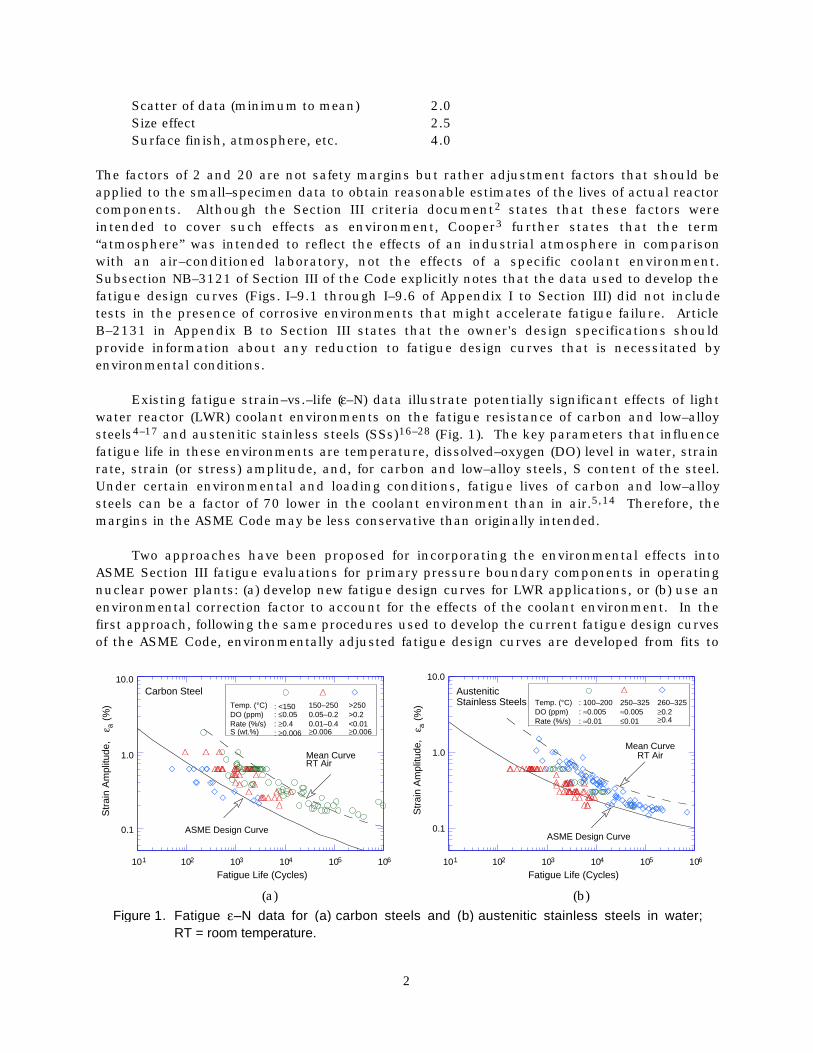
1. Fatigue e–N data for carbon steels and austenitic stainless steels in water............... 2

2. Configuration of fatigue test specimen......................................................................... 5

3. Surface roughness profile of fatigue test specimen. .................................................... 6

4. Autoclave system for fatigue tests in water.................................................................. 6

5. Dependence of fatigue lives of carbon and low–alloy steels on strain rate.................. 11

6. Change in fatigue life of A333–Gr 6 carbon steels with temperature.......................... 12

7. Dependence on dissolved oxygen of fatigue life of carbon steels at 288 and250°C............................................................................................................................. 12

8. Effect of water flow rate on fatigue life of A333–Gr 6 carbon steel in high–puritywater at 289°C and strain amplitude and strain rates of 0.3% and 0.01%/s and0.6% and 0.001%/s...................................................................................................... 13

9. Effect of flow rate on low–cycle fatigue of carbon steel tube bends in high–puritywater at 240°C .............................................................................................................. 14

10. Dependence of fatigue life of austenitic stainless steels on strain rate inlow––DO water .............................................................................................................. 15

11. Dependence of fatigue life of Types 304 and 316NG stainless steel on strain ratein high– and low–DO water at 288°C ........................................................................... 15

12. Dependence of fatigue life of two heats of Type 316NG SS on strain rate inhigh– and low–DO water at 288°C................................................................................ 16

13. Effects of conductivity of water and soaking period on fatigue life of Type 304SS in high–DO water..................................................................................................... 17

14. Change in fatigue lives of austenitic stainless steels in low–DO water withtemperature................................................................................................................... 18

15. Fatigue life of Type 316 stainless steel under constant and varying testtemperature................................................................................................................... 18

16. Effect of surface roughness on fatigue life of A106 Gr B carbon steel and A533low–alloy steel in air and high–purity water at 289°C ................................................. 20

17. Effect of surface roughness on fatigue life of Type 316NG and Type 304stainless steels in air and high–purity water at 289°C................................................ 20

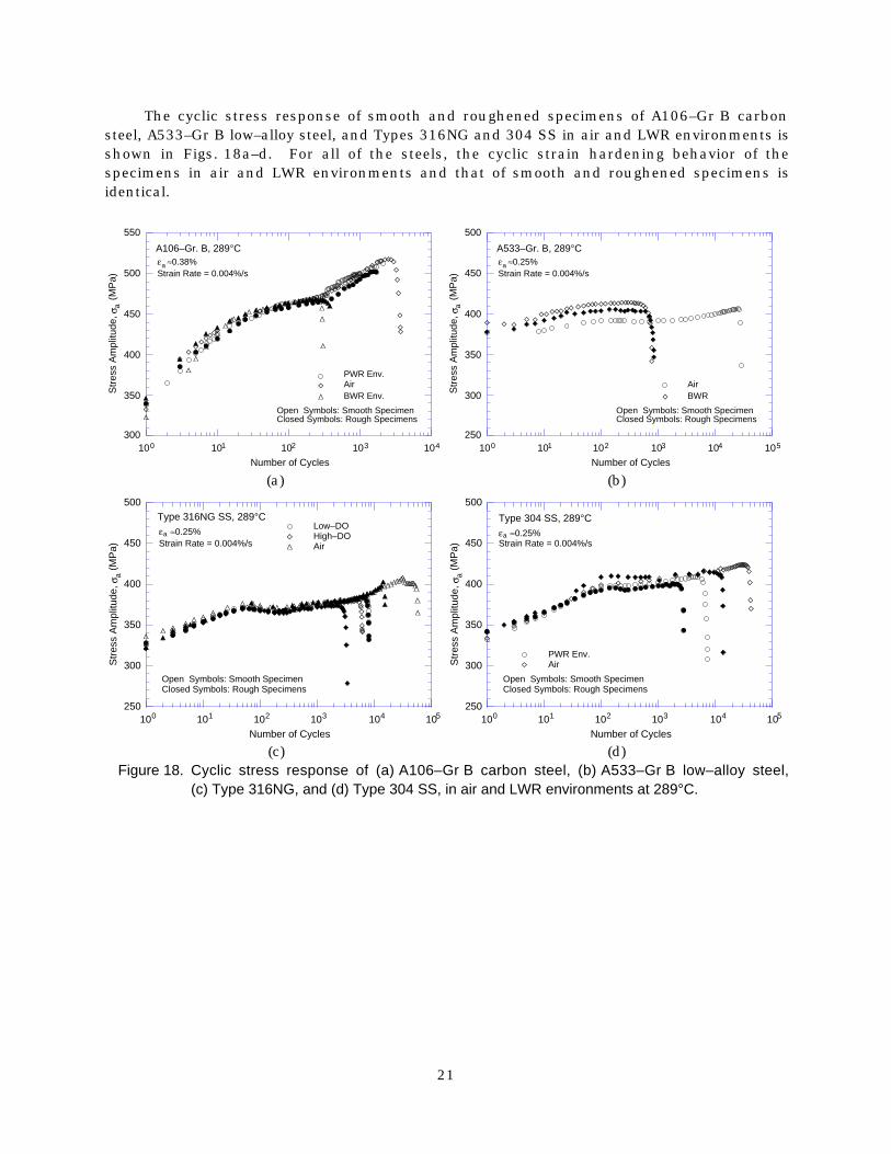
18. Cyclic stress response of A106–Gr B carbon steel, A533–Gr B low–alloy steel,Type 316NG, and Type 304 SS, in air and LWR environments at 289°C. .................. 21

vii

19. Fatigue design curves developed from statistical model for carbon steels andlow–alloy steels under service conditions where one or more critical thresholdvalues are not satisfied................................................................................................. 25

20. Fatigue design curves developed from statistical model for carbon steels andlow–alloy steels in high–DO water at 200, 250, and 288°C and under serviceconditions where all other threshold values are satisfied. .......................................... 26

21. Fatigue design curves developed from the statistical model for austeniticstainless steels in air at room temperature, LWR environments under serviceconditions where one or more critical threshold values are not satisfied, andLWR environments under service conditions where all threshold values aresatisfied. ........................................................................................................................ 27

22. Fatigue data for carbon and low–alloy steel and Type 304 stainless steelcomponents................................................................................................................... 30

23. Estimated cumulative distribution of Parameter A in statistical models forfatigue life for heats of carbon and low–alloy steels and austenitic SSs in airand water environments............................................................................................... 32

24. Schematic illustration of growth of short cracks in smooth specimens as afunction of fatigue life fraction and crack velocity as a function of crack length ....... 37

viii

Tables

1. Composition of austenitic and ferritic steels for fatigue tests .................................... 5

2. Fatigue test results for smooth and rough specimens of austenitic SSs andcarbon and low–alloy steels in air and LWR environments at 288°C......................... 19

3. Values of Parameter A in statistical model for carbon steels as a function ofconfidence level and percentage of population bounded ............................................ 33

4. Values of Parameter A in statistical model for low–alloy steels as a function ofconfidence level and percentage of population bounded ............................................ 33

5. Values of Parameter A in statistical model for austenitic stainless steels as afunction of confidence level and percentage of population bounded.......................... 33

6. Margins on life for carbon steels corresponding to various confidence levels andpercentile values of Parameter A ................................................................................. 34

7. Margins on life for low–alloy steels corresponding to various confidence levelsand percentile values of Parameter A.......................................................................... 34

8. Margins on life for austenitic stainless steels corresponding to variousconfidence levels and percentile values of Parameter A ............................................. 34

9. Factors on cycles and strain or stress to be applied to mean e–N curve.................... 38

ix

Executive Summary

Section III, Subsection NB, of the ASME Boiler and Pressure Vessel Code contains rulesfor the design of Class 1 components of nuclear power plants. Figures I–9.1 through I–9.6 ofAppendix I to Section III specify the Code fatigue design curves for applicable structuralmaterials. However, Section III, Subsection NB–3121, of the Code states that the effects of thecoolant environment on fatigue resistance of a material were not intended to be addressed inthese design curves. Therefore, the effects of environment on the fatigue resistance ofmaterials used in operating pressurized water reactor and boiling water reactor plants, whoseprimary–coolant pressure boundary components were designed in accordance with the Code,are uncertain.

The current Section–III fatigue design curves of the ASME Code were based primarily onstrain–controlled fatigue tests of small polished specimens at room temperature in air. Best–fitcurves to the experimental test data were first adjusted to account for the effects of meanstress and then lowered by a factor of 2 on stress and 20 on cycles (whichever was moreconservative) to obtain the fatigue design curves. These factors are not safety margins butrather adjustment factors that must be applied to experimental data to obtain estimates of thelives of components. They were not intended to address the effects of the coolant environmenton fatigue life. Recent fatigue–strain–vs.–life (e–N) data obtained in the U.S. and Japandemonstrate that light water reactor (LWR) environments can have potentially significanteffects on the fatigue resistance of materials. Specimen lives obtained from tests in simulatedLWR environments can be much shorter than those obtained from corresponding tests in air.

The existing fatigue e–N data for carbon and low–alloy steels and wrought and castaustenitic stainless steels (SSs) have been evaluated to define the effects of key material,loading, and environmental parameters on the fatigue lives of these steels. The fatigue lives ofcarbon and low–alloy steels and austenitic SSs are decreased in LWR environments;environmental effects are significant only when certain critical parameters, e.g., temperature,strain rate, dissolved oxygen (DO) level, and strain amplitude, meet certain threshold values.Environmental effects are moderate when any one of the threshold conditions is not satisfied.The threshold values of the critical parameters and the effects of other parameters, such aswater conductivity, water flow rate, and material heat treatment, on the fatigue life of the steelsare summarized.

Experimental data are presented on the effects of surface roughness on the fatigue life ofcarbon and low–alloy steels and austenitic SSs in air and LWR environments. For austeniticSSs, the fatigue life of roughened specimens is a factor of ª3 lower than it is for the smoothspecimens in both air and low–DO water. The fatigue life of roughened specimens of carbonand low–alloy steels in air is lower than that of smooth specimens; but, in high–DO water thefatigue life of roughened and smooth specimens is the same. In low–DO water, the fatigue lifeof the roughened specimens of carbon and low–alloy steels is slightly lower than that of smoothspecimens.

Statistical models are presented for estimating the fatigue life of carbon and low–alloysteels and wrought and cast austenitic SSs as a function of material, loading, andenvironmental parameters. Also, two approaches are presented for incorporating the effects ofLWR environments into ASME Section III fatigue evaluations. In the first approach,

x

environmentally adjusted fatigue design curves have been developed by adjusting the best–fitexperimental curve for the effect of mean stress and by setting margins of 20 on cycles and 2on strain to account for the uncertainties in life associated with material and loadingconditions. These curves provide allowable cycles for fatigue crack initiation in LWR coolantenvironments. The second approach considers the effects of reactor coolant environments onfatigue life in terms of an environmental correction factor Fen, which is the ratio of fatigue lifein air at room temperature to that in water under reactor operating conditions. To incorporateenvironmental effects into the ASME Code fatigue evaluations, the fatigue usage factor for aspecific load set, based on the current Code design curves, is multiplied by the correctionfactor.

Data available in the literature have been reviewed to evaluate the conservatism in theexisting ASME Code fatigue evaluations. Much of the conservatism in these evaluations arisesfrom current design procedures, e.g., stress analysis rules, and cycle counting. However, theASME Code permits alternative approaches, such as finite–element analyses, fatiguemonitoring, and improved Ke factors, that can significantly decrease the conservatism in thecurrent fatigue evaluation procedures.

Because of material variability, data scatter, and component size and surface, the fatiguelife of actual components differs from that of laboratory test specimens under a similar loadinghistory, and the mean e–N curves for laboratory test specimens must be adjusted to obtaindesign curves for components. These design margins are another source of possibleconservatism. The factors of 2 on stress and 20 on cycles, used in the Code, were intended tocover the effects of variables that can influence fatigue life but were not investigated in thetests that provided the data for the curves. Although these factors were intended to besomewhat conservative, they should not be considered safety margins because they wereintended to account for variables that are known to have effects on fatigue life. This reportpresents a critical review of the ASME Code fatigue design curve margins. Data available in theliterature have been reviewed to evaluate the margins on cycles and stress that are needed toaccount for the effects of size and surface finish and the uncertainties due to materialvariability and data scatter. The results indicate that the current ASME Code requirements ofa factor of 2 on stress and 20 on cycle are quite reasonable, but do not contain excessconservatism that can be assumed to account for the effects of LWR environments. They thusprovide appropriate design margins for the development of design curves from mean datacurves for small specimens in LWR environments.

xi

Acknowledgments

The authors thank Tom Galvin, Jack Tezak, and Ed Listwan for their contributions to theexperimental effort. This work was sponsored by the Office of Nuclear Regulatory Research,U.S. Nuclear Regulatory Commission, under Job Code Y6388; Program Manager:W. H. Cullen, Jr.

1

1 Introduction

Cyclic loadings on a structural component occur because of changes in mechanical andthermal loadings as the system goes from one load set (e.g., pressure, temperature, moment,and force loading) to another. For each load set, an individual fatigue usage factor isdetermined by the ratio of the number of cycles anticipated during the lifetime of thecomponent to the allowable cycles. Figures I–9.1 through I–9.6 of the mandatory Appendix I toSection III of the ASME Boiler and Pressure Vessel Code specify fatigue design curves thatdefine the allowable number of cycles as a function of applied stress amplitude. Thecumulative usage factor (CUF) is the sum of the individual usage factors, and ASME CodeSection III requires that the CUF at each location must not exceed 1.

The ASME Code fatigue design curves, given in Appendix I of Section III, are based onstrain–controlled tests of small polished specimens at room temperature in air. The designcurves have been developed from the best–fit curves to the experimental fatigue–strain–vs.–life(e–N) data that are expressed in terms of the Langer equation1 of the form

eanA N A= ( ) +1 21– , (1)

where ea is the applied strain amplitude, N is the fatigue life, and A1, A2, and n1 arecoefficients of the model. Equation 1 may be written in terms of stress amplitude Sa insteadof ea. The stress amplitude is the product of ea and elastic modulus E, i.e., Sa = E◊ ea. Thecurrent ASME Code best–fit or mean curve for various steels is given by

S

E

N ABa =

-ÊËÁ

ˆ¯̃

+4

100100

ln , (2)

where E is the elastic modulus, N is the number of cycles to failure, and A and B are constantsrelated to reduction in area in a tensile test and endurance limit of the material at 107 cycles,respectively. In the fatigue tests performed during the last three decades, fatigue life is definedin terms of the number of cycles for tensile stress to decrease 25% from its peak or steady statevalue. For a typical specimen diameter used in these studies, this corresponds to the numberof cycles needed to produce an ª 3–mm–deep crack in the test specimen. Thus, the fatigue lifeof a material is actually represented by three parameters, e.g., strain or stress, cycles, andcrack length. The best–fit curve to the existing fatigue e–N data represents, for a given strain orstress amplitude, the number of cycles needed to develop a 3–mm crack.

The ASME Code fatigue design curves have been obtained from the best–fit curves by firstadjusting for the effects of mean stress on fatigue life and then reducing the fatigue life at eachpoint on the adjusted curve by a factor of 2 on strain (or stress) or 20 on cycles, whichever ismore conservative. As described in the Section III criteria document,2 these factors wereintended to account for data scatter (including material variability) and differences in surfacecondition and size between the test specimens and actual components. In comments byCooper3 about the initial scope and intent of the Section III fatigue design procedures it isstated that the factor of 20 on life was regarded as the product of three subfactors:

2

Scatter of data (minimum to mean) 2.0Size effect 2.5Surface finish, atmosphere, etc. 4.0

The factors of 2 and 20 are not safety margins but rather adjustment factors that should beapplied to the small–specimen data to obtain reasonable estimates of the lives of actual reactorcomponents. Although the Section III criteria document2 states that these factors wereintended to cover such effects as environment, Cooper3 further states that the term“atmosphere” was intended to reflect the effects of an industrial atmosphere in comparisonwith an air–conditioned laboratory, not the effects of a specific coolant environment.Subsection NB–3121 of Section III of the Code explicitly notes that the data used to develop thefatigue design curves (Figs. I–9.1 through I–9.6 of Appendix I to Section III) did not includetests in the presence of corrosive environments that might accelerate fatigue failure. ArticleB–2131 in Appendix B to Section III states that the owner's design specifications shouldprovide information about any reduction to fatigue design curves that is necessitated byenvironmental conditions.

Existing fatigue strain–vs.–life (e–N) data illustrate potentially significant effects of lightwater reactor (LWR) coolant environments on the fatigue resistance of carbon and low–alloysteels4–17 and austenitic stainless steels (SSs)16–28 (Fig. 1). The key parameters that influencefatigue life in these environments are temperature, dissolved–oxygen (DO) level in water, strainrate, strain (or stress) amplitude, and, for carbon and low–alloy steels, S content of the steel.Under certain environmental and loading conditions, fatigue lives of carbon and low–alloysteels can be a factor of 70 lower in the coolant environment than in air.5,14 Therefore, themargins in the ASME Code may be less conservative than originally intended.

Two approaches have been proposed for incorporating the environmental effects intoASME Section III fatigue evaluations for primary pressure boundary components in operatingnuclear power plants: (a) develop new fatigue design curves for LWR applications, or (b) use anenvironmental correction factor to account for the effects of the coolant environment. In thefirst approach, following the same procedures used to develop the current fatigue design curvesof the ASME Code, environmentally adjusted fatigue design curves are developed from fits to

0.1

1.0

10.0

101 102 103 104 105 106

Str

ain

Am

plitu

de,

ea (

%)

Carbon Steel

Fatigue Life (Cycles)

Mean CurveRT Air

ASME Design Curve

Temp. (°C)DO (ppm)Rate (%/s)S (wt.%)

: <150: £0.05: ≥0.4: ≥0.006

150–2500.05–0.20.01–0.4≥0.006

>250>0.2<0.01≥0.006

101 102 103 104 105 106

0.1

1.0

10.0

Austenitic Stainless Steels


Mean CurveRT Air

ASME Design Curve

Temp. (°C)DO (ppm)Rate (%/s)

250–325ª0.005£0.01

: 100–200: ª0.005: ª0.01

260–325≥0.2≥0.4

Str

ain

Am

plitu

de,

e a (

%)

(a) (b)

Figure 1. Fatigue e–N data for (a) carbon steels and (b) austenitic stainless steels in water;RT = room temperature.

3

experimental data obtained in LWR environments. Interim fatigue design curves that addressenvironmental effects on the fatigue life of carbon and low–alloy steels and austenitic SSs werefirst proposed by Majumdar et al.29 Fatigue design curves based on a more rigorous statisticalanalysis of experimental data were developed by Keisler et al.30 These design curves havesubsequently been updated on the basis of updated statistical models.14,17,26

The second approach, proposed by Higuchi and Iida,5 considers the effects of reactorcoolant environments on fatigue life in terms of an environmental correction factor Fen, whichis the ratio of fatigue life in air at room temperature to that in water under reactor operatingconditions. To incorporate environmental effects into fatigue evaluations, the fatigue usagefactor for a specific load set, based on the current Code design curves, is multiplied by theenvironmental correction factor. Specific expressions for Fen, based on the Argonne NationalLaboratory (ANL) statistical models14,17,26 and on the correlations proposed by the Ministry ofInternational Trade and Industry (MITI) of Japan,11 have been proposed.

A pressure vessel research council (PVRC) working group has also been compiling andevaluating fatigue e–N data related to the effects of LWR coolant environments on the fatiguelives of pressure boundary materials.31 One of the tasks in the PVRC activity was to define aset of values for material, loading, and environmental variables that lead to “moderate” or“acceptable” effects of environment on fatigue life. A factor of 4 on the ASME mean life waschosen as a working definition of “moderate” or “acceptable” effects of environment, i.e., up to afactor of 4 decrease in fatigue life due to the environment is considered acceptable and does notrequire further fatigue evaluation. The basis for this choice was the above–listed thirdsubfactor, for surface finish, atmosphere, etc. The criterion for “acceptable” environmentaleffects assumes that the current Code design curve includes a factor of 4 to account for theeffects of environment.

This report presents a critical review of the ASME Code fatigue design margins andassesses the conservatism in the current choice of design margins. The existing fatigue e–Ndata for carbon and low–alloy steels and wrought and cast austenitic SSs have been evaluatedto define the effects of key material, loading, and environmental parameters on the fatigue livesof these steels. Statistical models are presented for estimating their fatigue life as a function ofmaterial, loading, and environmental parameters. Both approaches to incorporating the effectsof LWR environments into ASME Section III fatigue evaluations are considered.

5

2 Experimental

Fatigue tests have been conducted to establish the effects of surface finish on the fatiguelife of austenitic SSs and carbon and low–alloy steels in LWR environments. Tests wereconducted on Types 304 and 316NG SS, A106–Gr B carbon steel, and A533–Gr B low–alloysteel; the composition and heat treatments of the steels are given in Table 1. The A106–Gr Bmaterial was obtained from a 508–mm–diameter, Schedule 140 pipe fabricated by the CameronIron Works of Houston, TX. The A533–Gr B material was obtained from the lower head of theMidland reactor vessel, which was scrapped before the plant was completed. The product formfor Types 304 and 316NG SS materials was 76 x 25–mm bar and 25–mm plate, respectively.

Table 1. Composition (wt.%) of austenitic and ferritic steels for fatigue tests

Material Source C P S Si Cr Ni Mn MoCarbon Steel

A106–Gr Ba ANL 0.290 0.013 0.015 0.25 0.19 0.09 0.88 0.05Supplier 0.290 0.016 0.015 0.24 – – 0.93 –

Low–Alloy Steel

A533–Gr Bb ANL 0.220 0.010 0.012 0.19 0.18 0.51 1.30 0.48Supplier 0.200 0.014 0.016 0.17 0.19 0.50 1.28 0.47

Austenitic Stainless Steel

Type 304c Supplier 0.060 0.019 0.007 0.48 18.99 8.00 1.54 0.44

Type 316NGd Supplier 0.015 0.020 0.010 0.42 16.42 10.95 1.63 2.14a 508–mm O.D. schedule 140 pipe fabricated by Cameron Iron Works, Heat J–7201. Actual heat treatment not known.b 162–mm–thick hot–pressed plate from Midland reactor lower head. Austenitized at 871–899°C for 5.5 h and brine

quenched; then tempered at 649–663°C for 5.5 h and brine quenched. The plate was machined to a final thickness of127 mm. The inside surface was inlaid with 4.8–mm weld cladding and stress relieved at 607°C for 23.8 h.

c 76 x 25–mm bar stock, Heat 30956. Solution annealed at 1050°C for 0.5 h.d 25–mm–thick plate, Heat P91576. Solution annealed at 1050°C for 0.5 h.

Smooth cylindrical specimens, with a 9.5–mm diameter and a 19–mm gauge length, wereused for the fatigue tests (Fig. 2). The gauge section of the specimens was oriented along theaxial directions of the carbon steel pipe and along the rolling direction for the bar and plates.The gauge length of all specimens was given a 1–mm surface finish in the axial direction toprevent circumferential scratches that might act as sites for crack initiation. Some specimens

.380

.378.380.378

A .001A .001

.376

.374A .001

.375

.750

1 1/4

5 15/16

11 7/8

1.500 R.750

+.0000-.0005

A .001

.750+.000-.002

A .001

A

Figure 2. Configuration of fatigue test specimen (all dimensions in inches).

6

were intentionally roughened in a lathe, under controlled conditions, with 50–grit sandpaper toproduce circumferential scratches. The measured surface roughness of the specimen is shownin Fig. 3. The average surface roughness (Ra) was 1.2 mm, and the root–mean–square (RMS)value of surface roughness (Rq) was 1.6 mm (61.5 micro–inch).

Tests in water were conducted in a 12–mL autoclave (Fig. 4) equipped with a recirculatingwater system that consisted of a 132–L closed feedwater storage tank, PulsafeederT M

high–pressure pump, regenerative heat exchanger, autoclave preheater, test autoclave,electrochemical potential (ECP) cell, back-pressure regulator, ion exchange bed, 0.2–micronfilter, and return line to the tank. Water was circulated at a rate of ª10 mL/min. Waterquality was maintained by circulating water in the feedwater tank through an ion exchangecleanup system. An Orbisphere meter and CHEMetricsTM ampules were used to measure theDO concentrations in the supply and effluent water. The redox and open–circuit corrosionpotentials were monitored at the autoclave outlet by measuring the ECPs of platinum and an

200 micro inch 0 .005 inch

Figure 3. Surface roughness profile of fatigue test specimen.

Figure 4.Autoclave system for fatigue tests in water.

7

electrode of the test material, respectively, against a 0.1–M KCl/AgCl/Ag external (cold)reference electrode. A detailed description of the test facility has been presented earlier.26,32

Boiling water reactor (BWR) conditions were established by bubbling N2 that contained1–2% O2 through deionized water in the supply tank. The deionized water was prepared bypassing purified water through a set of filters that comprise a carbon filter, an Organex–Qfilter, two ion exchangers, and a 0.2–mm capsule filter. Water samples were taken periodicallyto measure pH, resistivity, and DO concentration. When the desired concentration of DO wasattained, the N2/O2 gas mixture in the supply tank was maintained at a 20–kPa overpressure.After an initial transition period during which an oxide film developed on the fatigue specimen,the DO level and the ECP in the effluent water remained constant. Test conditions aredescribed in terms of the DO in effluent water.

Simulated pressurized water reactor (PWR) water was obtained by dissolving boric acidand lithium hydroxide in 20 L of deionized water before adding the solution to the supply tank.The DO in the deionized water was reduced to <10 ppb by bubbling N2 through the water. Avacuum was drawn on the tank cover gas to speed deoxygenation. After the DO was reducedto the desired level, a 34–kPa overpressure of hydrogen was maintained to provide ª2 ppmdissolved H (or ª23 cc3/kg) in the feedwater.

All tests were conducted at 288°C, with fully reversed axial loading (i.e., R = –1) and atriangular or sawtooth waveform. During the tests in water, performed under stroke control,the specimen strain was controlled between two locations outside the autoclave. Companiontests in air were performed under strain control with an axial extensometer; during the test thestroke at the location used to control the water tests was recorded. Information from the airtests was used to determine the stroke required to maintain constant strain in the specimengauge. To account for cyclic hardening of the material, the stroke that was needed to maintainconstant strain was gradually increased during the test, based on the stroke measurementsfrom the companion strain–controlled tests. The fatigue life N25 is defined as the number ofcycles for tensile stress to decrease 25% from its peak or steady–state value.

9

3 Fatigue eeee–N Data in LWR Environments

The existing fatigue e–N data developed at various establishments and researchlaboratories worldwide have been compiled and categorized according to test conditions. Thefatigue data were obtained on smooth specimens tested under a fully reversed loadingcondition, i.e., load ratio R = –1; tests on notched specimens or at values of R other than –1were excluded. Unless otherwise mentioned, all tests were conducted on gauge specimens instrain control. In nearly all tests, fatigue life is defined as the number of cycles N25 necessaryfor tensile stress to drop 25% from its peak or steady–state value; in some tests, life is definedas the number of cycles for peak tensile stress to decrease by 1–5%. Also, for fatigue tests ontube specimens, life was represented by the number of cycles to develop a leak.

For carbon and low–alloy steels, the primary sources of e–N data include the testsperformed by General Electric Co. (GE) at the Dresden 1 reactor,33,34 work sponsored by theElectric Power Research Institute (EPRI) at GE,4,35 the work of Terrell at Materials EngineeringAssociates (MEA),36,37 the present work at ANL,12–17 the JNUFAD* database, and recentstudies at Ishikawajima–Harima Heavy Industries Co., (IHI), Hitachi, and Mitsubishi HeavyIndustries (MHI) in Japan.5-10 The database is composed of results from ª1400 tests, ª650 inair and ª750 in water. Carbon steels include 8 heats of A333–Grade 6, 3 heats ofA106–Grade B, and a heat each of A516–Grade 70 and A508–Class 1 steel, while the low–alloysteels include 8 heats of A533–Grade B, 10 heats of A508–Class 2 and 3 steels, and a heat ofA302–Grade B.

The relevant fatigue e–N data for austenitic SSs in air include the data compiled by Jaskeand O'Donnell38 for developing fatigue design criteria for pressure vessel alloys, the JNUFADdatabase from Japan, and the results of Conway et al.39 and Keller.40 In water, the existingdata include the tests performed by GE at the Dresden 1 reactor,33 the JNUFAD database,studies at MHI,18,21-23 IHI,19 and Hitachi41,42 in Japan, and the present work at ANL.24-28

In air, the fatigue e–N database for austenitic SSs is composed of 500 tests: 240 on26 heats of Type 304 SS, 170 on 15 heats of Type 316 SS, and 90 on 4 heats of Type 316NG.Most of the tests have been conducted on cylindrical gauge specimens with fully reversed axialloading; ª75 tests were on hourglass specimens, and ª40 data points were from bending testson flat-sheet specimens with rectangular cross section. The results indicate that specimengeometry has little or no effect on the fatigue life of austenitc SSs; the fatigue lives of hourglassspecimens are comparable to those of gauge specimens.

In water, the database for austenitic SSs consists of 310 tests: 150 on 9 heats ofType 304 SS, 60 on 3 heats of Type 316 SS, and 100 on 4 heats of Type 316NG. Nearly 90% ofthe tests in water were conducted at temperatures between 260 and 325°C. The data onType 316NG in water have been obtained primarily at DO levels ≥0.2 ppm and those onType 316 SS, at £0.005 ppm DO; half of the tests on Type 304 SS were at low DO levels, theremaining half, at high DO levels. The existing e–N data for cast SS are very limited, i.e., a totalof 64 tests on 5 heats of CF–8M SS.17,21,22 Nearly 90% of the tests on cast SSs have beenconducted in simulated PWR water at 325°C.

* Private communication from M. Higuchi, Ishikawajima–Harima Heavy Industries Co., Japan, to M. Prager of thePressure Vessel Research Council, 1992. The old data base “FADAL” has been revised and renamed “JNUFAD.”

10

The existing fatigue e–N data, both foreign and domestic, are consistent with each other,and are also consistent with the large database for fatigue crack growth rates (CGRs) obtainedon fracture mechanics specimens. In LWR environments, data on both fatigue crack initiationand fatigue crack growth show similar trends. For example, the effects of loading andenvironmental parameters, such as strain rate, DO level in water, or S content in carbon andlow–alloy steels, are similar for fatigue crack initiation and fatigue crack growth.

The fatigue life of a material, i.e., cycles required to form an ª3–mm–deep crack in thematerial, has traditionally been divided into two stages: an initiation stage that involves thegrowth of microstructurally small cracks (i.e., cracks smaller than ª200 mm), and a propagationstage that involves the growth of mechanically small cracks.15,17,27,43,44 A fracture mechanicsapproach and CGR data have been used to predict fatigue crack initiation in carbon and low-alloy steels in air and LWR environments.17

The decrease in fatigue lives of carbon and low–alloy steels and austenitic SSs in LWRenvironments is caused primarily by the effects of the environment on the growth ofmicrostructurally small cracks and, to a lesser extent, on enhanced growth rates ofmechanically small cracks.17,43,44 In LWR environments, the growth of small cracks in carbonand low–alloy steels occurs by a slip oxidation/dissolution process, and in austenitic SSs, mostlikely, by mechanisms such as H–enhanced crack growth.

3.1 Carbon and Low–Alloy Steels

In air, the fatigue lives of carbon and low–alloy steels depend on steel type, temperature,orientation (rolling or transverse), and strain rate. The fatigue life of carbon steels is a factor ofª1.5 lower than that of low–alloy steels. For both steels, life is decreased by a factor of ª1.5when temperature is increased from room temperature to 288°C. Carbon steels, which have apearlite and ferrite structure and low yield stress, exhibit significant initial hardening. Thelow–alloy steels, which have a tempered bainite and ferrite structure and relatively high yieldstress, exhibit little or no initial hardening and may exhibit softening. In the temperaturerange of dynamic strain aging (200–370°C), these steels show negative sensitivity to strain rate,i.e., cyclic stresses increase with decreasing strain rate. Cyclic–stress–vs.–strain curves forcarbon and low–alloy steels at 288°C have been developed as a function of strain rate.12–17

The effect of strain rate on fatigue life is not clear; for some heats, life may be unaffected ordecrease, for other heats, it may increase. Also, depending on the distribution and morphologyof sulfides, fatigue properties in the transverse orientation may be inferior to those in therolling orientation. The ASME mean curve for low–alloy steels is in good agreement with theexperimental data. The corresponding curve for carbon steels is somewhat conservative,especially at strain amplitudes <0.2%.

The fatigue lives of carbon and low–alloy steels are reduced in LWR environments.Although the microstructures and cyclic–hardening behavior of carbon steels and low–alloysteels differ significantly, the effects of the environment on the fatigue life of these steels arevery similar. The magnitude of the reduction depends on temperature, strain rate, DO level inwater, and S content of the steel. The decrease is significant only when four conditions aresatisfied simultaneously, viz., when the strain amplitude, temperature, and DO in water areabove certain threshold values, and the strain rate is below a threshold value. For both steels,only a moderate decrease in life (by a factor of <2) is observed when any one of the thresholdconditions is not satisfied. The S content of the steel is also important; its effect on life appears

11

to depend on the DO level in water. The threshold values and the effects of the criticalparameters on fatigue life are summarized below.

Strain: A minimum threshold strain is required for an environmentally assisted decreasein the fatigue lives of carbon and low–alloy steels.13–17 The threshold strain is defined as theminimum total applied strain above which environmental effects on fatigue life are significant.Even within a given loading cycle, environmental effects are significant at strain levels greaterthan the threshold value. Limited data suggest that the threshold value is ª20% higher thanthe fatigue limit for the steel. The results also indicate that, within a given loading cycle,environmental effects are significant primarily during the tensile–loading cycle. This can beimportant if the strain rate varies over the loading cycle. Thus, for example, low strain rates atstrains lower than the threshold strain and high strain rates for those portions of the cycle atstrains greater than the threshold strain would not lead to significant reductions in life.Consequently, it is the loading and environmental conditions, e.g., strain rate, temperature,and DO level, during the tensile–loading cycle that are important for estimating environmentaleffects. Limited data indicate that hold periods during peak tensile or compressive strain haveno effect on the fatigue life of these steels.14

Strain Rate: When all other threshold conditions are satisfied, fatigue life decreaseslogarithmically with decreasing strain rate below 1%/s.5,7,9 The effect of environment on lifesaturates at ª0.001%/s (Fig. 5).12–17 When any one of the threshold conditions is not satisfied,e.g., DO <0.04 ppm or temperature <150°C, the effects of strain rate are consistent with thoseobserved in air. Therefore, heats that are sensitive to strain rate in air show a decrease in lifein water, although the decreases are much smaller than those observed when the thresholdconditions are met.

102

103

104

10-5 10-4 10-3 10-2 10-1 100

AirSimulated PWRª0.7 ppm DO

Fat

igue

Life

(C

ycle

s)

Strain Rate (%/s)

A106–Gr B Carbon Steel

288°C, ea ª0.4%

102

103

104

10-5 10-4 10-3 10-2 10-1 100

AirSimulated PWRª0.7 ppm DO

Fat

igue

Life

(C

ycle

s)

Strain Rate (%/s)

A533–Gr B Low–Alloy Steel

288°C, ea ª0.4%

(a) (b)Figure 5. Dependence of fatigue lives of (a) carbon and (b) low–alloy steels on strain rate (Refs. 12–17).

Temperature: Experimental data indicate a threshold temperature of 150°C, below whichenvironmental effects on life either do not occur or are insignificant. When other thresholdconditions are satisfied, fatigue life decreases linearly with temperature above 150°C and up to320°C (Fig. 6).5,7,9 Fatigue life is insensitive to temperatures below 150°C or highertemperatures when any other threshold condition is not satisfied. Analyses of the fatigue e–Ndata using artificial neural networks also show a similar effect of temperature on the fatiguelives of carbon and low–alloy steels.45 For service histories that involve variable loading

12

conditions, service temperature may be represented by the average of the maximumtemperature and higher of the minimum temperature or 150°C.8

Dissolved Oxygen in Water: When the other threshold conditions are satisfied, fatigue lifedecreases logarithmically with DO above 0.04 ppm; the effect saturates at ª0.5 ppm DO(Fig. 7).7,9 Only a moderate decrease in life, i.e., less than a factor of 2, is observed at DOlevels below 0.04 ppm. In contrast, environmental enhancement of CGRs has been observed inlow–alloy steels even in low–DO environments.46 This apparent inconsistency of fatigue e–Ndata with the CGR data may be attributed to differences in the environment at the crack tip.The initiation of environmentally assisted enhancement of CGRs in low–alloy steels requires acritical level of sulfides at the crack tip.46 The development of this critical sulfide concentrationrequires a minimum crack extension of 0.33 mm and CGRs of 1.3x10–4–4.2x10–7 mm/s.These conditions are not achieved under typical e-N tests. Thus, environmental effects onfatigue life are expected to be insignificant in low–DO environments.

Water Conductivity: In most studies the DO level in water has generally been consideredthe key environmental parameter that affects fatigue life of materials in LWR environments.

0 50 100 150 200 250 300 350

0.004%/s (>1 ppm DO)0.004%/s (0.05 ppm DO)0.002%/s (>1 ppm DO)0.4%/s (Air)

102

103

104

Temperature (°C)

A333–Gr 6 Carbon Steelea = 0.6%, S = 0.012 wt.%

Strain Rate

Fat

igue

Life

(C

ycle

s)

0 50 100 150 200 250 300 350

>1 ppm<0.05 ppmAir 0.4 or 0.01%/s)

102

103

104

Temperature (°C)

A333–Gr 6 Carbon Steelea = 0.6%, S = 0.015 wt.%

Strain Rate = 0.01%/s

Dissolved OxygenFat

igue

Life

(C

ycle

s)

Figure 6. Change in fatigue life of A333–Gr 6 carbon steels with temperature (Refs. 5,7,9).

102

103

104

10-3 10-2 10-1 100 101

0.004 (0.012% S)0.01 (0.015% S)0.002 (0.012% S)

Fat

igue

Life

(C

ycle

s)

Dissolved Oxygen (ppm)

A333-6 Steel 288°CStrain Amplitude: 0.6%

Strain Rate (%/s)

102

103

104

10-3 10-2 10-1 100 101

0.004 (0.012% S)0.01 (0.015% S)0.002 (0.012% S)

Fat

igue

Life

(C

ycle

s)

Dissolved Oxygen (ppm)

A333-6 Steel 250°CStrain Amplitude: 0.6%

Strain Rate (%/s)

(a) (b)Figure 7. Dependence on dissolved oxygen of fatigue life of carbon steels at (a) 288 and (b) 250°C

(Refs. 7,9).

13

Studies on the effect of other parameters, such as the concentration of anionic impurities inwater (expressed as the overall conductivity of water), are somewhat limited. Studies on theeffect of conductivity on the fatigue life indicate that the fatigue life of WB36 low–alloy steel at177°C in water with ª8 ppm DO decreased by a factor of ª6 when the conductivity of water wasincreased from 0.06 to 0.5 mS/cm.47,48 A similar behavior has also been observed in anotherstudy of the effect of conductivity on the initiation of short cracks.49

Sulfur Content of Steel: The effect of S content on fatigue life appears to depend on the DOcontent of the water. When the threshold conditions are satisfied, the fatigue life decreaseswith increasing S content for DO levels £1.0 ppm. Limited data suggest that environmentaleffects on life saturate at a S content of ª0.015 wt.%.14 For DO levels >1.0 ppm, fatigue lifeseems to be relatively insensitive to S content in the range of 0.002–0.015 wt.%.11

Flow Rate: Nearly all of the fatigue e–N data for LWR environments have been obtained atvery low water flow rates. Recent data indicate that, under the environmental conditionstypical of operating BWRs, environmental effects on the fatigue life of carbon steels are at leasta factor of 2 lower at high flow rates (7 m/s) than at 0.3 m/s or lower.50–52 The beneficialeffects of increased flow rate are greater for high–S steels and at low strain rates.50,51 Theeffect of water flow rate on the fatigue life of high–S (0.016 wt.%) A333–Gr 6 carbon steel inhigh–purity water at 289°C is shown in Fig. 8. At 0.3% strain amplitude, 0.01%/s strain rate,and all DO levels, fatigue life is increased by a factor of ª2 when the flow rate is increased fromª10–5 to 7 m/s. At 0.6% strain amplitude and 0.001%/s strain rate, fatigue life is increased bya factor of ª6 in water with 0.2 ppm DO and by a factor of ª3 in water with 1.0 or 0.05 ppmDO. Under similar loading conditions, i.e., 0.6% strain amplitude and 0.001%/s strain rate, alow–S (0.008 wt.%) heat of A333–Gr 6 carbon steel showed only a factor of ª2 increase infatigue life with increased flow rates. Note that the beneficial effects of flow rate are determinedfrom a single test on each material at very low flow rates; data scatter in LWR environments istypically a factor of ª2.

A factor of 2 increase in fatigue life was observed (Fig. 9) at Kraftwerk Union laboratories(KWU) during component tests with 180° bends of carbon steel tubing (0.025 wt.% S) when

102

103

104

10-5 10-4 10-3 10-2 10-1 100 101

1.00.20.05

Fat

igue

Life

(C

ycle

s)

Flow Rate (m/s)

A333–Gr 6 Carbon Steel (High–S)

289°CStrain Amplitude 0.3%Strain Rate 0.01%/s

DO (ppm)

101

102

103

104

10-5 10-4 10-3 10-2 10-1 100 101

1.00.20.05

Fat

igue

Life

(C

ycle

s)

Flow Rate (m/s)

A333–Gr 6 Carbon Steel (High–S)

289°CStrain Amplitude 0.6%Strain Rate 0.001%/s

DO (ppm)

(a) (b)Figure 8. Effect of water flow rate on fatigue life of A333–Gr 6 carbon steel in high–purity water at

289°C and strain amplitude and strain rates of (a) 0.3% and 0.01%/s and (b) 0.6% and0.001%/s (Ref. 50,51).

14

internal flow rates of up to 0.6 m/s were established.52 The tests were conducted at 240°C inwater that contained 0.2 ppm DO.

3.2 Austenitic Stainless Steels

In an air environment, the fatigue life of Type 304 SS is comparable to that of Type 316SS; the fatigue life of Type 316NG is slightly higher than that of Types 304 and 316 SS,particularly at high strain amplitudes. The results also indicate that the fatigue life ofaustenitic SSs in air is independent of temperature from room temperature to 427°C. Althoughthe effect of strain rate on fatigue life seems to be significant at temperatures above 400°C,variations in strain rate in the range of 0.4–0.008%/s have no effect on the fatigue lives of SSsat temperatures up to 400°C.53 The fatigue e–N behavior of cast CF–8 and CF–8M SSs issimilar to that of wrought austenitic SSs.26 Under cyclic loading, austenitic SSs exhibit rapidhardening during the first 50–100 cycles; the extent of hardening increases with increasingstrain amplitude and decreasing temperature and strain rate.26,53 The initial hardening isfollowed by softening and a saturation stage at high temperatures, and by continuous softeningat room temperature. The ASME Code mean curve is not consistent with the existing fatiguee–N data for austenitic SSs. At strain amplitudes <0.5%, the mean curve predicts significantlylonger fatigue lives than those observed experimentally.

The fatigue lives of austenitic SSs are also decreased in LWR environments. Themagnitude of this reduction depends on strain amplitude, strain rate, temperature, DO level inthe water, and, possibly, the composition and heat treatment of the steel.16–28 The effects ofLWR environments on the fatigue lives of wrought materials are comparable for Types 304,316, and 316NG SSs; effects on cast materials differ somewhat. As in the case of the carbonand low–alloy steels, fatigue life is reduced significantly only when certain critical parametersmeet certain threshold values. The critical parameters that influence fatigue life and thethreshold values that are required for environmental effects to be significant are summarizedbelow.

Strain Amplitude: As in the case of the carbon and low–alloy steels, a minimum thresholdstrain is required for the environmentally induced decrease in fatigue lives of SS to occur. Thethreshold strain appears to be independent of material type (weld or base metal) andtemperature in the range of 250–325°C, but it tends to decrease as the strain amplitude of the

0.1

1.0

101 102 103 104

0.2 ppm0.01 ppmS

trai

n A

mpl

itude

, e a

(%

)


Carbon Steel (0.025% S)240°C, Strain Rate: 0.001%/s

Best–Fit Curve RT Air

ASME CodeDesign Curve

Open Symbols: Low flowClosed Symbols: 0.6 m/s flow rate

Dissolved Oxygen

Figure 9.Effect of flow rate on low–cycle fatigue ofcarbon steel tube bends in high–purity waterat 240°C (Ref. 52).

15

cycle is decreased.23 The threshold strain appears to be related to the elastic strain range ofthe material23 and does not correspond to the rupture strain of the surface oxide film.

Hold–Time Effects: For a given loading cycle, environmental effects are significantprimarily during the tensile–loading cycle, and at strain levels greater than the threshold value.Consequently, loading and environmental conditions, e.g., strain rate, temperature, and DOlevel, during the tensile–loading cycle are important for environmentally assisted reduction ofthe fatigue lives of these steels. Limited data indicate that hold periods during peak tensile orcompressive strain have no effect on the fatigue life of austenitic SSs. The fatigue lives ofType 304 SS tested in high–DO water with a trapezoidal waveform (i.e., hold periods at peaktensile and compressive strain)33 are comparable to those tested with a triangular waveform.19

Strain Rate: Fatigue life decreases with decreasing strain rate. In low–DO PWRenvironments, fatigue life decreases logarithmically with decreasing strain rate below ª0.4%/s;the effect of environment on life saturates at ª0.0004%/s (Fig. 10).17–27 Only a moderatedecrease in life is observed at strain rates >0.4%/s. A decrease in strain rate from 0.4 to0.0004%/s decreases the fatigue life of austenitic SSs by a factor of ª10. For some SSs, theeffect of strain rate may be less pronounced in high– than in low–DO water (Fig. 11). For cast

102

103

104

10-5 10-4 10-3 10-2 10-1 100

0.380.25

Fat

igue

Life

(C

ycle

s)

Strain Rate (%/s)

288°C; DO £ 0.005 ppmOpen Symbols: Type 304Closed Symbols: Type 316NG

Strain Amplitude (%)

102

103

104

10-5 10-4 10-3 10-2 10-1 100

0.600.300.25

Fat

igue

Life

(C

ycle

s)

Strain Rate (%/s)

325°C; DO £ 0.005 ppmOpen Symbols: Type 304Closed Symbols: Type 316

Strain Amplitude (%)

Figure 10. Dependence of fatigue life of austenitic stainless steels on strain rate in low––DO water(Refs. 26,27).

102

103

104

105

10-5 10-4 10-3 10-2 10-1 100

ª0.38%ª0.25%F

atig

ue L

ife (

Cyc

les)

Strain Rate (%/s)

Type 304 SS288°C

Open Symbols: <0.005 ppm DOClosed Symbols: ª0.7 ppm DO

Strain Amplitude

102

103

104

105

10-5 10-4 10-3 10-2 10-1 100

ª0.4%ª0.25%F

atig

ue L

ife (

Cyc

les)

Strain Rate (%/s)

Type 316NG SS (Heat D432804)288°C

Open Symbols: <0.005 ppm DOClosed Symbols: >0.2 ppm DO

Strain Amplitude

(a) (b)Figure 11. Dependence of fatigue life of Types (a) 304 and (b) 316NG stainless steel on strain rate in

high– and low–DO water at 288°C (Ref. 27).

16

SSs, the effect of strain rate on fatigue life is the same in low– and high–DO water and iscomparable to that observed for the wrought SSs in low–DO water.21,22

Dissolved Oxygen in Water: In contrast to the behavior of carbon and low–alloy steels, thefatigue lives of nonsensitized wrought and cast austenitic SSs are decreased significantly evenin low–DO (i.e., <0.01 ppm DO) water. The decrease in life is greater at low strain rates andhigh temperatures.17–26 Environmental effects on the fatigue lives of these steels in high–DOwater may be influenced by the composition and heat treatment of the steel. At temperaturesabove 150°C, the fatigue lives of wrought SSs in high–DO water are either comparable to21,22

or, in some cases, smaller26 than those in low–DO water.

In high–DO water, only moderate environmental effects were observed for a heat ofType 304 SS when the conductivity of the water was maintained at <0.1 mS/cm and the ECP ofthe steel was above 150 mV.17 During laboratory tests, the time to reach these stableenvironmental conditions depends on test parameters such as the autoclave volume, flow rate,etc. In the ANL test facility, fatigue tests on austenitic SSs in high–DO water required asoaking period of 5–6 days for the ECP of the steel to stabilize. The steel ECPs increased fromzero or negative values to above 150 mV during this period. The fatigue lives of Type 304 SSspecimens, soaked for ª5 days in high–DO water before testing in high–DO water at 289°C andª0.38 and 0.25% strain amplitude, are plotted as a function of strain rate in Fig. 11a. For thisheat, fatigue life decreases linearly with decreasing strain rate in low–DO water, whereas inhigh–DO water, strain rate has no effect on fatigue life. For example, the fatigue life at ª0.38%strain amplitude and 0.0004%/s strain rate is ª1500 cycles in low–DO water and >7300 cyclesin high–DO water. At all strain rates, the fatigue life of Type 304 SS is 30% lower in high–DOwater than in air. However, the results obtained at MHI, Japan, on Types 304 and 316 SSshow a different behavior; environmental effects are observed to be the same in high– andlow–DO water.21–23 As discussed below the different behavior is most likely due to differencesin the steel composition or heat treatment.

For a heat of Type 316NG (Heat D432804), some effect of strain rate is observed inhigh–DO water, although it is smaller than that in low–DO water (Fig. 11b). The Type 316NGspecimens were soaked for only 24 h before testing, thus, environmental conditions may nothave been stable for these tests. To determine the possible influence of the shortersoak–period, additional tests were conducted on another heat of Type 316NG (Heat P91576);these specimens were soaked for ª10 days before testing to achieve stable values for the ECP of

103

104

105

10-3 10-2 10-1 100

Heat D432804Heat P91576, Mill AnnealedHeat P91576 , Solution Annealed

Fat

igue

Life

(C

ycle

s)

Strain Rate (%/s)

Type 316NG SS, 288°CStrain Amp. ª0.25%

Open Symbols: <0.005 ppm DOClosed Symbols: >0.2 ppm DO

Figure 12.Dependence of fatigue life of two heats ofType 316NG SS on strain rate in high– andlow–DO water at 288°C.

17

the steel. The results are shown in Fig. 12. Unlike the data obtained earlier on Heat D432804(diamond symbols), the results for Heat P91576 (triangle symbols) indicate that the fatigue lifeof this heat is the same in low– and high–DO water. These results indicate that, in high–DOwater, material heat treatment may influence the fatigue life of austenitic SSs.

In low–DO water, the fatigue lives of cast SSs are comparable to those of wroughtaustenitic SSs.21–26 Limited data suggest that the fatigue lives of cast SSs in high–DO waterare approximately the same as those in low–DO water.26

Water Conductivity: The effect of the conductivity of water and the ECP of the steel on thefatigue life of austenitic SSs is shown in Fig. 13. In high–DO water, fatigue life is decreased bya factor of ª2 when the conductivity of water is increased from ª0.07 to 0.4 mS/cm. Note thatenvironmental effects appear more significant for the specimens that were soaked for only24 h. For these tests, the ECP of steel was initially very low and increased during the test.

103

104

10-2 10-1 100

Fat

igue

Life

(C

ycle

s)

Conductivity of Water (mS/cm)

Air

Simulated PWR

Type 304 SS 288°CStrain range ª0.77%Strain rate tensile 0.004%/s & compressive 0.4 %/sDO ª0.8 ppm

Open Symbols: ECP 155 mV (ª120 h soak)Closed Symbols: ECP 30–145 mV (ª24 h soak)

Figure 13.Effects of conductivity of water and soakingperiod on fatigue life of Type 304 SS inhigh–DO water (Ref. 17).

Temperature: The data suggest a lower threshold temperature of 150°C (Fig. 14). Abovethis temperature, the environment decreases fatigue life in low–DO water if the strain rate isbelow the threshold of 0.4%/s.11,19 In the range of 150–325°C, the logarithm of fatigue lifedecreases linearly with temperature. Only a moderate decrease in life is observed in water attemperatures below the threshold value of 150°C.

The results of fatigue tests on Type 316 SS under combined mechanical and thermalcycling are presented in Fig. 15 with the data obtained from tests at constant temperature.Two temperature cycling sequences were examined: an in–phase sequence, in whichtemperature cycling was synchronized with mechanical strain cycling, and an out–of–phasesequence in which temperature and strain were out of phase, i.e., maximum temperatureoccurred at minimum strain level and vice versa.20 Two temperature ranges, 100–325°C and200–325°C, were selected for the tests.

As discussed earlier, the tensile load cycle is primarily responsible for environmentallyassisted reduction of fatigue life, and the applied strain and temperature must be above aminimum threshold value for environmental effects to occur. Thus, life should be longer forout–of–phase tests than for in–phase tests, because applied strains above the threshold strainoccur at high temperatures for in–phase tests, whereas applied strains above the thresholdstrain occur only at low temperatures for out–of–phase tests. In Fig. 15, the data for the

18

thermal cycling tests are plotted in terms of an average temperature, i.e., the average of thetemperature at peak strain and the temperature at threshold strain or 150°C (whichever ishigher). From Eq. 3, the threshold strain for this test is 0.46%. Thus, for the temperaturerange of 100–325°C, the temperature plotted in Fig. 15 is the average of 239 and 150°C for theout–of–phase test and the average of 186 and 325°C for the in–phase test. For the temperaturerange of 200–325°C, the temperature plotted in Fig. 15 is the average of 277 and 200°C for theout–of–phase test and the average of 248 and 325°C for the in–phase test. With this choice ofaverage temperatures, the results from thermal cycling tests agree well with those fromconstant–temperature tests (open circles in Fig. 15). The data suggest a linear decrease inlogarithmic life at temperatures above 150°C.

102

103

104

0 50 100 150 200 250 300 350

Constant (0.01)In phase (0.002)Out of phase (0.002)

Fat

igue

Life

(C

ycle

s)

Temperature (°C)

Type 316 SS 325°Cea = 0.6%

DO = <0.005 ppmStrain Rate 0.002%/s

Temperature (Strain Rate, %/s)

Figure 15.Fatigue life of Type 316 stainless steelunder constant and varying test temperature(Ref. 20).

Sensitization Anneal: In low–DO water, a sensitization anneal has no effect on the fatiguelife of Types 304 and 316 SS, whereas, in high–DO water, environmental effects in sensitizedsteels are enhanced. For example, the fatigue life of sensitized steel is a factor of ª2 lower thanthat of solution–annealed material in high–DO water.21,22 Sensitization has little or no effecton the fatigue life of Type 316NG SS in low– and high–DO water.

To investigate the effect of heat treatment, a specimen of Heat P91576 was solutionannealed in the laboratory and tested in high–DO water at 289°C. The fatigue life of the

103

104

50 100 150 200 250 300 350 400

0.4%/s0.01%/s

Fat

igue

Life

(C

ycle

s)

Temperature (°C)

Austenitic SSsea = 0.3%, DO £ 0.005 ppm

Open Symbols: Type 304Closed Symbols: Type 316 & 316NG

103

104

50 100 150 200 250 300 350 400

0.4%/s0.01%/s

Fat

igue

Life

(C

ycle

s)

Temperature (°C)

Austenitic SSse a = 0.6%, DO £ 0.005 ppm

Open Symbols: Type 304Closed Symbols: Type 316 & 316NG

Figure 14. Change in fatigue lives of austenitic stainless steels in low–DO water with temperature(Refs. 17,19–22,26,27).

19

solution–annealed specimen (inverted triangle symbol in Fig. 12) is a factor of ª2 higher thanthat of the mill–annealed specimens. These results indicate that, in high–DO water, materialheat treatment has a strong effect on the fatigue life of austenitic SSs, e.g., environmentaleffects may be significant even for mill–annealed steel where no sensitization is apparent.

Flow Rate: Limited data indicate that the water flow rate has no effect on the fatigue life ofaustenitic SSs in high–purity water at 289°C. The fatigue lives of Type 316NG at 0.6% strainamplitude and 0.001%/s strain rate, in high–purity water with 0.2 or 0.05 ppm DO at 289°C,showed little or no change when the flow rate was increased from ª10–5 to 10 m/s.51 Theresults at 0.3% strain amplitude and 0.01%/s strain rate show slight decrease in fatigue liveswith increasing flow rate. Because the mechanism of fatigue crack initiation in LWRenvironments appears to be different in SSs than in carbon steels, the effect of flow rate is alsolikely to be different.

3.3 Effects of Surface Finish

Several fatigue tests have been conducted on rough specimens at 288°C in air and high–and low–DO water environments. The results of these tests and data obtained earlier onsmooth specimens are presented in Table 2.

Table 2. Fatigue test results for smooth and rough specimens of austenitic SSs and carbon andlow–alloy steels in air and LWR environments at 288°C

TestNo.

Dis.Oxygena

(ppb)Specimen

Type

Dis.Hydrogen(cc/kg)

Li(ppm)

Boron(ppm)

pHat RT

Conduc-tivityb

(mS/cm)

ECP SSa

mV(SHE)

Ten.Ratec

(%/s)

StressAmp.(MPa)

StrainAmp.(%)

LifeN25

(Cycles)A106–Gr B Carbon Steel (Heat J–7201)1621 Air Env. Smooth – – – – – – 1.0E-2 393.5 0.20 38,1281876 Air Env. Rough – – – – – – 1.0E-2 388.9 0.20 11,2701679 3 Smooth 23 2 1000 6.5 20.41 –690 4.0E-3 502.9 0.38 2,1411886 5 Rough – – – 7.3 0.06 –645 4.0E-3 492.4 0.39 1,7651614 400 Smooth – – – 5.9 0.11 84 4.0E-3 465.2 0.39 3031682 700 Smooth – – – 6.0 0.09 185 4.0E-3 460.5 0.37 4691885 740 Rough – – – 6.0 0.06 112 4.0E-3 467.0 0.39 3901624 800 Smooth – – – 5.9 0.10 189 4.0E-3 387.9 0.23 2,2761877 780 Rough – – – 6.5 0.06 138 4.0E-3 381.7 0.22 2,3501884 920 Rough – – – 6.8 0.06 96 4.0E-3 391.2 0.21 2,320A533–Gr B Low–Alloy Steel (Midland Reactor)1627 800 Smooth – – – 5.9 0.10 214 4.0E-3 413.4 0.27 7691887 750 Rough – – – 6.6 0.06 153 4.0E-3 404.0 0.26 842Type 304 Stainless Steel (Heat 30956)1817 Air Env. Smooth – – – – – – 4.0E-3 215.8 0.25 42,1801874 Air Env. Rough – – – – – – 4.0E-3 206.5 0.25 13,9001823 3 Smooth 23 2 1000 6.6 23.06 –699 4.0E-3 204.1 0.25 6,9001875 2 Rough – – – 5.8 0.06 –595 4.0E-3 199.5 0.26 2,280Type 316NG Stainless Steel (Heat P91576)1878 Air Env. Smooth – – – – – – 4.0E-3 200.5 0.25 58,3001890 Air Env. Rough – – – – – – 4.0E-3 195.6 0.25 15,5701879 4 Smooth – – – – 0.06 –591 4.0E-3 190.1 0.25 8,3101889 5 Rough – – – – 0.06 –672 4.0E-3 186.3 0.25 3,2301881 830 Smooth – – – 6.5 0.06 130 4.0E-3 188.3 0.25 6,2001882 760 Smooth – – – 6.5 0.06 140 4.0E-3 190.8 0.25 7,7801888 690 Rough – – – 6.7 0.06 116 4.0E-3 190.5 0.25 8,040aMeasured in effluent.bMeasured in feedwater supply tank.cStrain rate during tensile half of the cycle; rates during compressive half were 0.4%/s for all tests.

20

The results for A106–Gr B carbon steel and A533–Gr B low–alloy steel are shown inFigs. 16a and b, respectively. In air, the fatigue life of rough A106–Gr B specimens is a factorof 3 lower than that of smooth specimens, and, in high–DO water, it is the same as that ofsmooth specimens. In low–DO water, the fatigue life of the roughened A106–Gr B specimen isslightly lower than that of smooth specimens. The effect of surface roughness on the fatiguelife of A533–Gr B low–alloy steel is similar to that for A106–Gr B carbon steel; in high–DOwater, the fatigue lives of both rough and smooth specimens are the same. The results forcarbon and low–alloy steels are consistent with a mechanism of growth by a slipoxidation/dissolution process, which seems unlikely to be affected by surface finish. Becauseenvironmental effects are moderate in low–DO water, surface roughness would be expected toinfluence fatigue life.

The results for Types 316NG and 304 SS are shown in Figs. 17a and b, respectively. Forboth steels, the fatigue life of roughened specimens is lower than that of the smooth specimensin air and low–DO water environments. In high–DO water, the fatigue life is the same for roughand smooth specimens.

0.1

1.0

103 104 105 106

AirPWRBWR

AirPWRBWR

Str

ain

Am

plitu

de,

e a (

%)


Type 316NG SS289°C

Open Symbols: Smooth SpecimensClosed Symbols: Rough Surface, 50 grit paper

Best–Fit Air


Heat D432804 Heat P91576

Strain Rate: 0.004%/s in Water0.4 - 0.004%/s in Air

0.1

1.0

103 104 105 106

AirSimulated PWR Water

Str

ain

Am

plitu

de,

e a (

%)


Type 304 SS289°C


Best–Fit Air


Sawtooth WaveformStrain Rate = 0.004/0.4%/s

(a) (b)Figure 17. Effect of surface roughness on fatigue life of (a) Type 316NG and (b) Type 304 stainless

steels in air and high–purity water at 289°C.

0.1

1.0

102 103 104 105 106

Air, 0.004%/sAir, 0.01%/sª700 ppb DO Water, 0.004%/s5 ppb DO Water, 0.004%/s

Str

ain

Am

plitu

de,

e a (

%)


A106 Gr B Carbon Steel289°C




0.1

1.0

102 103 104 105 106

Air, 0.004%/sAir, 0.4%/sª700 ppb DO Water, 0.004%/s

Str

ain

Am

plitu

de,

e a (%

)


A533 Gr B Low-Alloy Steel289°C




(a) (b)Figure 16. Effect of surface roughness on fatigue life of (a) A106–Gr B carbon steel and (b) A533

low–alloy steel in air and high–purity water at 289°C.

21

The cyclic stress response of smooth and roughened specimens of A106–Gr B carbonsteel, A533–Gr B low–alloy steel, and Types 316NG and 304 SS in air and LWR environments isshown in Figs. 18a–d. For all of the steels, the cyclic strain hardening behavior of thespecimens in air and LWR environments and that of smooth and roughened specimens isidentical.

300

350

400

450

500

550

100 101 102 103 104

PWR Env.AirBWR Env.

Str

ess

Am

plitu

de, s

a (

MP

a)

Number of Cycles

A106–Gr. B, 289°Cea ª0.38%Strain Rate = 0.004%/s

Open Symbols: Smooth SpecimenClosed Symbols: Rough Specimens

250

300

350

400

450

500

100 101 102 103 104 105

AirBWR

Str

ess

Am

plitu

de, s

a (

MP

a)Number of Cycles

A533–Gr. B, 289°Cea ª0.25%Strain Rate = 0.004%/s


(a) (b)

250

300

350

400

450

500

100 101 102 103 104 105

Low–DOHigh–DOAir

Str

ess

Am

plitu

de, s

a (M

Pa)

Number of Cycles

Type 316NG SS, 289°Cea ª0.25%Strain Rate = 0.004%/s


250

300

350

400

450

500

100 101 102 103 104 105

PWR Env.AirS

tres

s A

mpl

itude

, sa (

MP

a)

Number of Cycles

Type 304 SS, 289°Cea ª0.25%Strain Rate = 0.004%/s


(c) (d)Figure 18. Cyclic stress response of (a) A106–Gr B carbon steel, (b) A533–Gr B low–alloy steel,

(c) Type 316NG, and (d) Type 304 SS, in air and LWR environments at 289°C.

23

4 Statistical Models

Statistical models based on the existing fatigue e–N data have been developed at ANL forestimating the fatigue lives of carbon and low–alloy steels and wrought and cast austenitic SSsin air and LWR environments.14,17,26,28 In room–temperature air, the fatigue life N of carbonsteels is represented by

ln(N) = 6.564 – 1.975 ln(ea – 0.113) (3)

and that of low–alloy steels, by

ln(N) = 6.627 – 1.808 ln(ea – 0.151), (4)

where ea is applied strain amplitude (%). In LWR environments, the fatigue life of carbon steelsis represented by

ln(N) = 6.010 – 1.975 ln(ea – 0.113) + 0.101 S* T* O* e◊ * (5)

and that of low–alloy steels, by

ln(N) = 5.729 – 1.808 ln(ea – 0.151) + 0.101 S* T* O* e◊ *, (6)

where S*, T*, O*, and e◊ *are transformed S content, temperature, DO level, and strain rate,respectively, defined as:

S* = 0.015 (DO > 1.0 ppm)S* = S (DO £1.0 ppm and S £ 0.015 wt.%)S* = 0.015 (DO £1.0 ppm and S > 0.015 wt.%) (7)

T* = 0 (T < 150°C)T* = T – 150 (T = 150–350°C) (8)

O* = 0 (DO £ 0.04 ppm)O* = ln(DO/0.04) (0.04 ppm < DO £ 0.5 ppm)O* = ln(12.5) (DO > 0.5 ppm) (9)

e◊ * = 0 (e◊ > 1%/s)e◊ * = ln(e◊ ) (0.001 £ e◊ £ 1%/s)e◊ * = ln(0.001) (e◊ < 0.001%/s). (10)

In air at temperatures up to 400°C, the fatigue data for Types 304 and 316 SS are bestrepresented by

ln(N) = 6.703 – 2.030 ln(ea – 0.126) (11)

and those for Type 316NG, by

ln(N) = 7.433 – 1.782 ln(ea – 0.126). (12)

The results indicate that, in LWR environments, the fatigue data for Types 304 and316 SS are best represented by

24

ln(N) = 5.675 – 2.030 ln(ea – 0.126) + T' e◊ ' O' (13)

and those of Type 316NG, by

ln(N) = 7.122 – 1.671 ln(ea – 0.126) + T' e◊ ' O', (14)

where T', e◊ ', and O' are transformed temperature, strain rate, and DO level, respectively,defined as:

T' = 0 (T < 150°C)T' = (T – 150)/175 (150 £ T < 325°C)T' = 1 (T ≥ 325°C) (15)

e◊ = 0 (e◊ > 0.4%/s)e◊ = ln(e◊ /0.4) (0.0004 £ e◊ £ 0.4%/s)e◊ = ln(0.0004/0.4) (e◊ < 0.0004%/s) (16)

O' = 0.281 (all DO levels). (17)

These models are recommended for predicted fatigue lives £106 cycles. Note that, in theabove equations, the fatigue life N represents the number of cycles needed to form anª3–mm–deep crack. Equations 13 and 15–17 should also be used for cast austenitic SSs suchas CF-3, CF-8, and CF–8M. Although the statistical models do not include the effects of flowrate on fatigue life, the limited data available on flow rate effects have been discussed inSections 3.1 and 3.2. Under the conditions typical of operating BWRs, environmental effectson the fatigue life of carbon and low–alloy steels are a factor of ª2 lower at high flow rates(7 m/s) than at very low flow rates (0.3 m/s or lower).50–52 Flow rate appears to have littleeffect on the fatigue life of austenitic SSs.51 Also, as noted earlier, because the influence of DOlevel on the fatigue life of austenitic SSs is not well understood, these models may beconservative for some SSs in high–DO water. Also, because the effect of S on the fatigue life ofcarbon and low–alloy steels appears to depend on the DO level in water, Eqs. 1–10 may yieldconservative estimates of fatigue life for low–S (<0.007 wt.%) steels in high–temperature waterwith >1 ppm DO.

The best–fit mean curve expressed in terms of stress amplitude Sa (MPa) can be obtainedby multiplying Eqs. 3–6 and 11–14 by the elastic modulus at room temperature, e.g.,206.8 GPa for carbon and low–alloy steels and 195.1 GPa for austenitic SSs. The currentASME Code mean curve for carbon steel is expressed as

Sa = 59734 (N)–0.5 + 149.2, (18)

for low-alloy steel, as

Sa = 49222 (N)–0.5 + 265.4, (19)

and for austenitic SS, as

Sa = 58020 (N)–0.5 + 299.9. (20)

25

5 Incorporating Environmental Effects into Fatigue Evaluations

Two methods have been proposed for incorporating the effects of LWR coolantenvironments into the ASME Section III fatigue evaluations. In one case, new, environmentallyadjusted fatigue design curves are developed;14–17,26,28 in the other, fatigue life correctionfactors Fen are used to adjust the fatigue usage values for environmental effects.11,28,54,55

Estimates of fatigue life based on the two approaches can differ somewhat because ofdifferences between the ASME mean curves used to develop the current design curves and thebest–fit curves to the current data that are used to develop the environmentally adjustedcurves. However, both methods provide an acceptable approach to account for environmentaleffects.

5.1 Fatigue Design Curves

Fatigue design curves, represented by Eqs. 3–10 for carbon and low–alloy steels, and byEqs. 11,13, and 15–17 for austenitic SSs, have been obtained. To be consistent with thecurrent ASME Code philosophy, the best–fit curves were first adjusted for the effect of meanstress by using the modified Goodman relationship. The adjusted curves were then decreasedby a factor of 2 on stress and 20 on cycles to obtain design curves. Although the current Codefatigue design curve for austenitic SSs does not include a mean stress correction, the newdesign curve does. The mean stress correction was included for the design curve for austeniticSSs because the fatigue strength at 106 cycles is greater than the monotonic yield strength ofaustenitic SSs. Studies by Wire et al.56 indicate an apparent reduction of up to 26% in strainamplitude in the low– and intermediate–cycle regime (i.e., <106 cycles) for a mean stress of138 MPa.

Examples of fatigue design curves for carbon and low–alloy steels and austenitic SS in airand LWR environments are shown in Figs. 19–21. Because the fatigue life of Type 316NG issuperior to that of Types 304 or 316 SS at high strain amplitudes, the design curves in Fig. 21are somewhat conservative for Type 316NG SS. Also, Fig. 21a indicates that, even in air atroom temperature, the current ASME Code design curve for austenitic SSs is nonconservativewith respect to the design curve based on the statistical model. The margins

102

103

101 102 103 104 105 106

Statistical Model

ASME Code Curve

Str

ess

Am

plitu

de, S

a (

MP

a)

Number of Cycles, N

Carbon SteelWater

When any one of the following conditions is true:Temp. <150°CDO <0.05 ppmStrain Rate ≥1%/s

1 02

1 03

1 01 1 02 1 03 1 04 1 05 1 06

Statistical ModelASME Code Curve

Str

ess

Am

plitu

de, S

a (M

Pa)

Number of Cycles, N

Low–Alloy SteelWaterWhen any one of the following conditions is true:Temp. <150°CDO <0.05 ppmStrain Rate ≥1%/s

(a) (b)Figure 19. Fatigue design curves developed from statistical model for (a) carbon steels and (b) low–alloy

steels under service conditions where one or more critical threshold values are not satisfied.

26

102

103

101 102 103 104 105 106

0.10.010.001ASME Code Curve

Str

ess

Am

plitu

de, S

a (

MP

a)

Number of Cycles, N

Carbon SteelWater

Temp. 200°CDO 0.2 ppmSulfur ≥0.015 wt.%

Strain Rate (%/s)

102

103

101 102 103 104 105 106


Str

ess

Am

plitu

de, S

a (

MP

a)

Number of Cycles, N

Low–Alloy SteelWaterTemp. 200°CDO 0.2 ppmSulfur ≥0.015 wt.%

Strain Rate (%/s)

(a) (b)

102

103

101 102 103 104 105 106


Str

ess

Am

plitu

de, S

a (M

Pa)

Number of Cycles, N

Carbon SteelWater


Strain Rate (%/s)

102

103

101 102 103 104 105 106


Str

ess

Am

plitu

de, S

a (M

Pa)

Number of Cycles, N

Low–Alloy SteelWater


Strain Rate (%/s)

(c) (d)

102

103

101 102 103 104 105 106


Str

ess

Am

plitu

de, S

a (M

Pa)

Number of Cycles, N

Carbon SteelWater


Strain Rate (%/s)

102

103

101 102 103 104 105 106


Str

ess

Am

plitu

de, S

a (M

Pa)

Number of Cycles, N

Low–Alloy SteelWater


Strain Rate (%/s)

(e) (f)Figure 20. Fatigue design curves developed from statistical model for carbon steels and low–alloy steels

in high–DO water at 200, 250, and 288°C and under service conditions where all otherthreshold values are satisfied.

27

102

103

101 102 103 104 105 106

Statistical ModelASME Code Curve

Str

ess

Am

plitu

de S

a (M

Pa)

Number of Cycles N

Austenitic Stainless SteelRoom Temp. Air

su = 648.1 MPa

sy = 303.4 MPa

E = 195.1 GPa

102

103

101 102 103 104 105 106

Str

ess

Am

plitu

de S

a (M

Pa)

Number of Cycles N

When any one ofthe following conditions is true:Temp. £150°CStrain Rate ≥0.4%/s

ASME Code Design Curve

(a) (b)

102

103

101 102 103 104 105 106

0.40.040.0040.0004

Str

ess

Am

plitu

de S

a (M

Pa)

Number of Cycles N

289°CAll DO levels

Strain Rate (%/s)


102

103

101 102 103 104 105 106

0.40.040.0040.0004

Str

ess

Am

plitu

de S

a (M

Pa)

Number of Cycles N

325°CAll DO levels

Strain Rate (%/s)


(c) (d)Figure 21. Fatigue design curves developed from the statistical model for austenitic stainless steels in

(a) air at room temperature, (b) LWR environment under service conditions where one or morecritical threshold values are not satisfied, and (c) and (d) LWR environments under serviceconditions where all threshold values are satisfied.

between the current Code curve and experimental data are ª1.5 on stress and 10–16 on cyclesinstead of the 2 and 20 originally intended.

For the environmentally adjusted fatigue design curves, a minimum threshold strain isdefined, below which environmental effects are modest. Based on the experimental data, thePVRC steering committee for cyclic life environmental effects52 has proposed a linear variationfor the threshold strain; i.e., a lower strain amplitude, below which environmental effects areinsignificant; a slightly higher strain amplitude, above which environmental effects decreasefatigue life; and a linear variation of environmental effects between these two values. The twostrain amplitudes are 0.07 and 0.08% for carbon and low–alloy steels, and 0.10 and 0.11% foraustenitic SSs (both wrought and cast SS). These threshold values were used to developFigs. 20 and 21.

28

5.2 Fatigue Life Correction Factor

The effects of reactor coolant environments on fatigue life have also been expressed interms of a fatigue life correction factor Fen, which is defined as the ratio of life in air at roomtemperature to that in water at the service temperature. Values of Fen can be obtained from thestatistical model, where

ln(Fen) = ln(NRTair) – ln(Nwater). (21)

The fatigue life correction factor for carbon steels is given by

Fen = exp(0.554 – 0.101 S* T* O* e◊ *), (22)

for low–alloy steels, by

Fen = exp(0.898 – 0.101 S* T* O* e◊ *), (23)

and for austenitic SSs, by

Fen = exp(1.028 – T' e◊ ' O'), (24)

where the constants S*, T*, e◊ *, and O* are defined in Eqs. 7–10, and T', e◊ ', and O' are definedin Eqs. 15–17. A strain threshold is also defined, below which environmental effects aremodest. The strain threshold is represented by a ramp, i.e., a lower strain amplitude belowwhich environmental effects are insignificant, a slightly higher strain amplitude above whichenvironmental effects are significant, and a ramp between the two values. Thus, the negativeterms in Eqs. 22–24 are scaled from zero to their actual values between the two strainthresholds. The two strain amplitudes are 0.07 and 0.08% for carbon and low–alloy steels, and0.10 and 0.11% for wrought and cast austenitic SSs. To incorporate environmental effects intoa Section III fatigue evaluation, the fatigue usage for a specific stress cycle based on thecurrent Code fatigue design curve is multiplied by the correction factor.

29

6 Margins in ASME Code Fatigue Design Curves

Conservatism in the ASME Code fatigue evaluations may arise from (a) the fatigueevaluation procedures and/or (b) the fatigue design curves. The overall conservatism in ASMECode fatigue evaluations has been demonstrated in fatigue tests on components.5 7,58

Mayfield et al.57 have shown that, in air, the margins on the number of cycles to failure forelbows and tees were 40–310 and 104–510, respectively, for austenitic SS, and 118–2500 and123–1700, respectively, for carbon steel. The margins for girth butt welds were significantlylower, at 6–77 for SS and 14–128 for carbon steel. Data obtained by Heald and Kiss58 on26 piping components at room temperature and 288°C showed that the design margin forcracking exceeds 20, and for most of the components it is >100. In these tests, fatigue life wasexpressed as the number of cycles for the crack to penetrate through the wall, which ranged inthickness from 6 to 18 mm. Consequently, depending on wall thickness, the actual margins toform a 3–mm crack may be lower by a factor of more than 2.

Deardorff and Smith59 discussed the types and extent of conservatism present in theASME Section III fatigue evaluation procedures and the effects of LWR environments on fatiguemargins. The sources of conservatism in the procedures include the use of design transientsthat are significantly more severe than those experienced in service, conservative grouping oftransients, and use of simplified elastic–plastic analyses that lead to higher stresses. Theauthors estimated that the ratio of the cumulative usage factors (CUFs) computed with themean experimental curve for test specimen data in air and more accurate values of the stressto the CUFs computed with the Code fatigue design curve were ª60 and 90, respectively, forPWR and BWR nozzles. The reductions in these margins due to environmental effects wereestimated to be factors of 5.2 and 4.6 for PWR and BWR nozzles, respectively. Thus, Deardorffand Smith59 argue that, after accounting for environmental effects, factors of 12 and 20 on lifefor PWR and BWR nozzles, respectively, account for uncertainties due to material variability,surface finish, size, mean stress, and loading sequence.

However, other studies on piping and components indicate that the Code fatigue designprocedures do not always ensure large margins of safety.60,61 Southwest Research Instituteperformed fatigue tests in room–temperature water on 0.914–m–diameter carbon and low–alloysteel vessels with 19–mm walls.60 In the low–cycle regime, ª5–mm–deep cracks were initiatedslightly above (a factor of <2) the number of cycles predicted by the ASME Code design curve(Fig. 22a). Battelle–Columbus conducted tests on 203–mm or 914–mm carbon steel pipe weldsat room temperature in an inert environment, and Oak Ridge National Laboratory (ORNL)performed four–point bend tests on 406–mm–diameter Type 304 SS pipe removed from theC–reactor at the Savannah River site.61 The results showed that the number of cycles toproduce a leak was lower, and in some cases significantly lower, than that expected from theASME Code fatigue design curves (Fig. 22a and b). The most striking results are for the ORNL“tie–in” and flawed “test” weld; these specimens cracked completely through the12.7–mm–thick wall in a life 6 or 7 times shorter than would be expected from the Code curve.Note that the Battelle and ORNL results represent a through–wall crack; the number of cyclesto initiate a 3–mm crack may be a factor of 2 lower.

Much of the margin in the current evaluations arises from design procedures (e.g., stressanalysis rules and cycle counting) that, as discussed by Deardorff and Smith,59 are quiteconservative. However, the ASME Code permits new and improved approaches to fatigue

30

evaluations (e.g., finite–element analyses, fatigue monitoring, and improved Ke factors) that cansignificantly decrease the conservatism in the current fatigue evaluation procedures.

The factors of 2 on stress and 20 on cycles used in the Code were intended to cover theeffects of variables that can influence fatigue life but were not investigated in the tests thatprovided the data for the curves. It is not clear whether the particular values of 2 and 20 thatwere chosen include possible conservatism. A study sponsored by the PVRC to assess themargins of 2 and 20 in fatigue design curves concluded that these margins could not bechanged.62

The variables that can affect fatigue life in air and LWR environments can be broadlyclassified into three groups:

(a) Material(i) Composition(ii) Metallurgy: grain size, inclusions, orientation within a forging or plate(iii) Processing: cold work, heat treatment(iv) Size and geometry(v) Surface finish: fabrication surface condition(vi) Surface preparation: surface work hardening

(b) Loading(i) Strain rate: rise time(ii) Sequence: linear damage summation or Miner's rule(iii) Mean stress(iv) Biaxial effects: constraints

(c) Environment(i) Water chemistry: DO, lithium hydroxide, boric acid concentrations(ii) Temperature(iii) Flow rate

The existing fatigue e–N database covers an adequate range of material parameters (i–iii),a loading parameter (i), and environment parameters (i–ii); therefore, the variability anduncertainty in fatigue life due to these parameters have been incorporated into the model. The

100

1000

103 104 105 106

A302 Low–Alloy SteelA201 Carbon Steel

Battelle/NASABatelle/AGA

Str

ess

Am

plitu

de, S

a (M

Pa)

Number of Cycles, N


Southwest Research Institute

A106–B Carbon Steel

Ferritic SteelsRoom Temp.

100

1000

103 104 105 106

Tie-in weldTest weld withlack of penetration

Str

ess

Am

plitu

de, S

a (M

Pa)

Number of Cycles, N


ORNLType 304 Stainless SteelRoom Temp.

(a) (b)Figure 22. Fatigue data for (a) carbon and low–alloy steel and (b) Type 304 stainless steel components

(Refs. 60,61).

31

existing data are most likely conservative with respect to the effects of surface preparationbecause the fatigue e–N data are obtained for specimens that are free of surface cold work.Fabrication procedures for fatigue test specimens generally follow ASTM guidelines, whichrequire that the final polishing of the specimens avoid surface work–hardening. Biaxial effectsare covered by design procedures and need not be considered in the fatigue design curves. Asdiscussed earlier, under the conditions typical of operating BWRs, environmental effects on thefatigue life of carbon and low–alloy steels are a factor of ª2 lower at high flow rates (7 m/s) thanthose at very low flow rates (0.3 m/s or lower).50–52 Also, existing data indicate that flow ratehas no effect on the fatigue life of austenitic SSs.51

Thus, the contributions of four groups of variables, namely, material variability and datascatter, specimen size and geometry, surface finish, and loading sequence (Miner's rule), mustbe considered in developing the fatigue design curves that are applicable to components. Dataavailable in the literature have been reviewed in NUREG/CR–6717 to determine the effect ofthese variables on the fatigue life of components.7

6.1 Material variability and data scatter

The effects of material variability and data scatter must be included to ensure that thedesign curves not only describe the available test data well, but also adequately describe thefatigue lives of the much larger number of heats of material that are found in the field. Theeffects of material variability and data scatter are often evaluated by comparing theexperimental data to a specific model for fatigue crack initiation, e.g., the best-fit (in somesense) to the data. The adequacy of the evaluation will then depend on the nature of thesample of data used in the analysis. For example, if most of the data have been obtained froma heat of material that has poor resistance to fatigue damage or under loading conditions thatshow significant environmental effects, the results may be conservative for most of thematerials or service conditions of interest. Conversely, if most data are from a heat of materialwith a high resistance to fatigue damage, the results could be nonconservative for many heatsin service.

Another method to assess the effect of material variability and data scatter is byconsidering the best–fit curves determined from tests on individual heats of materials orloading conditions as samples of the much larger population of heats of materials and serviceconditions of interest. The fatigue behavior of each of the heats or loading conditions ischaracterized by the value of the constant term in the statistical models (e.g., Eq. 3), denotedas A. The values of A for the various data sets are ordered, and median ranks are used toestimate the cumulative distribution of A for the population.63,64 The distributions were fit tolognormal curves. No rigorous statistical evaluation was performed, but the fits seemreasonable and describe the observed variability adequately. Results for carbon and low–alloysteels and austenitic SSs in air and water environments are shown in Fig. 23. Note that themean values of A in Fig. 23 are slightly different from the values in Eqs. 3–6, 11, and 13,because they are based on a larger database. The statistical model expressions were obtainedfrom Ref. 17 and have not been updated with the larger database. Such an update is plannedafter the final form of the model is established.

The values of A that describe the 5th percentile of these distributions give fatigue e–Ncurves that are expected to bound the fatigue lives of 95% of the heats of the material. The

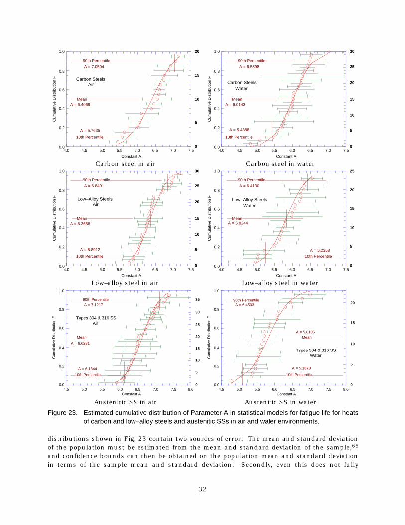
32

0.0

0.2

0.4

0.6

0.8

1.0

4.0 4.5 5.0 5.5 6.0 6.5 7.0 7.50

5

10

15

20C

umul

ativ

e D

istr

ibut

ion

F

Constant A

90th Percentile

10th Percentile

MeanA = 6.4069

A = 5.7635

A = 7.0504

Carbon SteelsAir

0.0

0.2

0.4

0.6

0.8

1.0

4.0 4.5 5.0 5.5 6.0 6.5 7.0 7.50

5

10

15

20

25

30

Cum

ulat

ive

Dis

trib

utio

n F

Constant A

90th Percentile

10th Percentile

MeanA = 6.0143

A = 5.4388

A = 6.5898

Carbon SteelsWater

Carbon steel in air Carbon steel in water

0.0

0.2

0.4

0.6

0.8

1.0

4.0 4.5 5.0 5.5 6.0 6.5 7.0 7.50

5

10

15

20

25

30

Cum

ulat

ive

Dis

trib

utio

n F

Constant A

90th Percentile

10th Percentile

MeanA = 6.3656

A = 5.8912

A = 6.8401

Low–Alloy SteelsAir

0.0

0.2

0.4

0.6

0.8

1.0

4.0 4.5 5.0 5.5 6.0 6.5 7.0 7.50

5

10

15

20

25

Cum

ulat

ive

Dis

trib

utio

n F

Constant A

90th Percentile

10th Percentile

MeanA = 5.8244

A = 5.2358

A = 6.4130

Low–Alloy SteelsWater

Low–alloy steel in air Low–alloy steel in water

0.0

0.2

0.4

0.6

0.8

1.0

4.5 5.0 5.5 6.0 6.5 7.0 7.5 8.00

5

10

15

20

25

30

35

Cum

ulat

ive

Dis

trib

utio

n F

Constant A

90th Percentile

10th Percentile

Mean

A = 6.6281

A = 6.1344

A = 7.1217

Types 304 & 316 SSAir

0.0

0.2

0.4

0.6

0.8

1.0

4.5 5.0 5.5 6.0 6.5 7.0 7.5 8.00

5

10

15

20

Cum

ulat

ive

Dis

trib

utio

n F

Constant A

90th Percentile

10th Percentile

MeanA = 5.8105

A = 5.1678

A = 6.4533

Types 304 & 316 SSWater

Austenitic SS in air Austenitic SS in water

Figure 23. Estimated cumulative distribution of Parameter A in statistical models for fatigue life for heatsof carbon and low–alloy steels and austenitic SSs in air and water environments.

distributions shown in Fig. 23 contain two sources of error. The mean and standard deviationof the population must be estimated from the mean and standard deviation of the sample,65

and confidence bounds can then be obtained on the population mean and standard deviationin terms of the sample mean and standard deviation. Secondly, even this does not fully

33

Table 3. Values of Parameter A in statistical model for carbon steels as a function ofconfidence level and percentage of population bounded

Confidence Percentage of Population Bounded (Percentile Distribution of A)Level 95 (5) 90 (10) 75 (25) 67 (33) 50 (50)

Air Environment50 5.930 6.019 6.212 6.278 6.40075 5.572 5.670 5.867 5.936 6.06590 5.251 5.356 5.555 5.627 5.76495 5.058 5.168 5.369 5.443 5.583

LWR Environments

50 5.300 5.444 5.675 5.767 5.94875 4.959 5.119 5.370 5.466 5.65290 4.652 4.836 5.095 5.195 5.38695 4.468 4.651 4.931 5.033 5.227

Table 4. Values of Parameter A in statistical model for low–alloy steels as a function ofconfidence level and percentage of population bounded


Air Environment50 5.912 6.000 6.180 6.242 6.37075 5.640 5.738 5.927 5.992 6.11990 5.395 5.503 5.700 5.768 5.89395 5.249 5.362 5.563 5.633 5.758

LWR Environments

50 5.049 5.210 5.496 5.623 5.82075 4.699 4.876 5.182 5.315 5.50890 4.383 4.575 4.898 5.037 5.22795 4.194 4.396 4.729 4.871 5.059

Table 5. Values of Parameter A in statistical model for austenitic stainless steels as a functionof confidence level and percentage of population bounded


Air Environment50 6.044 6.173 6.376 6.481 6.63175 5.721 5.878 6.102 6.217 6.37190 5.429 5.612 5.855 5.978 6.13795 5.255 5.453 5.707 5.836 5.997

LWR Environments

50 5.135 5.288 5.538 5.636 5.80575 4.755 4.928 5.193 5.297 5.46890 4.412 4.604 4.882 4.992 5.16495 4.208 4.410 4.696 4.809 4.983

address the uncertainty in the distribution, because of the large uncertainties in the samplevalues themselves, i.e., the “horizontal” uncertainty in the actual value of A for a heat ofmaterial, as indicated by the error bars in Fig. 23. A Monte Carlo analysis was used to addressboth sources of uncertainty. The results of the Monte Carlo analyses for various steels aresummarized in Tables 3–5 in terms of values for A that provide bounds for the portion of thepopulation and the confidence that is desired in the estimates of the bounds. Note that, withsmall samples, demanding too high a confidence level can lead to very conservative estimates of

34

Table 6. Margins on life for carbon steels corresponding to various confidence levels andpercentile values of Parameter A


Air Environment50 1.6 1.5 1.2 1.1 1.075 2.3 2.1 1.7 1.6 1.490 3.2 2.9 2.3 2.2 1.995 3.9 3.5 2.8 2.6 2.3

LWR Environments

50 2.0 1.8 1.4 1.3 1.075 2.9 2.4 1.9 1.7 1.490 3.9 3.3 2.5 2.3 1.995 4.7 3.9 3.0 2.7 2.2

Table 7. Margins on life for low–alloy steels corresponding to various confidence levels andpercentile values of Parameter A


Air Environment50 1.6 1.4 1.2 1.1 1.075 2.1 1.9 1.6 1.5 1.390 2.6 2.4 1.9 1.8 1.695 3.1 2.7 2.2 2.1 1.8

LWR Environments

50 2.2 1.8 1.4 1.2 1.075 3.1 2.6 1.9 1.7 1.490 4.2 3.5 2.5 2.2 1.895 5.1 4.2 3.0 2.6 2.1

Table 8. Margins on life for austenitic stainless steels corresponding to various confidencelevels and percentile values of Parameter A


Air Environment50 1.8 1.6 1.3 1.2 1.075 2.5 2.1 1.7 1.5 1.390 3.3 2.8 2.2 1.9 1.695 3.9 3.2 2.5 2.2 1.9

LWR Environments

50 2.0 1.7 1.3 1.2 1.075 2.9 2.4 1.9 1.7 1.490 4.0 3.3 2.5 2.3 1.995 5.0 4.1 3.0 2.7 2.3

the percentile values. Because the cumulative distributions in Fig. 23 do not properly accountfor all uncertainties, they should only be considered as a qualitative description of expectedvariation. Tables 3–5 should be used for quantitative estimates. For low–alloy steels, the 5thpercentile value of Parameter A at a 75% confidence level is 5.640 in air and 4.699 in LWRenvironments. From Fig. 23, the mean value of A for the sample is 6.366 and 5.824,respectively, in the two environments. Thus, for low–alloy steels, the 95/75 value of themargin to account for material variability and data scatter is 2.1 and 3.1 on life in air andwater environments, respectively. The corresponding margins in air and water environments,

35

respectively, are 2.3 and 2.9 for carbon steels, and 2.5 and 2.9 for SSs. Thus, average valuesof 2 and 3 on life in air and water environments, respectively, may be used to account foruncertainties due to material variability and data scatter. The estimated margins for thesesteels for various percentile and confidence levels are given in Tables 6–8. These margins areneeded to provide reasonable confidence that the resultant life will be greater than thatobserved for 95% of the materials of interest.

6.2 Size and Geometry

The effect of specimen size on the fatigue life has been investigated for smooth specimensof various diameters in the range of 2–60 mm.66–69 No intrinsic size effect has been observedfor smooth specimens tested in axial loading or plain bending. However, a size effect doesoccur in specimens tested in rotating bending; the fatigue endurance limit decreases by ª25%by increasing the specimen size from 2 to 16 mm but does not decrease further with largersizes.69 In addition, some effect of size and geometry has been observed on small–scale–vesseltests conducted at the Ecole Polytechnique in conjunction with the large–size–pressure–vesseltests carried out by the Southwest Research Institute.60 The tests at the Ecole Polytechniquewere conducted in room–temperature water on ª305–mm–inner–diameter, 19–mm–thick shellswith nozzles made of machined bar stock. The results indicate that the number of cyclesneeded to form a 3–mm–deep crack in a 19–mm–thick shell may be 30–50% lower than thatneeded for a small test specimen. Thus, a factor of ª1.4 on cycles and a factor of ª1.25 onstrain can be used to account for size and geometry.

6.3 Surface Finish

Fatigue life is sensitive to surface finish; cracks can initiate at surface irregularities thatare normal to the stress axis. The height, spacing, shape, and distribution of surfaceirregularities are important for crack initiation. The most common measure of roughness isaverage surface roughness Ra, which is a measure of the height of irregularities that arepresent. Investigations of the effects of surface roughness on the low–cycle fatigue of Type 304SS in air at 593°C indicate that fatigue life decreases as surface roughness increases.70,71 Theeffect of roughness on crack initiation Ni(R) is given by

Ni(Rq) = 1012 Rq–0.21, (25)

where the RMS value of surface roughness (Rq) is in micrometers. Studies indicate that an Raof 3 mm (or an Rq of 4 mm) represents the maximum surface roughness for drawing/extrusion,grinding, honing, and polishing processes and a mean value for the roughness range for millingor turning processes.72 For SSs, an Rq of 4 mm in Eq. 25 (Rq of a smooth polished specimen isª0.0075 mm) would decrease fatigue life by a factor of 3.7.70 A study of the effect of surfacefinish on the fatigue life of carbon steel in room–temperature air showed a factor of 2 decreasein life when Ra is increased from 0.3 to 5.3 mm.73 The experimental results from the presentstudy are consistent with Eq. 25. From Eq. 25, an Rq of 1.6 mm corresponds to a factor of 3.1decrease in fatigue life for the roughened specimen.

The experimental results suggest that factors of ª3 on cycles would account for effects ofsurface finish on the fatigue life of austenitic SSs in both air and water environments and forcarbon and low–alloy steels in air. A factor of 3 decrease in life corresponds to a factor of ª1.3on strain (Considering the factor of 20 on cycles to be equivalent to the factor of 2 on strain,

36

the factor applied on strain (KS) is obtained from the factor applied on cycles (KN) by using therelationship KS = (KN)0.2326). For carbon and low–alloy steels, the effect of surface finish is lowerin LWR environments; most likely, the moderate environmental effects (when any one thresholdcondition is not satisfied) are primarily due to surface roughness effects.

In earlier reports, Chopra and Shack15 and Chopra26 argued that the effects of surfacefinish may not be significant in LWR environments, because carbon and low–alloy steels andaustenitic SSs develop a rough corrosion scale. They further argued that the factor on life toaccount for the surface finish effect could be as low as 1.5 or perhaps eliminated completely inLWR environments. The results from the present study indicate that this argument is not validfor austenitic SSs, although the effect of surface roughness is small for carbon and low–alloysteels in LWR environments.

The decrease in fatigue life of both carbon and low–alloy steels and austenitic SSs iscaused primarily by the effect of the environment on the growth of microstructurally smallcracks and, to a lesser extent, on the growth of mechanically small cracks.43,44 The observedeffects of surface finish on the fatigue life of SSs and carbon and low–alloy steels in LWRenvironments appear to be consistent with the hypothesis that the mechanisms of the growthof microstructurally small cracks are different in austenitic SSs and carbon or low–alloy steels,although other explanations are also possible. The fact that the fatigue life of carbon andlow–alloy steels is unaffected by surface finish is consistent with the possibility of a mechanismlike slip/dissolution which is less dependent on the stress level. The reduction in life of SSs isconsistent with a hydrogen–enhanced crack growth mechanism, which seems more likely to beinfluenced by surface roughness.

6.4 Loading Sequence

The effects of variable amplitude loading of smooth specimens are well known.74–78 Thepresence in a loading sequence of a few cycles at high strain amplitude causes the fatigue lifeat smaller strain amplitude to be significantly lower than that at constant–amplitude loading.As discussed in Section 3.1, growth of mechanically small cracks can occur at strain levelsbelow the fatigue limit of the material. Fatigue life has conventionally been divided into twostages: initiation, expressed as the cycles required to form microcracks on the surface; andpropagation, expressed as cycles required to propagate the surface cracks to engineering size.During cyclic loading of smooth test specimens, surface cracks 10 mm or longer form quiteearly in life (i.e., <10% of life) at surface irregularities or discontinuities either already inexistence or produced by slip bands, grain boundaries, second–phase particles, etc.14,43,79–82

Consequently, fatigue life may be considered to be composed entirely of propagation of cracksfrom 10 to 3000 mm long.83

A schematic illustration of the two stages, i.e., initiation and propagation, of fatigue life isshown in Fig. 24. The initiation stage involves growth of microstructurally small cracks(MSCs), characterized by decelerating crack growth (Region AB in Fig. 24a). The propagationstage involves growth of mechanically small cracks, characterized by accelerating crack growth(Region BC in Fig. 24a). The growth of MSCs is very sensitive to microstructure.43,80 Fatiguecracks greater than the critical length of MSCs show little or no influence of microstructure,and are called mechanically small cracks, and they correspond to Stage II (tensile) cracks,which are characterized by striated crack growth, with a fracture surface normal to themaximum principal stress. Various criteria, summarized in Ref. 17, have been used to define

37

the crack length for transition from microstructurally to mechanically small crack; thetransition crack length is a function of applied stress and microstructure of the material;actual values may range from 150 to 250 mm.

At low stress levels (Ds1), the transition from MSC growth to accelerating crack growthdoes not occur. This circumstance represents the fatigue limit for the smooth specimen.Although cracks can form below the fatigue limit, they can grow to engineering size only atstresses greater than the fatigue limit. Note that the fatigue limit for a material is applicableonly for constant loading conditions. Under variable loading conditions encountered duringservice of power plants, cracks created by growth of MSCs at high stresses (Ds3) to lengthslarger than the transition crack length can increase at stress levels below the fatigue limit(Ds1).

Studies on fatigue damage in Type 304 SS under complex loading histories78 indicatethat the loading sequence of decreasing strain levels (i.e., high strain level followed by lowstrain level) is more damaging than that of increasing strain levels. The fatigue life of the steeldecreased by a factor of 2–4 under a decreasing–strain sequence. In another study, the fatiguelimit of medium carbon steels was lowered even after low–stress high–cycle fatigue; the higherthe stress, the greater the decrease in fatigue threshold.84 In general, the mean fatigue e–Ncurves are lowered to account for damaging cycles that occur below the constant–amplitudefatigue limit of the material.85 A factor of 1.5–2.5 on cycles and 1.3–1.6 on strain may be usedto incorporate the effects of load histories on fatigue life.

6.5 Moderate or Acceptable Environmental Effects

A working group of the PVRC has been compiling and evaluating data on the effects ofLWR coolant environments on the fatigue life of pressure boundary materials.31 One of thetasks in the PVRC activity was to define a set of values for material, loading, and environmentalvariables that lead to moderate or acceptable effects of environment on fatigue life. A factor of4 on the ASME mean life was chosen as a working definition of “moderate” or “acceptable”effects of environment, i.e., up to a factor of 4 decrease in fatigue life due to the environment isconsidered acceptable and does not require further fatigue evaluation.31 The basis for this

0 0.2 0.4 0.6 0.8 1

Cra

ck L

engt

h

Life Fraction

Microstructurally Small Crack (MSC)(Stage–I Shear Crack)

Mechanically Small Crack(Stage II Tensile Crack)

A

B

C

Ds2

Ds1

Ds 2 > Ds1

Cra

ck V

eloc

ity (

da/d

N)

Crack Length

MSC

LEFM

D s 1

Non–PropagatingCracks

Short Cracks

D s3

D s 2

D s 3 > D s 2 > D s1

D s1

(a) (b)Figure 24. Schematic illustration of (a) growth of short cracks in smooth specimens as a

function of fatigue life fraction and (b) crack velocity as a function of crack length.LEFM = linear elastic fracture mechanics.

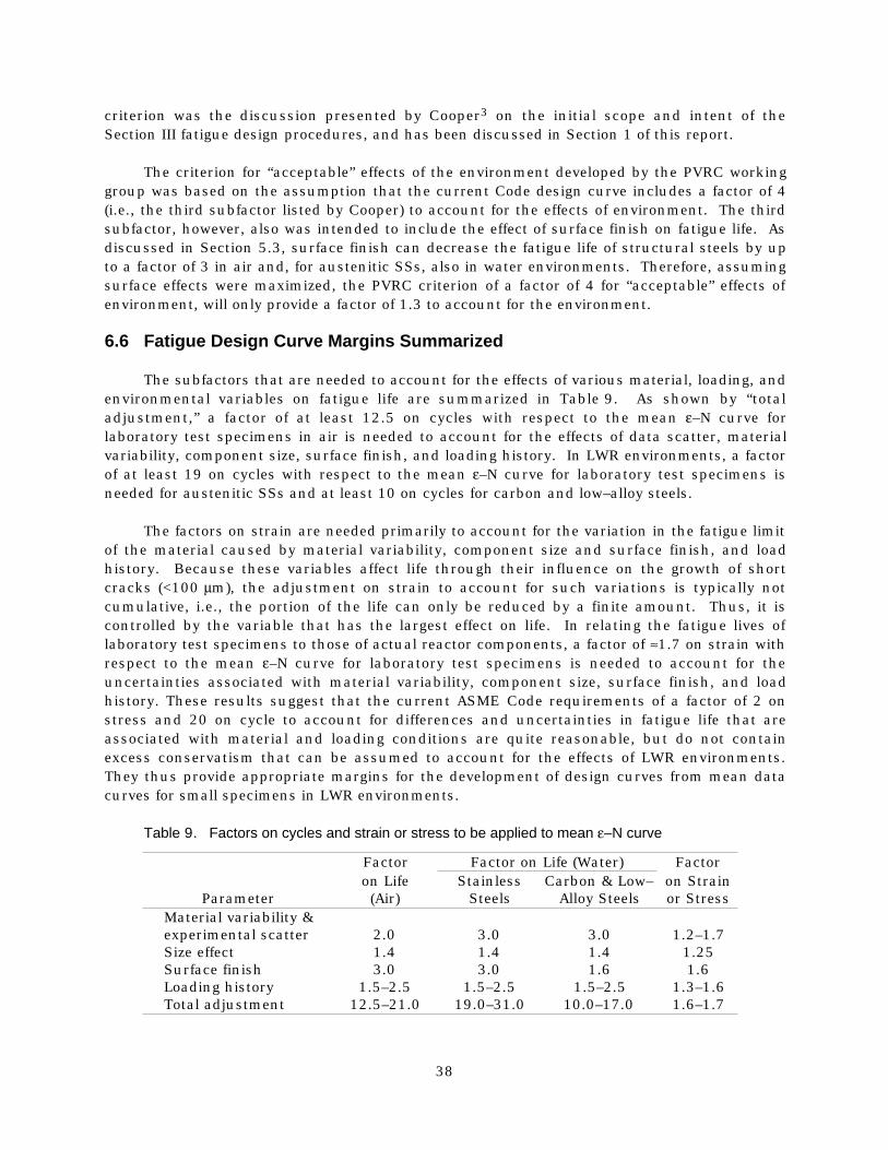
38

criterion was the discussion presented by Cooper3 on the initial scope and intent of theSection III fatigue design procedures, and has been discussed in Section 1 of this report.

The criterion for “acceptable” effects of the environment developed by the PVRC workinggroup was based on the assumption that the current Code design curve includes a factor of 4(i.e., the third subfactor listed by Cooper) to account for the effects of environment. The thirdsubfactor, however, also was intended to include the effect of surface finish on fatigue life. Asdiscussed in Section 5.3, surface finish can decrease the fatigue life of structural steels by upto a factor of 3 in air and, for austenitic SSs, also in water environments. Therefore, assumingsurface effects were maximized, the PVRC criterion of a factor of 4 for “acceptable” effects ofenvironment, will only provide a factor of 1.3 to account for the environment.

6.6 Fatigue Design Curve Margins Summarized

The subfactors that are needed to account for the effects of various material, loading, andenvironmental variables on fatigue life are summarized in Table 9. As shown by “totaladjustment,” a factor of at least 12.5 on cycles with respect to the mean e–N curve forlaboratory test specimens in air is needed to account for the effects of data scatter, materialvariability, component size, surface finish, and loading history. In LWR environments, a factorof at least 19 on cycles with respect to the mean e–N curve for laboratory test specimens isneeded for austenitic SSs and at least 10 on cycles for carbon and low–alloy steels.

The factors on strain are needed primarily to account for the variation in the fatigue limitof the material caused by material variability, component size and surface finish, and loadhistory. Because these variables affect life through their influence on the growth of shortcracks (<100 mm), the adjustment on strain to account for such variations is typically notcumulative, i.e., the portion of the life can only be reduced by a finite amount. Thus, it iscontrolled by the variable that has the largest effect on life. In relating the fatigue lives oflaboratory test specimens to those of actual reactor components, a factor of ª1.7 on strain withrespect to the mean e–N curve for laboratory test specimens is needed to account for theuncertainties associated with material variability, component size, surface finish, and loadhistory. These results suggest that the current ASME Code requirements of a factor of 2 onstress and 20 on cycle to account for differences and uncertainties in fatigue life that areassociated with material and loading conditions are quite reasonable, but do not containexcess conservatism that can be assumed to account for the effects of LWR environments.They thus provide appropriate margins for the development of design curves from mean datacurves for small specimens in LWR environments.

Table 9. Factors on cycles and strain or stress to be applied to mean e–N curve

Factor Factor on Life (Water) Factor

Parameteron Life(Air)

StainlessSteels

Carbon & Low–Alloy Steels

on Strainor Stress

Material variability &experimental scatter 2.0 3.0 3.0 1.2–1.7Size effect 1.4 1.4 1.4 1.25Surface finish 3.0 3.0 1.6 1.6Loading history 1.5–2.5 1.5–2.5 1.5–2.5 1.3–1.6Total adjustment 12.5–21.0 19.0–31.0 10.0–17.0 1.6–1.7

39

7 Summary

The existing fatigue e–N data for carbon and low–alloy steels and wrought and castaustenitic SSs have been evaluated to define the effects of key material, loading, andenvironmental parameters on the fatigue lives of these steels. The fatigue lives of carbon andlow–alloy steels and austenitic SSs are decreased in LWR environments; the magnitude of thereduction depends on temperature, strain rate, DO level in water, and, for carbon andlow–alloy steels, the S content of the steel. For all steels, environmental effects on fatigue lifeare significant only when critical parameters (temperature, strain rate, DO level, and strainamplitude) meet certain threshold values. Environmental effects are moderate, e.g., less than afactor of 2 decrease in life, when any one of the threshold conditions is not satisfied. Thethreshold values of the critical parameters and the effects of other parameters (such as waterconductivity, water flow rate, and material heat treatment) on the fatigue life of the steels aresummarized.

Experimental data are presented on the effects of surface roughness on the fatigue life ofcarbon and low–alloy steels and austenitic SSs in air and LWR environments. Tests wereconducted on specimens that were intentionally roughened under controlled conditions to anRMS surface roughness of 1.6 mm. For austenitic SSs, the fatigue life of roughened specimensis a factor of ª3 lower than that of the smooth specimens in both air and low–DO water. Inhigh–DO water, fatigue lives are comparable for smooth and roughened specimens. For carbonand low–alloy steels, the fatigue life of roughened specimens is lower than that of smoothspecimens in air but, in high–DO water, it is the same. In low–DO water, the fatigue life of theroughened specimens is slightly lower than that of smooth specimens. Because environmentaleffects on carbon and low–alloy steels are moderate in low–DO water, surface roughness isexpected to influence fatigue life.

Statistical models are presented for estimating the fatigue life of carbon and low–alloysteels and wrought and cast austenitic SSs as a function of material, loading, andenvironmental parameters. Functional form and bounding values of these parameters arebased on experimental observations and data trends. The models are recommended forpredicted fatigue lives of £106 cycles.

Two approaches are presented for incorporating the effects of LWR environments intoASME Section III fatigue evaluations. Both approaches are based on the best–fit curves to theexperimental fatigue e–N data in LWR environments. In the first approach, environmentallyadjusted fatigue design curves have been developed by adjusting the best–fit experimentalcurve for the effect of mean stress and by setting margins of 20 on cycles and 2 on strain toaccount for uncertainties in life associated with material and loading conditions. These curvesprovide allowable cycles for fatigue crack initiation in LWR coolant environments. The secondapproach considers the effects of reactor coolant environments on fatigue life in terms of anenvironmental correction factor Fen, which is the ratio of fatigue life in air at room temperatureto that in water under reactor operating conditions. To incorporate environmental effects intothe ASME Code fatigue evaluations, a fatigue usage factor for a specific load set, based on thecurrent Code design curves, is multiplied by the correction factor.

Data available in the literature have been reviewed to evaluate the conservatism in theexisting ASME Code fatigue evaluations. Much of the conservatism in these evaluations arises

40

from current design procedures, e.g., stress analysis rules and cycle counting. However, theASME Code permits alternative approaches, such as finite–element analyses, fatiguemonitoring, and improved Ke factors, that can significantly decrease the conservatism in thecurrent fatigue evaluation procedures.

Because of material variability, data scatter, and component size and surface, the fatiguelife of actual components differ from that of laboratory test specimens under a similar loadinghistory, and the mean e–N curves for laboratory test specimens must be adjusted to obtaindesign curves for components. These design margins are another source of possibleconservatism. The factors of 2 on stress and 20 on cycles used in the Code were intended tocover the effects of variables that can influence fatigue life but were not investigated in thetests that provided the data for the curves. Although these factors were intended to besomewhat conservative, they should not be considered safety margins because they wereintended to account for variables that are known to affect fatigue life. Data available in theliterature have been reviewed to evaluate the margins on cycles and stress that are needed toaccount for the differences and uncertainties. In air, a factor of at least 12.5 on cycles withrespect to the mean e–N curve for laboratory test specimens is needed to account for the effectsof data scatter and material variability, component size, surface finish, and loading sequence.In LWR environments, a factor of at least 19 on cycles with respect to the mean e–N curve forlaboratory test specimens is needed for austenitic SSs and at least 10 on cycles for carbon andlow–alloy steels. Also, in air and LWR environments, a factor of 1.7 on stress is needed toaccount for the various differences and uncertainties. The results indicate that the currentASME Code requirements of a factor of 2 on stress and 20 on cycles are quite reasonable, butdo not contain excess conservatism that can be assumed to account for the effects of LWRenvironments. They thus provide appropriate design margins for the development of designcurves from mean data curves for small specimens in LWR environments.

41

References

1. B. F. Langer, “Design of Pressure Vessels for Low–Cycle Fatigue,” ASME J. Basic Eng. 84,389–402 (1962).

2. Criteria of the ASME Boiler and Pressure Vessel Code for Design by Analysis inSections III and VIII, Division 2, The American Society of Mechanical Engineers, New York(1969).

3. W. E. Cooper, “The Initial Scope and Intent of the Section III Fatigue Design Procedure,”in Welding Research Council, Inc., Technical Information from Workshop on Cyclic Lifeand Environmental Effects in Nuclear Applications, Clearwater, Florida, January 20–21,1992.

4. S. Ranganath, J. N. Kass, and J. D. Heald, “Fatigue Behavior of Carbon SteelComponents in High–Temperature Water Environments,” BWR Environmental CrackingMargins for Carbon Steel Piping, EPRI NP–2406, Electric Power Research Institute,Palo Alto, CA, Appendix 3 (1982).

5. M. Higuchi and K. Iida, “Fatigue Strength Correction Factors for Carbon and Low–AlloySteels in Oxygen–Containing High–Temperature Water,” Nucl. Eng. Des. 129, 293–306(1991).

6. N. Nagata, S. Sato, and Y. Katada, “Low–Cycle Fatigue Behavior of Pressure Vessel Steelsin High–Temperature Pressurized Water,” ISIJ Intl. 31 (1), 106–114 (1991).

7. Y. Katada, N. Nagata, and S. Sato, “Effect of Dissolved Oxygen Concentration on FatigueCrack Growth Behavior of A533 B Steel in High–Temperature Water,” ISIJ Intl. 33 (8),877–883 (1993).

8. H. Kanasaki, M. Hayashi, K. Iida, and Y. Asada, “Effects of Temperature Change onFatigue Life of Carbon Steel in High Temperature Water,” in Fatigue and Crack Growth:Environmental Effects, Modeling Studies, and Design Considerations, PVP Vol. 306,S. Yukawa, ed., American Society of Mechanical Engineers, New York, pp. 117–122(1995).

9. G. Nakao, H. Kanasaki, M. Higuchi, K. Iida, and Y. Asada, “Effects of Temperature andDissolved Oxygen Content on Fatigue Life of Carbon and Low–Alloy Steels in LWR WaterEnvironment,” in Fatigue and Crack Growth: Environmental Effects, Modeling Studies,and Design Considerations, PVP Vol. 306, S. Yukawa, ed., American Society ofMechanical Engineers, New York, pp. 123–128 (1995).

10. M. Higuchi, K. Iida, and Y. Asada, “Effects of Strain Rate Change on Fatigue Life ofCarbon Steel in High–Temperature Water,” in Effects of the Environment on the Initiationof Crack Growth, ASTM STP 1298, W. A. Van Der Sluys, R. S. Piascik, andR. Zawierucha, eds., American Society for Testing and Materials, Philadelphia, pp.216–231 (1997).

42

11. K. Iida, T. Bannai, M. Higuchi, K. Tsutsumi, and K. Sakaguchi, “Comparison of JapaneseMITI Guideline and Other Methods for Evaluation of Environmental Fatigue LifeReduction,” in Pressure Vessel and Piping Codes and Standards, PVP Vol. 419, M. D.Rana, ed., American Society of Mechanical Engineers, New York, pp. 73–82 (2001).

12. O. K. Chopra and W. J. Shack, “Evaluation of Effects of LWR Coolant Environments onFatigue Life of Carbon and Low–Alloy Steels,” in Effects of the Environment on theInitiation of Crack Growth, ASTM STP 1298, W. A. Van Der Sluys, R. S. Piascik, andR. Zawierucha, eds., American Society for Testing and Materials, Philadelphia,pp. 247–266 (1997).

13. O. K. Chopra and W. J. Shack, “Low–Cycle Fatigue of Piping and Pressure Vessel Steels inLWR Environments,” Nucl. Eng. Des. 184, 49–76 (1998).

14. O. K. Chopra and W. J. Shack, “Effects of LWR Coolant Environments on Fatigue DesignCurves of Carbon and Low–Alloy Steels,” NUREG/CR–6583, ANL–97/18 (March 1998).

15. O. K. Chopra and W. J. Shack, “Overview of Fatigue Crack Initiation in Carbon andLow–Alloy Steels in Light Water Reactor Environments,” J. Pressure Vessel Technol. 121,49–60 (1999).

16. O. K. Chopra and J. Muscara, “Effects of Light Water Reactor Coolant Environments onFatigue Crack Initiation in Piping and Pressure Vessel Steels,” in Proc. 8th Intl.Conference on Nuclear Engineering, 2.08 LWR Materials Issue, Paper 8300, AmericanSociety of Mechanical Engineers, New York (2000).

17. O. K. Chopra and W. J. Shack, “Environmental Effects on Fatigue Crack Initiation inPiping and Pressure Vessel Steels,” NUREG/CR–6717, ANL–00/27 (May 2001).

18. M. Fujiwara, T. Endo, and H. Kanasaki, “Strain Rate Effects on the Low–Cycle FatigueStrength of 304 Stainless Steel in High–Temperature Water Environment; Fatigue Life:Analysis and Prediction,” in Proc. Intl. Conf. and Exposition on Fatigue, CorrosionCracking, Fracture Mechanics, and Failure Analysis, ASM, Metals Park, OH, pp. 309–313(1986).

19. M. Higuchi and K. Iida, “Reduction in Low–Cycle Fatigue Life of Austenitic StainlessSteels in High–Temperature Water,” in Pressure Vessel and Piping Codes and Standards,PVP Vol. 353, D. P. Jones, B. R. Newton, W. J. O'Donnell, R. Vecchio, G. A. Antaki,D. Bhavani, N. G. Cofie, and G. L. Hollinger, eds., American Society of MechanicalEngineers, New York, pp. 79–86 (1997).

20. H. Kanasaki, R. Umehara, H. Mizuta, and T. Suyama, “Effect of Strain Rate andTemperature Change on the Fatigue Life of Stainless Steel in PWR Primary Water,” Trans.14th Intl. Conf. on Structural Mechanics in Reactor Technology (SMiRT 14), Lyon,France, pp. 485–493 (1997).

21. H. Kanasaki, R. Umehara, H. Mizuta, and T. Suyama, “Fatigue Lives of Stainless Steels inPWR Primary Water,” Trans. 14th Intl. Conf. on Structural Mechanics in ReactorTechnology (SMiRT 14), Lyon, France, pp. 473–483 (1997).

43

22. K. Tsutsumi, H. Kanasaki, T. Umakoshi, T. Nakamura, S. Urata, H. Mizuta, andS. Nomoto, “Fatigue Life Reduction in PWR Water Environment for Stainless Steels,” inAssessment Methodologies for Preventing Failure: Service Experience and EnvironmentalConsiderations, PVP Vol. 410-2, R. Mohan, ed., American Society of MechanicalEngineers, New York, pp. 23–34 (2000).

23. K. Tsutsumi, T. Dodo, H. Kanasaki, S. Nomoto, Y. Minami, and T. Nakamura, “FatigueBehavior of Stainless Steel under Conditions of Changing Strain Rate in PWR PrimaryWater,” in Pressure Vessel and Piping Codes and Standards, PVP Vol. 419, M. D. Rana,ed., American Society of Mechanical Engineers, New York, pp. 135–141 (2001).

24. O. K. Chopra and D. J. Gavenda, “Effects of LWR Coolant Environments on Fatigue Livesof Austenitic Stainless Steels,” J. Pressure Vessel Technol. 120, 116–121 (1998).

25. O. K. Chopra and J. L. Smith, “Estimation of Fatigue Strain–Life Curves for AusteniticStainless Steels in Light Water Reactor Environments,” in Fatigue, EnvironmentalFactors, and New Materials, PVP Vol. 374, H. S. Mehta, R. W. Swindeman, J. A. Todd,S. Yukawa, M. Zako, W. H. Bamford, M. Higuchi, E. Jones, H. Nickel, and S. Rahman,eds., American Society of Mechanical Engineers, New York, pp. 249–259 (1998).

26. O. K. Chopra, “Effects of LWR Coolant Environments on Fatigue Design Curves ofAustenitic Stainless Steels,” NUREG/CR–5704, ANL–98/31 (1999).

27. O. K. Chopra, “Mechanism and Estimation of Fatigue Crack Initiation in AusteniticStainless Steels in LWR Environments,” NUREG/CR–6787, ANL–01/25 (2002).

28. O. K. Chopra, “Development of Fatigue Design Curve for Austenitic Stainless Steels inLWR Environments: A Review,” in Pressure Vessel and Piping Codes and Standards -2002, PVP Vol. 439, R. D. Rana, ed., American Society of Mechanical Engineers,New York, pp. 119–132 (2002).

29. S. Majumdar, O. K. Chopra, and W. J. Shack, “Interim Fatigue Design Curves for Carbon,Low–Alloy, and Austenitic Stainless Steels in LWR Environments,” NUREG/CR–5999,ANL–93/3 (1993).

30. J. Keisler, O. K. Chopra, and W. J. Shack, “Fatigue Strain–Life Behavior of Carbon andLow–Alloy Steels, Austenitic Stainless Steels, and Alloy 600 in LWR Environments,”NUREG/CR–6335, ANL–95/15 (1995).

31. W. A. Van Der Sluys and S. Yukawa, “Status of PVRC Evaluation of LWR CoolantEnvironmental Effects on the S–N Fatigue Properties of Pressure Boundary Materials,” inFatigue and Crack Growth: Environmental Effects, Modeling Studies, and DesignConsiderations, PVP Vol. 306, S. Yukawa, ed., American Society of Mechanical Engineers,New York, pp. 47–58 (1995).

32. J. L. Smith, O. K. Chopra, and W. J. Shack, “Effect of Water Chemistry on the FatigueLife of Austenitic Stainless Steels in LWR Environments,” in Environmentally AssistedCracking in Light Water Reactors, Semiannual Report, January 1999–June 1999,NUREG/CR–4667, Vol. 28, ANL–00/7, pp. 13–27 (July 2000).

44

33. D. A. Hale, S. A. Wilson, E. Kiss, and A. J. Gianuzzi, “Low Cycle Fatigue Evaluation ofPrimary Piping Materials in a BWR Environment,” GEAP–20244, U.S. Nuclear RegulatoryCommission (1977).

34. D. A. Hale, S. A. Wilson, J. N. Kass, and E. Kiss, “Low Cycle Fatigue Behavior ofCommercial Piping Materials in a BWR Environment,” J. Eng. Mater. Technol. 103, 15–25(1981).

35. S. Ranganath, J. N. Kass, and J. D. Heald, “Fatigue Behavior of Carbon SteelComponents in High–Temperature Water Environments,” in Low–Cycle Fatigue and LifePrediction, ASTM STP 770, C. Amzallag, B. N. Leis, and P. Rabbe, eds., American Societyfor Testing and Materials, Philadelphia, pp. 436–459 (1982).

36. J. B. Terrell, “Fatigue Life Characterization of Smooth and Notched Piping SteelSpecimens in 288°C Air Environments,” NUREG/CR–5013, EM–2232 MaterialsEngineering Associates, Inc., Lanham, MD (1988).

37. J. B. Terrell, “Fatigue Strength of Smooth and Notched Specimens of ASME SA 106–BSteel in PWR Environments,” NUREG/CR–5136, MEA–2289, Materials EngineeringAssociates, Inc., Lanham, MD (1988).

38. C. E. Jaske and W. J. O'Donnell, “Fatigue Design Criteria for Pressure Vessel Alloys,”Trans. ASME J. Pressure Vessel Technol. 99, 584–592 (1977).

39. J. B. Conway, R. H. Stentz, and J. T. Berling, “Fatigue, Tensile, and Relaxation Behaviorof Stainless Steels,” TID–26135, U.S. Atomic Energy Commission, Washington, DC(1975).

40. D. L. Keller, “Progress on LMFBR Cladding, Structural, and Component Materials Studiesduring July, 1971 through June, 1972, Final Report,” Task 32, Battelle–ColumbusLaboratories, BMI–1928 (1977).

41. M. Hayashi, “Thermal Fatigue Strength of Type 304 Stainless Steel in Simulated BWREnvironment,” Nucl. Eng. Des. 184, 135–144 (1998).

42. M. Hayashi, K. Enomoto, T. Saito, and T. Miyagawa, “Development of Thermal FatigueTesting with BWR Water Environment and Thermal Fatigue Strength of AusteniticStainless Steels,” Nucl. Eng. Des. 184, 113–122 (1998).

43. D. J. Gavenda, P. R. Luebbers, and O. K. Chopra, “Crack Initiation and Crack GrowthBehavior of Carbon and Low–Alloy Steels,” in Fatigue and Fracture 1, Vol. 350,S. Rahman, K. K. Yoon, S. Bhandari, R. Warke, and J. M. Bloom, eds., American Societyof Mechanical Engineers, New York, pp. 243–255 (1997).

44. O. K. Chopra, “Mechanism of Fatigue Crack Initiation in Austenitic Stainless Steels inLWR Environments,” in Pressure Vessel and Piping Codes and Standards - 2002, PVPVol. 439, R. D. Rana, ed., American Society of Mechanical Engineers, New York,pp. 133–142 (2002).

45

45. T. T. Pleune and O. K. Chopra, “Artificial Neural Networks and Effects of LoadingConditions on Fatigue Life of Carbon and Low–Alloy Steels,” in Fatigue and Fracture 1,Vol. 350, S. Rahman, K. K. Yoon, S. Bhandari, R. Warke, and J. M. Bloom, eds.,American Society of Mechanical Engineers, New York, pp. 413–423 (1997).

46. G. L. Wire and Y. Y. Li, “Initiation of Environmentally–Assisted Cracking in Low–AlloySteels,” in Fatigue and Fracture Volume 1, PVP Vol. 323, H. S. Mehta, ed., AmericanSociety of Mechanical Engineers, New York, pp. 269–289 (1996).

47. J. Hickling, “Strain–Induced Corrosion Cracking of Low–Alloy Reactor Pressure VesselSteels under BWR Conditions,” in Proc. of the Tenth Intl. Symp. on EnvironmentalDegradation of Materials in Nuclear Power Systems-Water Reactors, F. P. Ford, S. M.Bruemmer, and G. S. Was, eds., The Minerals, Metals, and Materials Society, Warrendale,PA, CD-ROM, Paper 0156 (2001).

48. H. D. Solomon, R. E. DeLair, and A. D. Unruh, “Crack Initiation in Low–Alloy Steel inHigh–Temperature Water,” in Effects of the Environment on the Initiation of CrackGrowth, ASTM STP 1298, W. A. Van Der Sluys, R. S. Piascik, and R. Zawierucha, eds.,American Society for Testing and Materials, Philadelphia, pp. 135–149 (1997).

49. H. D. Solomon, R. E. DeLair, and E. Tolksdorf, “LCF Crack Initiation in WB36 in HighTemperature Water,” in Proc. of the Ninth Intl. Symp. on Environmental Degradation ofMaterials in Nuclear Power Systems-Water Reactors, F. P. Ford, S. M. Bruemmer, andG. S. Was, eds., The Minerals, Metals, and Materials Society, Warrendale, PA, pp. 865-872 (1999).

50. A. Hirano, M. Yamamoto, K. Sakaguchi, K. Iida, and T. Shoji, “Effects of Water Flow Rateon Fatigue Life of Carbon Steel in High–Temperature Pure Water Environment,” inAssessment Methodologies for Predicting Failure: Service Experience and EnvironmentalConsiderations, PVP Vol. 410–2, R. Mohan, ed., American Society of MechanicalEngineers, New York, pp. 13–18 (2000).

51. A. Hirano, M. Yamamoto, K. Sakaguchi, T. Shoji, and K. Iida, “Effects of Water Flow Rateon Fatigue Life of Ferritic and Austenitic Steels in Simulated LWR Environment,” inPressure Vessel and Piping Codes and Standards - 2002, PVP Vol. 439, R. D. Rana, ed.,American Society of Mechanical Engineers, New York, pp. 143–150 (2002).

52. E. Lenz, N. Wieling, and H. Muenster, “Influence of Variation of Flow Rates andTemperature on the Cyclic Crack Growth Rate under BWR Conditions,” in EnvironmentalDegradation of Materials in Nuclear Power Systems – Water Reactors, The MetallurgicalSociety, Warrendale, PA (1988).

53. C. Amzallag, P. Rabbe, G. Gallet, H. –P. Lieurade, “Influence des Conditions deSollicitation Sur le Comportement en Fatigue Oligocyclique D'aciers InoxydablesAusténitiques,” Memoires Scientifiques Revue Metallurgie Mars, pp. 161–173 (1978).

54. H. S. Mehta and S. R. Gosselin, “Environmental Factor Approach to Account for WaterEffects in Pressure Vessel and Piping Fatigue Evaluations,” Nucl. Eng. Des. 181, 175–197(1998).

46

55. H. S. Mehta, “An Update on the EPRI/GE Environmental Fatigue Evaluation Methodologyand its Applications,” in Probabilistic and Environmental Aspects of Fracture andFatigues, PVP Vol. 386, S. Rahman, ed., American Society of Mechanical Engineers,New York, pp. 183–193 (1999).

56. G. L. Wire, T. R. Leax, and J. T. Kandra, “Mean Stress and Environmental Effects onFatigue in Type 304 Stainless Steel,” in Probabilistic and Environmental Aspects ofFracture and Fatigues, PVP Vol. 386, S. Rahman, ed., American Society of MechanicalEngineers, New York, pp. 213–228 (1999).

57. M. E. Mayfield, E. C. Rodabaugh, and R. J. Eiber, “A Comparison of Fatigue Test Data onPiping with the ASME Code Fatigue Evaluation Procedure,” ASME Paper 79–PVP–92,American Society of Mechanical Engineers, New York (1979).

58. J. D. Heald and E. Kiss, “Low Cycle Fatigue of Nuclear Pipe Components,” J. PressureVessel Technol. 74, PVP–5, 1–6 (1974).

59. A. F. Deardorff and J. K. Smith, “Evaluation of Conservatisms and Environmental Effectsin ASME Code, Section III, Class 1 Fatigue Analysis,” SAND94–0187, prepared byStructural Integrity Associates, San Jose, CA, under contract to Sandia NationalLaboratories, Albuquerque, NM (1994).

60. L. F. Kooistra, E. A. Lange, and A. G. Pickett, “Full–Size Pressure Vessel Testing and ItsApplication to Design,” J. Eng. Power 86, 419–428 (1964).

61. P. M. Scott and G. M. Wilkowski, “A Comparison of Recent Full–Scale Component FatigueData with the ASME Section III Fatigue Design Curves,” in Fatigue and Crack Growth:Environmental Effects, Modeling Studies, and Design Considerations, PVP Vol. 306,S. Yukawa, ed., American Society of Mechanical Engineers, New York, pp. 129–138(1995).

62. J. Hechmer, “Evaluation Methods for Fatigue - A PVRC Project,” in Fatigue,Environmental Factors, and New Materials, PVP Vol. 374, H. S. Mehta, R. W. Swindeman,J. A. Todd, S. Yukawa, M. Zako, W. H. Bamford, M. Higuchi, E. Jones, H. Nickel, andS. Rahman, eds., American Society of Mechanical Engineers, New York, pp. 191–199(1998).

63. L. G. Johnson, “The Median Ranks of Sample Values in Their Population with anApplication to Certain Fatigue Studies,” Ind. Math. 2, 1–9 (1951).

64. C. Lipson and N. J. Sheth, Statistical Design and Analysis of Engineering Experiments,McGraw Hill, New York (1973).

65. J. Beck and K. Arnold, Parameter Estimation in Engineering and Science, J. Wiley,New York (1977).

66. R. E. Peterson, “Fatigue Tests of Small Specimens with Particular Reference to SizeEffect,” Trans. Amer. Soc. Steel Testing 18, 1041–1053 (1930).

47

67. D. Morkovin and H. F. Moore, “Third Progress Report on the Effect of Size of Specimen onFatigue Strength of Three Types of Steel,” Proc. Amer. Soc. Test. Mater. 44, 137–158(1944).

68. C. E. Philips and R. B. Heywood, “The Size Effect in Fatigue of Plain and Notched SteelSpecimens Loaded under Reversed Direct Stress,” Proc. Inst. Mech. Eng. 165, 113–124(1951).

69. C. Massonnet, “The Effect of Size, Shape, and Grain Size on the Fatigue Strength ofMedium Carbon Steel,” Proc. Amer. Soc. Test. Mater. 56, 954–978 (1956).

70. P. S. Maiya and D. E. Busch, “Effect of Surface Roughness on Low–Cycle FatigueBehavior of Type 304 Stainless Steel,” Met. Trans. 6A, 1761–1766 (1975).

71. P. S. Maiya, “Effect of Surface Roughness and Strain Range on Low–Cycle FatigueBehavior of Type 304 Stainless Steel,” Scripta Metall. 9, 1277–1282 (1975).

72. K. J. Stout, “Surface Roughness – Measurement, Interpretation, and Significance ofData,” Mater. Eng. 2, 287–295 (1981).

73. K. Iida, “A Study of Surface Finish Effect Factor in ASME B & PV Code Section III,” inPressure Vessel Technology, Vol. 2, L. Cengdian and R. W. Nichols, eds., Pergamon Press,New York, pp. 727–734 (1989).

74. M. A. Pompetzki, T. H. Topper, and D. L. DuQuesnay, “The Effect of CompressiveUnderloads and Tensile Overloads on Fatigue Damage Accumulation in SAE 1045 Steel,”Int. J. Fatigue 12 (3), 207–213 (1990).

75. A. Conle and T. H. Topper, “Evaluation of Small Cycle Omission Criteria for Shortening ofFatigue Service Histories,” Int. J. Fatigue 1, 23–28 (1979).

76. A. Conle and T. H. Topper, “Overstrain Effects During Variable Amplitude Service HistoryTesting,” Int. J. Fatigue 2, 130–136 (1980).

77. Li Nian and Du Bai–Ping, “Effect of Monotonic and Cyclic Prestrain on the FatigueThreshold in Medium–Carbon Steels,” Int. J. Fatigue 14 (1), 41–44 (1992).

78. M. J. Manjoine, “Fatigue Damage Models for Annealed Type 304 Stainless Steel underComplex Strain Histories,” Trans. 6th Intl. Conf. on Structural Mechanics in ReactorTechnology (SMiRT), Vol. L, 8/1, North–Holland Publishing Co., pp. 1–13 (1981).

79. K. J Miller, “Initiation and Growth Rates of Short Fatigue Cracks,” Fundamentals ofDeformation and Fracture, Eshelby Memorial Symposium, Cambridge University Press,Cambridge, U.K., pp. 477–500 (1985).

80. K. Tokaji, T. Ogawa, and S. Osaka, “The Growth of Microstructurally Small FatigueCracks in a Ferrite–Pearlite Steel,” Fatigue Fract. Eng. Mater. Struct. 11, 311–342 (1988).

81. K. Obrtlik, J. Polák, M. Hájek, and A. Vasek, “Short Fatigue Crack Behaviour in 316LStainless Steel,” Intl. J. Fatigue 19, 471–475 (1997).

48

82. S. G. Sundara Raman, D. Argence, and A. Pineau, “High–Temperature Short FatigueCrack Behaviour in a Stainless Steel,” Fatigue Fract. Eng. Mater. Struct. 20, 1015–1031(1997).

83. K. J. Miller, “Damage in Fatigue: A New Outlook,” in International Pressure Vessels andPiping Codes and Standards: Volume 1 – Current Applications, PVP Vol. 313–1, K. R. Raoand Y. Asada, eds., American Society of Mechanical Engineers, New York, pp. 191–192(1995).

84. Li Nian and Du Bai–Ping, “The Effect of Low–Stress High–Cycle Fatigue on theMicrostructure and Fatigue Threshold of a 40Cr Steel,” Int. J. Fatigue 17 (1), 43–48(1995).

85. E. Haibach and D. Schutz, “Fatigue Life Evaluation with Particular Attention to LocalStrain and Stress Time Histories,” Proc. Inst. Mech. Eng. (1974).

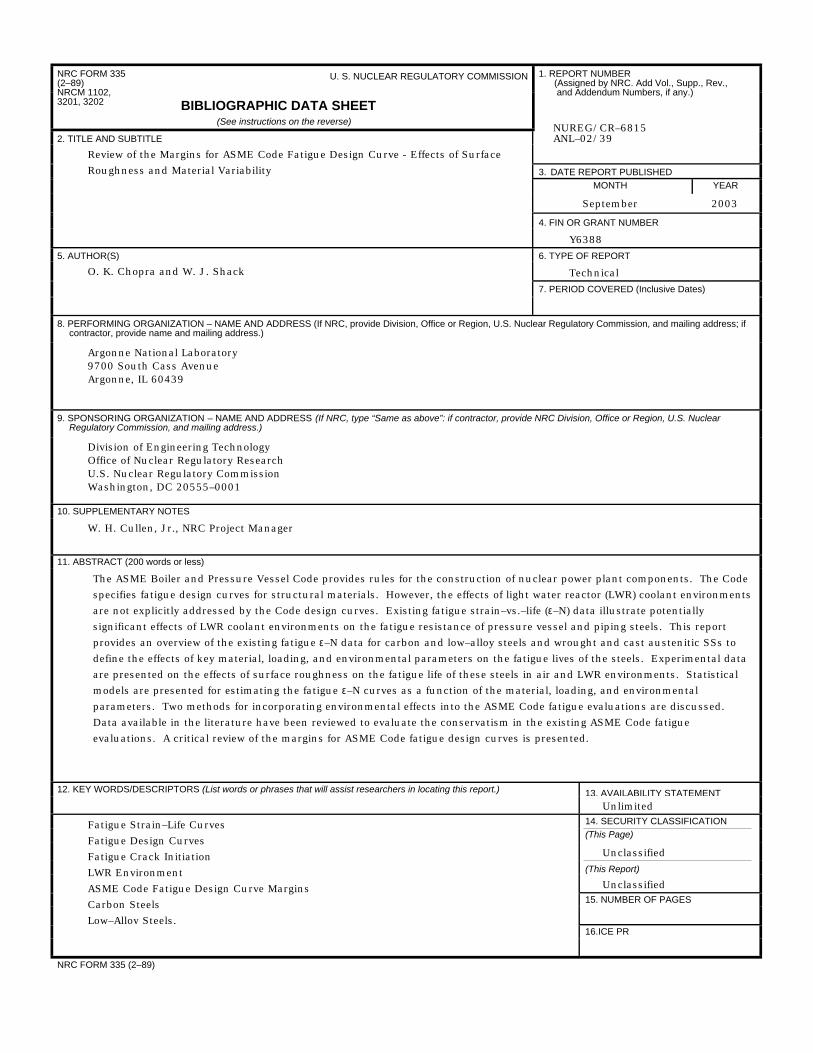
NRC FORM 335(2–89)NRCM 1102,3201, 3202

U. S. NUCLEAR REGULATORY COMMISSION

BIBLIOGRAPHIC DATA SHEET(See instructions on the reverse)

2. TITLE AND SUBTITLE

1. REPORT NUMBER (Assigned by NRC. Add Vol., Supp., Rev., and Addendum Numbers, if any.)

NUREG/CR–6815ANL–02/39

3. DATE REPORT PUBLISHED

MONTH YEAR

September 2003

4. FIN OR GRANT NUMBER

Review of the Margins for ASME Code Fatigue Design Curve - Effects of Surface

Roughness and Material Variability

Y6388

5. AUTHOR(S) 6. TYPE OF REPORT

Technical

7. PERIOD COVERED (Inclusive Dates)

O. K. Chopra and W. J. Shack

8. PERFORMING ORGANIZATION – NAME AND ADDRESS (If NRC, provide Division, Office or Region, U.S. Nuclear Regulatory Commission, and mailing address; ifcontractor, provide name and mailing address.)

Argonne National Laboratory9700 South Cass AvenueArgonne, IL 60439

9. SPONSORING ORGANIZATION – NAME AND ADDRESS (If NRC, type “Same as above”: if contractor, provide NRC Division, Office or Region, U.S. NuclearRegulatory Commission, and mailing address.)

Division of Engineering TechnologyOffice of Nuclear Regulatory ResearchU.S. Nuclear Regulatory CommissionWashington, DC 20555–0001

10. SUPPLEMENTARY NOTES

W. H. Cullen, Jr., NRC Project Manager

11. ABSTRACT (200 words or less)

The ASME Boiler and Pressure Vessel Code provides rules for the construction of nuclear power plant components. The Code

specifies fatigue design curves for structural materials. However, the effects of light water reactor (LWR) coolant environments

are not explicitly addressed by the Code design curves. Existing fatigue strain–vs.–life (e–N) data illustrate potentially

significant effects of LWR coolant environments on the fatigue resistance of pressure vessel and piping steels. This report

provides an overview of the existing fatigue e–N data for carbon and low–alloy steels and wrought and cast austenitic SSs to

define the effects of key material, loading, and environmental parameters on the fatigue lives of the steels. Experimental data

are presented on the effects of surface roughness on the fatigue life of these steels in air and LWR environments. Statistical

models are presented for estimating the fatigue e–N curves as a function of the material, loading, and environmental

parameters. Two methods for incorporating environmental effects into the ASME Code fatigue evaluations are discussed.

Data available in the literature have been reviewed to evaluate the conservatism in the existing ASME Code fatigue

evaluations. A critical review of the margins for ASME Code fatigue design curves is presented.

12. KEY WORDS/DESCRIPTORS (List words or phrases that will assist researchers in locating this report.) 13. AVAILABILITY STATEMENT

Unlimited14. SECURITY CLASSIFICATION

(This Page)

Unclassified

(This Report)

Unclassified15. NUMBER OF PAGES

Fatigue Strain–Life Curves

Fatigue Design Curves

Fatigue Crack Initiation

LWR Environment

ASME Code Fatigue Design Curve Margins

Carbon Steels

Low–Alloy Steels,16.ICE PR

NRC FORM 335 (2–89)

Review of the Margins for ASME Code Fatigue Design Curve ...

Documents

Transcript of Review of the Margins for ASME Code Fatigue Design Curve ...