Review of Probability Concepts ECON 6002 Econometrics Memorial University of Newfoundland Adapted...
62
ECON 6002 Econometrics Memorial University of Newfoundland Adapted from Vera Tabakova’s notes
Transcript of Review of Probability Concepts ECON 6002 Econometrics Memorial University of Newfoundland Adapted...

ECON 6002 Econometrics Memorial University of Newfoundland
Adapted from Vera Tabakova’s notes
B.1 Random Variables
B.2 Probability Distributions
B.3 Joint, Marginal and Conditional Probability
Distributions
B.4 Properties of Probability Distributions
B.5 Some Important Probability Distributions
A random variable is a variable whose value is unknown until it is observed.
A discrete random variable can take only a limited, or countable, number of values.
A continuous random variable can take any value on an interval.
The probability of an event is its “limiting relative frequency,” or the
proportion of time it occurs in the long-run.
The probability density function (pdf) for a discrete random
variable indicates the probability of each possible value occurring.
1 2
( )
( ) ( ) ( ) 1n
f x P X x
f x f x f x
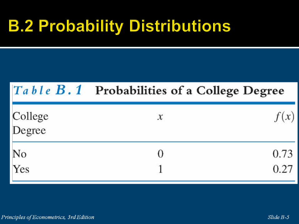
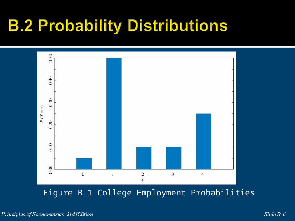
Figure B.1 College Employment Probabilities

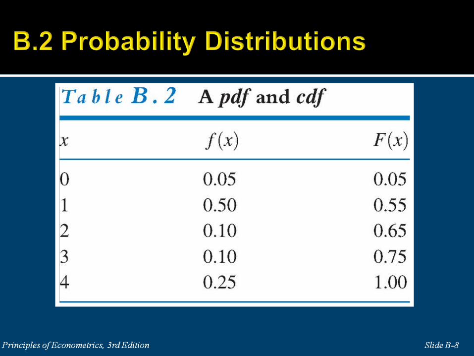
The cumulative distribution function (cdf) is an alternative way to
represent probabilities. The cdf of the random variable X, denoted
F(x), gives the probability that X is less than or equal to a specific
value x
F x P X x

For example, a binomial random variable X is the number of
successes in n independent trials of identical experiments with
probability of success p.
(1 )x n xnP X x f x p p
x
! where ! ( 1 2 2 1
! !
n nn n n n
x x n x

For example, if we know that the MUN basketball team has a chance
of winning of 70% (p=0.7) and we want to know how likely they are
to win at least 2 games in the next 3 weeks

For example, if we know that the MUN basketball team has a chance
of winning of 70% (p=0.7) and we want to know how likely they are
to win at least 2 games in the next 3 weeks
First: for winning only once in three weeks, likelihood is 0.189, see?
Times
n!x!n x! 3!
1!3 1! 3
px1 pn x 0.711 0.72 0.063
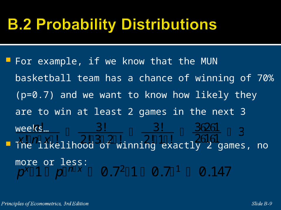
For example, if we know that the MUN basketball team has a chance
of winning of 70% (p=0.7) and we want to know how likely they are
to win at least 2 games in the next 3 weeks…
The likelihood of winning exactly 2 games, no more or less:
n!x!n x!
3!2!3 2!
3!2!1!
321211 3
px1 pn x 0.721 0.71 0.147

For example, if we know that the MUN basketball team has a chance
of winning of 70% (p=0.7) and we want to know how likely they are
to win at least 2 games in the next 3 weeks
So 3 times 0.147 = 0.441 is the likelihood of winning exactly 2 games

For example, if we know that the MUN basketball team has a chance
of winning of 70% (p=0.7) and we want to know how likely they are
to win at least 2 games in the next 3 weeks
And 0.343 is the likelihood of winning exactly 3 games
n!x!n x! 3!
3!3 3! 3!3!1 3!
3!1 1
px1 pn x 0.731 0.70 0.343
For example, if we know that the MUN basketball team has a chance of
winning of 70% (p=0.7) and we want to know how likely they are to win at
least 2 games in the next 3 weeks
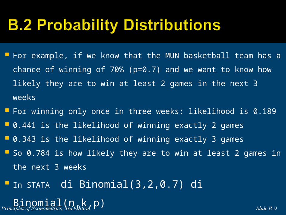
For winning only once in three weeks: likelihood is 0.189
0.441 is the likelihood of winning exactly 2 games
0.343 is the likelihood of winning exactly 3 games
So 0.784 is how likely they are to win at least 2 games in the next 3 weeks
In STATA di Binomial(3,2,0.7) di Binomial(n,k,p)

For example, if we know that the MUN basketball team has a chance
of winning of 70% (p=0.7) and we want to know how likely they are
to win at least 2 games in the next 3 weeks
So 0.784 is how likely they are to win at least 2 games in the next 3
weeks
In STATA di binomial(3,2,0.7) di
Binomial(n,k,p) is the likelihood of winning 1 or less
So we were looking for 1- binomial(3,2,0.7)
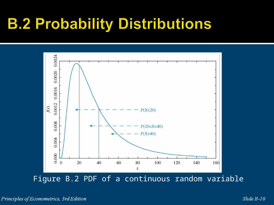
Figure B.2 PDF of a continuous random variable
40
20
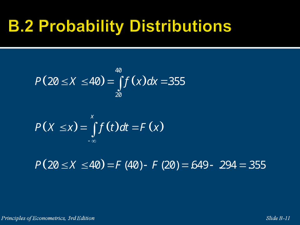
20 40 .355
20 40 (40) (20) .649 .294 .355
x
P X f x dx
P X x f t dt F x
P X F F

1 high school diploma or less
2 some college
3 four year college degree
4 advanced degree
X
0 if had no money earnings in 2002
1 if had positive money earnings in 2002Y
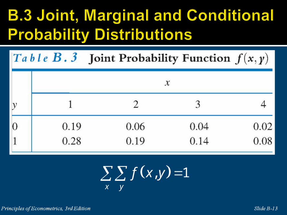
, 1x y
f x y

( ) ( , ) for each value can take
( ) ( , ) for each value can take
Xy
Yx
f x f x y X
f y f x y Y
4
1
, 0,1
1 .19 .06 .04 .02 .31
Yx
Y
f y f x y y
f

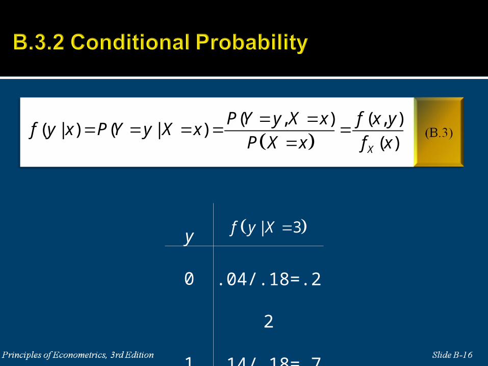
( , ) ( , )
( | ) ( | )( )X
P Y y X x f x yf y x P Y y X x
P X x f x
y
0 .04/.18=.22
1 .14/.18=.78
| 3f y X
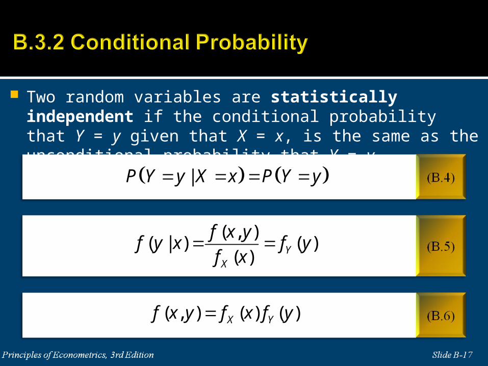
Two random variables are statistically independent if the conditional probability that Y = y given that X = x, is the same as the unconditional probability that Y = y.
|P Y y X x P Y y
( , )( | ) ( )
( ) YX
f x yf y x f y
f x
( , ) ( ) ( )X Yf x y f x f y

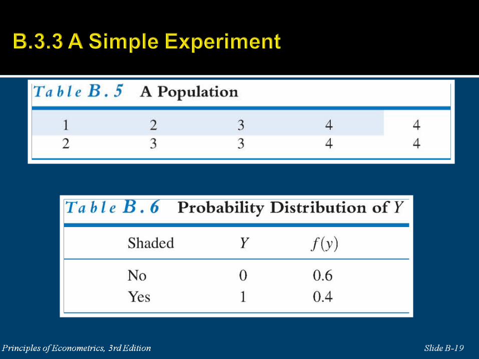
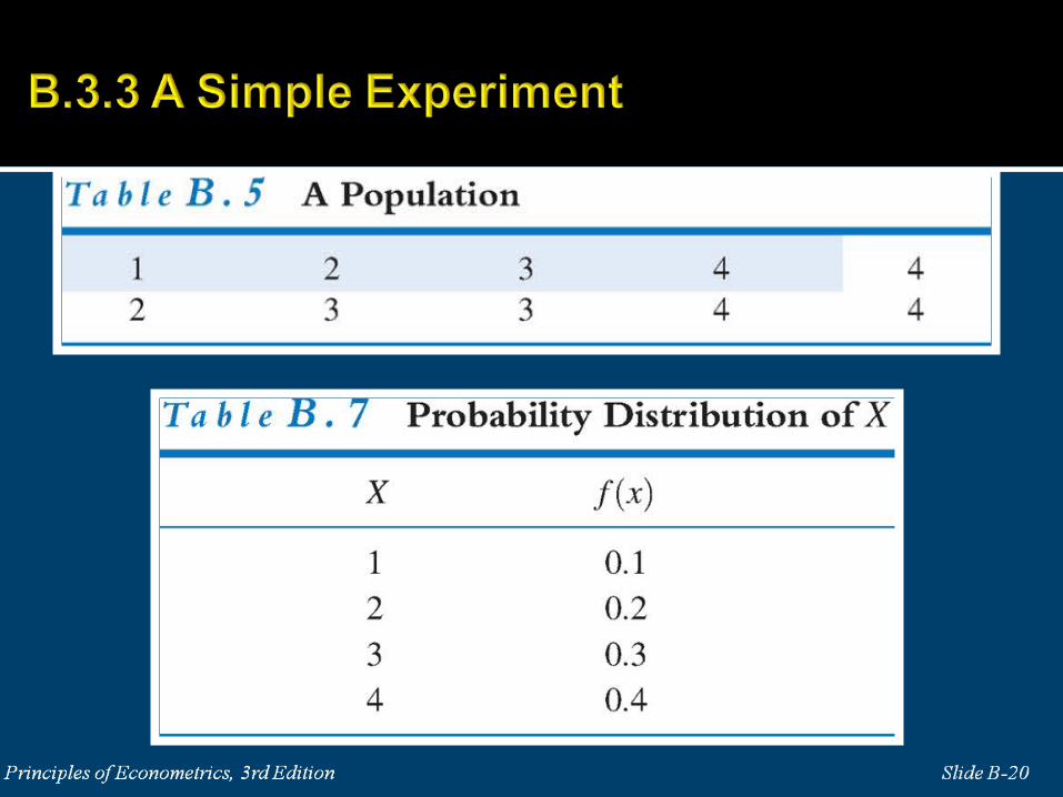
Y = 1 if shaded Y = 0 if clear
X = numerical value (1, 2, 3, or 4)


B.4.1 Mean, median and mode
For a discrete random variable the expected value is:
1 1 2 2[ ] n nE X x P X x x P X x x P X x
1 1 2 2
1
[ ] ( ) ( ) ( )
( ) ( )
n n
n
i ii x
E X x f x x f x x f x
x f x xf x
Where f is the discrete PDF of x

For a continuous random variable the expected value is:
The mean has a flaw as a measure of the center of a probability distribution in that it can be pulled by extreme values.
E X xf x dx
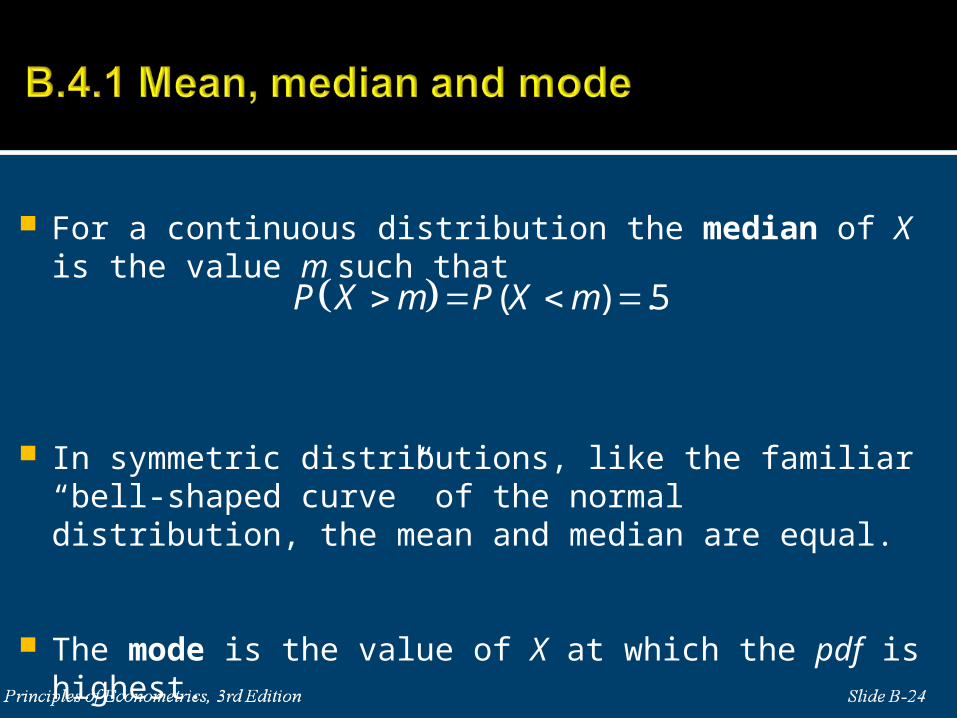
For a continuous distribution the median of X is the value m such that
In symmetric distributions, like the familiar “bell-shaped curve” of the normal distribution, the mean and median are equal.
The mode is the value of X at which the pdf is highest.
( ) .5P X m P X m
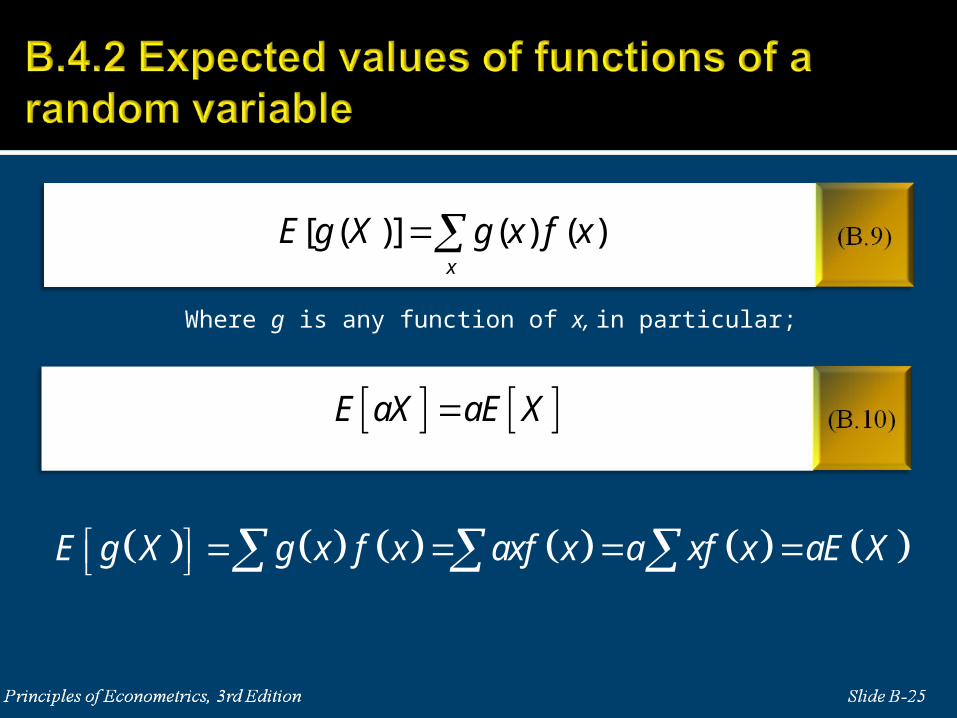
[ ( )] ( ) ( )x
E g X g x f x
E aX aE X
E g X g x f x axf x a xf x aE X
Where g is any function of x, in particular;

E aX b aE X b
1 2 1 2E g X g X E g X E g X

The variance of a discrete or continuous random variable X is the expected value of
2g X X E X
The variance
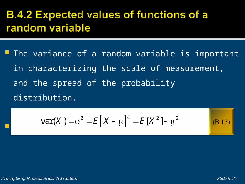
The variance of a random variable is important in characterizing the
scale of measurement, and the spread of the probability distribution.
Algebraically, letting E(X) = μ,
22 2 2var( ) [ ]X E X E X
The variance of a constant is?

Figure B.3 Distributions with different variances
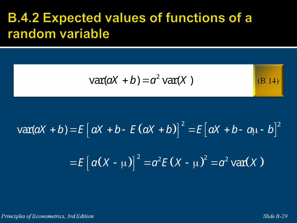
2var( ) var( )aX b a X
2 2
2 22 2
var( )
var
aX b E aX b E aX b E aX b a b
E a X a E X a X
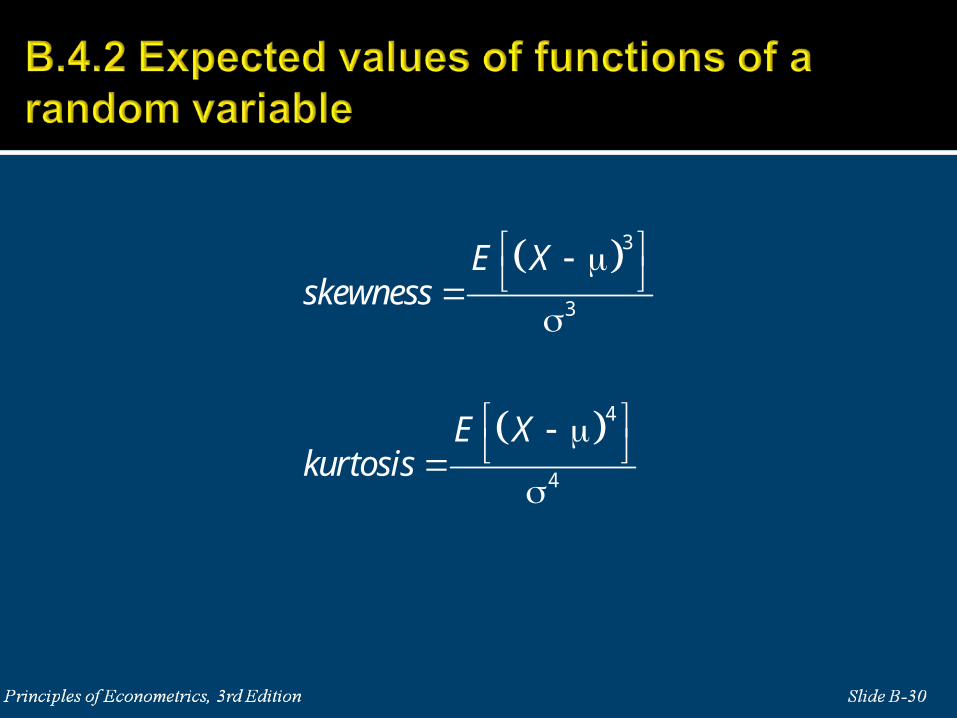
3
3
4
4
E Xskewness
E Xkurtosis
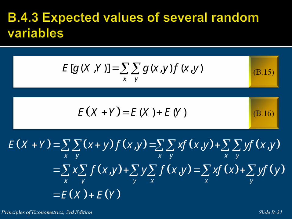
[ ( , )] ( , ) ( , )x y
E g X Y g x y f x y
( ) ( )E X Y E X E Y
, , ,
, ,
x y x y x y
x y y x x y
E X Y x y f x y xf x y yf x y
x f x y y f x y xf x yf y
E X E Y
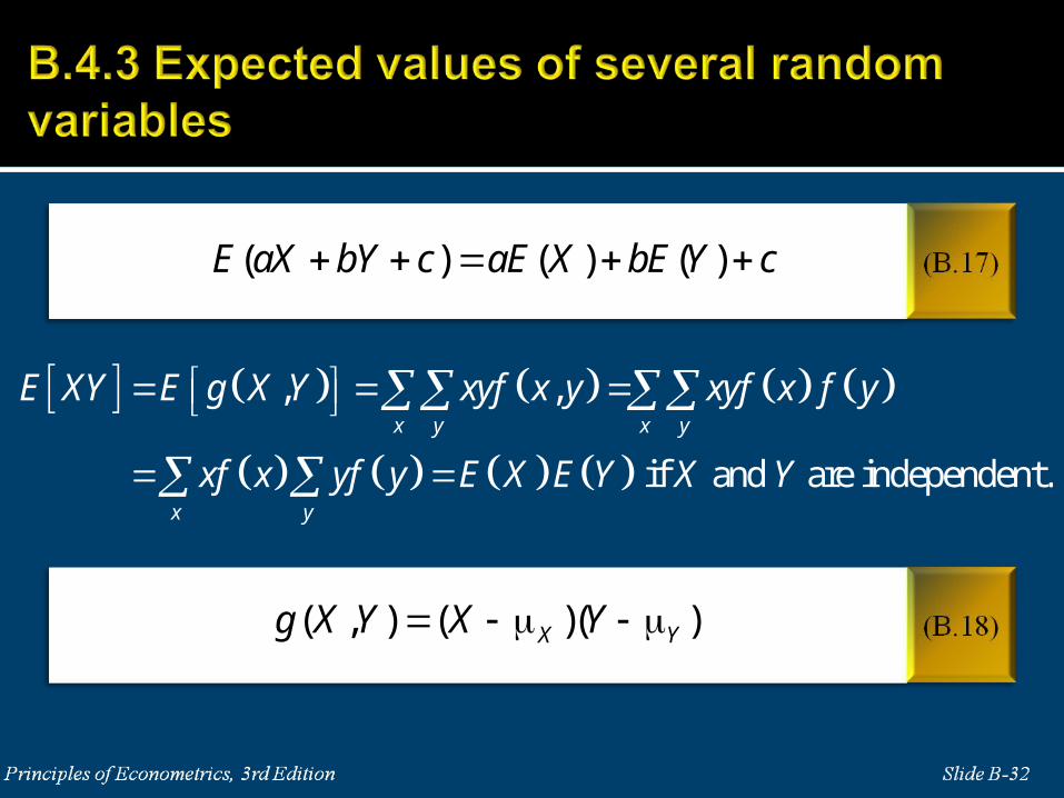
( ) ( ) ( )E aX bY c aE X bE Y c
, ,
if and are independent.
x y x y
x y
E XY E g X Y xyf x y xyf x f y
xf x yf y E X E Y X Y
( , ) ( )( )X Yg X Y X Y
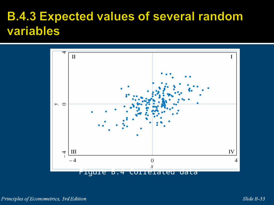
Figure B.4 Correlated data
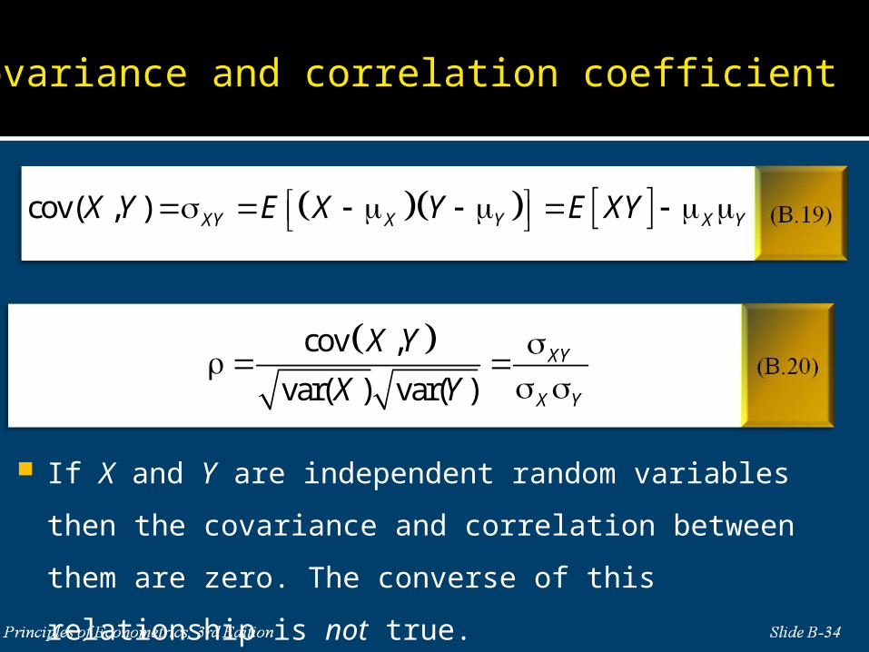
If X and Y are independent random variables then the covariance and
correlation between them are zero. The converse of this relationship
is not true.
cov( , ) XY X Y X YX Y E X Y E XY
cov ,
var( ) var( )XY
X Y
X Y
X Y
Covariance and correlation coefficient
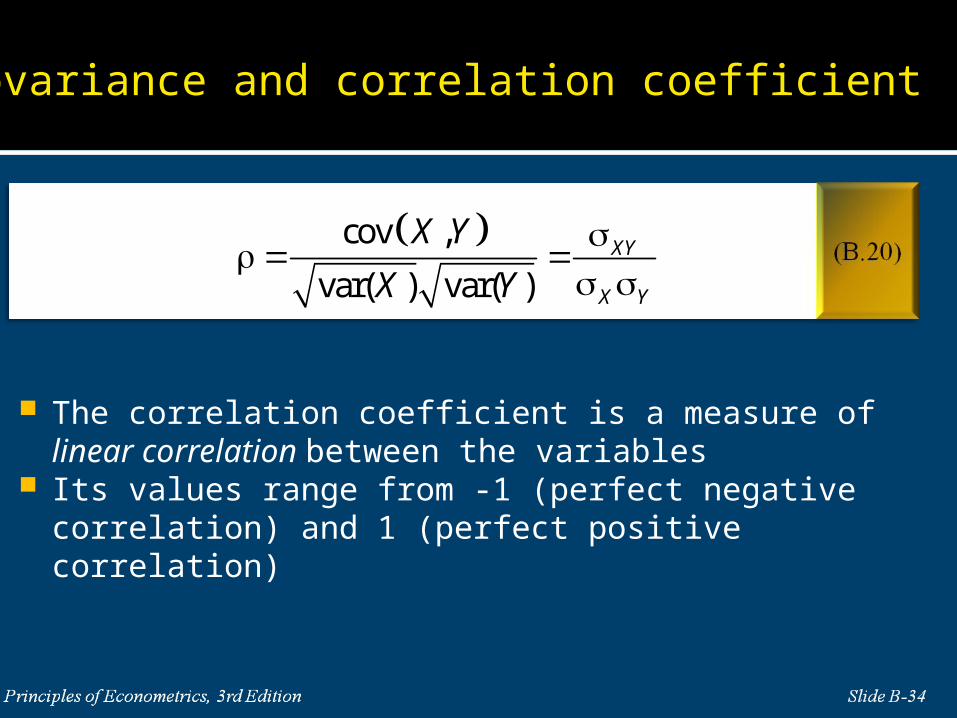
The correlation coefficient is a measure of linear correlation between the variables
Its values range from -1 (perfect negative correlation) and 1 (perfect positive correlation)
cov ,
var( ) var( )XY
X Y
X Y
X Y
Covariance and correlation coefficient

If a and b are constants then:
2 2var var( ) var( ) 2 cov( , )aX bY a X b Y ab X Y
var var( ) var( ) 2cov( , )X Y X Y X Y
var var( ) var( ) 2cov( , )X Y X Y X Y
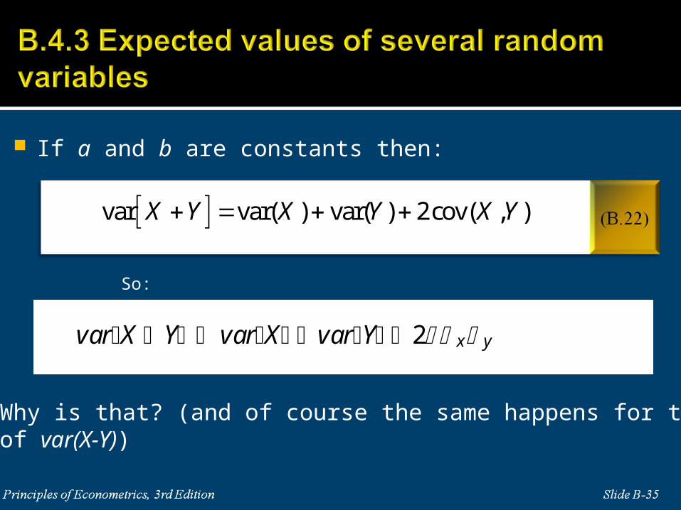
If a and b are constants then:
varX Y varX varY 2 x y
So:
Why is that? (and of course the same happens for the caseof var(X-Y))
var var( ) var( ) 2cov( , )X Y X Y X Y
If X and Y are independent then:
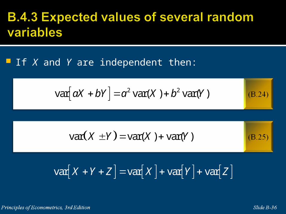
2 2var var( ) var( )aX bY a X b Y
var var( ) var( )X Y X Y
var var var varX Y Z X Y Z
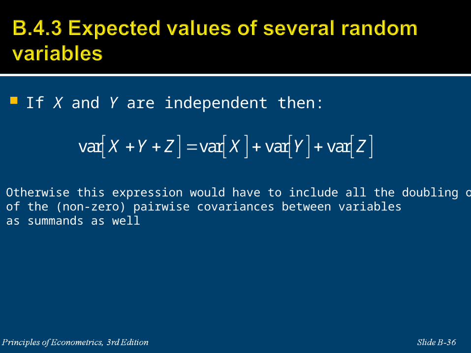
If X and Y are independent then:
var var var varX Y Z X Y Z
Otherwise this expression would have to include all the doubling of each of the (non-zero) pairwise covariances between variables as summands as well
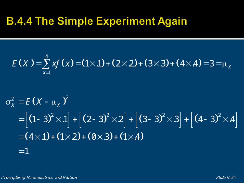
4
1
1 .1 2 .2 3 .3 4 .4 3 Xx
E X xf x
22
2 2 2 21 3 .1 2 3 .2 3 3 .3 4 3 .4
4 .1 1 .2 0 .3 1 .4
1
X XE X
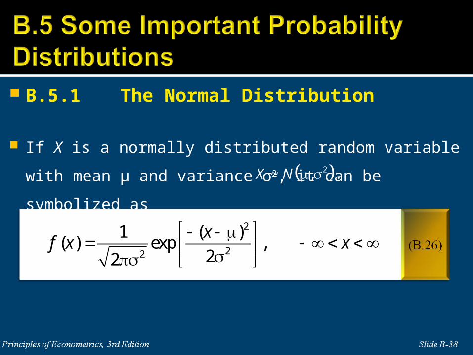
B.5.1 The Normal Distribution
If X is a normally distributed random variable with mean μ and
variance σ2, it can be symbolized as 2~ , .X N
2
22
1 ( )( ) exp ,
22
xf x x
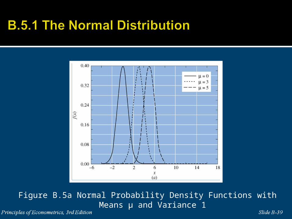
Figure B.5a Normal Probability Density Functions with Means μ and Variance 1
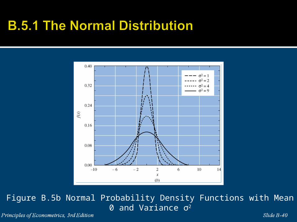
Figure B.5b Normal Probability Density Functions with Mean 0 and Variance σ2

A standard normal random variable is one that has a normal
probability density function with mean 0 and variance 1.
The cdf for the standardized normal variable Z is
~ (0,1)X
Z N
( ) .z P Z z

[ ]X a a a
P X a P P Z
[ ] 1X a a a
P X a P P Z
[ ]a b b a
P a X b P Z

A weighted sum of normal random variables has a normal
distribution.
21 1 1
22 2 2
~ ,
~ ,
X N
X N
2 2 2 2 21 1 2 2 1 1 2 2 1 1 2 2 1 2 12~ , 2Y YY a X a X N a a a a a a

2 2 2 2
1 2 ( )~m mV Z Z Z
2( )
2( )
[ ]
var[ ] var 2
m
m
E V E m
V m
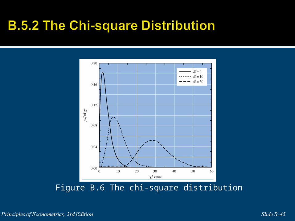
Figure B.6 The chi-square distribution

A “t” random variable (no upper case) is formed by dividing a
standard normal random variable by the square root of an
independent chi-square random variable, , that has been
divided by its degrees of freedom m.
( )~ m
Zt t
Vm
~ 0,1Z N
2( )~ mV

Figure B.7 The standard normal and t(3) probability density functions
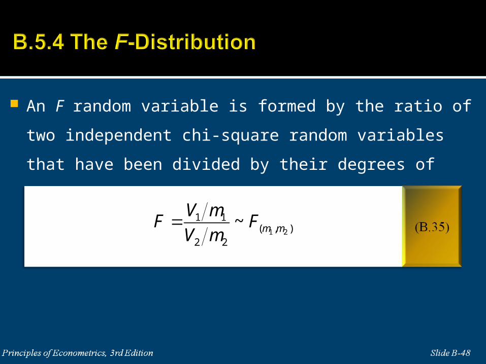
An F random variable is formed by the ratio of two independent chi-
square random variables that have been divided by their degrees of
freedom.
1 2
1 1( , )
2 2
~ m m
V mF F
V m

Figure B.8 The probability density function of an F random variable
Slide B-62Principles of Econometrics, 3rd Edition