Review of Matrix Algebra -...
108
Review of Matrix Algebra
Transcript of Review of Matrix Algebra -...

Review of Matrix Algebra
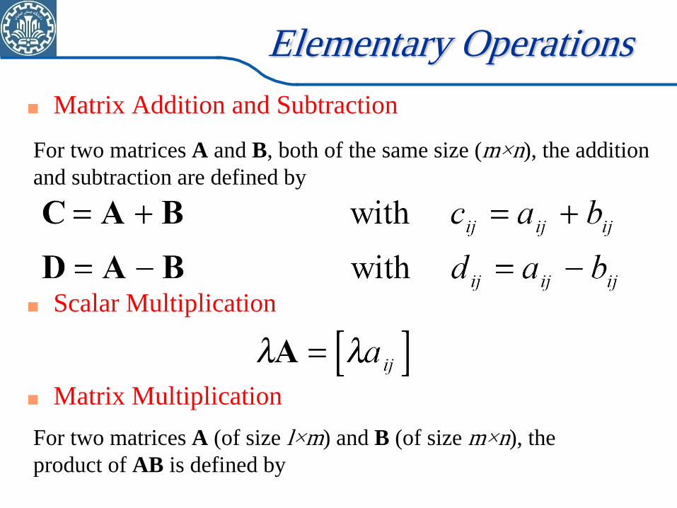
Matrix Addition and Subtraction
Elementary Operations
For two matrices A and B, both of the same size (m×n), the addition
and subtraction are defined by
Scalar Multiplication
Matrix Multiplication
For two matrices A (of size l×m) and B (of size m×n), the
product of AB is defined by
Elementary Operations
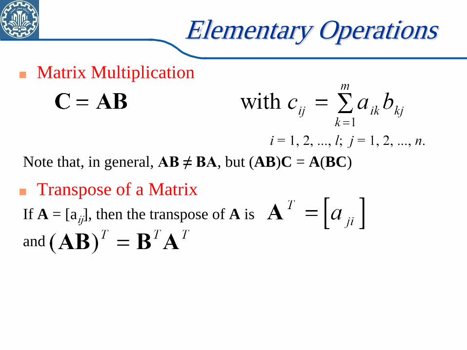
Matrix Multiplication
Note that, in general, AB ≠ BA, but (AB)C = A(BC)
Transpose of a Matrix
If A = [aij], then the transpose of A is
and
Elementary Operations
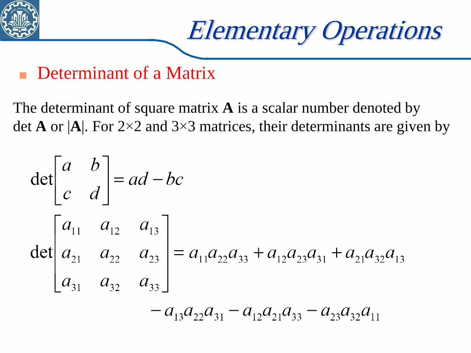
Determinant of a Matrix
The determinant of square matrix A is a scalar number denoted by
det A or |A|. For 2×2 and 3×3 matrices, their determinants are given by
Elementary Operations
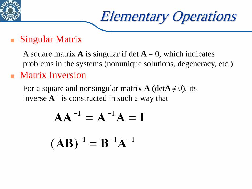
Singular Matrix
A square matrix A is singular if det A = 0, which indicates
problems in the systems (nonunique solutions, degeneracy, etc.)
Matrix Inversion
For a square and nonsingular matrix A (detA ≠ 0), its
inverse A-1 is constructed in such a way that
Elementary Operations
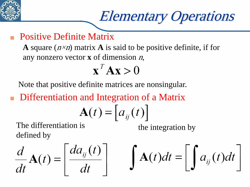
Positive Definite Matrix A square (n×n) matrix A is said to be positive definite, if for
any nonzero vector x of dimension n,
Differentiation and Integration of a Matrix
Note that positive definite matrices are nonsingular.
The differentiation is
defined by the integration by
Review of Matrix Algebra
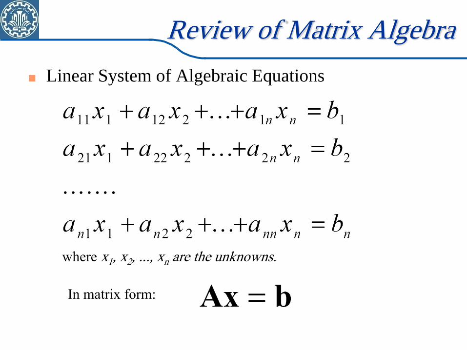
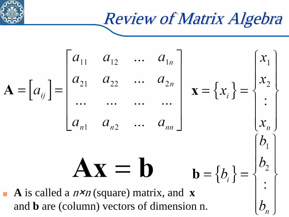
Linear System of Algebraic Equations
where x1, x2, ..., xn are the unknowns.
In matrix form:
Review of Matrix Algebra
A is called a n×n (square) matrix, and x
and b are (column) vectors of dimension n.
Review of Matrix Algebra
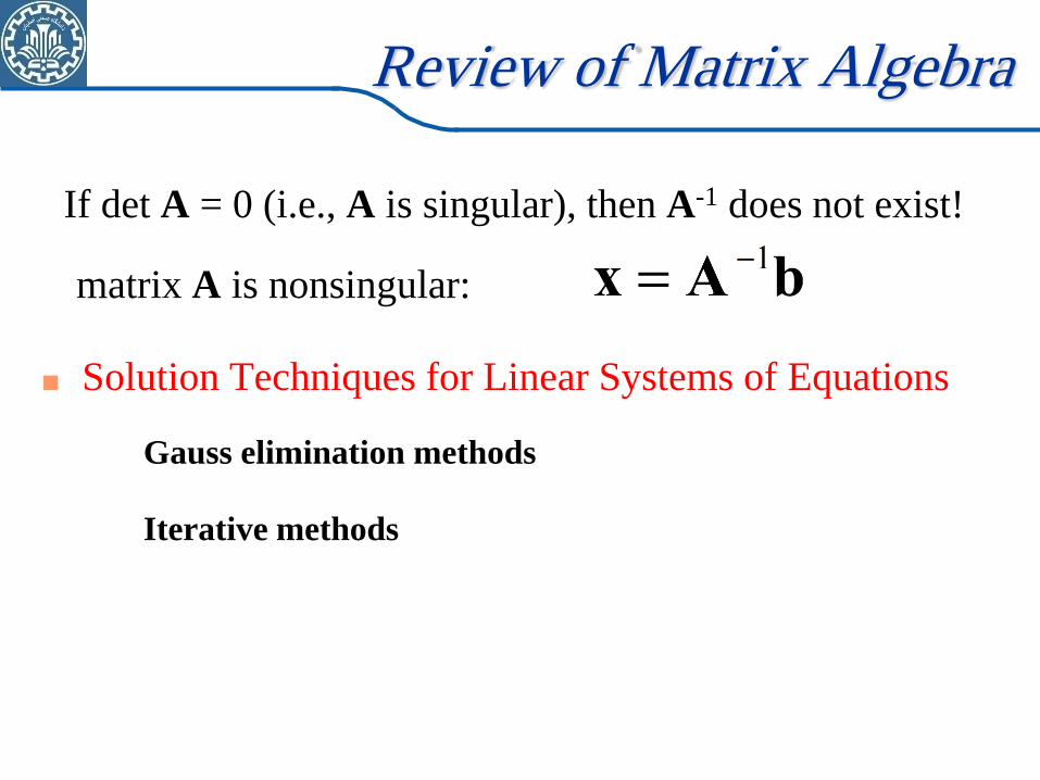
If det A = 0 (i.e., A is singular), then A-1 does not exist!
matrix A is nonsingular:
Solution Techniques for Linear Systems of Equations
Gauss elimination methods
Iterative methods

MATLAB Fundamentals
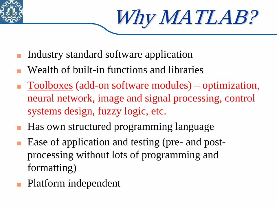
Why MATLAB?
Industry standard software application
Wealth of built-in functions and libraries
Toolboxes (add-on software modules) – optimization,
neural network, image and signal processing, control
systems design, fuzzy logic, etc.
Has own structured programming language
Ease of application and testing (pre- and post-
processing without lots of programming and
formatting)
Platform independent
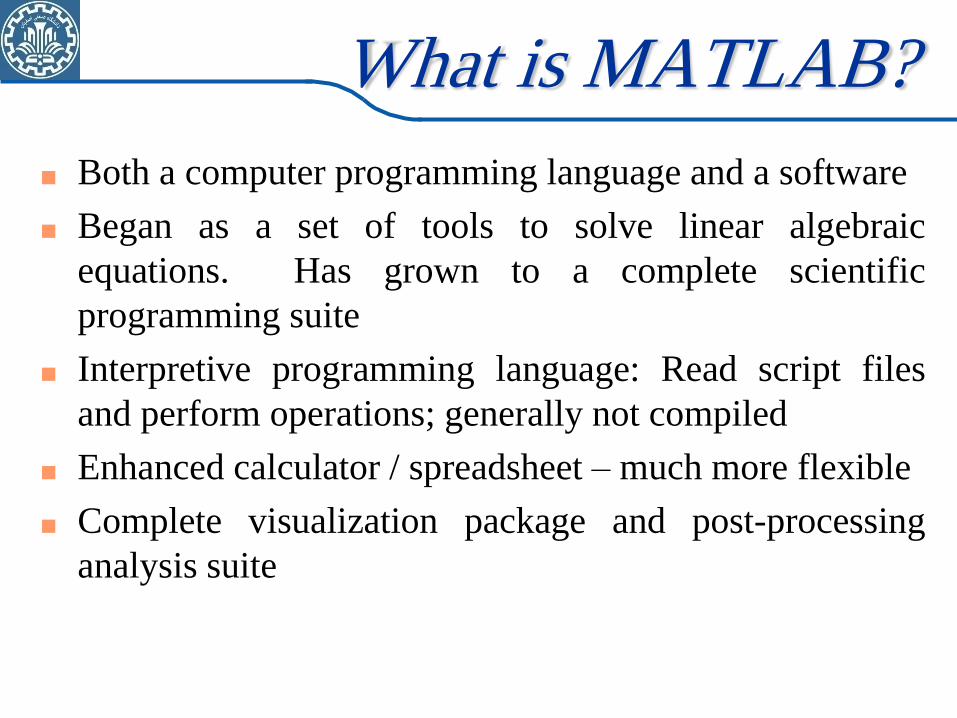
Both a computer programming language and a software
Began as a set of tools to solve linear algebraic
equations. Has grown to a complete scientific
programming suite
Interpretive programming language: Read script files
and perform operations; generally not compiled
Enhanced calculator / spreadsheet – much more flexible
Complete visualization package and post-processing
analysis suite
What is MATLAB?
MATLAB
MATLAB is a numerical analysis system
Can write “programs”, but they are not formally
compiled
Should still use structured programming
Should still use comments
Comments are indicated by “%” at the beginning of
the line
MATLAB Windows Command Window
-- enter commands and data
-- print results
Graphics Window
-- display plots and graphs
Edit Window
-- create and modify m-files
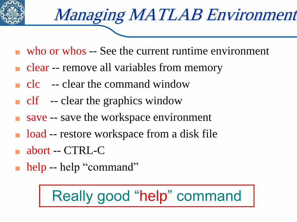
who or whos -- See the current runtime environment
clear -- remove all variables from memory
clc -- clear the command window
clf -- clear the graphics window
save -- save the workspace environment
load -- restore workspace from a disk file
abort -- CTRL-C
help -- help “command”
Really good “help” command
Managing MATLAB Environment
MATLAB Syntax
No complicated rules
Perhaps the most important thing to
remember is semicolons (;) at the end of a
line to suppress output
diary “filename” saves a text record of
session
diary off turns it off
MATLAB
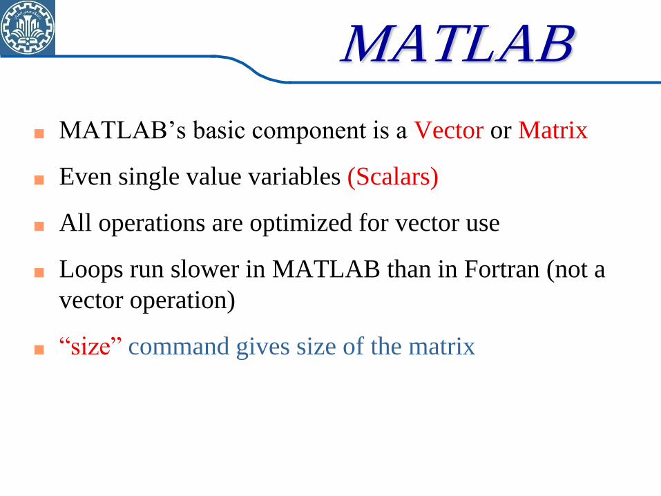
MATLAB‟s basic component is a Vector or Matrix
Even single value variables (Scalars)
All operations are optimized for vector use
Loops run slower in MATLAB than in Fortran (not a
vector operation)
“size” command gives size of the matrix
Scalars, Vectors, Matrices
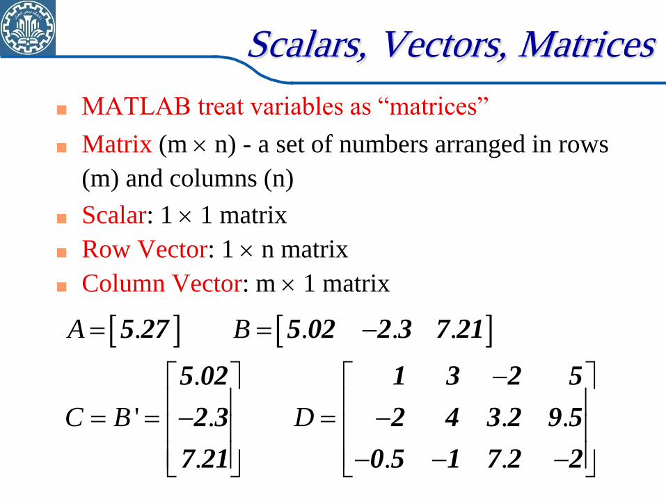
MATLAB treat variables as “matrices”
Matrix (m n) - a set of numbers arranged in rows
(m) and columns (n)
Scalar: 1 1 matrix
Row Vector: 1 n matrix
Column Vector: m 1 matrix
. . . .
.
' . . .
. . .
A B
C B D
5 27 5 02 2 3 7 21
5 02 1 3 2 5
2 3 2 4 3 2 9 5
7 21 0 5 1 7 2 2
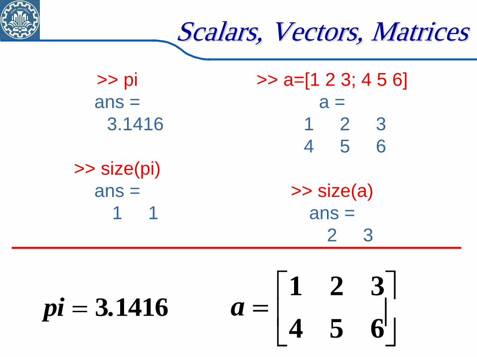
>> pi
ans =
3.1416
>> size(pi)
ans =
1 1
>> a=[1 2 3; 4 5 6]
a =
1 2 3
4 5 6
>> size(a)
ans =
2 3
a= 14163.pi
654
321a
Scalars, Vectors, Matrices
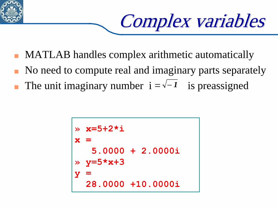
MATLAB handles complex arithmetic automatically
No need to compute real and imaginary parts separately
The unit imaginary number i = is preassigned 1
» x=5+2*i
x =
5.0000 + 2.0000i
» y=5*x+3
y =
28.0000 +10.0000i
Complex variables
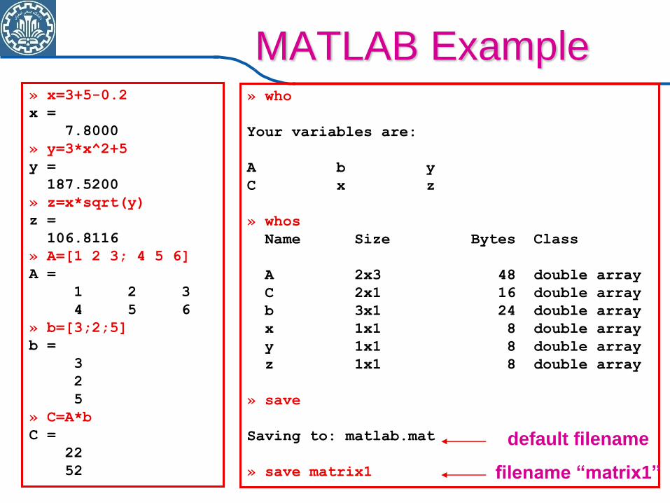
MATLAB Example » x=3+5-0.2
x =
7.8000
» y=3*x^2+5
y =
187.5200
» z=x*sqrt(y)
z =
106.8116
» A=[1 2 3; 4 5 6]
A =
1 2 3
4 5 6
» b=[3;2;5]
b =
3
2
5
» C=A*b
C =
22
52
» who
Your variables are:
A b y
C x z
» whos
Name Size Bytes Class
A 2x3 48 double array
C 2x1 16 double array
b 3x1 24 double array
x 1x1 8 double array
y 1x1 8 double array
z 1x1 8 double array
» save
Saving to: matlab.mat
» save matrix1
default filename
filename “matrix1”
Data types
All numbers are double precision
Text is stored as arrays of characters
You don‟t have to declare the type of data (defined
when running)
MATLAB is case-sensitive!!!
Variable Names Usually, the name is identified with the problem
Variable names may consist of up to 31 characters
Variable names may be alphabetic, digits, and the
underscore character ( _ )
Variable names must start with a letter
ABC, A1, C56, CVEN_302
day, year, iteration, max
time, velocity, distance, area, density,
pressure
Time, TIME, time (case sensitive!!)
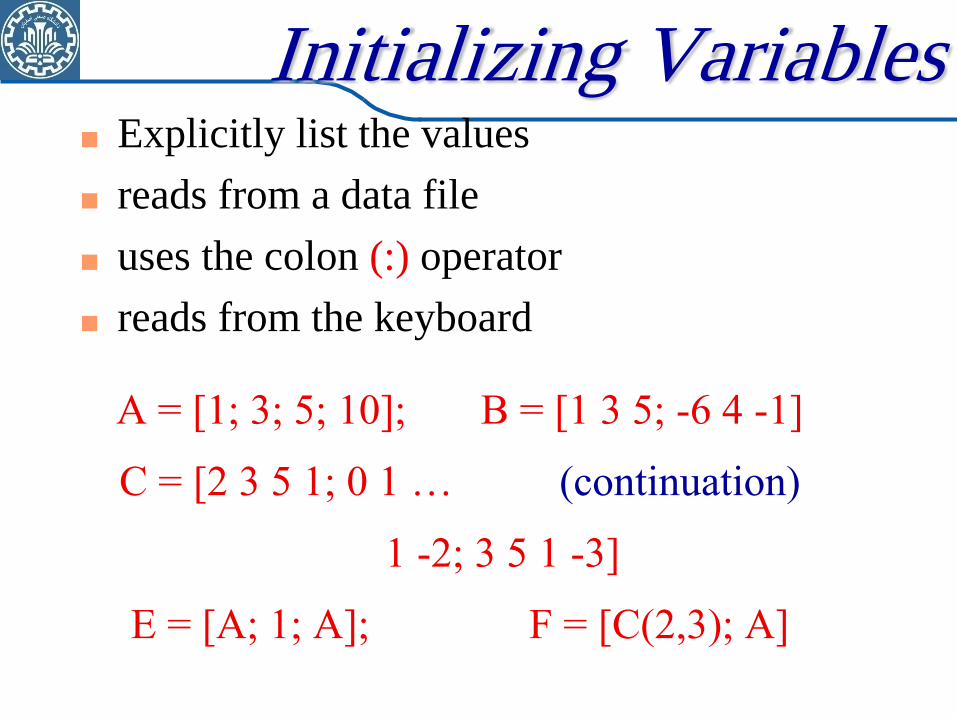
Initializing Variables Explicitly list the values
reads from a data file
uses the colon (:) operator
reads from the keyboard
A = [1; 3; 5; 10]; B = [1 3 5; -6 4 -1]
C = [2 3 5 1; 0 1 … (continuation)
1 -2; 3 5 1 -3]
E = [A; 1; A]; F = [C(2,3); A]
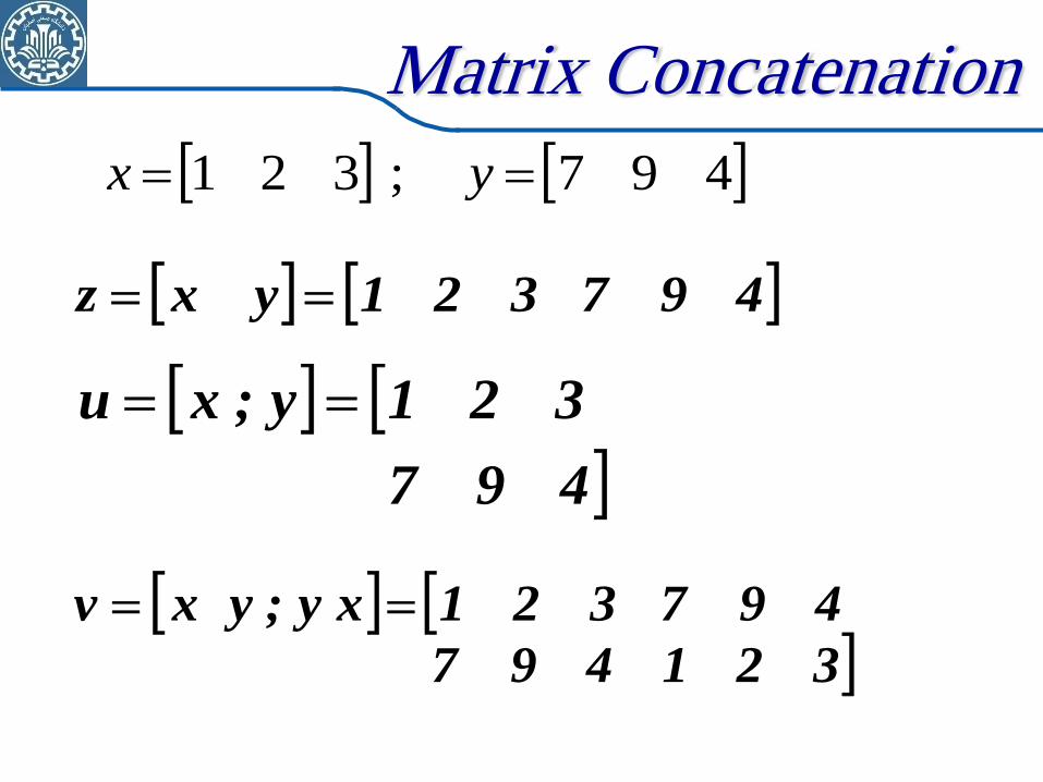
Matrix Concatenation
497 ; 321 yx
497321yxz
321497
497321 xy ;y xv
497
321y ;x u
Colon Operator
41
12
10
52
F
410
123
101
521
C
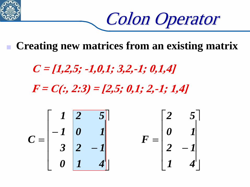
Creating new matrices from an existing matrix
C = [1,2,5; -1,0,1; 3,2,-1; 0,1,4]
F = C(:, 2:3) = [2,5; 0,1; 2,-1; 1,4]
Colon Operator
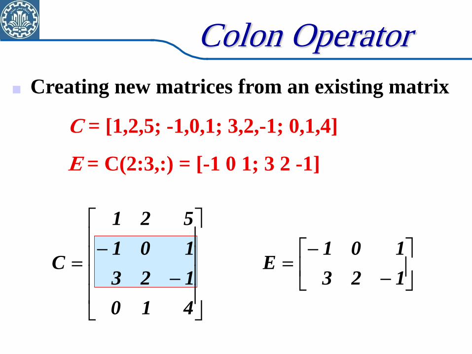
Creating new matrices from an existing matrix
123
101E
410
123
101
521
C
C = [1,2,5; -1,0,1; 3,2,-1; 0,1,4]
E = C(2:3,:) = [-1 0 1; 3 2 -1]
Colon Operator
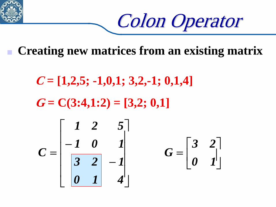
Creating new matrices from an existing matrix
C = [1,2,5; -1,0,1; 3,2,-1; 0,1,4]
G = C(3:4,1:2) = [3,2; 0,1]
10
23G
410
123
101
521
C
Colon Operator
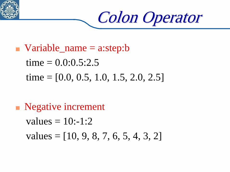
Variable_name = a:step:b
time = 0.0:0.5:2.5
time = [0.0, 0.5, 1.0, 1.5, 2.0, 2.5]
Negative increment
values = 10:-1:2
values = [10, 9, 8, 7, 6, 5, 4, 3, 2]
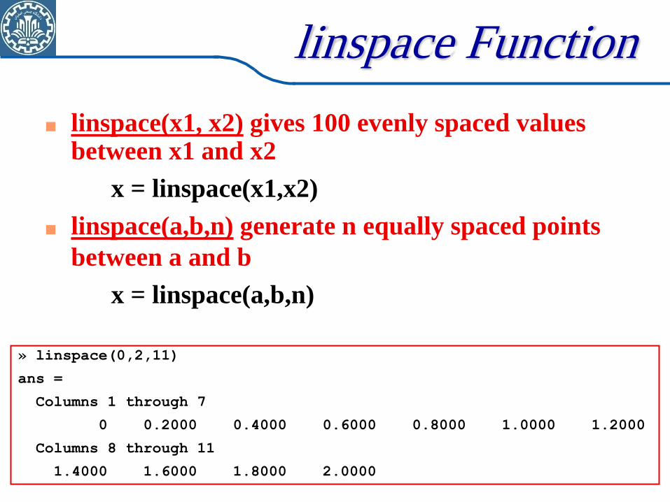
linspace Function
linspace(x1, x2) gives 100 evenly spaced values between x1 and x2
x = linspace(x1,x2)
linspace(a,b,n) generate n equally spaced points
between a and b
x = linspace(a,b,n)
» linspace(0,2,11)
ans =
Columns 1 through 7
0 0.2000 0.4000 0.6000 0.8000 1.0000 1.2000
Columns 8 through 11
1.4000 1.6000 1.8000 2.0000
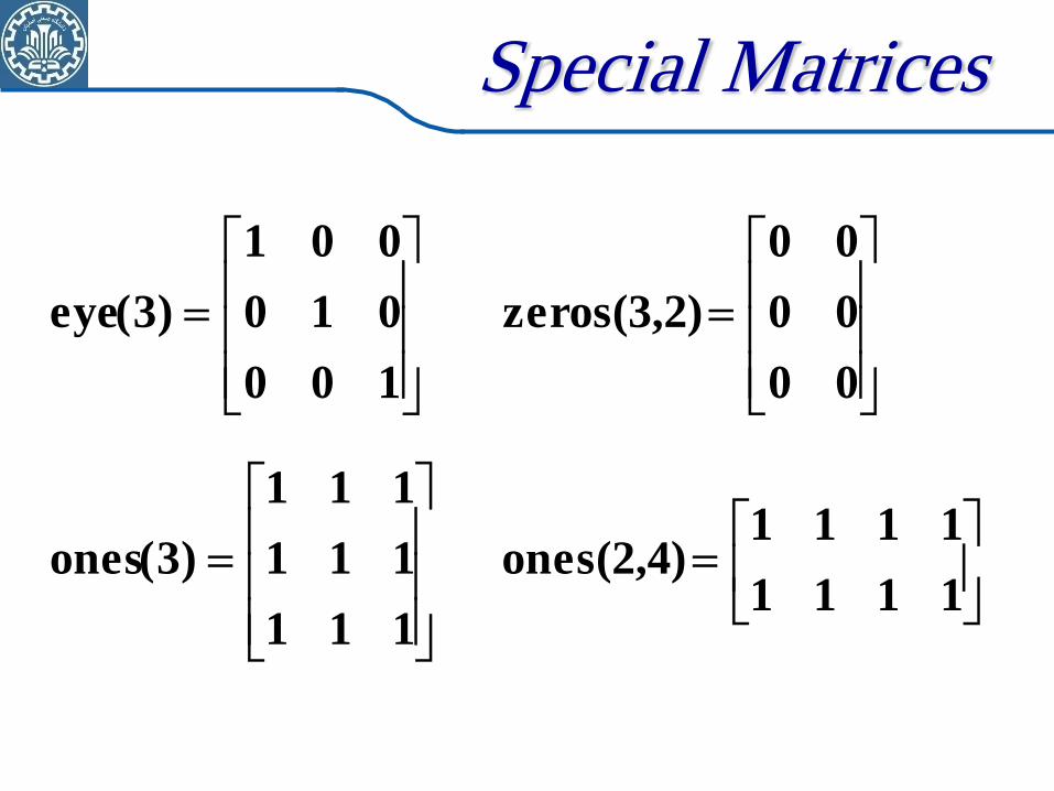
Special Matrices
1111
1111ones(2,4)
111
111
111
)3(ones
00
00
00
zeros(3,2)
100
010
001
)3(eye
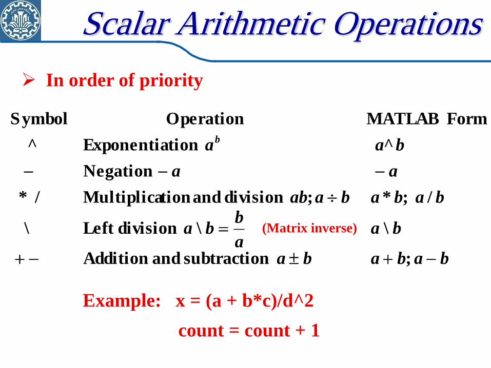
Scalar Arithmetic Operations
In order of priority
bababa
baa
bba
bababaab
aa
baab
; nsubtractio and Addition
\ \ division Left\
/ ;* ; division and tionMultiplica/ *
Negation
^ tionExponentia^
Form MATLABOperation Symbol
(Matrix inverse)
Example: x = (a + b*c)/d^2
count = count + 1
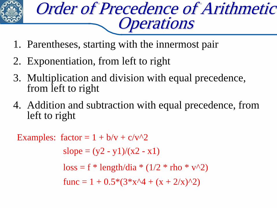
Order of Precedence of Arithmetic Operations
1. Parentheses, starting with the innermost pair
2. Exponentiation, from left to right
3. Multiplication and division with equal precedence, from left to right
4. Addition and subtraction with equal precedence, from left to right
Examples: factor = 1 + b/v + c/v^2
slope = (y2 - y1)/(x2 - x1)
loss = f * length/dia * (1/2 * rho * v^2)
func = 1 + 0.5*(3*x^4 + (x + 2/x)^2)
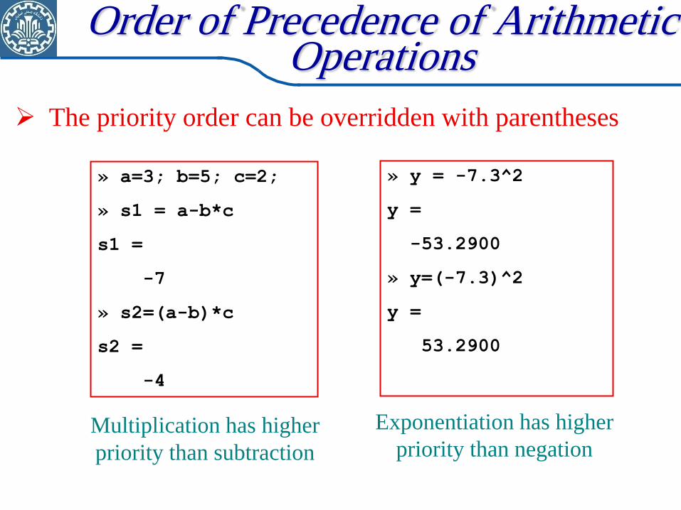
Order of Precedence of Arithmetic Operations
The priority order can be overridden with parentheses
» y = -7.3^2
y =
-53.2900
» y=(-7.3)^2
y =
53.2900
» a=3; b=5; c=2;
» s1 = a-b*c
s1 =
-7
» s2=(a-b)*c
s2 =
-4
Exponentiation has higher
priority than negation Multiplication has higher
priority than subtraction
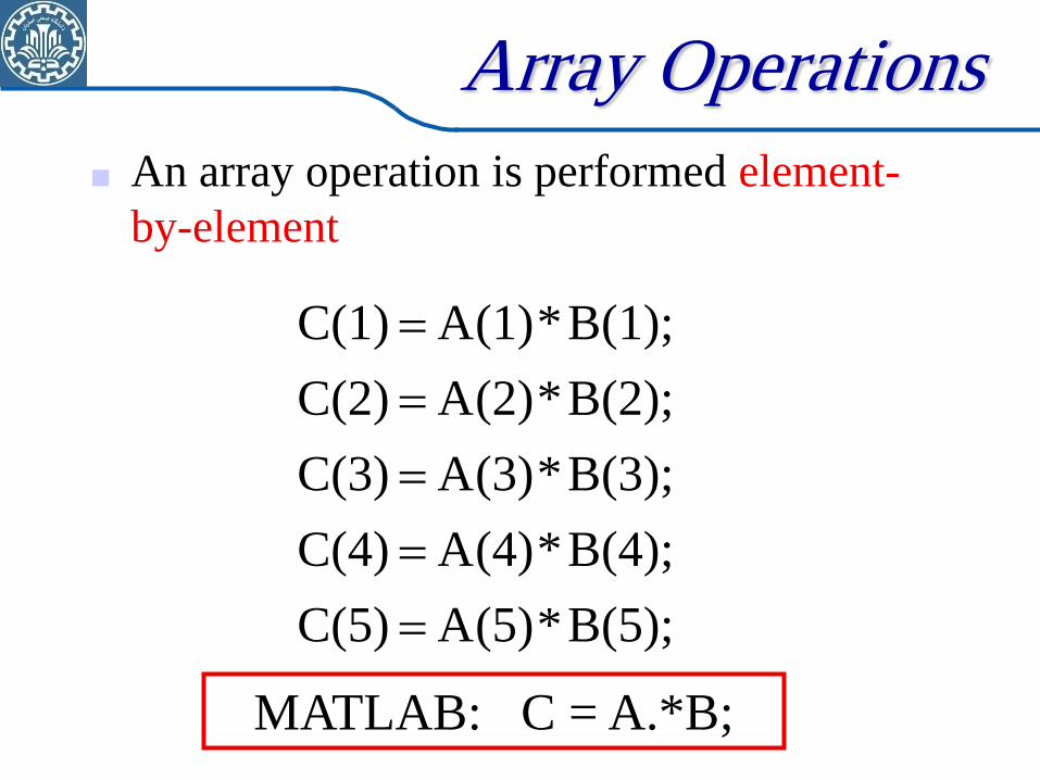
Array Operations
An array operation is performed element-
by-element
MATLAB: C = A.*B;
B(5);*A(5) C(5)
B(4);*A(4) C(4)
B(3);*A(3) C(3)
B(2);*A(2) C(2)
B(1);*A(1) C(1)
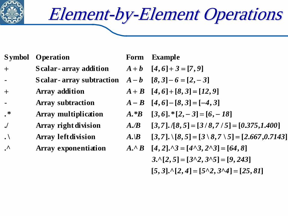
Element-by-Element Operations
] ,[]^ ,^[] ,[].^ ,[
] ,[]^ ,^[] ,[.^
] ,[]^ ,^[].^ ,[.^tionexponentia Array.^
].,.[]\ ,\[] ,[\]. ,[division left Array\.
].,.[]/ ,/[] ,/[]. ,[division right Array./
] ,[] ,[*]. ,[tionmultiplica Array*.
] ,[] ,[] ,[nsubtractio Array-
] ,[] ,[] ,[addition Array
] ,[] ,[nsubtractio array-Scalar-
] ,[] ,[addition array-Scalar
ExampleFormOperationSymbol
812543254235
24395323523
8643234324BA
71430667257835873A.\B
4001375057835873A./B
1863263A.*B
343864BA
9123864BA
32638bA
97364bA
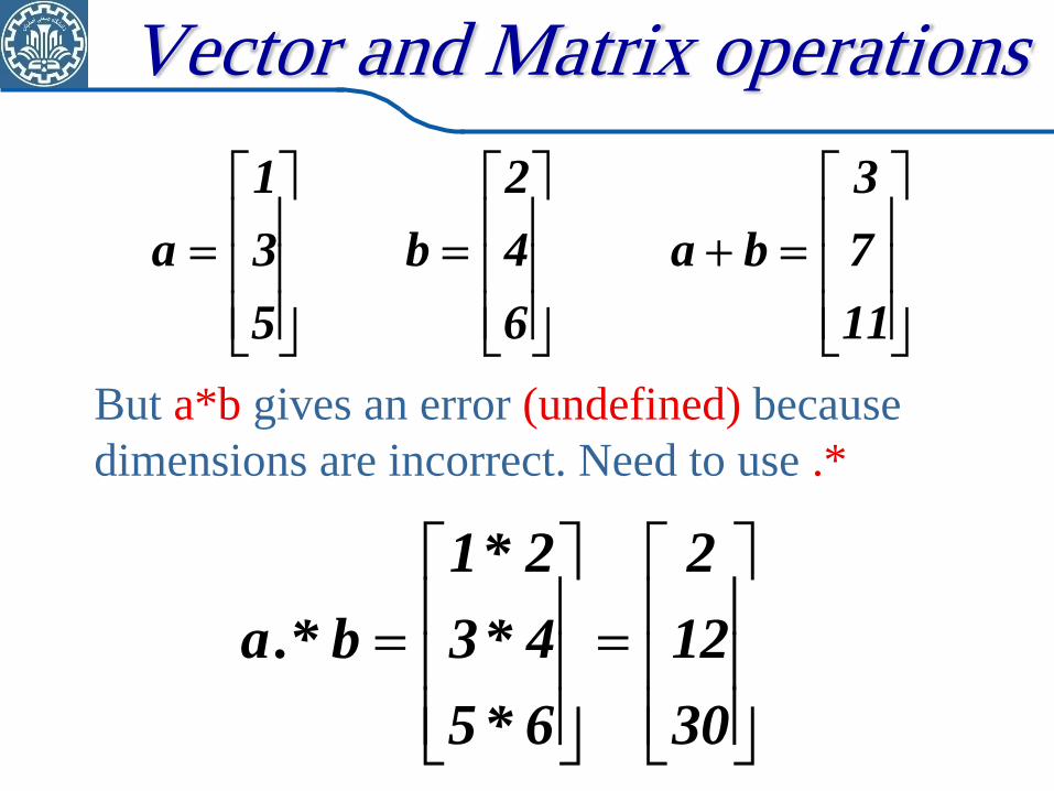
Vector and Matrix operations
But a*b gives an error (undefined) because
dimensions are incorrect. Need to use .*
11
7
3
ba
6
4
2
b
5
3
1
a
30
12
2
6*5
4*3
2*1
b.*a
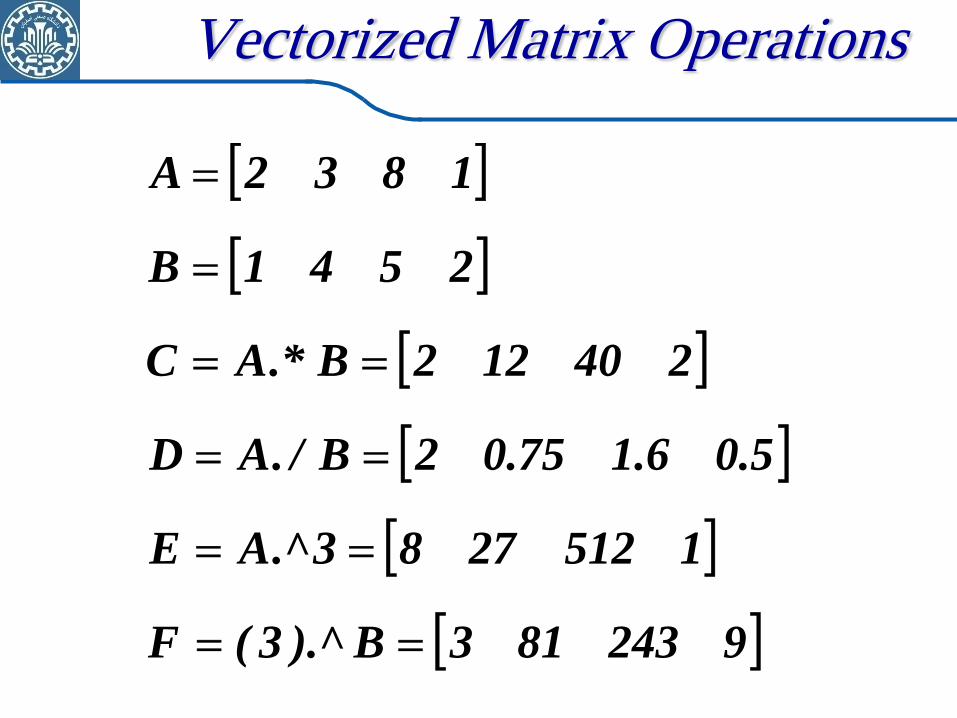
Vectorized Matrix Operations
9243813B).^3(F
15122783.^AE
5.06.175.02B/.AD
240122B.*AC
2541B
1832A
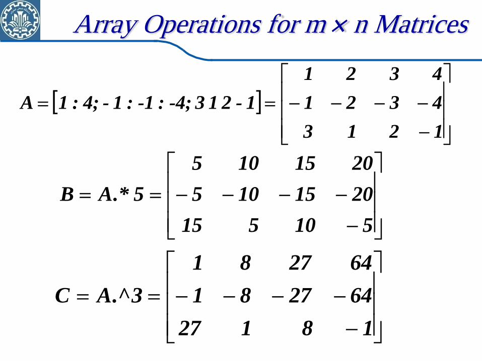
Array Operations for m n Matrices
510515
2015105
2015105
5.*AB
1213
4321
4321
1 - 21 3-4;:-1:1 -4;:1A
18127
642781
642781
3.^AC
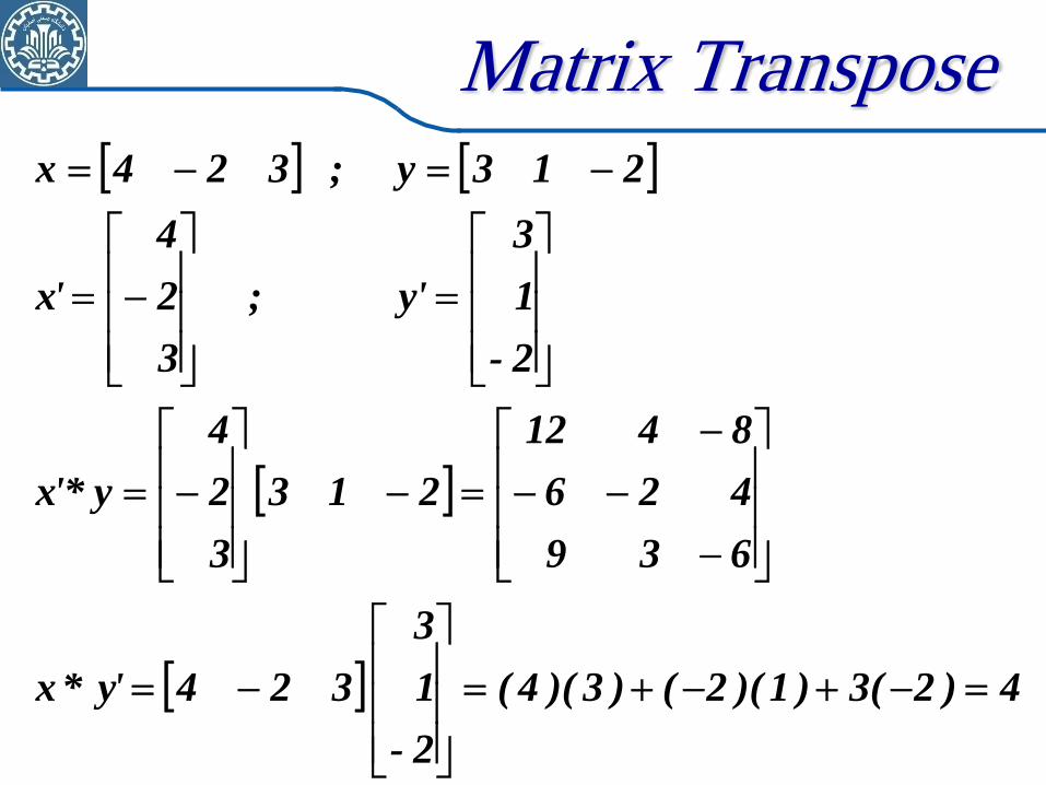
Matrix Transpose
4)2(3)1)(2()3)(4(
2-
1
3
324'y*x
639
426
8412
213
3
2
4
y'*x
2-
1
3
y' ;
3
2
4
'x
213y ; 324x
Built-in Functions
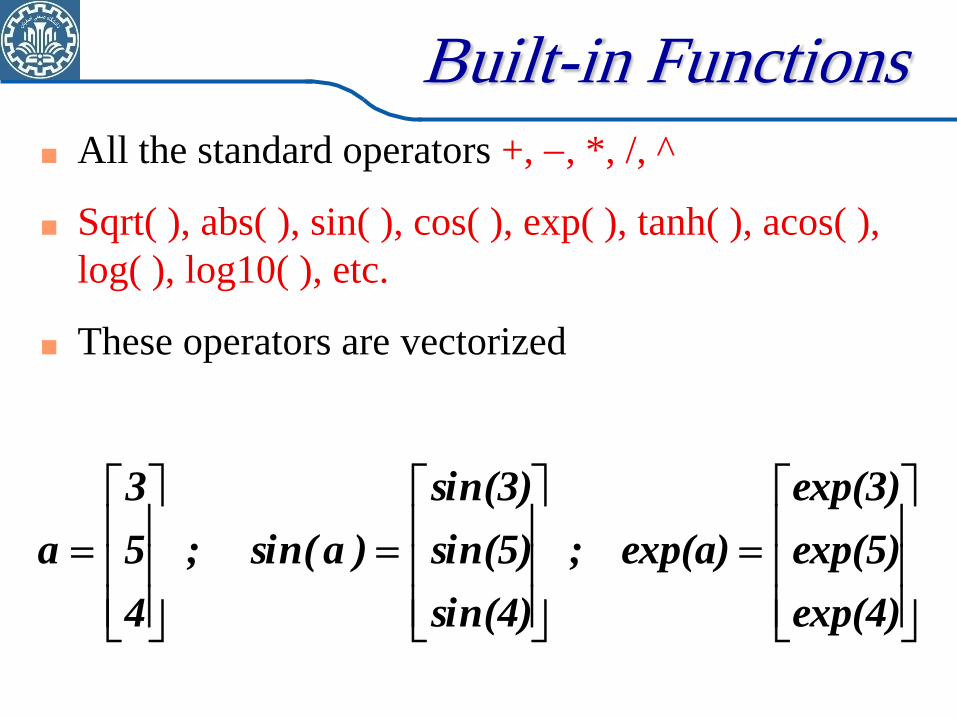
All the standard operators +, , *, /, ^
Sqrt( ), abs( ), sin( ), cos( ), exp( ), tanh( ), acos( ),
log( ), log10( ), etc.
These operators are vectorized
exp(4)
exp(5)
exp(3)
exp(a) ;
sin(4)
sin(5)
sin(3)
)asin( ;
4
5
3
a
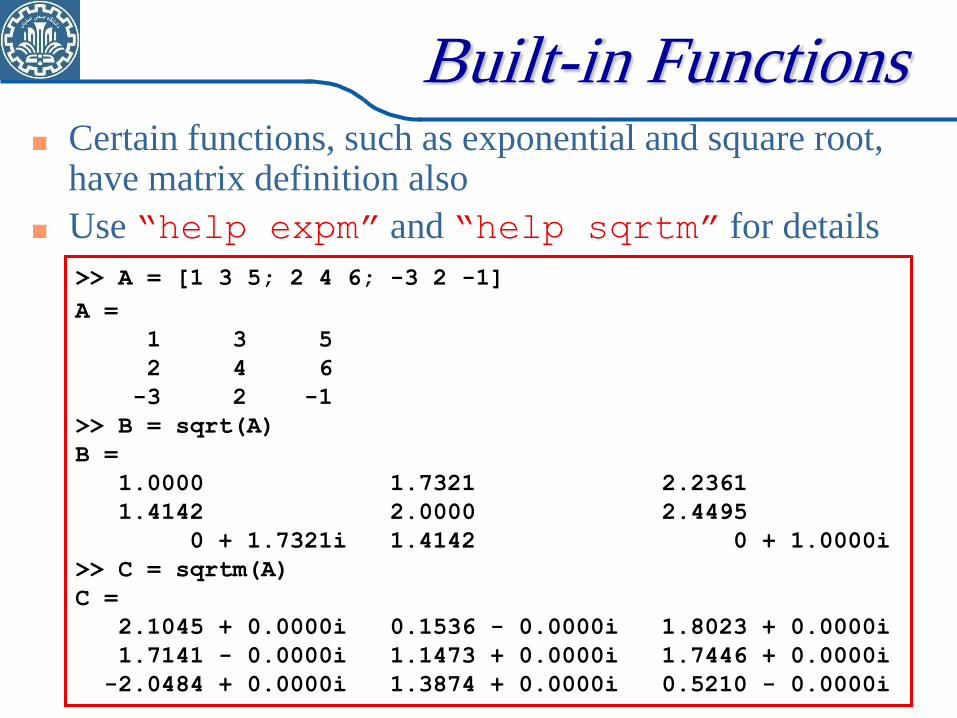
Built-in Functions Certain functions, such as exponential and square root,
have matrix definition also
Use “help expm” and “help sqrtm” for details
>> A = [1 3 5; 2 4 6; -3 2 -1]
A =
1 3 5
2 4 6
-3 2 -1
>> B = sqrt(A)
B =
1.0000 1.7321 2.2361
1.4142 2.0000 2.4495
0 + 1.7321i 1.4142 0 + 1.0000i
>> C = sqrtm(A)
C =
2.1045 + 0.0000i 0.1536 - 0.0000i 1.8023 + 0.0000i
1.7141 - 0.0000i 1.1473 + 0.0000i 1.7446 + 0.0000i
-2.0484 + 0.0000i 1.3874 + 0.0000i 0.5210 - 0.0000i
MATLAB Graphics
One of the best things about MATLAB is
interactive graphics
“plot” is the one you will be using most often
Many other 3D plotting functions -- plot3, mesh, surfc, etc.
Use “help plot” for plotting options
To get a new figure, use “figure”
logarithmic plots available using semilogx, semilogy and loglog
Plotting Commands
plot(x,y) defaults to a blue line
plot(x,y,‟ro‟) uses red circles
plot(x,y,‟g*‟) uses green asterisks
If you want to put two plots on the same graph,
use “hold on”
plot(a,b,‟r:‟) (red dotted line)
hold on
plot(a,c,‟ko‟) (black circles)
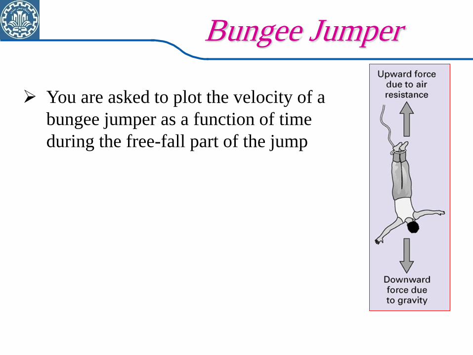
Bungee Jumper
You are asked to plot the velocity of a
bungee jumper as a function of time
during the free-fall part of the jump

Exact (Analytic) Solution
Newton’s Second Law
2d
2
d
vm
cg
dt
dv
vcmgdt
dvm
Exact Solution
t
m
gc
c
mgtv d
d
tanh)(

Free-Falling Bungee Jumper
Use built-in functions sqrt & tanh
>> g = 9.81; m = 75.2; cd = 0.24;
>> t = 0:1:20
t =
Columns 1 through 15
0 1 2 3 4 5 6 7 8 9 10 11 12 13 14
Columns 16 through 21
15 16 17 18 19 20
>> v=sqrt(g*m/cd)*tanh(sqrt(g*cd/m)*t)
v =
Columns 1 through 9
0 9.7089 18.8400 26.9454 33.7794 39.2956 43.5937 46.8514 49.2692
Columns 10 through 18
51.0358 52.3119 53.2262 53.8772 54.3389 54.6653 54.8956 55.0579 55.1720
Columns 19 through 21
55.2523 55.3087 55.3484
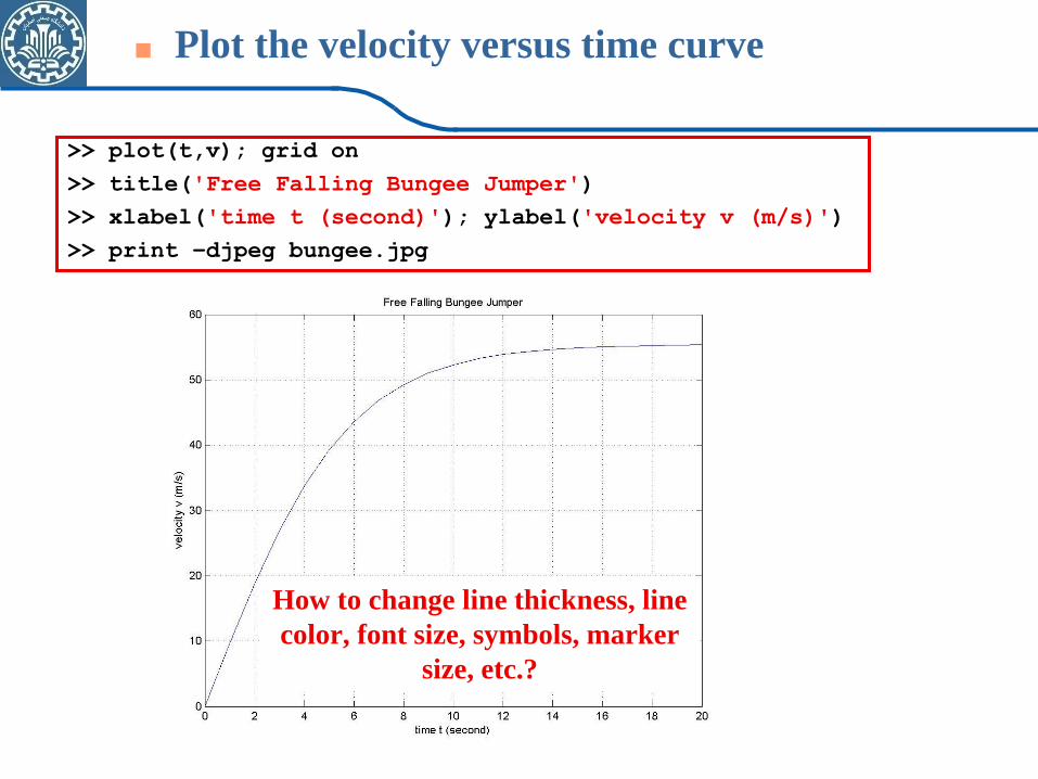
Plot the velocity versus time curve
>> plot(t,v); grid on
>> title('Free Falling Bungee Jumper')
>> xlabel('time t (second)'); ylabel('velocity v (m/s)')
>> print –djpeg bungee.jpg
How to change line thickness, line
color, font size, symbols, marker
size, etc.?
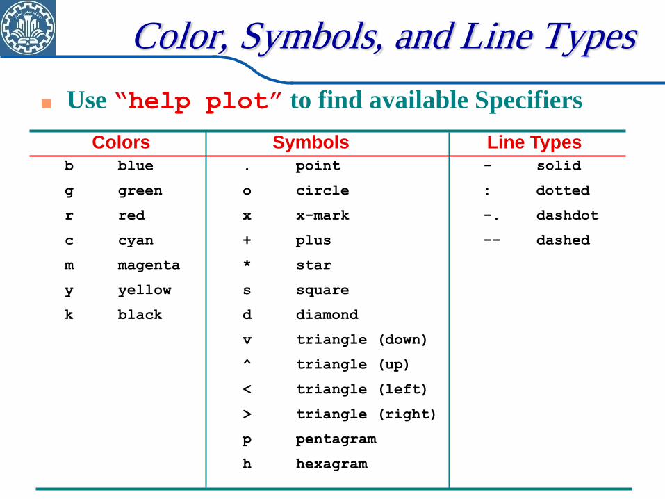
Color, Symbols, and Line Types
Use “help plot” to find available Specifiers
b blue . point - solid
g green o circle : dotted
r red x x-mark -. dashdot
c cyan + plus -- dashed
m magenta * star
y yellow s square
k black d diamond
v triangle (down)
^ triangle (up)
< triangle (left)
> triangle (right)
p pentagram
h hexagram
Colors Symbols Line Types
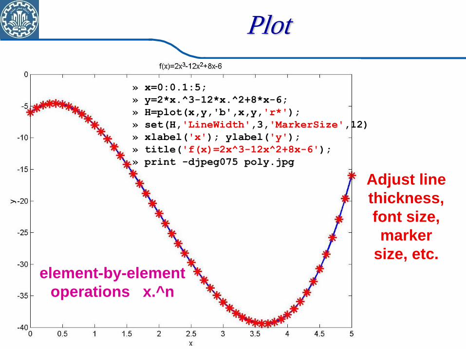
» x=0:0.1:5;
» y=2*x.^3-12*x.^2+8*x-6;
» H=plot(x,y,'b',x,y,'r*');
» set(H,'LineWidth',3,'MarkerSize',12)
» xlabel('x'); ylabel('y');
» title('f(x)=2x^3-12x^2+8x-6');
» print -djpeg075 poly.jpg
element-by-element
operations x.^n
Adjust line
thickness,
font size,
marker
size, etc.
Plot

» x=0:0.1:10; » y=sin(2.*pi*x)+cos(pi*x); » H1=plot(x,y,'m'); set(H1,'LineWidth',3); hold on; » H2=plot(x,y,'bO'); set(H2,'LineWidth',3,'MarkerSize',10); hold off; » xlabel('x'); ylabel('y'); » title('y = sin(2\pix)+cos(\pix)'); » print -djpeg075 function.jpg
Plot
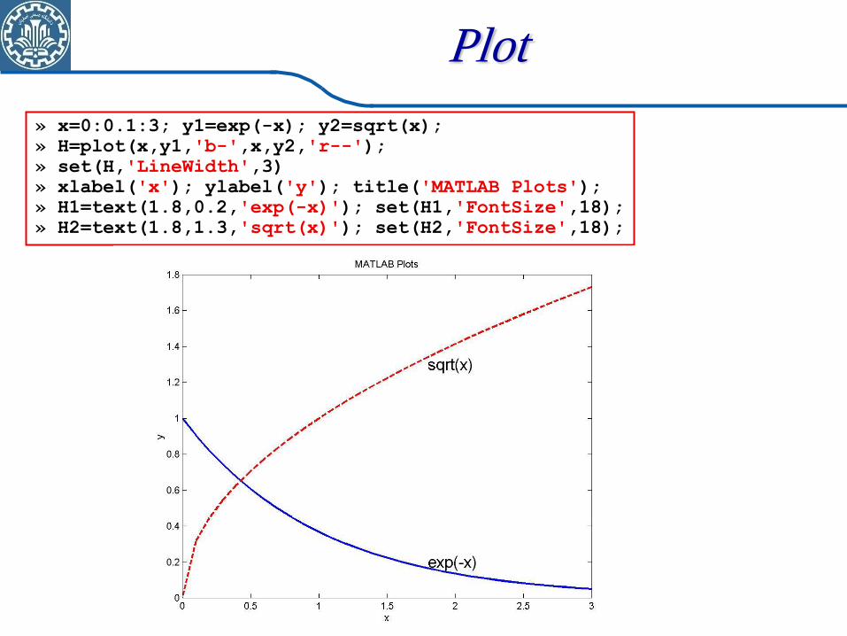
» x=0:0.1:3; y1=exp(-x); y2=sqrt(x);
» H=plot(x,y1,'b-',x,y2,'r--');
» set(H,'LineWidth',3)
» xlabel('x'); ylabel('y'); title('MATLAB Plots');
» H1=text(1.8,0.2,'exp(-x)'); set(H1,'FontSize',18);
» H2=text(1.8,1.3,'sqrt(x)'); set(H2,'FontSize',18);
Plot
Plotting Commands
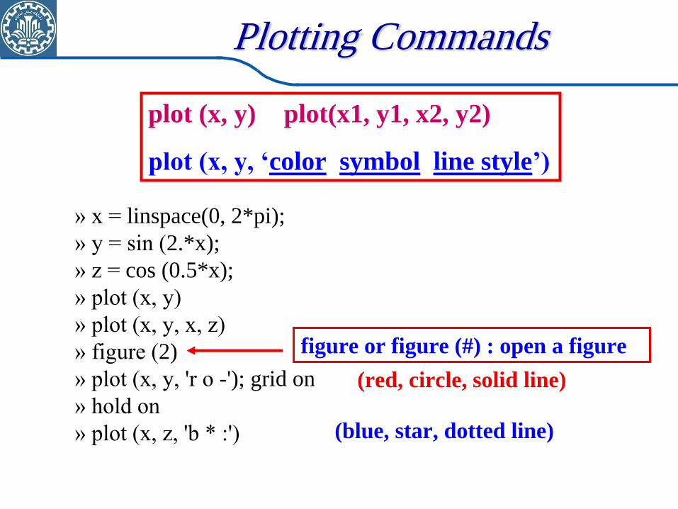
plot (x, y) plot(x1, y1, x2, y2)
plot (x, y, ‘color symbol line style’)
» x = linspace(0, 2*pi);
» y = sin (2.*x);
» z = cos (0.5*x);
» plot (x, y)
» plot (x, y, x, z)
» figure (2)
» plot (x, y, 'r o -'); grid on
» hold on
» plot (x, z, 'b * :')
(red, circle, solid line)
(blue, star, dotted line)
figure or figure (#) : open a figure
Graphics Commands
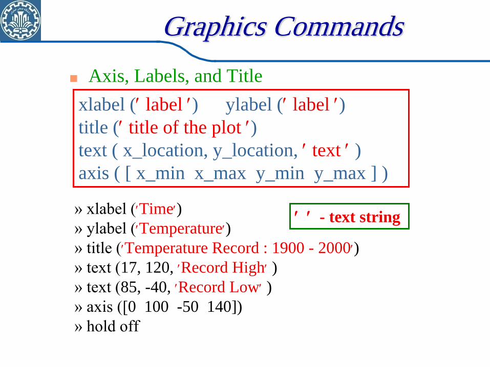
» xlabel (Time)
» ylabel (Temperature)
» title (Temperature Record : 1900 - 2000)
» text (17, 120, Record High )
» text (85, -40, Record Low )
» axis ([0 100 -50 140])
» hold off
xlabel ( label ) ylabel ( label )
title ( title of the plot )
text ( x_location, y_location, text )
axis ( [ x_min x_max y_min y_max ] )
- text string
Axis, Labels, and Title
Programming with
MATLAB
M-Files: Scripts and Functions
You can create and save code in text files using
MATLAB Editor/Debugger or other text editors
(called m-files since the ending must be .m)
M-file is an ASCII text file similar to FORTRAN or
C source codes ( computer programs)
A script can be executed by typing the file name, or
using the “run” command
Difference between scripts and functions
Scripts share variables with the main workspace
Functions do not
Script Files
Script file – a series of MATLAB commands
saved on a file, can be executed by
typing the file name in the Command Window
invoking the menu selections in the Edit Window: Debug, Run
Create a script file using menu selection:
File, New, M-file
Function File
Function file: M-file that starts with the word function
Function can accept input arguments and return outputs
Analogous to user-defined functions in programming languages such as Fortran, C, …
Save the function file as function_name.m
User help function in command window for additional information
Functions
One variable
function y = function_name(input arguments)
More than one output variables
function [y, z] = function_name(input arguments)
Examples: function y = my_func (x)
y = x^3 + 3*x^2 -5 * x +2 ;
function area = integral (f, a, b)
ya = feval (f, a); yb = feval(f, b);
area = (b-a)*(ya+yb)/2;
Functions
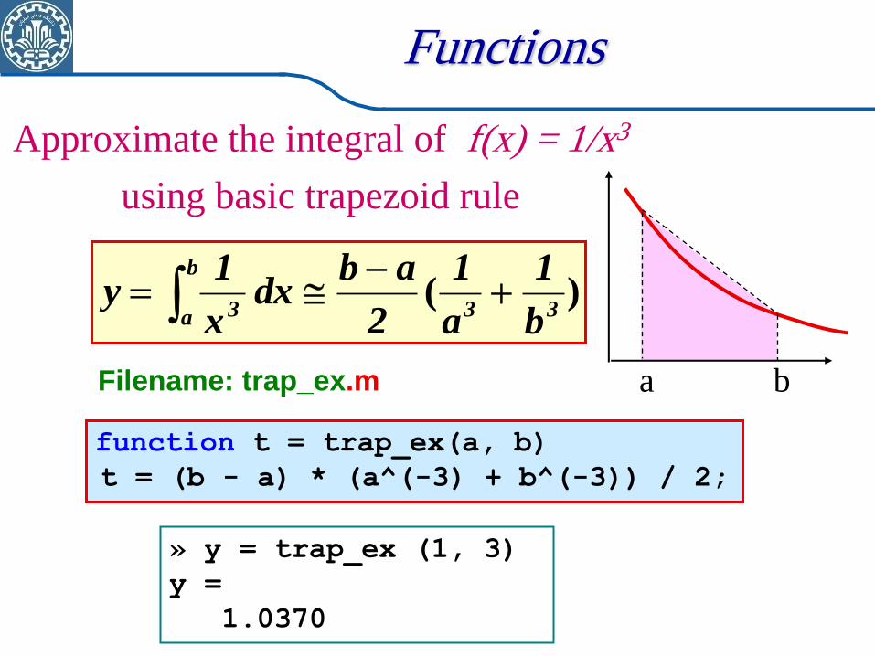
function t = trap_ex(a, b)
t = (b - a) * (a^(-3) + b^(-3)) / 2;
Approximate the integral of f(x) = 1/x3
using basic trapezoid rule
Filename: trap_ex.m
» y = trap_ex (1, 3)
y =
1.0370
)(
33
b
a 3 b
1
a
1
2
abdx
x
1y
a b
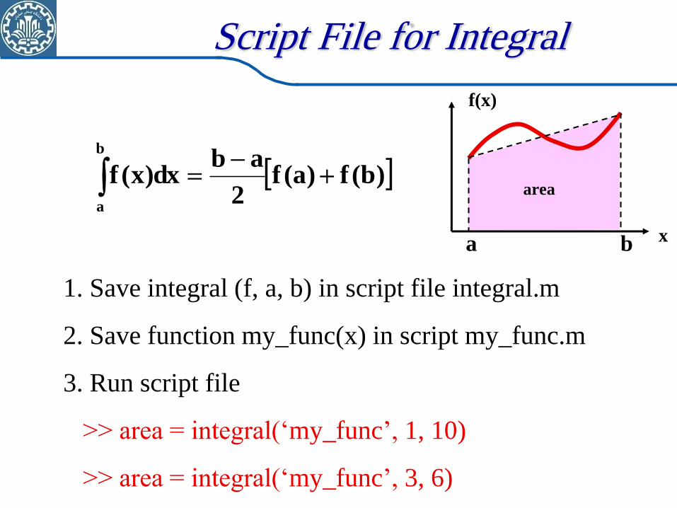
Script File for Integral
)b(f)a(f2
abdx)x(f
b
a
1. Save integral (f, a, b) in script file integral.m
2. Save function my_func(x) in script my_func.m
3. Run script file
>> area = integral(„my_func‟, 1, 10)
>> area = integral(„my_func‟, 3, 6)
area
a b
f(x)
x
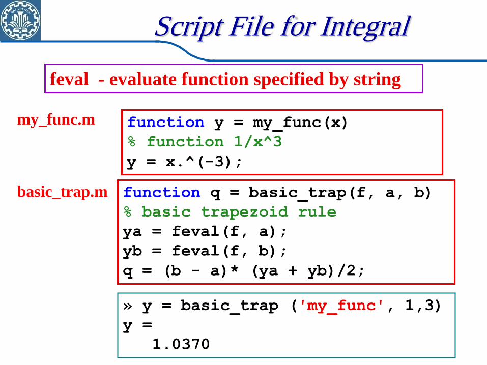
feval - evaluate function specified by string
function y = my_func(x)
% function 1/x^3
y = x.^(-3);
function q = basic_trap(f, a, b)
% basic trapezoid rule
ya = feval(f, a);
yb = feval(f, b);
q = (b - a)* (ya + yb)/2;
my_func.m
basic_trap.m
» y = basic_trap ('my_func', 1,3)
y =
1.0370
Script File for Integral
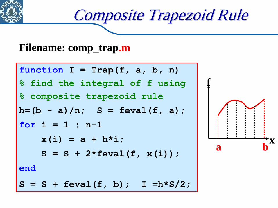
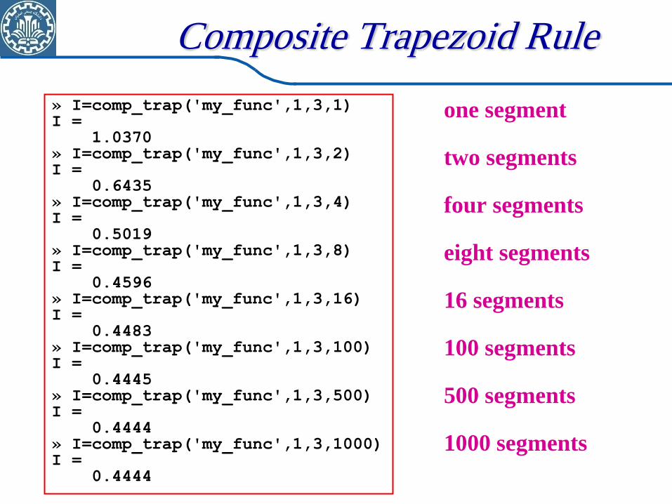
Composite Trapezoid Rule
function I = Trap(f, a, b, n)
% find the integral of f using
% composite trapezoid rule
h=(b - a)/n; S = feval(f, a);
for i = 1 : n-1
x(i) = a + h*i;
S = S + 2*feval(f, x(i));
end
S = S + feval(f, b); I =h*S/2;
Filename: comp_trap.m
x
f
a b
Composite Trapezoid Rule
» I=comp_trap('my_func',1,3,1) I = 1.0370 » I=comp_trap('my_func',1,3,2) I = 0.6435 » I=comp_trap('my_func',1,3,4) I = 0.5019 » I=comp_trap('my_func',1,3,8) I = 0.4596 » I=comp_trap('my_func',1,3,16) I = 0.4483 » I=comp_trap('my_func',1,3,100) I = 0.4445 » I=comp_trap('my_func',1,3,500) I = 0.4444 » I=comp_trap('my_func',1,3,1000) I = 0.4444
one segment
two segments
four segments
eight segments
16 segments
100 segments
500 segments
1000 segments
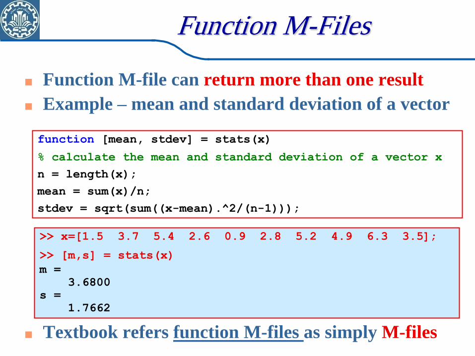
Function M-Files
Function M-file can return more than one result
Example – mean and standard deviation of a vector
Textbook refers function M-files as simply M-files
function [mean, stdev] = stats(x)
% calculate the mean and standard deviation of a vector x
n = length(x);
mean = sum(x)/n;
stdev = sqrt(sum((x-mean).^2/(n-1)));
>> x=[1.5 3.7 5.4 2.6 0.9 2.8 5.2 4.9 6.3 3.5];
>> [m,s] = stats(x)
m =
3.6800
s =
1.7662
Data Files
MAT Files -- memory efficient binary format
-- preferable for internal use by MATLAB program
ASCII files -- in ASCII characters
-- useful if the data is to be shared (imported or exported to other programs)
MATLAB Input
To read files in
if the file is an ascii table, use “load”
if the file is ascii but not a table, file I/O needs
“fopen” and “fclose”
Reading in data from file using fopen depends
on type of data (binary or text)
Default data type is “binary”
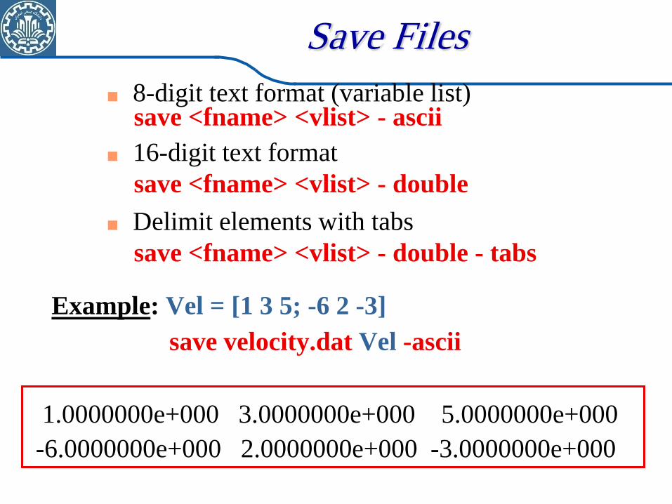
Save Files
8-digit text format (variable list) save <fname> <vlist> - ascii
16-digit text format
save <fname> <vlist> - double
Delimit elements with tabs
save <fname> <vlist> - double - tabs
Example: Vel = [1 3 5; -6 2 -3]
save velocity.dat Vel -ascii
1.0000000e+000 3.0000000e+000 5.0000000e+000
-6.0000000e+000 2.0000000e+000 -3.0000000e+000
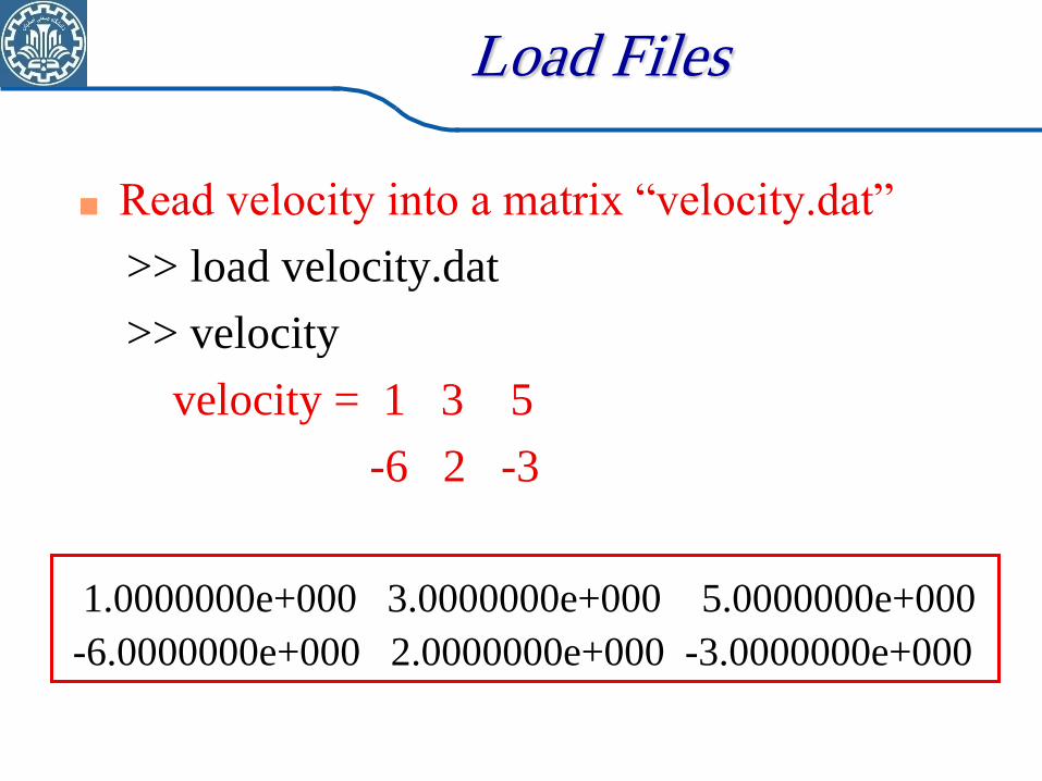
Load Files
Read velocity into a matrix “velocity.dat”
>> load velocity.dat
>> velocity
velocity = 1 3 5
-6 2 -3
1.0000000e+000 3.0000000e+000 5.0000000e+000
-6.0000000e+000 2.0000000e+000 -3.0000000e+000
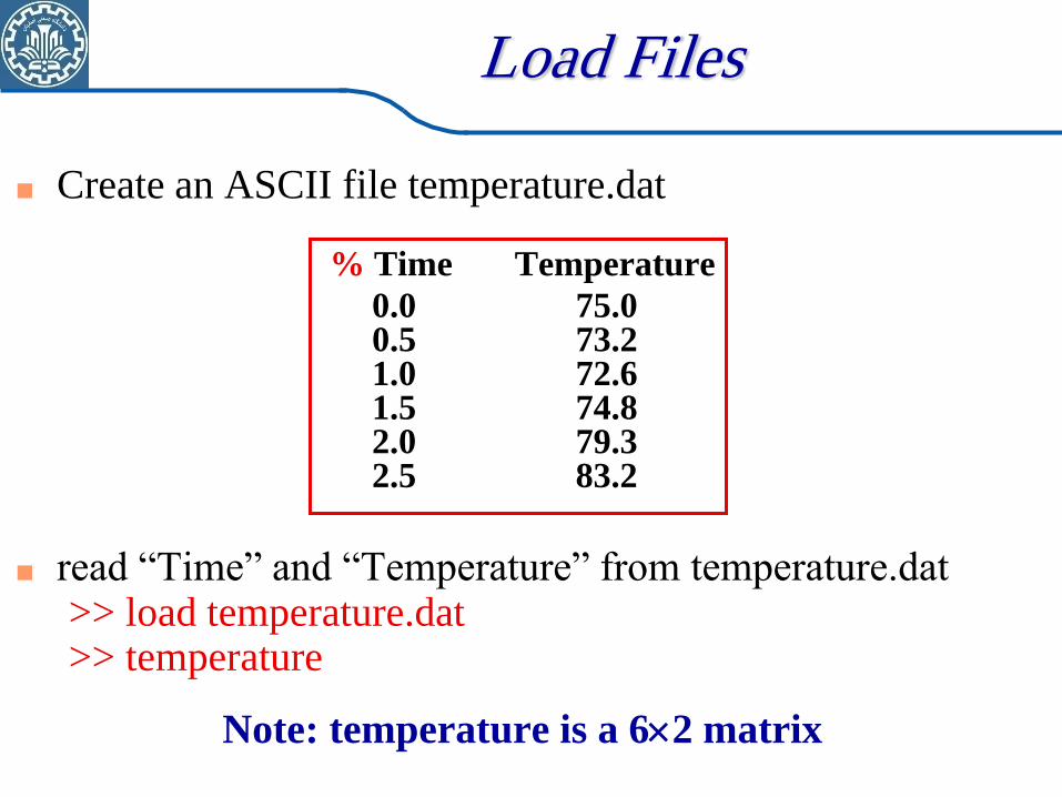
Load Files
Create an ASCII file temperature.dat
read “Time” and “Temperature” from temperature.dat >> load temperature.dat >> temperature
% Time Temperature
0.0 75.0 0.5 73.2 1.0 72.6 1.5 74.8 2.0 79.3 2.5 83.2
Note: temperature is a 62 matrix
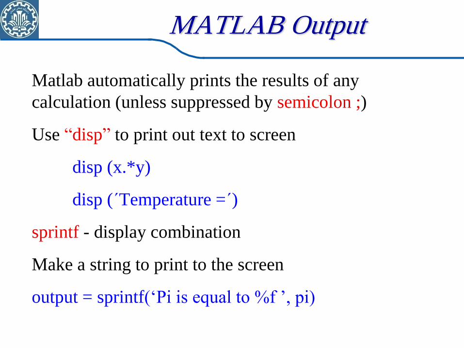
MATLAB Output
Matlab automatically prints the results of any
calculation (unless suppressed by semicolon ;)
Use “disp” to print out text to screen
disp (x.*y)
disp (´Temperature =´)
sprintf - display combination
Make a string to print to the screen
output = sprintf(„Pi is equal to %f ‟, pi)
Formatted Output
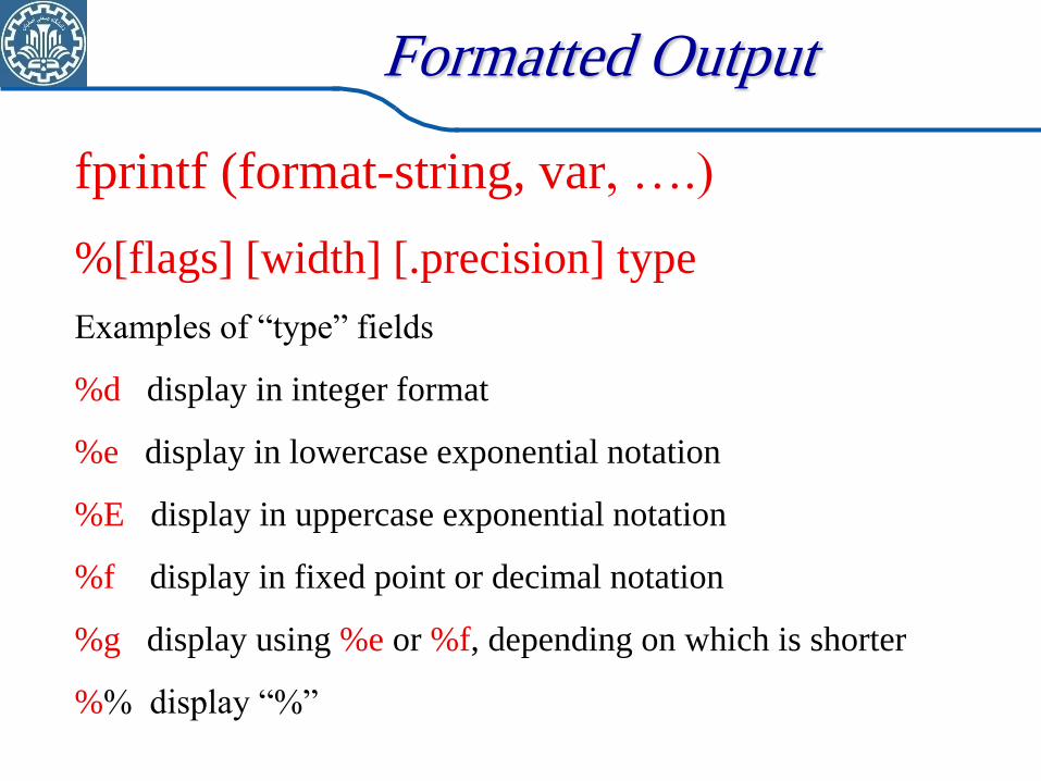
fprintf (format-string, var, ….)
%[flags] [width] [.precision] type
Examples of “type” fields
%d display in integer format
%e display in lowercase exponential notation
%E display in uppercase exponential notation
%f display in fixed point or decimal notation
%g display using %e or %f, depending on which is shorter
%% display “%”
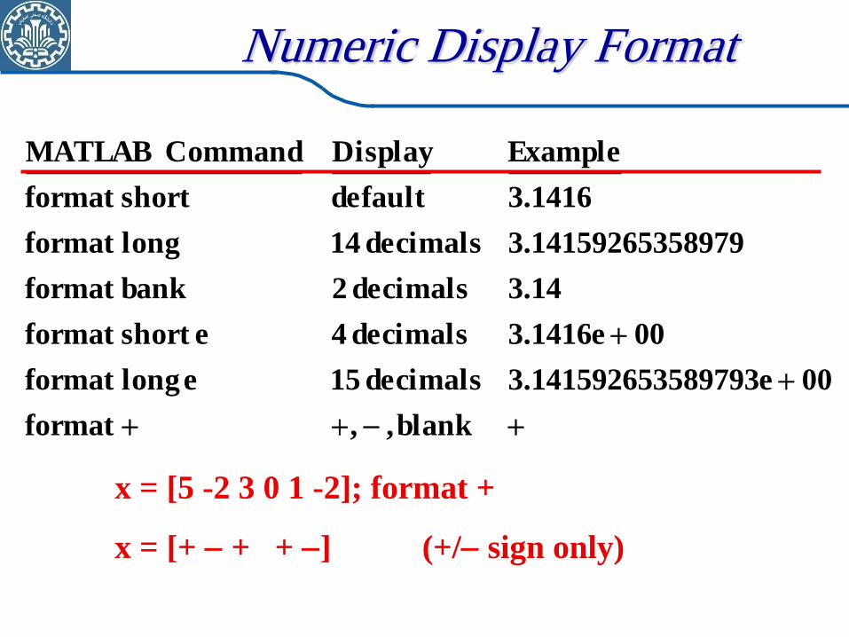
Numeric Display Format
blank, ,format
00e897931415926535.3decimals 15e longformat
00e1416.3decimals 4eshort format
14.3decimals 2bankformat
89791415926535.3decimals 14longformat
1416.3defaultshortformat
ExampleDisplayCommand MATLAB
x = [5 -2 3 0 1 -2]; format +
x = [+ + + ] (+/ sign only)
Programming
Selection (IF) Statements
The most common form of selection structure is
simple if statement
The if statement will have a condition associated
with it
The condition is typically a logical expression that
must be evaluated as either “true” or “false”
The outcome of the evaluation will determine the
next step performed
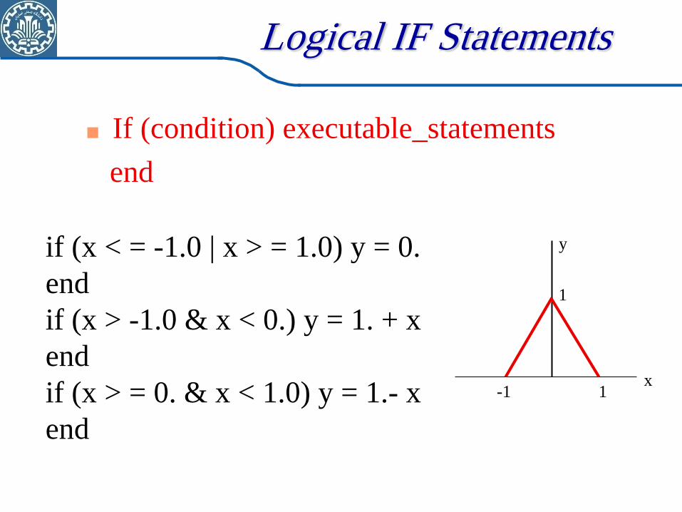
Logical IF Statements
If (condition) executable_statements
end
if (x < = -1.0 | x > = 1.0) y = 0.
end
if (x > -1.0 & x < 0.) y = 1. + x
end
if (x > = 0. & x < 1.0) y = 1.- x
end
-1 1 x
1
y
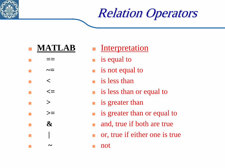
Relation Operators
Interpretation
is equal to
is not equal to
is less than
is less than or equal to
is greater than
is greater than or equal to
and, true if both are true
or, true if either one is true
not
MATLAB
==
~=
<
<=
>
>=
&
|
~
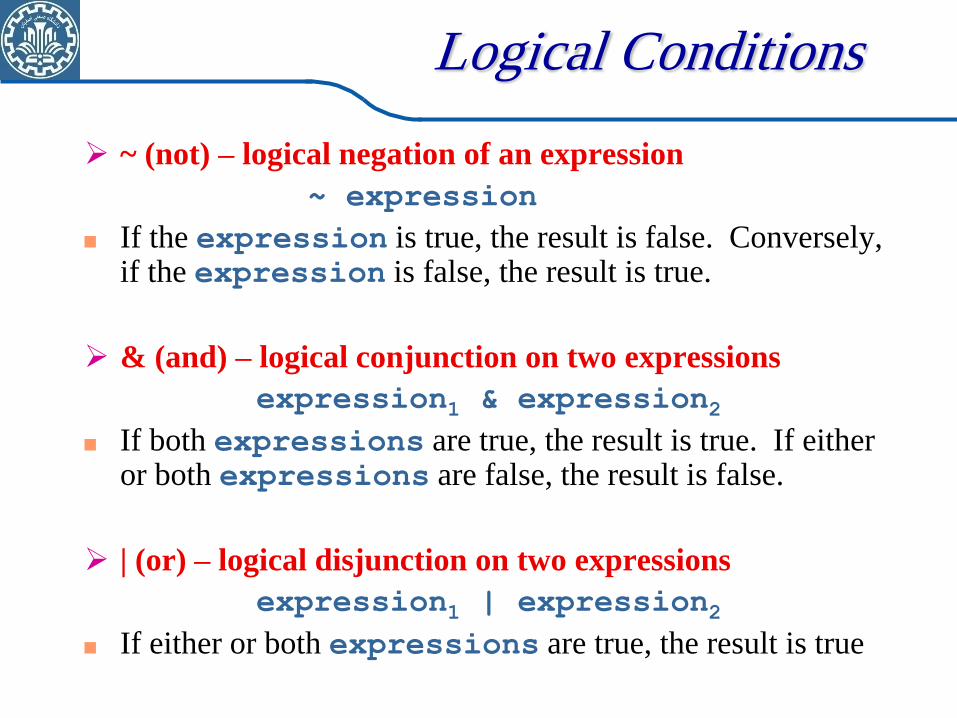
Logical Conditions
~ (not) – logical negation of an expression
~ expression
If the expression is true, the result is false. Conversely, if the expression is false, the result is true.
& (and) – logical conjunction on two expressions
expression1 & expression2
If both expressions are true, the result is true. If either or both expressions are false, the result is false.
| (or) – logical disjunction on two expressions
expression1 | expression2
If either or both expressions are true, the result is true
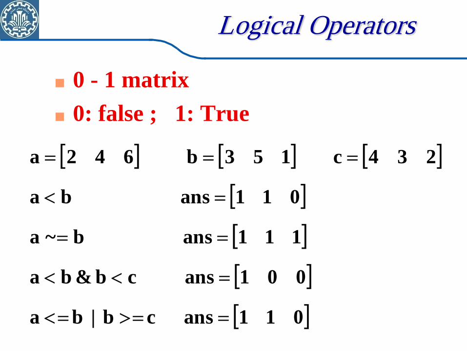
Logical Operators
0 - 1 matrix
0: false ; 1: True
011ans cb | ba
001ans cb & ba
111ans b~a
011ans ba
234c 153b 642a
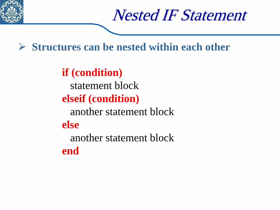
Nested IF Statement
if (condition)
statement block
elseif (condition)
another statement block
else
another statement block
end
Structures can be nested within each other
How to use Nested IF
If the condition is true the statements
following the statement block are
executed.
If the condition is not true, then the
control is transferred to the next
else, elseif, or end statement at the same if
level.
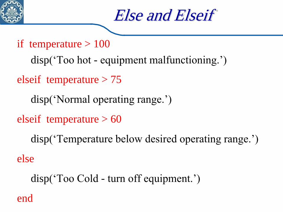
Else and Elseif
if temperature > 100
disp(„Too hot - equipment malfunctioning.‟)
elseif temperature > 75
disp(„Normal operating range.‟)
elseif temperature > 60
disp(„Temperature below desired operating range.‟)
else
disp(„Too Cold - turn off equipment.‟)
end
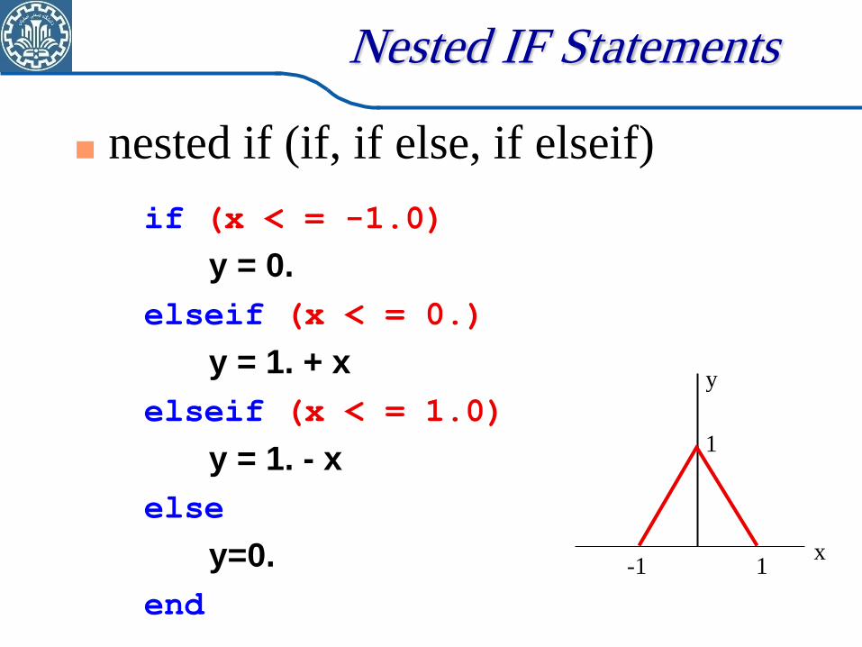
Nested IF Statements
if (x < = -1.0)
y = 0.
elseif (x < = 0.)
y = 1. + x
elseif (x < = 1.0)
y = 1. - x
else
y=0.
end
nested if (if, if else, if elseif)
-1 1 x
1
y
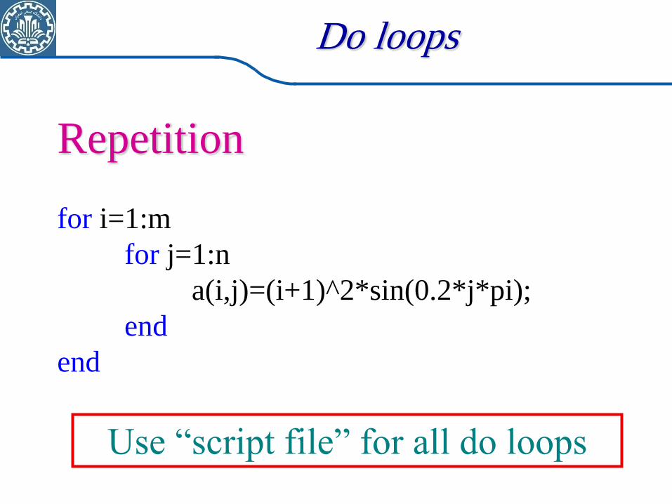
Do loops
Repetition
for i=1:m
for j=1:n
a(i,j)=(i+1)^2*sin(0.2*j*pi);
end
end
Use “script file” for all do loops
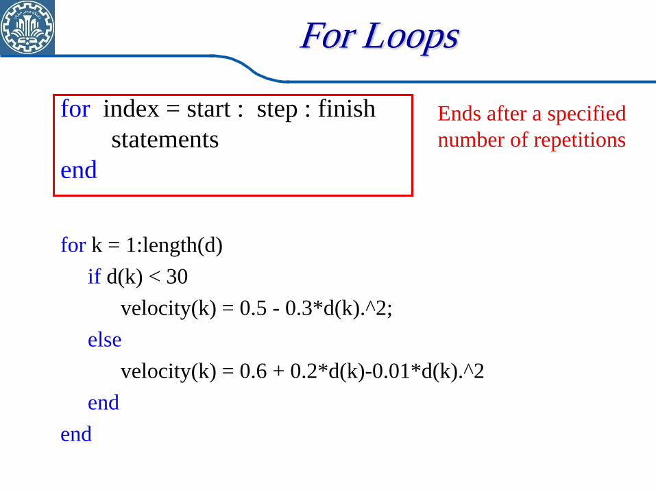
For Loops
for index = start : step : finish
statements
end
for k = 1:length(d)
if d(k) < 30
velocity(k) = 0.5 - 0.3*d(k).^2;
else
velocity(k) = 0.6 + 0.2*d(k)-0.01*d(k).^2
end
end
Ends after a specified
number of repetitions
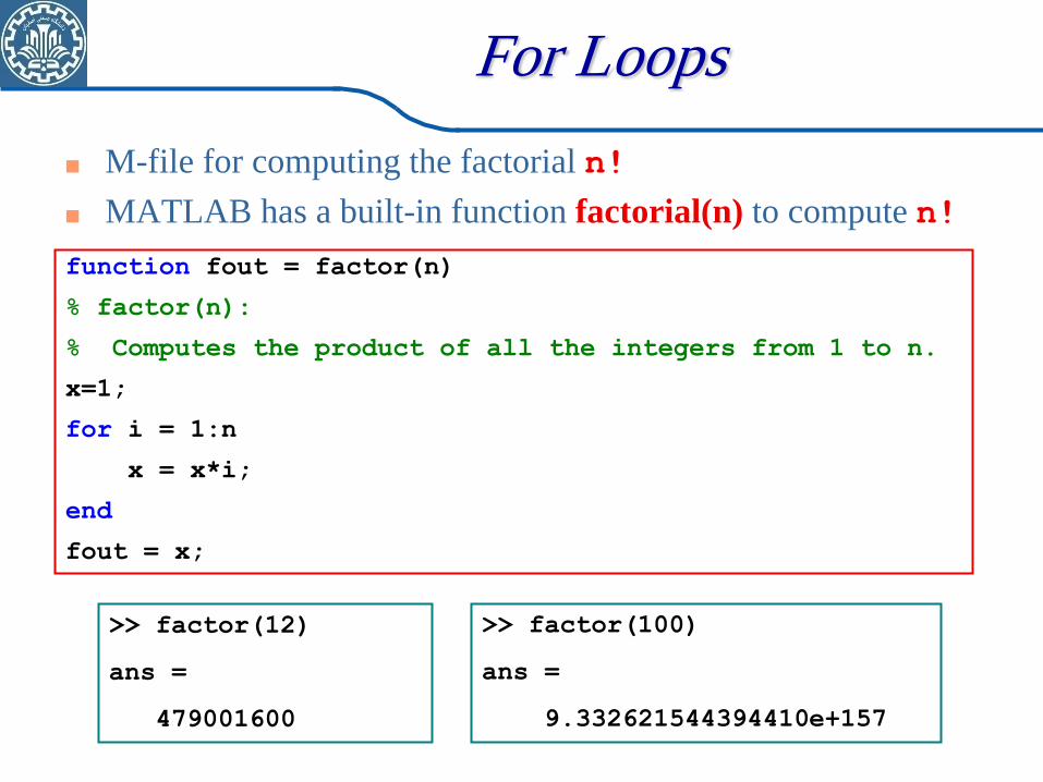
For Loops
M-file for computing the factorial n!
MATLAB has a built-in function factorial(n) to compute n!
function fout = factor(n)
% factor(n):
% Computes the product of all the integers from 1 to n.
x=1;
for i = 1:n
x = x*i;
end
fout = x;
>> factor(12)
ans =
479001600
>> factor(100)
ans =
9.332621544394410e+157
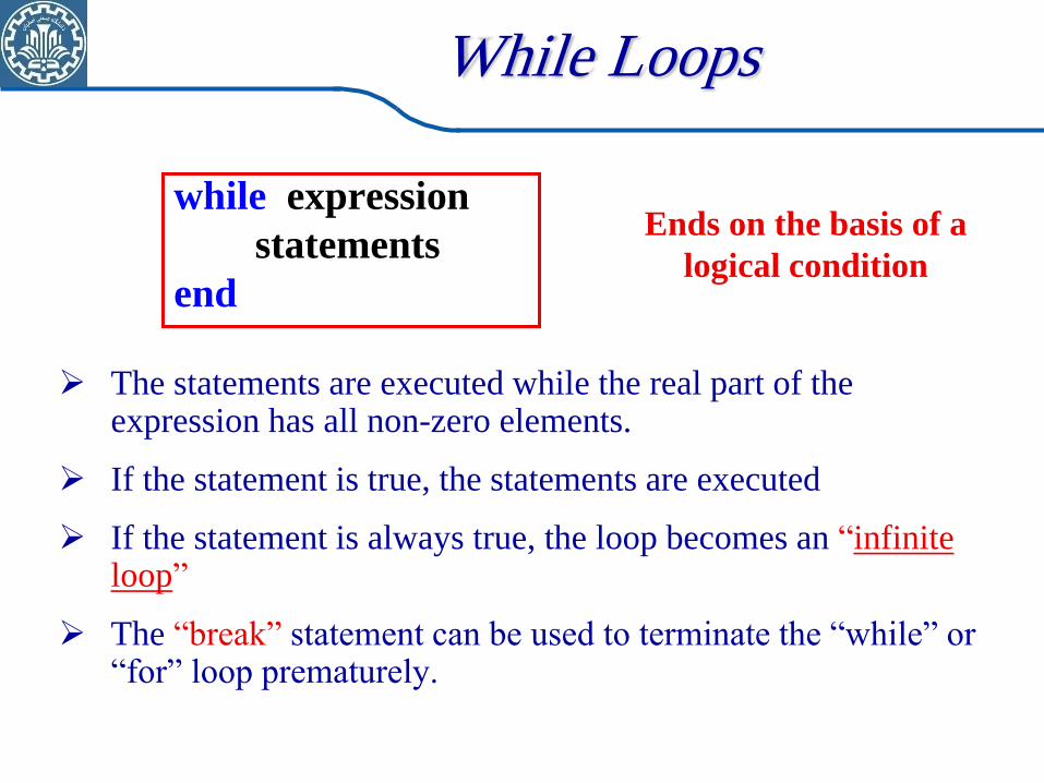
While Loops
while expression
statements
end
Ends on the basis of a
logical condition
The statements are executed while the real part of the expression has all non-zero elements.
If the statement is true, the statements are executed
If the statement is always true, the loop becomes an “infinite loop”
The “break” statement can be used to terminate the “while” or “for” loop prematurely.
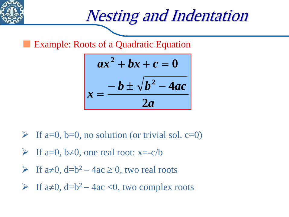
Nesting and Indentation
Example: Roots of a Quadratic Equation
a
acbbx
cbxax
2
4
0
2
2
If a=0, b=0, no solution (or trivial sol. c=0)
If a=0, b0, one real root: x=-c/b
If a0, d=b2 4ac 0, two real roots
If a0, d=b2 4ac <0, two complex roots
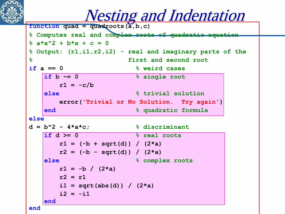
Nesting and Indentation function quad = quadroots(a,b,c)
% Computes real and complex roots of quadratic equation
% a*x^2 + b*x + c = 0
% Output: (r1,i1,r2,i2) - real and imaginary parts of the
% first and second root
if a == 0 % weird cases
if b ~= 0 % single root
r1 = -c/b
else % trivial solution
error('Trivial or No Solution. Try again')
end % quadratic formula
else
d = b^2 - 4*a*c; % discriminant
if d >= 0 % real roots
r1 = (-b + sqrt(d)) / (2*a)
r2 = (-b - sqrt(d)) / (2*a)
else % complex roots
r1 = -b / (2*a)
r2 = r1
i1 = sqrt(abs(d)) / (2*a)
i2 = -i1
end
end
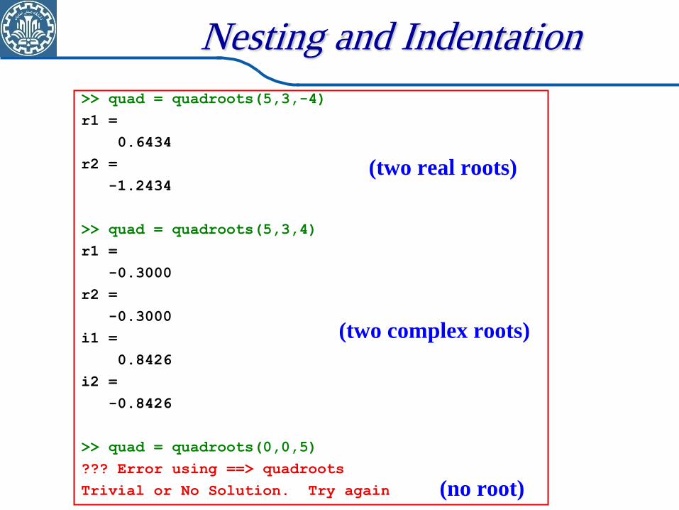
Nesting and Indentation
>> quad = quadroots(5,3,-4)
r1 =
0.6434
r2 =
-1.2434
>> quad = quadroots(5,3,4)
r1 =
-0.3000
r2 =
-0.3000
i1 =
0.8426
i2 =
-0.8426
>> quad = quadroots(0,0,5)
??? Error using ==> quadroots
Trivial or No Solution. Try again
(two real roots)
(two complex roots)
(no root)
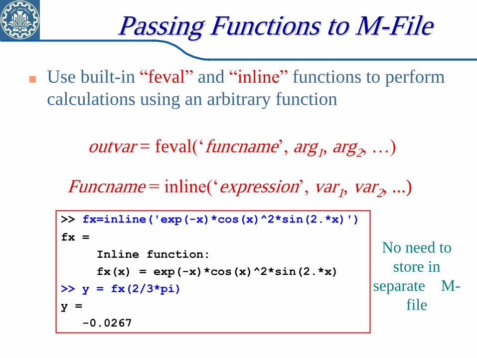
Passing Functions to M-File
Use built-in “feval” and “inline” functions to perform
calculations using an arbitrary function
outvar = feval(„funcname‟, arg1, arg2, …)
Funcname = inline(„expression‟, var1, var2, ...)
>> fx=inline('exp(-x)*cos(x)^2*sin(2.*x)')
fx =
Inline function:
fx(x) = exp(-x)*cos(x)^2*sin(2.*x)
>> y = fx(2/3*pi)
y =
-0.0267
No need to
store in
separate M-
file

Summary
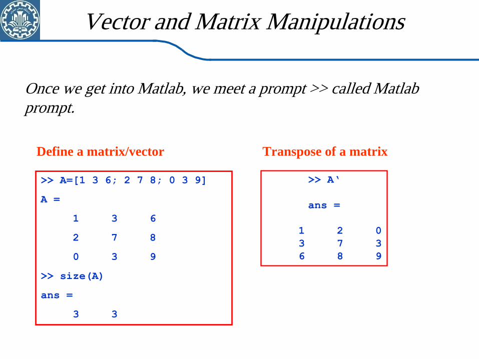
>> A=[1 3 6; 2 7 8; 0 3 9]
A =
1 3 6
2 7 8
0 3 9
>> size(A)
ans =
3 3
Define a matrix/vector Transpose of a matrix
>> A„
ans =
1 2 0
3 7 3
6 8 9
Vector and Matrix Manipulations
Once we get into Matlab, we meet a prompt >> called Matlab
prompt.
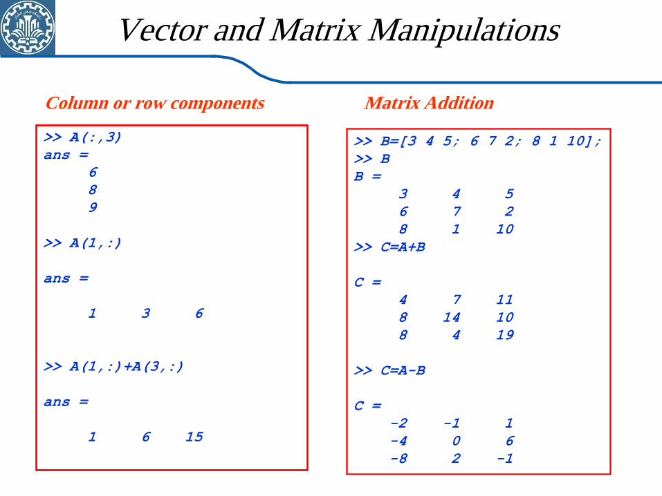
>> A(:,3)
ans =
6
8
9
>> A(1,:)
ans =
1 3 6
>> A(1,:)+A(3,:)
ans =
1 6 15
Column or row components
>> B=[3 4 5; 6 7 2; 8 1 10];
>> B
B =
3 4 5
6 7 2
8 1 10
>> C=A+B
C =
4 7 11
8 14 10
8 4 19
>> C=A-B
C =
-2 -1 1
-4 0 6
-8 2 -1
Vector and Matrix Manipulations
Matrix Addition
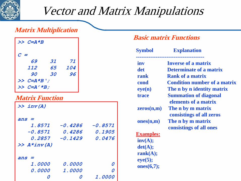
Matrix Multiplication
>> C=A*B
C =
69 31 71
112 65 104
90 30 96
>> C=A*B„;
>> C=A‟*B;
Vector and Matrix Manipulations
Basic matrix Functions
Matrix Function >> inv(A)
ans =
1.8571 -0.4286 -0.8571
-0.8571 0.4286 0.1905
0.2857 -0.1429 0.0476
>> A*inv(A)
ans =
1.0000 0.0000 0
0.0000 1.0000 0
0 0 1.0000
Symbol Explanation
--------------------------------------
inv Inverse of a matrix
det Determinate of a matrix
rank Rank of a matrix
cond Condition number of a matrix
eye(n) The n by n identity matrix
trace Summation of diagonal
elements of a matrix
zeros(n,m) The n by m matrix
consistings of all zeros
ones(n,m) The n by m matrix
consistings of all ones
Examples:
inv(A);
det(A);
rank(A);
eye(5);
ones(6,7);
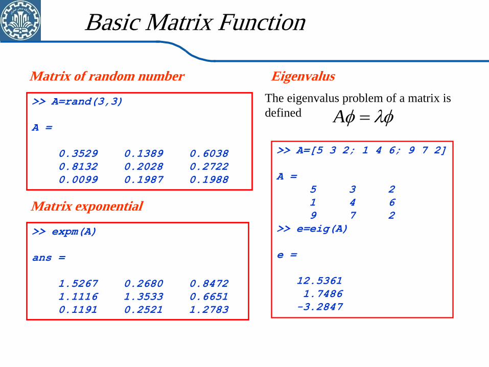
>> A=rand(3,3)
A =
0.3529 0.1389 0.6038
0.8132 0.2028 0.2722
0.0099 0.1987 0.1988
Matrix of random number
>> A=[5 3 2; 1 4 6; 9 7 2]
A =
5 3 2
1 4 6
9 7 2
>> e=eig(A)
e =
12.5361
1.7486
-3.2847
Basic Matrix Function
Eigenvalus
>> expm(A)
ans =
1.5267 0.2680 0.8472
1.1116 1.3533 0.6651
0.1191 0.2521 1.2783
Matrix exponential
AThe eigenvalus problem of a matrix is
defined
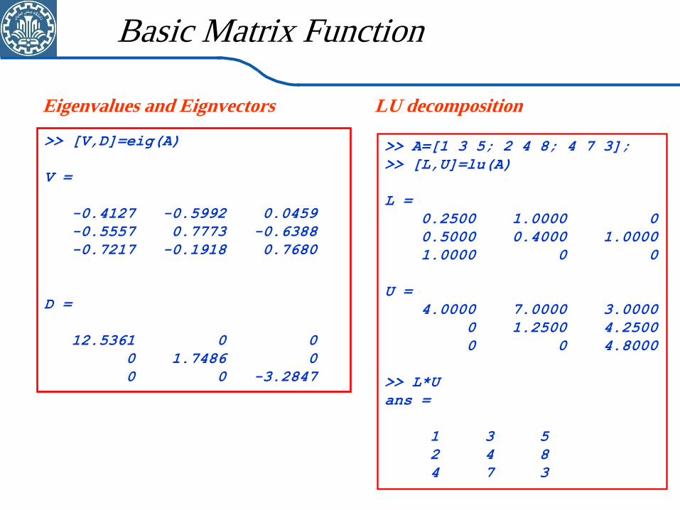
>> [V,D]=eig(A)
V =
-0.4127 -0.5992 0.0459
-0.5557 0.7773 -0.6388
-0.7217 -0.1918 0.7680
D =
12.5361 0 0
0 1.7486 0
0 0 -3.2847
Eigenvalues and Eignvectors
>> A=[1 3 5; 2 4 8; 4 7 3];
>> [L,U]=lu(A)
L =
0.2500 1.0000 0
0.5000 0.4000 1.0000
1.0000 0 0
U =
4.0000 7.0000 3.0000
0 1.2500 4.2500
0 0 4.8000
>> L*U
ans =
1 3 5
2 4 8
4 7 3
Basic Matrix Function
LU decomposition
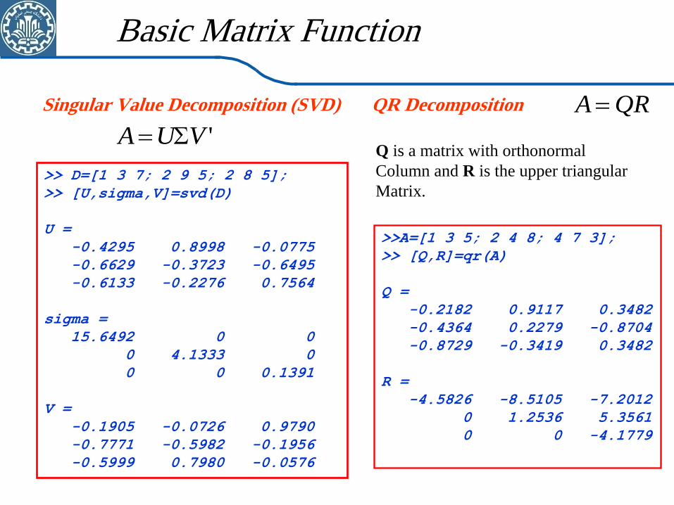
>> D=[1 3 7; 2 9 5; 2 8 5];
>> [U,sigma,V]=svd(D)
U =
-0.4295 0.8998 -0.0775
-0.6629 -0.3723 -0.6495
-0.6133 -0.2276 0.7564
sigma =
15.6492 0 0
0 4.1333 0
0 0 0.1391
V =
-0.1905 -0.0726 0.9790
-0.7771 -0.5982 -0.1956
-0.5999 0.7980 -0.0576
Singular Value Decomposition (SVD)
>>A=[1 3 5; 2 4 8; 4 7 3];
>> [Q,R]=qr(A)
Q =
-0.2182 0.9117 0.3482
-0.4364 0.2279 -0.8704
-0.8729 -0.3419 0.3482
R =
-4.5826 -8.5105 -7.2012
0 1.2536 5.3561
0 0 -4.1779
Basic Matrix Function
QR Decomposition
'VUA
QRA
Q is a matrix with orthonormal
Column and R is the upper triangular
Matrix.
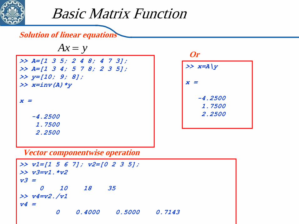
>> A=[1 3 5; 2 4 8; 4 7 3];
>> A=[1 3 4; 5 7 8; 2 3 5];
>> y=[10; 9; 8];
>> x=inv(A)*y
x =
-4.2500
1.7500
2.2500
Solution of linear equations
Basic Matrix Function
Ax y
>> x=A\y
x =
-4.2500
1.7500
2.2500
Or
Vector componentwise operation
>> v1=[1 5 6 7]; v2=[0 2 3 5];
>> v3=v1.*v2
v3 =
0 10 18 35
>> v4=v2./v1
v4 =
0 0.4000 0.5000 0.7143
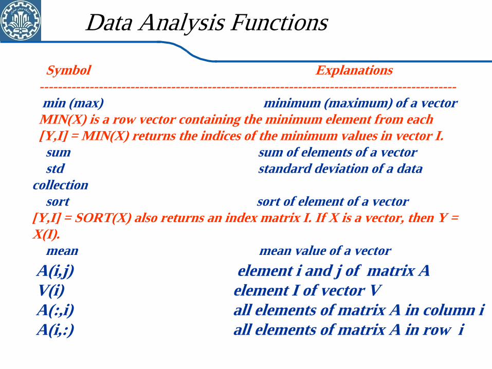
Symbol Explanations
--------------------------------------------------------------------------------------------
min (max) minimum (maximum) of a vector
MIN(X) is a row vector containing the minimum element from each
[Y,I] = MIN(X) returns the indices of the minimum values in vector I.
sum sum of elements of a vector
std standard deviation of a data
collection
sort sort of element of a vector
[Y,I] = SORT(X) also returns an index matrix I. If X is a vector, then Y =
X(I).
mean mean value of a vector
Data Analysis Functions
A(i,j) element i and j of matrix A
V(i) element I of vector V
A(:,i) all elements of matrix A in column i
A(i,:) all elements of matrix A in row i
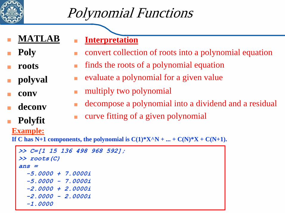
Interpretation
convert collection of roots into a polynomial equation
finds the roots of a polynomial equation
evaluate a polynomial for a given value
multiply two polynomial
decompose a polynomial into a dividend and a residual
curve fitting of a given polynomial
MATLAB
Poly
roots
polyval
conv
deconv
Polyfit
Polynomial Functions
Example: If C has N+1 components, the polynomial is C(1)*X^N + ... + C(N)*X + C(N+1).
>> C=[1 15 136 498 968 592];
>> roots(C)
ans =
-5.0000 + 7.0000i
-5.0000 - 7.0000i
-2.0000 + 2.0000i
-2.0000 - 2.0000i
-1.0000
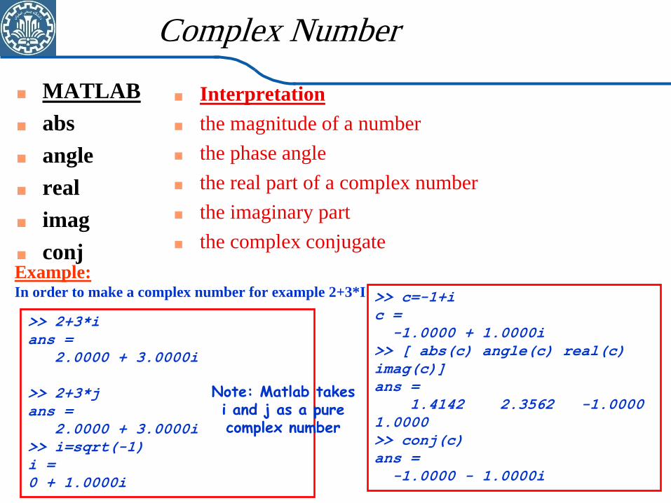
Interpretation
the magnitude of a number
the phase angle
the real part of a complex number
the imaginary part
the complex conjugate
MATLAB
abs
angle
real
imag
conj
Complex Number
Example: In order to make a complex number for example 2+3*I
>> 2+3*i
ans =
2.0000 + 3.0000i
>> 2+3*j
ans =
2.0000 + 3.0000i
>> i=sqrt(-1)
i =
0 + 1.0000i
>> c=-1+i
c =
-1.0000 + 1.0000i
>> [ abs(c) angle(c) real(c)
imag(c)]
ans =
1.4142 2.3562 -1.0000
1.0000
>> conj(c)
ans =
-1.0000 - 1.0000i
Note: Matlab takes i and j as a pure complex number
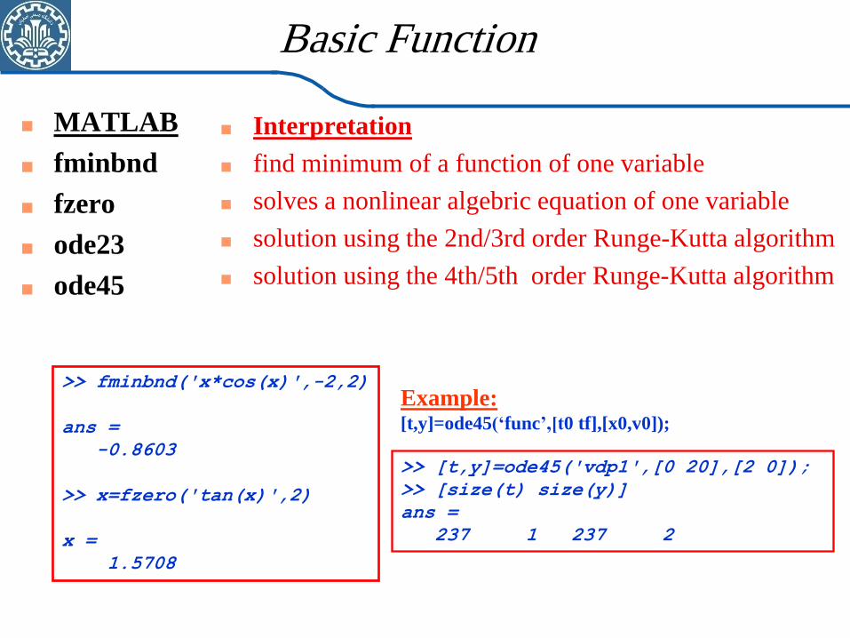
>> fminbnd('x*cos(x)',-2,2)
ans =
-0.8603
>> x=fzero('tan(x)',2)
x =
1.5708
>> [t,y]=ode45('vdp1',[0 20],[2 0]);
>> [size(t) size(y)]
ans =
237 1 237 2
Basic Function
Interpretation
find minimum of a function of one variable
solves a nonlinear algebric equation of one variable
solution using the 2nd/3rd order Runge-Kutta algorithm
solution using the 4th/5th order Runge-Kutta algorithm
MATLAB
fminbnd
fzero
ode23
ode45
Example: [t,y]=ode45(‘func’,[t0 tf],[x0,v0]);
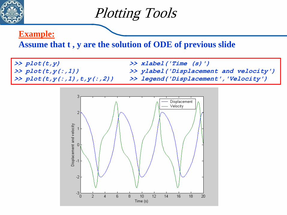
>> plot(t,y) >> xlabel('Time (s)')
>> plot(t,y(:,1)) >> ylabel('Displacement and velocity')
>> plot(t,y(:,1),t,y(:,2)) >> legend('Displacement','Velocity')
Plotting Tools
Example:
Assume that t , y are the solution of ODE of previous slide
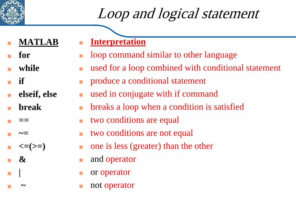
Loop and logical statement
Interpretation
loop command similar to other language
used for a loop combined with conditional statement
produce a conditional statement
used in conjugate with if command
breaks a loop when a condition is satisfied
two conditions are equal
two conditions are not equal
one is less (greater) than the other
and operator
or operator
not operator
MATLAB
for
while
if
elseif, else
break
==
~=
<=(>=)
&
|
~
Writing Function Subroutine
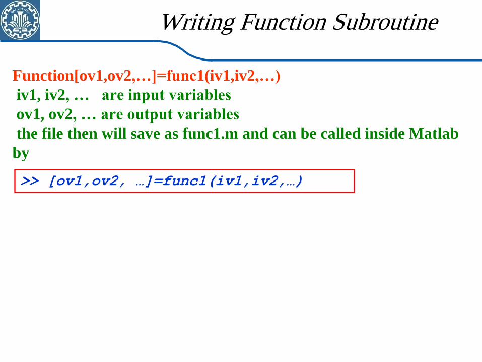
Function[ov1,ov2,…]=func1(iv1,iv2,…)
iv1, iv2, … are input variables
ov1, ov2, … are output variables
the file then will save as func1.m and can be called inside Matlab
by
>> [ov1,ov2, …]=func1(iv1,iv2,…)
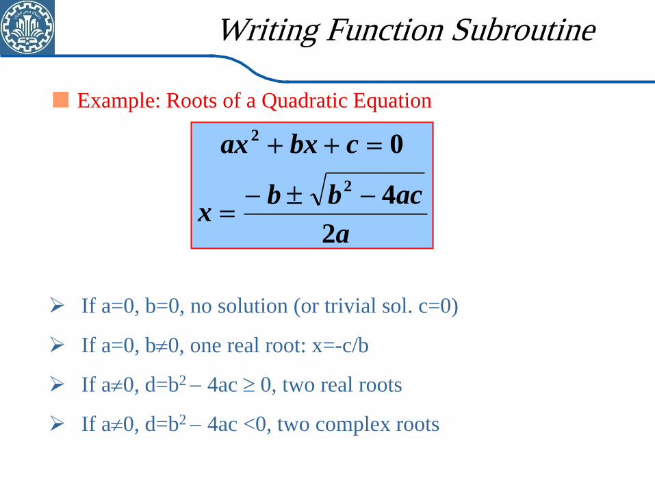
Example: Roots of a Quadratic Equation
a
acbbx
cbxax
2
4
0
2
2
If a=0, b=0, no solution (or trivial sol. c=0)
If a=0, b0, one real root: x=-c/b
If a0, d=b2 4ac 0, two real roots
If a0, d=b2 4ac <0, two complex roots
Writing Function Subroutine
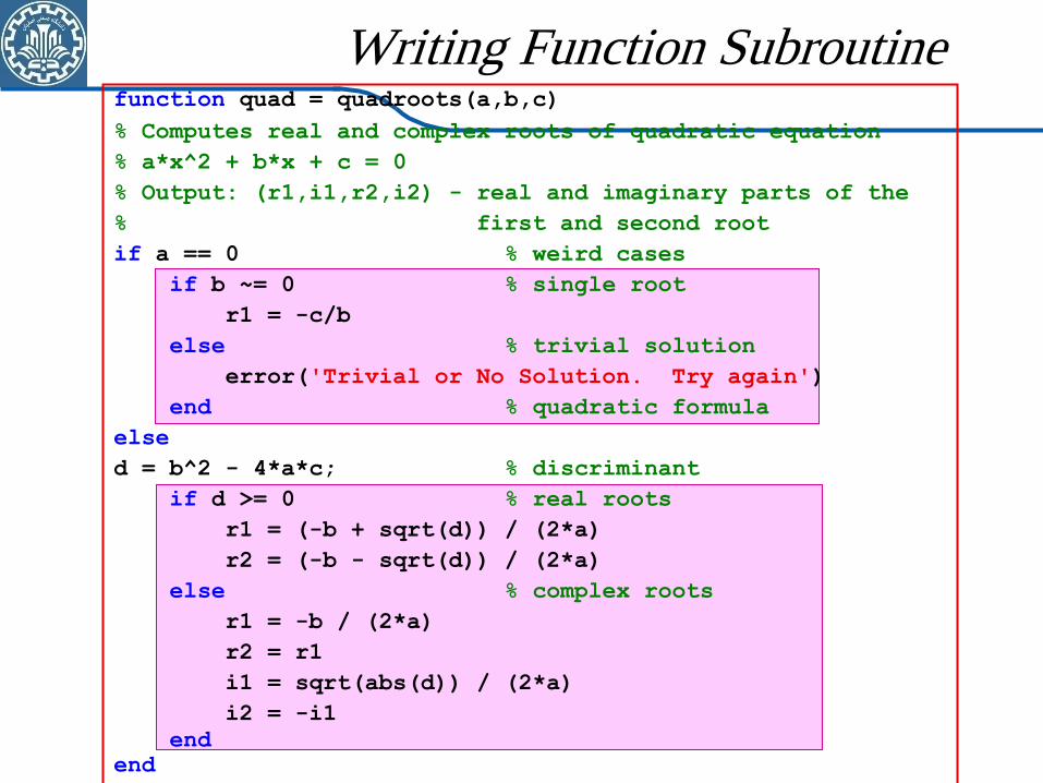
function quad = quadroots(a,b,c)
% Computes real and complex roots of quadratic equation
% a*x^2 + b*x + c = 0
% Output: (r1,i1,r2,i2) - real and imaginary parts of the
% first and second root
if a == 0 % weird cases
if b ~= 0 % single root
r1 = -c/b
else % trivial solution
error('Trivial or No Solution. Try again')
end % quadratic formula
else
d = b^2 - 4*a*c; % discriminant
if d >= 0 % real roots
r1 = (-b + sqrt(d)) / (2*a)
r2 = (-b - sqrt(d)) / (2*a)
else % complex roots
r1 = -b / (2*a)
r2 = r1
i1 = sqrt(abs(d)) / (2*a)
i2 = -i1
end
end
Writing Function Subroutine
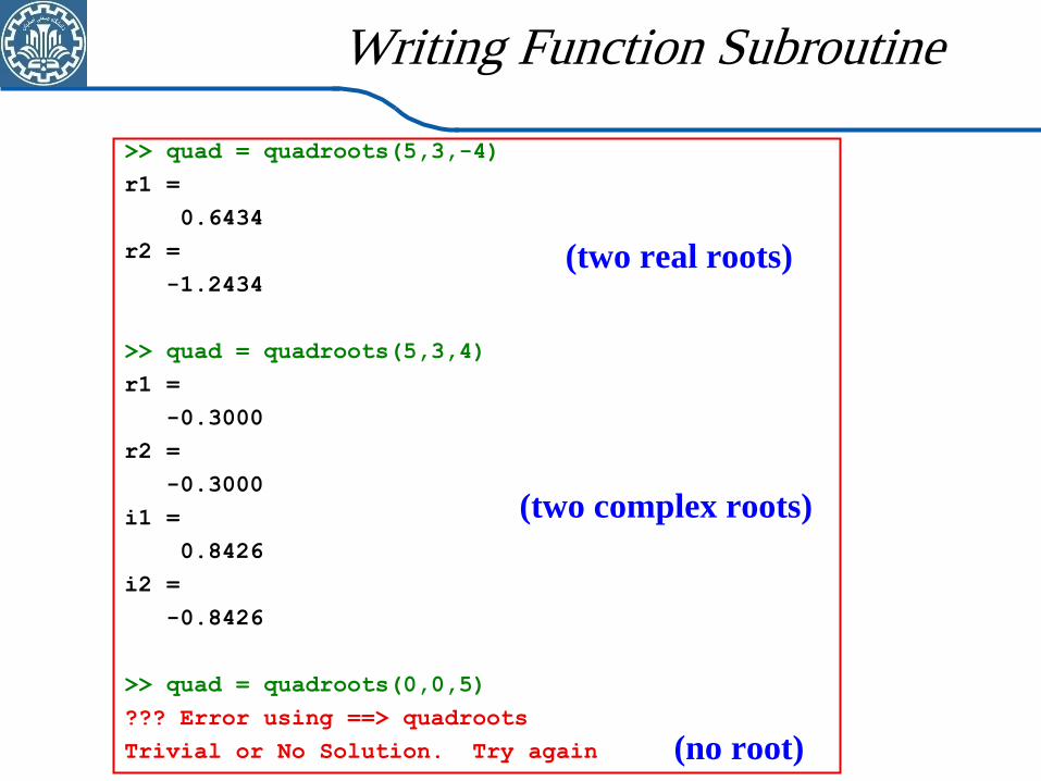
>> quad = quadroots(5,3,-4)
r1 =
0.6434
r2 =
-1.2434
>> quad = quadroots(5,3,4)
r1 =
-0.3000
r2 =
-0.3000
i1 =
0.8426
i2 =
-0.8426
>> quad = quadroots(0,0,5)
??? Error using ==> quadroots
Trivial or No Solution. Try again
(two real roots)
(two complex roots)
(no root)
Writing Function Subroutine