DATA 8Fall 2016

Slides created by Ani Adhikari and John DeNero

Review II, December 7 Inference; Theory of Prob/Stat

Plan for This Week● Today:

○ Complete Inference review○ Theory of Prob/Stat

● GSIs: today and tomorrow during lab times:○ First hour: review problems on particular topic○ Second hour: office hour○ Topics on Review links on data8.org

● Fri: Go see a dumb movie or relax in some other way

Final Exam● Monday December 12, 8:00 - 11:00● RSF Field House● Bring something to write with and something to erase

with; but not your breakfast. Water is OK.● We will provide a couple of reference sheets, with drafts

posted on Piazza during RRR week● 16 questions (six 5-pointers, five 6-pointers, five

8-pointers). ● Covers the whole course

Big Picture of Course Contents1. Python

2. Describing data

3. General concepts of inference

4. Theory of probability and statistics

5. Methods of inference

5. … Continued from Last Time

Inference: Tests of Hypotheses

Comparing Two Categorical Samples● Null: The two samples come from the same underlying

distribution in the population ● Test statistic: TVD between the distributions of the two

samples● Method:

○ Permutation: Under the null, pool the two samples, shuffle, and split into new samples A and B

● 16.1 (mitoses rating CKD/non-CKD; clump thickness rating cancerous/non-cancerous)

Comparing Two Numerical Samples● Null: The two samples come from the same underlying

distribution in the population.● Test statistic: difference between sample means (take

absolute value depending on alternative)● Methods (two!) for A/B Testing:

○ Permutation under the null: 10.4 (Deflategate), 16.2 (birth weight etc for smokers/nonsmokers), 16.3 (BTA RCT)

○ Bootstrap CI for difference: 16.2, 16.3

Causality● Tests of hypotheses can help decide that a difference is

not due to chance

● But they don’t say why there is a difference …

● Unless the data are from an RCT 16.3○ In that case a difference that’s not due to chance

can be ascribed to the treatment

Classification● Binary classification based on attributes 15.1

○ k-nearest neighbor classifiers● Training and test sets 15.2

○ Why these are needed○ How to generate them

● Implementation: 15.4○ Distance between two points○ Class of the majority of the k nearest neighbors

● Accuracy: Proportion of test set correctly classified 15.5

4. Probability and Statistics: Theory ● Descriptive statistics:

○ One variable○ Two variables

● Probability theory:○ Exact calculations○ Normal approximation for mean of large random

sample○ Accuracy and sample size

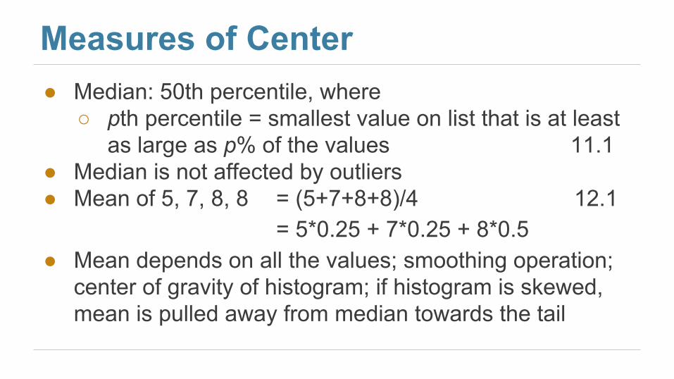
Measures of Center● Median: 50th percentile, where

○ pth percentile = smallest value on list that is at least as large as p% of the values 11.1

● Median is not affected by outliers● Mean of 5, 7, 8, 8 = (5+7+8+8)/4 12.1

= 5*0.25 + 7*0.25 + 8*0.5● Mean depends on all the values; smoothing operation;

center of gravity of histogram; if histogram is skewed, mean is pulled away from median towards the tail

Measure of Spread

root5

mean4

square of3

deviations from2

average1

Standard deviation (SD) =

Measures roughly how far off the values are from average

● 12.2

Chebychev’s BoundsRange Proportion

average ± 2 SDs at least 1 - 1/4 (75%)

average ± 3 SDs at least 1 - 1/9 (88.888…%)

average ± 4 SDs at least 1 - 1/16 (93.75%)

average ± z SDs at least 1 - 1/z²

no matter what the distribution looks like 12.2

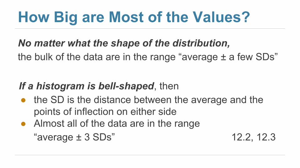
How Big are Most of the Values?No matter what the shape of the distribution,the bulk of the data are in the range “average ± a few SDs”

If a histogram is bell-shaped, then● the SD is the distance between the average and the

points of inflection on either side● Almost all of the data are in the range

“average ± 3 SDs” 12.2, 12.3

Bounds and normal approximations

12.3

Standard Units z“average ± z SDs” 12.2● z measures “how many SDs above average”● Almost all standard units are in the range (-5, 5)● To convert a value to standard units:

value - averagez = --------------------- SD

Definition of r

average of

product of x in standard

units

and y in standard

units

Correlation Coefficient (r) =

Measures how clustered the scatter is around a straight line 13.1

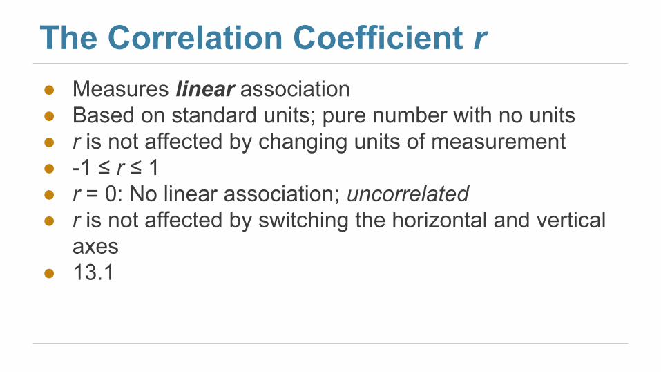
The Correlation Coefficient r● Measures linear association● Based on standard units; pure number with no units● r is not affected by changing units of measurement● -1 ≤ r ≤ 1● r = 0: No linear association; uncorrelated● r is not affected by switching the horizontal and vertical

axes● 13.1

Regression to the Mean

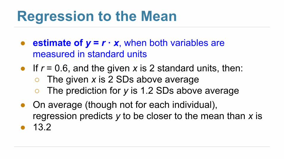
● estimate of y = r · x, when both variables are measured in standard units

● If r = 0.6, and the given x is 2 standard units, then:○ The given x is 2 SDs above average○ The prediction for y is 1.2 SDs above average

● On average (though not for each individual), regression predicts y to be closer to the mean than x is

● 13.2

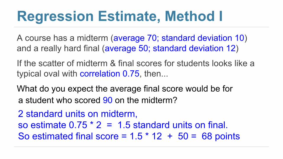
A course has a midterm (average 70; standard deviation 10)and a really hard final (average 50; standard deviation 12)

If the scatter of midterm & final scores for students looks like a typical oval with correlation 0.75, then...

What do you expect the average final score would be for

Regression Estimate, Method I

a student who scored 90 on the midterm?2 standard units on midterm,so estimate 0.75 * 2 = 1.5 standard units on final. So estimated final score = 1.5 * 12 + 50 = 68 points

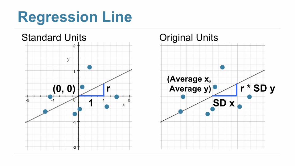
Regression LineStandard Units

(0, 0)1

r

Original Units

(Average x, Average y)

SD xr * SD y

Slope and Intercept

estimate of y = slope * x + intercept

● 13.2

Regression Estimate, Method IIThe equation of a regression line for estimating child’s height based on midparent height is

estimated child’s height = 0.64·midparent height + 22.64

Estimate the height of someone whose midparent height is 69 inches.

0.64*69 + 22.64 = 66.8 inches

Residuals● Error in regression estimate● One residual corresponding to each point (x, y)● residual = observed y - regression estimate of y

= vertical difference between point and line ● No matter what the shape of the scatter plot:

○ Residual plot does not show a trend○ Average of residuals = 0

13.6

Equally Likely Outcomes● If all outcomes are assumed equally likely, then

probabilities are proportions of outcomes:

number of outcomes that make A happenP(A) = --------------------------------------------------------------- total number of outcomes = proportion of outcomes that make A happen● 8.4

Probability: Exact Calculations ● Probabilities are between 0 (impossible) and 1 (certain)

● P(event happens) = 1 - P(the event doesn’t happen)

● Chance that two events A and B both happen= P(A happens) x P(B happens given that A has happened)

● If event A can happen in exactly one of two ways, thenP(A) = P(first way) + P(second way)

● 8.4

Updating Probabilities● Start with prior probabilities of two classes; priors can

be subjective● Known: likelihood of data, given each of the classes

● Acquire data according to these likelihoods

● Update the prior probabilities by finding posterior probabilities of the two classes, given the data

● Tree diagrams and Bayes’ Rule: 17.1, 17.2

Approximation: CLT Central Limit Theorem

If the sample is● large, and● drawn at random with replacement,

Then, regardless of the distribution of the population,

the probability distribution of the sample sum (or of the sample mean) is roughly bell-shaped 12.4

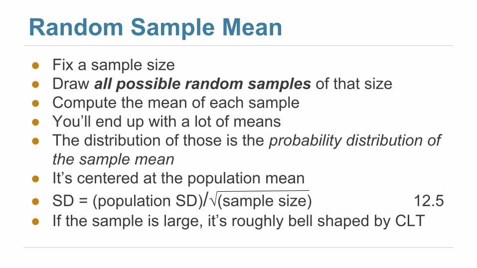
Random Sample Mean● Fix a sample size● Draw all possible random samples of that size● Compute the mean of each sample● You’ll end up with a lot of means● The distribution of those is the probability distribution of

the sample mean● It’s centered at the population mean● SD = (population SD)/√(sample size) 12.5● If the sample is large, it’s roughly bell shaped by CLT

Accuracy of Random Sample Mean ● Greater if SD of sample mean is smaller● Doesn’t depend on population size● Increases as sample size increases, because SD of

sample mean decreases● For 3 times the accuracy, you have to multiply the

sample size by a factor of 3² = 9● Square Root Law: If you multiply sample size by a

factor, accuracy goes up by the square root of the factor● 12.5

Application to Proportions● Fact: SD of 0-1 population ≤ 0.5 12.6 ● Total width of 95% CI for population proportion:

= 4 SDs of the sample proportion= 4 x (SD of 0-1 population)/√(sample size)

≤ 4 x 0.5/√(sample size)= 2 / √(sample size)

● So if you know the desired width of the interval, you can solve for (an overestimate of) the sample size