Revenue Maximization in Incentivized Social Advertising

Cigdem Aslay Francesco Bonchi Laks V.S. Lakshmanan Wei LuISI Foundation ISI Foundation Univ. of British Columbia Rupert Labs

Turin, Italy Turin, Italy Vancouver, Canada Mountain View, CA 94043cigdem.aslay@isi.it francesco.bonchi@isi.it laks@cs.ubc.ca w.lu@alumni.ubc.ca

ABSTRACTIncentivized social advertising, an emerging marketing model, pro-vides monetization opportunities not only to the owners of the so-cial networking platforms but also to their influential users by of-fering a “cut” on the advertising revenue. We consider a social net-work (the host) that sells ad-engagements to advertisers by insert-ing their ads, in the form of promoted posts, into the feeds of care-fully selected “initial endorsers” or seed users: these users receivemonetary incentives in exchange for their endorsements. The en-dorsements help propagate the ads to the feeds of their followers.Whenever any user engages with an ad, the host is paid some fixedamount by the advertiser, and the ad further propagates to the feedof her followers, potentially recursively. In this context, the prob-lem for the host is is to allocate ads to influential users, taking intoaccount the propensity of ads for viral propagation, and carefullyapportioning the monetary budget of each of the advertisers be-tween incentives to influential users and ad-engagement costs, withthe rational goal of maximizing its own revenue.

We show that, taking all important factors into account, the prob-lem of revenue maximization in incentivized social advertising cor-responds to the problem of monotone submodular function maxi-mization, subject to a partition matroid constraint on the ads-to-seeds allocation, and submodular knapsack constraints on the ad-vertisers’ budgets. We show that this problem is NP-hard and de-vise two greedy algorithms with provable approximation guaran-tees, which differ in their sensitivity to seed user incentive costs.

Our approximation algorithms require repeatedly estimating theexpected marginal gain in revenue as well as in advertiser payment.By exploiting a connection to the recent advances made in scal-able estimation of expected influence spread, we devise efficientand scalable versions of our two greedy algorithms. An extensiveexperimental assessment confirms the high quality of our proposal.

1. INTRODUCTIONThe rise of online advertising platforms has generated new op-

portunities for advertisers in terms of personalizing and targetingtheir marketing messages. Social networking platforms particularlycan gather large amounts of users’ shared posts that stretches be-yond general demographic and geographic data. This offers more

This work is licensed under the Creative Commons Attribution-NonCommercial-NoDerivatives 4.0 International License. To view a copyof this license, visit http://creativecommons.org/licenses/by-nc-nd/4.0/. Forany use beyond those covered by this license, obtain permission by emailinginfo@vldb.org.Proceedings of the VLDB Endowment, Vol. 10, No. 11Copyright 2017 VLDB Endowment 2150-8097/17/07.

advanced interest, behavioral, and connection-based targeting op-tions, enabling a level of personalization that is not achievable byother online advertising channels. Hence, advertising on social net-working platforms has been one of the fastest growing sectors inthe online advertising landscape: a market that did not exist un-til Facebook launched its first advertising service in May 2005, isprojected to generate $11 billion revenue by 2017, almost doublingthe 2013 revenue1.

Social advertising. Social advertising models are typically em-ployed by platforms such as Twitter, Tumblr, and Facebook throughthe implementation of promoted posts that are shown in the “newsfeed” of their users.2 A promoted post can be a video, an image, orsimply a textual post containing an advertising message. Social ad-vertising models of this type are usually associated with a cost perengagement (CPE) pricing scheme: the advertiser does not pay forthe ad impressions, but pays the platform owner (hereafter referredto as the host) only when a user actively engages with the ad. Theengagement can be in the form of a social action such as “like”,“share”, or “comment”: in this paper we blur the distinction be-tween these different types of actions, and generically refer to themall as engagements or clicks interchangeably.

Similar to organic (i.e., non-promoted) posts, promoted posts canpropagate from user to user in the network3, potentially triggering aviral contagion: whenever a user u engages with an ad i, the host ispaid some fixed amount by the advertiser (the CPE). Furthermore,u’s engagement with i appears in the feed of u’s followers, who arethen exposed to ad i and could in turn be influenced to engage withi, producing further revenue for the host [5, 35].

Incentivized social advertising. In this paper, we study the novelmodel of incentivized social advertising. Under this model, usersselected by the host as seeds for the campaign on a specific ad i,can take a “cut” on the social advertising revenue.

A recent report4 indicates that Facebook is experimenting withthe idea of incentivizing users. YouTube launched a revenue-sharing program for prominent users in 2007. Twitch, the streamingplatform of choice for gamers, lets partners make money throughrevenue sharing, subscriptions, and merchandise sales. YouNow, astreaming platform popular among younger users, earns money bytaking a cut of the tips and digital gifts that fans give its stars.

1http://www.unified.com/historyofsocialadvertising/

2According to a recent report, Facebook’s news feed ads have 21 times higherclick-through rate than standard web retargeting ads and 49 times the click-throughrate of Facebook’s right-hand side display ads: see https://blog.adroll.com/trends/facebook-exchange-news-feed-numbers.3Tumblr’s CEO D. Karp reported (CES 2014) that a normal post is reposted on aver-age 14 times, while promoted posts are on average reposted more than 10 000 times:http://yhoo.it/1vFfIAc.4http://www.theverge.com/2016/4/19/11455840/facebook-tip-

jar-partner-program-monetization

1238

In this work, we consider incentives that are determined by thetopical influence of the seed users for the specific ad. More con-cretely, given an ad i, the financial incentive that a seed user uwould get for engaging with i is a function of the social influencethat u has exhibited in the past in the topic of i. For instance, a userwho produces attention-capturing content about long-distance run-ning might be a good seed for endorsing a new model of runningshoes. In this case, her past demonstrated influence on this verytopic would be taken into consideration when defining the lump-sum amount for her engagement with the new model of runningshoes. The same user could be considered as a seed for a new modelof tennis shoes, but in that case the incentive might be lower, dueto her lower past influence demonstrated. To summarize, incentivesare paid by the host to users selected as seeds. These incentivescount as seeding costs and depend on the topic of the ad and theuser’s past demonstrated influence in the topic.

The incentive model above has several advantages. First, itcaptures in a uniform framework both the “celebrity-influencer”,whose incentives are naturally very high (like her social influence),and who are typically preferred by more traditional types of adver-tising such as TV ads; as well as the “ordinary-influencer” [6], anon-celebrity individual who is an expert in some specific topic,and thus has a relatively restricted audience, or tribe, that trust her.Second, incentives not only play their main role, i.e., encourage theseed users to endorse an advert campaign, but also, as a by-product,they incentivize users of the social media platform to become influ-ential in some topics by actively producing good-quality content.This has an obvious direct benefit for the social media platform.Revenue maximization. In the context of incentivized social ad-vertising, we study the fundamental problem of revenue maximiza-tion from the host perspective: an advertiser enters into an agree-ment with the host to pay, following the CPE model, a fixed pricecpe(i) for each engagement with ad i. The agreement also speci-fies the finite budget Bi of the advertiser for the campaign for adi. The host has to carefully select the seed users for the campaign:given the maximum amount Bi that it can receive from the ad-vertiser, the host must try to achieve as many engagements on thead i as possible, while spending as little as possible on the incen-tives for “seed” users. The host’s task gets even more challengingby having to simultaneously accommodate multiple campaigns bydifferent advertisers. Moreover, for a fixed time window (e.g., 1day, or 1 week), the host can select each user as the seed endorserfor at most one ad: this constraint maintains higher credibility forthe endorsements and avoids the undesirable situation where, e.g.,the same sport celebrity endorses Nike and Adidas in the same timewindow. Therefore two ads i and j, which are in the same topicalarea, naturally compete for the influential users in that area.

We show that, taking all important factors (such as topical rel-evance of ads, their propensity for social propagation, the topicalinfluence of users, seed incentives and advertiser budgets) into ac-count, the problem of revenue maximization in incentivized socialadvertising corresponds to the problem of monotone submodularfunction maximization subject to a partition matroid constraint onthe ads-to-seeds allocation, and submodular knapsack constraintson the advertisers’ budgets. This problem is NP-hard and further-more is far more challenging than the classical influence maximiza-tion problem (IM) [24] and its variants. For this problem, we de-velop two natural greedy algorithms, for which we provide formalapproximation guarantees. The two algorithms differ in their sensi-tivity to cost-effectiveness in the seed user selection:• Cost-Agnostic Greedy Algorithm (CA-GREEDY), which

greedily chooses the seeds based on the marginal gain in therevenue, without any information about the incentive costs;

• Cost-Sensitive Greedy Algorithm (CS-GREEDY), whichgreedily chooses the seed users based on the rate of marginalgain in revenue per marginal gain in the advertiser’s paymentfor each advertiser.

Our results generalize the results of Iyer et al. [22, 23] on sub-modular function maximization by (i) generalizing from a singlesubmodular knapsack constraint to multiple submodular knapsackconstraints, and (ii) by handling an additional partition matroidconstraint. Our theoretical analysis leverages the notion of curva-ture of submodular functions.

Our approximation algorithms require repeatedly estimating theexpected marginal gain in revenue as well in advertiser payment.We leverage recent advances in scalable estimation of expected in-fluence spread and devise scalable algorithms for revenue maxi-mization in our model.Contributions and roadmap.• We propose incentivized social advertising, and formulate a

fundamental problem of revenue maximization from the hostperspective (Section 2).• We prove the hardness of our problem and we devise two

greedy algorithms with approximation guarantees. The first(CA-GREEDY) is agnostic to users’ incentives during the seedselection while the other (CS-GREEDY) is not (Section 3).• We devise scalable versions of our approximation algorithms

(Section 4). Our comprehensive experimentation on real-world datasets (Section 5) confirms the scalability of ourmethods and shows that the scalable version of CS-GREEDYconsistently outperforms that of CA-GREEDY, and is far su-perior to natural baselines.

Some proofs are omitted here for brevity and can be found in [1].

2. PROBLEM STATEMENTBusiness model: the advertiser. An advertiser5 i enters into anagreement with the host, the owner of the social networking plat-form, for an incentivized social advertising campaign on its ad. Theadvertiser agrees to pay the host:

1. an incentive ci(u) for each seed user u chosen to endorse ad i;we let Si denote the set of users selected to endorse ad i;

2. a cost-per-engagement amount cpe(i) for each user that engageswith (e.g., clicks) its ad i.

An advertiser i has a finite budget Bi that limits the amount it canspend on the campaign for its ad.Business model: the host. The host receives from advertiser i:

1. a description of the ad i (e.g., a set of keywords) which allows thehost to map the ad to a distribution ~γi over a latent topic space;

2. a commercial agreement that specifies the cost-per-engagementamount cpe(i) and the campaign budget Bi.The host is in charge of running the campaign, by selecting

which users and how many to allocate as a seed set Si for eachad i, and by determining their incentives. Given that these deci-sions must be taken before the campaign is started, the host hasto reason in terms of expectations based on past performance. Letσi(Si) denote the expected number of clicks ad i receives when us-ing Si as the seed set of incentivized users. The host models thetotal payment that advertiser i needs to make for its campaign,denoted ρi(Si), as the sum of its total costs for the expected ad-engagements (e.g., clicks), and for incentivizing its seed users:5We assume each advertiser has one ad to promote per time window, and use i to referto the i-th advertiser and its ad interchangeably.

1239

i.e., ρi(Si) = πi(Si) + ci(Si) where πi(Si) = cpe(i) · σi(Si)and ci(Si) :=

∑u∈Si ci(u), where ci(u) denotes the incentive

paid to a candidate seed user u for ad i. We assume ci(u) is amonotone function f of the influence potential of u, capturing theintuition that seeds with higher expected spread cost more: i.e.,ci(u) := f(σi({u})).

Notice that the expected revenue of the host from the engage-ments to ad i is just πi(Si), as the cost ci(Si) paid by the advertiserto the host for the incentivizing influential users, is in turn paid bythe host to the seeds. In this setting, the host faces the followingtrade-off in trying to maximize its revenue. Intuitively, targeting in-fluential seeds would increase the expected number of clicks, whichin turn could yield a higher revenue. However, influential seeds costmore to incentivize. Since the advertiser has a fixed overall budgetfor its campaign, the higher seeding cost may come at the expenseof reduced revenue for the host. Finally, an added challenge is thatthe host has to serve many advertisers at the same time, with po-tentially competitive ads, i.e., ads which are very close in the topicspace.Data model, topic model, and propagation model. The host,owns: a directed graph G = (V,E) representing the social net-work, where an arc (u, v) means that user v follows user u, andthus v can see u’s posts and may be influenced by u. The host alsoowns a topic model for ads and users’ interests, defined by a hiddenvariable Z that can range over L latent topics. A topic distributionthus abstracts the interest pattern of a user and the relevance of anad to those interests. More precisely, the topic model maps each adi to a distribution ~γi over the latent topic space:

γzi = Pr(Z = z|i), with∑L

z=1γzi = 1.

Finally, the host uses a topic-aware influence propagation modeldefined on the social graph G and the topic model. The propaga-tion model governs the way in which ad impressions propagate inthe social network, driven by topic-specific influence. In this work,we adopt the Topic-aware Independent Cascade model6 (TIC) pro-posed by Barbieri et al. [8] which extends the standard Indepen-dent Cascade (IC) model [24]: In TIC, an ad is represented by atopic distribution, and the influence strength from user u to v isalso topic-dependent, i.e., there is a probability pzu,v for each topicz. In this model, when a node u clicks an ad i, it gets one chance ofinfluencing each of its out-neighbors v that has not clicked i. Thisevent succeeds with a probability equal to the weighted average ofthe arc probabilities w.r.t. the topic distribution of ad i:

piu,v =∑L

z=1γzi · pzu,v. (1)

Using this stochastic propagation model the host can determine theexpected spread σi(Si) of a given campaign for ad i when usingSi as seed set. For instance, the influence value of a user u forad i is defined as the expected spread of the singleton seed {u}for the given the description for ad i, under the TIC model, i.e.,σi({u}): this is the quantity that is used to determine the incentivefor a candidate seed user u to endorse the ad i.The revenue maximization problem. Hereafter we assume a fixedtime window (say a 24-hour period) in which the revenue maxi-mization problem is defined. Within this time window we have hadvertisers with ad description ~γi, cost-per-engagement cpe(i), andbudgetBi, i ∈ [h]. We define an allocation ~S as a vector of h pair-wise disjoint sets (S1, · · · , Sh) ∈ 2V × · · · × 2V , where Si is the6Note that the use of the topic-based model is orthogonal to the technical developmentand contributions of our work. Specifically, if we assume that the topic distributions ofall ads and users are identical, the TIC model reduces to the standard IC model. Thetechniques and results in the paper remain intact.

seed set assigned to advertiser i to start the ad-engagement propa-gation process. Within the time window, each user in the platformcan be selected to be seed for at most one ad, that is, Si ∩ Sj = ∅,i, j ∈ [h]. We denote the total revenue of the host from advertisersas the sum of the ad-specific revenues:

π(~S) =∑

i∈[h]πi(Si).

Next, we formally define the revenue maximization problem forincentivized social advertising from the host perspective. Note thatgiven an instance of the TIC model on a social graphG, for each adi, the ad-specific influence probabilities are determined by Eq. (1).

Problem 1 (REVENUE-MAXIMIZATION (RM)). Given a socialgraphG = (V,E), h advertisers, cost-per-engagement cpe(i) andbudget Bi, i ∈ [h], ad-specific influence probabilities piu,v andseed user incentive costs ci(u), u, v ∈ V , i ∈ [h], find a feasibleallocation ~S that maximizes the host’s revenue:

maximize~S

π(~S)

subject to ρi(Si) ≤ Bi,∀i ∈ [h],

Si ∩ Sj = ∅, i 6= j, ∀i, j ∈ [h].

In order to avoid degenerate problem instances, we assume thatno single user incentive exceeds any advertiser’s budget. This en-sures that every advertiser can afford at least one seed node.

3. HARDNESS AND APPROXIMATIONHardness. We first show that Problem 1 (RM) is NP-hard. We

recall that a set function f : 2U → R≥0 is monotone if for S ⊂T ⊆ U , f(S) ≤ f(T ). We define the marginal gain of an elementxw.r.t. S ⊂ U as f(x|S) := f(S∪{x})−f(S). A set function f issubmodular if for S ⊂ T ⊂ U and x ∈ U \ T , f(x|T ) ≤ f(x|S),i.e., the marginal gains diminish with larger sets.

It is well known that the influence spread function σi(·) ismonotone and submodular [24], from which it follows that the ad-specific revenue function πi(·) is monotone and submodular. Fi-nally, since the total revenue function, π(~S) =

∑i∈[h] πi(Si), is

a non-negative linear combination of monotone and submodularfunctions, these properties carry over to π(~S). Likewise, for eachad i, the payment function ρi(·) is a non-negative linear combina-tion of two monotone and submodular functions, πi(·) and ci(·),and so is also monotone and submodular. Thus, the constraintsρi(Si) ≤ Bi, i ∈ [h], in Problem 1 are submodular knapsackconstraints. We start with our hardness result.

Theorem 1. Problem 1 (RM) is NP-hard.

Proof. Consider the special case with one advertiser, i.e., h = 1.Then we have one submodular knapsack constraint and no partitionmatroid constraint. This corresponds to maximizing a submodularfunction subject to a submodular knapsack constraint, the so-calledSubmodular Cost Submodular Knapsack (SCSK) problem, whichis known to be NP-hard [23]. Since this is a special case of Problem1, the claim follows.

Next, we characterize the constraint that the allocation ~S =(S1, · · · , Sh) should be composed of pairwise disjoint sets, i.e.,Si ∩ Sj = ∅, i 6= j, ∀i, j ∈ [h]. We will make use of the followingnotions on matroids.

Definition 1 (Independence System). A set system (E , I) definedwith a finite ground set E of elements, and a family I of subsetsof E is an independence system if I is non-empty and if it satisfiesdownward closure axiom, i.e., X ∈ I ∧ Y ⊆ X → Y ∈ I.

1240

Definition 2 (Matroid). An independence system (E , I) is a ma-troid M = (E , I) if it also satisfies the augmentation axiom: i.e.,X ∈ I ∧ Y ∈ I ∧ |Y | > |X| → ∃e ∈ Y \X : X ∪ {e} ∈ I.

Definition 3 (Partition Matroid). Let E1, · · · , El be a partition ofthe ground set E into l non-empty disjoint subsets. Let di be aninteger, 0 ≤ di ≤ |Ei|. In a partition matroid M = (E , I), a set Xis defined to be independent iff, for every i, 1 ≤ i ≤ l, |X ∩ Ei| ≤di. That is, I = {X ⊆ E : |X ∩ Ei| ≤ di, ∀i = 1, · · · , l}.

Lemma 1. The constraint that in an allocation ~S = (S1, · · · , Sh),the seed sets Si are pairwise disjoint is a partition matroid con-straint over the ground set E of all (node, advertiser) pairs.

Therefore, the RM problem corresponds to the problem of sub-modular function maximization subject to a partition matroid con-straint M = (E , I), and h submodular knapsack constraints.Approximation analysis. Next lemma states that the constraints ofthe RM problem together form an independence system defined onthe ground set E . This property will be leveraged later in developingapproximation algorithms. Given the partition matroid constraintM = (E , I), and h submodular knapsack constraints, let C denotethe family of subsets, defined on E , that are feasible solutions to theRM problem.

Lemma 2. The system (E , C) is an independence system.

Our theoretical guarantees for our approximation algorithms tothe RM problem depend on the notion of curvature of submodularfunctions. Recall that f(j|S), j 6∈ S, denotes the marginal gainf(S ∪ {j})− f(S).

Definition 4 (Curvature). [15] Given a submodular function f ,the total curvature κf of f is defined as

κf = 1−minj∈Vf(j|V \ {j})f({j}) ,

and the curvature κf (S) of f wrt a set S is defined as

κf (S) = 1−minj∈Sf(j|S \ {j})f({j}) .

It is easy to see that 0 ≤ κf = κf (V ) ≤ 1. Intuitively, the cur-vature of a function measures the deviation of f from modularity:modular functions have a curvature of 0, and the further away f isfrom modularity, the larger κf is. Similarly, the curvature κf (S) off wrt a set S reflects how much the marginal gains f(j | S) candecrease as a function of S, measuring the deviation from modu-larity, given the context S. In the next subsections, we propose twogreedy approximation algorithms for the RM problem. The firstof these, Cost-Agnostic Greedy Algorithm (CA-GREEDY), greed-ily chooses the seed users solely based on the marginal gain in therevenue, without considering seed user incentive costs. The second,Cost-Sensitive Greedy Algorithm (CS-GREEDY), greedily choosesthe seed users based on the rate of marginal gain in revenue permarginal gain in the advertiser’s payment for each advertiser.

We note that Iyer et al. [22, 23] study a restricted special caseof the RM problem, referred as Submodular-Cost Submodular-Knapsack (SCSK), and propose similar cost-agnostic and cost-sensitive algorithms. Our results extend theirs in two major ways.First, we extend from a single advertiser to multiple advertisers(i.e., from a single submodular knapsack constraint to multiplesubmodular knapsack constraints). Second, unlike SCSK, our RMproblem is subject to an additional partition matroid constraint onthe ads-to-seeds allocation, which naturally arises when multipleadvertisers are present.

3.1 Cost-Agnostic Greedy AlgorithmThe Cost-Agnostic Greedy Algorithm (CA-GREEDY) for the

RM problem, whose pseudocode is provided in Algorithm 1,chooses at each iteration a (node, advertiser) pair that provides themaximum increase in the revenue of the host. Let Xg ⊆ E de-note the greedy solution set of (node,advertiser) pairs, returned byCA-GREEDY, having one-to-one correspondence with the greedyallocation ~Sg , i.e., Si = {u : (u, i) ∈ Xg}, ∀Si ∈ ~Sg . Let X tgdenote the greedy solution after t iterations of CA-GREEDY. Ateach iteration t, CA-GREEDY first finds the (node,advertiser) pair(u∗, i∗) that maximizes πi(u | St−1

i ), and tests whether addingthis pair to the current greedy solutionX t−1

g would violate any con-straint: if X t−1

g ∪ {(u∗, i∗)} is feasible, the pair (u∗, i∗) is addedto the greedy solution as the t-th (node,advertiser) pair. Otherwise,(u∗, i∗) is removed from the current ground set of (node,advertiser)pairs Et−1. CA-GREEDY terminates when there is no feasible(node,advertiser) pair left in the current ground set Et−1.

Observation 1. Being monotone and submodular, the total revenuefunction π( ~Sg) has a total curvature κπ , given by:

κπ = 1−min(u,i)∈Eπi(u | V \ {u})

πi({u}).

We will make use of the following notions in our results on ap-proximation guarantees.

Definition 5 (Upper and lower rank). Let (E , C) be an indepen-dence system. Its upper rank R and lower rank r are defined as thecardinalities of the smallest and largest maximal independent sets:

r = min{|X| : X ∈ C and X ∪ {(u, i)} 6∈ C, ∀(u, i) 6∈ X},

R = max{|X| : X ∈ C and X ∪ {(u, i)} 6∈ C, ∀(u, i) 6∈ X}.

When the independence system is a matroid, r = R, as all max-imal independent sets have the same cardinality.

Theorem 2. CA-GREEDY achieves an approximation guarantee

of1

κπ

[1−

(R− κπR

)r]to the optimum, where κπ is the total

curvature of the total revenue function π(·), r and R are respec-tively the lower and upper rank of (E , C). This bound is tight.

Proof. We note that the family C of subsets that constitute feasi-ble solutions to the RM problem form an independence systemdefined on E (Lemma 2). Given this, the approximation guaran-tee of CA-GREEDY directly follows from the result of Conforti etal. [15, Theorem 5.4] for submodular function maximization sub-ject to an independence system constraint. However, the tightnessdoes not directly follow from the tightness result in [15], which weaddress next.

We now exhibit an instance to show that the bound is tight. Con-sider one advertiser, i.e., h = 1. The network is shown in Fig-ure 1, where all influence probabilities are 1. The incentive costsfor nodes are as shown in the figure, while cpe(.) = 1. The budgetis B = 7. It is easy to see that the lower rank is r = 1, correspond-ing to the maximal feasible seed set S = {b}, while the upperrank is R = 2, e.g., corresponding to maximal feasible seed setssuch as T = {a, c}. Furthermore, the total curvature is κπ = 1.On this instance, the optimal solution is T which achieves a rev-enue of 6. In its first iteration, CA-GREEDY could choose b asa seed. Once it does, it is forced to the solution S = {b} as nomore seeds can be added to S. The revenue of CA-GREEDY is

3 =1

κπ

[1−

(R− κπR

)r]OPT = 1

2· 6.

1241

Figure 1: Instance illustrating tightness of bound in Theorem 2.Discussion. We next discuss the significance and the meaning ofthe bound in Theorem 2. Notice that when there is just one adver-tiser, TIC reduces to IC. Even for this simple setting, the bound onCA-GREEDY is tight. By a simple rearrangement of the terms, wehave:

1

κπ

[1−

(R− κπR

)r]≥ 1

κπ

(1− e

−κπ·r

R

).

Clearly, the cost-agnostic approximation bound improves asr

Rap-

proaches 1, achieving the best possible value when r = R. Asa special case, the cost-agnostic approximation further improveswhen the independence system (E , C) is a matroid since for a ma-troid r = R always holds: e.g., consider the standard IM prob-lem [24] which corresponds to submodular function maximizationsubject to a uniform matroid. Here, π(·) = σ(·). Then the approxi-

mation guarantee becomes1

κπ

(1− e−κπ

), providing a slight im-

provement over the usual (1 − 1/e)-approximation, thanks to thecurvature term κπ .7 This remark is also valid for budgeted influ-ence maximization [26] with uniform seed costs. For more generalinstances of the problem, the guarantee depends on the characteris-tics of the instance, specifically, the lower and upper ranks and thecurvature. This kind of instance dependent bound is characteristicof submodular function maximization over an independence sys-tem [15,25]. Specifically for the RM problem, given its constraints,the values of r and R are dictated by the values of h payment func-tions over all feasible allocations. For instance, given our assump-tion that every advertiser can afford at least one seed, we alwayshave r ≥ h. The worst-case value r = h corresponds to the casein which each advertiser i is allocated a single seed node ui whosepayment ρi(ui) exhausts its budget Bi. Similarly for R, withoutusing any particular assumption on Bi, ∀i ∈ [h], we always haveR ≤ min(n,

∑i∈[h] bBi/cpe(i)c). Notice also that:

1

κπ

[1−

(R− κπR

)r]=

1

κπ

[1−

(1− κπ

R

)r](2)

≥ 1

κπ

[1−

(1− κπ

R

)]=

1

κπ

κπR

=1

R(3)

Hence, the worst-case approximation is always bounded by 1/R.

3.2 Cost-Sensitive Greedy AlgorithmThe Cost-sensitive greedy algorithm (CS-GREEDY) for the RM

problem is similar to CA-GREEDY. The main difference is that ateach iteration t, CS-GREEDY first finds the (node,advertiser) pair

(u∗, i∗) that maximizesπi(u | St−1

i )

ρi(u | St−1i )

, and tests whether the ad-

dition of this pair to the current greedy solution set X t−1g would

violate any matroid or knapsack independence constraint: if the ad-dition is feasible, the pair (u∗, i∗) is added to the greedy solution7Note that κπ ≤ 1 always. Hence, the extent of improvement increases asthe total curvature κπ decreases.

Algorithm 1: CA-GREEDY

Input : G = (V,E), Bi, cpe(i), ~γi, ∀i ∈ [h],ci(u),∀i ∈ [h], ∀u ∈ V

Output: ~Sg = (S1, · · · , Sh)1 t← 1, E0 ← E , X 0

g ← ∅2 S0

i ← ∅, ∀i ∈ [h]

3 while Et−1 6= ∅ do4 (u∗, i∗)← argmax (u,i)∈Et−1 πi(u | St−1

i )

5 if (X t−1g ∪ {(u∗, i∗)}) ∈ C then

6 Sti∗ ← St−1i∗ ∪ {u∗}

7 Stj ← St−1j , ∀j 6= i∗

8 X tg ← X t−1g ∪ {(u∗, i∗)}

9 Et ← Et−1 \ {(u∗, i∗)}10 t← t+ 1

11 else12 Et−1 ← Et−1 \ {(u∗, i∗)}13 Si ← St−1

i , ∀i ∈ [h]

14 return ~Sg = (S1, · · · , Sh)

as the t-th (node,advertiser) pair. Otherwise, (u∗, i∗) is removedfrom the current ground set Et−1. CS-GREEDY terminates whenthere is no (node,advertiser) pair left in the current ground set Et−1.CS-GREEDY can be obtained by simply replacing Line 4 of Algo-rithm 1 with

(u∗, i∗)← argmax(u,i)∈Et−1

πi(u | St−1i )

ρi(u | St−1i )

.

Theorem 3. CS-GREEDY achieves an approximation guaranteeof

1− R · ρmaxR · ρmax + (1− max

i∈[h]κρi) · ρmin

to the optimum where R is the upper rank of (E , C), κρi is the totalcurvature of ρi(·), ∀i ∈ [h], ρmax := max

(u,i)∈Eρi(u) and ρmin :=

min(u,i)∈E

ρi(u) are respectively the maximum and minimum singleton

payments over all (node, advertiser) pairs.

Proof. We use ~S∗ = (S∗1 , ..., S∗h) and ~Sg = (S1, ..., Sh) to denote

the optimal and greedy allocations respectively, and X ∗ and X gto denote the corresponding solution sets. Specifically, S∗i = {u :(u, i) ∈ X ∗}, and Si = {u : (u, i) ∈ Xg}. We denote by X tg theresult of the greedy solution after t iterations. LetK = |Xg| denotethe size of the greedy solution. Thus,X g = XKg . By submodularityand monotonicity:

π( ~S∗) ≤ π( ~Sg)+∑

(u,i)∈X∗\Xg

πi(u | Si) ≤ π( ~Sg)+∑

(u,i)∈X∗πi(u | Si).

At each iteration t, the greedy algorithm first finds the (node,

advertiser) pair (u∗, i∗) ← argmax(u,i)∈Et−1

πi(u | St−1i )

ρi(u | St−1i )

, and tests

whether the addition of this pair to the current greedy solution setX t−1g would violate any independence constraint. If (u∗, i∗) is fea-

sible, i.e., if X t−1g ∪{(u∗, i∗)} ∈ C, then the pair (u∗, i∗) is added

to the greedy solution as the t-th (node, advertiser) pair; otherwise,(u∗, i∗) is removed from the current ground set Et−1. In what fol-lows, for clarity, we use the notation (ut, it) to denote the (node,advertiser) pair that is successfully added by the greedy algorithmto X t−1

g in iteration t.Let U t denote the set of (node, advertiser) pairs that the greedy

algorithm tested for possible addition to the greedy solution in

1242

the first (t + 1) iterations before the addition of the (t + 1)-stpair (ut+1, it+1) into X tg . Thus, U t \ U t−1 includes the t-th pair(ut, it) that was successfully added to X t−1

g , as well as all thepairs that were tested for addition into X tg but failed the indepen-

dence test. Thus, ∀(u, i) ∈ U t \ U t−1, we haveπi(u | Sti )ρi(u | Sti )

≥

πit+1(ut+1 | Stit+1)

ρit+1(ut+1 | Stit+1)

, since they were tested for addition to X tg be-

fore (ut+1, it+1), but failed the independence test. For all (u, i) ∈

U t \ U t−1, we haveπi(u | St−1

i )

ρi(u | St−1i )

≤πit(ut | St−1

it)

ρit(ut | St−1it

). since they

were not good enough to be added to X t−1g as the t-th pair. Note

that, the greedy algorithm terminates when there is no feasiblepair left in the ground set. Hence after K iterations, EK containsonly the infeasible pairs that violate some matroid or knapsackconstraint. Thus, we have X ∗ =

⋃Kt=1[X

∗ ∩ (U t \ U t−1)]. LetU∗t := X ∗ ∩ (U t \ U t−1). Notice that X ∗ =

⋃Kt=1 U

∗t . Then, we

have:

π( ~S∗) ≤ π( ~Sg) +∑

(u,i)∈X∗

πi(u | Si)

= π( ~Sg) +

K∑t=1

∑(u,i)∈U∗

t

πi(u | Si)

≤ π( ~Sg) +K∑t=1

∑(u,i)∈U∗

t

πit(ut | St−1it

)

ρit(ut | St−1it

)· ρi(u | St−1

i ).

The last inequality is due to the fact that ∀(u, i) ∈ U∗t :

πi(u | Si) ≤ πi(u | St−1i ) ≤

πit(ut | St−1it

)

ρit(ut | St−1it

)· ρi(u | St−1

i ),

where the first inequality follows from submodularity and the sec-ond follows from the greedy choice of (node, advertiser) pairs.Continuing, we have:

π( ~S∗) ≤ π( ~Sg) +K∑t=1

πit(ut | St−1it

)

ρit(ut | St−1it

)

∑(u,i)∈U∗

t

ρi(u | St−1i )

≤ π( ~Sg) +K∑t=1

πit(ut | St−1it

)

ρit(ut | St−1it

)·K∑t=1

∑(u,i)∈U∗

t

ρi(u)

= π( ~Sg) +

K∑t=1

πit(ut | St−1it

)

ρit(ut | St−1it

)·∑

(u,i)∈X∗

ρi(u)

≤ π( ~Sg) + π( ~Sg) ·R · max

(u,i)∈X∗ρi(u)

mint∈[1,K]

ρit(ut | St−1it

)(4)

where the last inequality follows from the fact that π( ~Sg) =∑Kt=1 πit(ut | S

t−1it

) and |X ∗| ≤ R since X ∗ ∈ C. Let(utm , itm) := argmin

t∈[1,K]

ρit(ut | St−1it

) and let (umin, imin) :=

argmin(u,i)∈E

ρi(u | V \ {u}). Being monotone and submodular, each

ρi(·) has the total curvature κρi = 1−minu∈Vρi(u | V \ {u})

ρi(u).

Hence, for ρimin(·), we have:

1− κρimin ≤ρimin(umin | V \ {umin})

ρimin(umin), (5)

where the inequality above follows from the definition of totalcurvature. Then, using submodularity and Eq.5, we obtain:

mint∈[1,K]

ρit(ut | St−1it

) = ρitm (utm | Stm−1itm

)

≥ ρitm (utm | V \ {utm})≥ ρimin(umin | V \ {umin})≥ (1− κρimin ) · ρimin(umin)≥ (1−max

i∈[h]κρi) · min

(u,i)∈Eρi(u). (6)

Continuing from where we left in Eq.4 and using Eq.6, we have:

π( ~S∗) ≤ π( ~Sg) + π( ~Sg) ·R · max

(u,i)∈X∗ρi(u)

mint∈[1,K]

ρit(ut | St−1it

)

≤ π( ~Sg) ·

1 +

R · max(u,i)∈E

ρi(u)

(1−maxi∈[h]

κρi) · min(u,i)∈E

ρi(u)

= π( ~Sg) ·

1 +R · ρmax

(1−maxi∈[h]

κρi) · ρmin

(7)

Rearranging the terms we obtain:

π( ~Sg) ≥ π( ~S∗) ·(1−max

i∈[h]κρi) · ρmin

(1−maxi∈[h]

κρi) · ρmin +R · ρmax

= π( ~S∗) ·

1− R · ρmaxR · ρmax + (1−max

i∈[h]κρi) · ρmin

.

Discussion. We next discuss the significance and the meaning ofthe bounds. Notice that the value of the cost-sensitive approxima-tion bound improves as the ratio

ρmaxρmin

decreases, as Eq. 7 shows.

Since ρmax ≤ mini∈[h]

Bi, we can see that as the value of ρmax de-

creases, intuitively r would increase, for the corresponding maxi-mal independent set of minimum size could pack more seeds underthe knapsack constraints. Similarly, if the value of ρmin increases,R would decrease since the corresponding maximal independentset of maximum size could pack fewer seeds under the knapsackconstraints. Thus, intuitively as

ρmaxρmin

decreases,r

Rwould in-

crease. When this happens, both cost-agnostic and cost-sensitiveapproximations improve.

At one extreme, when κρi = 0, ∀i ∈ [h], i.e., when ρi(·)is modular ∀i ∈ [h], we have linear knapsack constraints. Thus,Theorem 2 and Theorem 3 respectively provide cost-agnostic andcost-sensitive approximation guarantees for the Budgeted InfluenceMaximization problem [26,31] for the case of multiple advertisers,with an additional matroid constraint. At the other extreme, whenmaxi∈[h]

κρi = 1, which is the case for totally normalized and saturated

functions (e.g., matroid rank functions), the approximation guaran-tee of CS-GREEDY is unbounded, i.e., it becomes degenerate. Thisis similar to the result of [22] for the SCSK problem whose cost-sensitive approximation guarantee becomes unbounded. Neverthe-less, combining the results of the cost-agnostic and cost-sensitivecases, we can obtain a bounded approximation. On the other hand,while CA-GREEDY always has a bounded worst-case guarantee,

1243

our experiments show that CS-GREEDY empirically obtains higherrevenue.8

4. SCALABLE ALGORITHMSWhile Algorithms CA-GREEDY and CS-GREEDY provide ap-

proximation guarantees, their efficient implementation is a chal-lenge, as both of them require a large number of influence spreadestimations: in each iteration t, for each advertiser i and each nodeu ∈ V \ St−1

i , the algorithms need to compute πi(u | St−1i ) and

πi(u | St−1i )/ρi(u | St−1

i ) respectively.Computing the exact influence spread σ(S) of a given seed set S

under the IC model is #P-hard [13], and this hardness carries overto the TIC model. In recent years, significant advances have beenmade in efficiently estimating σ(S). A natural question is whetherthey can be adapted to our setting, an issue we address next.

4.1 Scalable Influence Spread EstimationTang et al. [34] proposed a near-linear time randomized algo-

rithm for influence maximization, called Two-phase Influence Max-imization (TIM), building on the notion of “reverse-reachable”(RR) sets proposed by Borgs et al. [10]. Random RR-sets are crit-ical in the efficient estimation of influence spread. Tang et al. [33]subsequently proposed an algorithm called IMM that improvesupon TIM by tightening the lower bound on the number of ran-dom RR-sets required to estimate influence with high probability.The difference between TIM and IMM is that the lower bound usedby TIM ensures that the number of random RR-sets it uses is suf-ficient to estimate the spread of any seed set of a given size s. Bycontrast, IMM uses a lower bound that is tailored for the seed thatis greedily selected by the algorithm. Nguyen et al. [32], adaptingideas from TIM [34], and the sequential sampling design proposedby Dagum et al. [16], proposed an algorithm called SSA that pro-vides significant run-time improvement over TIM and IMM.

These algorithms are designed for the basic influence maximiza-tion problem and hence require knowing the number of seeds asinput. In our problem, the number of seeds is not fixed, but is dy-namic and depends on the budget and partition matroid constraints.Thus a direct application of these algorithms is not possible.

Aslay et al. [4] recently proposed a technique for efficient seedselection for IM when the number of seeds required is not predeter-mined but can change dynamically. However, their technique can-not handle the presence of seed user incentives which, in our set-ting, directly affects the number of seeds required to solve the RMproblem. In this section, we derive inspiration from their technique.First, though we note that for CA-GREEDY, in each iteration, foreach advertiser, we need to find a feasible node that yields the max-imum marginal gain in revenue, and hence the maximum marginalspread. By contrast, in CS-GREEDY, we need to find the node thatyields the maximum rate of marginal revenue per marginal gain inpayment, i.e., πi(u | St−1

i )/ρi(u | St−1i ).

To find such node uti we must compute σi(v|St−1i ), ∀v : (v, i) ∈

Et−1: notice that node uti might even correspond to the node thathas the minimum marginal gain in influence spread for iteration t.Thus, any scalable realization of CS-GREEDY should be capable ofworking as an influence spread oracle that can efficiently computeπi(u | St−1

i )/ρi(u | St−1i ) for all u ∈ {v : (v, i) ∈ Et−1}.

Among the state-of-the-art IM algorithms [32–34], onlyTIM [34] can be adapted to serve as an influence oracle. For agiven set size s, the derivation of the number of random RR-sets

8It remains open whether the approximation bound for CS-GREEDY istight. Interestingly, on the instance (Fig. 1) used in the proof of Theorem2,CS-GREEDY obtains the optimal solution T = {a, c}.

that TIM uses is done such that the influence spread of any set ofat most s nodes can be accurately estimated. On the other hand,even though IMM [33] and SSA [32] provide significant run-timeimprovements over TIM, they inherently cannot perform this es-timation task accurately: the sizes of the random RR-sets samplethat these algorithms use are tuned just for accurately estimatingthe influence spread of only the approximate greedy solutions; thesample sizes used are inadequate for estimating the spread of ar-bitrary seed sets of a given size. Thus, we choose to extend TIMto devise scalable realizations of CA-GREEDY and CS-GREEDY,namely, TI-CARM and TI-CSRM. Next, we describe how to ex-tend the ideas of RR-sets sampling and TIM’s sample size determi-nation technique to obtain scalable approximation algorithms forthe RM problem: TI-CARM and TI-CSRM.

4.2 Scalable Revenue MaximizationFor the scalable estimation of influence spread, in this sec-

tion we devise TI-CARM and TI-CSRM, scalable realizations ofCA-GREEDY and CS-GREEDY, based on the notion of Reverse-Reachable sets [10] and adapt the sample size determination pro-cedure employed by TIM [34] to achieve a certain estimation accu-racy with high confidence.

Reverse-Reachable (RR) sets [10]. Under the IC model, a ran-dom RR-setR fromG is generated as follows. First, for every edge(u, v) ∈ E, remove it from G w.p. 1 − pu,v: this generates a pos-sible world (deterministic graph) X . Second, pick a target node wuniformly at random from V . Then, R consists of the nodes thatcan reach w in X . For a sufficient sample R of random RR-sets,the fraction FR(S) of R covered by S is an unbiased estimator ofσ(S), i.e., σ(S) = E[|V | · FR(S)].

Sample Size Determination [34]. Let S ⊆ V be any set of nodes,and R be a collection of random RR-sets. Given any seed set sizes and ε > 0, define L(s, ε) to be:

L(s, ε) = (8 + 2ε)n ·` logn+ log

(ns

)+ log 2

OPTs · ε2, (8)

where ` > 0, ε > 0. Let θ be a number no less than L(s, ε). Thenfor any seed set S with |S| ≤ s, the following inequality holds w.p.at least 1− n−`/

(ns

):

||V | · FR(S)− σ(S)| < ε

2·OPTs. (9)

The derivation of the sufficient sample size, depicted in Eq. 8,requires the number of seeds s as input, which is not available forRM problem. From the advertisers’ budgets, there is no obviousway to determine the number of seeds. This poses a challenge asthe required number of RR-sets (θ) depends on s. To circumventthis difficulty, we use a “latent seed set size estimation” procedurewhich first makes an initial guess at s, and then iteratively revisesthe estimated value, until no more seeds are needed, while concur-rently selecting seeds and allocating them to advertisers.

Latent Seed Set Size Estimation. The estimation of the latent seedset size required by TI-CARM and TI-CSRM can be obtained asfollows: for ease of exposition, let us first consider a single ad-vertiser i. Let Bi be the budget of advertiser i and let si be thetrue number of seeds required to maximize the cost-agnostic (cost-sensitive) revenue for advertiser i. We do not know si and we es-timate it in successive iterations as sti . Thus, we start with an esti-mated value for si, denoted si1, and use it to obtain a correspondingθ1i . If θti > θt−1

i , we will need to sample an additional (θti − θt−1i )

RR-sets, and use all RR-sets sampled up to this iteration to select

1244

Algorithm 2: TI-CSRMInput : G = (V,E), Bi, cpe(i), ~γi, ∀i ∈ [h],

ci(u), ∀i ∈ [h], ∀u ∈ VOutput: ~Sg = (S1, · · · , Sh)

1 foreach j = 1, 2, . . . , h do2 Sj ← ∅; Qj ← ∅; // a priority queue3 sj ← 1; θj ← L(sj , ε); Rj ← Sample(G, γj , θj);4 assigned[u]← false,∀u ∈ V ;

5 while true do6 foreach j = 1, 2, . . . , h do7 (vj , covj(vj))← SelectBestCSNode(Rj) (Alg 5)

FRj (vj)← covj(vj)/θj ;8 πj(Sj ∪ {vj})← πj(Sj) + cpe(j) · n · FRj (vj);

9 i← argmax hj=1

πj(vj |Sj)ρj(vj |Sj)

subject to:

ρj(Sj ∪ {vj}) ≤ Bj ∧ assigned[vj ] = false ;10 if i 6= NULL then11 Si ← Si ∪ {vi};12 assigned[vi] = true;13 Qi.insert(vi, covi(vi));14 Ri ← Ri \ {R | vi ∈ R ∧ R ∈ Ri};15 //remove RR-sets that are covered;16 else return //all advertisers exhausted; ;17 if |Si| = si then18 si ← si+b(Bi−ρi(Si))/(cmaxi +cpe(i)·n·FmaxRi

)c;19 Ri ← Ri ∪ Sample(G, γi,max{0, L(si, ε)− θi};20 θi ← max{L(si, ε), θi};21 πi(Si)← UpdateEstimates(Ri, θi, Si, Qi);

//revise estimates to reflect newlyadded RR-sets;

22 ρi(Si)← πi(Si) + ci(Si);

Algorithm 3: UpdateEstimates(Ri, θi, Si, Qi)Output: πi(Si)

1 πi(Si)← 0 ;2 for j = 0, . . . , |Si| − 1 do3 (v, covi(v))← Qi[j] ;4 cov′i(v)← |{R | v ∈ R,R ∈ Ri}|;5 Qi.insert(v, covi(v) + cov′i(v));6 πi(Si)← cpe(i) · n · ((covi(v) + cov′i(v))/θi); //update

coverage of existing seeds w.r.t. newRR-sets added to collection.

Algorithm 4: SelectBestCANode(Rj)1 u← argmax v∈V |{R | v ∈ R ∧ R ∈ Rj}|

subject to: assigned[v] = false;2 covj(u)← |{R | u ∈ R ∧ R ∈ Rj}|;3 return (u, covj(u))

(sti − st−1i ) additional seeds. After adding those seeds, if the cur-

rent assigned payment ρi(Si) of i is still less than Bi, more seedscan be assigned to advertiser i. Thus, we will need another iterationand we further revise our estimation of si. The new value, st+1

i , isobtained as follows:

st+1i ← sti +

⌊Bi − ρi(Si)

cmaxi + cpe(i) · n · FmaxRi

⌋(10)

where cmaxi := maxv∈V

ci(v) is the maximum seed user incentive

cost for advertiser i and FmaxRi:= max

u∈V \SiFRi(u). This ensures

we do not overestimate as future seeds have diminishing marginalgains, thanks to submodularity, and incentives bounded by cmaxi .

While the core logic of TI-CSRM (resp. TI-CARM) is stillbased on the greedy seed selection outlined for CS-GREEDY (resp.CA-GREEDY), TI-CSRM (resp. TI-CARM) uses random RR-sets samples for the scalable estimation of influence spread. Since

Algorithm 5: SelectBestCSNode(Rj)1 u← argmax v∈V |{R | v ∈ R ∧ R ∈ Rj}|/cj(v)

subject to: assigned[v] = false;2 covj(u)← |{R | u ∈ R ∧ R ∈ Rj}|;3 return (u, covj(u))

TI-CARM and TI-CSRM are very similar, differing only in theirgreedy seed selection criteria, we only provide the pseudocodeof TI-CSRM (Algorithm 2). Algorithm TI-CSRM works as fol-lows. For every advertiser j, we initially set the latent seed set sizesj = 1 (a conservative but safe estimate) and create a sample Rj

of θj = L(sj , ε) RR-sets (lines 1 – 4). In the main loop, we fol-low the greedy selection logic of CS-GREEDY. That is, in eachround, we first invoke Algorithm 5 to find an unassigned candi-date node vj that has the largest coverage-to-cost ratio 9 for eachadvertiser j whose budget is not yet exhausted. Then, we select,among these (node,advertiser) pairs, the feasible pair (vi, i) thathas the largest rate of marginal gain in revenue per marginal gainin payment and add it to the solution set, and remove from Ri theRR-sets that are covered by node vi (lines 9 – 14). While doingso, whenever |Si| = si, we update the latent seed set size si us-ing Eq. 10 and sample max{0, L(si, ε) − θi} additional RR-setsinto Ri. Note that, after adding additional RR-sets, we update theinfluence spread estimation of current Si w.r.t. the updated sampleRi by invoking Algorithm 3 to ensure that future marginal gain es-timations are accurate (line 21). The main loop executes until thebudget of each advertiser is exhausted or no more eligible seed canbe found.

For TI-CARM, there are only two differences. First, line 7 ofAlgorithm 2 is replaced by

(vj , covj(vj))← SelectBestCANode(Rj) (Algorithm 4).

Second, line 9 of Algorithm 2 is replaced by

i← hargmax

j=1πj(vj |Sj) subject to: ρj(Sj ∪ {vj}) ≤ Bj

∧ assigned[vj ] = false.

Deterioration of approximation guarantees. Since TI-CARMand TI-CSRM use random RR-sets for the accurate estimation ofσi(·), ∀i ∈ [h], their approximation guarantees slightly deterioratefrom the ones of CA-GREEDY and CS-GREEDY (see Theorems2 and 3). Such deterioration is common to all the state-of-the-artIM algorithms [10, 32–34] that similarly use random RR-sets forinfluence spread estimation. Our next result provides the deteri-orated approximation guarantees for TI-CARM and TI-CSRM.The proof, omitted for brevity, appears in [1].

Theorem 4. TI-CARM (resp. TI-CSRM) achieves an approxi-mation that satisfies

π( ~S) ≥ π( ~S∗) · β −∑

i∈[h]cpe(i) · ε ·OPTsi .

where ~S∗ is the optimal allocation, ~S = (S1, · · · , Sh) is the ap-proximate greedy solution that TI-CARM (resp. TI-CSRM) re-turns, and β is the approximation guarantee given in Theorem 2(resp. Theorem 3).

9Following the definition of ρj(·) as a function ofπj(·), the node with the largest rateof marginal gain in revenue per marginal gain in payment for a given ad j correspondsto the node u with the largest coverage-to-cost ratio for ad j.

1245

Table 1: Statistics of network datasets.FLIXSTER EPINIONS DBLP LIVEJOURNAL

#nodes 30K 76K 317K 4.8M#edges 425K 509K 1.05M 69M

type directed directed undirected directed

Table 2: Advertiser budgets and cost-per-engagement values.Budgets CPEs

Dataset mean max min mean max minFLIXSTER 10.1K 20K 6K 1.5 2 1EPINIONS 8.5K 12K 6K 1.5 2 1

5. EXPERIMENTSWe conducted extensive experiments to evaluate (i) the quality

of our proposed algorithms, measured by the revenue achieved visa vis the incentives paid to seed users, and (ii) the efficiency andscalability of the algorithms w.r.t. advertiser budgets, which indi-rectly control the number of seeds required, and w.r.t. the numberof advertisers, which effectively controls the size of the graph. Allexperiments were run on a 64-bit OpenSuSE Linux server with In-tel Xeon 2.90GHz CPU and 264GB memory. As a preview, ourlargest configuration is LIVEJOURNAL with 20 ads, which effec-tively yields a graph with 69M × 20 ≈ 1.4B edges; this is compa-rable with [34], whose largest dataset has 1.5B edges.

Data. Our experiments were conducted on four real-world socialnetworks, whose basic statistics are summarized in Table 1. Weused FLIXSTER and EPINIONS for quality experiments and DBLPand LIVEJOURNAL for scalability experiments. FLIXSTER is froma social movie-rating website (http://www.flixster.com/),which contains movie ratings by users along with timestamps. Weuse the topic-aware influence probabilities and the item-specifictopic distributions provided by Barbieri et al. [8], who learned theprobabilities using MLE for the TIC model, with L = 10 latenttopics. We set the default number of advertisers h = 10 and usedfive of the learned topic distributions from the provided FLIXSTERdataset, in such a way that every two ads are in pure competition,i.e., have the same topic distribution, with probability 0.91 in onerandomly selected latent topic, and 0.01 in all others. This way,among h = 10 ads, every two ads are in pure competition with eachother while having a completely different topic distribution thanthe rest, representing a diverse marketplace of ads. EPINIONS is awho-trusts-whom network taken from a consumer review website(http://www.epinions.com/). Likewise, we set h = 10 anduse the Weighted-Cascade model [24], where piu,v = 1/|N in(v)|for all ads i. Notice that this corresponds to L = 1 topic for EPIN-IONS dataset, hence, all the ads are in pure competition.

For scalability experiments, we used two large networks10

DBLP and LIVEJOURNAL. DBLP is a co-authorship graph (undi-rected) where nodes represent authors and there is an edge betweentwo nodes if they have co-authored a paper indexed by DBLP. Wedirect all edges in both directions. LIVEJOURNAL is an online blog-ging site where users can declare which other users are their friends.In all datasets, advertiser budgets and CPEs were chosen in such away that the total number of seeds required for all ads to meet theirbudgets is less than n. This ensures that no ad is assigned an emptyseed set. For lack of space, instead of enumerating all CPEs andbudgets, we give a statistical summary in Table 2. The same infor-mation for DBLP and LIVEJOURNAL in provided later.

Seed incentive models. In order to understand how the algorithmsperform w.r.t. different seed user incentive assignments, we used

10Available at http://snap.stanford.edu/.

25000

30000

35000

40000

45000

50000

55000

0.1 0.2 0.3 0.4 0.5

Tota

l Rev

enue

Value of alpha

50000

55000

60000

65000

70000

75000

80000

0.1 0.2 0.3 0.4 0.5

Tota

l Rev

enue

Value of alpha

Line

ar

34000 36000 38000 40000 42000 44000 46000 48000 50000 52000 54000

0.1 0.2 0.3 0.4 0.5

Tota

l Rev

enue

Value of alpha

40000 45000 50000 55000 60000 65000 70000 75000

6 7 8 9 10

Tota

l Rev

enue

Value of alpha

Con

stan

t

25000

30000

35000

40000

45000

50000

55000

1 2 3 4 5

Tota

l R

evenue

Value of alpha

PageRank-RRPageRank-GR

TI-CARMTI-CSRM

40000

45000

50000

55000

60000

65000

70000

11 12 13 14 15

Tota

l R

evenue

Value of alpha

PageRank-RRPageRank-GR

TI-CARMTI-CSRM

Sub

linea

r

FLIXSTER EPINIONS

Figure 2: Total revenue as a function of α, on FLIXSTER (left)and EPINIONS (right), for linear (top), constant (middle), andsublinear (bottom) incentive models.

three different methods11 that directly control the range betweenthe minimum and maximum singleton payments:• Linear: proportional to the node’s ad-specific singleton influ-

ence spread, i.e., ci(u) = α · σi({u}), ∀u ∈ V, i ∈ [h],• Constant: proportional to the average ad-specific singleton in-

fluence spread, i.e., ci(u) = α ·∑v∈V σi({v})/n,∀u ∈

V, i ∈ [h],• Sublinear: proportional to the logarithm of node’s ad-

specific singleton influence spread, i.e., ci(u) = α ·log(σi({u})),∀u ∈ V, i ∈ [h],

where α > 0 denotes a fixed amount in dollar cents set by the host,which controls how expensive the seed user incentives are.

On FLIXSTER and EPINIONS we used Monte Carlo simulations(5K runs12) to compute σi({u}). On DBLP and LIVEJOURNAL,we use the out-degree of the nodes as a proxy to σi({u}) due to theprohibitive computational cost of Monte Carlo simulations.

Algorithms. We compared four algorithms in total. Wherever ap-plicable, we set the parameter ε to be 0.1 for quality experimentson FLIXSTER and EPINIONS, and 0.3 for scalability experimentson DBLP and LIVEJOURNAL, following the settings used in [34].• TI-CSRM (Algorithm 2) that uses Algorithm 5 to find

the best (cost-sensitive) candidate node for each advertiser(line 7), and selects among those the (node, advertiser) pairthat provides the maximum rate of marginal gain in revenueper marginal gain in advertiser’s payment (line 9).• TI-CARM: Cost-agnostic version of Algorithm 2 that uses

Algorithm 4 to find the best (cost-agnostic) candidate nodefor each advertiser (replacing line 7), and selects among those

11We also tested superlinear incentives and have omitted them from the paper due tolack of space. They are included in the full version of the paper [1].

12We didn’t observe any significant change in the influence spread estimation beyond5K runs for both datasets.

1246

the (node, advertiser) pair with the maximum increase in therevenue of the host (replacing line 9).• PageRank-GR: A baseline that selects a candidate node for

each advertiser based on the ad-specific PageRank orderingof the nodes (replacing line 7), and selects among those the(node, advertiser) pair that provides the maximum increase inthe revenue of the host (replacing line 9). Since the selectionis made greedily, we refer to this algorithm as PageRank-GR.• PageRank-RR: Another PageRank-based baseline that selects

a candidate node for each advertiser based on the ad-specificPageRank ordering of the nodes (replacing line 7), and uses aRound-Robin (RR in short) ordering of the advertisers for theassignment of their candidates into their seed sets.

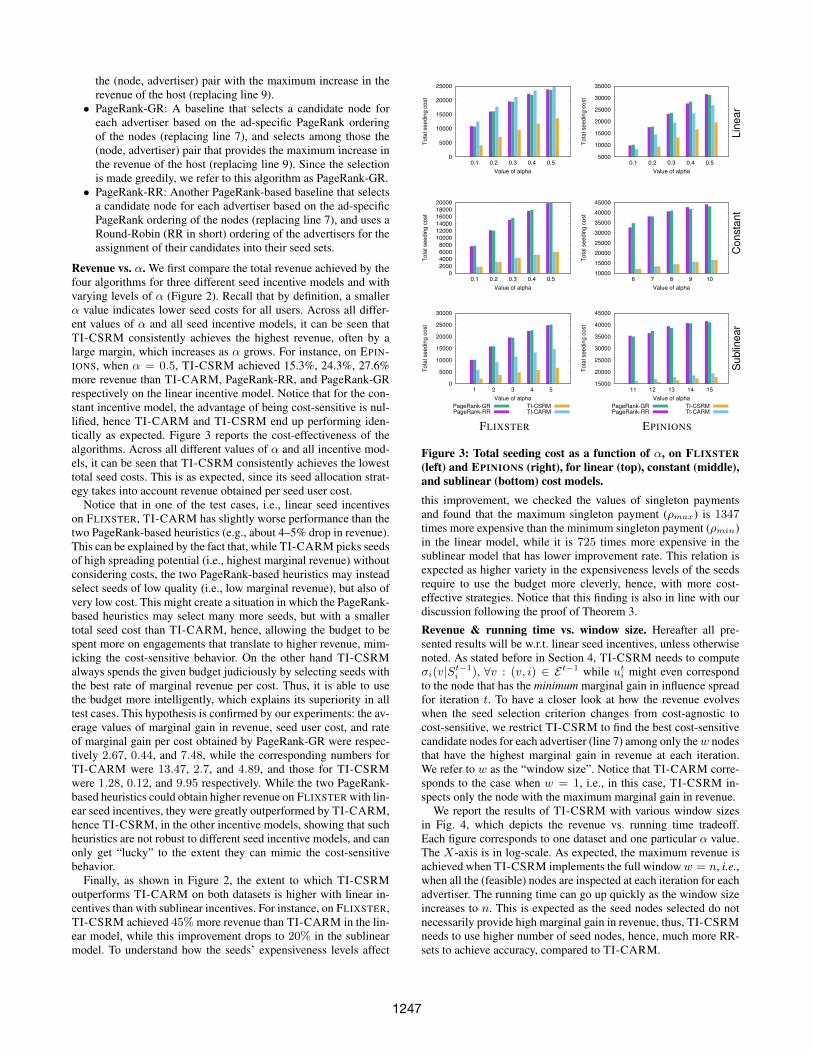
Revenue vs. α. We first compare the total revenue achieved by thefour algorithms for three different seed incentive models and withvarying levels of α (Figure 2). Recall that by definition, a smallerα value indicates lower seed costs for all users. Across all differ-ent values of α and all seed incentive models, it can be seen thatTI-CSRM consistently achieves the highest revenue, often by alarge margin, which increases as α grows. For instance, on EPIN-IONS, when α = 0.5, TI-CSRM achieved 15.3%, 24.3%, 27.6%more revenue than TI-CARM, PageRank-RR, and PageRank-GRrespectively on the linear incentive model. Notice that for the con-stant incentive model, the advantage of being cost-sensitive is nul-lified, hence TI-CARM and TI-CSRM end up performing iden-tically as expected. Figure 3 reports the cost-effectiveness of thealgorithms. Across all different values of α and all incentive mod-els, it can be seen that TI-CSRM consistently achieves the lowesttotal seed costs. This is as expected, since its seed allocation strat-egy takes into account revenue obtained per seed user cost.

Notice that in one of the test cases, i.e., linear seed incentiveson FLIXSTER, TI-CARM has slightly worse performance than thetwo PageRank-based heuristics (e.g., about 4–5% drop in revenue).This can be explained by the fact that, while TI-CARM picks seedsof high spreading potential (i.e., highest marginal revenue) withoutconsidering costs, the two PageRank-based heuristics may insteadselect seeds of low quality (i.e., low marginal revenue), but also ofvery low cost. This might create a situation in which the PageRank-based heuristics may select many more seeds, but with a smallertotal seed cost than TI-CARM, hence, allowing the budget to bespent more on engagements that translate to higher revenue, mim-icking the cost-sensitive behavior. On the other hand TI-CSRMalways spends the given budget judiciously by selecting seeds withthe best rate of marginal revenue per cost. Thus, it is able to usethe budget more intelligently, which explains its superiority in alltest cases. This hypothesis is confirmed by our experiments: the av-erage values of marginal gain in revenue, seed user cost, and rateof marginal gain per cost obtained by PageRank-GR were respec-tively 2.67, 0.44, and 7.48, while the corresponding numbers forTI-CARM were 13.47, 2.7, and 4.89, and those for TI-CSRMwere 1.28, 0.12, and 9.95 respectively. While the two PageRank-based heuristics could obtain higher revenue on FLIXSTER with lin-ear seed incentives, they were greatly outperformed by TI-CARM,hence TI-CSRM, in the other incentive models, showing that suchheuristics are not robust to different seed incentive models, and canonly get “lucky” to the extent they can mimic the cost-sensitivebehavior.

Finally, as shown in Figure 2, the extent to which TI-CSRMoutperforms TI-CARM on both datasets is higher with linear in-centives than with sublinear incentives. For instance, on FLIXSTER,TI-CSRM achieved 45% more revenue than TI-CARM in the lin-ear model, while this improvement drops to 20% in the sublinearmodel. To understand how the seeds’ expensiveness levels affect

0

5000

10000

15000

20000

25000

0.1 0.2 0.3 0.4 0.5

Tota

l see

ding

cos

t

Value of alpha

5000

10000

15000

20000

25000

30000

35000

0.1 0.2 0.3 0.4 0.5

Tota

l see

ding

cos

t

Value of alpha

Line

ar

0 2000 4000 6000 8000

10000 12000 14000 16000 18000 20000

0.1 0.2 0.3 0.4 0.5

Tota

l see

ding

cos

t

Value of alpha

10000 15000 20000 25000 30000 35000 40000 45000

6 7 8 9 10

Tota

l see

ding

cos

t

Value of alpha

Con

stan

t

0

5000

10000

15000

20000

25000

30000

1 2 3 4 5

Tota

l seedin

g c

ost

Value of alpha

PageRank-RRPageRank-GR

TI-CARMTI-CSRM

15000

20000

25000

30000

35000

40000

45000

11 12 13 14 15

Tota

l seedin

g c

ost

Value of alpha

PageRank-RRPageRank-GR

TI-CARMTI-CSRM

Sub

linea

r

FLIXSTER EPINIONS

Figure 3: Total seeding cost as a function of α, on FLIXSTER(left) and EPINIONS (right), for linear (top), constant (middle),and sublinear (bottom) cost models.this improvement, we checked the values of singleton paymentsand found that the maximum singleton payment (ρmax) is 1347times more expensive than the minimum singleton payment (ρmin)in the linear model, while it is 725 times more expensive in thesublinear model that has lower improvement rate. This relation isexpected as higher variety in the expensiveness levels of the seedsrequire to use the budget more cleverly, hence, with more cost-effective strategies. Notice that this finding is also in line with ourdiscussion following the proof of Theorem 3.

Revenue & running time vs. window size. Hereafter all pre-sented results will be w.r.t. linear seed incentives, unless otherwisenoted. As stated before in Section 4, TI-CSRM needs to computeσi(v|St−1

i ), ∀v : (v, i) ∈ Et−1 while uti might even correspondto the node that has the minimum marginal gain in influence spreadfor iteration t. To have a closer look at how the revenue evolveswhen the seed selection criterion changes from cost-agnostic tocost-sensitive, we restrict TI-CSRM to find the best cost-sensitivecandidate nodes for each advertiser (line 7) among only thew nodesthat have the highest marginal gain in revenue at each iteration.We refer to w as the “window size”. Notice that TI-CARM corre-sponds to the case when w = 1, i.e., in this case, TI-CSRM in-spects only the node with the maximum marginal gain in revenue.

We report the results of TI-CSRM with various window sizesin Fig. 4, which depicts the revenue vs. running time tradeoff.Each figure corresponds to one dataset and one particular α value.The X-axis is in log-scale. As expected, the maximum revenue isachieved when TI-CSRM implements the full windoww = n, i.e.,when all the (feasible) nodes are inspected at each iteration for eachadvertiser. The running time can go up quickly as the window sizeincreases to n. This is expected as the seed nodes selected do notnecessarily provide high marginal gain in revenue, thus, TI-CSRMneeds to use higher number of seed nodes, hence, much more RR-sets to achieve accuracy, compared to TI-CARM.

1247

36000

38000

40000

42000

44000

46000

48000

110 1100

Tota

l Rev

enue

Average Running Time (sec)

1

50

100

250

500

1000

2500

5000

N

28000 30000 32000 34000 36000 38000 40000

80 800

Tota

l Rev

enue

Average Running Time (sec)

1

50

100

250

500

1000

2500

5000

N

69000 70000 71000 72000 73000 74000 75000 76000

40 400

Tota

l Rev

enue

Average Running Time (sec)

1

50

100

250

500

1000

2500

5000

N

56000

58000

60000

62000

64000

66000

40 400

Tota

l Rev

enue

Average Running Time (sec)

1

50

100

250

500

1000

2500

5000

N

(a) FLIXSTER (α = 0.2) (b) FLIXSTER (α = 0.5) (c) EPINIONS (α = 0.2) (d) EPINIONS (α = 0.5)

Figure 4: Revenue vs running time tradeoff on FLIXSTER and EPINIONS for two different value of α.

Table 3: Memory usage (GB).DBLP h = 1 5 10 15 20

TI-CARM 1.6 7.5 14.9 22.4 29.8TI-CSRM (5000) 1.6 7.6 15.1 22.7 30.2LIVEJOURNAL h = 1 5 10 15 20

TI-CARM 2.5 12.1 25.3 39.4 54.4TI-CSRM (5000) 3.4 15.9 31.2 49.1 67.5

Scalability. We tested the scalability of TI-CARM and TI-CSRMon two larger graphs, DBLP and LIVEJOURNAL. In all scalabil-ity experiments, we use a window size of w = 5000 nodes forTI-CSRM due to its good revenue vs running time trade-off. Forsimplicity, all CPEs were set to 1. The influence probability oneach edge (u, v) ∈ E was computed using the Weighted-Cascademodel [24], where piu,v = 1/|N in(v)| for all ads i. We set α = 0.2and ε = 0.3. This setting is well-suited for testing scalability as itsimulates a fully competitive case: all advertisers compete for thesame set of influential users (due to all ads having the same distri-bution over the topics), and hence it will “stress-test” the algorithmsby prolonging the seed selection process.

Figure 5(a) and 5(b) depict the running time of TI-CARM andTI-CSRM as the number of advertisers goes up from 1 to 20, whilethe budget is fixed (10K for DBLP and 100K for LIVEJOURNAL).As can be seen, the running time increases mostly in a linear man-ner, and TI-CSRM is only slightly slower than TI-CARM. Fig-ure 5(c) and 5(d) depict the running time of TI-CARM and TI-CSRM as the budget increases, while the number of advertisers isfixed at h = 5 . We can also see that the increasing trend is mostlylinear for TI-CSRM, while TI-CARM’s time goes in a flatter fash-ion. All in all, both algorithms exhibit decent scalability.

Table 3 shows the memory usage of TI-CARM and TI-CSRMwhen h increases. TI-CSRM in general needs to use higher mem-ory than TI-CARM due to its requirement to generate more RRsets that ensures accuracy for using higher seed set size than TI-CARM. On DBLP, TI-CARM and TI-CSRM respectively usesa total of 4676 and 7276 seed nodes for h = 20. On LIVEJOURNALTI-CSRM used typically between 20% to 40% more memory thanTI-CARM: TI-CARM and TI-CSRM respectively uses a total of4327 and 6123 seed nodes for h = 20.

6. RELATED WORKComputational advertising. Considerable work has been donein sponsored search and display ads [18–21, 28, 30]. In sponsoredsearch, revenue maximization is formalized as the well-known Ad-words problem [29]. Given a set of keywords and bidders with theirdaily budgets and bids for each keyword, words need to be assignedto bidders upon arrival, to maximize the revenue for the day, whilerespecting bidder budgets. This can be solved with a competitiveratio of (1− 1/e) [29].Social advertising. In comparison with computational advertis-ing, social advertising is in its infancy. Recent efforts, including

Tucker [35] and Bakshy et al. [5], have shown, by means of fieldstudies on sponsored posts in Facebook’s News Feed, the impor-tance of taking social influence into account when developing so-cial advertising strategies. However, literature on exploiting socialinfluence for social advertising is rather limited. Bao and Changhave proposed AdHeat [7], a social ad model considering socialinfluence in addition to relevance for matching ads to users. Theirexperiments show that AdHeat significantly outperforms the rele-vance model on click-through-rate (CTR). Wang et al. [36] proposea new model for learning relevance and apply it for selecting rele-vant ads for Facebook users. Neither of these works studies viralad propagation or revenue maximization.

Chalermsook et al. [12] study revenue maximization for the host,when dealing with multiple advertisers. In their setting, each ad-vertiser pays the host an amount for each product adoption, up toa budget. In addition, each advertiser also specifies the maximumsize of its seed set. This additional constraint considerably simpli-fies the problem compared to our setting, where the absence of aprespecified seed set size is a significant challenge.

Aslay et al. [4] study regret minimization for a host supportingcampaigns from multiple advertisers. Here, regret is the differencebetween the monetary budget of an advertiser and the value of ex-pected number of engagements achieved by the campaign, based onthe CPE pricing model. They share with us the pricing model andadvertiser budget. However, they do not consider seed user costs.Besides they attack a very different optimization problem and theiralgorithms and results do not carry over to our setting.

Abbassi et al. [2] study a cost-per-mille (CPM) model in displayadvertising. The host enters into a contract with each advertiser toshow their ad to a fixed number of users, for an agreed upon CPMamount per thousand impressions. The problem is that of selectingthe sequence of users to show the ads to, in order to maximize theexpected number of clicks. This is a substantially different problemwhich they show is APX-hard and propose heuristic solutions.

Alon et al. [3] study budget allocation among channels and influ-ential customers, with the intuition that a channel assigned a higherbudget will make more attempts at influencing customers. They donot take into account viral propagation. Their main result is that forsome influence models the budget allocation problem can be ap-proximated, while for others it is inapproximable. Notably, none ofthese previous works studies incentivized social advertising wherethe seed users are paid monetary incentives.

Viral marketing. Kempe et al. [24] formalize the influence max-imization problem which requires to select k seed nodes, where kis a cardinality budget, such that the expected spread of influencefrom the selected seeds is maximized. Of particular note are the re-cent advances (already reviewed in Section 4) that have been madein designing scalable approximation algorithms [10, 14, 32–34] forthis hard problem. Numerous variants of the influence maximiza-tion problem have been studied over the years, including compe-tition [9, 11], host perspective [4, 27], non-uniform cost model for

1248

0

200

400

600

800

1000

1200

1400

1 5 10 15 20

Runnin

g T

ime (

sec)

Number of Advertisers

TI-CSRM (5000)TI-CARM

0

2000

4000

6000

8000

10000

12000

14000

1 5 10 15 20

Runnin

g T

ime (

sec)

Number of Advertisers

TI-CSRM (5000)TI-CARM

0

100

200

300

400

500

600

5 10 15 20 25 30

Runnin

g T

ime (

sec)

Budget (x1000)

TI-CSRM (5000)TI-CARM

2600

2800

3000

3200

3400

3600

3800

4000

4200

4400

50 100 150 200 250

Runnin

g T

ime (

sec)

Budget (x1000)

TI-CSRM (5000)TI-CARM

(a) DBLP (h) (b) LIVEJOURNAL (h) (c) DBLP (budgets) (d) LIVEJOURNAL (budgets)

Figure 5: Running time of TI-CARM and TI-CSRM on DBLP and LIVEJOURNAL

seed users [26, 31], and fractional seed selection [17]. However, toour knowledge, there has been no previous work that addresses in-centivized social advertising, while leveraging viral propagation ofsocial ads and handling advertiser budgets.

7. CONCLUSIONSIn this paper, we initiate the investigation of incentivized social

advertising, by formalizing the fundamental problem of revenuemaximization from the host perspective. In our formulation, incen-tives paid to the seed users are determined by their demonstratedpast influence in the topic of the specific ad. We show that, keep-ing all important factors – topical relevance of ads, their propensityfor social propagation, the topical influence of users, seed users’incentives, and advertiser budgets – in consideration, the problemof revenue maximization in incentivized social advertising is NP-hard and it corresponds to the problem of monotone submodularfunction maximization subject to a partition matroid constraint onthe ads-to-seeds allocation and multiple submodular knapsack con-straints on the advertiser budgets. For this problem, we devise twonatural greedy algorithms that differ in their sensitivity to seeduser incentive costs, provide formal approximation guarantees, andachieve scalability by adapting to our context recent advances madein scalable estimation of expected influence spread.

Our work takes an important first step toward enriching theframework of incentivized social advertising with powerful ideasfrom viral marketing, while making the latter more applicable toreal-world online marketing. It opens up several interesting avenuesfor further research: (i) it remains open whether our winning algo-rithm TI-CSRM can be made more memory efficient hence morescalable; (ii) it remains open whether the approximation bound forCS-GREEDY provided in Theorem 3 is tight; (iii) it is interestingto integrate hard competition constraints into the influence propa-gation process; (iv) it is worth studying our problem in an onlineadaptive setting where the partial results of the campaign can betaken into account while deciding the next moves. All these direc-tions offer a wealth of possibilities for future work.

8. REFERENCES[1] https://arxiv.org/abs/1612.00531.[2] Z. Abbassi, A. Bhaskara, and V. Misra. Optimizing display advertising in

online social networks. In WWW 2015.[3] N. Alon, I. Gamzu, and M. Tennenholtz. Optimizing budget allocation among

channels and influencers. In WWW 2012.[4] C. Aslay, W. Lu, F. Bonchi, A. Goyal, and L. V. S. Lakshmanan. Viral

marketing meets social advertising: Ad allocation with minimum regret.PVLDB, 8(7):822–833, 2015.

[5] E. Bakshy, D. Eckles, R. Yan, and I. Rosenn. Social influence in socialadvertising: evidence from field experiments. In EC 2012.

[6] E. Bakshy, J. M. Hofman, W. A. Mason, and D. J. Watts. Everyone’s aninfluencer: quantifying influence on twitter. In WSDM 2011.

[7] H. Bao and E. Y. Chang. Adheat: An influence-based diffusion model forpropagating hints to match ads. In WWW 2010.

[8] N. Barbieri, F. Bonchi, and G. Manco. Topic-aware social influencepropagation models. In ICDM 2012.

[9] S. Bharathi, D. Kempe, and M. Salek. Competitive influence maximization insocial networks. In WINE 2007.

[10] C. Borgs, M. Brautbar, J. T. Chayes, and B. Lucier. Maximizing socialinfluence in nearly optimal time. In SODA 2014.

[11] T. Carnes, C. Nagarajan, S. M. Wild, and A. van Zuylen. Maximizing influencein a competitive social network: a follower’s perspective. In ICEC 2007.

[12] P. Chalermsook, A. D. Sarma, A. Lall, and D. Nanongkai. Social networkmonetization via sponsored viral marketing. In SIGMETRICS 2015.

[13] W. Chen, C. Wang, and Y. Wang. Scalable influence maximization forprevalent viral marketing in large-scale social networks. In KDD 2010.

[14] E. Cohen, D. Delling, T. Pajor, , and R. F. Werneck. Sketch-based influencemaximization and computation: Scaling up with guarantees. In CIKM 2014.

[15] M. Conforti and G. Cornuejols. Submodular set functions, matroids and thegreedy algorithm: tight worst-case bounds and some generalizations of therado-edmonds theorem. Discrete applied mathematics, 7(3):251–274, 1984.

[16] P. Dagum, R. Karp, M. Luby, and S. Ross. An optimal algorithm for montecarlo estimation. SIAM Journal on computing, 29(5):1484–1496, 2000.

[17] E. D. Demaine, M. Hajiaghayi, H. Mahini, D. L. Malec, S. Raghavan,A. Sawant, and M. Zadimoghaddam. How to influence people with partialincentives. In WWW 2014.

[18] N. R. Devanur, B. Sivan, and Y. Azar. Asymptotically optimal algorithm forstochastic adwords. In EC 2012.

[19] J. Feldman, M. Henzinger, N. Korula, V. S. Mirrokni, and C. Stein. Onlinestochastic packing applied to display ad allocation. In ESA 2010.

[20] J. Feldman, N. Korula, V. S. Mirrokni, S. Muthukrishnan, and M. Pal. Onlinead assignment with free disposal. In WINE 2009.

[21] G. Goel and A. Mehta. Online budgeted matching in random input modelswith applications to adwords. In SODA 2008.

[22] R. Iyer. Submodular Optimization and Machine Learning: Theoretical Results,Unifying and Scalable Algorithms, and Applications. PhD thesis, Univ. ofWashington, 2015.

[23] R. K. Iyer and J. A. Bilmes. Submodular optimization with submodular coverand submodular knapsack constraints. In NIPS 2013.

[24] D. Kempe, J. M. Kleinberg, and E. Tardos. Maximizing the spread of influencethrough a social network. In KDD 2003.

[25] B. Korte and D. Hausmann An analysis of the greedy heuristic forindependence systems. In Annals of Discrete Mathematics 1978.

[26] J. Leskovec, A. Krause, C. Guestrin, C. Faloutsos, J. M. VanBriesen, and N. S.Glance. Cost-effective outbreak detection in networks. In KDD 2007.

[27] W. Lu, F. Bonchi, A. Goyal, and L. V. Lakshmanan. The bang for the buck:fair competitive viral marketing from the host perspective. In KDD 2013.

[28] A. Mehta. Online matching and ad allocation. Foundations and Trends inTheoretical Computer Science, 8(4):265–368, 2013.

[29] A. Mehta, A. Saberi, U. V. Vazirani, and V. V. Vazirani. Adwords andgeneralized online matching. J. ACM, 54(5), 2007.

[30] V. S. Mirrokni, S. O. Gharan, and M. Zadimoghaddam. Simultaneousapproximations for adversarial and stochastic online budgeted allocation. InSODA 2012.

[31] H. Nguyen and R. Zheng. On budgeted influence maximization in socialnetworks. IEEE Journal on Selected Areas in Communications,31(6):1084–1094, 2013.

[32] H. T. Nguyen, M. T. Thai, and T. N. Dinh. Stop-and-stare: Optimal samplingalgorithms for viral marketing in billion-scale networks. In SIGMOD 2016.

[33] Y. Tang, Y. Shi, and X. Xiao. Influence maximization in near-linear time: Amartingale approach. In SIGMOD 2015.

[34] Y. Tang, X. Xiao, and Y. Shi. Influence maximization: Near-optimal timecomplexity meets practical efficiency. SIGMOD 2014.

[35] C. Tucker. Social advertising. Available at SSRN 1975897, 2012.[36] C. Wang, R. Raina, D. Fong, D. Zhou, J. Han, and G. Badros. Learning

relevance from heterogeneous social network and its application in onlinetargeting. In SIGIR 2011.

1249