Expectation Maximization Machine Learning. Last Time Expectation Maximization Gaussian Mixture...
33
Expectation Maximization Machine Learning
-
Upload
keira-janeway -
Category
Documents
-
view
231 -
download
1
Transcript of Expectation Maximization Machine Learning. Last Time Expectation Maximization Gaussian Mixture...
Expectation Maximization
Machine Learning
Last Time
• Expectation Maximization• Gaussian Mixture Models
Today
• EM Proof– Jensen’s Inequality
• Clustering sequential data– EM over HMMs– EM in any Graphical Model• Gibbs Sampling
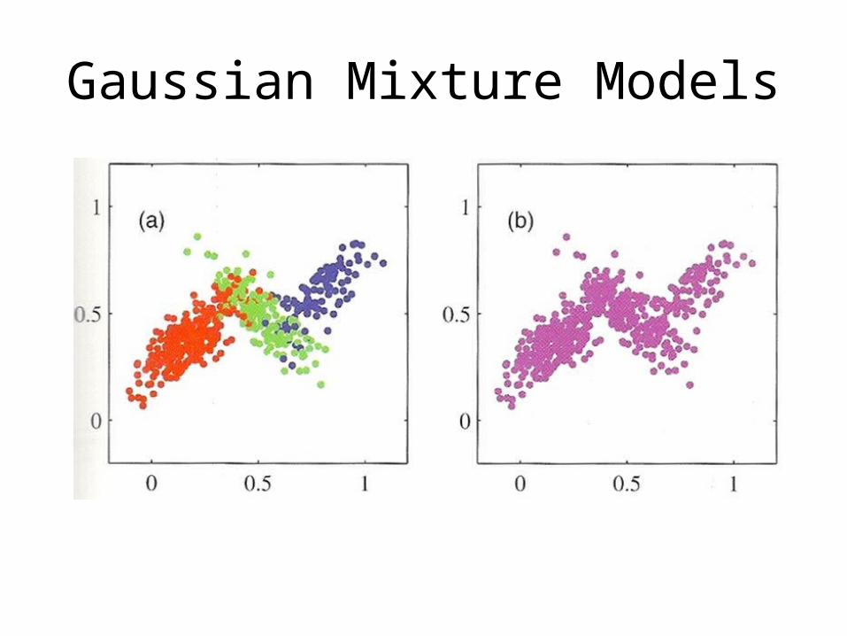
Gaussian Mixture Models
How can we be sure GMM/EM works?
• We’ve already seen that there are multiple clustering solutions for the same data.– Non-convex optimization problem
• Can we prove that we’re approaching some maximum, even if many exist.
Bound maximization
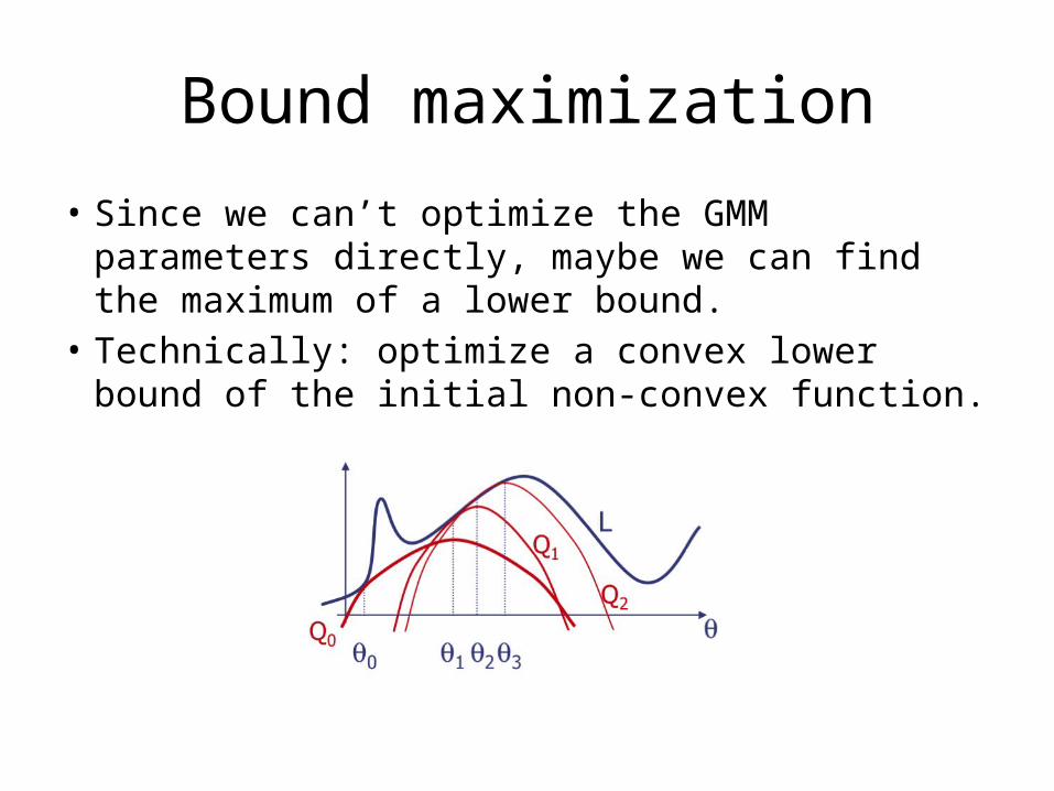
• Since we can’t optimize the GMM parameters directly, maybe we can find the maximum of a lower bound.
• Technically: optimize a convex lower bound of the initial non-convex function.
EM as a bound maximization problem
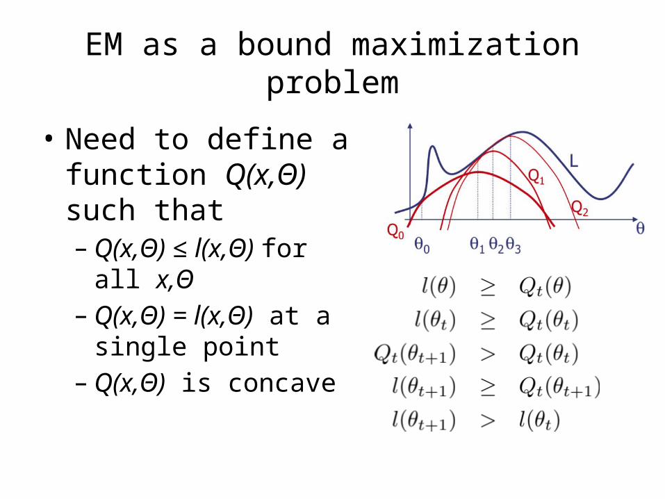
• Need to define a function Q(x,Θ) such that– Q(x,Θ) ≤ l(x,Θ) for all x,Θ– Q(x,Θ) = l(x,Θ) at a single
point– Q(x,Θ) is concave

EM as bound maximization
• Claim: – for GMM likelihood
– The GMM MLE estimate is a convex lower bound
EM Correctness Proof
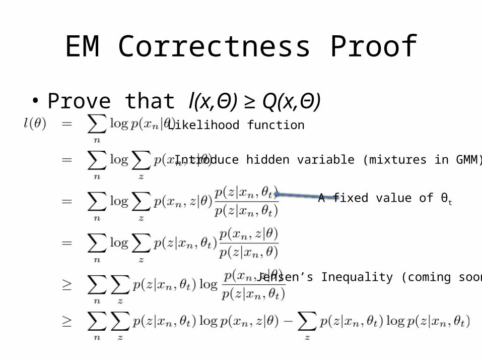
• Prove that l(x,Θ) ≥ Q(x,Θ)Likelihood function
Introduce hidden variable (mixtures in GMM)
A fixed value of θt
Jensen’s Inequality (coming soon…)

EM Correctness Proof
GMM Maximum Likelihood Estimation
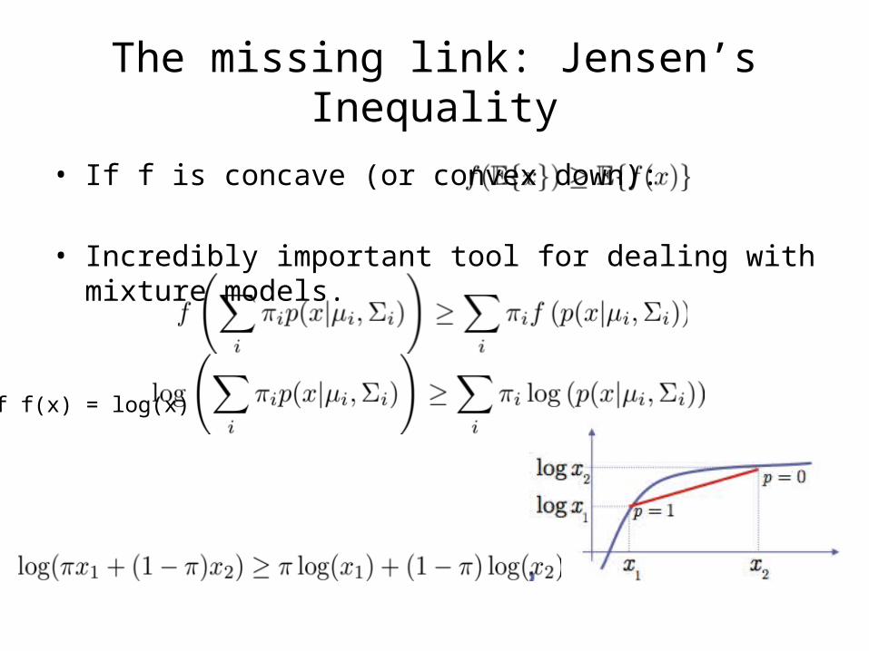
The missing link: Jensen’s Inequality
• If f is concave (or convex down):
• Incredibly important tool for dealing with mixture models.
if f(x) = log(x)
Generalizing EM from GMM
• Notice, the EM optimization proof never introduced the exact form of the GMM
• Only the introduction of a hidden variable, z.• Thus, we can generalize the form of EM to
broader types of latent variable models
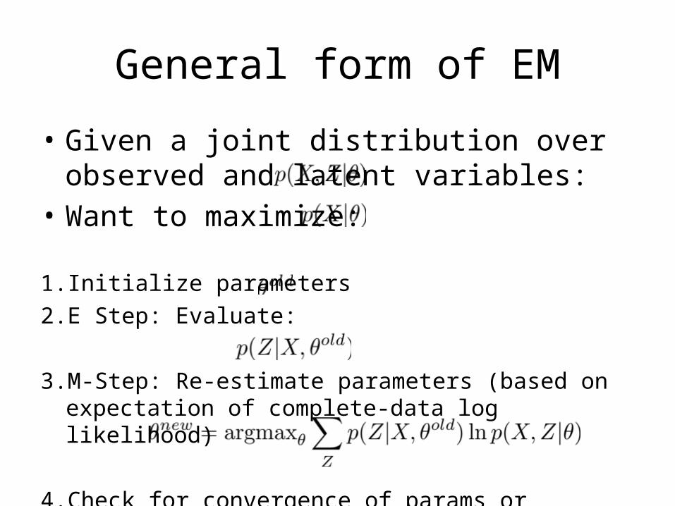
General form of EM
• Given a joint distribution over observed and latent variables:
• Want to maximize:
1. Initialize parameters2. E Step: Evaluate:
3. M-Step: Re-estimate parameters (based on expectation of complete-data log likelihood)
4. Check for convergence of params or likelihood
Applying EM to Graphical Models
• Now we have a general form for learning parameters for latent variables.– Take a Guess– Expectation: Evaluate likelihood– Maximization: Reestimate parameters– Check for convergence
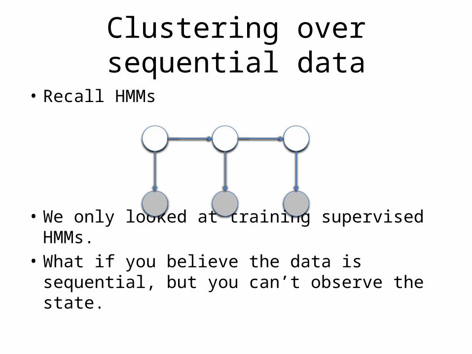
Clustering over sequential data
• Recall HMMs
• We only looked at training supervised HMMs.• What if you believe the data is sequential, but
you can’t observe the state.
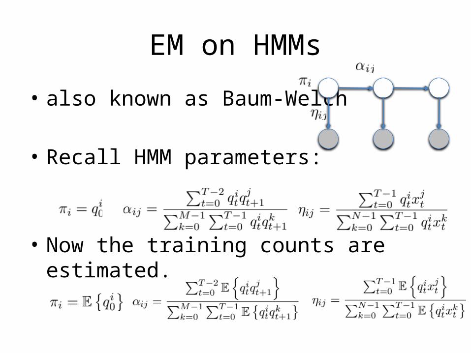
EM on HMMs
• also known as Baum-Welch
• Recall HMM parameters:
• Now the training counts are estimated.
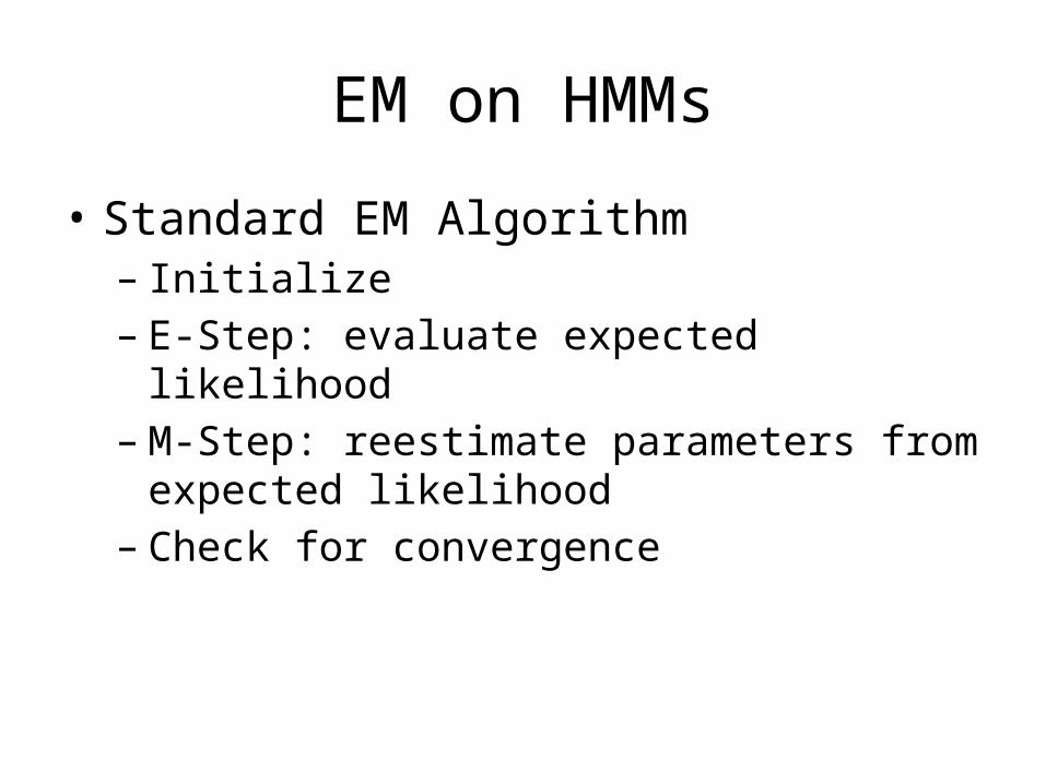
EM on HMMs
• Standard EM Algorithm– Initialize– E-Step: evaluate expected likelihood– M-Step: reestimate parameters from expected
likelihood– Check for convergence
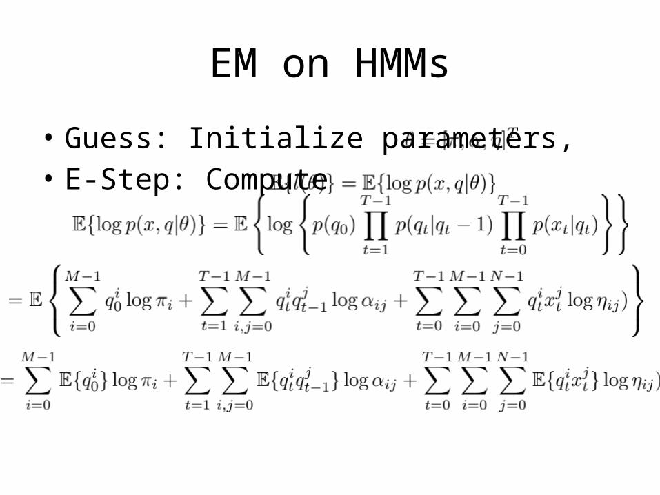
EM on HMMs
• Guess: Initialize parameters, • E-Step: Compute
EM on HMMs
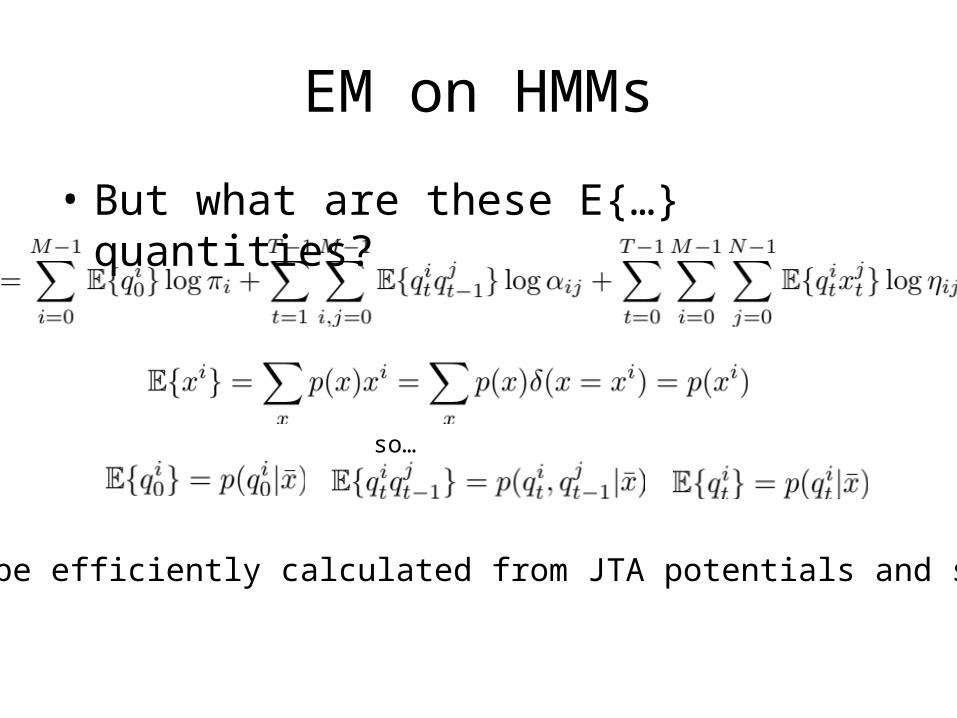
• But what are these E{…} quantities?
so…
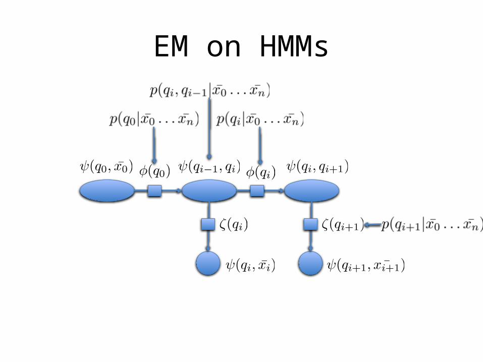
These can be efficiently calculated from JTA potentials and separators.
EM on HMMs
EM on HMMs
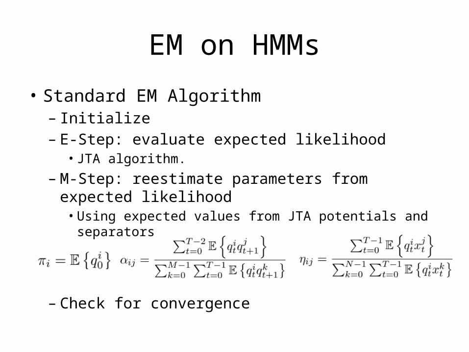
• Standard EM Algorithm– Initialize– E-Step: evaluate expected likelihood
• JTA algorithm.
– M-Step: reestimate parameters from expected likelihood• Using expected values from JTA potentials and separators
– Check for convergence
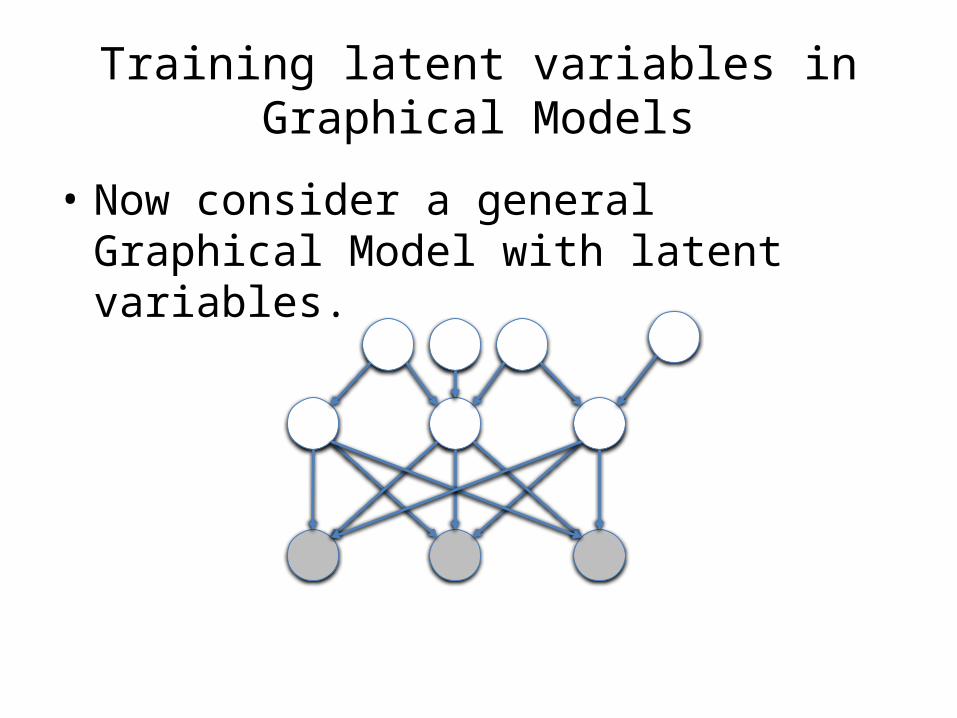
Training latent variables in Graphical Models
• Now consider a general Graphical Model with latent variables.
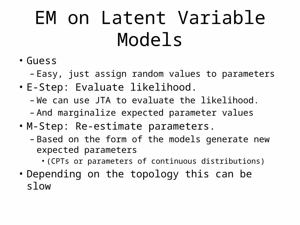
EM on Latent Variable Models
• Guess– Easy, just assign random values to parameters
• E-Step: Evaluate likelihood.– We can use JTA to evaluate the likelihood.– And marginalize expected parameter values
• M-Step: Re-estimate parameters.– Based on the form of the models generate new
expected parameters • (CPTs or parameters of continuous distributions)
• Depending on the topology this can be slow
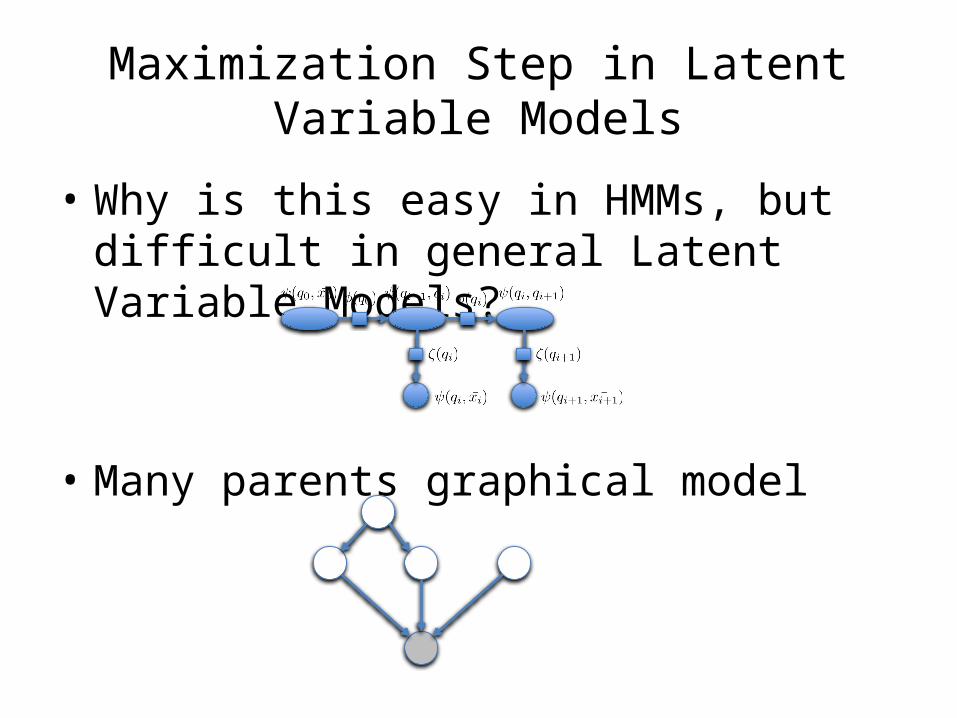
Maximization Step in Latent Variable Models
• Why is this easy in HMMs, but difficult in general Latent Variable Models?
• Many parents graphical model
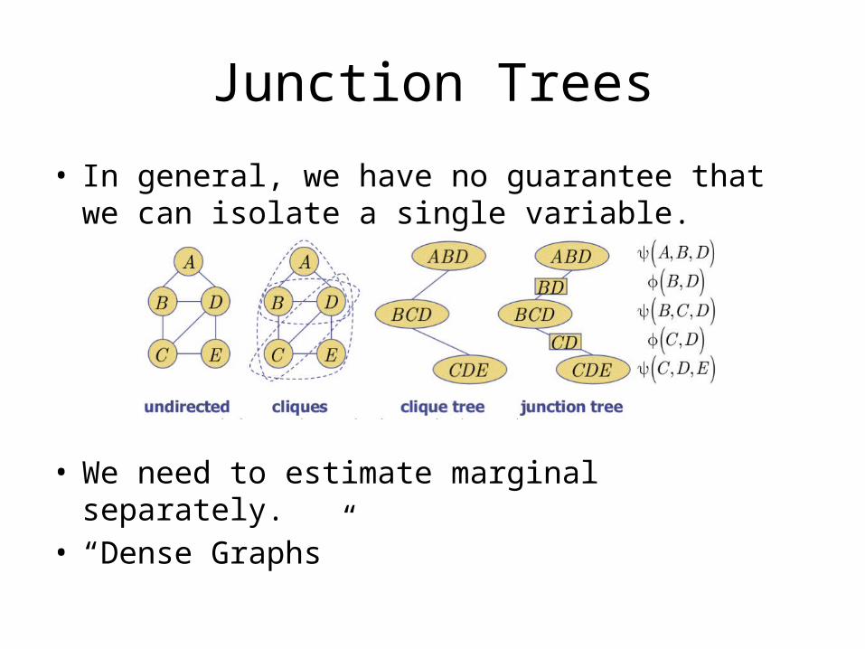
Junction Trees
• In general, we have no guarantee that we can isolate a single variable.
• We need to estimate marginal separately.• “Dense Graphs”
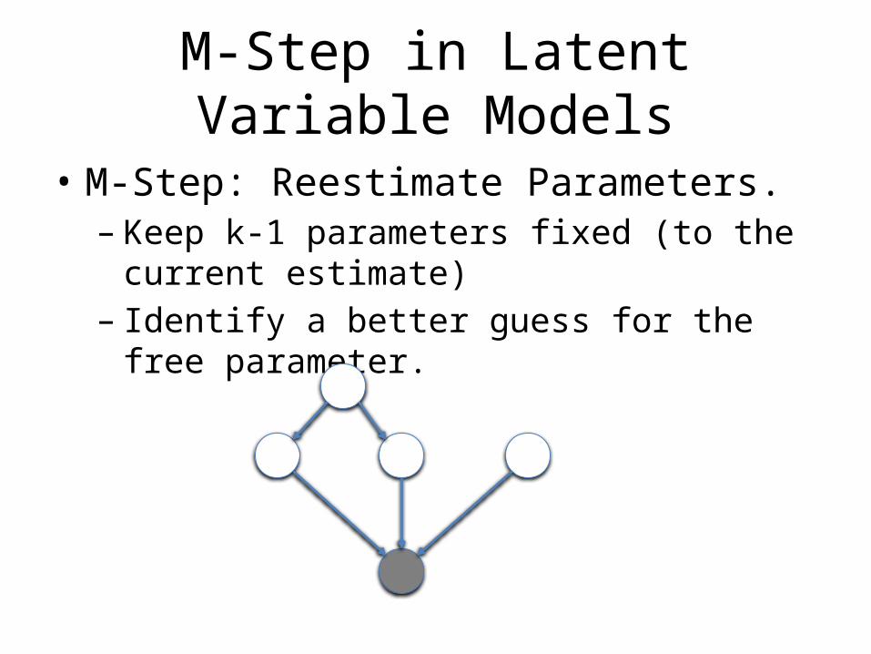
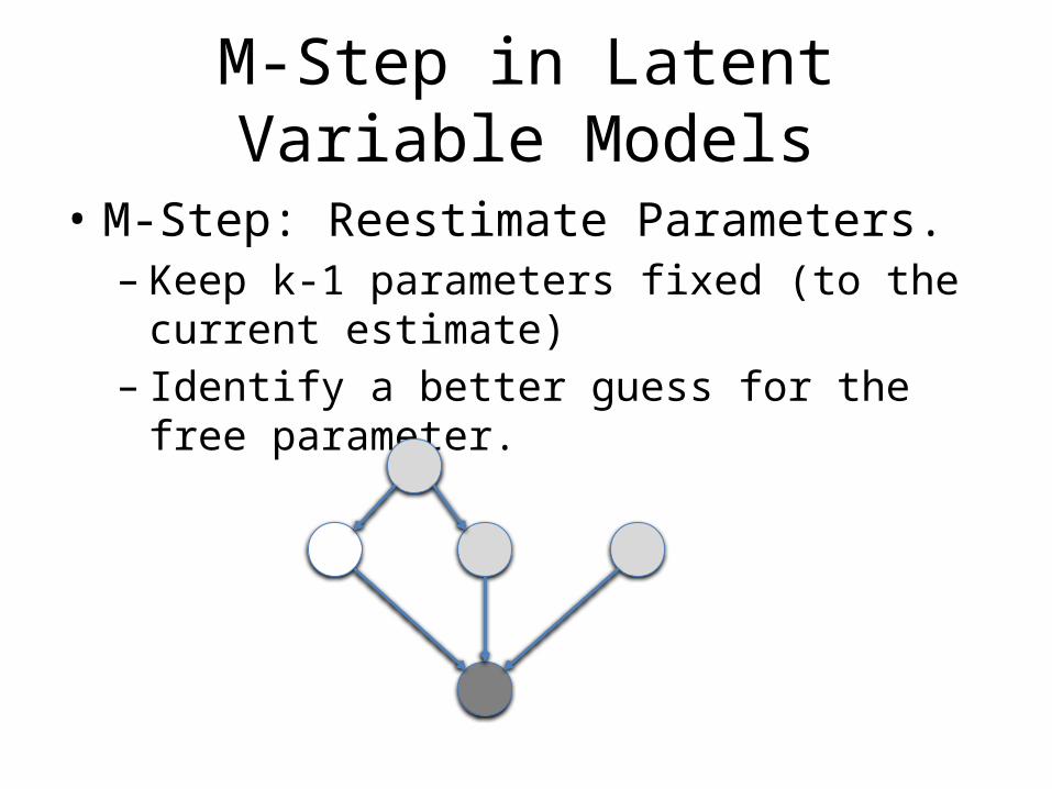
M-Step in Latent Variable Models
• M-Step: Reestimate Parameters.– Keep k-1 parameters fixed (to the current
estimate)– Identify a better guess for the free parameter.
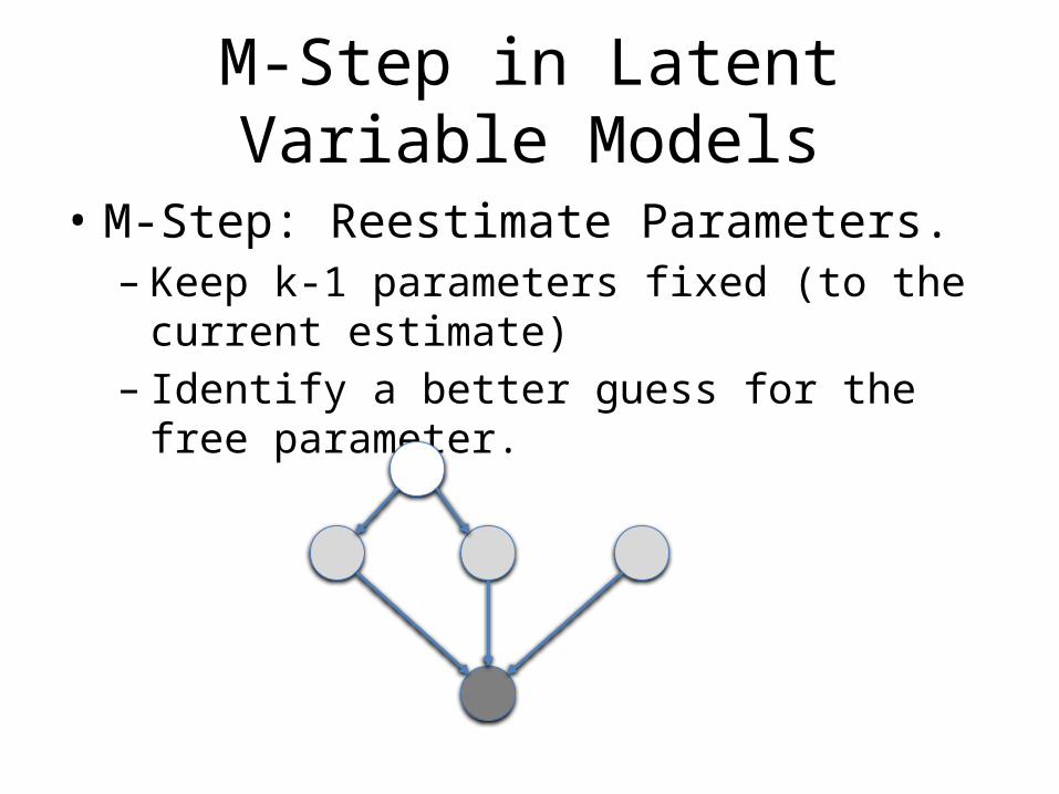
M-Step in Latent Variable Models
• M-Step: Reestimate Parameters.– Keep k-1 parameters fixed (to the current
estimate)– Identify a better guess for the free parameter.
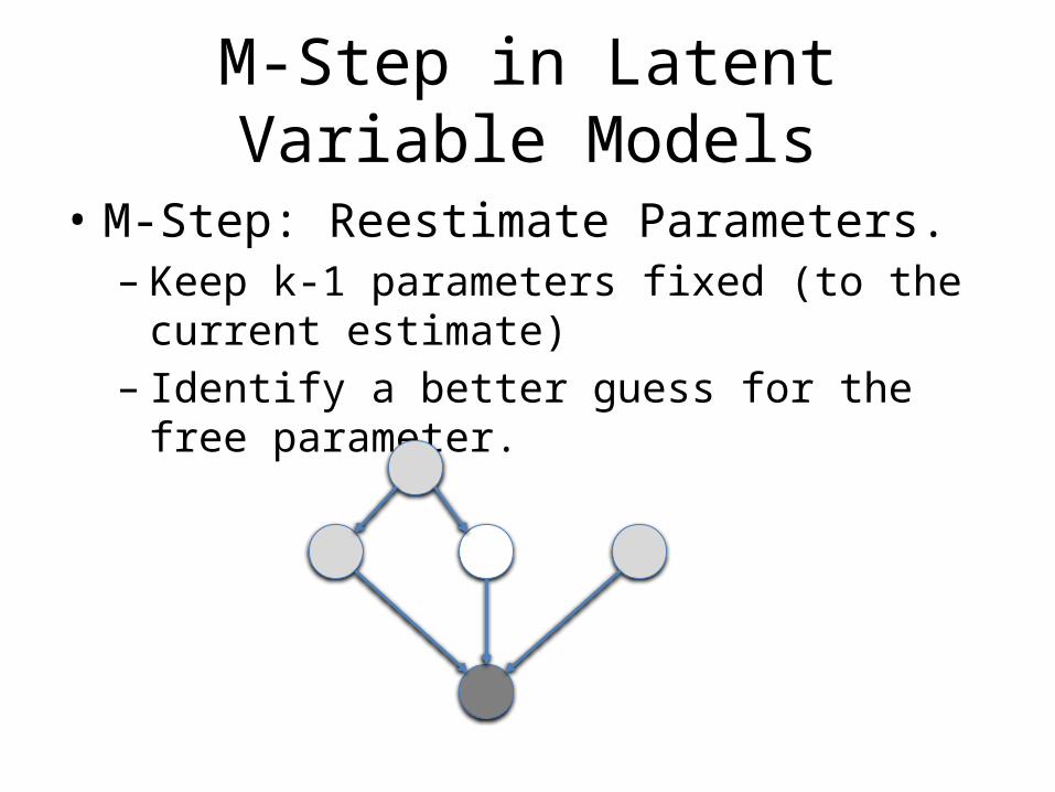
M-Step in Latent Variable Models
• M-Step: Reestimate Parameters.– Keep k-1 parameters fixed (to the current
estimate)– Identify a better guess for the free parameter.
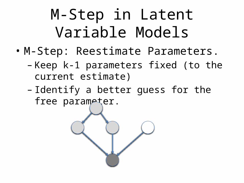
M-Step in Latent Variable Models
• M-Step: Reestimate Parameters.– Keep k-1 parameters fixed (to the current
estimate)– Identify a better guess for the free parameter.
M-Step in Latent Variable Models
• M-Step: Reestimate Parameters.– Keep k-1 parameters fixed (to the current
estimate)– Identify a better guess for the free parameter.
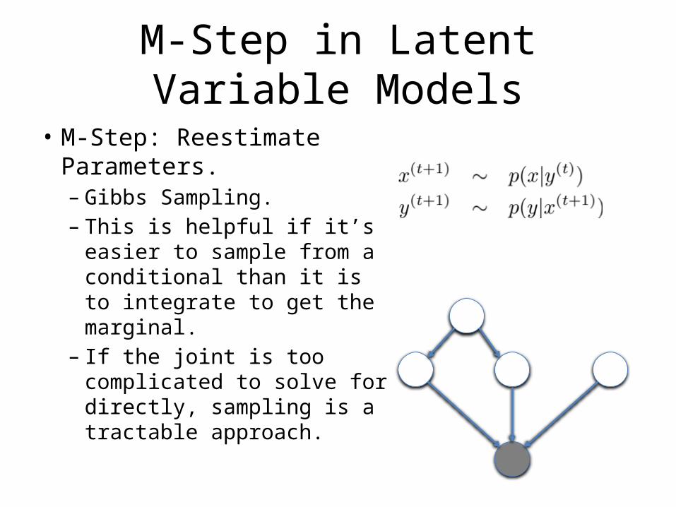
M-Step in Latent Variable Models
• M-Step: Reestimate Parameters.– Gibbs Sampling.– This is helpful if it’s easier to
sample from a conditional than it is to integrate to get the marginal.
– If the joint is too complicated to solve for directly, sampling is a tractable approach.
EM on Latent Variable Models
• Guess– Easy, just assign random values to parameters
• E-Step: Evaluate likelihood.– We can use JTA to evaluate the likelihood.– And marginalize expected parameter values
• M-Step: Re-estimate parameters.– Either JTA potentials and marginals
• Or don’t do EM and Sample…
Break
• Unsupervised Feature Selection– Principle Component Analysis