Return distributions and volatility forecasting in metal ...

The authors are grateful to Nancy Jianakoplos, Charles Revier, and Deepankar Basu for their helpful adviceon this research. We also wish to thank the editor, Bob Webb, and an anonymous reviewer for their thought-ful and constructive comments. The authors are responsible for any remaining errors.

*Correspondence author, Department of Finance and Real Estate, Colorado State University, Fort Collins,Colorado 80523. Tel: (970) 491-6681, e-mail: [email protected]

Received August 2009; Accepted January 2010

■ Ahmed A. A. Khalifa is in the Department of Economics, Bloomsburg University ofPennsylvania, Bloomsburg, Pennsylvania.

■ Hong Miao and Sanjay Ramchander are in the Department of Finance and Real Estate,Colorado State University, Fort Collins, Colorado.

The Journal of Futures Markets, Vol. 31, No. 1, 55–80 (2011)© 2010 Wiley Periodicals, Inc.Published online March 29, 2010 in Wiley Online Library (wileyonlinelibrary.com).DOI: 10.1002/fut.20459

RETURN DISTRIBUTIONS AND

VOLATILITY FORECASTING IN

METAL FUTURES MARKETS:EVIDENCE FROM GOLD, SILVER,AND COPPER

AHMED A. A. KHALIFAHONG MIAOSANJAY RAMCHANDER*

The characterization of return distributions and forecast of asset-price variabilityplay a critical role in the study of financial markets. This study estimates fourmeasures of integrated volatility—daily absolute returns, realized volatility, real-ized bipower volatility, and integrated volatility via Fourier transformation(IVFT)—for gold, silver, and copper by using high-frequency data for the period1999 through 2008. The distributional properties are investigated by applyingrecently developed jump detection procedures and by constructing financial-timereturn series. The predictive ability of a GARCH (1, 1) forecasting model thatuses various volatility measures is also examined. Three important findings are

reported. First, the magnitude of the IVFT volatility estimate is the greatestamong the four volatility measures. Second, the return distributions of the threemarkets are not normal. However, when returns are standardized by IVFT andrealized volatility, the corresponding return distributions bear closer resemblanceto a normal distribution. Notably, the application of financial-time sampling tech-nique is helpful in obtaining a normal distribution. Finally, the IVFT and realizedvolatility proxies produce the smallest forecasting errors, and increasing the timefrequency of estimating integrated volatility does not necessarily improve forecastaccuracy. © 2010 Wiley Periodicals, Inc. Jrl Fut Mark 31:55–80, 2011

INTRODUCTION

Volatility modeling is the subject of extensive investigation in the financial eco-nomics literature (see, for instance, Andersen, Bollerslev, & Diebold, 2005;Andersen, Diebold, Labys, & Bollerslev, 2001; Figlewski, 1997; Poon &Granger, 2003). The measurement and forecasting of volatility is essential forthe characterization of market dynamics, valuation of assets, pricing of deriva-tive instruments, and choices that affect portfolio allocation decisions.Furthermore, policy makers, including central banks often rely on volatilityestimates to assess the vulnerability of financial markets and the economy.

The increased availability of high-frequency data has led to a renewed inter-est in understanding the return distribution properties, and developing new andimproved volatility measurements that make use of information available in intra-day prices. As a result various volatility measures have been examined in studiesthat provide fresh insights related to the distributional properties and dynamicdependencies in financial markets (for example, Andersen & Bollerslev, 1998a;Andersen, Bollerslev, Frederiksen, & Nielsen, 2009; Hansen & Lunde, 2005,2006; Nielsen & Frederiksen, 2008). These studies show how intraday volatilitymeasures can be used in the formulation of highly informative and directlytestable distributional implications for discretely observed asset returns.

However, surprisingly very little of this research has been tested in thefutures market. This article conducts a comprehensive examination of returndistribution, volatility estimation, and volatility forecasting for three importantmetals—gold, silver, and copper. Interest in metal futures stem from the factthat these contracts are heavily traded, and are often viewed as a hedge againstinflation and market uncertainty. A study of the metal futures prices is alsoimportant because of its role as a monetary medium and its application in awide range of industries.

Some of the major research strands in metals futures market include explor-ing stochastic or unit root properties of prices (Krehbiel & Adkins, 1993), testingmarket efficiency (Aggarwal & Soenen, 1991; Lucey & Tully, 2006), examiningconditional dependence in prices (Akgiray, Booth, Hatem, & Chowdary, 1991),

56 Khalifa, Miao, and Ramchander

Journal of Futures Markets DOI: 10.1002/fut

investigating co-movement among different metals (Ciner, 2001), and identifyingdynamic relationships between futures and spot prices (Kocagil, 1997).

The study uses intra-day trading data for the period spanning 1999 through2008, an expansive time period which allows us to evaluate the return distribu-tion and model daily volatility in a manner that fully accounts for the processgoverning price variability. Four different measures of daily integrated volatilityare estimated—absolute returns, bipower volatility, realized volatility, and inte-grated volatility using the Fourier transformation (IVFT). Among the fourvolatility measures, IVFT which was introduced by Malliavan and Mancino(2002) and the realized bipower volatility which was introduced by Barndoff-Nielsen and Shephard (2004) are fairly new techniques and their applicationsin the financial economics literature are still nascent. Consequently, the studyplaces additional emphasis on the relative efficiency of these new measures inmodeling and forecasting volatility for gold, silver, and copper.

The present research extends our understanding of the metals market inseveral ways. First, we examine the distributional properties of the three metalfutures returns. Second, we estimate volatility using various integrated volatili-ty measures and then provide evidence on the forecasting performance of thesemeasures. Finally, we document how volatility forecasting performance changesas the intraday time frequency used to measure daily returns increase from15-minute intervals to 1-minute intervals.

The remainder of this article is organized as follows. Second sectionreviews the methodology with a discussion of different volatility models,moment-based normality tests used to assess the distributional properties ofdaily returns, and loss functions used to compare competing volatility forecastsgenerated from a generalized autoregressive conditional heteroskedasticity(GARCH) (1, 1) model. Subsequent section discusses the data, data cleaningmethods, and preliminary data characteristics. Penultimate section providesthe empirical results and last section concludes the study.

METHODOLOGY

Volatility Measures

There are four major approaches to estimating integrated volatility in financialmarkets.

Absolute returns

The absolute return measure is sometimes viewed as an alternative to constantstandard deviation used to calculate asset return volatility, and can be appliedfor data of any time frequency. This measure is somewhat popular among

Return Distributions and Volatility Forecasting 57


empirical studies (see Cumby et al., 1993; Figlewski, 1997; West & Cho,1995). It is estimated as follows:

(1)

where st is the conditional standard deviation at time t, Rt is the return duringthe time period t�1 to t, and pt and pt�1 are the logarithm of the asset prices(S) at time t and t�1, respectively. If daily open and close prices are available,we can estimate the absolute daily return as

(2)

By definition, the above absolute return measure ignores intraday informa-tion embedded in the data.

Realized volatility

The realized volatility measure, also known as the cumulative intraday squaredreturn measure of volatility, was introduced by Anderson and Bollerslev(1998a) for high-frequency data. This measure is estimated as follows:

(3)

where st is the volatility measure, is the realized variance, or thecumulative intraday squared return, pt,n is the logarithm of the nth observationduring the period between t � 1 and t, and N is the number of observa-tions during that period of time.

The realized volatility estimator is justified based on the quadratic varia-tion theorem which implies that when asset prices are observed without errors,this estimator provides consistent estimates of integrated volatility of theunderlying price process (see Mancino & Sanfelici, 2008). Barndorff-Nielsenand Shepard (2001) show that realized volatility is less subject to measurementerror and provides estimates that are less noisy.

Integrated volatility via bipower variation

As an alternative estimator of integrated variance, the realized bipower varia-tion was suggested by Barndoff-Nielsen and Shephard (2004). The realizedbipower variation is defined as

(4)BVt �p

2 aN

n�10rt,n 0 0rt,n�1 0 , t � 1, . . . , T.

RVt � gNn�1r

2t,n

st � 2RVt � a aNn�1

r2t,nb1�2

� a aNn�1

(pt,n � pt,n�1)2b1�2

,

0Rt 0 � ` logaSt, closeSt, open

b ` � 0pt, close � pt, open 0 .

st � 0Rt 0 � 0pt � pt�1 0 ,



where, rt, n is the nth intra-period return during the period between t � 1 and t.Therefore, the integrated volatility (realized bipower volatility) can be esti-mated as

(5)

Barndoff-Nielsen and Shephard (2004) shows that the realized bipowervariation converges to the same probability limit as the realized variance whenprices follow a stochastic volatility process and the limit does not change withadded rare jumps. In contrast, the limit for realized variance changes whenthere are jumps. Therefore, the differences between the limit of the realizedbipower variation and the realized variance are useful in indentifying theimpact of jumps on the quadratic variation, or integrated variance (also seeAnderson et al., 2009).

Integrated volatility via Fourier transformation (IVFT)

Malliavin and Mancino (2002) recently propose the Fourier estimator of inte-grated volatility wherein the instantaneous volatility is reconstructed as a seriesexpansion with coefficients gathered from Fourier coefficients of the price vari-ation (also see Reno & Barucci, 2002).

This measure can be described as follows. Let S(t), (0[t[T) be a time seriesof an asset prices and p(t) � log(S(t)) which is the series of the logarithmprices. Without loss of generality, the series p(t) can be described by the fol-lowing stochastic process:

(6)

where, st is the instantaneous volatility at time t, a time dependent randomfunction, and W(t) is a standard Brownian motion.

Given a time series of N observations (ti, p(ti)), i � 1, . . . , N, data is com-pacted into the interval [0, 2p]. This interval is the normalization for the timewindow. Inside this time window, there is a partition determined by the numberof observations during that day. Thus, an estimator of the integrated volatilitycan be obtained as

(7)

where, a0(s2) is the first Fourier coefficient,

st � (2pa0(s2) )1�2,

�2p

0

s2(s) ds � 2pa0(s2)

dp(t) � st dW(t),

st � 2BVt



(8)

and, ak(dp), and bk(dp) are the Fourier coefficients of dp:

(9)

Equation (7) gives the expression of a0(s2) which is a limit of the summa-

tion of ak(dp) and bk(dp). Equations (8) computes the Fourier coefficientsak(dp) and bk(dp). The integrated volatility can now be estimated without inte-gration.

The properties of different volatility measures have been examined in theliterature in the context of foreign exchange markets and simulated data.Anderson and Bollerslev (1998a) use currency data to show that the realizedvolatility is more efficient than absolute returns. Reno and Barucci (2002)compare IVFT with realized volatility in a Monte Carlo study to generate latentinstantaneous volatility, and they show that the IVFT method is superior to therealized volatility approach. Nielsen and Frederiksen (2008) compare differentmeasures of integrated volatility with a Monte Carlo simulated dataset thatuses parameters estimated by Andersen and Bollerslev (1998b). They find theIVFT method to be superior compared with the realized volatility and wavelettransformation. More strikingly, even after using bias correction methodsdesigned specifically to handle market microstructure effects, the IVFTmethod is shown to have a superior forecasting performance while having onlya slightly higher bias.

Normality Tests

Andersen, Bollerslev, and Dobrev (2007) argue that traditional normality testsare biased in testing whether or not the return distributions are i.i.d. Gaussian.The authors develop a new scheme of normality tests based on the first fourmoments within the context of continuous time jump diffusion framework,summarized as follows:

Define the sample and population moments by

(10)M� (k)T �

1

T a

T

t�1Rk

t , and M(k)t � E[M� (k)

T ].

bk(dp) �p(2p) � p(0)

p� a

N�1

i�1p(ti)

1p

[sin(kti�1) � sin(kti)].

ak(dp) �p(2p) � p(0)

p� a

N�1

i�1p(ti)

1p

[cos(kti) � cos(kti�1)],

a0(s2) � limnS�

p

n � 1 � n0an

s�n0

12

[a2s (dp) � b2

s (dp)],



Then, for a standard normal distribution, we have , ,and . The individual moments normality tests are

(11)

The joint normality test for the first four moments is

(12)

Here, T is the number of observations (returns) in the sample. Andersen et al.(2007) prove that this set of normality test is more powerful than conventionalnormality tests. We apply the four moment’s individual normality tests and thejoint test to the standardized returns.

Assessing Forecast Performance

As ‘true’ volatility can never be observed, it is necessary to establish a proxy foractual volatility in order to determine the forecast performance of volatilityestimates. In this study the predictive ability of the GARCH model is examinedby using the daily absolute return, realized volatility, realized bipower volatility,and IVFT measures. The use of the GARCH(1,1) forecasting model has prece-dence in studies such as Baillie and Bollerslev (1992), Andersen et al. (2001),Reno and Barucci (2002), and Koopman, Jungbacker and Hol (2005).

Suppose the mean equation of returns is specified by an AR(p) model as

(13)

Here Rt is the return at day t, c and ai are parameters to be estimated, andthe error term, et, is factorized as

(14)

where zt is an i.i.d. sequence with mean zero and variance one. Then theGARCH (p, q) model can be written as

(15)ht � v � aF

i�1aie

2t�i � a

q

j�1biht�j.

et � zth1�2t ,

Rt � c � ap

i�1aiRt�i � et.

T(M� (1)T M� (2)

T � 1M� (3)T M� (4)

T �3) ≥ 1 0 3 00 2 0 123 0 15 00 12 0 96

¥ �1 ±M� (1)T

M� (2)T �1

M� (3)T

M� (4)T � 3

≤ �x2(4)

T15

[M� (3)T ]2 � x2(1),

T96

[M� (4)T � 3]2 � x2(1).

T[M� (1)T ]2 � x2(1),

T2

[M� (2)T � 1]2 � x2(1),

M(4)T � 3

M(2)T � 1M(1)

T � M(3)T � 0



A GARCH(1, 1) model is estimated on the daily return series. Here, p andq are the numbers of lags in the error term and GARCH volatility, and v, ai

and bi are coefficients to be estimated. The following equation is used to fore-cast the one-day ahead volatility:

(16)

where and ht�1 is the conditional variance from GARCHmodel of the previous day and F1,t is the one-day-ahead forecast.

The predictive ability of the GARCH(1, 1) model for different volatilitymeasures are evaluated using the new family of loss functions suggested byPatton (2009). The family of loss functions has been empirically tested andshown to be superior to the heteroscedastic root mean squared error (HRMSE)and the logarithmic loss function (LL)1 which are two commonly used lossfunctions used in the literature. Patton’s (2009) family of loss functions has thefollowing expression:

(17)

Here, is the forecasted variance, Fm,t, and h is volatility proxy, s2. Toevaluate forecast performance, we first apply Equation (16) to obtain the one-day-ahead volatility. Subsequently, the four integrated volatility estimators areused as “real” volatility proxies, s2, to see how far forecasted values deviate from“true” values. The criteria for evaluating forecast performance are dependent onthe relative values of the loss functions (see Andersen et al. 2001; Baillie &Bollerslev, 1992; Koopman et al., 2005; Reno & Barucci, 2002).

The criteria for evaluating forecast performance are dependent on the rela-tive values of the loss functions. Similar to Patton (2009), we report caseswhere b � �5, �2, �1, 0, and 1. Smaller absolute values of the loss functionsindicate better forecasting performance. Note that the simple MSE loss func-tion is obtained when b � 0, and the quasi-likelihood (QLIKE) loss function isobtained when b � �2. Patton (2009) argues that the QLIKE loss function is the most powerful one within this family of loss functions.

s�2

1(b �1)(b� 2)

(s�2b�4 � hb�2) �1

b � 1hb�1(s�2 � h), for b v 5�1, � 26

h � s�2 �s�2 logs�2

h, for b � �1,

s�2

h� log

s�2

h� 1, for b ��2.

L(s� 2, h; b) �

s1 � v1 � (a1 � b1 )

F1,t � s21(a1 � b1)(ht�1 � s2

1)



g

1HRMSE � E[(1 �Fm,t

s2t)2]1�2, LL � E[log(Fm,t

s2t)].

DATA CHARACTERISTICS AND DATA CLEANING

Our primary data set includes intraday, tick-by-tick, futures prices for gold, sil-ver, and copper for four time intervals: 1-, 2-, 5-, and 15-minute intervals. Thedata is obtained from the Futures Industry Institute. All three futures contractsare traded on NYMEX (New York Mercantile Exchange) and priced in US dol-lars. The sample period is from January 1999 to December 2008.

Data Characteristics

The tick-by-tick raw futures data specify the time, to the nearest second, andthe exact price of the futures transaction. The contract with the nearest expira-tion is used to construct a continuous futures price series. Specifically, we con-sider the daily tick volume for the front and first back-month contracts androllover to the next contract when the daily tick volume of the back-month con-tract exceeds the daily tick volume of the current front month contract. Thisprocedure results in linking together multiple contracts using only the mostactive portion of each contract. For each time interval, the last recorded pricefor the nearby futures contracts are employed to obtain the 1-, 2-, 5-, and 15-minute prices. Based on the number of trading days in the sample period,the total numbers of observations obtained for each metal are about 702,000,351,000, 140,500, and 35,100 for the 1-, 2-, 5-, and 15-minute frequencies,respectively.

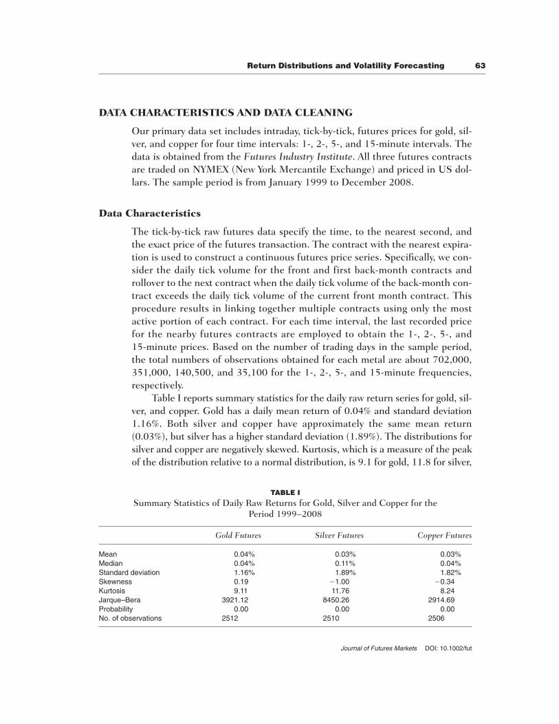
Table I reports summary statistics for the daily raw return series for gold, sil-ver, and copper. Gold has a daily mean return of 0.04% and standard deviation1.16%. Both silver and copper have approximately the same mean return(0.03%), but silver has a higher standard deviation (1.89%). The distributions forsilver and copper are negatively skewed. Kurtosis, which is a measure of the peakof the distribution relative to a normal distribution, is 9.1 for gold, 11.8 for silver,



TABLE I

Summary Statistics of Daily Raw Returns for Gold, Silver and Copper for the Period 1999–2008

Gold Futures Silver Futures Copper Futures

Mean 0.04% 0.03% 0.03%Median 0.04% 0.11% 0.04%Standard deviation 1.16% 1.89% 1.82%Skewness 0.19 �1.00 �0.34Kurtosis 9.11 11.76 8.24Jarque–Bera 3921.12 8450.26 2914.69Probability 0.00 0.00 0.00No. of observations 2512 2510 2506

and 8.24 for copper. The Jarque–Bera tests reject the null hypothesis that thesample raw returns for gold, silver, and copper come from a normal distribution.

Figure 1 shows the daily raw return series for gold, silver, and copper forthe period 1999–2008. All three return series exhibit a great deal of volatility,particularly after 2005, while showing a tendency for a constant mean. Acrossall three metals, the largest shocks to the return process took place towards theend of 2008 coinciding with the turmoil in financial markets. Also, in general,the volatility in silver and copper appear to be more pronounced than gold.

Figure 2 provides histograms of the raw return distribution for the threemetals. All three return distributions show that they are concentrated aroundthe mean, but exhibit fatter tails and sharper peaks at the mean of the returnsin comparison to the standard normal distribution. The negative skewnesscoefficient (i.e., a large probability of outcomes above the expected value) forsilver and copper are also visible from the graph. Once again, there is strongvisual evidence to suggest that the returns for gold, silver, and copper futuresdo not appear to be normally distributed.



1999 2000 2001 2002 2003 2004 2005 2006 2007 2008

�0.05

0

0.05

Daily raw return series for gold

1999 2000 2001 2002 2003 2004 2005 2006 2007 2008

�0.05

0

0.05

Daily raw return series for silver

1999 2000 2001 2002 2003 2004 2005 2006 2007 2008

�0.05

0

0.05

Daily raw return series for copper

FIGURE 1Daily raw returns for gold, silver, and copper for the period 1999–2008.

Figure 3 presents correlograms of the daily raw return series. Daily returnshave very little correlation which means that returns are almost impossible topredict from their own past history (up to 20 lags), and this is evidence that theunconditional mean is roughly constant.

Data Cleaning

Prior to conducting empirical analysis, a two-step procedure is employed to clean theraw data. First, in order to minimize bias in the results we eliminate days that haveinfrequent trades. During each normal trading day, the high-frequency data at five-minute interval should have about 72 price observations for gold, 70 observations forsilver, and 68 observations for copper. We remove those days from the samplewhere the number of five-minute price observations is less than 50% of the num-ber of price observations found in a normal trading day. For instance, there are 33days during which the gold contract had fewer than 36 five-minute price observations.



�0.1 �0.08 �0.06 �0.04 �0.02 0 0.02 0.04 0.06 0.08 0.1

200

400

Fre

quen

cy (

%)

Returns of gold during 1999–2008

Daily return series of gold

Daily returns of gold

Standard normal dist

�0.1 �0.08 �0.06 �0.04 �0.02 0 0.02 0.04 0.06 0.08 0.1

100

200

300

400

Fre

quen

cy (

%)

Returns of copper during 1999–2008

Daily return series of copper

Daily returns of copper


�0.1 �0.08 �0.06 �0.04 �0.02 0 0.02 0.04 0.06 0.08 0.1

200

400

Fre

quen

cy (

%)

Returns of silver during 1999–2008

Daily return series of silver

Daily returns of silver


FIGURE 2Histograms for gold, silver, and copper futures daily raw return series.

Similarly, the corresponding number of days with insufficient data for silver andcopper were 44 and 39, respectively. This resulted in a sample size of 2,480 days forgold, 2,467 days for silver, and 2,116 days for copper.2

Second, similar to Hansen and Lunde (2006) we eliminate days when theopening and closing transaction prices are the same. Zero daily returns are par-ticularly a problem when computing the loss functions associated with dailyabsolute returns. After removing those days from the sample, we end up withdata for 2,430, 2,375, and 2,061 days for gold, silver, and copper.

EMPIRICAL RESULTS

Comparing Volatility Measures

As a first step, we estimate integrated volatility using the four volatility meas-ures (see Equations (1), (3), (5), and (7)) and volatility estimated using the



0 2 4 6 8 10 12 14 16 18 20-0.5

0

0.5

1

Aut

ocor

rela

tion

Sample autocorrelation for copper

0 2 4 6 8 10 12 14 16 18 20-0.5

0

0.5

1

Aut

ocor

rela

tion

Sample autocorrelation for silver

0 2 4 6 8 10 12 14 16 18 20-0.5

0

0.5

1

20 lags(days)

Aut

ocor

rela

tion

Sample autocorrelation for gold

FIGURE 3Return correlograms for daily raw returns of gold, silver, and copper.

2We tried other filters that ranged from 30 to 60%, but the results were qualitatively similar. We thought thatthe 50% requirement was reasonable.

GARCH(1, 1) model. It is important to note that the GARCH model should notbe viewed as a benchmark, but just as another competing model that is used forcomparative purposes.

Table II summarizes the average annualized volatility, ofgold, silver, and copper for the cleaned data using different volatility measuresand different sampling frequencies. In the case of gold (see Panel A), for theone-minute interval, the estimated annual volatility is 16.74% using IVFT,13.92% using realized volatility measure, 13.33% using realized bipower volatil-ity, and 9.97% using daily absolute returns. The results indicate that the real-ized volatility measure is closest to the GARCH volatility estimate of 13.80%.Furthermore, the magnitudes of IVFT, realized volatility, and realized bipowervolatility decrease as the intraday time frequency decreases from 1-minute to15-minute interval.3

The corresponding results for silver and copper are shown in Panels B andC, respectively. These results are qualitatively similar to those of gold. Theabsolute return measure gives the lowest volatility estimates. Furthermore,across all different frequencies, IVFT is always greater than realized volatility,

2252 � sDaily,



3As pointed out earlier, the absolute return measure does not depend on the price movements during theperiod. Therefore, the same value is obtained for all time frequencies.

TABLE II

Annual Volatility Estimates of Gold, Silver and Copper for the Period 1999–2008

Time Frequency

Volatility Measure 1 minute 2 minutes 5 minutes 15 minutes

Panel A: Gold futures

GARCH daily (%) 13.80 13.80 13.80 13.80Daily absolute returns (%) 9.97 9.97 9.97 9.97Bipower variation (%) 13.33 12.67 12.03 10.96Realized volatility (%) 13.92 13.27 12.71 11.78IVFT (%) 16.74 14.52 13.77 11.98

Panel B: Silver futures

GARCH daily (%) 22.60 22.60 22.60 22.60Daily absolute returns (%) 16.51 16.51 16.51 16.51Bipower variation (%) 24.34 22.49 20.44 17.59Realized volatility (%) 25.69 23.86 21.94 19.43IVFT (%) 32.93 27.39 23.39 19.81

Panel C: Copper futures

GARCH daily (%) 19.31 19.31 19.31 19.31Daily absolute return (%)s 14.35 14.35 14.35 14.35Bipower Variation 19.84 18.63 17.57 15.92Realized volatility 20.59 19.44 18.42 17.01IVFT 26.44 22.14 20.60 18.47

and this in turn is greater than realized bipower volatility. This latter finding hasbeen highlighted by both Andersen et al. (2009) and Barndoff-Nielsen andShephard (2004). However, to the best of our knowledge, we are the first todocument that the magnitude of the IVFT estimate is the greatest among thefour volatility measures. This is perhaps because the IVFT measure is able toreflect more information about underlying price movements relative to othermeasures. Although it has been theoretically proven that both IVFT and bipow-er volatility measures are consistent estimators of integrated volatility, it isinteresting to note that the empirical estimates of the magnitude of the twovolatility measures are different from each other.

A couple of other interesting observations emerge. For the five-minuteinterval, the IVFT measure is the closest one to the GARCH (1,1) estimate.However, for the two-minute interval, the realized volatility estimates are veryclose to the GARCH (1, 1) results. We highlight the two- and five-minute fre-quencies, as these two frequencies are most commonly used in the literature toinvestigate intra-day volatility. An implication from these findings is that theIVFT measure or the realized volatility measure adds very little value relative tothe use of a simple GARCH (1, 1) model on daily data.

Daily Return Distributions

In this section, the distributional properties of daily speculative returns areinvestigated by using the Anderson et al. (2007) and Anderson et al. (2009)framework. For the sake of brevity, only the results pertaining to the five-minute interval is presented.

Table III presents the first four moments (m1 through m4) for the differentstandardized return series associated with the three markets, along with thecorresponding P-values for testing m1 � 0, m2 � 1, m3 � 0, and m4 � 3,respectively; except for the realized volatility standardized return series, forwhich the test for the fourth moment is based on the finite sample correction,

. Here, M is the number of observations during a regular tradingday. The results for gold, silver, and copper futures are reported in Panels A, B,and C in Table III. The QQ-plots for the corresponding distributions arereported in Figure 4.

Standardized return distributions

The first five rows in Table III report normality test results of returns standard-ized by unconditional volatility, GARCH(1, 1), and the three integrated volatili-ty measures—realized volatility, realized bipower volatility, and IVFT—usingfive-minute interval. It is clearly evident from the table that the different stan-dardized return series are not normally distributed.

m4 � 3 M

M � 2



TA

BL

E I

II

Nor

mal

ity

Test

Res

ults

for

Sta

ndar

dize

d R

etur

ns

m1

p 1m

2p 2

m3

p 3m

4p 4

p joi

ntp j

oint

-dm

Pane

l A: G

old

0.00

8245

0.68

1379

0.99

9665

0.99

0581

0.08

1351

0.29

5551

11.2

9416

00

00.

0260

250.

1950

60.

9994

090.

9834

070.

7440

51.

12E

�21

12.1

9727

00

00.

0336

120.

0941

570.

7023

351.

05E

�25

0.09

7625

0.20

9374

1.37

6437

1.56

E�

165.

12E

�24

1.2E

�23

0.04

3706

0.02

9514

0.92

5769

0.00

895

0.17

2006

0.02

6988

2.30

1483

0.00

0385

0.00

0829

0.00

4115

0.04

1057

0.04

0894

0.80

6709

1E�

110.

1394

950.

0728

681.

6883

22.

61E

�11

8.5E

�11

3.06

E�

100.

0568

180.

0046

620.

7447

552.

52E

�19

0.15

0154

0.05

3518

1.52

4087

6.31

E�

141.

87E

�18

3.34

E�

170.

0574

150.

0042

470.

7293

921.

59E

�21

0.14

8672

0.05

5921

1.49

5946

2.1E

�14

7.03

E�

211.

3E�

190.

0345

440.

0853

840.

8130

924.

65E

�11

0.07

7759

0.31

7387

1.90

0882

2.32

E�

081.

84E

�09

6.56

E�

090.

0772

420.

0853

840.

8579

530.

0252

890.

2757

380.

1128

322.

4213

130.

1883

840.

0463

620.

1220

06

Pane

l B: S

ilve

r

0.00

9597

0.63

3604

0.99

9687

0.99

1222

�0.

7621

21.

46E

�22

10.1

7161

2.2E

�28

90

00.

0172

400.

3919

326

1.00

0178

0.99

5001

�0.

4092

771.

542E

�07

9.16

865

1.41

E�

214

00

0.05

1616

0.01

0356

0.67

485

3.34

E�

300.

0930

810.

2325

921.

4713

849.

26E

�15

6.82

E�

339.

26E

�32

0.06

1098

0.00

2408

0.89

2035

0.00

015

0.13

2526

0.08

9212

2.54

773

0.02

1865

9.53

E�

060.

0004

750.

0561

710.

0052

720.

7407

868.

71E

�20

0.10

4399

0.18

0615

1.61

1917

1.97

E�

121.

02E

�19

3.05

E�

180.

0832

433.

56E

�05

0.69

1512

2.36

E�

270.

1721

760.

0272

41.

4524

694.

33E

�15

1.19

E�

308.

89E

�28

0.09

0475

7E–0

60.

6805

713.

3E�

290.

1480

790.

0575

61.

4299

121.

73E

�15

1.47

E�

347.

43E

�31

0.04

1897

0.03

7438

0.78

0056

1.12

E�

140.

0704

320.

3663

91.

7937

719.

67E

�10

1.2E

�13

8.97

E�

130.

0913

050.

0426

310.

8006

410.

0017

480.

2073

650.

2345

131.

8202

890.

0075

090.

0064

630.

0306

43R̂

* 5k,5

�25E

(CV

St)

R̂* k�2

E(C

VS

t)R̂

t�2

CV

St

R~ t�2

CV

t

Rt�2

RV

t

Rt�2

BV

t

Rt�2

IVF

Tt

Rt�2

GA

RC

H(1

,1)

Rt�2

Var

(Rt)

R̂* 5k

,5�2

5E(C

VS

t)R̂

* k�2

E(C

VS

t)R̂

t�2

CV

St

R~ t�2

CV

t

Rt�2

RV

t

Rt�2

BV

t

Rt�2

IVF

Tt

Rt�2

GA

RC

H(1

,1)

Rt�2

Var

(Rt)

(Con

tinu

ed)

TA

BL

E I

II (

Con

tinu

ed)

m1

p 1m

2p 2

m3

p 3m

4p 4

p joi

ntp j

oint

-dm

Pane

l C: C

oppe

r

0.07

9138

0.00

0272

1.00

579

0.85

061

0.52

3112

5.2E

�10

8.24

5035

6.9E

�13

40

00.

0798

150.

0002

420.

9973

890.

9323

240.

4598

774.

74E

�08

5.84

5674

1.08

E�

401.

8E�

161

5.2E

�15

10.

0806

290.

0002

080.

6932

041.

88E

�23

0.19

5206

0.02

0422

1.55

8982

1.33

E�

119.

46E

�27

1.15

E�

240.

1019

762.

72E

�06

0.94

0306

0.05

2177

0.35

2907

2.77

E�

052.

6283

680.

0810

272.

43E

�05

0.14

0342

0.09

3095

1.85

E�

050.

8345

527.

39E

�08

0.26

3809

0.00

1729

2.01

1543

3.47

E�

061.

27E

�09

1.55

E�

060.

0974

47.

39E

�06

0.76

6566

3.13

E�

140.

2437

920.

0037

851.

7815

611.

06E

�08

8.38

E�

171.

83E

�13

0.09

7409

7.44

E�

060.

7442

88.

96E

�17

0.21

8519

0.00

9448

1.67

3439

4.72

E�

101.

15E

�19

3.21

E�

160.

0784

910.

0003

050.

8781

347.

37E

�05

0.23

2824

0.00

5687

2.15

1055

6.73

E�

054.

95E

�06

0.00

0822

0.17

3917

0.00

0348

0.86

535

0.05

0204

0.51

4136

0.00

6329

2.23

6902

0.10

9194

0.00

2241

0.18

9111

Thi

s ta

ble

repo

rts

the

first

four

mom

ents

(m

1�

m4)

for

the

diffe

rent

sta

ndar

dize

d re

turn

ser

ies

for

the

thre

e m

arke

ts u

sing

5 m

inut

e in

terv

al, a

long

with

cor

resp

ondi

ng p

-val

ues

for

test

ing

m1

�0,

m2

�1,

m3

�0,

and

m4

�3,

res

pect

ivel

y, e

xcep

t for

the

real

ized

vol

atili

ty s

tand

ardi

zed

retu

rn s

erie

s, fo

r w

hich

the

test

for

the

four

th m

omen

t is

base

d on

the

finite

sam

ple

cor-

rect

ion,

.

Her

e, M

is t

he n

umbe

r of

obs

erva

tions

dur

ing

a re

gula

r da

y. T

he c

olum

n la

bele

d p j

oint

give

s th

e p-

valu

e fo

r te

stin

g th

e fo

ur m

omen

t co

nditi

ons

join

tly,

whi

le p

join

t–dm

refe

rs to

the

sam

e te

st in

volv

ing

the

(unc

ondi

tiona

lly)

dem

eane

d re

turn

ser

ies.

The

raw

dai

ly r

etur

ns a

re d

enot

ed b

y R

t, w

hile

an

d re

fer

to th

e da

ily ju

mp-

adju

sted

ret

urns

bas

ed o

nth

e si

mpl

e an

d se

quen

tial p

roce

dure

s, r

espe

ctiv

ely.

The

dai

ly r

ealiz

ed v

olat

ility

and

the

cor

resp

ondi

ng c

ontin

uous

com

pone

nt b

ased

on

the

sim

ple

and

sequ

entia

l jum

p-ad

just

ed p

roce

-du

res

are

deno

ted

by R

Vt,

CV

t, an

d C

VS

t, re

spec

tivel

y. V

ar(R

t) re

fers

to

the

unco

nditi

onal

var

ianc

e of

the

ret

urns

; G

AR

CH

(1,

1) is

the

con

ditio

nal v

aria

nce

estim

ated

by

a G

AR

CH

(1,

1)m

odel

; IV

FT

t, an

d B

Vtre

pres

ent

the

inte

grat

ed v

aria

nce

usin

g th

e F

ourie

r tr

ansm

issi

on a

ppro

ach

and

the

real

ized

bip

ower

vol

atili

ty w

ith 5

-min

ute

freq

uenc

y in

tra-

day

data

, re

spec

tivel

y.re

fers

to th

e fin

anci

al-t

ime

retu

rn s

erie

s co

nstr

uctin

g fr

om th

e se

quen

tial j

ump-

adju

sted

intr

aday

retu

rns

span

ning

E(C

VS

) tim

e-un

its. F

inal

ly,

defin

es th

e fin

anci

al-t

ime

retu

rn s

erie

s sp

anni

ng 5

E(C

VS

t) tim

e un

its.

R̂* 5k

,5�

R̂* 5k

�R̂

* 5k�

1�

R̂* 5k

�2

�R̂

* 5k�

3 �

R̂* 5k

�4

R̂* k

R̂t

R~ t

m4

�3

MM

�2

R̂* 5k

,5�2

5E(C

VS

t)R̂

* k�2

E(C

VS

t)R̂

* k�2

(CV

St)

R~ t�2

CV

t

Rt�2

RV

t

Rt�2

BV

t

Rt�2

IVF

Tt

Rt�2

GA

RC

H(1

,1)

Rt�2

Var

(Rt)

The unconditional returns and the GARCH(1, 1) standardized returnsremain significantly leptokurtic (very high fourth moment) for all three mar-kets. For instance, examining the unconditional returns in the gold market (seePanel A), the P-values of the first three-moment individual normality tests are0.68, 0.99, and 0.29. However, the P-value for the fourth moment normalitytest is zero. In comparison, the normality of the GARCH (1, 1) standardizedgold futures returns cannot be rejected only for the first two moments. Notably,the p-values of the first four-moment joint normality test is zero for both



Panel A: Gold futures

�4

�2

0

2

4

�4 �2 0 2 4

Quantiles of GC_BV

Qua

ntile

s of

Nor

mal

GC-BV

�4 �2 0 2 4

Quantiles of GC_FIN

Qua

ntile

s of

Nor

mal

GC-FIN

�3

�2

�1

0

1

2

3

�4 �2 0 2 4

Quantiles of GC_FIN5

Qua

ntile

s of

Nor

mal

GC-FIN5

�8 �4 0 4 8 12

Quantiles of GC_GARCH

Qua

ntile

s of

Nor

mal

GC-GARCH

�4

�2

0

2

4

�4

�2

0

2

4

�4

�2

0

2

4

�4 �2 0 2 4

Quantiles of GC_IVFT

Qua

ntile

s of

Nor

mal

GC-IVFT

�4

�2

0

2

4

�2�4 0 2 4

Quantiles of GC_RV

Qua

ntile

s of

Nor

mal

GC-RV

�4

�2

0

2

4

�4 �2 0 2 4

Quantiles of GC_SEJ

Qua

ntile

s of

Nor

mal

GC-SEJ

�4

�2

0

2

4

�4 �2 0 2 4

Quantiles of GC_SJ

Qua

ntile

s of

Nor

mal

GC-SJ

�4

�2

0

2

4

�10 �5 0 5 10

Quantiles of GC_VAR

Qua

ntile

s of

Nor

mal

GC-VAR

FIGURE 4. (Continued)

unconditional returns and GARCH (1, 1) standardized returns. One can arriveat a similar conclusion for silver and copper returns (see Panels B and C).

The normality of returns standardized by realized volatility, the realizedbipower volatility and the IVFT is rejected by the joint test at the 1% significantlevel. The realized bipower volatility does a better job than the other two meas-ures for all three markets. The p-values of the joint test for the bipower volatil-ity standardized returns are significantly higher than the other two measures.The IVFT measure does a better job in normalizing the third moment for allthree markets. The normality of IVFT standardized returns cannot be rejectedby the first and third moment individual tests at the 1% significant level for all



Panel B: Silver futures

�10 �5 0 5 10

Quantiles of SV_VAR

Qua

ntile

s of

Nor

mal

SV-VAR

�0.08

�0.04

0.00

0.04

0.08

�0 0.1 0.2 0.3 0.4

Quantiles of SV_GARCH

Qua

ntile

s of

Nor

mal

SV-GARCH

�4

�2

2

0

4

�6 �4 �2 0 2 4

Quantiles of SV_BV

Qua

ntile

s of

Nor

mal

SV-BV

�4

�2

0

2

4

�4 �2 0 2 4

Quantiles of SV_RV

Qua

ntile

s of

Nor

mal

SV-RV

�3

�2

�1

1

2

0

3

�4 �2 0 2 4

Quantiles of SV_IVFT

Qua

ntile

s of

Nor

mal

SV-IVFT

�4

�2

2

0

4

�4 �2 0 2 4

Quantiles of SV_SJ

Qua

ntile

s of

Nor

mal

SV-SJ

�4

�2

0

2

4

�4 �2 0 2 4

Quantiles of SV_SEJ

Qua

ntile

s of

Nor

mal

SV-SEJ

�3

�2

�1

1

2

0

3

�4 �2 0 2 4

�3

�2

�1

1

2

0

3

Quantiles of SV_FIN

Qua

ntile

s of

Nor

mal

SV-FIN

�4

�2

2

0

4

�4 �2 0 2 4

Quantiles of SV_FIN5

Qua

ntile

s of

Nor

mal

SV-FIN5

FIGURE 4. (Continued)

three markets. Interestingly, the IVFT measure seems to over-adjust the fourthmoment; in other words, IVFT-standardized daily returns show the lowestfourth moments across all three markets (1.376, 1.471, and 1.559 for gold, sil-ver, and copper, respectively).



Panel C: Copper futures

�4

�2

0

2

4

�8 �4 0 4 8

Quantiles of HG_VAR

Qua

ntile

s of

Nor

mal

HG-VAR

�4

�2

0

2

4

�8 �4 0 4 8

Quantiles of HG_GARCH

Qua

ntile

s of

Nor

mal

HG-GARCH

�4

�2

2

0

4

�4 �2 0 2 4

Quantiles of HG_RV

Qua

ntile

s of

Nor

mal

HG-RV

�4

�2

0

2

4

�10 �5 0 5 10

Quantiles of HG_BV

Qua

ntile

s of

Nor

mal

HG_BV

�3

�2

2

0

3

�4 �2 0 2 4

Quantiles of HG_IVFT

Qua

ntile

s of

Nor

mal

HG_IVFT

�4

�2

2

0

4

�6 �4 �2 0 2 4

Quantiles of HG_SJ

Qua

ntile

s of

Nor

mal

HG_SJ

�4

�2

0

2

4

�4 �2 0 2 4

Quantiles of HG_SEJ

Qua

ntile

s of

Nor

mal

HG-SEJ

�3

�2

�1

1

2

0

3

�4 �2 0 2 4

Quantiles of HG_FIN

Qua

ntile

s of

Nor

mal

HG-FIN

�4

�2

2

0

4

�4 �2 0 2 4

Quantiles of HG_FIN5

Qua

ntile

s of

Nor

mal

HG-FIN5

FIGURE 4QQ-plots of standardized returns of gold, silver and copper. The figure reports the QQ-plots of

standardized returns. GC, SV, and HG represent gold, silver and copper futures, respectively. **-VAR,**-GARCH, **-RV, **-BV, **-IVFT, **-SJ, **-SEJ, **-FIN, and **-FIN5 refer to the unconditionalreturns, returns standardized by GARCH(1, 1), realized volatility, realize bipower volatility, IVFT, the

continuous component of realized volatility based on the simple and sequential jump-adjustedprocedures, financial-time returns spanning E(CVSV) time-units standardized by E(CVSV), and

financial-time return series spanning 5E(CVSVt) time units standardized by 5E(CVSVt).

Standardized jump-adjusted returns

If there are no jumps and volatility leverage effects in the data, daily returnsshould be approximately normally distributed when standardized by integratedvolatilities. However, as indicated in the previous section, all the standardizedreturns are not normal, which implies that there might be some jumps in theintraday returns.

In an attempt to improve the normality of the return series, we apply simplejump adjustment and sequential jump adjustment procedures proposed byAndersen et al. (2009) to the five-minute intraday returns for the three markets.The basic idea behind the jump detection procedure is that the realized bipowervolatility measure is a consistent estimator of the integrated volatility even in thepresence of jumps, but the realized volatility is a consistent estimator of the inte-grated volatility only in the absence of jumps. Therefore, the difference betweenthose two measures identifies the jump component in realized volatility.

After identifying jumps, we remove the jump components from both dailyreturns and daily realized volatilities and arrive at daily jump-adjusted returns( and ) and continuous components of the realized volatility (CVt andCVSt). Subsequently, we standardize the daily jump-adjusted returns by thecorresponding continuous components of the daily realized volatilities. The 6thand 7th rows in Table III report the normality test results of the standardizeddaily jump-adjusted returns based on the simple and sequential jump identifi-cation procedures ( and ).

The results indicate that even after adjusting for jumps, we are unable toobtain normality to the standardized returns. Andersen et al. (2009) also reacha similar conclusion and attribute this finding to the self-standardizing natureof jumps. The authors indicate that, “a large jump tends to inflate the absolutevalue of both the return and the realized volatility of standardized returns, sothe impact is muted.” Therefore, we extend the analysis to evaluate the proper-ties of jump-adjusted standardized returns sampled in financial-time in the nextsection.

Standardized jump-adjusted financial-time returns

To sample in financial-time, or equal increments of integrated volatility, weinclude intraday returns until the cumulative squared returns exceeds the aver-age continuous component of daily realized volatility in calendar time for thesequential jump-adjusted returns. That is, we only include the non-jumpreturns identified by the sequential jump detection procedure. For the purposeof comparing our results derived from financial-time with previous results, wecalibrate the number of financial days to equal the number of calendar days inthe sample. We consider one financial day if the cumulative squared returns

R� t�2CVStR~

t�2CVt

R� tR~

t



exceed the average continuous components of the daily realized volatility, or ifthe difference between the two values is less than a small value. We samplerepeatedly by adjusting the magnitude of the small value until the number offinancial days equals the number of calendar days.

The last two rows in Table III report the normality tests of the financial-time return series constructed from: (a) sequential jump-adjusted intradayreturns spanning E(CVSt), which is the average continuous component of thesequential jump-adjusted realized volatility; and (b) 5E(CVSt) time units.Evidence from all three markets indicates that the standardized daily financial-time returns are still not normal based on the joint test of the four moments.However, normality in the return distribution is restored for all three marketswhen considering the demeaned financial-time returns series spanning5E(CVSt) time units. In this case, normality cannot be rejected at the 1% level.

The QQ-plots in Figure 4 (Panels A, B, and C) show that in comparison tounconditional returns and GARCH (1, 1) standardized return distributions, theremaining standardized distributions are much closer to the referenceGaussian distribution. Notably, tails of the QQ-plots show significant improve-ment and display only slight deviations from the straight 45° line.

Comparing our results with Andersen et al.’s (2009) evidence on stockreturns, we find that the normality for metal futures returns is somewhat moredifficult to establish. Andersen et al. (2009) succeed in restoring normality for24 out of the 30 stocks in the Dow Jones Industrial Average at the 1% signifi-cance level using financial time returns. However, in our study we reject normality of the standardized financial day returns at the 1% level of signifi-cance. To be sure we tried different sampling frequencies, but the results werequalitatively similar. We conjecture that this difficulty in establishing normalityfor metal futures returns might be attributable to some additional microstruc-ture noise that may be prevalent in these markets.

In conclusion, the unconditional returns of futures prices are not normallydistributed. When we standardize returns with IVFT and realized volatility meas-ures, the corresponding return distributions bear closer resemblance to a normaldistribution. By applying the newly developed financial-time sampling techniqueproposed by Andersen et al. (2009), we succeed in converting the return seriesinto i.i.d. Gaussian for all three markets. The added difficulties of restoring nor-mality for futures returns are a topic that may require further investigation.

Forecast Performance of GARCH(1, 1) Model UsingDifferent Volatility Measures as Volatility Proxies

In the concluding step of the analysis, the predictive performance of theGARCH(1, 1) forecasting model is evaluated using the four different volatility



measures. As suggested by Patton (2009), forecasting accuracy is compared byusing the QLIKE loss function, although we report the values for all five differ-ent loss functions.

For the purpose of comparing our results with evidence from prior litera-ture, we first value from traditional loss functions such as HRMSE and LL.4

The results indicate that both HRMSE and LL functions strongly documentthe GARCH model using the IVFT estimator which produces volatility fore-casts that are more accurate when compared with other measures. The evi-dence provides support for Nielsen and Frederiksen (2008) and Reno andBarucci (2002) who posit that the IVFT measure is a better measure of inte-grated volatility than realized volatility. Also consistent with Anderson andBollerslev (1998a) and others, the results using HRMSE and LL loss functionsindicate that forecasting performance of the GARCH(1, 1) model improves asthe time frequency increases from 15- to 1-minute intervals.

Table IV reports the values associated with the new family of loss func-tions using the 1-, 2-, 5-, and 15-minute time intervals for gold, silver, and cop-per. Several important insights are documented. First, forecasting performanceof the GARCH (1, 1) model depends on both the volatility proxy and intradaytime frequency that is used in the analysis. For the 5- and 15-minute frequen-cies, the GARCH (1, 1) model has the smallest forecast errors (i.e., least lossfunction values) when the IVFT measure. This is true for all three metals.However, if we increase the time frequency to two or one $$minute, the lowestforecasting error is obtained when the realized volatility proxy is used. The sil-ver market provides the only exception to this finding; here the two-minuteinterval using IVFT produces the smallest forecasting error.

Second, unlike the results from HRMSE and LL, increasing the time fre-quency in general does not necessarily improve the predictive performance ofthe GARCH (1, 1) model. For instance, when IVFT is used, only the five-minute interval provides the lowest forecasting error. In the case of realizedvolatility, however, forecast performance improves with the intraday time fre-quency used to measure daily returns. It may be worth pointing out that theseconclusions are broadly consistent with the results in Table II, which docu-ments that the realized volatility estimate gets closer to the GARCH (1, 1)volatility estimate as the intraday frequency used to measure daily returnsincreases.

Third, and not surprisingly, the GARCH (1, 1) forecasting model yields thelargest forecast error when using the daily absolute return measure. This isbecause by definition the daily absolute return measure does not integrateintraday information into the estimation procedure.



4These results are not reported but can be made available by the authors upon request.

TABLE IV

Forecast Performance of the GARCH (1, 1) Model

Value of Loss Functions

Time Volatility b

Frequency Market Measure �5 �2 �1 0 1

1 Minute Gold D–ABS 3.39E�27 152328 0.314419 7.99E�05 1.84E�07IVFT 2.11E�15 473.3238 0.074112 2.56E�05 1.76E�08BV 3.71E�17 502.3164 0.037622 9.18E�06 5.89E�09RV 1.74E�17 429.6906 0.03828 1.06E�05 7.05E�09

Silver D–ABS 3.12E�24 72652.34 0.77424 0.000495 2.96E�06IVFT 1.01E�14 881.3926 0.368876 0.000268 4.24E�07BV 5.13E�16 428.1604 0.106149 7.81E�05 1.27E�07RV 1.37E�16 391.9233 0.119774 0.000113 2.68E�07

Copper D–ABS 1.16E�14 5725.963 17.11383 0.158213 0.003068IVFT 9.67E�13 491.7552 0.144392 7.8E�05 8.55E�08BV 3.95E�14 236.1186 0.04753 2.29E�05 2.41E�08RV 1.3E�14 202.5782 0.047681 2.56E�05 2.72E�08

2 Minutes Gold D–ABS 3.39E�27 152328 0.314419 7.99E�05 1.84E�07IVFT 1.02E�16 415.0369 0.047485 1.51E�05 1.06E�08BV 1.64E�18 742.5116 0.046472 1.21E�05 1.05E�08RV 5.28E�17 599.7234 0.044266 1.19E�05 8.88E�09

Silver D–ABS 3.12E�24 72652.34 0.77424 0.000495 2.96E�06IVFT 1.5E�14 539.111 0.16905 0.000107 1.59E�07BV 7.17E�16 484.5708 0.102449 6.72E�05 9.86E�08RV 2.16E�16 397.294 0.107412 8.53E�05 1.51E�07



Silver D–ABS 3.12E�24 72652.34 0.77424 0.000495 2.96E�06IVFT 5.2E�14 384.3816 0.113635 8.56E�05 1.39E�07BV 1.03E�17 815.1069 0.126349 6.36E�05 8.65E�08RV 8.47E�16 617.2162 0.125764 8.45E�05 1.35E�07



Silver D–ABS 3.12E�24 72652.34 0.77424 0.000495 2.96E�06IVFT 3.8E�17 1270.958 0.169335 9.67E�05 1.98E�07BV 1.62E�27 8863.144 0.199 5.73E�05 5.25E�08RV 9.89E�17 1509.009 0.177228 9.78E�05 2.18E�07


This table reports the values of the loss functions of the one day ahead forecasting of the GARCH (1,1) model using different volatil-ity measures as volatility proxies. In the table, D–ABS refers to the daily absolute returns measure; IVFT and BV represent the inte-grated volatility using the Fourier transmission approach and the realized bipower volatility; RV refers to the realized volatility.

Finally, a comparison of different volatility forecasts indicates that copperhas the lowest forecast error, followed by silver and gold. Although this findingcannot be explained within the context of the study, one might surmise that thisresult is being partly driven by the price discovery and volatility transmissionprocess among strategically linked metals market (see Adrangi, Chatrath, &David, 2000).

CONCLUSIONS

A large amount of literature has been devoted to estimating and forecastingvolatility for financial time series. In this field, the importance of high-frequencydata has been stressed, in particular for evaluating the predictive abilities ofvolatility models. This study uses intraday futures prices for gold, silver, andcopper for the period 1998–2009 to examine the return distribution propertiesand estimate four integrated measures of volatility—absolute returns, realizedvolatility, realized bipower volatility, and IVFT.

The study finds that the daily futures returns are generally not normal, evenwhen standardized by various integrated volatility measures. However, restora-tion of normality is possible by applying the recently developed sequential jumpdetection scheme and financial-time sampling techniques. It is interesting tonote that establishing a normal distribution for the metal futures market isfound to be more difficult than that for the stock market, an issue that is leftfor future investigation.

The study further documents that, in general, IVFT and realized volatilityare relatively efficient proxies of volatility in the metal futures market. The IVFTmeasure is always greater than realized volatility followed by realized bipowervolatility for all different frequencies—an indication that the IVFT measuremay reflect more information about underlying price movements than othervolatility measures.

Finally, the forecast accuracy of the GARCH (1, 1) model is assessed byusing a set of robust loss functions. The results indicate that for the two- andfive-minute time frequencies, which are most commonly used in the literature,both realized volatility and IVFT measures provide low forecasting errors.Notably, an increase in the time frequency does not necessarily improve theforecasting performance of the GARCH (1, 1) model.

The research highlights the importance of integrated volatility measuresand high-frequency sampling techniques in analyzing the distributional proper-ties of futures returns. In particular, gauging the usefulness of volatility forecasts requires a refined articulation of volatility, as well as construction ofintegrated volatility measures that captures the concept in an empirically robust



fashion. Finally, an evaluation of competing forecasting models is partlydependent on the specific loss function that is used.

There are many possible ways to extend this study. For instance, it wouldbe interesting to examine the response of price movements to new informationor “news,” and investigate the connections between the identified jump compo-nents with news arrival. An analysis of jumps across markets, or co-jumps,along with volatility transmission would also be a worthwhile endeavor. Thesetopics are left for future research.

BIBLIOGRAPHY

Adrangi, B., Chatrath, A., & David, C. (2000). Price discovery in strategically-linkedmarkets: The case of the gold-silver spread. Applied Financial Economics, 10,227–234.

Aggarwal, R., & Soenen, L. A. (1991). The nature and efficiency of the gold market.The Journal of Portfolio Management, 14, 18–21.

Akgiray, V., Booth, G., Hatem, J., & Chowdary, M. (1991). Conditional dependence inprecious metal prices. The Financial Review, 26, 367–386.

Andersen, T., & Bollerslev, T. (1998a). DM-Dollar intraday volatility: Activity pattern,macroeconomic announcemnets, and longer run dependences. Journal ofFinance, 53, 219–265.

Andersen, T., & Bollerslev, T. (1998b). Answering the skeptics. International EconomicReview, 39, 885–905.

Andersen, T., Bollerslev, T., & Diebold, F. (2005). Parametric and nonparametricvolatility measurement. In Y. Aot-Sahalia, & L. Hansen (Ed.), Handbook of finan-cial econometrics (pp. 67–138). Amsterdam: North-Holland.

Andersen, T., Bollerslev, T., & Dobrev, D. (2007). No-Arbitrage semi-martingle restric-tions for continous-time volatility models subject to leverage effects, jumps and i.i.d.noise: Theory and testable distributional implications. Journal of Econometrics,138, 125–180.

Andersen, T., Bollerslev, T., Frederiksen, P., & Nielsen, M. Ø. (2010). Continuous-timemodels, realized volatilities, and testable distributional implications for daily stockreturns. Journal of Applied Econometrics; Forthcoming, 25, 233–261.

Andersen, T., Bollerslev, T., & Lange, S. (1999). Forecasting financial market volatility.Journal of Empirical Finance, 6, 457–477.

Andersen, T., Diebold, F., Labys, P., & Bollerslev, T. (2001). Modeling and forecastingrealized volatility (NBER Working Paper, No. 8160) Econometrica, 71, 579–625.

Baillie, R., & Bollerslev, T. (1992). Prediction in dynamic models with time-dependentconditional variances. Journal of Econometrics, 52, 91–113.

Barndoff-Nielsen, O. E., & Shepard, N. (2001). Non-Gaussian OU based models andsome of their uses in financial economics. Journal of the Royal Statistical Society,Series B 63, 167–241.

Barndoff-Nielsen, O. E., & Shephard, N. (2004). Power and bipower variation withstochastic volatility and jumps. Journal of Financial Econometrics, 2, 1–48.

Ciner, C. (2001). On the long run relationship between gold and silver rrices: A note.Global Finance Journal, 12, 299–303.



Cumby, R., Figlewski, S., & Hasbrouk, J. (1993). Forecasting volatility and autocorre-lation in the EGARCH models. Journal of Derivative, 1, 51–75.

Figlewski, S. (1997). Volatility forecasting. Journal of Financial Markets, Institutionsand Instruments, 6, 1–88.

Hansen, P. R., & Lunde, A. (2005). A realized variance for the whole day based onintermittent high-frequency data. Journal of Financial Econometrics, 3, 525–554.

Hansen, P. R., & Lunde, A. (2006). Realized variance and market microstructure noise.Journal of Business and Economic Statistics, 24, 127–161.

Kocagil, A. (1997). Does futures speculation stabilize spot prices? Evidence from metalmarkets. Applied Financial Economics, 7, 113–125.

Koopman, S. J., Jungbacker, B., & Hol, E. (2005). Forecasting daily variability of theS&P100 stock index using historical, realised and implied volatility measurement.Journal of Empirical Finance, 12, 445–475.

Krehbiel, T., & Adkins, L. C. (1993). Cointegration tests of the unbiased expectationhypothesis in metals markets. The Journal of Futures Markets, 13, 753–763.

Lucey, B., & Tully, E. (2006). Seasonality, risk and return in daily COMEX gold and sil-ver data 1982–2002. Applied Financial Economics, 16, 48–59.

Malliavin, P., & Mancino, M. E. (2002). Fourier series method for measurement ofmultivariate volatility. Finance and Stochastics, 6, 49–61.

Mancino, M. E., & Sanfelici, S. (2009). Robustness of Fourier estimator of integratedvolatility in the presence of microstrucuture noise. Computational Statisitics &Data Analysis, 51, 2966–2989.

Nielsen, M., & Frederiksen, P. (2008). Finite sample accuracy and choice of samplingfrequency in integrated volatility estimation. Journal of Empirical Finance, 15,265–286.

Patton, A. (2009). Volatility forecast comparison using imperfect volatility proxies.Journal of Econometrics; Forthcoming.

Poon, S., & Granger, C. (2003). Forecasting volatility in financial markets: A review.Journal of Economic Literature, 41, 478–539.

Reno, R., & Barucci, E. (2002). On measuring volatility and the GARCH forecastingperformance. Journal of International Financial Markets, Institutions and Money,12, 183–200.

West, K., & Cho, D. (1995). The predictive ability of several models of exchange ratevolatility. Journal of Econometrics, 69, 367–391.



Return distributions and volatility forecasting in metal ...

Documents

Transcript of Return distributions and volatility forecasting in metal ...