Volatility indices, volatility forecasting, Granger causality.

FUNDAÇÃO GETULIO VARGAS
SÃO PAULO SCHOOL OF ECONOMICS
THIAGO WINKLER ALVES
FORECASTING DAILY VOLATILITY USING HIGHFREQUENCY FINANCIAL DATA
SÃO PAULO
2014

THIAGO WINKLER ALVES
FORECASTING DAILY VOLATILITY USING HIGHFREQUENCY FINANCIAL DATA
Dissertation presented to the ProfessionalMaster Program from the São Paulo School ofEconomics, part of Fundação Getulio Vargas,in partial fulfillment of the requirements forthe degree of Master of Economics, with amajor in Quantitative Finance.
Supervisor:Prof. Dr. Juan Carlos Ruilova Terán
SÃO PAULO2014

Winkler Alves, Thiago.Forecasting Daily Volatility Using High Frequency Financial Data / Thiago
Winkler Alves – 2014.77 f.
Orientador: Prof. Dr. Juan Carlos Ruilova Terán.Dissertação (MPFE) – Escola de Economia de São Paulo.
1. Mercado financeiro - Modelos econométricos. 2. Análise de séries temporais.3. Mercado futuro. I. Ruilova Terán, Juan Carlos. II. Dissertação (MPFE) – Escolade Economia de São Paulo. III. Título.
CDU 336
THIAGO WINKLER ALVES
FORECASTING DAILY VOLATILITY USING HIGHFREQUENCY FINANCIAL DATA
Dissertation presented to the ProfessionalMaster Program from the São Paulo School ofEconomics, part of Fundação Getulio Vargas,in partial fulfillment of the requirements forthe degree of Master of Economics, with amajor in Quantitative Finance.
Date of Approval: August 6th, 2014
Examining Committee:
Prof. Dr. Juan Carlos Ruilova Terán(Supervisor)
Fundação Getulio Vargas
Prof. Dr. Alessandro Martim MarquesFundação Getulio Vargas
Prof. Dr. Hellinton Hatsuo TakadaInsper

To my parents, Jaqueline and Ary,and to my little sister, Marina.

ACKNOWLEDGEMENTS
To my grandmothers and parents, who taught me and my sister how importantstudying is. She, even six years younger, keeps inspiring me with her daily conquests.
To Vicki, because revising the English in my writing was the smallest contributionshe ever made me. Thank you for all the support, even when it meant I would be away.
To all my Professors, but especially to Prof. Dr. Juan Carlos Ruilova Terán andProf. Dr. Alessandro Martim Marques, for all the knowledge and precious advice given.
To all my friends and colleagues, particularly to Wilson Freitas and Thársis Souza,who are always available to sit at a bar table and talk finance while drinking beer.
Finally, it is also important to thank Itaú Unibanco for the financial support.Without it, this degree would not be possible.

“Wahrlich es ist nicht das Wissen, sondern das Lernen,nicht das Besitzen, sondern das Erwerben,
nicht das Da-Seyn, sondern das Hinkommen,was den größten Genuss gewährt.”
(Johann Carl Friedrich Gauß)

ABSTRACTAiming at empirical findings, this work focuses on applying the HEAVY model for dailyvolatility with financial data from the Brazilian market. Quite similar to GARCH, thismodel seeks to harness high frequency data in order to achieve its objectives. Four variationsof it were then implemented and their fit compared to GARCH equivalents, using metricspresent in the literature. Results suggest that, in such a market, HEAVY does seem tospecify daily volatility better, but not necessarily produces better predictions for it, whatis, normally, the ultimate goal.
The dataset used in this work consists of intraday trades of U.S. Dollar and Ibovespafuture contracts from BM&FBovespa.
Keywords: financial engineering. volatility forecast. high frequency financial data. futuresmarket.

RESUMOObjetivando resultados empíricos, este trabalho tem foco na aplicação do modelo HEAVYpara volatilidade diária com dados financeiros do mercado Brasileiro. Muito similarao GARCH, este modelo busca explorar dados em alta frequência para atingir seusobjetivos. Quatro variações dele foram então implementadas e seus ajustes comparadadosa equivalentes GARCH, utilizando métricas presentes na literatura. Os resultados sugeremque, neste mercado, o HEAVY realmente parece especificar melhor a volatilidade diária,mas não necessariamente produz melhores previsões, o que, normalmente, é o objetivofinal.
A base de dados utilizada neste trabalho consite de negociações intradiárias de contratosfuturos de dólares americanos e Ibovespa da BM&FBovespa.
Palavras-chave: engenharia financeira. previsão de volatilidade. dados financeiros emalta frequência. mercado de futuros.

List of Figures
Figure 1 – Weak-sense stationarity example . . . . . . . . . . . . . . . . . . . . . 20Figure 2 – Random walk example . . . . . . . . . . . . . . . . . . . . . . . . . . . 22Figure 3 – HEAVY (in black) vs GARCH (in gray) adjustment to volatility changes 42
List of Tables
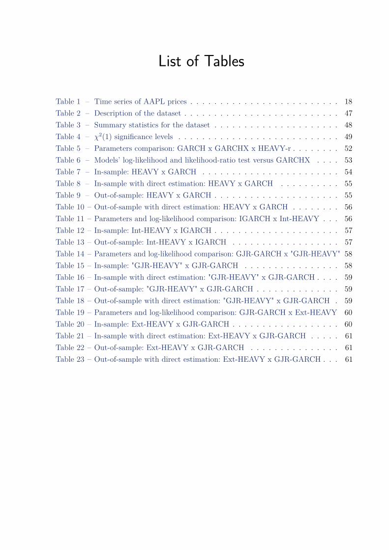
Table 1 – Time series of AAPL prices . . . . . . . . . . . . . . . . . . . . . . . . . 18Table 2 – Description of the dataset . . . . . . . . . . . . . . . . . . . . . . . . . . 47Table 3 – Summary statistics for the dataset . . . . . . . . . . . . . . . . . . . . . 48Table 4 – χ2(1) significance levels . . . . . . . . . . . . . . . . . . . . . . . . . . . 49Table 5 – Parameters comparison: GARCH x GARCHX x HEAVY-r . . . . . . . . 52Table 6 – Models’ log-likelihood and likelihood-ratio test versus GARCHX . . . . 53Table 7 – In-sample: HEAVY x GARCH . . . . . . . . . . . . . . . . . . . . . . . 54Table 8 – In-sample with direct estimation: HEAVY x GARCH . . . . . . . . . . 55Table 9 – Out-of-sample: HEAVY x GARCH . . . . . . . . . . . . . . . . . . . . . 55Table 10 – Out-of-sample with direct estimation: HEAVY x GARCH . . . . . . . . 56Table 11 – Parameters and log-likelihood comparison: IGARCH x Int-HEAVY . . . 56Table 12 – In-sample: Int-HEAVY x IGARCH . . . . . . . . . . . . . . . . . . . . . 57Table 13 – Out-of-sample: Int-HEAVY x IGARCH . . . . . . . . . . . . . . . . . . 57Table 14 – Parameters and log-likelihood comparison: GJR-GARCH x "GJR-HEAVY" 58Table 15 – In-sample: "GJR-HEAVY" x GJR-GARCH . . . . . . . . . . . . . . . . 58Table 16 – In-sample with direct estimation: "GJR-HEAVY" x GJR-GARCH . . . . 59Table 17 – Out-of-sample: "GJR-HEAVY" x GJR-GARCH . . . . . . . . . . . . . . 59Table 18 – Out-of-sample with direct estimation: "GJR-HEAVY" x GJR-GARCH . 59Table 19 – Parameters and log-likelihood comparison: GJR-GARCH x Ext-HEAVY 60Table 20 – In-sample: Ext-HEAVY x GJR-GARCH . . . . . . . . . . . . . . . . . . 60Table 21 – In-sample with direct estimation: Ext-HEAVY x GJR-GARCH . . . . . 61Table 22 – Out-of-sample: Ext-HEAVY x GJR-GARCH . . . . . . . . . . . . . . . 61Table 23 – Out-of-sample with direct estimation: Ext-HEAVY x GJR-GARCH . . . 61

List of abbreviations and acronyms
AR AutoRegressive
ARCH AutoRegressive Conditional Heteroskedasticity
ARIMA AutoRegressive Integrated Moving Average
ARIMAX ARIMA with Explanatory Variables
ARMA AutoRegressive Moving Average
DOL BM&FBovespa’s U.S. Dollar Future Contract
EWMA Exponentially Weighted Moving Average
Ext-HEAVY Extended High-frEquency-bAsed VolatilitY
GARCH Generalized AutoRegressive Conditional Heteroskedasticity
GARCHX GARCH with Explanatory Variables
GJR-GARCH Glosten-Jagannathan-Runkle-GARCH
HEAVY High-frEquency-bAsed VolatilitY
HFT High Frequency Trading
IGARCH Integrated Generalized AutoRegressive Conditional Heteroskedasticity
IND BM&FBovespa’s Ibovespa Future Contract
Int-HEAVY Integrated High-frEquency-bAsed VolatilitY
MA Moving Average
MLE Maximum-Likelihood Estimation
MSRV MultiScale Realized Variance
OLS Ordinary Least Squares
PDF Probability Density Function
RM Realized Measure
RS Realized Semivariance
RV Realized Variance
WSS Weak-Sense Stationary
Contents
Introduction 14Objectives . . . . . . . . . . . . . . . . . . . . . . . . . . . . . . . . . . . . . . . 15Organization . . . . . . . . . . . . . . . . . . . . . . . . . . . . . . . . . . . . . 16
I Financial Series Modeling 17
1 General Definitions . . . . . . . . . . . . . . . . . . . . . . . . . . . . . . . . 181.1 Time Series . . . . . . . . . . . . . . . . . . . . . . . . . . . . . . . . . . . 181.2 Stationarity . . . . . . . . . . . . . . . . . . . . . . . . . . . . . . . . . . . 191.3 Linear Regression . . . . . . . . . . . . . . . . . . . . . . . . . . . . . . . . 201.4 High Frequency Financial Data . . . . . . . . . . . . . . . . . . . . . . . . 21
2 Mean Models . . . . . . . . . . . . . . . . . . . . . . . . . . . . . . . . . . . 222.1 Random Walk . . . . . . . . . . . . . . . . . . . . . . . . . . . . . . . . . . 222.2 Autoregressive Models . . . . . . . . . . . . . . . . . . . . . . . . . . . . . 23
2.2.1 Forecasting . . . . . . . . . . . . . . . . . . . . . . . . . . . . . . . 242.3 Moving Average Models . . . . . . . . . . . . . . . . . . . . . . . . . . . . 252.4 Autoregressive Moving Average Models . . . . . . . . . . . . . . . . . . . . 252.5 Autoregressive Integrated Moving Average Models . . . . . . . . . . . . . . 262.6 ARIMA with Explanatory Variables Models . . . . . . . . . . . . . . . . . 26
3 Estimation . . . . . . . . . . . . . . . . . . . . . . . . . . . . . . . . . . . . . 273.1 Ordinary Least Squares . . . . . . . . . . . . . . . . . . . . . . . . . . . . . 273.2 Maximum-Likelihood . . . . . . . . . . . . . . . . . . . . . . . . . . . . . . 29
II Volatility Models 31
4 GARCH Family . . . . . . . . . . . . . . . . . . . . . . . . . . . . . . . . . . 324.1 ARCH . . . . . . . . . . . . . . . . . . . . . . . . . . . . . . . . . . . . . . 324.2 GARCH . . . . . . . . . . . . . . . . . . . . . . . . . . . . . . . . . . . . . 33
4.2.1 Estimating . . . . . . . . . . . . . . . . . . . . . . . . . . . . . . . . 344.2.2 Forecasting . . . . . . . . . . . . . . . . . . . . . . . . . . . . . . . 35
4.3 IGARCH . . . . . . . . . . . . . . . . . . . . . . . . . . . . . . . . . . . . . 354.4 GARCH with Explanatory Variables . . . . . . . . . . . . . . . . . . . . . 364.5 GJR-GARCH . . . . . . . . . . . . . . . . . . . . . . . . . . . . . . . . . . 36

5 Realized Measures . . . . . . . . . . . . . . . . . . . . . . . . . . . . . . . . 375.1 Realized Variance . . . . . . . . . . . . . . . . . . . . . . . . . . . . . . . . 375.2 Multiscale Realized Variance . . . . . . . . . . . . . . . . . . . . . . . . . . 385.3 "Realized EWMA" . . . . . . . . . . . . . . . . . . . . . . . . . . . . . . . 395.4 Subsampling . . . . . . . . . . . . . . . . . . . . . . . . . . . . . . . . . . . 405.5 Realized Semivariance . . . . . . . . . . . . . . . . . . . . . . . . . . . . . 40
6 HEAVY Family . . . . . . . . . . . . . . . . . . . . . . . . . . . . . . . . . . 416.1 HEAVY . . . . . . . . . . . . . . . . . . . . . . . . . . . . . . . . . . . . . 41
6.1.1 Estimating . . . . . . . . . . . . . . . . . . . . . . . . . . . . . . . . 436.1.2 Forecasting . . . . . . . . . . . . . . . . . . . . . . . . . . . . . . . 44
6.2 Int-HEAVY . . . . . . . . . . . . . . . . . . . . . . . . . . . . . . . . . . . 456.3 "GJR-HEAVY" . . . . . . . . . . . . . . . . . . . . . . . . . . . . . . . . . 456.4 Extended HEAVY . . . . . . . . . . . . . . . . . . . . . . . . . . . . . . . 45
III Application 46
7 Dataset Description . . . . . . . . . . . . . . . . . . . . . . . . . . . . . . . 47
8 Evaluation Metrics . . . . . . . . . . . . . . . . . . . . . . . . . . . . . . . . 498.1 Likelihood-ratio Test . . . . . . . . . . . . . . . . . . . . . . . . . . . . . . 498.2 Loss Function . . . . . . . . . . . . . . . . . . . . . . . . . . . . . . . . . . 508.3 Direct Estimation and Forecasting . . . . . . . . . . . . . . . . . . . . . . . 51
9 Experiments and Results . . . . . . . . . . . . . . . . . . . . . . . . . . . . . 529.1 Realized Measures versus Squared Returns . . . . . . . . . . . . . . . . . . 529.2 HEAVY versus GARCH . . . . . . . . . . . . . . . . . . . . . . . . . . . . 549.3 Int-HEAVY versus IGARCH . . . . . . . . . . . . . . . . . . . . . . . . . . 569.4 "GJR-HEAVY" versus GJR-GARCH . . . . . . . . . . . . . . . . . . . . . 579.5 Ext-HEAVY versus GJR-GARCH . . . . . . . . . . . . . . . . . . . . . . . 60
Conclusion 62Future Directions . . . . . . . . . . . . . . . . . . . . . . . . . . . . . . . . . . . 62Further Comments . . . . . . . . . . . . . . . . . . . . . . . . . . . . . . . . . . 63
Bibliography . . . . . . . . . . . . . . . . . . . . . . . . . . . . . . . . . . . . . 64
Appendix 66
APPENDIX A Database Construction . . . . . . . . . . . . . . . . . . . . . . 67
Annex 69
ANNEX A Code Listings . . . . . . . . . . . . . . . . . . . . . . . . . . . . . . 70
14
Introduction
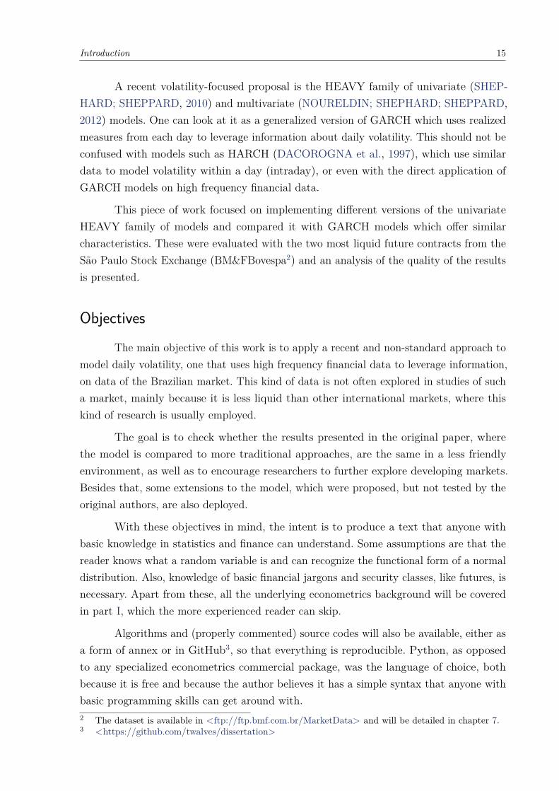
Early exchange houses (bourses) first appeared in the XIII century, and evolved intowhat we now know as the securities exchange market. Advances in computer technologyin the last decades have taken these central pieces of world economy from places whereone could find yelling traders to complex electronic trading systems. Evolution then wasnatural: investors want their orders to be executed before prices change; and the moretrades happen during a day, the more bourses earn with fees. The competition betweenexchanges also raises the pace of such technological evolution, and an ever decreasinglatency time became the objective of most of them.
Automated and algorithmic trading systems take a big role in today’s globaleconomy. This move from manual trades allows investors to grow and diversify theirportfolios more easily, and with faster and cheaper technology available, even more marketagents will follow this trend. The necessary speed for making decisions requires accuratemethods, justifying the study of high frequency trading (HFT) techniques and their effects.
The study of this new environment, created by financial markets that operate at amuch higher speed, and are much more interconnected, is in the edge of research in finance1.It is also of great importance, not only because of all the capacity it has for generatingprofit, but mainly because of the understanding it can provide of the microstructure ofthe market, allowing both regulators and market players to keep it healthy and profitable(SCHMIDT, 2011).
Along with these technological advances, the amount of data that becomes availableto researchers and market players significantly increases and econometric models that tryto harness all this new information also emerge. Most of these models seek to uncover thedynamics of the prices of assets, and less attention is given to volatility models.
Different from prices, volatility is not observable, really difficult to precisely measure,and, as a consequence, not easy to model. But being able to do so is of great value, becauseit has direct application in things such as trading strategies and, more importantly, riskmanagement.
When dealing only with daily information to model volatility, the first majorrecognized family - a family, because the number of parameters may vary - of modelsis ARCH (ENGLE, 1982), followed four years later by GARCH (BOLLERSLEV, 1986),which, along with its variations, is up to this day the most known and used family of dailyvolatility models.1 <http://kolmogorov.math.stevens.edu/conference2013>
Introduction 15
A recent volatility-focused proposal is the HEAVY family of univariate (SHEP-HARD; SHEPPARD, 2010) and multivariate (NOURELDIN; SHEPHARD; SHEPPARD,2012) models. One can look at it as a generalized version of GARCH which uses realizedmeasures from each day to leverage information about daily volatility. This should not beconfused with models such as HARCH (DACOROGNA et al., 1997), which use similardata to model volatility within a day (intraday), or even with the direct application ofGARCH models on high frequency financial data.
This piece of work focused on implementing different versions of the univariateHEAVY family of models and compared it with GARCH models which offer similarcharacteristics. These were evaluated with the two most liquid future contracts from theSão Paulo Stock Exchange (BM&FBovespa2) and an analysis of the quality of the resultsis presented.
ObjectivesThe main objective of this work is to apply a recent and non-standard approach to
model daily volatility, one that uses high frequency financial data to leverage information,on data of the Brazilian market. This kind of data is not often explored in studies of sucha market, mainly because it is less liquid than other international markets, where thiskind of research is usually employed.
The goal is to check whether the results presented in the original paper, wherethe model is compared to more traditional approaches, are the same in a less friendlyenvironment, as well as to encourage researchers to further explore developing markets.Besides that, some extensions to the model, which were proposed, but not tested by theoriginal authors, are also deployed.
With these objectives in mind, the intent is to produce a text that anyone withbasic knowledge in statistics and finance can understand. Some assumptions are that thereader knows what a random variable is and can recognize the functional form of a normaldistribution. Also, knowledge of basic financial jargons and security classes, like futures, isnecessary. Apart from these, all the underlying econometrics background will be coveredin part I, which the more experienced reader can skip.
Algorithms and (properly commented) source codes will also be available, either asa form of annex or in GitHub3, so that everything is reproducible. Python, as opposedto any specialized econometrics commercial package, was the language of choice, bothbecause it is free and because the author believes it has a simple syntax that anyone withbasic programming skills can get around with.2 The dataset is available in <ftp://ftp.bmf.com.br/MarketData> and will be detailed in chapter 7.3 <https://github.com/twalves/dissertation>

Introduction 16
OrganizationThe remainder of this work is organized as follows:
a) Part I contains the first part of a literature review, focused in general econometrics:
• chapter 1 presents basic terms and concepts that will be used in the entire textthat follows;
• chapter 2 gives an introduction to mean models, which will be essential for theless experienced reader to understand Part II;
• chapter 3 finishes Part I explaining the basic aspects and methods of estimationtheory.
b) Part II follows Part I as a second part of a literature review, focused in volatilitymodels:
• chapter 4 presents the more traditional family of GARCH models;
• chapter 5 introduces the realized measures that the models presented in chapter6 will take advantage of;
• chapter 6 finishes part II by finally presenting the main models used in thiswork: the HEAVY models.
c) Part III presents the implementation of the models from part II:
• chapter 7 gives details of the dataset;
• chapter 8 introduces the evaluation measures that will be used in chapter 9;
• chapter 9 presents experiments and results. Comparisons are made in order toevaluate the meaning of each result.
d) The conclusions of this work are presented.

Part I
Financial Series Modeling

18
1 General Definitions
In order for the reader to fully understand the work that follows, it is importantthat some terms and concepts are explained. This is the purpose of this first chapter.
1.1 Time SeriesLet Yt be a stochastic process, with values yt occurring every any given interval
of time (a month, a week, a day, or even just 5 minutes). The ordered sequence of datapoints, y1, y2, ..., yT−1, yT , is called a time series, and the interval between each observation,∆t, may or may not be always the same. It is important to notice, though, that if different∆ts1 are used, each observed point cannot be treated equally.
Not surprisingly, the most studied stochastic process in finance is the price of assets.They are, often, measured daily (with equal intervals of time), using the value of thelast trade of each day as the observations. This approach allows the study of less liquidsecurities, and also facilitates data retrieval, since more detailed financial information issometimes difficult to gather (especially without paying for it). Daily data is even freelyavailable through services like Yahoo! Finance2.
To illustrate, the time series of Apple Inc. stock prices (in U.S. dollars), during thefirst two weeks of June, 2014, is shown in table 1 bellow:
NASDAQ:AAPL2014-06-02 89.812014-06-03 91.082014-06-04 92.122014-06-05 92.482014-06-06 92.222014-06-09 93.702014-06-10 94.252014-06-11 93.862014-06-12 92.292014-06-13 91.28
Table 1 – Time series of AAPL prices
1 Funny fact: when this happens, ∆tt itself is a time series.2 <http://finance.yahoo.com>
Chapter 1. General Definitions 19
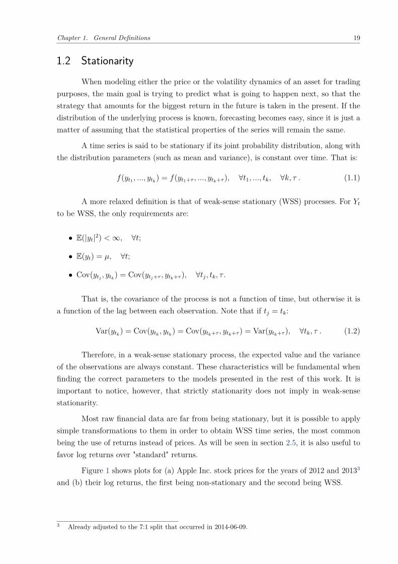
1.2 StationarityWhen modeling either the price or the volatility dynamics of an asset for trading
purposes, the main goal is trying to predict what is going to happen next, so that thestrategy that amounts for the biggest return in the future is taken in the present. If thedistribution of the underlying process is known, forecasting becomes easy, since it is just amatter of assuming that the statistical properties of the series will remain the same.
A time series is said to be stationary if its joint probability distribution, along withthe distribution parameters (such as mean and variance), is constant over time. That is:
f(yt1 , ..., ytk) = f(yt1+τ , ..., ytk+τ ), ∀t1, ..., tk, ∀k, τ . (1.1)
A more relaxed definition is that of weak-sense stationary (WSS) processes. For Ytto be WSS, the only requirements are:
• E(|yt|2) <∞, ∀t;
• E(yt) = µ, ∀t;
• Cov(ytj , ytk) = Cov(ytj+τ , ytk+τ ), ∀tj, tk, τ .
That is, the covariance of the process is not a function of time, but otherwise it isa function of the lag between each observation. Note that if tj = tk:
Var(ytk) = Cov(ytk , ytk) = Cov(ytk+τ , ytk+τ ) = Var(ytk+τ ), ∀tk, τ . (1.2)
Therefore, in a weak-sense stationary process, the expected value and the varianceof the observations are always constant. These characteristics will be fundamental whenfinding the correct parameters to the models presented in the rest of this work. It isimportant to notice, however, that strictly stationarity does not imply in weak-sensestationarity.
Most raw financial data are far from being stationary, but it is possible to applysimple transformations to them in order to obtain WSS time series, the most commonbeing the use of returns instead of prices. As will be seen in section 2.5, it is also useful tofavor log returns over "standard" returns.
Figure 1 shows plots for (a) Apple Inc. stock prices for the years of 2012 and 20133
and (b) their log returns, the first being non-stationary and the second being WSS.
3 Already adjusted to the 7:1 split that occurred in 2014-06-09.

Chapter 1. General Definitions 20
(a) AAPL prices (b) AAPL log returns
Figure 1 – Weak-sense stationarity example
1.3 Linear RegressionEconometrics is a field of economics which seeks to find relationships between
economic variables by employing methods from statistics, mathematics and computerscience. Most of these relationships are studied in the form of linear regressions, becauseestimating their parameters is relatively easy and yet they are powerful enough to describehow most financial variables relate to each other. All the models presented in this workare linear regressions.
A linear regression models how the value of independent variables affects the valueof a dependent variable, having the following general form:
yt = α + β1x1,t + β2x2,t + ...+ βn−1xn−1,t + βnxn,t + εt , (1.3)
or, simply:yt = α +
n∑i=0
βixi,t + εt , (1.4)
where:
• t represents the tth observation of a variable;
• y is the dependent variable;
• xi are the independent variables;
• α is a parameter representing the intercept;
• βi are parameters representing the weight that the values of each xi have in thevalue of y;
• ε is the error, that is εt = yt − α−∑ni=0 βixi,t.

Chapter 1. General Definitions 21
A well known risk measure in the market is the β of an investment (a single securityor a basket), which relates its returns to the returns of a benchmark, often the marketitself. This measure is calculated using a simple linear regression:
rt = α + βrb,t + εt , (1.5)
where r is the return of the investment, and rb is the return of the used benchmark.The noise ε may here be interpreted as an unexplained return, and α is the so calledactive-return of an investment. The investment follows the return of the benchmark by afactor of β, meaning that if the absolute value of this parameter is smaller than one, theinvestment is less volatile than the benchmark.
A good proxy for the market performance may be given by an index, such as thewell known S&P 500. This particular index was used to find a β value of approximately0.98 for Apple Inc. stocks, using data for the years of 2012 and 2013. Details on how toestimate parameters of linear regressions will be briefly discussed in chapter 3.
1.4 High Frequency Financial DataWith the rise of systems capable of rapid performing automated and algorithmic
trading strategies, popularly known as high frequency trading, the amount of data generatedduring a single trading day is enormous, sometimes in a ratio of a trade every millisecond,for each asset. This quantity of available high frequency intraday information allowedresearchers to develop models as the HEAVY model that is studied in this work, becausebefore technology allowed, there were not enough per day data to take advantage from.One of the first major publications in the subject is (GENÇAY et al., 2001).
Sometimes, the expression high frequency financial data refers to all the informationfound in an exchange’s order book, including not only effective trades, but all the bidsand asks that occurred during a day. These may also appear in the literature as ultra highfrequency financial data and can have many practical applications, but they are not thefocus here. A model for the dynamics of the order book applied in the context of HFTwas the subject of a dissertation presented by a previous master student from FundaçãoGetulio Vargas (NUNES, 2013) (in Portuguese).
As for this work, high frequency financial data accounts only for intraday trades.In contrast to daily data, these offer treatment problems of their own (GOODHART;O’HARA, 1997) and different statistical properties, as shown in (CONT, 2001). Everyintraday trade will be accounted as being of high frequency, while daily returns (or anythingwith a smaller granularity) are considered to be of low frequency.

22
2 Mean Models
Even though volatility models may be applied completely separated from meanmodels, a good understanding of the latter is a valuable asset when learning them. Thischapter aims to give the reader a review on the subject.
2.1 Random WalkThe most basic way to model the mean is through a random walk. It is a stochastic
process where the next value of a variable yt is given by its previous value yt−1 plus arandom perturbation. That is:
yt = yt−1 + εt, εti.i.d.∼ N(0, 1) , (2.1)
where εt is an independent and identically normally distributed random variable, withmean 0 and variance 1. An error of this form is also known in the literature as a whitenoise.
This process is a Markov chain, since it has no memory of older values, otherthan the last one. It is also a martingale1, i.e. E(yt+s |Ft) = yt, ∀t, s, so forecasting isimpossible, since the expected value of any future iteration of yt will always be the currentvalue. Figure 2 shows 30 simulations of a random walk process, with y0 = 0, as if it hadbeen observed daily during the years of 2012 and 2013.
Figure 2 – Random walk example
1 Ft is the symbol for σ-algebra, and here it means "all the information available until moment t".

Chapter 2. Mean Models 23
2.2 Autoregressive ModelsAs its name should already suggest, an autoregressive (AR) model of order p is
one of the form:
yt = ω + α1yt−1 + α2yt−2 + ...+ αp−1yt−(p−1) + αpyt−p + εt, εti.i.d.∼ N(0, 1) , (2.2)
or, simply:
yt = ω +p∑i=1
αiyt−i + εt, εti.i.d.∼ N(0, 1) . (2.3)
An AR(p) is then a model where there is an autoregression of the dependentvariable yt by its p past values, yt−1, yt−2, ..., yt−(p−1), yt−p, the independent variables of themodel, with parameters ω, α1, α2, ..., α(p−1), αp.
If the process being modeled is stationary, some conclusions about the possiblevalues of the parameters αi may rise. For simplicity, consider an AR(1) model:
yt = ω + α1yt−1 + εt, εti.i.d.∼ N(0, 1) . (2.4)
If the expectation is taken:
E(yt) = E(ω + α1yt−1 + εt)
= E(ω) + E(α1yt−1) + E(εt)
= E(ω) + E(α1)E(yt−1) + E(εt)
= ω + α1E(yt−1) . (2.5)
For the process to be stationary, E(yt) must be constant, ∀t:
E(yt) = E(yt−1) = µ , (2.6)
hence,E(yt)− α1E(yt−1) = µ(1− α1) = ω , (2.7)
andµ = ω
1− α1. (2.8)
That is, α1 6= 1 and, from (2.7), ω = µ(1− α1):
yt = ω + α1yt−1 + εt
= µ(1− α1) + α1yt−1 + εt
= µ− α1µ+ α1yt−1 + εt , (2.9)
and, finally,yt − µ = α1(yt−1 − µ) + εt . (2.10)

Chapter 2. Mean Models 24
Taking the variance from (2.10):
Var(yt) = α21Var(yt−1) + 1 . (2.11)
Var(yt) should also be constant, ∀t, such that:
Var(yt) = Var(yt−1) = σ2 , (2.12)
hence,Var(yt)− α2
1Var(yt−1) = σ2(1− α21) = 1 , (2.13)
andσ2 = 1
1− α21. (2.14)
Since variance is a positive quantity, |α1| < 1.
2.2.1 Forecasting
When using AR(p) models for forecasting, all one needs to do is to calculate theexpected value of yt s-steps ahead, s being the horizon of prediction, given the informationavailable until the moment. The name mean model comes exactly from this seek for theexpected value, or the mean.
Forecasting yt+3 using an AR(2) model would be:
E(yt+3 |Ft) = E(ω + α1yt+2 + α2yt+1 + εt+3 |Ft)
= ω + α1E(yt+2 |Ft) + α2E(yt+1 |Ft)
= ω + α1E(ω + α1yt+1 + α2yt + εt+2 |Ft) + α2E(ω + α1yt + α2yt−1 + εt+1 |Ft)
= ω + α1ω + α21E(yt+1 |Ft) + α1α2yt + α2ω + α2α1yt + α2
2yt−1
= ω(1 + α1 + α2) + 2α1α2yt + α22yt−1 + α2
1E(yt+1 |Ft)
= ω(1 + α1 + α2) + 2α1α2yt + α22yt−1 + α2
1E(ω + α1yt + α2yt−1 + εt+1 |Ft)
= ω(1 + α1 + α2) + 2α1α2yt + α22yt−1 + α2
1ω + α31yt + α2
1α2yt−1
= ω(1 + α1 + α2 + α21) + 2α1α2yt + α3
1yt + α21α2yt−1 + α2
2yt−1 . (2.15)

Chapter 2. Mean Models 25
A possible Python implementation of 2.15 is:
import numpy
def ar2_forecast(omega, alphas, y_past, steps=1):
"""
Returns the ’steps’−ahead forecast for the AR(2) model."""
y = numpy.zeros(steps + 2)
y[0] = y_past[0]
y[1] = y_past[1]
for i in range(2, steps + 2):
y[i] = omega + alphas[0] ∗ y[i−1] + alphas[1] ∗ y[i−2]
return numpy.copy(y[2:(steps + 2)])
2.3 Moving Average ModelsA moving average (MA) model has a similar structure to an AR model, but instead
of using the past values of the dependent variable as the independent variables, it uses thepast perturbations. A MA(q) model is of the form:
yt = ω + β1εt−1 + β2εt−2 + ...+ βq−1εt−(q−1) + βqεt−q + εt, εti.i.d.∼ N(0, 1) , (2.16)
or, simply:
yt = ω +q∑j=1
βjεt−j + εt, εti.i.d.∼ N(0, 1) . (2.17)
2.4 Autoregressive Moving Average ModelsAn autoregressive moving average (ARMA) model is a union of the two previously
presented models. An ARMA(p, q) has the following form:
yt = ω +p∑i=1
αiyt−i +q∑j=1
βjεt−j + εt, εti.i.d.∼ N(0, 1) . (2.18)

Chapter 2. Mean Models 26
2.5 Autoregressive Integrated Moving Average ModelsWhen a stochastic process Yt is not WSS, one possible way to transform it in one
is to differentiate it. That is, instead of modeling yt, ∆1yt is modeled:
∆1y1 = yt − yt−1 . (2.19)
Two direct implications of this are:
• if ∆1yt is stationary and completely random, ∆1yt = εt, then yt is a random walk;
• if yt is the log price of an asset, ∆1yt represents its log return (as mentioned insection 1.2).
An ARIMA(p, d, q) is a model in which the time series is differentiated d-timesbefore the proper ARMA(p, q) is used. As a consequence, modeling with an ARIMA(p, 0, q)is exactly the same as direct applying an ARMA(p, q).
∆dyt = ω +p∑i=1
αi∆dyt−i +q∑j=1
βjεt−j + εt, εti.i.d.∼ N(0, 1) . (2.20)
The name autoregressive integrated moving average (ARIMA) comes from thefact that if one has a time series generated by this model, it is necessary to "integrate" itd-times in order to obtain a series in the same unit as yt.
2.6 ARIMA with Explanatory Variables ModelsFinally, an ARIMA with explanatory variables (ARIMAX) is an ARIMA with
extra independent variables, which are neither autoregressives nor moving averages:
yt = ω +p∑i=1
αiyt−i +q∑j=1
βjεt−j +n∑k=1
γxk,t + εt, εti.i.d.∼ N(0, 1) , (2.21)
where xk are exogenous variables at instant t, which can be any other variable that areknown to somehow relate to y.
Note that in the equation above yt was used instead of ∆dyt. In favor of notationsimplicity, from now on in this text, it will be assumed that any necessary differentiationis applied to the time series before modeling it (d = 0), since, in practice, it makes nodifference.

27
3 Estimation
Linear regression models were presented in both previous chapters, but until nowno word was said about how to find the right values for each of the model’s parameters.The focus of this chapter is to give an introduction to two of the most used estimationmethods: ordinary least squares and maximum likelihood. A simple AR(1) will be usedto exemplify the application of both of them, but extending the idea to a more complexmodel should not be a problem.
3.1 Ordinary Least SquaresGiven an AR(1) model:
yt = ω + α1yt−1 + εt, εti.i.d.∼ N(0, 1) , (3.1)
and reorganizing the equation:
εt = yt − ω − α1yt−1 . (3.2)
The goal of the Ordinary Least Squares (OLS) method is to find the values ω andα1 for the parameters ω and α1, respectively, that minimize the squared errors, given asample of size T . That is:
argminω,α1
T∑t=2
ε2t = argmin
ω,α1
T∑t=2
(yt − ω − α1yt−1)2 = argminω,α1
f(ω, α1) . (3.3)
Note that the sum starts by the second element, since values for both yt and yt−1
are needed. The estimated parameters ω and α1 will be the solution of the following systemof equations:
δf
δω= −2
T∑t=2
(yt − ω − α1yt−1) = 0 ; (3.4)
δf
δα1= −2
T∑t=2
(yt − ω − α1yt−1)yt−1 = 0 . (3.5)
Solving (3.3) for ω:
−2T∑t=2
(yt − ω − α1yt−1) = 0
T∑t=2
(yt − ω − α1yt−1) = 0
T∑t=2
yt =T∑t=2
ω +T∑t=2
α1yt−1 . (3.6)

Chapter 3. Estimation 28
Rewriting:T∑t=2
yt = ωT∑t=2
1 + α1
T∑t=2
yt−1 . (3.7)
Now, dividing both sides by (T − 1):
T∑t=2
ytT − 1 = ω
T∑t=2
1T − 1 + α1
T∑t=2
yt−1
T − 1 . (3.8)
Being x = ∑ni=1
xi
n(the sample mean), it is possible to simplify (3.8):
yt = ω + α1yt−1 , (3.9)
and finally find the right value for ω:
ω = yt − α1yt−1 . (3.10)
Now, substitute ω in (3.3):
argminω,α1
T∑t=2
[yt − (yt − α1yt−1)− α1yt−1]2
argminω,α1
T∑t=2
[yt − yt + α1yt−1 − α1yt−1]2
argminω,α1
T∑t=2
[(yt − yt)− α1(yt−1 − yt−1)]2 . (3.11)
Differentiating and solving for α1:
−2T∑t=2
[(yt − yt)− α1(yt−1 − yt−1)](yt−1 − yt−1) = 0
T∑t=2
[(yt − yt)− α1(yt−1 − yt−1)](yt−1 − yt−1) = 0
T∑t=2
(yt − yt)(yt−1 − yt−1)− α1(yt−1 − yt−1)2 = 0
α1 =∑Tt=2(yt − yt)(yt−1 − yt−1)
(yt−1 − yt−1)2 = Cov(yt, yt−1)Var(yt−1) . (3.12)
In section 1.3 the β measure was presented. To estimate its value using the OLSmethod, it is as simple as doing:
β = Cov(r, rb)Var(rb)
. (3.13)

Chapter 3. Estimation 29
3.2 Maximum-LikelihoodGiven an AR(1) model:
yt = ω + α1yt−1 + εt, εti.i.d.∼ N(0, 1) , (3.14)
and a sample y1, y2, ..., yT−1, yT of size T . If the sample observations are assumed to beindependent and identically distributed, it is known that the joint probability distributionof them is equal to the product of the their individual distributions, given the parametersω and α1:
f(y2, ..., yT−1, yT |ω, α1) = f(y2 |ω, α1)× ...× f(yT−1 |ω, α1)× f(yT |ω, α1) . (3.15)
Since the presented models assume a distribution for the perturbation term (whichis actually unknown), the objective of the maximum-likelihood estimation (MLE) is tofind parameter values that make the sample distribution match the assumed one. For this,the likelihood function is defined as:
`(ω, α1 ; y2, ..., yT ) , (3.16)
where ω and α1 are variable parameters and y2, ..., yT are fixed parameters. The goal is tofind values for ω and α1 to which:
`(ω, α1 ; y2, ..., yT ) = f(y2, ..., yT |ω, α1) =T∏t=2
f(yt |ω, α1) . (3.17)
In order to do that, we maximize `, and that is the reason the method is calledmaximum-likelihood. Given that all the sample is available, ∀t ≥ 1:
E(yt |Ft−1) = E(ω + α1yt−1 + εt |Ft−1)
= ω + α1yt−1 , (3.18)
andVar(yt |Ft−1) = Var(ω + α1yt−1 + εt |Ft−1) = 1 . (3.19)
Assuming that εt is a white noise:
`(ω, α1 ; y2, ..., yT ) =T∏t=2
f(yt | ω, α1)
=T∏t=2
1√2π
exp[−(yt − ω − α1yt−1)2
2
]. (3.20)
The MLE estimates ω and α1 will be given by:
argmaxω,α1
`(ω, α1 ; y2, ..., yT ) . (3.21)

Chapter 3. Estimation 30
Since the maximum of a product may be very difficult to solve by hand, and maycause floating point problems in a computer, it is usual to calculate the maximum ofthe log-likelihood function. The result is the same, since log is a strictly monotonicallyincreasing function.
argmaxω,α1
ln `(ω, α1 ; y2, ..., yT ) = argmaxω,α1
T∑t=2
ln{
1√2π
exp[−(yt − ω − α1yt−1)2
2
]}
= argmaxω,α1
T∑t=2
ln(
1√2π
)−[
(yt − ω − α1yt−1)2
2
]
= argmaxω,α1
T∑t=2
ln 1− ln√
2π −[
(yt − ω − α1yt−1)2
2
]
= argmaxω,α1
T∑t=2
12 ln 2π −
[(yt − ω − α1yt−1)2
2
]
= argmaxω,α1
T∑t=2
12[ln 2π − (yt − ω − α1yt−1)2] . (3.22)
The estimated parameters ω and α1 will be the solution of the following system ofequations:
δf
δω=
T∑t=2
(yt − ω − α1yt−1) = 0 ; (3.23)
δf
δα1=
T∑t=2
(yt − ω − α1yt−1)yt−1 = 0 . (3.24)
Which, in this case, yield exactly the same results as the ones of the OLS method,(3.10) and (3.12).
It is important to mention, though, that in both methods, after finding the valuesfor ω and α1, one would still need to show that they are in fact a minimum point, in caseof OLS, or a maximum point, in case of MLE, of the their respective objective functions.This can be accomplished by simply differentiating the function again and will not beshown here.

Part II
Volatility Models

32
4 GARCH Family
Following the study of mean models, part II focuses completely on volatility models,and this chapter is responsible for introducing the most known and used family of dailyvolatility models in the market (when one seeks for something more robust than juststandard deviations). Afterwards, GARCH models will be used as benchmarks in the testsof chapter 9.
Up until this point, it was assumed that the variable being modeled could be anyone. From now on, the text will implicitly assume that the variable of interest is thevolatility of returns of a given asset.
4.1 ARCHIntroduced in (ENGLE, 1982), the autoregressive conditional heteroskedasticity
(ARCH) model attempts to give a dynamics to the perturbations of the mean models,other than just assuming they are all white noises. A proper definition of an ARCH oforder q is of the following form:
εt = σtηt, ηti.i.d.∼ N(0, 1) , (4.1)
σ2t = ω + α1ε
2t−1 + α2ε
2t−2 + ...+ αq−1ε
2t−(q−1) + αqε
2t−q . (4.2)
In order to find the right parameters to this model, though, it has to be combinedwith a mean model, like the ones from chapter 2, so that finding values for εt, ∀t, becomesfeasible. If it is the desire of the user to use it standalone, as it was in this work, one needsto assume the log prices of the underlying asset to be random walks, so that their logreturns are given only by:
rt = εt . (4.3)
This way, ARCH may be simplified to:
rt = σtηt, ηti.i.d.∼ N(0, 1) , (4.4)
σ2t = ω +
q∑j=1
αjr2t−j , (4.5)
and anyone can use it to model and forecast volatility without properly modeling rt.
If historical price information is available, it is possible to ignore (4.1) completely,using returns to directly model their volatility with (4.5). The sections that follow willassume this is the only goal, and no attention will be given to the possible dynamics rtmay have: GARCH and its variants will be presented only with the equation for σ2
t . Amore formal definition would require one to explicitly write the equation of εt as well.

Chapter 4. GARCH Family 33
4.2 GARCHAlthough ARCH was the first model of this family, the generalized autoregressive
conditional heteroskedasticity (GARCH) (BOLLERSLEV, 1986) is the most known one.The main difference from its predecessor is that it employs an AR-like dynamics to themodel. A GARCH(p, q) may be specified as:
σ2t = ωG + αG,1r
2t−1 + αG,2r
2t−2 + ...+ αG,q−1r
2t−(q−1) + αG,qr
2t−q
+ βG,1σ2t−1 + βG,2σ
2t−2 + ...+ βG,p−1σ
2t−(p−1) + βG,pσ
2t−p , (4.6)
or, simply:
σ2t = ωG +
q∑j=1
αG,jr2t−j +
p∑i=1
βG,iσ2t−i . (4.7)
Therefore, in this model, σ2t is a regression of the q past values of r2 plus an
autoregression (AR) of its own p past values, with parameters ωG, αG,1, ..., αG,q, βG,1, ..., βG,p.The subscripted G will be important later when differentiating the estimated parametersin the experiments, since the Greek letters ω, α, β are used across all models which willbe tested. Choosing different letters would probably just cause more confusion, so thesubscript will be adopted from now on.
Like it was done before with the AR model, if Rt is supposed to be WSS, itis possible to find restrictions to the possible values of αG,j, βG,i as well. Consider aGARCH(1, 1) model:
σ2t = ωG + αG,1r
2t−1 + βG,1σ
2t−1 . (4.8)
Taking the expectation of σ2t is the same as taking the variance of r:
E(σ2t ) = E(ωG + αG,1r
2t−1 + βG,1σ
2t−1)
= E(ωG) + E(αG,1r2t−1) + E(βG,1σ2
t−1)
= E(ωG) + E(αG,1)E(r2t−1) + E(βG,1)E(σ2
t−1)
= ωG + αG,1E(r2t−1) + βG,1E(σ2
t−1) . (4.9)
From (4.4), it is known that E(r2t ) = E(σ2
t ) and, for the process to be stationary,E(σ2
t ) must be a constant, ∀t:
E(σ2t ) = E(σ2
t−1) = E(r2t−1) = σ2 , (4.10)
hence,E(σ2
t )− αG,1E(r2t−1)− βG,1E(σ2
t−1) = σ2(1− αG,1 − βG,1) = ωG , (4.11)
andσ2 = ωG
1− αG,1 − βG,1. (4.12)
Since variance is a positive quantity, ωG, αG,1, βG,1 > 0 and (αG,1 + βG,1) < 1.

Chapter 4. GARCH Family 34
4.2.1 Estimating
For all the models that are going to be used in the experiments of chapter 9, theMLE was the method of choice to estimate the parameters. Since GARCH will be used inits GARCH(1, 1) form, this will be the example here.
Remember that, the objective of this method is to find values for ωG, αG,1, andβG,1 to which:
`(ωG, αG,1, βG,1 ; r2, ..., rT ) = f(r2, ..., rT |ωG, αG,1, βG,1)
=T∏t=2
f(rt |ωG, αG,1, βG,1) . (4.13)
Given that all the sample is available, ∀t ≥ 1:
E(rt |Ft−1) = E(σtηt |Ft−1) = 0 , (4.14)
and
Var(rt |Ft−1) = Var(σtηt |Ft−1)
= E(σ2t |Ft−1)
= E(ω + αG,1r2t−1 + βG,1σ
2t−1 |Ft−1)
= ωG + αG,1r2t−1 + βG,1σ
2t−1 . (4.15)
Assuming that ηt is a white noise:
`(ωG, αG,1, βG,1 ; r2, ..., rT ) =T∏t=2
f(rt | ωG, αG,1, βG,1) , (4.16)
which is equal to:
T∏t=2
1√2π(ωG + αG,1r2
t−1 + βG,1σ2t−1)
exp[− r2
t
2(ωG + αG,1r2t−1 + βG,1σ2
t−1)
]. (4.17)
The MLE estimates ωG, αG,1, and βG,1 will be given by:
argmaxωG,αG,1,βG,1
`(ωG, αG,1, βG,1 ; r2, ..., rT ) . (4.18)
The last part of the procedure is quite similar the one presented in section 3.2. In acomputer, one may use an optimizer to find the maximum-likelihood estimator for each ofthe parameters. This will be exemplified in subsection 6.1.1 with the HEAVY model, butthe same method is easily adapted to work with GARCH and the source code is availablein annex A.

Chapter 4. GARCH Family 35
4.2.2 Forecasting
If one wants to know the probable value σ2t will have s-steps ahead in the future,
as with the AR model, all that is necessary is to calculate its expected value.
Forecasting σ2t+3 using a GARCH(1, 1) model then is:
E(σ2t+3 |Ft) = E(ωG + αG,1r
2t+2 + βG,1σ
2t+2 |Ft)
= ωG + αG,1E(r2t+2 |Ft) + βG,1E(σ2
t+2 |Ft)
= ωG + αG,1E(σ2t+2 |Ft) + βG,1E(σ2
t+2 |Ft)
= ωG + (αG,1 + βG,1)E(σ2t+2 |Ft)
= ωG + (αG,1 + βG,1)E(ωG + αG,1r2t+1 + βG,1σ
2t+1 |Ft)
= ωG + (αG,1 + βG,1)[ωG + αG,1E(r2t+1 |Ft) + βG,1E(σ2
t+1 |Ft)]
= ωG + (αG,1 + βG,1)[ωG + αG,1E(σ2t+1 |Ft) + βG,1E(σ2
t+1 |Ft)]
= ωG + (αG,1 + βG,1)[ωG + (αG,1 + βG,1)E(σ2t+1 |Ft)]
= ωG + ωG(αG,1 + βG,1) + (αG,1 + βG,1)2E(σ2t+1 |Ft)
= ωG(1 + αG,1 + βG,1) + (αG,1 + βG,1)2E(σ2t+1 |Ft)
= ωG(1 + αG,1 + βG,1) + (αG,1 + βG,1)2E(ωG + αG,1r2t + βG,1σ
2t |Ft)
= ωG(1 + αG,1 + βG,1) + (αG,1 + βG,1)2(ωG + αG,1r2t + βG,1σ
2t ) . (4.19)
Since (αG,1 + βG,1) < 1, σ2t will slowly, but surely, mean revert. The algorithm
to compute such forecast will also be left to be exemplified in subsection 6.1.2, for theHEAVY case. Again, the same method is easily adapted to work with GARCH and thesource code is available in annex A.
4.3 IGARCHThe Integrated Generalized Autoregressive Conditional Heteroskedasticity (IGARCH)
looks exactly like a standard GARCH:
σ2t = ωIG +
q∑j=1
αIG,jr2t−j +
p∑i=1
βIG,iσ2t−i , (4.20)
but it is in fact a restricted version of it, where parameters αIG,j and βIG,i sum up to one:
q∑j=1
αIG,j +p∑i=1
βIG,i = 1 . (4.21)
The motivation behind it is to persist the model shocks in the conditional variance,so that they remain important while forecasting (BOLLERSLEV; ENGLE, 1993). Asshould be concluded from (4.12), with IGARCH, the stochastic process Rt (for which
Chapter 4. GARCH Family 36
rt, ∀t > 0, are the realizations) is not WSS. (NELSON, 1990) shows, however, that fora GARCH(1,1)-generated process to be strictly stationary, the necessary condition isE[ln(αG,1η2
t + βG,1)] < 0, a weaker condition than E(αG,1η2t + βG,1) < 1.
Given (4.21), when q = p = 1, it is possible to rewrite:
σ2t = ωIG + αIG,1r
2t−1 + (1− αIG,1)σ2
t−1 . (4.22)
The letters IG will be used to designate IGARCH parameters.
4.4 GARCH with Explanatory VariablesA GARCH with Explanatory Variables (GARCHX) is to GARCH as ARIMAX is
to ARIMA: a GARCH with extra independent variables, which are neither past values ofrt nor of σ2
t :
σ2t = ωGX +
q∑j=1
αGX,jr2t−j +
p∑i=1
βGX,iσ2t−i +
n∑k=1
γGXxk,t . (4.23)
As it will be further seen in chapter 9, this model will be specially useful to producea joint GARCH-HEAVY model, so that one is able to evaluate which of the two is moredescriptive of the daily volatility of the security in question. The letters GX will be usedto designate GARCHX parameters.
4.5 GJR-GARCHThe idea behind the GARCH extension proposed in (GLOSTEN; JAGANNATHAN;
RUNKLE, 1993) is that future increases in the volatility of returns are associated withpresent falls in asset prices. To capture this statistical leverage effect, the three authorswhich gave their initials to the name of the GJR-GARCH model propose the following:
σ2t = ωGJR +
q∑j=1
αGJR,jr2t−j +
o∑k=1
γGJR,kr2t−kIt−k +
p∑i=1
βGJR,iσ2t−i , (4.24)
with It = 1 if rt < 1, and It = 0 otherwise, ∀t. Adding a new term to the equation everytime a negative return occurred in the past, heightening the effect squared returns have inthe resulted volatility.
Since it is not possible to predict whether a negative return will happen, whenforecasting with an horizon of size s, s > 1, the evaluations from chapter 9 will assume:
E(It+s |Ft) = E(It+s) ≈12 , (4.25)
causing the constraints to this models’ parameters to be slightly different from the onesfrom GARCH. In the GJR-GARCH(1,1,1) case:
(αGJR,1 + γGJR,1
2 + βGJR,1)< 1.

37
5 Realized Measures
After presenting the most known GARCH models, the concept of realized measures(RM) need to be explained before continuing, because they are in the heart of the HEAVYmodels, which are the focus of this work and will be presented in the next chapter.
As GARCH used the daily returns of an asset, rt, as its main source of information,the respective realized measures, RMt, are what HEAVY utilizes. They are nonparametric-based estimators of the variance of a security in a day, which, as opposed to r2
t , ignoreovernight effects, and sometimes even the variation of the first moments of a given day,since these may be regarded as more noisy than the rest of the trading session.
Both (BARNDORFF-NIELSEN; SHEPHARD, 2006) and (ANDERSEN; BOLLER-SLEV; DIEBOLD, 2002) give a background on the subject, and the idea here is only topresent the realized measures that were used during the tests with the HEAVY family ofmodels in this work.
5.1 Realized VarianceThe most simply of the realized measures, realized variance (RV), is the given by
the sum of intraday squared returns. If pτ is the log price of an asset at instant τ , then:
RMt = RVt =nt∑τ=1
(pτ − pτ−1)2 , (5.1)
where nt is the number of used intraday prices within day t. As already pointed out insection 1.1, ∆τ , the interval between each observation, needs to be a constant to allowequal treatment for each pτ . In this work, a ∆τ of five minutes (300s) was used. The sourcecode for the Python implementation of RVt, given a intraday time series ts, follows:
import numpy
import pandas
def realized_variance(ts, delta=300, base=0):
ts = ts.resample(rule=(str(delta) + ’s’), how=’last’, fill_method=’pad’,
base=base)
ts = numpy.diff(ts)
ts = numpy.power(ts, 2.0)
return sum(ts)

Chapter 5. Realized Measures 38
5.2 Multiscale Realized VarianceThe microstructure of the market may be very noisy in practice, and there are
several studies available that propose estimators to mitigate this effect. Some examplesare: pre-averaging (JACOD et al., 2009); realized kernels (BARNDORFF-NIELSEN et al.,2008); two scale realized variance (ZHANG; MYKLAND; AÏT-SAHALIA, 2005); and itssuccessor, the multiscale realized variance (MSRV), presented in (ZHANG et al., 2006).The latter was chosen given its simplicity of implementation.
Given realized variances of different scales, K:
RV Kt = 1
K
nt∑τ=K+1
(pτ − pτ−K)2 . (5.2)
The MSRVt is defined as:
RMt = MSRVt =Mt∑i=1
αiRVit , (5.3)
where Mt is the quantity of averaged scales, with its optimal value for a sample of size ntbeing in the order of O(√nt). The weights αi are defined as:
αi = 12iM2
t
iMt− 1
2 −1
2Mt
1− 1M2
t
, (5.4)
and the MSRV as whole may be implemented as follows:
from numpy.core.umath import floor, subtract
import numpy
import pandas
def multiscale_realized_variance(ts, delta=300, base=0):
result = 0.0
ts = ts.resample(rule=(str(delta) + ’s’), how=’last’, fill_method=’pad’,
base=base)
m = int(floor(numpy.sqrt(len(ts))))
m2 = numpy.power(m, 2.0)
for i in range(1, m + 1):
scaled_ts = subtract(ts[i:len(x)], x[0:len(ts)−i])scaled_ts = numpy.power(scaled_ts , 2.0)
result += ((sum(scaled_ts) / i) ∗ 12.0 ∗ (i / m2)∗ (((i / m) − 0.5 − (1.0 / (2.0 ∗ m)))/ (1.0 − (1.0 / m2))))
return result
Chapter 5. Realized Measures 39
5.3 "Realized EWMA"Normally used to measure daily volatility, the exponentially weighted moving
average (EWMA) is a special case of IGARCH(1, 1), where ωIG = 0, and has the form:
σ2t = (1− λ)r2
t−1 + λσ2t−1 . (5.5)
However, the name EWMA is commonly associated in the market to a particularimplementation of this model, the one from RiskMetricsTM(MORGAN, 1996), which setsλ = 0.94.
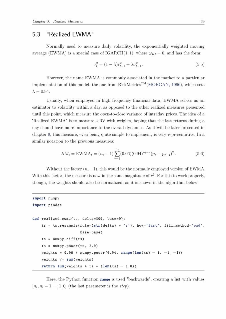
Usually, when employed in high frequency financial data, EWMA serves as anestimator to volatility within a day, as opposed to the other realized measures presenteduntil this point, which measure the open-to-close variance of intraday prices. The idea of a"Realized EWMA" is to measure a RV with weights, hoping that the last returns during aday should have more importance to the overall dynamics. As it will be later presented inchapter 9, this measure, even being quite simple to implement, is very representative. In asimilar notation to the previous measures:
RMt = EWMAt = (nt − 1)nt∑τ=1
(0.06)(0.94)nt−τ (pτ − pτ−1)2 . (5.6)
Without the factor (nt−1), this would be the normally employed version of EWMA.With this factor, the measure is now in the same magnitude of r2. For this to work properly,though, the weights should also be normalized, as it is shown in the algorithm below:
import numpy
import pandas
def realized_ewma(ts, delta=300, base=0):
ts = ts.resample(rule=(str(delta) + ’s’), how=’last’, fill_method=’pad’,
base=base)
ts = numpy.diff(ts)
ts = numpy.power(ts, 2.0)
weights = 0.06 ∗ numpy.power(0.94, range(len(ts) − 1, −1, −1))weights /= sum(weights)
return sum(weights ∗ ts ∗ (len(ts) − 1.0))
Here, the Python function range is used "backwards", creating a list with values[nt, nt − 1, ..., 1, 0] (the last parameter is the step).

Chapter 5. Realized Measures 40
5.4 SubsamplingAnother way to diminish the effect of microstructure noise is to average across
subsamples. This is achieved by simply changing the start point of the sampling process:instead of counting intervals of size ∆τ from the beginning of the trading day, theseintervals begin after a delay of fifteen or thirty seconds (or any other amount of time).
Subsampling is theoretically always beneficial (HANSEN; LUNDE, 2006) and, likethe authors of HEAVY did with their RV estimator, it was applied in the three realizedmeasures presented in this chapter. This was done using starting points every thirtyseconds, up to four minutes and a half, creating ten different subsamples which were thenaveraged. The values presented for these measures in part III always consider subsampling.
Implementing it is quite easy, as it may be seen from the code bellow. Here, fun maybe the name of any function that calculates a RM, given that they all have the same header.
def subsampling(ts, fun, bins=10, bin_size=30):
result = 0.0
delta = bins ∗ bin_sizefor i in range(bins):
result += fun(ts, delta=delta, base=(i ∗ bin_size))return result / bins
5.5 Realized SemivarianceAs the GJR-GARCH, presented in section 4.5, tries to measure the effect of statisti-
cal leverage, section 6.4 will present an extended version of the HEAVY model which utilizesrealized semivariances (RS) with the same intent. These are realized variances that onlymake use of negative returns (BARNDORFF-NIELSEN; KINNEBROCK; SHEPHARD,2008), that is:
RSt =nt∑τ=1
(pτ − pτ−1)2Iτ , (5.7)
with Iτ = 1 if (pτ − pτ−1) < 1, and Iτ = 0 otherwise, ∀τ 1. Applying the same in themultiscale case would be more tricky, since the weights would have to follow a differentequation. This was not attempted here.
1 Implementing it in both realized variance and "realized EWMA" is quite easy: one just needs to substi-tute the line of code ts = numpy.power(ts, 2.0) by ts = numpy.power(ts[ts < 0.0], 2.0) inboth functions.

41
6 HEAVY Family
This chapter is, finally, responsible for presenting the main subject of this work:the HEAVY family of models. The objective is to measure the efficiency of this familyproposed in (SHEPHARD; SHEPPARD, 2010) as an alternative to GARCH models inthe Brazilian market.
The first two sections that follow present the models experimented in the originalpaper, while the last two sections are dedicated to models that were proposed by theoriginal authors as possible extensions to the standard HEAVY. In chapter 9 all fourvariants will be tested against their GARCH counterparts to check whether they do ordo not stand out in this particular market, as well as if the extensions are really worthapplying.
6.1 HEAVYIn section 4.2, the GARCH(1, 1) was presented as1:
σ2t = ωG + αGr
2t−1 + βGσ
2t−1 . (6.1)
If all the information until moment t is available, it is known that:
Var(rt+1 |FLFt ) = σ2
t+1 = ωG + αGr2t + βGσ
2t , (αG + βG) < 1 , (6.2)
where the superscript LF stands for low frequency, that is, GARCH only makes use ofdaily information of security prices variation.
The high-frequency-based volatility (HEAVY) models are specified as:
Var(rt+1 |FHFt ) = ht+1 = ωH + αHRMt + βHht, βH < 1 ; (6.3)
E(RMt+1 |FHFt ) = µt+1 = ωRM + αRMRMt + βRMµt, (αRM + βRM) < 1 , (6.4)
where (6.3) is named HEAVY-r, which models the close-to-close conditional variance (asGARCH does), and (6.4) is named HEAVY-RM, modeling the open-to-close variation.
Note that, now, the superscript HF is used, from highfrequency, since this familyof models is designed to harness high frequency financial data to predict daily asset returnvolatility. This is accomplished by using one of the realized measures presented in chapter5 as the main source of information, as opposed to square returns, like GARCH.1 For the rest of the text, the index in each parameter is going to be suppressed, since models of higher
order will not be referenced anymore.

Chapter 6. HEAVY Family 42
Another important remark is that if one only needs to do 1-step ahead forecasts,only HEAVY-r is needed, since HEAVY-RM exists only as a companion model for whenmultistep-ahead predictions are necessary.
As it will be seen in chapter 9, when compared to GARCH, HEAVY models differespecially in:
• they typically estimate smaller values for β, with ω being really close to zero, so theytend to be a weighted sum of recent realized measures (having more momentum),while GARCH models normally present longer memory;
• they also tend to adjust faster to changes in the level of volatility, like it can be seenin figure 3 (already using Brazilian data for U.S. Dollar future contracts - HEAVYin black, GARCH in gray).
Figure 3 – HEAVY (in black) vs GARCH (in gray) adjustment to volatility changes
When explaining estimation and forecasting in the HEAVY case, the approachwill be different to that used with GARCH or AR, where mathematical demonstrationswere used. Since the methodology employed in the HEAVY model is quite similar the onefrom its counterpart, here the focus will be in its algorithmic implementation. The heavyrfunction that appear in the two following subsections has this form:
def heavyr(omega, alpha, beta, rm_last, h_last):
h = omega + alpha ∗ rm_last + beta ∗ h_lastreturn h
Chapter 6. HEAVY Family 43
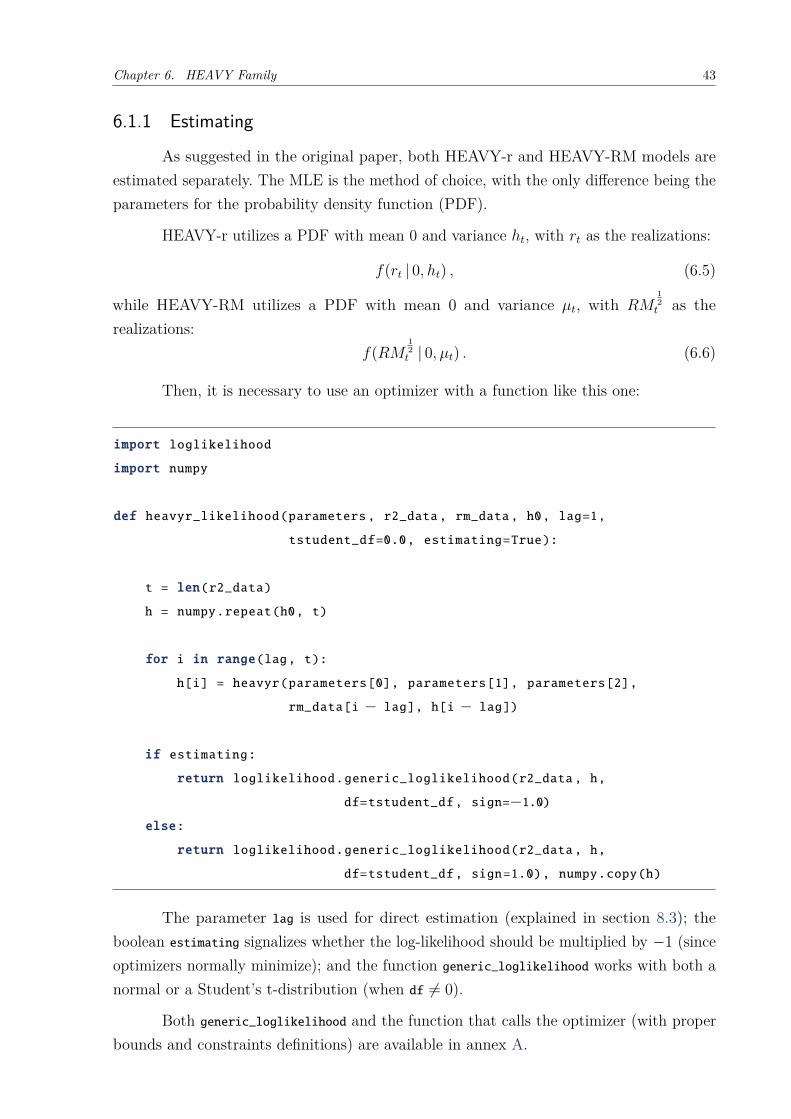
6.1.1 Estimating
As suggested in the original paper, both HEAVY-r and HEAVY-RM models areestimated separately. The MLE is the method of choice, with the only difference being theparameters for the probability density function (PDF).
HEAVY-r utilizes a PDF with mean 0 and variance ht, with rt as the realizations:
f(rt | 0, ht) , (6.5)
while HEAVY-RM utilizes a PDF with mean 0 and variance µt, with RM12t as the
realizations:f(RM
12t | 0, µt) . (6.6)
Then, it is necessary to use an optimizer with a function like this one:
import loglikelihood
import numpy
def heavyr_likelihood(parameters , r2_data, rm_data, h0, lag=1,
tstudent_df=0.0, estimating=True):
t = len(r2_data)
h = numpy.repeat(h0, t)
for i in range(lag, t):
h[i] = heavyr(parameters[0], parameters[1], parameters[2],
rm_data[i − lag], h[i − lag])
if estimating:
return loglikelihood.generic_loglikelihood(r2_data, h,
df=tstudent_df , sign=−1.0)else:
return loglikelihood.generic_loglikelihood(r2_data, h,
df=tstudent_df , sign=1.0), numpy.copy(h)
The parameter lag is used for direct estimation (explained in section 8.3); theboolean estimating signalizes whether the log-likelihood should be multiplied by −1 (sinceoptimizers normally minimize); and the function generic_loglikelihood works with both anormal or a Student’s t-distribution (when df 6= 0).
Both generic_loglikelihood and the function that calls the optimizer (with properbounds and constraints definitions) are available in annex A.
Chapter 6. HEAVY Family 44
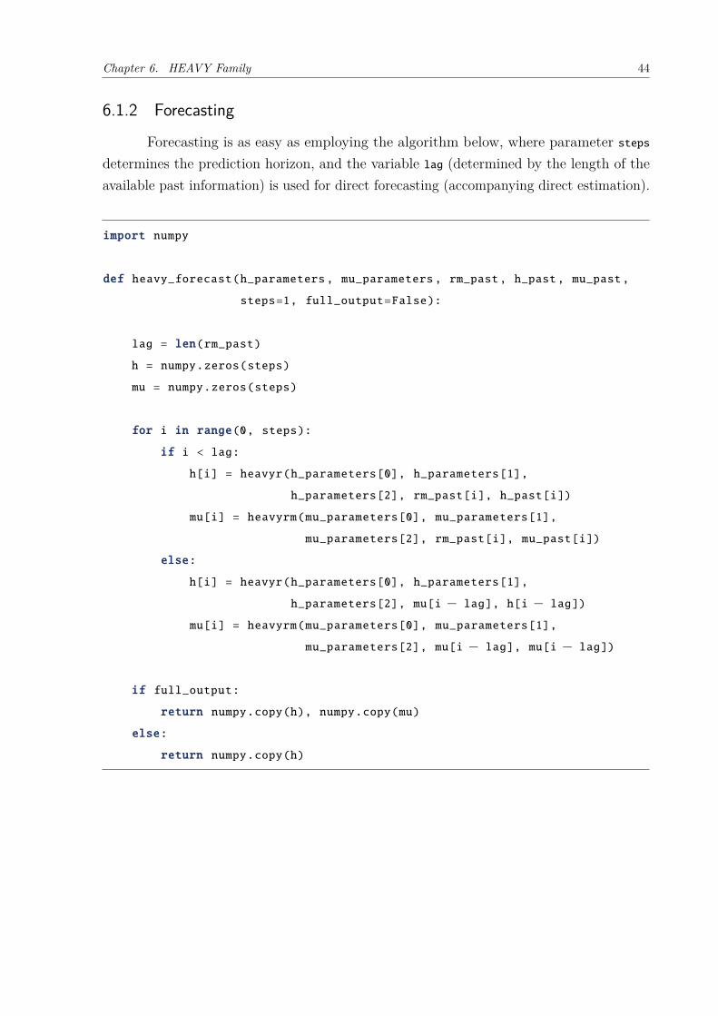
6.1.2 Forecasting
Forecasting is as easy as employing the algorithm below, where parameter stepsdetermines the prediction horizon, and the variable lag (determined by the length of theavailable past information) is used for direct forecasting (accompanying direct estimation).
import numpy
def heavy_forecast(h_parameters , mu_parameters , rm_past, h_past, mu_past,
steps=1, full_output=False):
lag = len(rm_past)
h = numpy.zeros(steps)
mu = numpy.zeros(steps)
for i in range(0, steps):
if i < lag:
h[i] = heavyr(h_parameters[0], h_parameters[1],
h_parameters[2], rm_past[i], h_past[i])
mu[i] = heavyrm(mu_parameters[0], mu_parameters[1],
mu_parameters[2], rm_past[i], mu_past[i])
else:
h[i] = heavyr(h_parameters[0], h_parameters[1],
h_parameters[2], mu[i − lag], h[i − lag])mu[i] = heavyrm(mu_parameters[0], mu_parameters[1],
mu_parameters[2], mu[i − lag], mu[i − lag])
if full_output:
return numpy.copy(h), numpy.copy(mu)
else:
return numpy.copy(h)
Chapter 6. HEAVY Family 45
6.2 Int-HEAVYThe HEAVY family alternative for IGARCH has the following form:
ht = ωIH + αIHRMt−1 + βIHht−1, βIH < 1 ; (6.7)
µt = αIRMRMt−1 + (1− αIRM)µt−1, αIRM < 1 , (6.8)
With (6.7) being exactly equal to (6.3) and changes only happening to HEAVY-RM. Noticethat in this model, not only is αRM + βRM = 1, but the trend parameter ωRM is alsocompletely removed.
6.3 "GJR-HEAVY""GJR-HEAVY" is obviously not how the authors named this model, but on account
of its similarity to GJR-GARCH, this is the name used during the tests to refer to it:
ht = ωGH + αGHRMt−1 + γGHRMt−1It−1 + βGHht−1, βIH < 1 ; (6.9)
µt = ωGRM + αGRMRMt−1 + γGRMRMt−1It−1 + βGRMµt−1,(αGRM + γGRM
2 + βGRM
)< 1 , (6.10)
with It−1 = 1 if rt−1 < 1, and It−1 = 0 otherwise, ∀t, and the same assumption adoptedwith GJR-HEAVY:
E(It+s |Ft) = E(It+s) ≈12 , (6.11)
6.4 Extended HEAVYThis extended version of HEAVY will be referred to as Ext-HEAVY during the
experiments from chapter 9, following the nomenclature choice of the original authors forthe Int-HEAVY model. It uses realized semivariances to accomplish the same statisticleverage effects sought by GJR-GARCH, and that is the reason it will be compared withthis model in the tests (along with "GJR-HEAVY"). It presents the following form:
ht = ωXH + αXHRMt−1 + γXHRSt−1 + βXHht−1, βXH < 1 ; (6.12)
µt = ωXRM + αXRMRMt−1 + βXRMµt−1, (αXRM + βXRM) < 1 ; (6.13)
µ∗t = ωXRS + αXRSRSt−1 + βXRSµ∗t−1, (αXRS + βXRS) < 1 , (6.14)
with (6.14) modeling the open-to-close semivariation.

Part III
Application
47
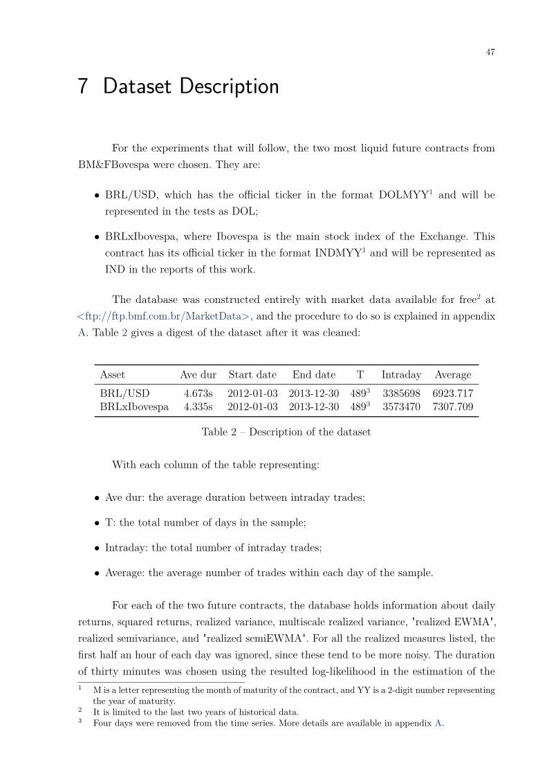
7 Dataset Description
For the experiments that will follow, the two most liquid future contracts fromBM&FBovespa were chosen. They are:
• BRL/USD, which has the official ticker in the format DOLMYY1 and will berepresented in the tests as DOL;
• BRLxIbovespa, where Ibovespa is the main stock index of the Exchange. Thiscontract has its official ticker in the format INDMYY1 and will be represented asIND in the reports of this work.
The database was constructed entirely with market data available for free2 at<ftp://ftp.bmf.com.br/MarketData>, and the procedure to do so is explained in appendixA. Table 2 gives a digest of the dataset after it was cleaned:
Asset Ave dur Start date End date T Intraday AverageBRL/USD 4.673s 2012-01-03 2013-12-30 4893 3385698 6923.717BRLxIbovespa 4.335s 2012-01-03 2013-12-30 4893 3573470 7307.709
Table 2 – Description of the dataset
With each column of the table representing:
• Ave dur: the average duration between intraday trades;
• T: the total number of days in the sample;
• Intraday: the total number of intraday trades;
• Average: the average number of trades within each day of the sample.
For each of the two future contracts, the database holds information about dailyreturns, squared returns, realized variance, multiscale realized variance, "realized EWMA",realized semivariance, and "realized semiEWMA". For all the realized measures listed, thefirst half an hour of each day was ignored, since these tend to be more noisy. The durationof thirty minutes was chosen using the resulted log-likelihood in the estimation of the1 M is a letter representing the month of maturity of the contract, and YY is a 2-digit number representing
the year of maturity.2 It is limited to the last two years of historical data.3 Four days were removed from the time series. More details are available in appendix A.

Chapter 7. Dataset Description 48
models as the metric: without these observations, the function had a higher value in mostcases. They were all also subsampled.
Table 3 shows the summary statistics for each of the measures calculated in thethe dataset:
BRL/USD BRLxIbovespaAvol SD ACF1 Avol SD ACF1
r2 12.746 1.350 0.087 22.499 3.239 −0.011RV 9.764 0.349 0.481 19.442 0.915 0.586MSRV 9.065 0.406 0.472 18.380 1.125 0.331EWMA 8.535 0.326 0.281 16.278 0.866 0.379RS 6.949 0.211 0.389 13.766 0.485 0.556SemiEWMA 6.384 0.183 0.277 12.297 0.426 0.499
Table 3 – Summary statistics for the dataset
Here, Avol stands for annualized volatility, and is calculated using the following:
Avol =√√√√ 1n
n∑i=1
252xi , (7.1)
for which the squared returns present higher values. This is probably because they accountfor overnight returns, while the other measures do not.
Realized measures, in general, have a much smaller standard deviation (SD), andhave a higher serial correlation4. Note that EWMA, however, stands out from its cousins,since it presents even smaller Avol and SD values, although showing a smaller ACF1. Thesmaller values for the semivariances are expected.
Most of these results are in line with the ones available in the original HEAVYstudy, except that, in their findings, currencies used to have no difference in the Avol valuesfor squared returns and realized measures. Presumably, the overnight effects were slighterfor them. Also, the Avol values for indices were a bit more distant in their difference.
Table 3 was computed in its totality using daily and intraday returns multiplied by100, giving a rough idea of percent change. The experiments in chapter 9 use the samekind of data, to smooth the work of the optimizer. Except for ω, which almost alwaystend to zero, all other parameters should not be affected by applying this technique.
4 ACF1 is the autocorrelation function at lag 1.

49
8 Evaluation Metrics
This chapter will present a brief description of the comparison metrics used duringthe experiments from next chapter. The concepts of direct estimation and forecasting willalso be discussed.
8.1 Likelihood-ratio TestTo measure whether squared returns or realized measures give more information
when describing volatility, the following GARCHX(1, 1, 1) model is built:
σ2t = ωGX + αGXr
2t−1 + βGXσ
2t−1 + γGXRMt−1 , (8.1)
and compared with both GARCH and HEAVY using the likelihood-ratio test:
D = −2 ln(
likelihood for null modellikelihood for alternative model
)= −2 ln(likelihood for null model) + 2 ln(likelihood for alternative model) , (8.2)
where the alternative model has more parameters than the null model. Since a model withmore parameters will always have a likelihood value greater (or at least equal) than amodel with less parameters, this quantity is positive. If the null model has m parametersand the alternative model has n parameters, D has a χ2 probability distribution withn−m degrees of freedom.
In chapter 9 however, the reader will notice that this quantity is being reported asa negative value. This is because the GARCHX model in 8.1 was used as the alternativemodel in the test to give an idea of loss of representativeness, so the absolute value of D,|D|, should be considered when calculating the probability of D.
The studied scenario will always have |D| ∼ χ2(1), and its value should be greaterthan the following values for the test to be accepted with a determined significance level:
χ2(1)95% 96% 97% 98% 99%3.841 4.217 4.709 5.411 6.634
Table 4 – χ2(1) significance levels
Chapter 8. Evaluation Metrics 50
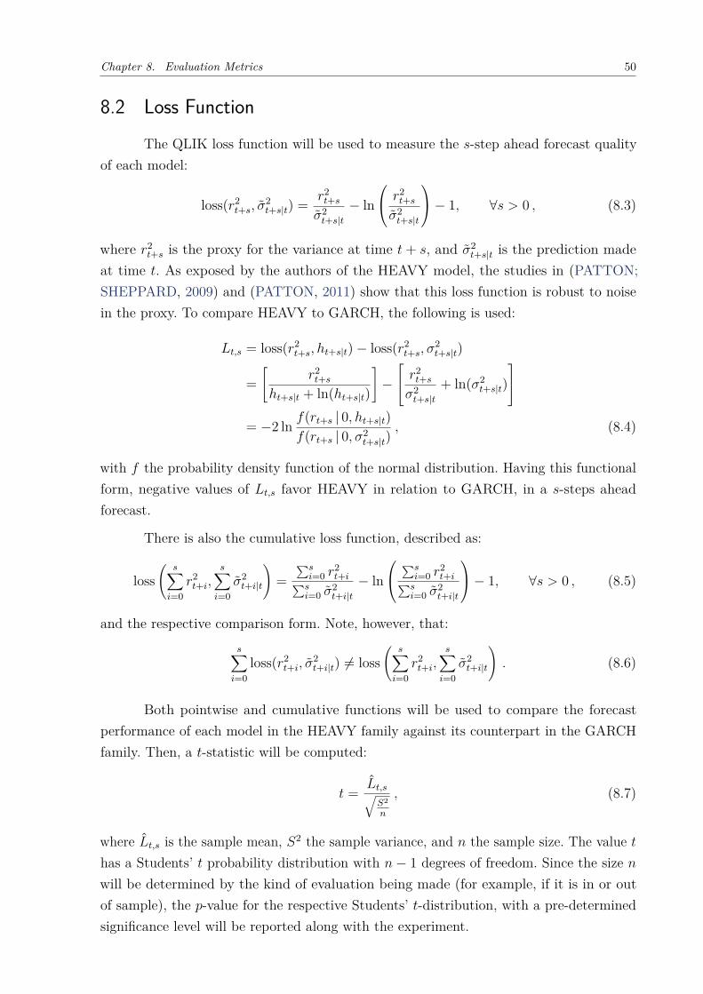
8.2 Loss FunctionThe QLIK loss function will be used to measure the s-step ahead forecast quality
of each model:
loss(r2t+s, σ
2t+s|t) = r2
t+sσ2t+s|t− ln
r2t+s
σ2t+s|t
− 1, ∀s > 0 , (8.3)
where r2t+s is the proxy for the variance at time t + s, and σ2
t+s|t is the prediction madeat time t. As exposed by the authors of the HEAVY model, the studies in (PATTON;SHEPPARD, 2009) and (PATTON, 2011) show that this loss function is robust to noisein the proxy. To compare HEAVY to GARCH, the following is used:
Lt,s = loss(r2t+s, ht+s|t)− loss(r2
t+s, σ2t+s|t)
=[
r2t+s
ht+s|t + ln(ht+s|t)
]−
r2t+s
σ2t+s|t
+ ln(σ2t+s|t)
= −2 ln f(rt+s | 0, ht+s|t)
f(rt+s | 0, σ2t+s|t)
, (8.4)
with f the probability density function of the normal distribution. Having this functionalform, negative values of Lt,s favor HEAVY in relation to GARCH, in a s-steps aheadforecast.
There is also the cumulative loss function, described as:
loss(
s∑i=0
r2t+i,
s∑i=0
σ2t+i|t
)=
∑si=0 r
2t+i∑s
i=0 σ2t+i|t− ln
∑si=0 r
2t+i∑s
i=0 σ2t+i|t
− 1, ∀s > 0 , (8.5)
and the respective comparison form. Note, however, that:s∑i=0
loss(r2t+i, σ
2t+i|t) 6= loss
(s∑i=0
r2t+i,
s∑i=0
σ2t+i|t
). (8.6)
Both pointwise and cumulative functions will be used to compare the forecastperformance of each model in the HEAVY family against its counterpart in the GARCHfamily. Then, a t-statistic will be computed:
t = Lt,s√S2
n
, (8.7)
where Lt,s is the sample mean, S2 the sample variance, and n the sample size. The value thas a Students’ t probability distribution with n− 1 degrees of freedom. Since the size nwill be determined by the kind of evaluation being made (for example, if it is in or outof sample), the p-value for the respective Students’ t-distribution, with a pre-determinedsignificance level will be reported along with the experiment.

Chapter 8. Evaluation Metrics 51
8.3 Direct Estimation and ForecastingNormally, when estimating, one would use the following equation for the volatility
values to be used as input to the PDF in the MLE method (in the HEAVY-r case):
ht = ωH + αHRMt−1 + βHht−1 , (8.8)
and this can be properly used in order to achieve an s-steps ahead forecast. This may, ofcourse, cause loss of information if some time is spent before the parameters are estimatedagain.
From time to time, also, the user of the model already knows in advance that thegoal is to forecast values for an horizon of size s 6= 1. When this happens, it is possible toestimate the values of the parameters with such an horizon in mind. This is called directestimation:
ht = ωH + αHRMt−s + βHht−s . (8.9)
Then, with the right parameter values in hand, direct forecasting can significantlyimprove the results from the desired prediction:
E(ht+s |Ft) = E(ωH + αHRMt + βHht |Ft)
= ωH + αHRMt + βHht . (8.10)
In next chapter, when using the comparison functions presented in section 8.2,both one-step ahead estimation and direct estimation will be used, for different horizonsof prediction.

52
9 Experiments and Results
This final chapter is reserved to present the results from the experiments realizedto compare the effectiveness of the HEAVY model against the GARCH model in theBrazilian market scenario. It is important to make it clear, though, that these results arelimited in scope and should not overlap the results published by the original authors ofthe model.
First, an analysis of the representativeness both realized measures and squaredreturns seem to have in the regression of volatility is shown. Afterwards, each version ofthe HEAVY model presented in chapter 6 will be compared with its GARCH counterpartfrom chapter 4, both in-sample and out-of-sample, using the loss functions presented insection 8.2.
9.1 Realized Measures versus Squared ReturnsTo test whether realized measures or squared returns are more effective in giving
information about the historical values of volatility, a GARCHX model was estimatedusing all three realized measures (each at a time) as exogenous variables. The estimatedparameters appear in table 5:
GARCH GARCHX HEAVY-rAsset RM αG βG αGX βGX γGX αH βH
DOL RV 0.094 0.894 0.000 0.835 0.270 0.270 0.835MSRV 0.000 0.883 0.232 0.232 0.883EWMA 0.000 0.814 0.398 0.398 0.814
IND RV 0.032 0.932 0.000 0.894 0.096 0.096 0.894MSRV 0.000 0.913 0.083 0.084 0.913EWMA 0.007 0.923 0.079 0.087 0.927
Table 5 – Parameters comparison: GARCH x GARCHX x HEAVY-r
In this table, as in all others that will follow up in this chapter, the parametervalues for the GARCH model are shown in the lines corresponding to the RV measure.This is just to avoid the creation of another line just for properly accommodating r2, giventhat it would only be used by this model.

Chapter 9. Experiments and Results 53
Recall from section 8.1 that, here, αGX is the weight for r2t−1 and γGX is the weight
for RMt−1. It is really interesting to see that, apart from the IND + EWMA scenario, allother αGX values are near zero, and, even in this case, it is quite small. The γGX values,on the other hand, are almost identical the values of αH .
Parameter values, however, do not give the whole picture. The likelihood-ratio test,presented in section 8.1, was chosen in order to perform a better verification of this matter.The results are in table 6:
log-likelihood likelihood-ratio testAsset RM GARCH GARCHX HEAVY-r GARCH HEAVY-rDOL RV −550.849 −534.850 −534.850 −31.998 0.000
MSRV −534.940 −534.940 −31.817 0.000EWMA −529.766 −529.766 −42.166 0.000
IND RV −859.615 −856.538 −856.538 −6.153 0.000MSRV −857.139 −857.139 −4.951 0.000EWMA −857.466 −857.544 −4.298 −0.157
Table 6 – Models’ log-likelihood and likelihood-ratio test versus GARCHX
The columns on the left show the log-likelihood value for each of the models, withdifferent realized measures. They are the maximum values found by the optimizer andare negative because, as explained in chapter 7, the intraday returns used to build thetimeseries were multiplied by 100.
The columns on the right show twice the likelihood change for both GARCH andHEAVY when compared to their GARCHX cousins. Note that only the IND + EWMAcombination suffers a small loss in the HEAVY case. This is in line with the parametersvalues in table 5. Nevertheless, when GARCH is compared to GARCHX, the result iscompletely different, and the loss of information is substantial.
From table 4, in section 8.1, it is possible to affirm that the results from table 6, inthe U.S. Dollar case, are statistically significant, with 99% of confidence. In the case ofIbovespa, it is plausible to say, with a significance level of 95%, that the realized measuresdo provide more information than the squared returns, when modeling volatility.

Chapter 9. Experiments and Results 54
9.2 HEAVY versus GARCHFrom the previous section, it is reasonable for one to believe that the forecast
produced by modeling the series of volatility using the HEAVY model would be betterthan doing so with GARCH. This is true in most of the cases, but, in several experiments,the difference is not significant enough for one to be able to affirm this, as it will be seenin the following sections.
First, though, it is interesting to see that the HEAVY parameters are estimatedas promoted. That is, the αH values, presented in table 5, are always higher than the αGvalues. Even in the Ibovespa case, where these values are not even 0.1, they are still aboutthree times higher than αG.
In-Sample
For the in-sample experiments, all the available data points (489) were used forboth sampling and forecasting. This means that, for the tests from section 8.2 to beaccepted with a level of significance of 95%, the absolute value of the computed t-statisticshould be greater than 1.96 in each scenario.
Table 7 presents the results for both pointwise and cumulative loss functions, whencomparing HEAVY to GARCH estimated to perform better at 1-step ahead forecasts. Thenumbers corresponding to the name of each column represent the forecast horizon thatwas utilized in the test. Remember, negative values favor HEAVY.
t > 1.96 Pointwise CumulativeAsset RM 1 2 3 5 10 2 3 5 10DOL RV −2.83 −2.42 −2.23 −2.75 −1.71 −3.54 −4.03 −5.04 −6.23
MSRV −2.95 −2.65 −2.57 −2.39 −1.37 −3.71 −4.26 −4.98 −5.23EWMA −3.04 −2.75 −2.58 −3.28 −2.27 −3.80 −4.30 −5.54 −7.46
IND RV −1.04 −0.66 −0.81 −0.41 0.00 −1.24 −1.49 −1.66 −2.00MSRV −0.91 −0.89 −0.81 −0.38 0.73 −1.28 −1.51 −1.68 −1.47EWMA −0.68 −0.23 −0.25 −0.10 −0.23 −0.71 −0.79 −0.89 −1.63
Table 7 – In-sample: HEAVY x GARCH
One can notice that, for U.S. dollars, the tests indicate that HEAVY really outper-forms GARCH. This is only not true for a horizon of size 10 in the pointwise case, withthe cumulative result for the same horizon being quite convincing.
It is not possible to affirm the same regarding Ibovespa. Even though HEAVYconsistently outperforms GARCH (with the exception of two cases), the difference is neverstatistically significant.

Chapter 9. Experiments and Results 55
When direct estimating (see section 8.3), the results follow the same trend as withthe 1-step ahead estimation:
t > 1.96 PointwiseAsset RM 2 3 5 10DOL RV −3.32 −1.83 −3.12 −1.33
MSRV −2.14 −1.69 −2.24 −0.31EWMA −3.14 −2.86 −2.65 −1.21
IND RV −0.82 −0.49 −1.17 −0.91MSRV −1.06 −0.15 −0.60 −0.03EWMA −0.60 −0.29 −0.85 −0.48
Table 8 – In-sample with direct estimation: HEAVY x GARCH
Here the only difference being that GARCH never outperforms HEAVY.
Out-of-Sample
For the out-of-sample experiments, a moving window of 451 days (roughly one yearand 10 months) was used, so that the other 38 available days could be used as samplefor each of the tested horizons of prediction. This means that, for the tests from section8.2 to be accepted with a level of significance of 95%, the absolute value of the computedt-statistic should be greater than 2.02 in each scenario.
The likelihood-ratio test from section 9.1 and the in-sample results from previoussubsection should indicate that DOL adapts better than IND to the HEAVY models. Thisis not what the out-of-sample experiments show. Table 9 presents the numbers for 1-stepahead estimations of the models:
t > 2.02 Pointwise CumulativeAsset RM 1 2 3 5 10 2 3 5 10DOL RV 0.46 −0.94 −0.59 −1.03 −0.90 −1.46 0.08 0.27 −0.90
MSRV −0.39 −0.39 −0.40 −0.95 −0.11 −0.70 −0.22 −0.29 0.36EWMA −0.45 −0.21 0.44 −0.33 −0.12 −1.08 −0.23 −0.11 0.15
IND RV −0.84 −1.15 −1.68 −0.47 −1.68 −1.56 −2.46 −2.58 −3.47MSRV −1.52 −1.96 −2.23 −1.31 −0.26 −2.46 −3.19 −3.42 −2.89EWMA 0.98 0.64 0.63 0.55 −2.44 0.82 0.46 0.22 −3.22
Table 9 – Out-of-sample: HEAVY x GARCH
This time, then, the statistically different results appear only for Ibovespa. Forboth assets, however, it is possible to find horizons where GARCH outperforms HEAVY.

Chapter 9. Experiments and Results 56
Table 9’s most intriguing combination is, certainly, IND + EWMA: for mosthorizons, GARCH outperforms HEAVY, but in the only true differences, HEAVY is better.This happens in the 10-step ahead prediction, and the reason for this may be the fact thatHEAVY has more momentum than GARCH, which rapidly reverts to the mean.
This conjecture may be further emphasized by table 10: when direct estimationis employed, it becomes impossible to take any conclusions regarding the difference inforecast quality of the models.
t > 2.02 PointwiseAsset RM 2 3 5 10DOL RV −0.71 −0.65 −1.79 −1.57
MSRV −0.17 −0.68 −1.87 −1.49EWMA −0.91 −0.89 −1.31 −1.68
IND RV −1.26 −1.33 −0.70 −1.52MSRV −1.22 −1.61 −0.05 −0.19EWMA 0.75 −0.16 0.07 −1.27
Table 10 – Out-of-sample with direct estimation: HEAVY x GARCH
9.3 Int-HEAVY versus IGARCHSince the Int-HEAVY model resumes to a standard HEAVY model when forecasting
is applied to the same horizon that the model was estimated for, the direct estimationcomparison between it and IGARCH will not be realized. The estimated parameters andrespective log-likelihood values for the in-sample experiments are shown in table 11:
IGARCH Int-HEAVY-rAsset RM αIG ln ` αIH βIH ln `DOL RV 0.104 −551.198 0.273 0.834 −534.850
MSRV 0.232 0.884 −534.940EWMA 0.407 0.811 −529.766
IND RV 0.043 −862.456 0.142 0.827 −856.538MSRV 0.095 0.899 −857.139EWMA 0.098 0.917 −857.544
Table 11 – Parameters and log-likelihood comparison: IGARCH x Int-HEAVY

Chapter 9. Experiments and Results 57
Notice, though, that since the HEAVY-r equation (6.3) is unchanged in Int-HEAVY(6.7), the log-likelihood values are the same as in the standard case, which, in turn, continueto be higher than the respective IGARCH values. The results for both in-sample (table12) and out-of-sample (table 13) experiments are quite similar the ones found in previoussection.
In-Sample
t > 1.96 Pointwise CumulativeAsset RM 2 3 5 10 2 3 5 10DOL RV −2.29 −1.79 −2.26 −0.50 −3.77 −3.99 −4.53 −4.10
MSRV −2.73 −2.47 −1.56 0.65 −3.92 −4.32 −4.60 −1.63EWMA −2.46 −2.20 −3.30 −1.60 −3.78 −4.12 −5.15 −6.47
IND RV −1.48 −1.48 −1.15 −0.93 −2.24 −2.63 −3.17 −3.95MSRV −1.77 −1.42 −1.04 −0.31 −2.14 −2.53 −3.12 −3.57EWMA −1.33 −0.95 −0.86 −1.07 −1.77 −1.99 −2.45 −3.58
Table 12 – In-sample: Int-HEAVY x IGARCH
Out-of-Sample
t > 2.02 Pointwise CumulativeAsset RM 2 3 5 10 2 3 5 10DOL RV −1.00 −0.43 −0.44 −0.84 −1.60 0.29 0.63 0.50
MSRV −0.47 −0.39 −1.37 0.34 −0.72 −0.30 −0.56 0.41EWMA −0.20 0.38 −0.18 −0.03 −1.05 −0.07 0.20 1.12
IND RV −1.46 −1.91 −0.81 −2.04 −2.11 −3.05 −3.35 −4.31MSRV −2.79 −3.10 −1.93 −1.12 −3.56 −4.27 −4.38 −3.99EWMA 0.28 0.15 −0.06 −2.12 0.26 −0.26 −0.90 −4.06
Table 13 – Out-of-sample: Int-HEAVY x IGARCH
9.4 "GJR-HEAVY" versus GJR-GARCHMoving to the models that take into account the fact that future increases in the
volatility of returns may be associated with present falls in asset prices, "GJR-HEAVY"will be now compared to GJR-GARCH. Table 14 shows the estimated parameter valuesfor each of them.

Chapter 9. Experiments and Results 58
GJR-GARCH "GJR-HEAVY-r"Asset RM αGJR γGJR βGJR ln ` αGH γGH βGH ln `DOL RV 0.094 0.000 0.894 −550.849 0.270 0.000 0.835 −534.850
MSRV 0.232 0.000 0.883 −534.940EWMA 0.398 0.000 0.814 −529.766
IND RV 0.000 0.067 0.937 −853.995 0.000 0.206 0.906 −852.374MSRV 0.000 0.177 0.924 −853.000EWMA 0.000 0.206 0.926 −853.544
Table 14 – Parameters and log-likelihood comparison: GJR-GARCH x "GJR-HEAVY"
It is possible to see that these statistical leverage effects are not present in the DOLtime series (at least when modeling it this way), since both γGJR and γGH are estimatedto be zero. One can also note that not even the log-likelihood values are affected, sincethey are exactly the same as the ones from table 6.
In the IND time series, however, the exact opposite effect can be noticed. BothαGJR and αGH are estimated to be zero, and γGH has a much higher value than αH had -with γGJR more than doubling in relation to αG (see table 5).
Also in the Ibovespa case, the log-likelihood for both models substantially increasedwhen compared to the standard models, with the difference between HEAVY and GARCHnarrowing. These changes are possibly the reason behind the in-sample results for INDnot following the pattern from previous findings. The experiments using 1-step aheadestimation here are the first where GARCH truly overcomes HEAVY.
In-Sample
Table 15 shows the results for forecasts using 1-step ahead estimation, while table16 presents the results when using direct estimation. As before, the outcomes that divergefrom the others (from the same asset) are highlighted in gray.
t > 1.96 Pointwise CumulativeAsset RM 1 2 3 5 10 2 3 5 10DOL RV −2.83 −2.42 −2.23 −2.75 −1.71 −2.83 −3.54 −5.04 −6.23
MSRV −2.95 −2.65 −2.57 −2.39 −1.37 −3.71 −4.26 −4.98 −5.23EWMA −3.04 −2.75 −2.58 −3.28 −2.27 −3.80 −4.30 −5.54 −7.46
IND RV −0.58 0.00 −0.11 1.21 1.52 −0.36 −0.26 0.90 2.51MSRV −0.40 −0.13 −0.05 1.20 2.10 −0.33 −0.22 0.85 3.19EWMA −0.15 0.32 0.29 1.19 1.24 0.15 0.35 1.38 2.62
Table 15 – In-sample: "GJR-HEAVY" x GJR-GARCH
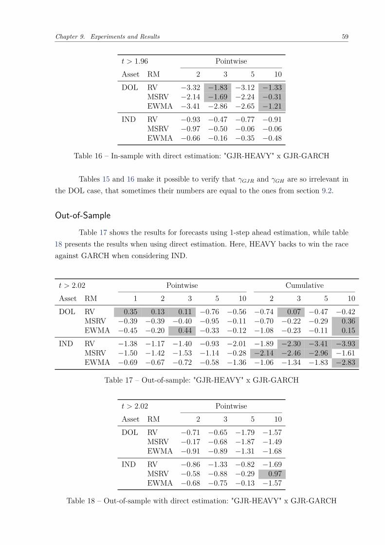
Chapter 9. Experiments and Results 59
t > 1.96 PointwiseAsset RM 2 3 5 10DOL RV −3.32 −1.83 −3.12 −1.33
MSRV −2.14 −1.69 −2.24 −0.31EWMA −3.41 −2.86 −2.65 −1.21
IND RV −0.93 −0.47 −0.77 −0.91MSRV −0.97 −0.50 −0.06 −0.06EWMA −0.66 −0.16 −0.35 −0.48
Table 16 – In-sample with direct estimation: "GJR-HEAVY" x GJR-GARCH
Tables 15 and 16 make it possible to verify that γGJR and γGH are so irrelevant inthe DOL case, that sometimes their numbers are equal to the ones from section 9.2.
Out-of-Sample
Table 17 shows the results for forecasts using 1-step ahead estimation, while table18 presents the results when using direct estimation. Here, HEAVY backs to win the raceagainst GARCH when considering IND.
t > 2.02 Pointwise CumulativeAsset RM 1 2 3 5 10 2 3 5 10DOL RV 0.35 0.13 0.11 −0.76 −0.56 −0.74 0.07 −0.47 −0.42
MSRV −0.39 −0.39 −0.40 −0.95 −0.11 −0.70 −0.22 −0.29 0.36EWMA −0.45 −0.20 0.44 −0.33 −0.12 −1.08 −0.23 −0.11 0.15
IND RV −1.38 −1.17 −1.40 −0.93 −2.01 −1.89 −2.30 −3.41 −3.93MSRV −1.50 −1.42 −1.53 −1.14 −0.28 −2.14 −2.46 −2.96 −1.61EWMA −0.69 −0.67 −0.72 −0.58 −1.36 −1.06 −1.34 −1.83 −2.83
Table 17 – Out-of-sample: "GJR-HEAVY" x GJR-GARCH
t > 2.02 PointwiseAsset RM 2 3 5 10DOL RV −0.71 −0.65 −1.79 −1.57
MSRV −0.17 −0.68 −1.87 −1.49EWMA −0.91 −0.89 −1.31 −1.68
IND RV −0.86 −1.33 −0.82 −1.69MSRV −0.58 −0.88 −0.29 0.97EWMA −0.68 −0.75 −0.13 −1.57
Table 18 – Out-of-sample with direct estimation: "GJR-HEAVY" x GJR-GARCH
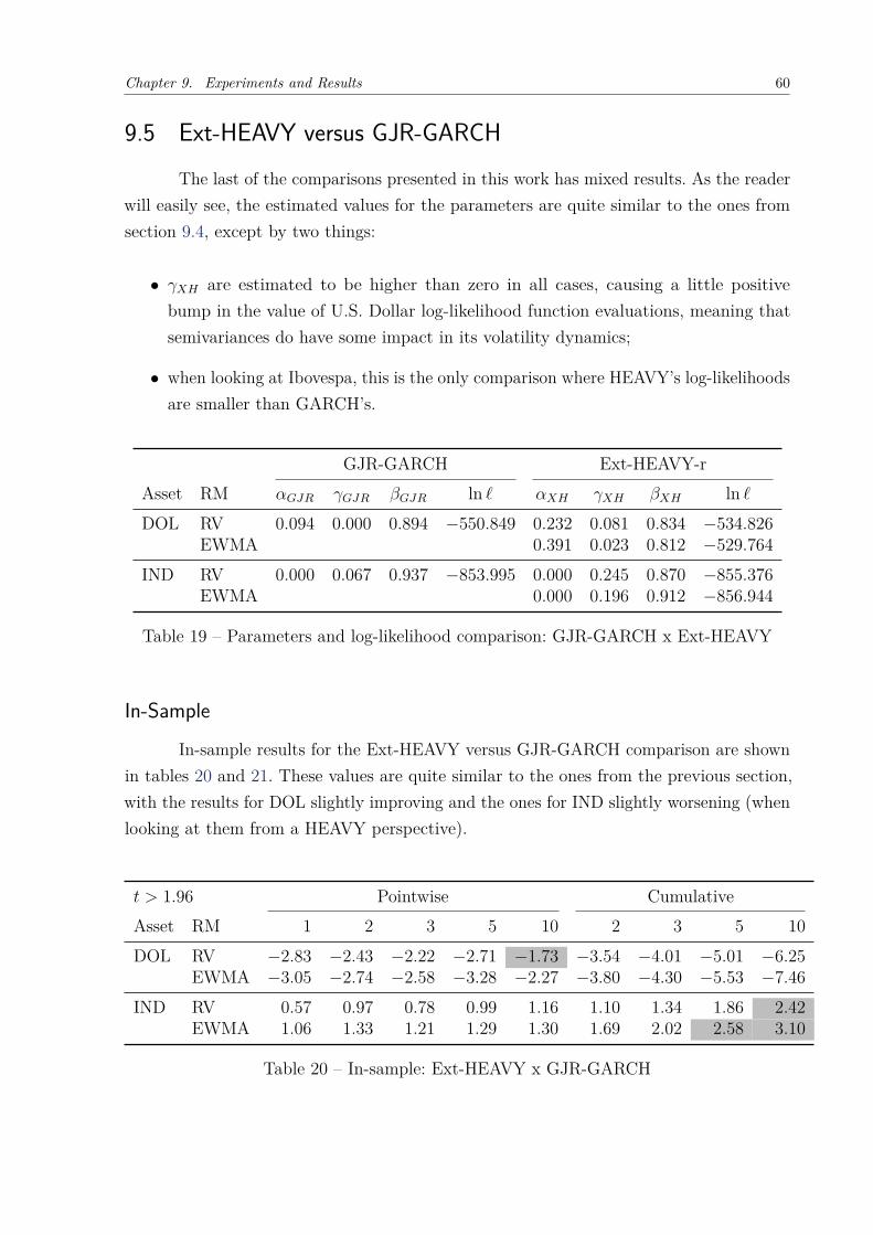
Chapter 9. Experiments and Results 60
9.5 Ext-HEAVY versus GJR-GARCHThe last of the comparisons presented in this work has mixed results. As the reader
will easily see, the estimated values for the parameters are quite similar to the ones fromsection 9.4, except by two things:
• γXH are estimated to be higher than zero in all cases, causing a little positivebump in the value of U.S. Dollar log-likelihood function evaluations, meaning thatsemivariances do have some impact in its volatility dynamics;
• when looking at Ibovespa, this is the only comparison where HEAVY’s log-likelihoodsare smaller than GARCH’s.
GJR-GARCH Ext-HEAVY-rAsset RM αGJR γGJR βGJR ln ` αXH γXH βXH ln `DOL RV 0.094 0.000 0.894 −550.849 0.232 0.081 0.834 −534.826
EWMA 0.391 0.023 0.812 −529.764IND RV 0.000 0.067 0.937 −853.995 0.000 0.245 0.870 −855.376
EWMA 0.000 0.196 0.912 −856.944
Table 19 – Parameters and log-likelihood comparison: GJR-GARCH x Ext-HEAVY
In-Sample
In-sample results for the Ext-HEAVY versus GJR-GARCH comparison are shownin tables 20 and 21. These values are quite similar to the ones from the previous section,with the results for DOL slightly improving and the ones for IND slightly worsening (whenlooking at them from a HEAVY perspective).
t > 1.96 Pointwise CumulativeAsset RM 1 2 3 5 10 2 3 5 10DOL RV −2.83 −2.43 −2.22 −2.71 −1.73 −3.54 −4.01 −5.01 −6.25
EWMA −3.05 −2.74 −2.58 −3.28 −2.27 −3.80 −4.30 −5.53 −7.46IND RV 0.57 0.97 0.78 0.99 1.16 1.10 1.34 1.86 2.42
EWMA 1.06 1.33 1.21 1.29 1.30 1.69 2.02 2.58 3.10
Table 20 – In-sample: Ext-HEAVY x GJR-GARCH
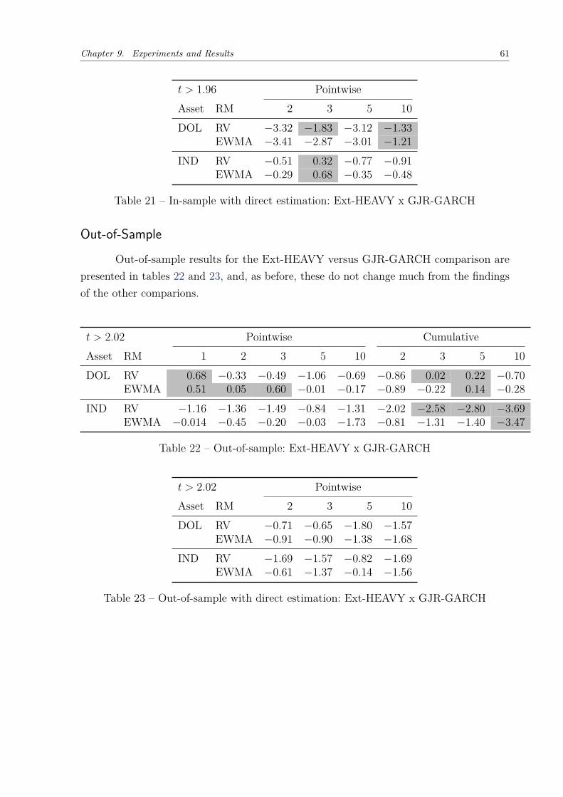
Chapter 9. Experiments and Results 61
t > 1.96 PointwiseAsset RM 2 3 5 10DOL RV −3.32 −1.83 −3.12 −1.33
EWMA −3.41 −2.87 −3.01 −1.21IND RV −0.51 0.32 −0.77 −0.91
EWMA −0.29 0.68 −0.35 −0.48
Table 21 – In-sample with direct estimation: Ext-HEAVY x GJR-GARCH
Out-of-Sample
Out-of-sample results for the Ext-HEAVY versus GJR-GARCH comparison arepresented in tables 22 and 23, and, as before, these do not change much from the findingsof the other comparions.
t > 2.02 Pointwise CumulativeAsset RM 1 2 3 5 10 2 3 5 10DOL RV 0.68 −0.33 −0.49 −1.06 −0.69 −0.86 0.02 0.22 −0.70
EWMA 0.51 0.05 0.60 −0.01 −0.17 −0.89 −0.22 0.14 −0.28IND RV −1.16 −1.36 −1.49 −0.84 −1.31 −2.02 −2.58 −2.80 −3.69
EWMA −0.014 −0.45 −0.20 −0.03 −1.73 −0.81 −1.31 −1.40 −3.47
Table 22 – Out-of-sample: Ext-HEAVY x GJR-GARCH
t > 2.02 PointwiseAsset RM 2 3 5 10DOL RV −0.71 −0.65 −1.80 −1.57
EWMA −0.91 −0.90 −1.38 −1.68IND RV −1.69 −1.57 −0.82 −1.69
EWMA −0.61 −1.37 −0.14 −1.56
Table 23 – Out-of-sample with direct estimation: Ext-HEAVY x GJR-GARCH

62
Conclusion
The main conclusion that this work should lead to, is that the HEAVY family ofmodels are a good alternative to GARCH models. Even though the results with data fromthe Brazilian futures market were not as astonishing as the ones found by the originalstudy, they do provide sufficient reasons to instigate further investigation.
Results such as the ones from section 9.1 show that, although not forecasting muchbetter than GARCH models, the data may fit better with HEAVY. With the experimentsthat followed, there are also evidences that BM&FBovespa’s U.S. Dollar future contractsmay be even better specified with an Ext-HEAVY model, and Ibovespa future contractswith "GJR-HEAVY".
Also, in the experiments involving prediction, even though most of the results werenot necessarily statistically significant, they did give more advantage to HEAVY. Moreover,the use of a larger sample size could enhance the difference produced by the loss functions.In the original paper, the authors used ten years of data, with moving windows of fouryears, but just around a fifth of this amount of information was available for this study.
Still regarding forecasting, in the experiments where most of the results favoredHEAVY, the difference was higher in the cumulative tests with bigger horizons. This canbe related to the fact that HEAVY has more momentum than GARCH, and shows thatHEAVY may be more suitable for longer uses, when the time between reestimations ofthe parameters is considerable.
Finally, one can notice that, during all tests, HEAVY consistently shows betterresults when using EWMA as the realized measure for DOL, and RV for IND. This isinteresting to see, since both estimators are expected to be more noisy than MSRV, andeven so they appear to better describe the volatility of these assets.
Future DirectionsIt was seen that the experiments from chapter 9 were not enough to rigorously
affirm that HEAVY models are superior to GARCH models, or the other way around, atleast in the studied scenario: the 2-year window of those two assets of BM&FBovespa. Ahigher number of assets and a larger sample size would probably suffice.
The ideal sample size for estimation could not be determined as well, and this hasdirect effect in the applicability of any model in a real scenario. One year and 10 monthswas the amount of choice in the out-of-sample experiments both because the availabledata did not permit to use more and because earlier tests with smaller samples showed

Conclusion 63
that the HEAVY parameters estimation was unstable: moving the window one day wouldcause the parameters to change drastically, while moving again could bring them back tothe same level as before.
This was mostly seen with BM&FBovespa’s U.S. Dollar future contract, and,especially, while using realized variances as the realized measure. The multiscale estimatorwas much less sensible, with EWMA staying somewhere in the middle of the two. Thismay be due to the presence of intraday noises in the estimators. Again, the use of moresecurities in the experiments could help answer these questions.
Another point of interest would be comparing the HEAVY models against eachother, to check which one is better. As with GARCH, each of them is probably better forgiven situations, but comparing them would be certainly enlightening.
Further CommentsIt is the hope of the author, that this work served not only to demonstrate the
capabilities of new alternatives when compared to more traditional approaches, but alsothat it has accomplished its goal of encouraging other researchers to explore the Brazilianmarket even more. He also hopes that the reading experience was pleasant and that, ifthis was the first contact of the reader with econometric models, he or she was able tolearn the basics with this text.

64
Bibliography
ANDERSEN, T. G.; BOLLERSLEV, T.; DIEBOLD, F. X. Parametric and nonparametricvolatility measurement. [S.l.]: National Bureau of Economic Research Cambridge, Mass.,USA, 2002.
BARNDORFF-NIELSEN, O. E. et al. Designing realized kernels to measure the ex postvariation of equity prices in the presence of noise. Econometrica, Wiley Online Library,v. 76, n. 6, p. 1481–1536, 2008.
BARNDORFF-NIELSEN, O. E.; KINNEBROCK, S.; SHEPHARD, N. Measuringdownside risk-realised semivariance. CREATES Research Paper, n. 2008-42, 2008.
BARNDORFF-NIELSEN, O. E.; SHEPHARD, N. Variation, jumps and high frequencydata in financial econometrics. Advanced in Economics and Econometrics. Theory andApplications, 2006.
BOLLERSLEV, T. Generalized autoregressive conditional heteroskedasticity. Journal ofEconometrics, Elsevier, v. 31, n. 3, p. 307–327, 1986.
BOLLERSLEV, T.; ENGLE, R. F. Common persistence in conditional variances.Econometrica: Journal of the Econometric Society, JSTOR, p. 167–186, 1993.
CONT, R. Empirical properties of asset returns: stylized facts and statistical issues.Taylor & Francis, 2001.
DACOROGNA, M. M. et al. Modelling short-term volatility with garch and harch models.published by Wiley & Sons, Ltd, 1997.
ENGLE, R. F. Autoregressive conditional heteroscedasticity with estimates of the varianceof united kingdom inflation. Econometrica: Journal of the Econometric Society, JSTOR,p. 987–1007, 1982.
GENÇAY, R. et al. An introduction to high-frequency finance. [S.l.]: Academic Press,2001.
GLOSTEN, L. R.; JAGANNATHAN, R.; RUNKLE, D. E. On the relation between theexpected value and the volatility of the nominal excess return on stocks. The Journal ofFinance, Wiley Online Library, v. 48, n. 5, p. 1779–1801, 1993.
GOODHART, C. A.; O’HARA, M. High frequency data in financial markets: Issues andapplications. Journal of Empirical Finance, Elsevier, v. 4, n. 2, p. 73–114, 1997.
HANSEN, P. R.; LUNDE, A. Realized variance and market microstructure noise. Journalof Business & Economic Statistics, Taylor & Francis, v. 24, n. 2, p. 127–161, 2006.
JACOD, J. et al. Microstructure noise in the continuous case: the pre-averaging approach.Stochastic Processes and their Applications, Elsevier, v. 119, n. 7, p. 2249–2276, 2009.
MORGAN, J. Riskmetrics: technical document. [S.l.]: Morgan Guaranty Trust Companyof New York, 1996.

Bibliography 65
NELSON, D. B. Stationarity and persistence in the garch (1, 1) model. Econometrictheory, Cambridge Univ Press, v. 6, n. 03, p. 318–334, 1990.
NOURELDIN, D.; SHEPHARD, N.; SHEPPARD, K. Multivariate high-frequency-basedvolatility (heavy) models. Journal of Applied Econometrics, Wiley Online Library, v. 27,n. 6, p. 907–933, 2012.
NUNES, G. d. F. C. Modelo da dinâmica de um livro de ordens para aplicações emhigh-frequency trading. 2013.
PATTON, A. J. Volatility forecast comparison using imperfect volatility proxies. Journalof Econometrics, Elsevier, v. 160, n. 1, p. 246–256, 2011.
PATTON, A. J.; SHEPPARD, K. Evaluating volatility and correlation forecasts. In:Handbook of financial time series. [S.l.]: Springer, 2009. p. 801–838.
SCHMIDT, A. B. Financial markets and trading: an introduction to marketmicrostructure and trading strategies. [S.l.]: John Wiley & Sons, 2011.
SHEPHARD, N.; SHEPPARD, K. Realising the future: forecasting with high-frequency-based volatility (heavy) models. Journal of Applied Econometrics, Wiley Online Library,v. 25, n. 2, p. 197–231, 2010.
ZHANG, L.; MYKLAND, P. A.; AÏT-SAHALIA, Y. A tale of two time scales. Journal ofthe American Statistical Association, v. 100, n. 472, 2005.
ZHANG, L. et al. Efficient estimation of stochastic volatility using noisy observations:A multi-scale approach. Bernoulli, Bernoulli Society for Mathematical Statistics andProbability, v. 12, n. 6, p. 1019–1043, 2006.

Appendix

67
APPENDIX A – Database Construction
BM&FBovespa distributes its market data in .csv files, properly accompanied bydescription files that explain what information is contained in the files. In the data thatwere used, from January until August, 2012, there was one file per month, and, afterwards,one file per day. The procedure to transform these files in a useful database (having thiswork in mind) is explained below, divided in three major steps.
The Python scripts that implement each of these steps are available in GitHub(<https://github.com/twalves/dissertation>), under the following names:
• step 0: init_database.py;
• step 1: init_raw_tables.py;
• step 2: init_work_tables.py;
• step 3: init_work_timeseries.py.
Where step 0 refers solely to the creation of the database and auxiliary tables. Ifexecuted in this order, with the proper .csv files in hand, the same database as the oneused in this work should be created. In a machine with a 2.9GHz Intel Core i7 processor,8GB 1600 MHz DDR3 ram memory, and a 5400rpm SATA disk, it takes about 2 hours forthe whole process to complete.
A MySQL1 database was utilized, but since the Python library SQLAlchemy2 wasused, the scripts should work properly with any database engine. Other than these, asthe code snippets that appeared before, the only required external libraries are the mostknown NumPy3 and pandas4.
The procedures executed in each of the above scripts will now be briefly described.
Step 1For all the data available for each month (even if in separate files), create a pandas’
DataFrame object with all the columns available in the original data, then filter the data to:
1. remove all the lines for which the instrument symbol represents neither DOL norIND contracts;
1 <http://www.mysql.com>2 <http://www.sqlalchemy.org>3 <http://www.numpy.org>4 <http://pandas.pydata.org>

APPENDIX A. Database Construction 68
2. remove all the lines for which the trade time is ’00:00:00:000’
3. remove all the lines for which there is no "trade indicator" number
After that, save all the filtered information in the database, to what was calledthe "raw tables", one for each month. When completed, each table should have around500, 000 lines of data (≈ 50MB).
Step 2Since there are different maturities for each of the future contracts used in this
work, the maturity with higher daily volume, per day and per asset, is chosen. Two SQLscripts are used to do the "dirty" work here, using temporary tables. Then, for the selecteddata:
1. the weighted average price is calculated when there is more than one trade withexactly the same timestamp, where the volume from each trade is used as the weight;
2. the log prices are computed;
3. the "instrument symbol" column is divided in three columns: "asset", "month", "year".
The resulted table is saved in the database as a "work table", but now only withthe columns "session date", "trade time", "asset", "month", "year", "trade price", and "logtrade price". Again, a table is created for each month, and now each of them has around250, 000 lines of data (≈ 20MB).
Step 3Only two more tables are created in this step: one for DOL and one for IND.
Each of them containing one line per day, with all the required measures to estimate andevaluate the models presented in this work, using the algorithms suggested in chapter 5.During this step, four days were ignored, due to different reasons:
• 2012-02-22 and 2013-02-13, which are half-day holidays in Brazil that occur everyWednesday after Carnival, when trading begins only after 1pm;
• 2012-02-01, which, for some unknown reason, had no data from 1h02pm until 1h43pm;
• 2012-03-12, which also did not present any values until 9h40am.

Annex

70
ANNEX A – Code Listings
The following source codes constitute a portion of what was produced during thedevelopment of this work. These are the ones that received some kind of reference duringthe text:
• loglikelihood.py: log-likelihood functions for both Gaussian distribution and Stu-dent’s t-distribution;
• heavy.py: HEAVY-r and HEAVY-RM functions for log-likelihood evaluation, estima-tion and forecasting;
• garch.py: GARCH functions for log-likelihood evaluation, estimation and forecasting.
The implementation of all other models used in this work are available in GitHub(<https://github.com/twalves/dissertation>), along with the database creation scriptsmentioned in appendix A. The code listed here is also available online, in its properlycommented version. Here, comments are ommited in order to keep the length as small aspossible.
Most functions are direct translations from the respective mathematical formulae,being quite easy to read and understand. The estimation methods, though, use someassumptions that need to be clarified:
• The value for both h0 and σ20 is set to be the variance of the
√T initial values of the
available time series of returns, where T is the size of the sample;
• The value for µ0 is set to be the average of the√T initial values of the available
time series of realized measures, where T is the size of the sample;
• The initial guess for the parameter values, which is an argument of the optimizingfunction, is built using a brute force algorithm: a grid around the usual values ofeach parameter is constructed.
Apart from the Python libraries already listed in appendix A, the only differentlibrary that appears in the listing below is SciPy1.
1 <http://scipy.org>
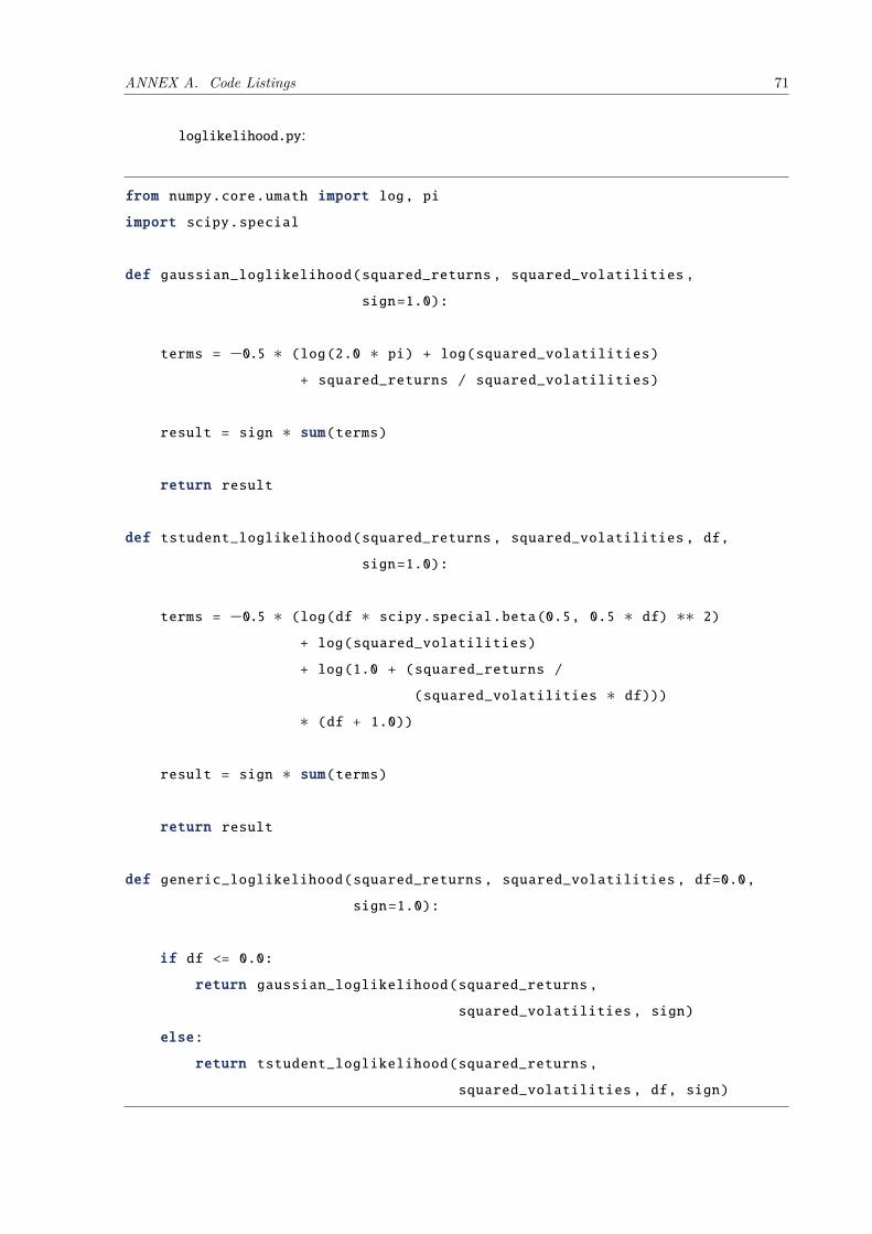
ANNEX A. Code Listings 71
loglikelihood.py:
from numpy.core.umath import log, pi
import scipy.special
def gaussian_loglikelihood(squared_returns , squared_volatilities ,
sign=1.0):
terms = −0.5 ∗ (log(2.0 ∗ pi) + log(squared_volatilities)+ squared_returns / squared_volatilities)
result = sign ∗ sum(terms)
return result
def tstudent_loglikelihood(squared_returns , squared_volatilities , df,
sign=1.0):
terms = −0.5 ∗ (log(df ∗ scipy.special.beta(0.5, 0.5 ∗ df) ∗∗ 2)+ log(squared_volatilities)
+ log(1.0 + (squared_returns /
(squared_volatilities ∗ df)))∗ (df + 1.0))
result = sign ∗ sum(terms)
return result
def generic_loglikelihood(squared_returns , squared_volatilities , df=0.0,
sign=1.0):
if df <= 0.0:
return gaussian_loglikelihood(squared_returns ,
squared_volatilities , sign)
else:
return tstudent_loglikelihood(squared_returns ,
squared_volatilities , df, sign)

ANNEX A. Code Listings 72
heavy.py:
import loglikelihood
import numpy
import time
import scipy.optimize
def heavyr(omega, alpha, beta, rm_last, h_last):
h = omega + alpha ∗ rm_last + beta ∗ h_lastreturn h
def heavyrm(omega, alpha, beta, rm_last, mu_last):
mu = omega + alpha ∗ rm_last + beta ∗ mu_lastreturn mu
def heavy_forecast(h_parameters , mu_parameters , rm_past, h_past, mu_past,
steps=1, full_output=False):
lag = len(rm_past)
h = numpy.zeros(steps)
mu = numpy.zeros(steps)
for i in range(0, steps):
if i < lag:
h[i] = heavyr(h_parameters[0], h_parameters[1],
h_parameters[2], rm_past[i], h_past[i])
mu[i] = heavyrm(mu_parameters[0], mu_parameters[1],
mu_parameters[2], rm_past[i], mu_past[i])
else:
h[i] = heavyr(h_parameters[0], h_parameters[1],
h_parameters[2], mu[i − lag], h[i − lag])mu[i] = heavyrm(mu_parameters[0], mu_parameters[1],
mu_parameters[2], mu[i − lag], mu[i − lag])
if full_output:
return numpy.copy(h), numpy.copy(mu)
else:
return numpy.copy(h)

ANNEX A. Code Listings 73
def heavyr_likelihood(parameters , r2_data, rm_data, h0, lag=1,
tstudent_df=0.0, estimating=True):
t = len(r2_data)
h = numpy.repeat(h0, t)
for i in range(lag, t):
h[i] = heavyr(parameters[0], parameters[1], parameters[2],
rm_data[i − lag], h[i − lag])
if estimating:
return loglikelihood.generic_loglikelihood(r2_data, h,
df=tstudent_df , sign=−1.0)else:
return loglikelihood.generic_loglikelihood(r2_data, h,
df=tstudent_df , sign=1.0), numpy.copy(h)
def heavyrm_likelihood(parameters , rm_data, mu0, lag=1,
tstudent_df=0.0, estimating=True):
t = len(rm_data)
mu = numpy.repeat(mu0, t)
for i in range(lag, t):
mu[i] = heavyrm(parameters[0], parameters[1], parameters[2],
rm_data[i − lag], mu[i − lag])
if estimating:
return loglikelihood.generic_loglikelihood(rm_data, mu,
df=tstudent_df , sign=−1.0)else:
return loglikelihood.generic_loglikelihood(rm_data, mu,
df=tstudent_df , sign=1.0), numpy.copy(mu)

ANNEX A. Code Listings 74
def heavyr_estimate(r2_data, rm_data, lag=1, tstudent_df=0.0,
full_output=True):
before = time.time()
finfo = numpy.finfo(numpy.float32)
h0 = 0.0
t = int(numpy.sqrt(len(r2_data)))
for i in range(t):
h0 += r2_data[i]
h0 /= t
args = (r2_data, rm_data, h0, lag, tstudent_df)
ranges = ((finfo.eps, 0.5), (finfo.eps, 0.5), (0.5, 1.0))
x0 = scipy.optimize.brute(heavyr_likelihood , ranges, args=args,
finish=None)
# Constraint that beta < 1.0constraints = ({’type’: ’ineq’, ’fun’: lambda x: 1.0 − x[2]})
bounds = ((finfo.eps, None), (finfo.eps, None), (finfo.eps, None))
result = scipy.optimize.minimize(heavyr_likelihood , x0, args=args,
method=’SLSQP’, bounds=bounds,
constraints=constraints)
estimates = result.x
after = time.time()
print(’HEAVY−R estimation took’, (after − before), ’seconds.’,end=’\n\n’)
if full_output:
return estimates , h0
else:
return estimates

ANNEX A. Code Listings 75
def heavyrm_estimate(rm_data, lag=1, tstudent_df=0.0, full_output=True):
before = time.time()
finfo = numpy.finfo(numpy.float32)
mu0 = 0.0
t = int(numpy.sqrt(len(rm_data)))
for i in range(t):
mu0 += rm_data[i]
mu0 /= t
args = (rm_data, mu0, lag, tstudent_df)
ranges = ((finfo.eps, 0.5), (finfo.eps, 0.5), (0.5, 1.0))
x0 = scipy.optimize.brute(heavyrm_likelihood , ranges, args=args,
finish=None)
# Constraint that alpha + beta < 1.0constraints = ({’type’: ’ineq’, ’fun’: lambda x: 1.0 − x[1] − x[2]})
bounds = ((finfo.eps, None), (finfo.eps, None), (finfo.eps, None))
result = scipy.optimize.minimize(heavyrm_likelihood , x0, args=args,
method=’SLSQP’, bounds=bounds,
constraints=constraints)
estimates = result.x
after = time.time()
print(’HEAVY−RM estimation took’, (after − before), ’seconds.’,end=’\n\n’)
if full_output:
return estimates , mu0
else:
return estimates
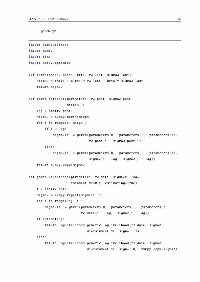
ANNEX A. Code Listings 76
garch.py:
import loglikelihood
import numpy
import time
import scipy.optimize
def garch(omega, alpha, beta, r2_last, sigma2_last):
sigma2 = omega + alpha ∗ r2_last + beta ∗ sigma2_lastreturn sigma2
def garch_forecast(parameters , r2_past, sigma2_past ,
steps=1):
lag = len(r2_past)
sigma2 = numpy.zeros(steps)
for i in range(0, steps):
if i < lag:
sigma2[i] = garch(parameters[0], parameters[1], parameters[2],
r2_past[i], sigma2_past[i])
else:
sigma2[i] = garch(parameters[0], parameters[1], parameters[2],
sigma2[i − lag], sigma2[i − lag])return numpy.copy(sigma2)
def garch_likelihood(parameters , r2_data, sigma20, lag=1,
tstudent_df=0.0, estimating=True):
t = len(r2_data)
sigma2 = numpy.repeat(sigma20, t)
for i in range(lag, t):
sigma2[i] = garch(parameters[0], parameters[1], parameters[2],
r2_data[i − lag], sigma2[i − lag])if estimating:
return loglikelihood.generic_loglikelihood(r2_data, sigma2,
df=tstudent_df , sign=−1.0)else:
return loglikelihood.generic_loglikelihood(r2_data, sigma2,
df=tstudent_df , sign=1.0), numpy.copy(sigma2)
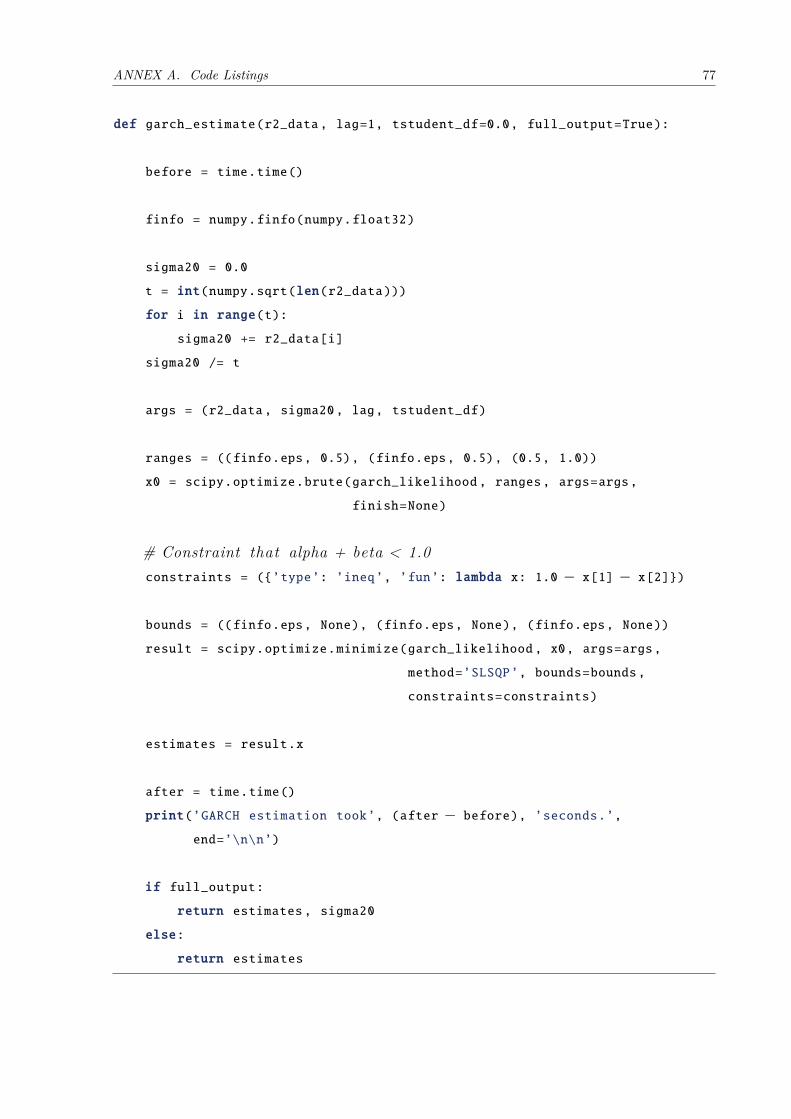
ANNEX A. Code Listings 77
def garch_estimate(r2_data, lag=1, tstudent_df=0.0, full_output=True):
before = time.time()
finfo = numpy.finfo(numpy.float32)
sigma20 = 0.0
t = int(numpy.sqrt(len(r2_data)))
for i in range(t):
sigma20 += r2_data[i]
sigma20 /= t
args = (r2_data, sigma20, lag, tstudent_df)
ranges = ((finfo.eps, 0.5), (finfo.eps, 0.5), (0.5, 1.0))
x0 = scipy.optimize.brute(garch_likelihood , ranges, args=args,
finish=None)
# Constraint that alpha + beta < 1.0constraints = ({’type’: ’ineq’, ’fun’: lambda x: 1.0 − x[1] − x[2]})
bounds = ((finfo.eps, None), (finfo.eps, None), (finfo.eps, None))
result = scipy.optimize.minimize(garch_likelihood , x0, args=args,
method=’SLSQP’, bounds=bounds,
constraints=constraints)
estimates = result.x
after = time.time()
print(’GARCH estimation took’, (after − before), ’seconds.’,end=’\n\n’)
if full_output:
return estimates , sigma20
else:
return estimates