Rethinking Machine Learning in the 21st Century: …mahadeva/Site/IBM Research April 21 2014...

Rethinking Machine Learning in the 21st Century: From

Optimization to EquilibrationSridhar Mahadevan!

Autonomous Learning Laboratory!School of Computer Science!

University of Massachusetts, Amherst

Part I: Motivation

Autonomous Learning Laboratory (formerly Adaptive Networks Laboratory, pre 2001)

(Total: 29 graduated PhD students, 5 postdocs, 4 MS students, 3 undergrads)

Lab Directors

Thomas Boucher

CJ Carey

Bruno Castro da Silva

William Dabney

Stefan Dernbach

Kimberly Ferguson

Ian Gemp

Stephen Giguere

Thomas Helmuth

Nicholas Jacek

Bo Liu

Clemens Rosenbaum

Andrew Stout

Philip Thomas

Chris Vigorito

Current PhD Students

Barto

Notable ALL/ANW Alumni (Total: 29 graduated PhD students, 5 postdocs, 4

MS students, 3 undergrads)

Michael Jordan (postdoc)

Professor of Statistics, U.C. Berkeley (h-index: 112)

Richard Sutton Professor, U. Alberta

(h-index: 53)

Satinder Singh Professor, U. Michigan

(h-index: 48)

Mohammad Ghavamzadeh Adobe Research

(h-index: 16)

George Konidaris Postdoc, MIT (h-index: 16)

Doina Precup Associate Professor,

McGill (h-index: 28)

Suchi Saria Assistant Professor,

Johns Hopkins Mount Holyoke (PhD: Stanford

(Advisor: Daphne Koller))

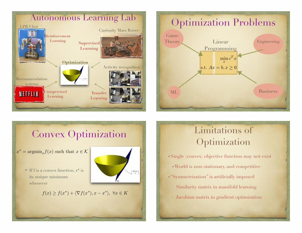
Autonomous Learning Lab

Optimization

Supervised Learning

Reinforcement Learning

Unsupervised Learning

Transfer Learning

LPR UbotCuriosity Mars Rover

Activity recognition

Recommendation systems

Optimization Problems

Linear Programming

minx

c

T

x

s.t. Ax = b, x � 0

Game Theory Engineering

ML Business

Convex Optimization

If f is a convex function, x* is its unique minimum whenever

f(x) � f(x⇤) + hrf(x⇤), x� x

⇤i, 8x 2 K

x

⇤ = argminx

f(x) such that x 2 K

Limitations of Optimization

•Single (convex) objective function may not exist

•World is non-stationary, and competitive

•“Symmetrization” is artificially imposed

• Similarity matrix in manifold learning

• Jacobian matrix in gradient optimization

The “Invisible Hand” of the Internet

“The Internet is an equilibrium — we just have to identify the game (Scott Shenker)”

!“The Internet was the first computational artifact that

was not created by a single entity, but emerged from the strategic interaction of many (Christos Papadimitriou)”

!!

Adam Smith The Wealth of Nations

1776

Changes at IBM

Brendan Mcdermid/Reuters !

Virginia M. Rometty, IBM’s chief executive, last week announced the

company’s new Watson division, which will have 2,500 employees. “This is a key growth area for IBM,” said Erich Clementi, senior vice president of IBM Global

Technology Services. “We are building out a global footprint.” In addition to selling raw computing and data storage capabilities, he said, IBM plans to offer

over 150 software and software development products in its cloud. Among the products is Watson, an advanced cognitive computing

framework. Last week, IBM’s chief executive, Virginia Rometty, announced a new business group

inside IBM for Watson.

IBM Plans Big Spending for the Cloud By QUENTIN HARDY JANUARY 16, 2014,

NY Times !

IBM is moving rapidly on its plans to spend heavily on cloud computing. It expects to spend $1.2 billion this year on

increasing the number and quality of computing centers it has worldwide.

!The move reflects the speed at which the business of renting a

lot of computing power via the Internet is replacing the conventional business of selling mainframe computers,

computer servers, and associated hardware and software. Champions of cloud computing cite both lower costs and faster

deployment as the reasons for the shift. !!!!

http://www.mghpcc.org/http://www.bu.edu/

http://www.harvard.edu/

http://web.mit.edu/

http://www.massachusetts.edu/http://www.northeastern.edu/http://www.cisco.com/

http://www.emc.com/

“Netflix” Cache Problem (Dernbach, Kurose, Mahadevan, Technicolor)

✓⌘◆⇣✓⌘◆⇣✓⌘◆⇣

✓⌘◆⇣✓⌘◆⇣✓⌘◆⇣

✓⌘◆⇣✓⌘◆⇣✓⌘◆⇣

?

?

@@@@@R

@@@@@R

PPPPPPPPPPPPPPq

PPPPPPPPPPPPPPq

?

?

HHHHHHHHHj

HHHHHHHHHj

��

��

��

��

?

?

��⇡

��⇡

⇣⇣⇣⇣⇣⇣⇣⇣⇣⇣⇣⇣⇣⇣)

⇣⇣⇣⇣⇣⇣⇣⇣⇣⇣⇣⇣⇣⇣)

· · ·

· · ·

· · ·

1

1

1

ok· · ·

nj· · ·

mi· · ·

Network Providers

Demand Markets

Service Providers

Figure 1: The Network Structure of the Cournot-Nash-Bertrand Modelfor a Service-Oriented Internet

Professor Anna Nagurney Network Economics and the Internet

Cournot-Nash game

Bertrand game

Next Generation Internet Model [Nagurney et al., 2014] Multiple data sources on Mars Curiosity Rover

Rock Abrasion Tool

Miniature Thermal Emission SpectrometerMoessbauer Spectrometer

Alpha Particle X-ray Spectrometer

Microscopic Imager How to handle competition across across instruments and scientists?

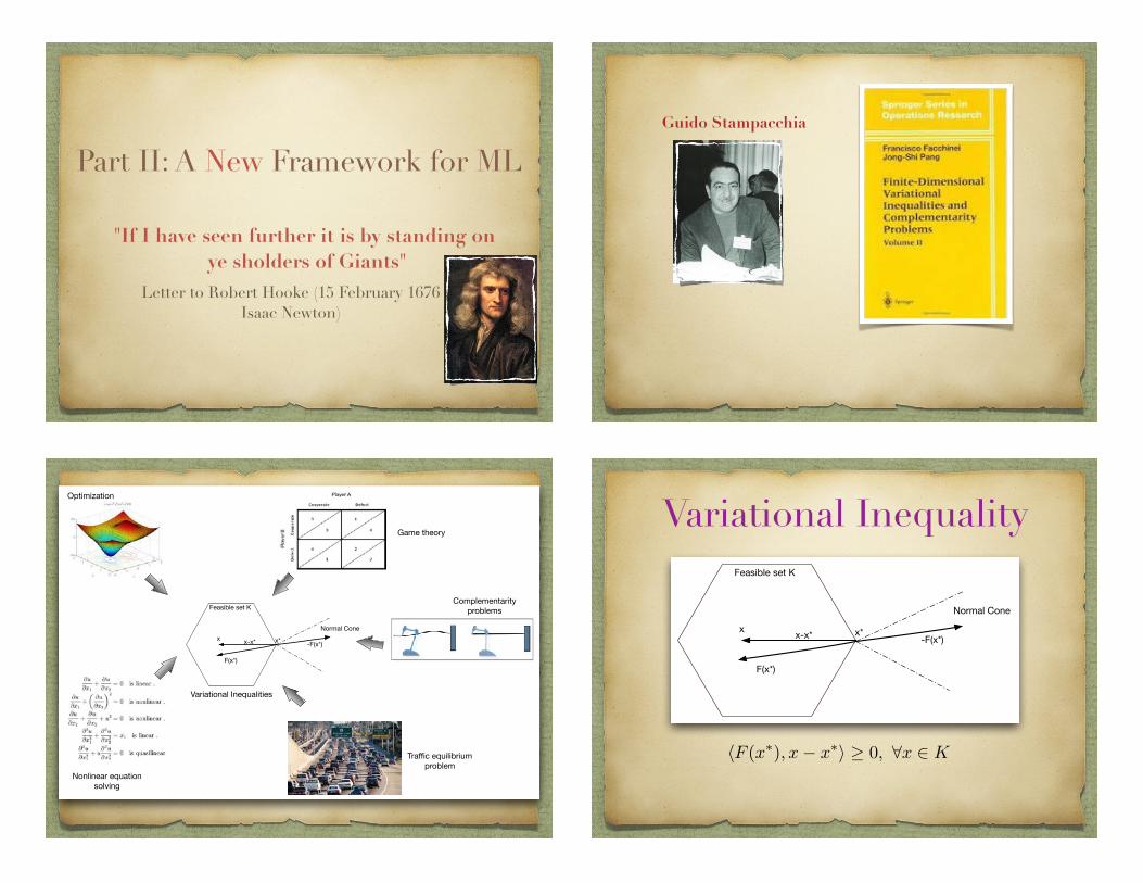
Part II: A New Framework for ML

"If I have seen further it is by standing on ye sholders of Giants"

Letter to Robert Hooke (15 February 1676 Isaac Newton)

Guido Stampacchia

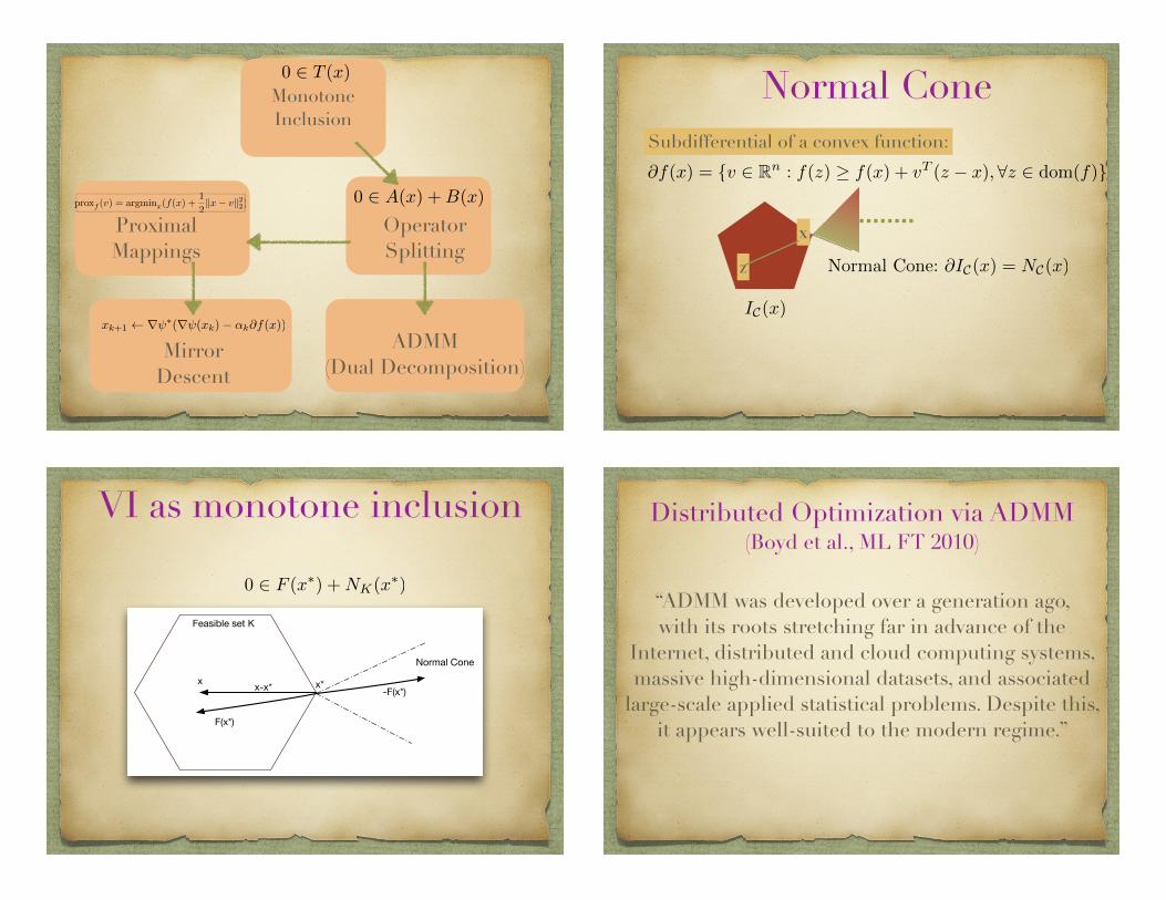
Normal Cone

-F(x*)

F(x*)

x*x x-x*

Feasible set K

Optimization

Game theory

Nonlinear equationsolving

Complementarityproblems

Variational Inequalities

Traffic equilibriumproblem

Variational Inequality

Normal Cone

-F(x*)

F(x*)

x*x x-x*

Feasible set K

hF (x⇤), x� x

⇤i � 0, 8x 2 K

Convex Optimization => VI

f(x) � f(x⇤) + hrf(x⇤), x� x

⇤i, 8x 2 K

Optimization => VI

Suppose x

⇤= argmin

x2Kf(x)

where f is di↵erentiable

Then x

⇤solves the VI

hrf(x

⇤), x� x

⇤i � 0. 8x 2 K

Proof: Define �(t) = f(x

⇤+ t(x� x

⇤)

Since �(0) achieves the minimum

�

0(0) = hrf(x

⇤), x� x

⇤i � 0

When VI => optimization?

Given V I(F,K), define rF (x) =

2

64

@F1@x1

. . .

@F1@xn

... . . .

...@Fn@x1

. . .

@Fn@xn

3

75

When rF is symmetric and positive semi-definite

VI(F,K) can be reduced to an optimization problem,

Optimization vs VIs

Property Optimization VI

Mapping (Strong) Convexity(Strong)

Monotonicity

Jacobian Positive definite and symmetric

Asymmetric

Objective function Single fixed Multiple or none

Traffic Network Equilibrium (Dafermos, Nagurney)

Link travel cost functions

Ca(Fa) = 10*Fa

Cb(Fb) = Fb + 50

Cc(Fc) = Fc + 50

Cd(Fd) = 10 Fd

Travel demand D14 = 6

Find equilibrium flows

1

3

4

a b

c d

2

Traffic Network Equilibrium (Dafermos, Nagurney)

1

3

4

a b

c d

2

Flows at equilibrium

Fa = Fb = 3

Fc = Fd = 3

Ca = 30, Cb = 53

Cc = 53, Cd = 30

Path costs = 83

Nash equilibrium

e

Travel cost = 92!

Part II: Algorithms

Composite Objective Functions from recent ALL Research

shown in [24] that the d columns of the embeddingmatrix F in equation (7) are equal to the d smallestnon-zero eigenvectors, the eigenvectors associated withthe smallest non-zero eigenvalues, of the Laplacian L

in the generalized eigenvalue problem LF = �DF .

3 Low Rank Embedding

Low rank embedding (LRE) is a variation on locallylinear embedding (LLE) [17] that uses low rank ma-trix approximations instead of LLE’s nearest neighborapproach to calculate a reconstruction coe�cients ma-trix [12]. LRE is a two part algorithm. Given a dataset X, LRE begins by calculating the reconstructioncoe�cients matrix R by minimizing the loss function,

minR

1

2||X �XR||2F + �||R||⇤, (8)

where ||X||⇤ =P

i �i(X) for singular values �i is thespectral norm. In [5] it was shown that the spectralnorm is a convex relaxation of the rank minimizationproblem, and so the solution XR is a low rank ap-proximation of the original data matrix X. To solveequation (8), the alternating direction method of mul-tipliers (ADMM) [3] is used.

The generic ADMM optimization problem considersconvex functions f and g and minimizes the con-strained equation

min f(x) + g(z) subject to Ax+Bz = c. (9)

In the case of LRE, f is the Frobenius norm mini-mization and g is the spectral norm minimization inequation (8). To apply ADMM we introduce a newvariable Z and equation (8) becomes

minZ,R

1

2||X �XR||2F + �||Z||⇤, s.t. R = Z. (10)

To solve the constrained optimization problem of equa-tion (10), the augmented Lagrangian function L is in-troduced,

L(Z,R,L) =1

2||X �XR||2F + �||Z||⇤

+ tr(L(R� Z)>) +�

2||R� Z||2F , (11)

where � is the penalty parameter that controls the con-vergence of the ADMM algorithm and � is the param-eter that controls the penalty on the rank.

The ADMM algorithm consists of three steps. In thefirst two steps, Z and R are updated by minimizingL, and in the last step, L is updated with the errorviolating the R = Z constraint. When updating Z inpractice, singular value thresholding (SVT) [4] is used

to minimize the spectral norm. Algorithm 2 detailsthe calculation to solve equation (11).

The second step of LRE preserves point-wise local lin-earity, holding the reconstruction matrix R fixed whileminimizing the reconstruction loss in the embeddedspace,

minF (X)

1

2||F (X) � F

(X)R||2F s.t. (F (X))>F (X) = I, (12)

where F (X) is the embedding ofX and I is the identitymatrix. The constraint (F (X))>F (X) = I ensures thatit is a well-posed problem. In [18] it was shown thatequation (12) can be minimized by calculating the d

smallest non-zero eigenvectors of the Gram matrix (I�R)>(I �R).

4 Low Rank Alignment

Low rank alignment (LRA) is a novel manifold align-ment algorithm that uses a variant of LRE to em-bed the data sets to a joint manifold space, unlikeprevious non-linear manifold alignment methods thathave been based on Laplacian eigenmaps [2, 23, 24]and Isomap [20, 25]. These methods rely on nearest-neighbor graph construction algorithms, and are thusprone to creating spurious inter-manifold connectionswhen mixtures of manifolds are present. These so-called short-circuit connections are most commonlyfound at junction points between manifolds. In con-trast, LRA is able to avoid this problem, successfullyaligning data sets drawn from a mixture of manifolds.

LRA di↵ers from other manifold alignment algorithmsin several key aspects.

Where some previous algorithms embed data using theeigenvectors of the graph Laplacian to preserve bothinter-set correspondences and intra-set local geome-try, LRA minimizes the eigenvectors of the sum of theLaplacian and the local Gram matrix to preserve theinter-set correspondences and the intra-set local linear-ity. Moreover, previous manifold alignment algorithmsrequire a reliable measure of similarity between near-est neighbor samples, whereas LRA relies on the linearweights used in sample reconstruction. Lastly, becauseLRA uses the global property of rank to calculate itsreconstruction matrix, it can better discern the globalstructure of mixing manifolds [12].

We now describe the low rank alignment algorithmfor two data sets. It begins with the same setup asmanifold alignment: two data sets X and Y are given,along with the correspondence matrix C

(X,Y ) describ-ing inter-set correspondences (defined identically toW

(X,Y ) in equation (1)). The goal of LRA is to cal-culate a set of embeddings F

(X) and F

(Y ) to a joint,

Low-rank embedding:

minx2X

f(x) + g(x) : min�2Rk

kX� � yk22 + �k�k1Lasso:

RO-TD:

“Sparse” Supervised learning

“Saddle Point” Reinforcement Learning

Unsupervised learning

min

x

kAx� bkm

+ h(x) = min

x

max

kykn1y

T

(Ax� b) + h(x)

Proximal Mappings

Operator Splitting

Mirror Descent

ADMM (Dual Decomposition)

Monotone Inclusion

0 2 T (x)

0 2 A(x) +B(x)

xk+1 r ⇤(r (xk)� ↵k@f(x))

prox

f

(v) = argmin

x

(f(x) +

1

2

kx� vk22)

Normal Cone

@f(x) = {v 2 Rn: f(z) � f(x) + v

T(z � x), 8z 2 dom(f)}

IC(x)

x

Normal Cone: @IC(x) = NC(x)z

Subdifferential of a convex function:

VI as monotone inclusion

Normal Cone

-F(x*)

F(x*)

x*x x-x*

Feasible set K

0 2 F (x⇤) +NK(x⇤)

Distributed Optimization via ADMM (Boyd et al., ML FT 2010)

“ADMM was developed over a generation ago, with its roots stretching far in advance of the

Internet, distributed and cloud computing systems, massive high-dimensional datasets, and associated

large-scale applied statistical problems. Despite this, it appears well-suited to the modern regime.”

Convex Feasibility Problem10 Proximal Splitting Methods in Signal Processing 17

C

D

x0

x1x2 x3 x∞

y1y2 y3

x4

y4C

D

y0 x∞

x0

x2 x3

x1

Fig. 10.3 Forward-backward versus Douglas–Rachford: As in Example 10.12, letC and D be twoclosed convex sets and consider the problem (10.30) of finding a point x∞ inC at minimum distancefrom D. Let us set f1 = ιC and f2 = d2D/2. Top: The forward–backward algorithm with γn ≡ 1 andλn≡ 1. As seen in Example 10.12, it assumes the form of the alternating projection method (10.31).Bottom: The Douglas–Rachford algorithm with γ = 1 and λn ≡ 1. Table 10.1.xii yields prox f1 = PCand Table 10.1.vi yields prox f2 : x "→ (x+PDx)/2. Therefore the updating rule in Algorithm 10.15reduces to xn = (yn+PDyn)/2 and yn+1 = PC(2xn− yn)+ yn− xn = PC(PDyn)+ yn− xn.

Proximal splitting methods in signal processing Combetti and Pesquet

Operator Splitting

xk+1 (I + �A)�1(I � �B)xk

Manifold Learning

Single Manifold (LLE, ISOMAP, Diffusion Maps,

Laplacian Eigenmaps)

Mixture of Manifolds (Low-rank embedding)

Manifold)Warping (Vu,)Carey,)and)Mahadevan,)AAAI)2012)

• Combine)dynamic)time)warping)and)manifold)alignment)using)alternating)projections)

• Minimize)the)loss)function)to)preserve)local)geometry)and)correspondences

• CMU Multimodal activity dataset • Measure human activity while cooking • 26 subjects • 5 different recipes

Manifold Alignment over time

MARS Curiosity Rover

Boucher, Carey, Darby, Mahadevan, 2014

Mineral Spectra

Curiosity zapping a rock with a laser

Low-Rank Alignment





minR

1

2||X �XR||2F + �||R||⇤, (8)

where ||X||⇤ =P





minZ,R

1

2||X �XR||2F + �||Z||⇤, s.t. R = Z. (10)


L(Z,R,L) =1

2||X �XR||2F + �||Z||⇤

+ tr(L(R� Z)>) +�

2||R� Z||2F , (11)





minF (X)

1

2||F (X) � F

(X)R||2F s.t. (F (X))>F (X) = I, (12)










(X) and F

(Y ) to a joint,

Step 1: Compute Reconstructions





minR

1

2||X �XR||2F + �||R||⇤, (8)

where ||X||⇤ =P





minZ,R

1

2||X �XR||2F + �||Z||⇤, s.t. R = Z. (10)


L(Z,R,L) =1

2||X �XR||2F + �||Z||⇤

+ tr(L(R� Z)>) +�

2||R� Z||2F , (11)





minF (X)

1

2||F (X) � F

(X)R||2F s.t. (F (X))>F (X) = I, (12)










(X) and F

(Y ) to a joint,

Step 2: Compute Low-Dimensional

Embeddings

(ADMM)

Eigen Decomposition

Experimental Results

Martian Spectroscopy EU Parallel Corpus English-German

Boucher, Carey, Darby, Mahadevan, 2014

LRA Cross-lingual AlignmentAstronomy

Optimization in High-Dimensions

Dual

Primal

Mirror!Descent!

(Nemirovski and Yudin)

argminx�Xf(x)

Legendre!Transform

[Thomas, Dabney, Mahadevan, Giguerre, NIPS 2013]

Natural!Gradient!Descent!(Amari)

xk+1 r ⇤k(r (xk)� ↵k@f(xk)) xk+1 xk � ↵kG

�1k rf(xk)

Mirror Descent = Natural Gradient![Thomas, Dabney, Mahadevan, Giguerre, NIPS 2013]

4 Mirror Descent

Mirror descent algorithms form a class of highly scalable online gradient methods that are usefulin constrained minimization of non-smooth functions [17, 18]. They have recently been applied tovalue function approximation and basis adaptation for reinforcement learning [19, 20]. The mirrordescent update is

x

k+1 = r ⇤k

�r

k

(x

k

)� ↵

k

rf(x

k

)

�, (1)

where k

: Rn ! R is a continuously differentiable and strongly convex function called the proxi-mal function, and where the conjugate of

k

is ⇤k

(y) , max

x2Rn {x|y �

k

(x)}, for any y 2 Rn.Different choices of

k

result in different mirror descent algorithms. A common choice for a fixed

k

= , 8k, is the p-norm [20], and a common adaptive k

is the Mahalanobis norm with a dynamiccovariance matrix [15].

Intuitively, the distance metric for the space that xk

resides in is not necessarily the same as that ofthe space that rf(x

k

) resides in. This suggests that it may not be appropriate to directly add x

k

and �↵k

rf(x

k

) in the gradient descent update. To correct this, mirror descent moves xk

into thespace of gradients (the dual space) with r

k

(x

k

) before performing the gradient update. It takesthe result of this step in gradient space and returns it to the space of x

k

(the primal space) with r ⇤k

.Different choices of

k

amount to different assumptions about the relationship between the primaland dual spaces at x

k

.

5 Equivalence of Natural Gradient Descent and Mirror Descent

Theorem 5.1. The natural gradient descent update at step k with metric tensor Gk

, G(x

k

):

x

k+1 = x

k

� ↵

k

G

�1k

rf(x

k

), (2)is equivalent to (1), the mirror descent update at step k, with

k

(x) = (

1/2)x|

G

k

x.

Proof. First, notice that r k

(x) = G

k

x. Next, we derive a closed-form for ⇤k

:

⇤k

(y) = max

x2Rn

⇢x

|y � 1

2

x

|G

k

x

�. (3)

Since the function being maximized on the right hand side is strictly concave, the x that maximizesit is its critical point. Solving for this critical point, we get x = G

�1k

y. Substituting this into (3), wefind that ⇤

k

(y) = (

1/2)y|G�1

k

y. Hence, r ⇤k

(y) = G

�1k

y. Inserting the definitions of r k

(x) andr ⇤

k

(y) into (1), we find that the mirror descent update isx

k+1 =G

�1k

(G

k

x

k

� ↵

k

rf(x

k

)) = x

k

� ↵

k

G

�1k

rf(x

k

),

which is identical to (2). ⌅Although researchers often use

k

that are norms like the p-norm and Mahalanobis norm, noticethat the

k

that results in natural gradient descent is not a norm. Also, since Gk

depends on k, k

isan adaptive proximal function [15].

6 Projected Natural Gradients

When x is constrained to some set, X , k

in mirror descent is augmented with the indicator functionI

X

, where I

X

(x) = 0 if x 2 X , and +1 otherwise. The k

that was shown to generate anupdate equivalent to the natural gradient descent update, with the added constraint that x 2 X , is

k

(x) = (

1/2)x|

G

k

x+ I

X

(x). Hereafter, any references to k

refer to this augmented version.

For this proximal function, the subdifferential of k

(x) is r k

(x) = G

k

(x) +

ˆ

N

X

(x) = (G

k

+

ˆ

N

X

)(x), where ˆ

N

X

(x) , @I

X

(x) and, in the middle term, Gk

and ˆ

N

X

are relations and + denotesMinkowski addition.1 ˆ

N

X

(x) is the normal cone of X at x if x 2 X and ; otherwise [21].r ⇤

k

(y) = (G

k

+

ˆ

N

X

)

�1(y). (4)

1Later, we abuse notation and switch freely between treating Gk as a matrix and a relation. When it is amatrix, Gkx denotes matrix-vector multiplication that produces a vector. When it is a relation, Gk(x) producesthe singleton {Gkx}.

3

4 Mirror Descent

Mirror descent algorithms form a class of highly scalable online gradient methods that are usefulin constrained minimization of non-smooth functions [17, 18]. They have recently been applied tovalue function approximation and basis adaptation for reinforcement learning [19, 20]. The mirrordescent update is

x

k+1 = r ⇤k

�r

k

(x

k

)� ↵

k

rf(x

k

)

�, (1)

where k

: Rn ! R is a continuously differentiable and strongly convex function called the proxi-mal function, and where the conjugate of

k

is ⇤k

(y) , max

x2Rn {x|y �

k

(x)}, for any y 2 Rn.Different choices of

k

result in different mirror descent algorithms. A common choice for a fixed

k

= , 8k, is the p-norm [20], and a common adaptive k

is the Mahalanobis norm with a dynamiccovariance matrix [15].

Intuitively, the distance metric for the space that xk

resides in is not necessarily the same as that ofthe space that rf(x

k

) resides in. This suggests that it may not be appropriate to directly add x

k

and �↵k

rf(x

k

) in the gradient descent update. To correct this, mirror descent moves xk

into thespace of gradients (the dual space) with r

k

(x

k

) before performing the gradient update. It takesthe result of this step in gradient space and returns it to the space of x

k

(the primal space) with r ⇤k

.Different choices of

k

amount to different assumptions about the relationship between the primaland dual spaces at x

k

.

5 Equivalence of Natural Gradient Descent and Mirror Descent

Theorem 5.1. The natural gradient descent update at step k with metric tensor Gk

, G(x

k

):

x

k+1 = x

k

� ↵

k

G

�1k

rf(x

k

), (2)is equivalent to (1), the mirror descent update at step k, with

k

(x) = (

1/2)x|

G

k

x.

Proof. First, notice that r k

(x) = G

k

x. Next, we derive a closed-form for ⇤k

:

⇤k

(y) = max

x2Rn

⇢x

|y � 1

2

x

|G

k

x

�. (3)

Since the function being maximized on the right hand side is strictly concave, the x that maximizesit is its critical point. Solving for this critical point, we get x = G

�1k

y. Substituting this into (3), wefind that ⇤

k

(y) = (

1/2)y|G�1

k

y. Hence, r ⇤k

(y) = G

�1k

y. Inserting the definitions of r k

(x) andr ⇤

k

(y) into (1), we find that the mirror descent update isx

k+1 =G

�1k

(G

k

x

k

� ↵

k

rf(x

k

)) = x

k

� ↵

k

G

�1k

rf(x

k

),

which is identical to (2). ⌅Although researchers often use

k

that are norms like the p-norm and Mahalanobis norm, noticethat the

k

that results in natural gradient descent is not a norm. Also, since Gk

depends on k, k

isan adaptive proximal function [15].

6 Projected Natural Gradients

When x is constrained to some set, X , k

in mirror descent is augmented with the indicator functionI

X

, where I

X

(x) = 0 if x 2 X , and +1 otherwise. The k

that was shown to generate anupdate equivalent to the natural gradient descent update, with the added constraint that x 2 X , is

k

(x) = (

1/2)x|

G

k

x+ I

X

(x). Hereafter, any references to k

refer to this augmented version.

For this proximal function, the subdifferential of k

(x) is r k

(x) = G

k

(x) +

ˆ

N

X

(x) = (G

k

+

ˆ

N

X

)(x), where ˆ

N

X

(x) , @I

X

(x) and, in the middle term, Gk

and ˆ

N

X

are relations and + denotesMinkowski addition.1 ˆ

N

X

(x) is the normal cone of X at x if x 2 X and ; otherwise [21].r ⇤

k

(y) = (G

k

+

ˆ

N

X

)

�1(y). (4)

1Later, we abuse notation and switch freely between treating Gk as a matrix and a relation. When it is amatrix, Gkx denotes matrix-vector multiplication that produces a vector. When it is a relation, Gk(x) producesthe singleton {Gkx}.

3

Fixed Point Formulation

Let ΠK be the projection onto convex set K

Then x* solves VI(F,K) if and only if x* is the fixed point of the mapping given by

x* = ΠK(x* - γF(x*))

Normal Cone

-F(x*)

F(x*)

x*x x-x*

Feasible set K

Projection Algorithmhow to adapt step sizes automatically in Section 3.3. In Section 3.4, we present a detailed study compar-ing our proposed non-Euclidean RK methods with previous methods. In Section 3.5, we discuss scalingour approach using Monte-Carlo methods for solving VIs, and by exploiting decompositional properties ofpartitionable VIs.

3.1 Projection-Based Algorithms for VIs

The basic projection-based method (Algorithm 1) for solving VIs is based on Theorem 4 introduced earlier.

Algorithm 1 The Basic Projection Algorithm for solving VIs.INPUT: Given VI(F,K), and a symmetric positive definite matrix D.

1: Set k = 0 and x

k

2 K.2: repeat3: Set x

k+1 ⇧

K,D

(x

k

�D

�1F (x

k

)).4: Set k k + 1.5: until x

k

= ⇧

K,D

(x

k

�D

�1F (x

k

)).6: Return x

k

Here, ⇧

K,D

is the projector onto convex set K with respect to the natural norm induced by D, wherekxk2

D

= hx, Dxi. It can be shown that the basic projection algorithm solves any V I(F, K) for which themapping F is strongly monotone 4 and Lipschitz.5A simple strategy is to set D = ↵I, where ↵ >

L

2

2µ

, and L

is the Lipschitz smoothness constant, and µ is the strong monotonicity constant. The basic projection-basedalgorithm has two critical limitations: it requires that the mapping F be strongly monotone. If, for example, F

is the gradient map of a continuously differentiable function, strong monotonicity implies the function mustbe strongly convex. Second, setting the parameter ↵ requires knowing the Lipschitz smoothness L and thestrong monotonicity parameter µ. The extragradient method of Korpolevich [22] addresses some of theseconcerns, and is defined as Algorithm 2 below.

Algorithm 2 The Extragradient Algorithm for solving VIs.INPUT: Given VI(F,K), and a scalar ↵.

1: Set k = 0 and x

k

2 K.2: repeat3: Set y

k

⇧

K

(x

k

� ↵F (x

k

)).4: Set x

k+1 ⇧

K

(x

k

� ↵F (y

k

)).5: Set k k + 1.6: until x

k

= ⇧

K

(x

k

� ↵F (x

k

)).7: Return x

k

Figure 3 shows a simple example where Algorithm 1 fails to converge, but Algorithm 2 does. If the initialpoint x0 is chosen to be on the boundary of X, using Algorithm 1, it stays on it and fails to converge to thesolution of this VI (which is at the origin). If x0 is chosen to be in the interior of K, Algorithm 1 will movetowards the boundary. In contrast, using Algorithm 2, the solution can be found for any starting point. Theextragradient algoriithm derives its name from the property that it requires an “extra gradient” step (step 4in Algorithm 2), unlike the basic projection algorithm given earlier as Algorithm 1. The principal advantageof the extragradient method is that it can be shown to converge under a considerably weaker condition onthe mapping F , which now has to be merely monotonic: hF (x) � F (y), x � yi � 0. The earlier Lipschitzcondition is still necessary for convergence.

The extragradient algorithm has been the topic of much attention in optimization since it was proposed,e.g., see [16, 20, 26, 38, 33, 43]. Khobotov [20] proved that the extragradient method converges underthe weaker requirement of pseudo-monotone mappings, 6 when the learning rate is automatically adjusted

4A mapping F is strongly monotone if hF (x)� F (y), x� yi � µkx� yk22, µ > 0,8x, y 2 K.5A mapping F is Lipschitz if kF (x)� F (y)k2 Lkx� yk2,8x, y 2 K.6A mapping F is pseudo-monotone if hF (y), x� yi � 0 ) hF (x), x� yi � 0, 8x, y 2 K.

4

Monotonicity Properties

hF (x)� F (y), x� yi � µkx� yk22, µ > 0, 8x, y 2 K

Strongly monotone mapping:

Lipschitz mapping:

kF (x)� F (y)k2 Lkx� yk2, 8x, y 2 K

Example: if F is the gradient map of a function f, then strong monotonicity of F implies f is strongly convex

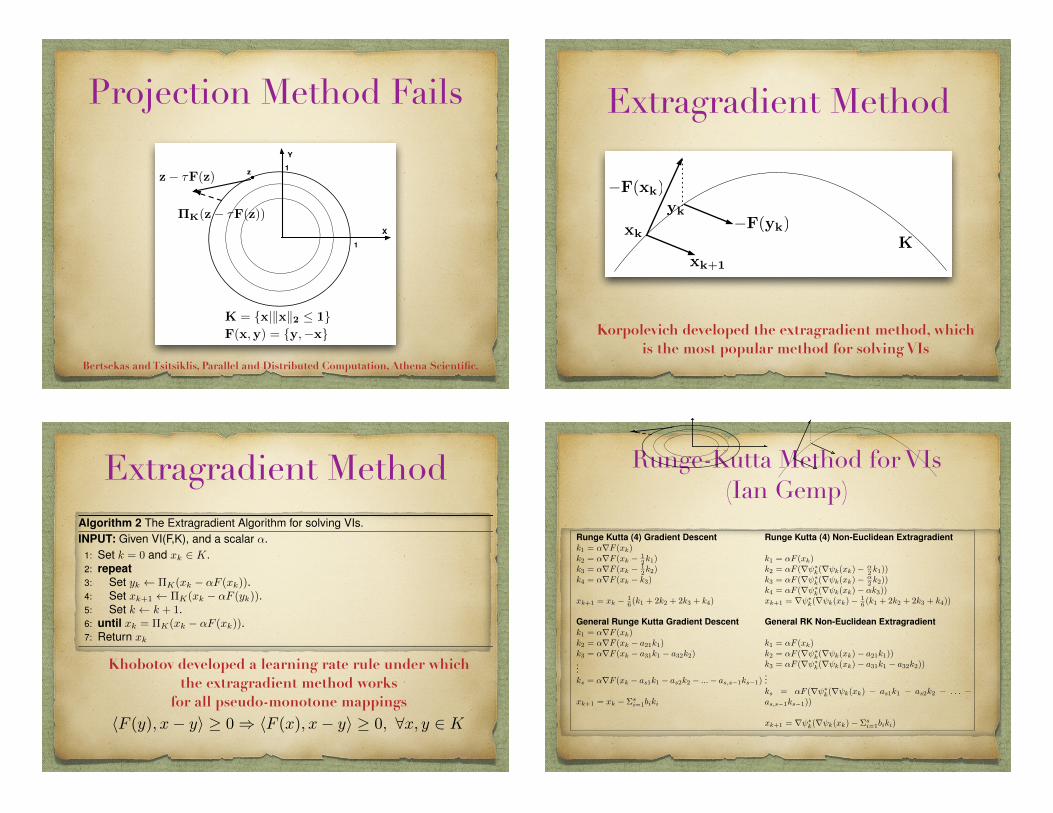
Projection Method FailsY

X

zz� ⌧F(z)

⇧K(z� ⌧F(z))

1

1

K = {x|kxk2 1}F(x,y) = {y,�x}

Bertsekas and Tsitsiklis, Parallel and Distributed Computation, Athena Scientific.

Extragradient Method

xk

�F(xk)

�F(yk)yk

xk+1

K

Korpolevich developed the extragradient method, which is the most popular method for solving VIs

Extragradient Method

how to adapt step sizes automatically in Section 3.3. In Section 3.4, we present a detailed study compar-ing our proposed non-Euclidean RK methods with previous methods. In Section 3.5, we discuss scalingour approach using Monte-Carlo methods for solving VIs, and by exploiting decompositional properties ofpartitionable VIs.

3.1 Projection-Based Algorithms for VIs

The basic projection-based method (Algorithm 1) for solving VIs is based on Theorem 4 introduced earlier.

Algorithm 1 The Basic Projection Algorithm for solving VIs.INPUT: Given VI(F,K), and a symmetric positive definite matrix D.

1: Set k = 0 and x

k

2 K.2: repeat3: Set x

k+1 ⇧

K,D

(x

k

�D

�1F (x

k

)).4: Set k k + 1.5: until x

k

= ⇧

K,D

(x

k

�D

�1F (x

k

)).6: Return x

k

Here, ⇧

K,D

is the projector onto convex set K with respect to the natural norm induced by D, wherekxk2

D

= hx, Dxi. It can be shown that the basic projection algorithm solves any V I(F, K) for which themapping F is strongly monotone 4 and Lipschitz.5A simple strategy is to set D = ↵I, where ↵ >

L

2

2µ

, and L

is the Lipschitz smoothness constant, and µ is the strong monotonicity constant. The basic projection-basedalgorithm has two critical limitations: it requires that the mapping F be strongly monotone. If, for example, F

is the gradient map of a continuously differentiable function, strong monotonicity implies the function mustbe strongly convex. Second, setting the parameter ↵ requires knowing the Lipschitz smoothness L and thestrong monotonicity parameter µ. The extragradient method of Korpolevich [22] addresses some of theseconcerns, and is defined as Algorithm 2 below.

Algorithm 2 The Extragradient Algorithm for solving VIs.INPUT: Given VI(F,K), and a scalar ↵.

1: Set k = 0 and x

k

2 K.2: repeat3: Set y

k

⇧

K

(x

k

� ↵F (x

k

)).4: Set x

k+1 ⇧

K

(x

k

� ↵F (y

k

)).5: Set k k + 1.6: until x

k

= ⇧

K

(x

k

� ↵F (x

k

)).7: Return x

k

Figure 3 shows a simple example where Algorithm 1 fails to converge, but Algorithm 2 does. If the initialpoint x0 is chosen to be on the boundary of X, using Algorithm 1, it stays on it and fails to converge to thesolution of this VI (which is at the origin). If x0 is chosen to be in the interior of K, Algorithm 1 will movetowards the boundary. In contrast, using Algorithm 2, the solution can be found for any starting point. Theextragradient algoriithm derives its name from the property that it requires an “extra gradient” step (step 4in Algorithm 2), unlike the basic projection algorithm given earlier as Algorithm 1. The principal advantageof the extragradient method is that it can be shown to converge under a considerably weaker condition onthe mapping F , which now has to be merely monotonic: hF (x) � F (y), x � yi � 0. The earlier Lipschitzcondition is still necessary for convergence.

The extragradient algorithm has been the topic of much attention in optimization since it was proposed,e.g., see [16, 20, 26, 38, 33, 43]. Khobotov [20] proved that the extragradient method converges underthe weaker requirement of pseudo-monotone mappings, 6 when the learning rate is automatically adjusted

4A mapping F is strongly monotone if hF (x)� F (y), x� yi � µkx� yk22, µ > 0,8x, y 2 K.5A mapping F is Lipschitz if kF (x)� F (y)k2 Lkx� yk2,8x, y 2 K.6A mapping F is pseudo-monotone if hF (y), x� yi � 0 ) hF (x), x� yi � 0, 8x, y 2 K.

4

Khobotov developed a learning rate rule under which the extragradient method works

for all pseudo-monotone mappingshF (y), x� yi � 0 ) hF (x), x� yi � 0, 8x, y 2 K

Runge-Kutta Method for VIs (Ian Gemp)

Y

X

zz � �F(z)

�K(z � �F(z))

1

1

K = {x|kxk2 1}F(x,y) = {y, �x}

xk

�F(xk)

�F(yk)

yk

xk+1

K

Figure 3: Left: This figure illustrates a VI where the basic projection algorithm (Algorithm 1) fails, but theextragradient algorithm (Algorithm 2) succeeds. Right: One iteration of the extradient algorithm.

Runge Kutta (4) Gradient Descentk1 = ↵rF (x

k

)

k2 = ↵rF (x

k

� 12k1)

k3 = ↵rF (x

k

� 12k2)

k4 = ↵rF (x

k

� k3)

x

k+1 = x

k

� 16 (k1 + 2k2 + 2k3 + k4)

General Runge Kutta Gradient Descentk1 = ↵rF (x

k

)

k2 = ↵rF (x

k

� a21k1)

k3 = ↵rF (x

k

� a31k1 � a32k2)

...k

s

= ↵rF (x

k

� a

s1k1 � a

s2k2 � ... � a

s,s�1ks�1)

x

k+1 = x

k

� ⌃

s

i=1bi

k

i

Runge Kutta (4) Non-Euclidean Extragradient

k1 = ↵F (x

k

)

k2 = ↵F (r ⇤k

(r k

(x

k

) � ↵

2 k1))

k3 = ↵F (r ⇤k

(r k

(x

k

) � ↵

2 k2))

k4 = ↵F (r ⇤k

(r k

(x

k

) � ↵k3))

x

k+1 = r ⇤k

(r k

(x

k

) � 16 (k1 + 2k2 + 2k3 + k4))

General RK Non-Euclidean Extragradient

k1 = ↵F (x

k

)

k2 = ↵F (r ⇤k

(r k

(x

k

) � a21k1))

k3 = ↵F (r ⇤k

(r k

(x

k

) � a31k1 � a32k2))

...k

s

= ↵F (r ⇤k

(r k

(x

k

) � a

s1k1 � a

s2k2 � . . . �a

s,s�1ks�1))

x

k+1 = r ⇤k

(r k

(x

k

) � ⌃

s

i=1bi

k

i

)

Figure 4: Left: the proposed Runge Kutta extragradient family of algorithms for solving variational inequal-ities V I(f, K) for the special case of unconstrained function minimization, where f = rF , and K = Rn.Right: the corresponding methods for the general (non-Euclidean) VI problem.

based on a local measure of the Lipschitz constant. Iusem [16] proposed a variant whereby the currentiterate is projected onto a hyperplane separating the current iterate from the final solution, and subsequentlyprojected from the hyperplane onto the feasible set. Solodov and Svaiter [43] proposed another hyperplanemethod, whereby the current iterate is projected onto the intersection of the hyperplane and the feasibleset. Finally, the extragradient method was generalized to the non-Euclidean case by combining it with themirror-descent method [31], resulting in the so-called “mirror-prox” algorithm [18].

3.2 Runge-Kutta Extragradient Algorithms

Figure 4 presents our proposed novel class of algorithms, which generalize the extragradient method usingnumerical methods for solving ordinary differential equations (ODEs), principally the Runge Kutta family[39]. In what follows, we will describe the methods on the left-hand side of Figure 4 for the special caseof unconstrained function minimization in Rn, and subsequently describe the algorithms on the right-handside for the more general non-Euclidean VI setting using Bregman divergences [5], and where the learningrates are automatically adapted. Runge Kutta methods are highly popular methods for solving systems ofcoupled first-order differential equations of the form:

dy

i

dx

= f

i

(x, y1, . . . , yn

), i = 1, . . . , n

5

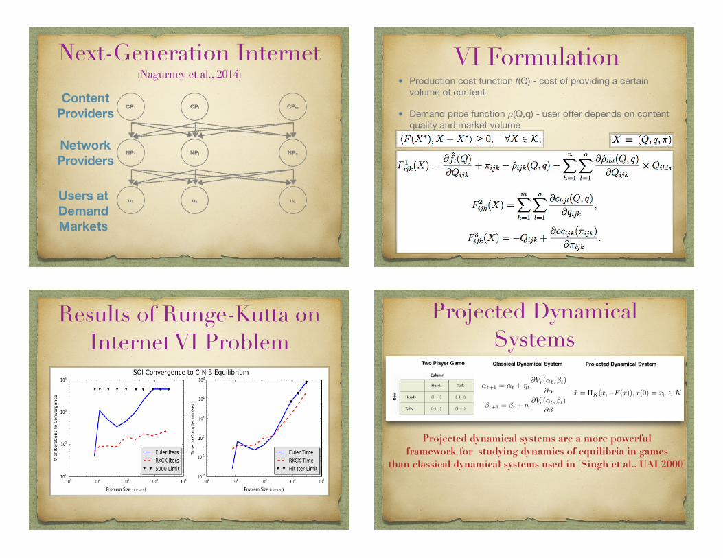
Next-Generation Internet (Nagurney et al., 2014)

CP1 CPi CPm

NP1 NPj NPn

u1 uk uo

Content Providers

Network Providers

Users at Demand Markets

VI FormulationProduction cost function f(Q) - cost of providing a certain volume of content

Demand price function !(Q,q) - user offer depends on content quality and market volume

Results of Runge-Kutta on Internet VI Problem

Projected Dynamical Systems

↵t+1 = ↵t + ⌘t@Vr(↵t,�t)

@↵

�t+1 = �t + ⌘t@Vc(↵t,�t)

@�

x = ⇧K(x,�F (x)), x(0) = x0 2 K

Two Player Game Classical Dynamical System Projected Dynamical System

Projected dynamical systems are a more powerful framework for studying dynamics of equilibria in games

than classical dynamical systems used in [Singh et al., UAI 2000]

PDS Formulation

X* solves the VI iff it is a stationary point of the projected ODE

Lipschitz continuity of F(X) guarantees the existence of a unique solution

Stability of equilibrium is given by the monotonicity of F(X) which can be determined from the positive-definiteness of the Jacobian of F(X)

Fixed Point Problem

Projection Operator

ODE/IVP

Skorokhod Analysis�

x

(t) = ⇧K

(�x

(t),�F (�x

(t))), �

x

(0) = x

F1(x1, x2) = �x2, F2(x1, x2) = 4x1

A

B

C

D

0

Alternating Direction Method of Multipliers

Minimize f(x) + g(x)

Solve 0 2 @f(x) + @g(x)

Choose A(x) = @g(x), B(x) = @f(x)

x

k+ 12= argmin

x

(f(x) +1

2�kx� z

k

k22)

z

k+ 12= 2x

k+ 12� z

k

x

k+1 = argminx

(g(x) +1

2�kx� x

k+ 12k22)

z

k+1 = z

k

+ x

k+1 � x

k+ 12

ADMM is an instance of Douglas Rachford

splitting

ADMM for Cloud Computing

10.4 MapReduce 83

that is, it takes a key-value pair and emits a list of intermediatekey-value pairs. The engine then collects all the values v′

1, . . . ,v′r that

correspond to the same output key k′ (across all Mappers) and passesthem to the Reduce functions, which performs the transformation

(k′, [v′1, . . . ,v

′r]) !→ (k′′,R(v′

1, . . . ,v′r)),

where R is a commutative and associative function. For example, Rcould simply sum v′

i. In Hadoop, Reducers can emit lists of key-valuepairs rather than just a single pair.

Each iteration of ADMM can easily be represented as a MapRe-duce task: The parallel local computations are performed by Maps,and the global aggregation is performed by a Reduce. We will describea simple global consensus implementation to give the general flavorand discuss the details below. Here, we have the Reducer compute

Algorithm 2 An iteration of global consensus ADMM in Hadoop/ MapReduce.

function map(key i, dataset Di)1. Read (xi,ui, z) from HBase table.2. Compute z := proxg,Nρ((1/N)z).3. Update ui := ui + xi − z.4. Update xi := argminx

!fi(x) + (ρ/2)∥x − z + ui∥2

2".

5. Emit (key central, record (xi,ui)).

function reduce(key central, records (x1,u1), . . . ,(xN ,uN ))1. Update z :=

#Ni=1 xi + ui.

2. Emit (key j, record (xj ,uj , z)) to HBase for j = 1, . . . ,N .

z =!N

i=1(xi + ui) rather than z or z because summation is associa-tive while averaging is not. We assume N is known (or, alternatively,the Reducer can compute the sum

!Ni=1 1). We have N Mappers, one

for each subsystem, and each Mapper updates ui and xi using thez from the previous iteration. Each Mapper independently executesthe proximal step to compute z, but this is usually a cheap opera-tion like soft thresholding. It emits an intermediate key-value pair thatessentially serves as a message to the central collector. There is a sin-gle Reducer, playing the role of a central collector, and its incomingvalues are the messages from the Mappers. The updated records are

Boyd et al., ML Fn Trends, 2010

Bregman DivergenceBregman Divergences: Definition

Let ϕ : S → R be a differentiable, strictly convex function of “Legendretype” (S ⊆ Rd)The Bregman Divergence Dϕ : S × relint(S)→ R is defined as

Dϕ(x, y) = ϕ(x)− ϕ(y)− (x− y)T∇ϕ(y)

y

x

Dϕ(x ,y)=x log xy−x+y

h(z)

ϕ(z)=z log z

Relative Entropy (or KL-divergence) is another Bregman divergence

Inderjit S. Dhillon University of Texas at Austin Learning with Bregman Divergences

KL divergence

Bregman ADMMspecifically, given yt and zt, xt+1 can be obtained by solving Lφρ(x, zt,yt) as ADMM does. Inother words, the quadratic penalty term 1

2∥Ax+Bzt−c∥22 in (3) is replaced withBφ(c−Ax,Bzt)in the x update of BADMM. However, we cannot get zt+1 by solving Lφρ(xt+1, z,yt), sinceLφρ(xt+1, z,yt) contains the termBφ(c−Axt+1,Bz)which is not convex in z. Instead, the z updateof BADMM uses Bφ(Bz, c−Axt+1) to replace the quadratic penalty term 1

2∥Axt+1 +Bz− c∥22in (3). It is worth noting that the same Bregman divergence Bφ is used in the x and z updates. Toallow the use of different Bregman divergences, additional Bregman divergences are introduced inthe x and z updates, which give more options for solving them efficiently. Therefore, we formallypropose the following updates for BADMM:

xt+1 = argminx∈X

f(x) + ⟨yt,Ax+Bzt − c⟩+ ρBφ(c−Ax,Bzt) + ρxBϕx(x,xt) , (7)

zt+1 = argminz∈Z

g(z) + ⟨yt,Axt+1 +Bz− c⟩+ ρBφ(Bz, c−Axt+1) + ρzBϕz(z, zt) , (8)

yt+1 = yt + τ(Axt+1 +Bzt+1 − c) . (9)

where ρ > 0, τ > 0, ρx ≥ 0, ρz ≥ 0. Note that three Bregman divergences are used in BADMM. Ifall three of them are quadratic functions, Bregman ADMM reduces to generalized ADMM [8]. Weallow the use of a different step size τ in the dual variable update [8, 21]. The global convergencefor BADMM will be shown in Section 3.

We will discuss some special cases in two scenarios. In scenario 1 where ρx, ρz are zero,BADMM simply replaces the quadratic penalty term in ADMM by a single Bregman divergence.In this scenario, the x and z updates should be solved exactly. In scenario 2 where one or both ofρx, ρz are positive, we can choose different Bregman divergences in the x and z updates so thatthey can be solved inexactly. Compared to scenario 1, scenario 2 usually takes more iterationsto converge but may be less expensive in solving the x and z updates. Since (7) and (8) aresymmetric, the discussion below focuses on the x update, and can be applied for the z update. Asa gentle reminder, the global convergence for BADMM in Section 3 automatically applies for thespecial cases considered here.

2.1 Scenario 1: Exact BADMM UpdateIf ρx = ρz = 0, BADMM simply uses a single Bregman divergence to replace the quadraticpenalty term in ADMM. This scenario is particularly useful when a single Bregman divergence φcan yield efficient algorithms for both the x and z updates.

In a special case, like consensus optimization [4], whenA = −I,B = I, c = 0, (7) becomes

xt+1 = argminx∈X

f(x) + ⟨yt,−x+ zt⟩+ ρBφ(x, zt) . (10)

This special case is similar to Case 2 in Scenario 2. Further, if f is a linear function and X is theunit simplex, we have multiplicative update when using KL divergence. If the z update is also amultiplicative update, we have alternating multiplicative updates. In Section 4, we will show theminimization over doubly stochastic matrices can be cast into this scenario.

4

“There is no known proof of convergence known for ADMM with non-quadratic penalty terms”, Boyd et al., 2010

Wang and Banerji, 2013:

Bauschke et al., 2004:

Therefore, Problem (4) can be viewed as a relaxation of

(7) minimize (x, y) !→ ϕ(x) + ψ(y) + ι∆(x, y) over U × U,

which, in turn, is equivalent to the standard problem

(8) minimize ϕ + ψ over U.

For the sake of illustration, let us consider the case when f = 12∥ · ∥

2, so that U = X andD : (x, y) !→ 1

2∥x− y∥2. If ϕ and ψ are the indicator functions of two nonempty closed convex setsA and B, respectively, then (8) corresponds to the convex feasibility problem of finding a point inA ∩B. When no such point exists, a sensible alternative is to look for a pair (x, y) ∈ A× B suchthat ∥x− y∥ = inf ∥A−B∥. This formulation, which corresponds to (4), was proposed in [21] andhas found many applications in engineering [22, 35, 38]. The algorithm devised in [21] to solve thisjoint best approximation problem is the alternating projections method

(9) fix x0 ∈ X and set (∀n ∈ N) yn = PB(xn) and xn+1 = PA(yn).

More generally, let proxθ : x !→ argminy θ(y)+ 12∥x−y∥2 be the proximity operator [36, 37] associated

with a function θ ∈ Γ0(X). In [1], (9) was extended to the algorithm

(10) fix x0 ∈ X and set (∀n ∈ N) yn = proxψ(xn) and xn+1 = proxϕ(yn)

in order to solve

(11) minimize (x, y) !→ ϕ(x) + ψ(y) + 12∥x− y∥2 over X ×X.

The purpose of this paper is to introduce and analyze a proximal-like method to solve (4) underthe assumptions stated above. The lack of symmetry of D prompts us to consider two single-valuedoperators defined on U , namely

(12) ←−−proxϕ : y !→ argminx∈U

ϕ(x) + D(x, y) and −−→proxψ : x !→ argminy∈U

ψ(y) + D(x, y).

The operators←−−proxϕ and −−→proxψ will be called the left and the right proximity operator, respectively.While left proximity operators have already been used in the literature (see [6] and the referencestherein), the notion of a right proximity operator at this level of generality appears to be new. Wenote that [27, p. 26f] observes (but does not exploit) a superficial similarity between the iterativestep of a multiplicative algorithm and the application of the right proximity operator −−→proxψ in theKullback-Leibler divergence setting (see Example 2.5(ii)), where ψ is assumed to be the sum of acontinuous convex function and the indicator function of the nonnegative orthant in X.

In this paper, we shall provide a detailed analysis of these operators and establish key properties.With these tools in place, we shall be in a position to tackle (4) by alternating minimizations of Λ.We thus obtain the following algorithm

(13) fix x0 ∈ U and set (∀n ∈ N) yn = −−→proxψ(xn) and xn+1 =←−−proxϕ(yn).

3












in order to solve





ψ(y) + D(x, y).




3












in order to solve





ψ(y) + D(x, y).




3

Generalized ADMM Method for Separable VIs

(Tseng, 1988)

hx� x

⇤, R(x⇤)i+ hz � z

⇤, S(z⇤)i � 0,

8(x, z) 2 X ⇥ Z s.t. Ax+Bz = b

Minimize hR(x⇤), xi+ hS(z⇤), zis.t. x 2 X, z 2 Z,Ax+Bz = b

Let N(.|X), N(.|Z) be subdi↵erentials of �(.|X), �(.|Z)

Let p

⇤be the optimal Lagrange multiplier for Ax+Bz = b

Generalized ADMM for Separable VIsKarush Kuhn Tucker conditions imply:

A

Tp

⇤ 2 N(x

⇤|X) +R(x

⇤)

B

Tp

⇤ 2 N(z

⇤|Z) + S(z

⇤)

Ax

⇤+Bz

⇤= b

Define maximal monotone operators

F (x) = R(x) +N(x|X)

G(z) = S(z) +N(z|Z)

Above equations can be rewritten as:

AF�1(AT p⇤) +BG�1

(BT p⇤) = b

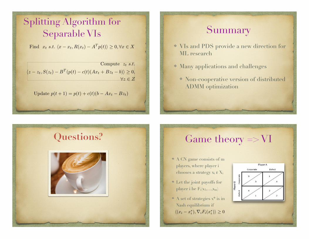
Splitting Algorithm for Separable VIs

Find xt s.t. hx� xt, R(xt)�A

Tp(t)i � 0, 8x 2 X

Compute zt s.t.

hz � zt, S(zt)�B

T(p(t)� c(t)(Axt +Bzt � b)i � 0,

8z 2 Z

Update p(t+ 1) = p(t) + c(t)(b�Axt �Bzt)

SummaryVIs and PDS provide a new direction for ML research

Many applications and challenges

Non-cooperative version of distributed ADMM optimization

Questions? Game theory => VI

A CN game consists of m players, where player i chooses a strategy xi ε Xi

Let the joint payoffs for player i be Fi(x1,…,xm)

A set of strategies x* is in Nash equilibrium if

Proof: Define �(t) = f(x

⇤+ t(x � x

⇤)). Since �(t) is minimized at t = 0, it follows that 0 �

0(0) =

hrf(x

⇤), x � x

⇤i � 0, 8x 2 K, that is x

⇤ solves the VI.

Theorem 3. If f(x) is a convex function, and x

⇤ is the solution of V I(rf, K), then x

⇤ minimizes f .

Proof: Since f is convex, it follows that any tangent lies below the function, that is f(x) � f(x

⇤) +

hrf(x

⇤), x � x

⇤i, 8x 2 K. But, since x

⇤ solves the VI, it follows that f(x

⇤) is a lower bound on the value of

f(x) everywhere, or that x

⇤ minimizes f .A rich class of problems called complementarity problems (CPs) also can be reduced to solving a VI.

When the feasible set K is a cone, meaning that if x 2 K, then ↵x 2 K, ↵ � 0, then the VI becomes a CP.

Definition 2. Given a cone K ⇢ Rn, and a mapping F : K ! Rn, the complementarity problem CP(F,K) isto find an x 2 K such that F (x) 2 K

⇤, the dual cone to K, and hx, F (x)i � 0. 3

A number of special cases of CPs are important. The nonlinear complementarity problem (NCP) is tofind x

⇤ 2 Rn

+ (the non-negative orthant) such that F (x

⇤) � 0 and hF (x

⇤), x

⇤i = 0. The solution to an NCPand the corresponding V I(F,Rn

+) are the same, showing that NCPs reduce to VIs. In an NCP, wheneverthe mapping function F is affine, that is F (x) = Mx+b, where M is an n⇥n matrix, then the correspondingNCP is called a linear complementarity problem (LCP) [27]. Recent work on learning sparse models usingL1 regularization has exploited the fact that the standard LASSO objective [50] of L1 penalized regressioncan be reduced to solving an LCP [21]. This reduction to LCP has been used in recent work on sparsevalue function approximation as well in a method called LCP-TD [17]. A final crucial property of VIs is thatthey can be formulated as finding fixed points.

Theorem 4. The vector x

⇤ is the solution of VI(F,K) if and only if, for any � > 0, x

⇤ is also a fixed point ofthe map x

⇤= ⇧

K

(x

⇤ � �F (x

⇤)), where ⇧

K

is the projector onto convex set K.

In terms of the geometric picture of a VI illustrated in Figure 2. this property means that the solution ofa VI occurs at a vector x

⇤ where the vector field F (x

⇤) induced by F on K is normal to the boundary of K

and directed inwards, so that the projection of x

⇤ � �F (x

⇤) is the vector x

⇤ itself. This property forms thebasis for the projection class of methods that solve for the fixed point.

2.1 Equilibrium Problems in Game Theory

The VI framework provides a mathematically elegant approach to model equilibrium problems in gametheory [35]. A Nash game consists of m players, where player i chooses a strategy x

i

belonging to aclosed convex set X

i

⇢ Rn. After executing the joint action, each player is penalized (or rewarded) by theamount F

i

(x1, . . . , xm

), where F

i

: Rn

i ! R is a continuously differentiable function. A set of strategiesx

⇤= (x

⇤1, . . . , x

⇤m

) 2Q

M

i=1 X

i

is said to be in equilibrium if no player can reduce the incurred penalty (orincrease the incurred reward) by unilaterally deviating from the chosen strategy. If each F

i

is convex on theset X

i

, then the set of strategies x

⇤ is in equilibrium if and only if h(xi

� x

⇤i

), ri

F

i

(x

⇤i

)i � 0. In other words,x

⇤ needs to be a solution of the VI h(x�x

⇤), f(x

⇤)i � 0, where f(x) = (rF1(x), . . . , rF

m

(x)). Nash gamesare closely related to saddle point problems [18, 19, 23]. where we are given a function F : X ⇥ Y ! R,and the objective is to find a solution (x

⇤, y

⇤) 2 X ⇥ Y such that

F (x

⇤, y) F (x

⇤, y

⇤) F (x, y

⇤), 8x 2 X, 8y 2 Y

Here, F is convex in x for each fixed y, and concave in y for each fixed x. Many equilibria problems ineconomics can be modeled using VIs [29]. Bruckner et al. [6] solve the Nash equilibria problem using theextragradient VI method [22], described below as Algorithm 2.

3 Proposed Research: Algorithms

Section 3.1 reviews projection-based algorithms for solving VIs, including the popular extragradient method[22]. In Section 3.2, we introduce a new family of enhanced extragradient methods based on the Runge-Kutta (RK) family of methods for numerical solution of ordinary differential equations (ODEs), and show

3Given a cone K, the dual cone K

⇤ is defined as K

⇤ = {y 2 Rn|hy, xi � 0, 8x 2 K}.

3

Rethinking Machine Learning in the 21st Century: …mahadeva/Site/IBM Research April 21 2014...

Documents

Transcript of Rethinking Machine Learning in the 21st Century: …mahadeva/Site/IBM Research April 21 2014...