Resilient Localization for Sensor Networks

in Outdoor Environments

YoungMin Kwon, Kirill Mechitov, Sameer Sundresh, Wooyoung Kim and Gul AghaDepartment of Computer Science

University of Illinois at Urbana-Champaign201 N. Goodwin Ave., Urbana, IL 61801, USA

ykwon4,mechitov,sundresh,wooyoung,agha@cs.uiuc.edu

Abstract

A process which computes the physical locations of nodes in a wireless sensor network iscalled localization. Self-localization is critical for large-scale sensor networks because manualor assisted localization is often impractical due to time requirements, economic constraints orinherent limitations of deployment scenarios. We have developed a service for reliably local-izing wireless sensor networks in environments conducive to ranging errors by using a customhardware-software solution for acoustic ranging and a family of self-localization algorithms. Theranging solution improves on previous work, extending the practical measurement range three-fold (20–30m) while maintaining a distance-invariant median measurement error of about 1% ofmaximum range (33cm). The localization scheme is based on least squares scaling with soft con-straints. Evaluation using ranging results obtained from sensor network field experiments showsthat the localization scheme is resilient against large-magnitude ranging errors and sparse rangemeasurements, both of which are common in large-scale outdoor sensor network deployments.

1 Introduction

Localization is the process which assigns location information to the nodes of a wireless sensornetwork (WSN). This is a fundamental middleware service, since many WSN applications assumethe availability of sensor location information. For example, knowledge of the positions of indi-vidual sensor nodes is essential for intrusion detection and target tracking applications. Similarly,geographic routing relies on node locations to forwardi packets, obviating the need for large routingtables. In general, self-localization is critical for deployment of large-scale sensor networks, becausemanual surveying and entry of node coordinates is often impractical, and equipping each node witha specialized positioning device such as a GPS receiver is usually too costly or does not providesufficient accuracy.

A number of algorithms have been proposed for self-localization of sensor networks. Thesealgorithms may be characterized as range-based or range-free, depending, respectively, on whetheror not they require distance measurements between nodes. Unfortunately, most of the proposedschemes have only been studied under idealized conditions such as isotropic networks, high nodedensity, or very high precision ranging. Since these assumptions are generally very difficult toguarantee in large-scale outdoor sensor network deployments, the real-world accuracy and reliabilityof these schemes is unclear.

In order to provide a reliable self-localization service to use in environments conducive to rangingerrors, we have developed a custom hardware-software solution for acoustic ranging and a family of

1

localization algorithms which are particularly suitable for medium- to large-scale outdoor wirelesssensor networks. The ranging and localization services have been implemented and evaluated on theMICA2 mote platform [5] over the past three years. This report describes implementation details ofthe fully-functional ranging and localization algorithms. Each service’s description is accompaniedwith experimental evaluation results obtained with actual range measurement data from medium-scale (3000m2) WSN deployments. To further understand performance under different conditions,we have also conducted additional simulation studies of the localization algorithms, with distancemeasurements randomly generated using parameters collected from the experiments.

The ranging service is based on the time-difference-of-arrival (TDoA) method. Specifically, ituses the difference between the arrival times of synchronized radio and acoustic signals to estimatethe distance between two nodes. This technique was chosen because acoustic signals tend to havepredictable isotropic propagation in open environments, and enable reasonably accurate distancemeasurements at significant range. Furthermore, inexpensive speakers and microphones are readilyavailable.

The original sounder-microphone pair of the MICA sensor board yields a detection range of lessthan 3m on grass. In order to increase the reliable acoustic detection range, we have extended theMICA sensor board with a louder speaker. This hardware extension allows sensor nodes to makerange measurements to a sufficient number of neighbors for successful localization even in low-density deployments. To further extend the measurement range and improve reliability, we haveincorporated a number of filtering techniques into the ranging service, including a signal processingalgorithm to better distinguish signals from noise, statistical filtering, and consistency checking.

We have designed a centralized localization algorithm which tolerates sparse measurement data,as well as a distributed variant which enables scalable deployment. Specifically, we have developeda localization scheme based on least squares scaling (LSS) [11], a multidimensional scaling (MDS)technique. MDS is a family of analysis techniques which find a hidden structure underlying theproximity data in a set of inputs. Unlike classical MDS, LSS does not require that distance mea-surements between all pairs of nodes be available. In particular, we have adapted LSS with softconstraints to exploit deployment-specific requirements such as minimum node spacing. Empiricalevaluation based on ranging results obtained from field experiments in real deployments showsthat the localization schemes are robust and resilient not only against sparse range measurements,but also against large-magnitude ranging errors. Such resilience makes the schemes particularlywell-suited for large-scale, sparse sensor networks, such as outdoor deployments.

2 Related Work

The Global Positioning System (GPS) [9] is by far the most popular standard for electronic outdoorlocalization. GPS receivers use the time difference between emission and reception of a signal from asatellite (called pseudo-random code) to calculate the distance to the satellite. At least four satellitesare used to unambiguously locate a position through three-dimensional trilateration. With selectiveavailability1 turned off (as of May 1, 2000) [2], GPS error is in a 95% confidence interval of ±6.3m,a fairly large error magnitude for wireless micro-sensors with limited communication range. Assuch, many GPS-less and hybrid methods have been proposed for wireless sensor networks.

Many hybrid methods employ a two-tiered approach in which a set of anchor nodes is used tolocalize non-anchor nodes. Anchor nodes are assumed to know their own location (e.g., by manualsurvey and entry, careful deployment, or GPS measurements). Sensor nodes estimate their distances

1The US Government’s intentional degradation of the GPS signals available to the general public.

2

to the anchor nodes and apply triangulation or multilateration to determine their locations. Thevariations lie in the methods used to estimate distances to the anchors.

The Cricket location support system [15] uses a combination of active anchors and passiveultrasonic receivers to provide locationing services. This system was proposed for mobile nodesin an indoor environment, though it can also be used with static nodes. The pre-installed activeanchors broadcast their location information over an RF channel together with an ultrasonic pulse.A mobile node uses the TDoA method to estimate the distance to an anchor.

The GPS-less localization proposed in [3] uses a fixed number of anchors with overlappingregions of coverage placed at known positions. The anchors periodically broadcast radio signals,while mobile nodes use a simple connectivity metric to infer proximity to a subset of these anchors,and localize themselves to the centroid of the selected anchors.

The Ad-hoc Positioning System (APS) is a family of distributed localization algorithms basedon trilateration [13]. The idea is to propagate distance information to anchors throughout thenetwork so that non-anchor nodes can estimate distances to an enough number of anchors. Fourdifferent techniques are proposed,

1. DV-hop, which maintains minimum hop counts to anchor nodes for each node and computesaverage distance per hop,

2. DV-distance, which propagates actual node-to-node distances and maintains minimum pathlengths to anchors,

3. Euclidean, which successively computes distances to anchors using the fact that, for a quadri-lateral, if the lengths of all the sides and one diagonal are known, the length of the otherdiagonal is uniquely determined, and

4. DV-coordinate, which first constructs relative coordinate systems for nodes locally and thenreconcile them.

The DV-hop and DV-distance techniques work well only for isotropic networks with uniform nodedensity. While the Euclidean and DV-coordinate techniques are more resilient to anisotropic lay-outs, a high anchor density is required to keep error propagation under control. Another variantof APS relies on sensor nodes equipped with an antenna array to measure the angle-of-arrival ofa signal from a landmark [14]. Sensor nodes use triangulation to compute their location from thecoordinates of the landmarks.

Another localization method uses anchors pre-encoded with their location, where anchors broad-cast not only their location information but also the transmission signal strength [1]. Sensor nodesuse a simple power attenuation model to infer the distance based on the difference between thetransmission power level encoded in a message and the received signal strength. However, it can bedifficult to achieve acceptable precision using this technique on inexpensive mass-produced wirelesssensor nodes with small, uncalibrated antennas and radios.

Convex optimization has been proposed as the basis for a constraint-based localization scheme [6].In this algorithm, measured data are used to constrain the feasible node positions. As the numberof constraints increases, the intersection of the feasible sets is reduced. Semidefinite programming(SDP) is used to solve the localization problem where the convex constraints considered are RFcommunication range, angular constraints via optical devices, etc.

Multidimensional Scaling (MDS) has been proposed as the basis for a centralized robust local-ization algorithm [18]. MDS is a technique to calculate positions of nodes given a set of distances.One problem with this centralized approach is that it requires distances between all pairs of nodes.As a remedy for this impractical requirement, distributed approaches have been proposed [10, 19].

3

In [19], a local MDS-MAP is applied for each node with neighboring nodes within certain hoprange. After this step, each neighborhood is incrementally included into a global coordinate sys-tem. Similar steps are taken in [10]. However in this approach, the local map is computed bydirectly minimizing the discrepancies between measured distances and distances from estimatedpositions, instead of running a classical MDS algorithm.

3 Long Distance Acoustic Ranging

Wireless sensor nodes with a microphone and a sounder (e.g., a MICA2 mote with a standardMICA sensor board [5, 8]) can exploit acoustic actuation and sensing to measure inter-node dis-tances. We have chosen the acoustic medium for ranging purposes for three reasons. First, acousticsignals tend to be isotropic and to have predictable signal attenuation. Second, acoustic rangingyields reasonable accuracy, while achieving significant measurement range. Finally, acoustic sensors(i.e., microphones) and actuators (i.e., speakers) are inexpensive and commonly available on WSNplatforms.

In particular, we use TDoA with radio and acoustic signals which utilizes the fact that thesignals travel at known, but different, speeds (340m/s for sounds; almost instantaneous at shortdistances radio signals). The TDoA method measures the arrival time difference between radioand sound signals to estimate the distance between two nodes. A familiar example is how thedistance from a lightning strike is estimated by counting the number of seconds between seeingthe lightning and hearing the thunder. Achieving centimeter-level precision over short distanceson resource-constrained sensor nodes, however, requires much finer measurement granularity androbust signal detection. In this section, we describe the hardware extension we have made to theMICA sensor board to increase the effective measurement range and the software techniques wehave incorporated into the ranging service to obtain the desired accuracy and robustness, followedby evaluation results from field experiments.

3.1 Baseline Acoustic Ranging

A bare-bones acoustic ranging service based on TDoA would consist of the following steps:

1. Source and destination nodes synchronize clocks.

2. The source broadcasts a radio message followed by an acoustic signal (chirp).

3. Destination nodes receive the radio message and detect the chirp.

4. Each receiving node then computes the difference in the arrival times of the signals andsubsequently the distance.

There are several points worth noting with respect to acoustic ranging in the context of resource-constrained WSN platforms such as MICA2 motes.

Clock Synchronization

The clocks of source and destination nodes should be tightly synchronized to accurately measurethe delay incurred in the transmission of the message over the radio. We synchronize a source and asink for a short period of time using the very same radio message used for TDoA ranging. In otherwords, we do not require a separate message to synchronize the clocks nor do we need to establish

4

clock synchrony in advance. This synchronization method utilizes the MAC-layer time stampingof the Flooding Time Synchronization Protocol [12], which eliminates a significant portion of non-determinism in radio communication delays. The maximum clock rate difference between a pair ofnodes is on the order of 50 microseconds per second, which translates to maximum ranging errorof about 0.15cm for a distance of 30m. We can conclude that time synchronization by itself is nota significant source of error.

Non-deterministic Hardware Delays

Radio waves propagate almost instantaneously over short distances. However, we cannot generallyassume that a radio signal arrives at a receiver j (we denote this time tjrecv) as soon as a transmitcommand is issued at a sender i (at time tisend). Rather, the arrival time of the first bit of aradio message is determined by non-deterministic non-zero delays at both sender and receiver sides(collectively denoted as δxmit). Between two nodes that are located near one another, this delay issometimes larger than the propagation time of an acoustic signal.

One implication of the delay is that we should not command the buzzer to chirp immediatelyafter sending a radio message. Instead, we introduce a constant delay between transmission of aradio message and the corresponding acoustic chirp. The destination node then takes this delayinto account, together with the estimated sensing and actuation delays, when computing the arrivaltime difference between the radio and acoustic signals. We denote this combined delay δconst. Sincethe sensing and actuation delays are partially determined by the characteristics of the environment,δconst must be determined through calibration.

Signal Detection

The MICA sensor board comes equipped with a hardware phase-locked loop tone detector, whichwe use for detecting the chirps. The output of the tone detector is a binary value indicating whetheror not a tone in the 4.0–4.5kHz frequency band is present. We denote the time of detection of achirp at node j by tjdetect. Ideally, this type of detector should be sufficient for acoustic ranging.Unfortunately, our experiments indicate that the output of the tone detector does not correlate withthe presence of such a signal with good reliability. A more reliable software detector is necessary.

Computing the Distance

Taking these considerations into account, we compute the distance dij between source i and des-tination j as follows. The time difference of arrival can be expressed as tjdetect − tjsend − δconst,where tjsend is the time at which node i sent the radio message according to node j’s clock. Sincetjsend = tjrecv − δxmit, we compute the distance using information locally available at node j as

dij = Vs ·(tjdetect − (tjrecv − δxmit)− δconst

)where Vs is the estimate of the speed of sound.

3.2 Hardware Extension

An earlier attempt at acoustic ranging using MICA2 motes and standard MICA sensor boardsachieved a measurement range up to 10m on flat, paved surfaces [17]. It relied on a software tonedetector which required increased buffer space. The maximum range was limited in large part by

5

(a) Extended sensor board with 9V battery

NPN

680Ω

9V

speaker

input

1:7.7turns

(b) Circuit diagram

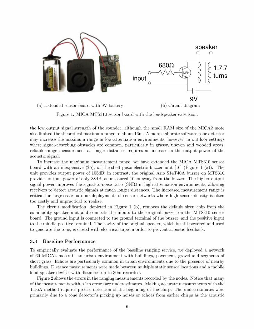
Figure 1: MICA MTS310 sensor board with the loudspeaker extension.

the low output signal strength of the sounder, although the small RAM size of the MICA2 motealso limited the theoretical maximum range to about 16m. A more elaborate software tone detectormay increase the maximum range in low-attenuation environments; however, in outdoor settingswhere signal-absorbing obstacles are common, particularly in grassy, uneven and wooded areas,reliable range measurement at longer distances requires an increase in the output power of theacoustic signal.

To increase the maximum measurement range, we have extended the MICA MTS310 sensorboard with an inexpensive ($5), off-the-shelf piezo-electric buzzer unit [16] (Figure 1 (a)). Theunit provides output power of 105dB; in contrast, the original Ario S14T40A buzzer on MTS310provides output power of only 88dB, as measured 10cm away from the buzzer. The higher outputsignal power improves the signal-to-noise ratio (SNR) in high-attenuation environments, allowingreceivers to detect acoustic signals at much longer distances. The increased measurement range iscritical for large-scale outdoor deployments of sensor networks where high sensor density is oftentoo costly and impractical to realize.

The circuit modification, depicted in Figure 1 (b), removes the default siren chip from thecommodity speaker unit and connects the inputs to the original buzzer on the MTS310 sensorboard. The ground input is connected to the ground terminal of the buzzer, and the positive inputto the middle positive terminal. The cavity of the original speaker, which is still powered and usedto generate the tone, is closed with electrical tape in order to prevent acoustic feedback.

3.3 Baseline Performance

To empirically evaluate the performance of the baseline ranging service, we deployed a networkof 60 MICA2 motes in an urban environment with buildings, pavement, gravel and segments ofshort grass. Echoes are particularly common in urban environments due to the presence of nearbybuildings. Distance measurements were made between multiple static sensor locations and a mobileloud speaker device, with distances up to 30m recorded.

Figure 2 shows the errors in the ranging measurements recorded by the nodes. Notice that manyof the measurements with >1m errors are underestimates. Making accurate measurements with theTDoA method requires precise detection of the beginning of the chirp. The underestimates wereprimarily due to a tone detector’s picking up noises or echoes from earlier chirps as the acoustic

6

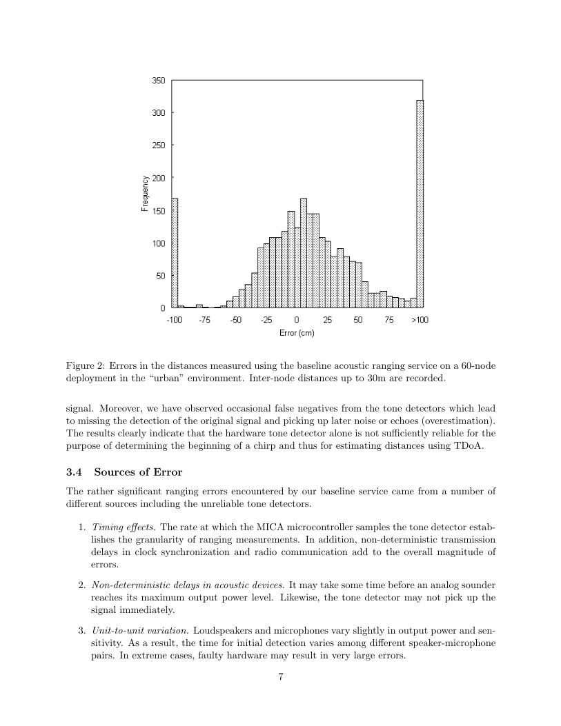
Figure 2: Errors in the distances measured using the baseline acoustic ranging service on a 60-nodedeployment in the “urban” environment. Inter-node distances up to 30m are recorded.

signal. Moreover, we have observed occasional false negatives from the tone detectors which leadto missing the detection of the original signal and picking up later noise or echoes (overestimation).The results clearly indicate that the hardware tone detector alone is not sufficiently reliable for thepurpose of determining the beginning of a chirp and thus for estimating distances using TDoA.

3.4 Sources of Error

The rather significant ranging errors encountered by our baseline service came from a number ofdifferent sources including the unreliable tone detectors.

1. Timing effects. The rate at which the MICA microcontroller samples the tone detector estab-lishes the granularity of ranging measurements. In addition, non-deterministic transmissiondelays in clock synchronization and radio communication add to the overall magnitude oferrors.

2. Non-deterministic delays in acoustic devices. It may take some time before an analog sounderreaches its maximum output power level. Likewise, the tone detector may not pick up thesignal immediately.

3. Unit-to-unit variation. Loudspeakers and microphones vary slightly in output power and sen-sitivity. As a result, the time for initial detection varies among different speaker-microphonepairs. In extreme cases, faulty hardware may result in very large errors.

7

4. Signal attenuation. Sensor nodes experience different signal attenuation depending on envi-ronmental factors, such as height of grass and presence or absence of trees or bushes, whichaffect the reliability of signal detection.

5. Noise. Noise in frequency bands close to that of the beacon signal frequency as well aswide-band noise may cause false positives.

6. Echoes. Due to multi-path effects, some sensors can only hear echoes of the original signal,and not the signal itself. Also, echoes may interfere with the original signal to cancel out thesignal or amplify other noises.

7. Unreliable tone detection. The tone detector in the MICA sensor board does not alwayscorrectly indicate the presence or absence of a signal and thus may trigger false detections.

These sources of error have some distinctive characteristics. We expect errors from sources 1,2 and 3 follow a mostly Gaussian distribution with a fairly small variance. Errors due to source4 are likely to be geographically correlated, whereas those from sources 5 and 6 may or may notbe correlated, depending on the environment. In the following section, we describe techniques wehave incorporated into our refined ranging service to reduce the effects of these errors.

3.5 Refined Approach

Taking into consideration the sources of error listed above, we have improved on the baseline rangingservice by adopting a more sophisticated detection mechanism and performing statistical filteringand consistency checking on the results.

Signal Detection

As discussed in Section 3.3, the tone detector device of the MICA sensor board is not very reliable.It sometimes fails to recognize the presence of a signal, particularly at high sampling rates, andother times it returns false positives when no sound other than background noise is present. Wehave also observed throughout the experiments that the probability of false detection is stronglyaffected by environmental conditions at the time of measurement (e.g., background noise andsignal attenuation). Fortunately, the probability of detecting a tone, P [b(t) = 1], is much higherwhen a tone is actually present than when only background noise is present. This separationhas enabled us to model the output of this tone detector as a binary time series b(t), whereP [b(t) = 1|signal present] P [b(t) = 1|no signal present].

Based on this model, we improve the confidence of acoustic signal detection by combiningmultiple sampling results of the tone detector before searching for the beginning of the signal.For our purposes, simple addition suffices, i.e., we add the binary outputs of the tone detectorfrom several ranging attempts in a manner which amplifies tone detections occurring in the samepositions in multiple attempts. Since the starting time of a signal at a receiver depends on itsdistance from the source, we know the starting positions of multiple signals sent between the twonodes are correlated. On the other hand, when random background noise (e.g., birds’ chirping,wind noise, footsteps) triggers the detector, the probability that it will be repeated in the sameposition is very small. Once a sufficient number of sampling results are accumulated, we applythreshold detection to make the final judgment: the sum of the binary samples must exceed thethreshold value for positive detection to be recorded for that sample, and this must happen for asufficient number of nearby samples for a chirp to be recognized.

8

To make signal detection more resistant to echoes and background noise, we encode a patternin the acoustic signal emitted from the source node. Currently, we use a very simple pattern—asequence of identical chirps interspersed with intervals of silence. When detecting the signal, we lookat both the chirp and the interval preceding it, allowing us to identify false detections due to noiseor echoes that are not part of the pattern. To counteract the effect of echoes of the original chirpbeing detected, we include small random delays, between elements of the pattern. For identifyingthe tone itself, we apply threshold detection at the receiver and require k positive detections outof n consecutive samples to identify the signal pattern. We plan to experiment with more complexpatterns to examine their effectiveness in reducing the number of incorrect measurements due toechoes and noise. In summary, we compute the detection time series detect(t) as

detect(t) = truefn

n∑

i=0

truefn

m∑

j=0

bj(t− i) > T

> k

where m is the number of samples accumulated, T is the threshold for signal detection, n is thetotal number of signal detections, k is the threshold for pattern identification, and truefn(x) = 1 ifx is true and 0 otherwise. The beginning of the acoustic signal is determined as the minimum valueof t that satisfies detect(t) = 1. Figure 3 shows the pseudocode of the signal detection algorithm.

Statistical Filtering

Even with the improved signal detection algorithm, individual range estimates may still be erro-neous, albeit less frequently, due to a threshold setting that is too low, hardware malfunction, orsome other causes, such as another nearby node chirping out of turn. Assuming that the errors arenot correlated, we make multiple distance measurements for a pair of nodes and apply statisticalfiltering to yield a more stable and accurate estimate of the actual distance. Depending on thenumber of measurements, we take the median or mode value of the measurements, which limitsthe effect of outliers. The mode operation is more resistant to the effects of uncorrelated outliersthan the median, but it needs more measurements to be effective. The statistical filtering is quiteeffective at discounting uncorrelated errors caused by random, one-time events. Figure 4 shows theperformance of the baseline ranging service when employing the median filtering.

Consistency Checking

The ranging service employs consistency checks to identify measurements containing errors thatmay be correlated on a single node (e.g., errors due to faulty hardware or persistent wide-bandnoise). These checks involve comparison of data between multiple nodes. For example, bidirectionalrange estimates between a pair of nodes are discarded if they are inconsistent. If three nodeshave measurements to each other, we use the triangle inequality 2 to identify inconsistent one. Acaveat is none of these can identify which of the measurements is incorrect with complete certainty.Sometimes it may be beneficial to retain suspicious measurements due to the scarcity of availabledata.

3.5.1 Deployment Constraints

Some sensor network deployments offer additional information about sensor placement. For exam-ple, a deployment may have a requirement of minimum node separation. Rough distance estimates

2The estimates of two sides of the triangle add up to less than the third.

9

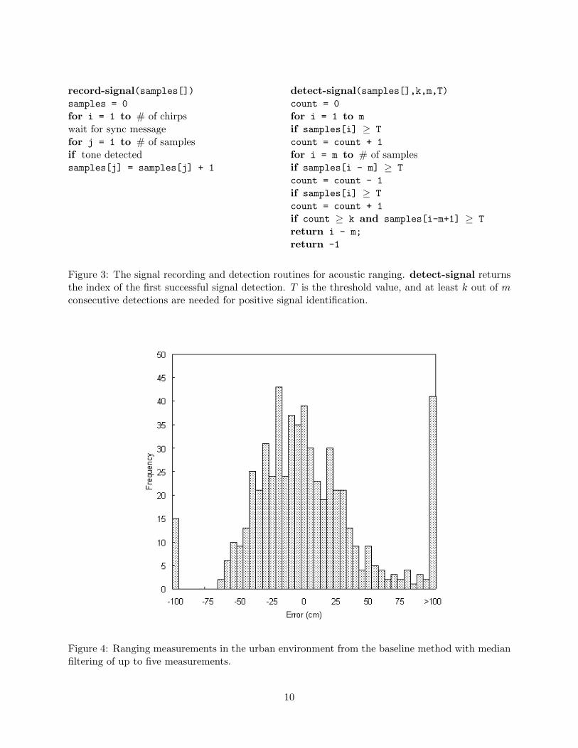
record-signal(samples[])samples = 0for i = 1 to # of chirpswait for sync messagefor j = 1 to # of samplesif tone detectedsamples[j] = samples[j] + 1

detect-signal(samples[],k,m,T)count = 0for i = 1 to mif samples[i] ≥ Tcount = count + 1for i = m to # of samplesif samples[i - m] ≥ Tcount = count - 1if samples[i] ≥ Tcount = count + 1if count ≥ k and samples[i-m+1] ≥ Treturn i - m;return -1

Figure 3: The signal recording and detection routines for acoustic ranging. detect-signal returnsthe index of the first successful signal detection. T is the threshold value, and at least k out of mconsecutive detections are needed for positive signal identification.

Figure 4: Ranging measurements in the urban environment from the baseline method with medianfiltering of up to five measurements.

10

can be made based on node density and network hop count before the ranging service starts. Ona regular grid deployment, a set of possible inter-node distances can be deduced from the size andshape of the grid configuration. These data provide additional constraints that consistent rang-ing measurements should satisfy. We plan to incorporate more advanced filtering and consistencychecking based on these constraints in the ranging service.

3.6 Experimental Evaluation

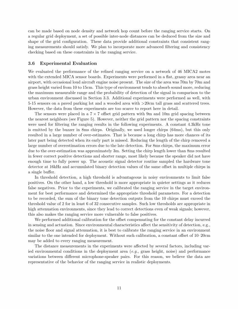
We evaluated the performance of the refined ranging service on a network of 46 MICA2 moteswith the extended MICA sensor boards. Experiments were performed in a flat, grassy area near anairport, with occasional loud aircraft engine noise present. The size of the area was 70m by 70m andgrass height varied from 10 to 15cm. This type of environment tends to absorb sound more, reducingthe maximum measurable range and the probability of detection of the signal in comparison to theurban environment discussed in Section 3.3. Additional experiments were performed as well, with5-15 sensors on a paved parking lot and a wooded area with >20cm tall grass and scattered trees.However, the data from these experiments are too scarce to report here in detail.

The sensors were placed in a 7 × 7 offset grid pattern with 9m and 10m grid spacing betweenthe nearest neighbors (see Figure 5). However, neither the grid pattern nor the spacing constraintswere used for filtering the ranging results in the following experiments. A constant 4.3kHz toneis emitted by the buzzer in 8ms chirps. Originally, we used longer chirps (64ms), but this onlyresulted in a large number of over-estimates. That is because a long chirp has more chances of itslater part being detected when its early part is missed. Reducing the length of the chirp removed alarge number of overestimation errors due to the late detection. For 8ms chirps, the maximum errordue to the over-estimation was approximately 3m. Setting the chirp length lower than 8ms resultedin fewer correct positive detections and shorter range, most likely because the speaker did not haveenough time to fully power up. The acoustic signal detector routine sampled the hardware tonedetector at 16kHz and accumulated binary detection values of the same offset in multiple chirps ina single buffer.

In threshold detection, a high threshold is advantageous in noisy environments to limit falsepositives. On the other hand, a low threshold is more appropriate in quieter settings as it reducesfalse negatives. Prior to the experiments, we calibrated the ranging service in the target environ-ment for best performance and determined the appropriate threshold parameters. For a detectionto be recorded, the sum of the binary tone detection outputs from the 10 chirps must exceed thethreshold value of 2 for in least 6 of 32 consecutive samples. Such low thresholds are appropriate inhigh attenuation environments, since they lead to correct detections even of weak signals; however,this also makes the ranging service more vulnerable to false positives.

We performed additional calibration for the offset compensating for the constant delay incurredin sensing and actuation. Since environmental characteristics affect the sensitivity of detection, e.g.,the noise floor and signal attenuation, it is best to calibrate the ranging service in an environmentsimilar to the one intended for deployment. Without such calibration, a constant offset of 10–20cmmay be added to every ranging measurement.

The distance measurements in the experiments were affected by several factors, including var-ied environmental conditions in the deployment area (e.g., grass height, noise) and performancevariations between different microphone-speaker pairs. For this reason, we believe the data arerepresentative of the behavior of the ranging service in realistic deployments.

11

0

10

20

30

40

50

60

0 10 20 30 40 50 60

Dis

tanc

e (m

)

Distance (m)

actual position

Figure 5: An offset grid deployment pattern with 9m and 10m node spacing.

3.6.1 Analysis: Accuracy

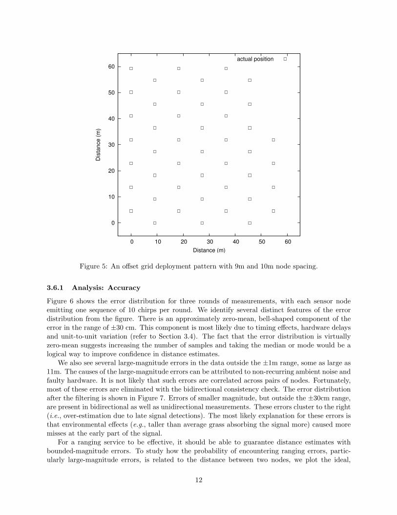
Figure 6 shows the error distribution for three rounds of measurements, with each sensor nodeemitting one sequence of 10 chirps per round. We identify several distinct features of the errordistribution from the figure. There is an approximately zero-mean, bell-shaped component of theerror in the range of ±30 cm. This component is most likely due to timing effects, hardware delaysand unit-to-unit variation (refer to Section 3.4). The fact that the error distribution is virtuallyzero-mean suggests increasing the number of samples and taking the median or mode would be alogical way to improve confidence in distance estimates.

We also see several large-magnitude errors in the data outside the ±1m range, some as large as11m. The causes of the large-magnitude errors can be attributed to non-recurring ambient noise andfaulty hardware. It is not likely that such errors are correlated across pairs of nodes. Fortunately,most of these errors are eliminated with the bidirectional consistency check. The error distributionafter the filtering is shown in Figure 7. Errors of smaller magnitude, but outside the ±30cm range,are present in bidirectional as well as unidirectional measurements. These errors cluster to the right(i.e., over-estimation due to late signal detections). The most likely explanation for these errors isthat environmental effects (e.g., taller than average grass absorbing the signal more) caused moremisses at the early part of the signal.

For a ranging service to be effective, it should be able to guarantee distance estimates withbounded-magnitude errors. To study how the probability of encountering ranging errors, partic-ularly large-magnitude errors, is related to the distance between two nodes, we plot the ideal,

12

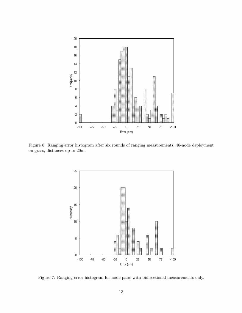
Figure 6: Ranging error histogram after six rounds of ranging measurements, 46-node deploymenton grass, distances up to 20m.

Figure 7: Ranging error histogram for node pairs with bidirectional measurements only.

13

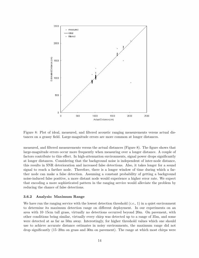
Figure 8: Plot of ideal, measured, and filtered acoustic ranging measurements versus actual dis-tances on a grassy field. Large-magnitude errors are more common at longer distances.

measured, and filtered measurements versus the actual distances (Figure 8). The figure shows thatlarge-magnitude errors occur more frequently when measuring over a longer distance. A couple offactors contribute to this effect. In high-attenuation environments, signal power drops significantlyat longer distances. Considering that the background noise is independent of inter-node distance,this results in SNR deterioration and increased false detections. Also, it takes longer for a soundsignal to reach a farther node. Therefore, there is a longer window of time during which a far-ther node can make a false detection. Assuming a constant probability of getting a backgroundnoise-induced false positive, a more distant node would experience a higher error rate. We expectthat encoding a more sophisticated pattern in the ranging service would alleviate the problem byreducing the chance of false detections.

3.6.2 Analysis: Maximum Range

We have run the ranging service with the lowest detection threshold (i.e., 1) in a quiet environmentto determine its maximum detection range on different deployment. In our experiments on anarea with 10–15cm tall grass, virtually no detections occurred beyond 20m. On pavement, withother conditions being similar, virtually every chirp was detected up to a range of 35m, and somewere detected at as far as 50m away. Interestingly, for higher threshold values which one shoulduse to achieve accurate distance estimates in noisy environments, the maximum range did notdrop significantly (15–20m on grass and 30m on pavement). The range at which most chirps were

14

consistently detected (about 80–85%) was 10 and 25m on grass and pavement, respectively. Thiseffect is most likely due to the increase in SNR induced by accumulating multiple measurements.

It should be noted, however, that we have observed that some speaker-microphone pairs haveranges that are consistently much shorter or much longer than the typical values presented above.We suspect this happens due to unit-to-unit variations in loudspeaker power output and microphonesensitivity. The microphones are rated at ±3dB sensitivity, and we have observed variations of upto 5dB on the loudspeakers.

The theoretical maximum range of the service is closed related to the buffer space availablein the underlying WSN platform. The buffer space required for our service is determined by thedesired maximum measurable distance and the number of samples accumulated per measurement.We allocate 4 bits for each offset of the buffer, which allows samples from up to 15 chirps to beaccumulated. For 15 samples at distances up to 20m, the service uses less than 500 bytes of RAM.It uses the tone detector of the MICA sensor board to reduce the memory footprint at the expenseof reliability and accuracy. We offset the loss of accuracy using signal processing and statisticalfiltering techniques. This is a significant improvement over the ranging service described in [17]which fills all available buffer space in the MICA2 mote platform only to achieve a maximum rangeof less than 16m. Not only do we extend the maximum measurable range, but also leave enoughRAM available for other applications to run concurrently with the ranging service. To the best ofour knowledge, this is the first fully-functional ranging service for wireless sensor networks whichfeatures long range, high precision, and a relatively small memory footprint.

3.7 Alternative Tone Detection

The acoustic ranging solution described above assumes availability of a fixed-frequency buzzerand a matching hardware tone detector in the WSN platform. However, not all wireless sensorplatforms come equipped with the devices. Instead, some provide more general acoustic sensingand actuation features, such as a pulse width modulation (PWM) buzzer and tunable band-passfilter for the microphone (e.g., Crossbow’s XSM mote). Emulating MICA’s acoustic features onthese platforms (i.e., tuning the buzzer and filters to a fixed frequency and performing simpleenergy detection) may not be sufficient due to the low signal-to-noise ratio when making rangingmeasurements over long distances. For example, we have found from preliminary tests on the XSMplatform that a narrow setting of its hardware bandpass filter combined with energy detectionachieves similar accuracy as the MICA hardware tone detector, but a shorter maximum range(10m).

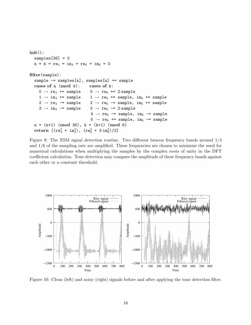
To support the acoustic ranging solution on platforms where a hardware tone detector is notavailable, we have designed a digital signal processing filter3 based on the Discrete Fourier Trans-form (DFT)4 [4]. While the standard DFT algorithm calculates the amplitude of each frequencycomponent of a signal, for tone detection purposes we only need to know the amplitude of thebeacon signal’s frequency component. In order to reduce changes of false positive detection, itis useful to automatically isolate the amplitude of noise and subtract it from the DFT output; apositive result indicates detection of a tone. We evaluate DFT for all frequency components andaverage the results to calculate this amplitude. The pseudo code of the tone detection algorithm isin Figure 9. Figure 10 depicts the tone detection filter’s outputs for a clean and a noisy signal con-taining periodic constant-frequency chirps. In the latter case, three of the four chirps are correctlydetected, with no false positives.

3We hasten to note that detection using the filter has not been fully tested and more experiments are needed toempirically assess the filter’s performance and fine-tune this approach.

4In practice, FFT would be used instead of simple DFT.

15

init():samples[36] = 0n = k = re4 = im4 = re6 = im6 = 0

filter(sample):sample -= samples[n], samples[n] += samplecases of n (mod 4): cases of k:

0 → re4 += sample 0 → re6 += 2·sample1 → im4 += sample 1 → re6 += sample, im6 += sample2 → re4 -= sample 2 → re6 -= sample, im6 += sample3 → im4 -= sample 3 → re6 -= 2·sample

4 → re6 -= sample, im6 -= sample5 → re6 += sample, im6 -= sample

n = (n+1) (mod 36), k = (k+1) (mod 6)return [(re2

4 + im24), (re2

6 + 3·im26)/2]

Figure 9: The XSM signal detection routine. Two different beacon frequency bands around 1/4and 1/6 of the sampling rate are amplified. These frequencies are chosen to minimize the need fornumerical calculations when multiplying the samples by the complex roots of unity in the DFTcoefficient calculation. Tone detection may compare the amplitude of these frequency bands againsteach other or a constant threshold.

−1500

−1000

−500

0

500

1000

0 100 200 300 400 500 600 700 800

Am

plitu

de

Time

Raw signalFiltered signal

−1500

−1000

−500

0

500

1000

0 100 200 300 400 500 600 700 800

Am

plitu

de

Time

Raw signalFiltered signal

Figure 10: Clean (left) and noisy (right) signals before and after applying the tone detection filter.

16

Because the ranging service with the software tone detector needs to store a sum of raw sampledvalues rather than a sum of 1-bit output values from a hardware tone detector, its memory require-ment is considerably larger than that of its hardware counterpart. To achieve a maximum rangeof 20m, a 2kB buffer is required with a sampling rate of 16kHz. Depending on the environmentand the characteristics of the acoustic signal, a slower sampling rate or a smaller number of bitsrecorded per sample may increase the maximum range when given a fixed amount of buffer space.

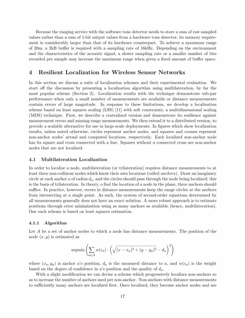
4 Resilient Localization for Wireless Sensor Networks

In this section we discuss a suite of localization schemes and their experimental evaluation. Westart off the discussion by presenting a localization algorithm using multilateration, by far themost popular scheme (Section 2). Localization results with the technique demonstrate sub-parperformance when only a small number of measurements are available or distance measurementscontain errors of large magnitude. In response to these limitations, we develop a localizationscheme based on least squares scaling (LSS) [11] with soft constraints, a multidimensional scaling(MDS) technique. First, we describe a centralized version and demonstrate its resilience againstmeasurement errors and missing range measurements. We then extend it to a distributed version, toprovide a scalable alternative for use in large-scale deployments. In figures which show localizationresults, unless noted otherwise, circles represent anchor nodes, and squares and crosses representnon-anchor nodes’ actual and computed locations, respectively. Each localized non-anchor nodehas its square and cross connected with a line. Squares without a connected cross are non-anchornodes that are not localized.

4.1 Multilateration Localization

In order to localize a node, multilateration (or trilateration) requires distance measurements to atleast three non-collinear nodes which know their own locations (called anchors). Draw an imaginarycircle at each anchor a of radius da, and the circles should pass through the node being localized; thisis the basis of trilateration. In theory, o find the location of a node in the plane, three anchors shouldsuffice. In practice, however, errors in distance measurements keep the range circles at the anchorsfrom intersecting at a single point. As such, the system of second-order equations determined byall measurements generally does not have an exact solution. A more robust approach is to estimatepositions through error minimization using as many anchors as available (hence, multilateration).One such scheme is based on least squares estimation.

4.1.1 Algorithm

Let A be a set of anchor nodes to which a node has distance measurements. The position of thenode (x, y) is estimated as

argmin

(∑a∈A

w(ca) ·(√

(x− xa)2 + (y − ya)2 − da

)2)

where (xa, ya) is anchor a’s position, da is the measured distance to a, and w(ca) is the weightbased on the degree of confidence in a’s position and the quality of da.

With a slight modification we can devise a scheme which progressively localizes non-anchors soas to increase the number of anchors used per non-anchor. Non-anchors with distance measurementsto sufficiently many anchors are localized first. Once localized, they become anchor nodes and are

17

used to localize the remaining non-anchors. In this progressive localization, different anchors maybe assigned different weights depending on the quality of range measurements (da) as well as onassociated localization errors (E) if they were originally non-anchors and subsequently localized.For the experiments reported below, we did not use this proposed modification; rather, we usedthe original set of anchors only and assigned a constant weight of 1 to all anchors.

4.1.2 Intersection Consistency Checking

Like other least squares estimation techniques, multilateration via least squares is sensitive tonoisy measurements. We improve resistance to measurement errors by cross-checking consistencyof distance measurements and throwing out inconsistent data.

The consistency check is based on the following simple observation. Recall that errors in distancemeasurements to anchors would not allow the corresponding range circles to intersect at a singlepoint. Rather, some intersection points of the circles would form a cluster around the node beinglocalized. For an anchor with a sufficiently accurate distance measurement, its range circle shouldhave intersection points close to other consistent anchors’ intersection points.

Exploiting this observation, we compute intersection points of all pairs of circles and drop fromconsideration those anchors which have no intersection points close to other intersection points (e.g.,beyond 1m range). The remaining anchor nodes, i.e., those with consistent distance estimates, areused for localization. Note that we may take the mode of the intersection points of the remaininganchors instead of minimizing the error if the number of anchors is large enough.

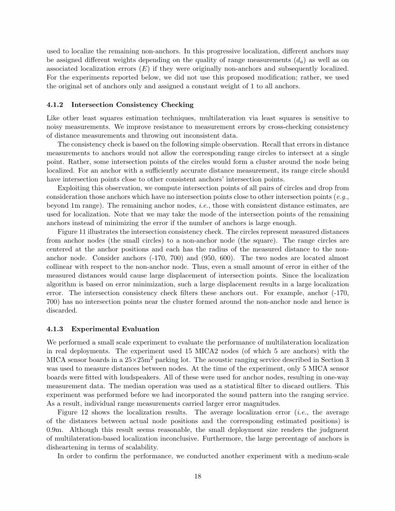
Figure 11 illustrates the intersection consistency check. The circles represent measured distancesfrom anchor nodes (the small circles) to a non-anchor node (the square). The range circles arecentered at the anchor positions and each has the radius of the measured distance to the non-anchor node. Consider anchors (-170, 700) and (950, 600). The two nodes are located almostcollinear with respect to the non-anchor node. Thus, even a small amount of error in either of themeasured distances would cause large displacement of intersection points. Since the localizationalgorithm is based on error minimization, such a large displacement results in a large localizationerror. The intersection consistency check filters these anchors out. For example, anchor (-170,700) has no intersection points near the cluster formed around the non-anchor node and hence isdiscarded.

4.1.3 Experimental Evaluation

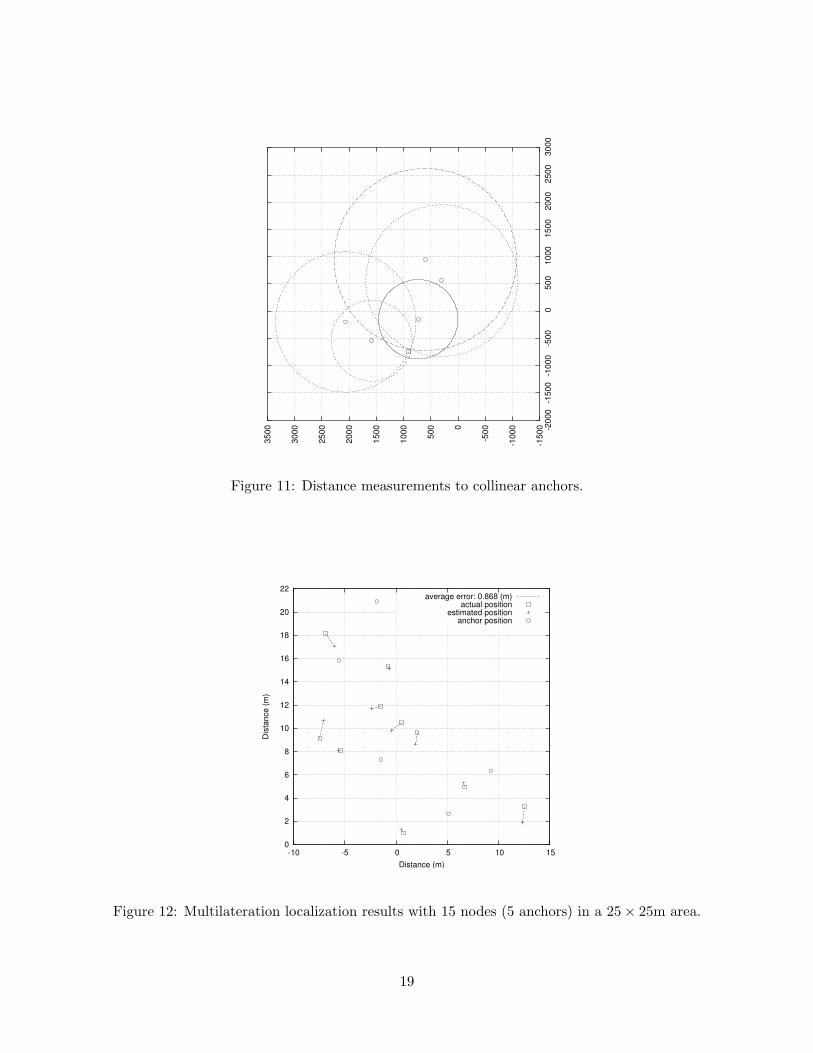
We performed a small scale experiment to evaluate the performance of multilateration localizationin real deployments. The experiment used 15 MICA2 nodes (of which 5 are anchors) with theMICA sensor boards in a 25×25m2 parking lot. The acoustic ranging service described in Section 3was used to measure distances between nodes. At the time of the experiment, only 5 MICA sensorboards were fitted with loudspeakers. All of these were used for anchor nodes, resulting in one-waymeasurement data. The median operation was used as a statistical filter to discard outliers. Thisexperiment was performed before we had incorporated the sound pattern into the ranging service.As a result, individual range measurements carried larger error magnitudes.

Figure 12 shows the localization results. The average localization error (i.e., the averageof the distances between actual node positions and the corresponding estimated positions) is0.9m. Although this result seems reasonable, the small deployment size renders the judgmentof multilateration-based localization inconclusive. Furthermore, the large percentage of anchors isdisheartening in terms of scalability.

In order to confirm the performance, we conducted another experiment with a medium-scale

18

-150

0

-100

0

-500 0

500

100

0

150

0

200

0

250

0

300

0

350

0 -200

0-1

500

-100

0-5

00 0

500

100

0 1

500

200

0 2

500

300

0

Figure 11: Distance measurements to collinear anchors.

0

2

4

6

8

10

12

14

16

18

20

22

-10 -5 0 5 10 15

Dis

tanc

e (m

)

Distance (m)

average error: 0.868 (m)actual position

estimated positionanchor position

Figure 12: Multilateration localization results with 15 nodes (5 anchors) in a 25× 25m area.

19

0

10

20

30

40

50

60

70

0 10 20 30 40 50 60

Dis

tanc

e (m

)

Distance (m)

anchorsactual position

dm-dr < -1 (m)-1 < dm-dr < 1 (m)

dm-dr > 1 (m)

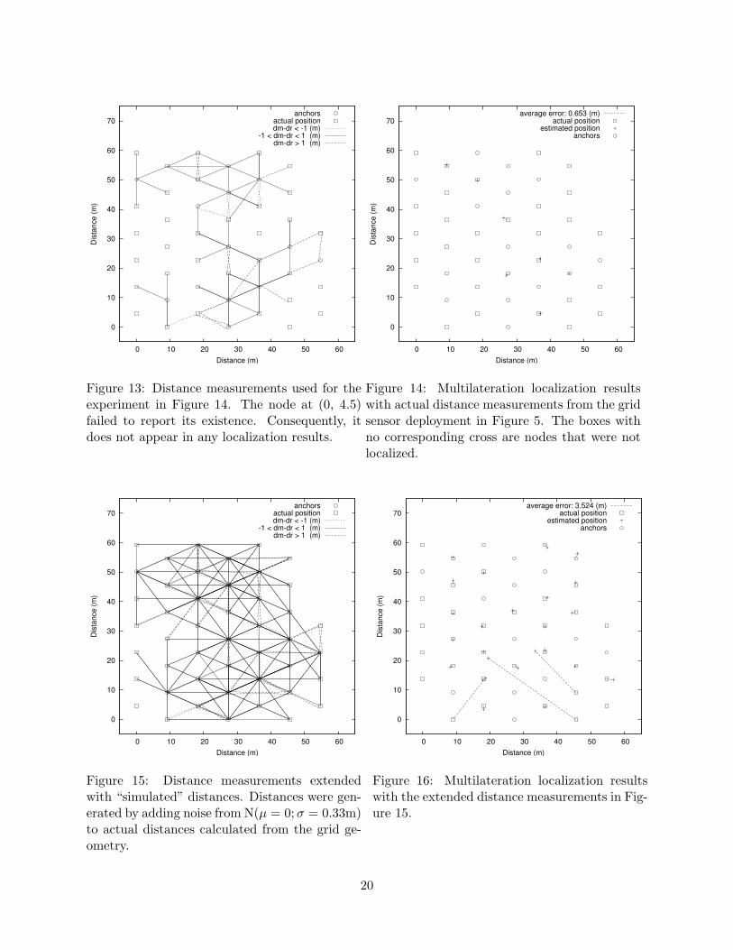
Figure 13: Distance measurements used for theexperiment in Figure 14. The node at (0, 4.5)failed to report its existence. Consequently, itdoes not appear in any localization results.

0

10

20

30

40

50

60

70

0 10 20 30 40 50 60

Dis

tanc

e (m

)

Distance (m)

average error: 0.653 (m)actual position

estimated positionanchors

Figure 14: Multilateration localization resultswith actual distance measurements from the gridsensor deployment in Figure 5. The boxes withno corresponding cross are nodes that were notlocalized.

0

10

20

30

40

50

60

70

0 10 20 30 40 50 60

Dis

tanc

e (m

)

Distance (m)

anchorsactual position

dm-dr < -1 (m)-1 < dm-dr < 1 (m)

dm-dr > 1 (m)

Figure 15: Distance measurements extendedwith “simulated” distances. Distances were gen-erated by adding noise from N(µ = 0;σ = 0.33m)to actual distances calculated from the grid ge-ometry.

0

10

20

30

40

50

60

70

0 10 20 30 40 50 60

Dis

tanc

e (m

)

Distance (m)

average error: 3.524 (m)actual position

estimated positionanchors

Figure 16: Multilateration localization resultswith the extended distance measurements in Fig-ure 15.

20

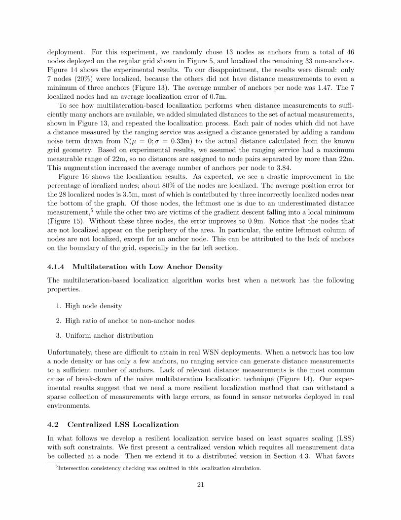
deployment. For this experiment, we randomly chose 13 nodes as anchors from a total of 46nodes deployed on the regular grid shown in Figure 5, and localized the remaining 33 non-anchors.Figure 14 shows the experimental results. To our disappointment, the results were dismal: only7 nodes (20%) were localized, because the others did not have distance measurements to even aminimum of three anchors (Figure 13). The average number of anchors per node was 1.47. The 7localized nodes had an average localization error of 0.7m.

To see how multilateration-based localization performs when distance measurements to suffi-ciently many anchors are available, we added simulated distances to the set of actual measurements,shown in Figure 13, and repeated the localization process. Each pair of nodes which did not havea distance measured by the ranging service was assigned a distance generated by adding a randomnoise term drawn from N(µ = 0; σ = 0.33m) to the actual distance calculated from the knowngrid geometry. Based on experimental results, we assumed the ranging service had a maximummeasurable range of 22m, so no distances are assigned to node pairs separated by more than 22m.This augmentation increased the average number of anchors per node to 3.84.

Figure 16 shows the localization results. As expected, we see a drastic improvement in thepercentage of localized nodes; about 80% of the nodes are localized. The average position error forthe 28 localized nodes is 3.5m, most of which is contributed by three incorrectly localized nodes nearthe bottom of the graph. Of those nodes, the leftmost one is due to an underestimated distancemeasurement,5 while the other two are victims of the gradient descent falling into a local minimum(Figure 15). Without these three nodes, the error improves to 0.9m. Notice that the nodes thatare not localized appear on the periphery of the area. In particular, the entire leftmost column ofnodes are not localized, except for an anchor node. This can be attributed to the lack of anchorson the boundary of the grid, especially in the far left section.

4.1.4 Multilateration with Low Anchor Density

The multilateration-based localization algorithm works best when a network has the followingproperties.

1. High node density

2. High ratio of anchor to non-anchor nodes

3. Uniform anchor distribution

Unfortunately, these are difficult to attain in real WSN deployments. When a network has too lowa node density or has only a few anchors, no ranging service can generate distance measurementsto a sufficient number of anchors. Lack of relevant distance measurements is the most commoncause of break-down of the naive multilateration localization technique (Figure 14). Our exper-imental results suggest that we need a more resilient localization method that can withstand asparse collection of measurements with large errors, as found in sensor networks deployed in realenvironments.

4.2 Centralized LSS Localization

In what follows we develop a resilient localization service based on least squares scaling (LSS)with soft constraints. We first present a centralized version which requires all measurement databe collected at a node. Then we extend it to a distributed version in Section 4.3. What favors

5Intersection consistency checking was omitted in this localization simulation.

21

LSS over classical MDS for localization of sensor nodes is that LSS-based localization does notrequire distance measurements between all pairs of nodes. Even with some missing distance mea-surements, it still yields acceptable localization results. Moreover, we may use different weights fordistance measurements depending on their confidence levels and easily incorporate constraints suchas minimum node separation into the minimization process to further improve localization results.

4.2.1 Algorithm

Multidimensional scaling is “any procedure which starts with the ‘distance’ between a set of pointsand finds a configuration of points, preferably, in a small number of dimensions, usually 2 or3” [11]. Here, a configuration refers to a set of coordinate values. When distances between nodesare available, MDS [19, 18, 11] finds their relative coordinates. In localization using classicalMDS, the input distance matrix is transformed to a quadratic matrix of coordinates via doubleaveraging. Then, singular value decomposition (SVD) is applied to the quadratic matrix to getits principal components. The first two principal components are the configuration sought. Onecritical requirement is that distances between all pairs of nodes be known a priori.

An alternative technique is LSS [11], which seeks a configuration C = (xi, yi) : i = 1, . . . , nfrom a set of distances Dfull = dij : i, j = 1, . . . , n by minimizing the unweighted error functionEu:

Eu =∑

dij∈Dfull

(√(xi − xj)2 + (yi − yj)2 − dij

)2

where dij is the distance between points (xi, yi) and (xj , yj). An important property of LSS is thatit still works using only a subset of Dfull. This property allows LSS-based localization to toleratesparse measurement data.

The error function is the sum of squares of differences between estimated distances and cor-responding measured distances. As a result, errors in distance measurement are squared, too.Therefore, weighting distance measurements according to their confidence helps limit the effect ofmeasurement errors on localization results. Statistical entities (e.g., standard deviation) can makea good choice for such weights. We extend the error function Eu to accommodate different weightsby defining Ew:

Ew =∑

dij∈D

wij ·(√

(xi − xj)2 + (yi − yj)2 − dij

)2

where D ⊆ Dfull is a set of distance measurements from a ranging service.In many sensor deployments, a minimum distance between nodes can be known in advance.

LSS allows us to incorporate this minimum spacing constraint into localization as a soft constraint[7]. Using the soft constraint we penalize pairs of nodes which do not have distance measurementsfrom the ranging service and whose assigned coordinates violate the minimum spacing constraintso that any output solution would become more consistent. This can be visualized as straighteninga plane which is incorrectly folded. Note that the set of penalized pairs dynamically changes asminimization progresses. With the soft constraint, the error function which we seek to minimizebecomes:

E = Ew +∑

dij 6∈D

wD ·(

min

(√(xi − xj)2 + (yi − yj)2, dmin

)− dmin

)2

22

where dmin is the minimum node spacing and wD is the weight for the soft constraint. Note thatwij = 0 for pairs of nodes which do not have distance measurements in D.

We use gradient descent to find a configuration that minimizes the error term. We updatecoordinates of the nodes at each time step using the rules

[xt+1,yt+1] = [xt,yt]− α · ∇E|[xt,yt] (1)

where α is a step size and ∇E = [ ∂E∂x1

, . . . , ∂E∂xn

, ∂E∂y1

, . . . , ∂E∂yn

] is the gradient of E. Without the softconstraint,

∂E

∂xi

∣∣∣∣[xt,yt]

=∂Eunconstrained

∂xi

∣∣∣∣[xt,yt]

= wij ·∑

dij∈D

(dcompij − dij) · (xt

i − xtj)/dcomp

ij

where dcompij =

√(xt

i − xtj)2 + (yt

i − ytj)2. With the soft constraint, if dij is not defined and dcomp

ij <

dmin,

∂E

∂xi

∣∣∣∣[xt,yt]

=∂Eunconstrained

∂xi

∣∣∣∣[xt,yt]

+ wD ·∑

dij 6∈D

(dcompij − dmin) · (xt

i − xtj)/dcomp

ij .

∂E∂yi

∣∣∣[xt,yt]

can be derived similarly.

To avoid local minima, the gradient descent starts each round of minimization with seed po-sitions obtained by perturbing the best results so far. This process is repeated until a reasonableminimum is reached or the maximum computation time limit expires.

4.2.2 Experimental Evaluation

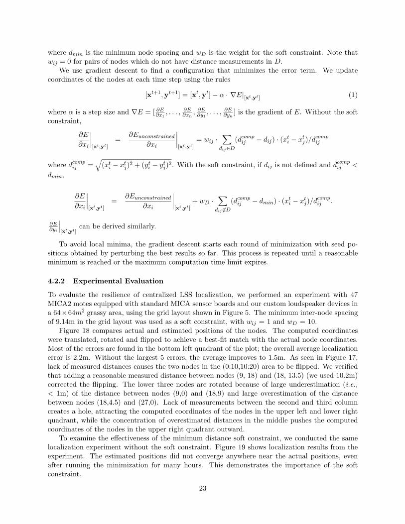
To evaluate the resilience of centralized LSS localization, we performed an experiment with 47MICA2 motes equipped with standard MICA sensor boards and our custom loudspeaker devices ina 64×64m2 grassy area, using the grid layout shown in Figure 5. The minimum inter-node spacingof 9.14m in the grid layout was used as a soft constraint, with wij = 1 and wD = 10.

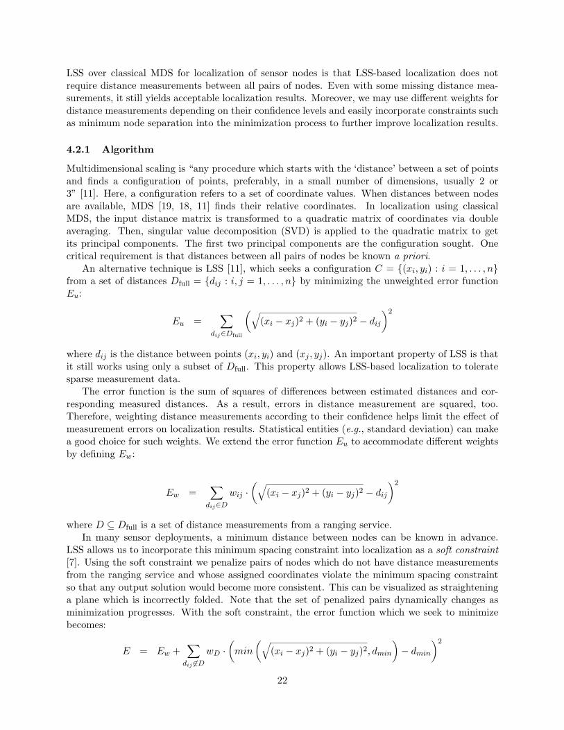
Figure 18 compares actual and estimated positions of the nodes. The computed coordinateswere translated, rotated and flipped to achieve a best-fit match with the actual node coordinates.Most of the errors are found in the bottom left quadrant of the plot; the overall average localizationerror is 2.2m. Without the largest 5 errors, the average improves to 1.5m. As seen in Figure 17,lack of measured distances causes the two nodes in the (0:10,10:20) area to be flipped. We verifiedthat adding a reasonable measured distance between nodes (9, 18) and (18, 13.5) (we used 10.2m)corrected the flipping. The lower three nodes are rotated because of large underestimation (i.e.,< 1m) of the distance between nodes (9,0) and (18,9) and large overestimation of the distancebetween nodes (18,4.5) and (27,0). Lack of measurements between the second and third columncreates a hole, attracting the computed coordinates of the nodes in the upper left and lower rightquadrant, while the concentration of overestimated distances in the middle pushes the computedcoordinates of the nodes in the upper right quadrant outward.

To examine the effectiveness of the minimum distance soft constraint, we conducted the samelocalization experiment without the soft constraint. Figure 19 shows localization results from theexperiment. The estimated positions did not converge anywhere near the actual positions, evenafter running the minimization for many hours. This demonstrates the importance of the softconstraint.

23

0

10

20

30

40

50

60

70

0 10 20 30 40 50 60

Dis

tanc

e (m

)

Distance (m)

actual position dm-dr < -1 (m)

-1 < dm-dr < 1 (m) dm-dr > 1 (m)

Figure 17: Distance measurements used in the LSS localization experiments are the same as theones plotted in Figure 13, except that the latter shows the distances to the anchors only.

0

10

20

30

40

50

60

70

0 10 20 30 40 50 60

Dis

tanc

e (m

)

Distance (m)

average error: 2.229 (m)actual position

estimated position

Figure 18: Centralized LSS localization resultswith the minimum spacing constraint. The av-erage localization error is 2.2m.

0

10

20

30

40

50

60

70

0 10 20 30 40 50 60

Dis

tanc

e (m

)

Distance (m)

average error: 16.609 (m)actual position

estimated position

Figure 19: Centralized LSS localization resultswithout minimum inter-node distance constraintafter a full day of minimization. The computedcoordinates failed to converge to the correspond-ing actual coordinates.

24

-20

-10

0

10

20

30

40

50

60

70

-20 0 20 40 60 80 100

Dis

tanc

e (m

)

Distance (m)

average error: 0.950 (m)actual position

estimated positionanchors

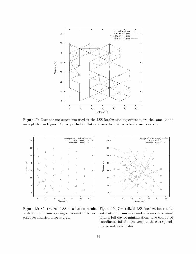
Figure 20: Multilateration localization simula-tion results with a random sensor deployment.

-20

-10

0

10

20

30

40

50

60

70

-20 0 20 40 60 80 100

Dis

tanc

e (m

)

Distance (m)

average error: 0.548 (m)actual position

estimated position

Figure 21: Centralized LSS localization simu-lation results with the minimum distance con-straint.

-20

-10

0

10

20

30

40

50

60

70

-10 0 10 20 30 40 50 60 70 80 90 100

Dis

tanc

e (m

)

Distance (m)

average error: 13.606 (m)actual position

estimated position

Figure 22: Centralized LSS localization simula-tion results without the minimum distance con-straint.

0

1000

2000

3000

4000

5000

6000

7000

8000

9000

0 5 10 15 20 25 30 35 40 45 50

erro

r (E

)

epoch

error (E) without constrainterror (E) with constraint

Figure 23: Changes of errors over time in theminimizations of Figure 21 (with constraint)and Figure 22 (without constraint).

25

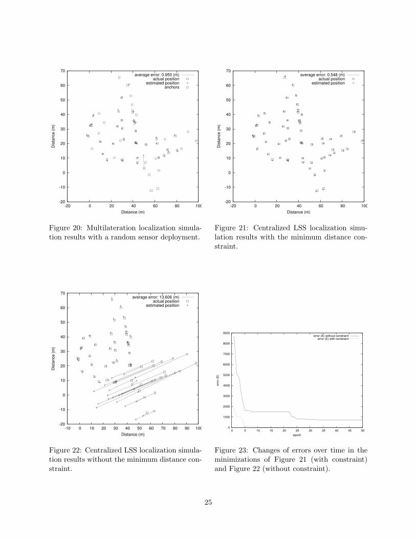
We further performed simulations to compare multilateration to LSS localization using a randomnode deployment. We selected 59 plausible node positions in a map of a few city blocks in a smalltown and randomly designated 18 of them as anchors. Then, we selected 945 pairs of nodes whoseEuclidean distances were less than 22m and perturbed the distances with errors from a Gaussiandistribution N(µ = 0; σ = 0.33m). For LSS localization, we ignored the 18 anchors and insteadregarded them as non-anchors.

The results were as follows: 35 nodes were localized with average localization error of 1.0m.Figures 21 and 22 show the results of the LSS localization with and without the minimum distancesoft constraint, respectively. For the former, we penalized pairs of nodes with unknown distancewhen they were assigned coordinates which made them closer than 9m. All the nodes were localizedwith average error of 0.5m. The results are much better than multilateration, considering thatsome nodes were not localized at all with mulitlateration, while no anchors were used with LSSlocalization. Without the soft constraint, most of the nodes in the lower half were not properlylocalized (Figure 22).

Figure 23 shows how use of the soft constraint helps with error minimization. The error functionhas more terms with the soft constraint than without, which are all positive (because they aresquared terms). Thus, we know that the the error function without constraint terms should have asmaller global minimum. As is evident from the figure, the soft constraint greatly reduces the timeto reach a global minimum.

4.3 Distributed Localization

The centralized LSS localization algorithm is resilient against sparse distance measurements andlarge measurement errors. Unfortunately, it does not scale well as network deployments grow insize. As more nodes are added, the number of terms in the error function increases, as does thenumber of local minima the computation may fall into. In this section, we extend the centralizedLSS localization algorithm to a more scalable distributed version.

4.3.1 Algorithm

The distributed version consists of three steps: local localization, calculating a transform betweenthe local coordinate systems for each pair of neighboring nodes, and alignment of local coordinatesystems to a global coordinate system.

Step 1. Local Localization Each node collects distance measurements to its neighbors as wellas amongst them. A node’s neighbors are nodes to which it has direct distance measurementsfrom the ranging service. Given the measurements, each node uses the LSS localization to find aconfiguration of itself and its neighbors in a local relative coordinate system.

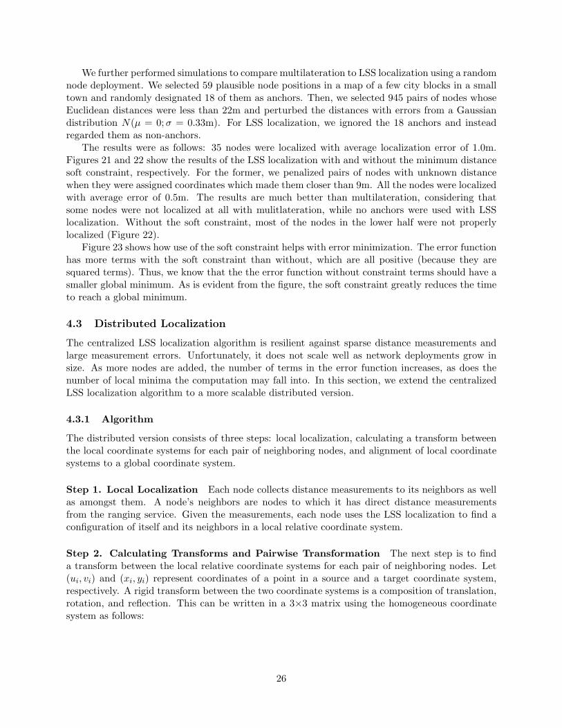
Step 2. Calculating Transforms and Pairwise Transformation The next step is to finda transform between the local relative coordinate systems for each pair of neighboring nodes. Let(ui, vi) and (xi, yi) represent coordinates of a point in a source and a target coordinate system,respectively. A rigid transform between the two coordinate systems is a composition of translation,rotation, and reflection. This can be written in a 3×3 matrix using the homogeneous coordinatesystem as follows:

26

[xn, yn, 1] = [un, vn, 1] · cos θ − sin θ 0

f sin θ f cos θ 0tx ty 1

where (tx,ty) is a translation vector, θ is a rotation angle, and f ∈ 1,−1 is a reflection factor.Calculating a transform corresponds to finding tx, ty, θ and f .

We find the transform T between two nodes a and b using their shared neighbors. Let C be theset of shared neighbors of nodes a and b which have coordinates in both local coordinate systems.A straight forward method is to use minimization. We find two solutions (θ, tx, ty, f) = argminEf ,f=1, -1, where

Ef =∑n∈C

(xn − xn,f )2 + (yn − yn,f )2

and

[xn,f , yn,f , 1] = [un, vn, 1] · cos θ − sin θ 0

f sin θ f cos θ 0tx ty 1

.

We then take the solution with the smaller error as the transform. Although this procedure returnsfairly accurate results, it is too computationally intensive to implement on resource-constrainedWSN platforms such as the MICA2 mote.

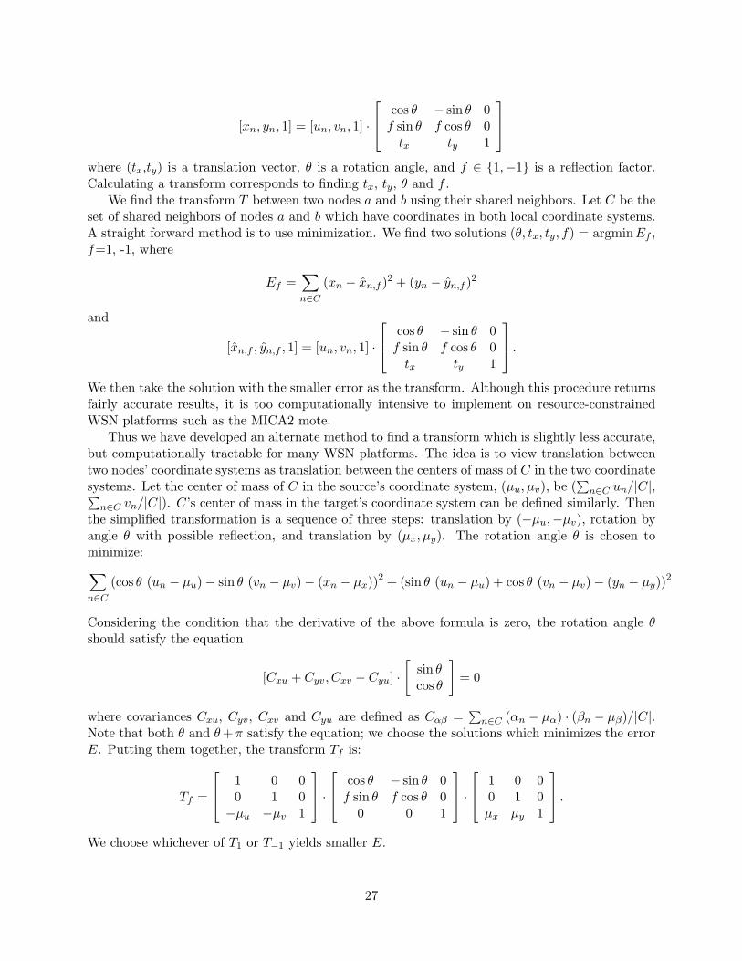
Thus we have developed an alternate method to find a transform which is slightly less accurate,but computationally tractable for many WSN platforms. The idea is to view translation betweentwo nodes’ coordinate systems as translation between the centers of mass of C in the two coordinatesystems. Let the center of mass of C in the source’s coordinate system, (µu, µv), be (

∑n∈C un/|C|,∑

n∈C vn/|C|). C’s center of mass in the target’s coordinate system can be defined similarly. Thenthe simplified transformation is a sequence of three steps: translation by (−µu,−µv), rotation byangle θ with possible reflection, and translation by (µx, µy). The rotation angle θ is chosen tominimize:∑n∈C

(cos θ (un − µu)− sin θ (vn − µv)− (xn − µx))2 + (sin θ (un − µu) + cos θ (vn − µv)− (yn − µy))2

Considering the condition that the derivative of the above formula is zero, the rotation angle θshould satisfy the equation

[Cxu + Cyv, Cxv − Cyu] ·[

sin θcos θ

]= 0

where covariances Cxu, Cyv, Cxv and Cyu are defined as Cαβ =∑

n∈C (αn − µα) · (βn − µβ)/|C|.Note that both θ and θ +π satisfy the equation; we choose the solutions which minimizes the errorE. Putting them together, the transform Tf is:

Tf =

1 0 0

0 1 0−µu −µv 1

· cos θ − sin θ 0

f sin θ f cos θ 00 0 1

· 1 0 0

0 1 0µx µy 1

.

We choose whichever of T1 or T−1 yields smaller E.

27

0

10

20

30

40

50

60

70

0 10 20 30 40 50 60

Dis

tanc

e (m

)

Distance (m)

average error: 9.494 (m)actual position

estimated position

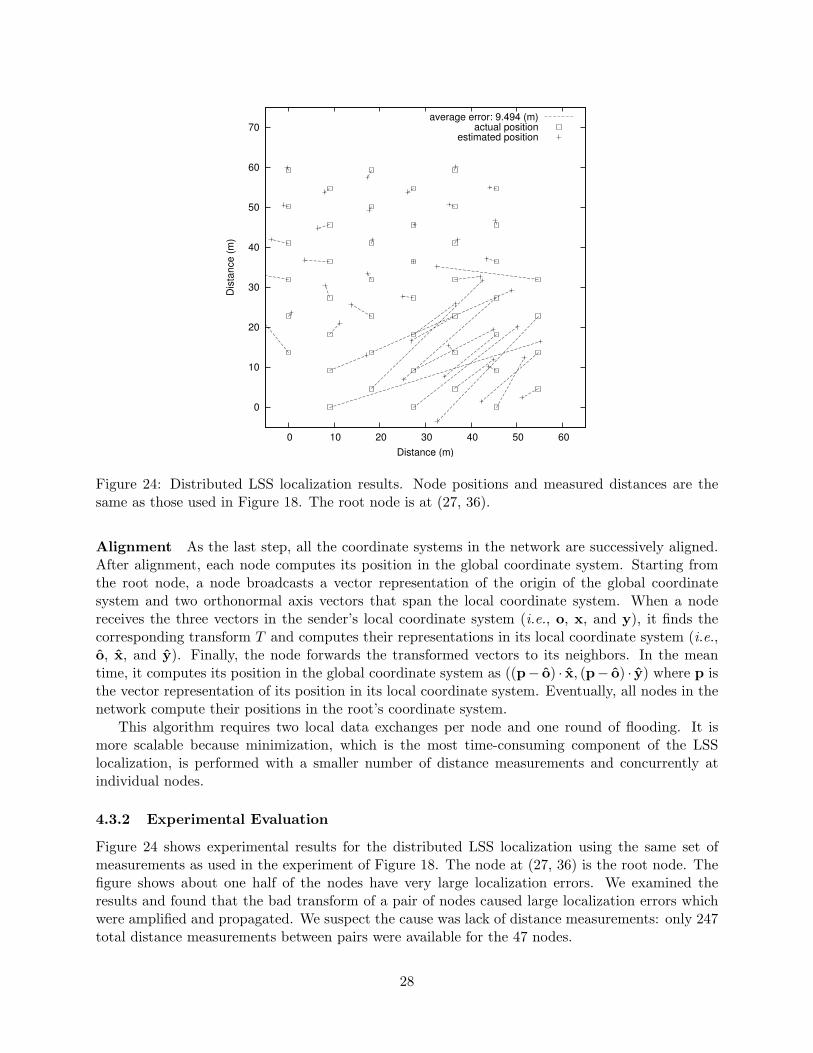
Figure 24: Distributed LSS localization results. Node positions and measured distances are thesame as those used in Figure 18. The root node is at (27, 36).

Alignment As the last step, all the coordinate systems in the network are successively aligned.After alignment, each node computes its position in the global coordinate system. Starting fromthe root node, a node broadcasts a vector representation of the origin of the global coordinatesystem and two orthonormal axis vectors that span the local coordinate system. When a nodereceives the three vectors in the sender’s local coordinate system (i.e., o, x, and y), it finds thecorresponding transform T and computes their representations in its local coordinate system (i.e.,o, x, and y). Finally, the node forwards the transformed vectors to its neighbors. In the meantime, it computes its position in the global coordinate system as ((p− o) · x, (p− o) · y) where p isthe vector representation of its position in its local coordinate system. Eventually, all nodes in thenetwork compute their positions in the root’s coordinate system.

This algorithm requires two local data exchanges per node and one round of flooding. It ismore scalable because minimization, which is the most time-consuming component of the LSSlocalization, is performed with a smaller number of distance measurements and concurrently atindividual nodes.

4.3.2 Experimental Evaluation

Figure 24 shows experimental results for the distributed LSS localization using the same set ofmeasurements as used in the experiment of Figure 18. The node at (27, 36) is the root node. Thefigure shows about one half of the nodes have very large localization errors. We examined theresults and found that the bad transform of a pair of nodes caused large localization errors whichwere amplified and propagated. We suspect the cause was lack of distance measurements: only 247total distance measurements between pairs were available for the 47 nodes.

28

0

10

20

30

40

50

60

70

0 10 20 30 40 50 60

Dis

tanc

e (m

)

Distance (m)

average error: 0.534 (m)actual position

estimated position

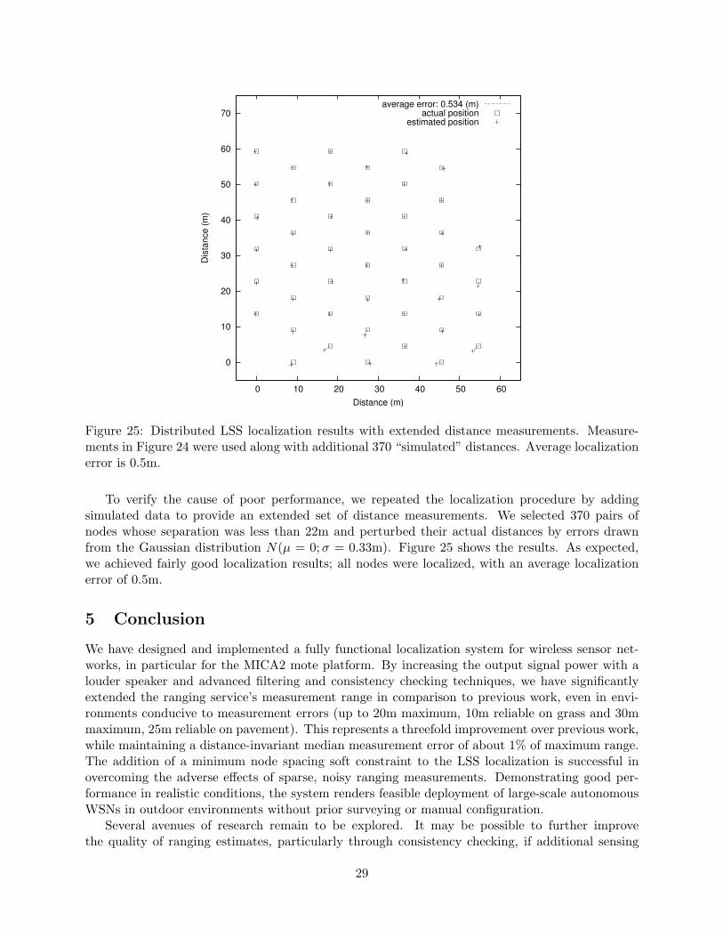
Figure 25: Distributed LSS localization results with extended distance measurements. Measure-ments in Figure 24 were used along with additional 370 “simulated” distances. Average localizationerror is 0.5m.

To verify the cause of poor performance, we repeated the localization procedure by addingsimulated data to provide an extended set of distance measurements. We selected 370 pairs ofnodes whose separation was less than 22m and perturbed their actual distances by errors drawnfrom the Gaussian distribution N(µ = 0;σ = 0.33m). Figure 25 shows the results. As expected,we achieved fairly good localization results; all nodes were localized, with an average localizationerror of 0.5m.

5 Conclusion

We have designed and implemented a fully functional localization system for wireless sensor net-works, in particular for the MICA2 mote platform. By increasing the output signal power with alouder speaker and advanced filtering and consistency checking techniques, we have significantlyextended the ranging service’s measurement range in comparison to previous work, even in envi-ronments conducive to measurement errors (up to 20m maximum, 10m reliable on grass and 30mmaximum, 25m reliable on pavement). This represents a threefold improvement over previous work,while maintaining a distance-invariant median measurement error of about 1% of maximum range.The addition of a minimum node spacing soft constraint to the LSS localization is successful inovercoming the adverse effects of sparse, noisy ranging measurements. Demonstrating good per-formance in realistic conditions, the system renders feasible deployment of large-scale autonomousWSNs in outdoor environments without prior surveying or manual configuration.

Several avenues of research remain to be explored. It may be possible to further improvethe quality of ranging estimates, particularly through consistency checking, if additional sensing

29

modalities are available to use in conjunction with acoustics. The software tone detection algorithmneeds to be extensively tested and additional improvements and optimization made before it can beused with confidence in a ranging service for WSN platforms without a hardware tone detector. Forfaster and more accurate localization, further research is necessary to fully exploit other information,such as the deployment pattern or node density. Finally, the distributed localization algorithm needsto be improved to the point where its results approach the accuracy of the centralized algorithmbefore we can reliably apply this methodology to self-localization of very large sensor networks.

Acknowledgments

This material is based upon work supported by the Defense Advanced Research Projects Agency(DARPA) under Award No. F33615-01-C-1907.

References

[1] Pierpaolo Bergamo and Gianluca Mazzini. Localization in sensor networks with fading andmobility. In Proceedings of the 13th IEEE International Symposium on Personal, Indoor, andMobile Radio Communications (PIMRC 2002), Lisboa, Portugal, September 2002.

[2] Interagency GPS Executive Board. http://www.igeb.gov/sa/.

[3] Nirupama Bulusu, John Heidemann, and Deborah Estrin. GPS-less low cost outdoor localiza-tion for very small devices. IEEE Personal Communications Magazine, 7(5):28–34, October2000.

[4] Thomas H. Cormen, Charles E. Leiserson, and Ronald L. Rivest. Introduction to Algorithms.MIT Press, 1990.

[5] Crossbow Technology, Inc. http://www.xbow.com/.

[6] Lance Doherty, Kristofer S. J. Pister, and Laurent El Ghaoui. Convex position estimation inwireless sensor networks. In Proceedings of the 20th Conference of the IEEE CommunicationsSociety (IEEE INFOCOM), pages 1655–1663, 2001.

[7] Roger Fletcher. Practical Methods of Optimization. Wiley, 1987.

[8] J. L. Hill. System Architecture for Wireless Sensor Networks. PhD thesis, University ofCalifornia, Berkeley, 2003.

[9] Bernhard Hofmann-Wellenhof, Herbert Lichtenegger, and James Collins. Global PositioningSystem: Theory and Practice. Springer-Verlag, 4th edition, 1997.

[10] Xiang Ji and Hongyuan Zha. Sensor positioning in wireless ad-hoc sensor networks withmultidimensional scaling. In Proceedings of the 23rd Conference of the IEEE CommunicationsSociety (IEEE INFOCOM), 2004. (to apear).

[11] Peter M. Lee. Multivariate Analysis: Lecture Notes. Chapter 8: Multidimensional Scaling.http://www.york.ac.uk/depts/maths/teaching/pml/mva/tex/8.ps.

[12] M. Maroti, B. Kusy, G. Simon, and A. Ledeczi. The Flooding Time Synchronization Protocol.Technical Report ISIS-04-501, Institute for Software Integrated Systems, Vanderbilt University,2004.

30

[13] Dragos Niculescu and Badri Nath. Ad hoc positioning system (APS). In GLOBECOM,November 2001.

[14] Dragos Niculescu and Badri Nath. Ad-hoc positioning system using AoA. In Proceedings ofthe IEEE/INFOCOM 2003, San Francisco, CA, April 2003.

[15] Nissanka B. Priyantha, Anit Chakraborty, and Hari Balakrishnan. The Cricket location-support system. In Mobile Computing and Networking, pages 32–43, 2000.

[16] RadioShack Corporation. 102dB Siren Sound Piezo Buzzer, Part No. 273-079.http://www.radioshack.com/.

[17] J. Sallai, G. Balogh, M. Maroti, and A. Ledeczi. Acoustic ranging in resource constrainedsensor networks. Technical Report ISIS-04-504, Institute for Software Integrated Systems,2004.

[18] Yi Shang and Wheeler Ruml. Improved MDS-based localization. In IEEE INFOCOM, 2004.

[19] Yi Shang, Wheeler Ruml, Ying Zhang, and Markus P.J. Fromherz. Localization from mereconnectivity. In Proceedings of the 4th ACM International Symposium on Mobile Ad HocNetworking & Computing, pages 201–212, Annapolis, Maryland, USA, 2003. ACM Press.http://doi.acm.org/10.1145/778415.778439.

31