Resilience assessment for interdependent urban ... · Section 4 presents the integrated asset...

1

Resilience assessment for interdependent urban 1

infrastructure systems using dynamic network flow models 2

Nils Goldbeck* 3

Centre for Transport Studies, Department of Civil and Environmental Engineering, 4

Imperial College London, Skempton Building, London SW7 2AZ, United Kingdom, 5

[email protected] 6

Panagiotis Angeloudis 7



[email protected] 10

Washington Y Ochieng 11



[email protected] 14

*Corresponding author 15

Abstract: 16

Critical infrastructure systems in cities are becoming increasingly interdependent, therefore 17

exacerbating the impacts of disruptive events through cascading failures, hindered asset repairs and 18

network congestion. Current resilience assessment methods fall short of fully capturing such 19

interdependency effects as they tend to model asset reliability and network flows separately and often 20

rely on static flow assignment methods. In this paper, we develop an integrated, dynamic modelling and 21

simulation framework that combines network and asset representations of infrastructure systems and 22

models the optimal response to disruptions using a rolling planning horizon. The framework considers 23

dependencies pertaining to failure propagation, system-of-systems architecture and resources required 24

for operating and repairing assets. Stochastic asset failure is captured by a scenario tree generation 25

algorithm whereas the redistribution of network flows and the optimal deployment of repair resources 26

are modelled using a minimum cost flow approach. A case study on London’s metro and electric power 27

networks shows how the proposed methodology can be used to assess the resilience of city-scale 28

infrastructure systems to a local flooding incident and estimate the value of the resilience loss triangle 29

for different levels of hazard exposure and repair capabilities. 30

Keywords: Resilience assessment, interdependent infrastructure systems, infrastructure assets, 31

repairable systems modelling, dynamic network flow modelling 32

2

1. INTRODUCTION 1

Various disasters in recent years have brought to light critical infrastructure vulnerabilities linked to 2

interactions between different systems. For example, the disruptions caused by superstorm Sandy in 3

New York City in 2012 were aggravated by various incidents of cascading failure [1]. Extensive power 4

outages made it more difficult to remove flood water from metro tunnels [2]. The liquid fuel supply 5

chain broke down due to direct flood damage to terminals, refineries and pipelines, combined with 6

power outages and traffic restrictions on the waterways [3]. The fuel shortage, in turn, affected 7

emergency response services and efforts to restore power supply. Similar interactions have been 8

documented for other disasters, including the 1998 ice storm in Canada [4], 2008 winter storms in 9

China [5], 2010 earthquake in Chile [6], and 2010/2011 earthquakes in New Zealand [7]. 10

The interplay of different infrastructure systems can equally exacerbate impacts of much smaller 11

trigger events. In 2015, a fire started in an underground electrical substation in London and damaged a 12

natural gas pipeline, which in turn fuelled the fire for 36 hours [8]. Despite being a relatively local 13

incident, it resulted in high costs for businesses due to disruptions in power, communication and 14

transport systems. 15

These examples demonstrate that the state of a critical infrastructure system can be affected by 16

disruptions in other systems through different types of dependency relations. Systems that are mutually 17

dependent on each other are referred to as interdependent infrastructure systems or a system-of-systems. 18

Rinaldi et al. [9] were among the first to highlight the trend of increasing infrastructure interdependency 19

and expressed concern that assessing the performance of each system separately could be misleading 20

because important interdependency effects are not taken into account. The issue has since gained the 21

attention of many researchers, government authorities and industry practitioners, especially in 22

conjunction with the emerging concept of infrastructure resilience. 23

Traditional risk management strategies provide plans to avoid, control, transfer or assume risks based 24

on assessing their probability and impact. The applicability of such methods is limited when there is 25

high uncertainty regarding the risk matrix and effectiveness of control or avoidance measures. This is 26

increasingly the case for urban infrastructure systems, and the concept of infrastructure resilience 27

extends risk management efforts accordingly. Infrastructure resilience describes the ability of systems 28

to resist, recover and adapt in order to maintain their core function after a perturbation (for a 29

comprehensive review of definitions see [10]). As such, resilience approaches seek to understand the 30

dynamic behaviour of systems on different timescales and optimise both preparedness and recovery 31

capabilities. As this dynamic behaviour is increasingly determined by interdependencies, new methods 32

are needed to model urban infrastructure as a system-of-systems and carry out comprehensive resilience 33

assessments. 34

Qualitative studies in this field have provided definitions and typologies of infrastructure 35

dependencies (e.g. [9], [11], [12]). Several quantitative methods have been developed or adapted to 36

3

analyse the resilience of interdependent infrastructure systems, including fault tree analysis [13], system 1

dynamics [14], agent-based simulation [15], input-output modelling [16], and network modelling [17]–2

[24]. Comprehensive reviews of such methods are provided by Ouyang [25] and Iturriza et al. [26]. 3

Regarding priorities for future research, Ouyang [25] and Zio [27] highlight the importance of model 4

integration and co-simulation. 5

Modelling approaches using network science broadly fall into two categories: topological models 6

and flow models. Topological models (e.g. [17], [19], [21], [24]) show that interdependencies are a 7

source of additional vulnerabilities and can aid network collapse. However, topological models only 8

analyse network structure and fail to capture fundamental aspects of infrastructure networks beyond 9

connectivity, for example, partial capacity loss, routing and congestion. Previous studies have shown 10

that more realistic vulnerability and resilience assessments can be achieved with network flow models, 11

which seek to predict the flow of passengers, goods, power or information, taking into account the 12

capacity of different network components and other operational network characteristics [28]–[32]. The 13

network flow models proposed by Lee II et al. [18], Holden et al. [20], Jin et al. [22] and Fotouhi et 14

al. [23] are particularly relevant to this paper, given their ability to capture interdependent networks. 15

Key features of these models are presented in Table 1. 16

Table 1 Key features of network flow models for interdependent urban infrastructure systems 17

Lee II et al. [18]

Holden et al. [20]

Jin et al. [22]

Fotouhi et al. [23]

Case study area New York City n.a. Singapore Minneapolis

Networks considered Metro

Electric power

Telephone

Water

Electric power

Metro

Bus

Road

Electric power

Single-commodity networks ()

Multi-commodity networks

Network size 100 - 1000 nodes 6 nodes 77 nodes 8 nodes

Resilience measure Total cost (incl. penalty for unmet

demand)

Satisfied demand Satisfied demand Total travel time

Min. cost flow assignment

Dynamic flows

Coupling of flows

Partial capacity loss continuous discrete

Mitigation Temporary power and telephone connections

Replacement bus services

Backup power supply, traffic regulation by police officers

Repair

Integer variables

Nonlinear constraints

Stochastic optimisation

18

A common feature found across most state-of-the-art network flow models is their use of minimum 19

cost flow methods to assign flows to capacitated networks, with differences in the representation of 20

flow relationships between different networks. For instance, Holden et al. [20] use a linear production 21

4

function that defines the quantities of input resources required for the production of another good. 1

Fotouhi et al. [23] add delays to road links if traffic signals fail, depending on whether the junctions are 2

subsequently unregulated or regulated manually by police officers. While such modelling techniques 3

achieve tailor-made solutions to capture specific aspects of infrastructure systems, a more generic 4

approach is needed that can represent the many different interactions between network flows and 5

physical infrastructure assets. 6

In existing network flow models, infrastructure assets, such as metro stations, railway tracks or 7

electricity substations, are often modelled as simple nodes or links whose operational characteristics are 8

condensed into one-dimensional operability variables. Moreover, these operability variables are usually 9

exogenous or subject to a simple stochastic process (random failure). In reality, such infrastructure 10

assets are complex systems themselves, consisting of sub-systems and components. The realism of 11

network flow models could be improved by modelling the multi-level architecture of infrastructure 12

assets, for example using the reliability engineering concept of series and parallel systems. 13

With recovery time being a core resilience dimension, resilience assessment methods are required 14

to model the dynamic behaviour of interdependent infrastructure systems. The two-stage stochastic 15

programming methods proposed in Jin et al. [22] and Fotouhi et al. [23] consider decisions taken at two 16

points in time (before and after the disruption), but the actual flow assignment is static. In Holden et 17

al. [20], the static flow assignment is repeated over a series of time steps. However, none of the reviewed 18

models features a dynamic flow assignment where flows can span over multiple time steps. Moreover, 19

there exists currently no models that capture the dynamic interplay of network flows and asset 20

operability during the recovery period. 21

The optimisation problems in the reviewed models are either inherently linear or linearly 22

approximated. However, they often include binary variables and, therefore, belong to the class of NP-23

hard computational problems. We note that most case studies presented in the literature involve network 24

instances featuring fewer than 100 nodes, with the exception of the New York City example in Lee II 25

et al. [18]. City-scale infrastructure networks are at least one order of magnitude larger. While in some 26

cases it may be practical to assess or optimise resilience considering only a smaller local area, there is 27

also a need for models that are scalable to full-size urban infrastructure networks. 28

Summarising, this paper seeks to address three gaps in the literature: i) lack of methods to represent 29

infrastructure assets in network flow models more realistically and capture the relationship between 30

network flows and asset operability, ii) insufficient modelling of dynamic effects during the recovery 31

period, and iii) limited scalability. The remainder of the paper is structured as follows. Section 2 presents 32

resilience measures. Section 3 introduces the modelling framework, including four types of dependency 33

relations. Section 4 presents the integrated asset operability and network flow model. The application 34

of the method is demonstrated in a case study on London in Section 5. 35

5

Table 2 Nomenclature 1

Sets Parameters Variables

𝐴 Infrastructure assets 𝑡max Number of simulation timesteps

𝑍𝑘,𝑚𝑡

Random variable for failure propagation

𝐴S Series systems assets 𝑡ph Length of the planning horizon

𝑧𝑘𝑡 Asset failure variable for 𝑘

𝐴P Parallel systems assets 𝑛scn Max. number scenarios 𝑥𝑘𝑡 Operability of asset 𝑘

𝐻 Hazard events 𝑛spl Number of samples per scenario tree node

𝑦𝑘𝑡 Utilisation of asset 𝑘

𝑉SC Nodes in single-commodity systems

𝑘 Number of shortest paths per OD pair

𝑓𝑖,𝑗 𝑡 Flow on link (𝑖, 𝑗)

𝑉MC Nodes in multi-commodity systems

�̌�𝑖𝑡

Commodity demand at node 𝑖

𝑓𝑝𝑡 Flow on path 𝑝

𝐸SC Links in single-commodity systems

𝑓𝑜,𝑑𝑡 Travel demand from 𝑜 to 𝑑 𝑔𝑖

𝑡 Commodity generation at node 𝑖

𝐸MC Links in multi-commodity systems

𝑣𝑖SC

Value of commodity demand at node 𝑖

𝑢𝑖𝑡

Commodity delivery at node 𝑖

𝑂𝐷 OD pairs 𝑣𝑜,𝑑MC

Value of travel demand from 𝑜 to d

VoD𝑡 Value of demand

𝑃𝑜,𝑑 Shortest paths from 𝑜 to 𝑑 𝑓𝑖,𝑗 Capacity of link (𝑖, 𝑗) VoS𝑡 Value of supply

𝑄𝑖,𝑗 Paths using link (𝑖, 𝑗) �̂�𝑖 Capacity of node 𝑖 RLT Area of the resilience loss triangle

𝐷F Failure propagation dependencies

𝑐𝑖,𝑗f Cost of flow on link (𝑖, 𝑗) MSP

Minimum system performance

𝐷L Logic dependencies 𝑐𝑖g

Cost of commodity generation at node 𝑖

TLD Total length of disruption

𝐷U Asset utilisation dependencies

𝑝𝑘,𝑚 Probability of failure propagation from 𝑘 to 𝑚

𝐷I Resource input dependencies

𝑡𝑘,𝑚 Time lag of failure propagation from 𝑘 to 𝑚

𝛼𝑖,𝑘U

Resources provided by 𝑖 for the utilisation of 𝑘

𝛼𝑖,𝑘R

Resources provided by 𝑖 for the repair of 𝑘

2

6

2. RESILIENCE MEASURES 1

Literature reviews by Hosseini et al. [10] and Sun et al. [33] highlight the existence of several 2

competing measures of infrastructure resilience. One of the most commonly used approaches is the loss 3

triangle method, which quantifies resilience based on the loss of system performance integrated over 4

the time it takes for the system to recover after a disruption [34]. 5

Performance measures used in this context include those that are based on asset operability (e.g. [15], 6

[31], [32], [35]), network connectivity (e.g. [17], [36]–[39]), network capacity (e.g. [40], [41]), satisfied 7

demand (e.g. [15], [22], [24], [31], [32], [42]–[44]), and the value of services provided (e.g. [23], [45]–8

[50]). In this paper, we use a performance measure based on the value of service provision because it 9

has the following advantages: First, a value-based performance measure is most relevant from a societal 10

perspective, as it captures the quantity and quality of services provided by infrastructure systems to 11

meet a certain demand. Second, it can usually be expressed in monetary values, which facilitates the 12

aggregation of performance measures for different infrastructure systems and services. Third, positive 13

and negative externalities can be integrated in the performance measure by converting them to monetary 14

values. The difficulty of using a value-based performance measure is that more sophisticated prediction 15

models and data inputs are required for its evaluation compared to other performance measures. 16

We propose a generic performance measure that can be applied to all types of infrastructure systems. 17

Services provided by these systems are of two types: i) the supply of a homogeneous good or service to 18

a set of demand nodes, or ii) the transportation of inhomogeneous goods, passengers or information 19

between origin-destination (OD) pairs. Distinguishing these two types of infrastructure services is 20

important because they require different flow assignment methods, referred to as single- and multi-21

commodity network assignment. 22

An overview of the notation used throughout this paper is provided in Table 2. The demand for 23

infrastructure services is assumed to be given by parameters �̌�𝑖𝑡 for goods or services required at nodes 24

𝑖 ∈ 𝑉SC in single-commodity networks and 𝑓𝑜,𝑑𝑡 for transportation services between two nodes (𝑜, 𝑑) ∈25

𝑂𝐷 in multi-commodity networks. In the first instance, our model does not capture demand elasticity, 26

but the framework could be extended in this respect in the future. 27

We assume that the monetary value of fulfilling one unit of the demand for infrastructure services 28

with a standard quality of service level can be estimated by parameters 𝑣𝑖SC and 𝑣𝑜,𝑑

MC. The total value of 29

demand (VoD) at time step 𝑡 can then be calculated as follows: 30

VoD𝑡 = ∑ 𝑣𝑖SC�̌�𝑖

𝑡

𝑖∈𝑉SC

+ ∑ 𝑣𝑜,𝑑MC𝑓𝑜,𝑑

𝑡

(𝑜,𝑑)∈𝑂𝐷

(1)

31

7

When a disruption occurs, it is possible that some of the demand remains unsatisfied. Additionally, 1

there could be a deterioration of service quality. The value of supply (VoS) is calculated as follows: 2

VoS𝑡 = ∑ 𝛼𝑖𝑡𝑣𝑖

SC𝑢𝑖𝑡

𝑖∈𝑉SC

+ ∑ 𝑣𝑜,𝑑MC ∑

𝑐𝑜,𝑑

𝑐𝑝𝑓𝑝

𝑡

𝑝∈𝑃𝑜,𝑑(𝑜,𝑑)∈𝑂𝐷

(2)

For a single-commodity node 𝑖 ∈ 𝑉SC, the value of supply is the quantity supplied 𝑢𝑖𝑡, multiplied by 3

the value of delivering this commodity 𝑣𝑖SC, and a discount factor 𝛼𝑖

𝑡 ∈ [0,1] indicating the quality of 4

service. Similarly, for an origin destination pair (𝑜, 𝑑) ∈ 𝑂𝐷, the discount factor applied to path flows 5

𝑓𝑝𝑡 is

𝑐𝑜,𝑑

𝑐𝑝 , where 𝑐𝑜,𝑑 and 𝑐𝑝 are the generalised costs of transport between 𝑜 and 𝑑 over the shortest 6

path and over the chosen path 𝑝 respectively. 7

With the overall system performance measure VoS𝑡

VoD𝑡 , we can now calculate the main resilience 8

measure, the area of the resilience loss triangle (RLT), by integrating over all simulation time steps: 9

RLT = ∑ (1 −VoS𝑡

VoD𝑡)

𝑡max

𝑡=0

(3)

Two additional measures are used to capture aspects which other studies describe as the robustness 10

and rapidity dimensions of resilience [51]. Robustness can be seen as the minimum system performance: 11

MSP = min𝑡=0,…,𝑡max

(1 −VoS𝑡

VoD𝑡) (4)

The rapidity of recovery is measured by the total length of the disruptions, i.e. the number of time 12

steps where the system performance is less than one: 13

TLD = ∑ 𝟙{𝑥<1} (VoS𝑡

VoD𝑡)

𝑡max

𝑡=0

(5)

Note that the resilience measures formulated above do not include the costs of infrastructure service 14

provision, which are likely to increase after a disruptive event due to recovery and repair costs. 15

Furthermore, externalities may occur, such as environmental impacts. The network flow modelling 16

method can capture these costs by adding them either to the objective function (e.g. monetised 17

environmental impacts) or as constraints (e.g. repair budgets). 18

8

3. METHODOLOGICAL FRAMEWORK 1

In this section, we present a modelling and simulation framework that can be used to assess the 2

resilience of a system of interdependent infrastructure systems. Figure 1 presents the high-level 3

architecture and the remainder of this section describes how the model represents infrastructure systems 4

and dependency relations. 5

6

Figure 1 Overview of the modelling framework 7

3.1. Infrastructure systems 8

We represent infrastructure systems as networks (consisting of nodes and directed links) that are 9

inter-connected with physical or non-physical assets. The network representation models the services 10

provided by infrastructure systems. The asset representation models system components required for 11

providing these services and their exposure to hazards. 12

Separating the network and asset representation enables us to extend the scope of the model with 13

respect to network and asset effects independently of each other. Consider the example of a metro 14

station. In the simplest case, it can be represented using one node and one asset. Network characteristics 15

(i.e. the station’s usage by passengers) could be modelled with greater detail by representing entrances, 16

exits and platforms as separate nodes. Asset characteristics (i.e. the failure and repair of different 17

components) could be modelled with greater detail by representing escalators, ventilation and lighting 18

as separate sub-assets. There is no limit to increasing the level of detail by adding additional components 19

to the asset and network mapping. 20

Assets can represent specific pieces of equipment (e.g. electricity transformers), buildings (e.g. 21

metro stations or tunnels) or entire sub-systems (e.g. train control systems). Their operability is 22

described by continuous variables x𝑘𝑡 ∈ [0,1]. The occurrence of a hazard event or the propagation of 23

Assets &

hazards

Nodes &

links

Stochastic failure

propagation

dependencies

Origin

destination

pairs

Shortest path

estimation

Asset failure

scenario generation

Dynamic network flow model

Asset utilisation

dependencies

Logic

dependencies

Input

requirement

dependencies

Single- and

multi-commodity

demand

Expected system-

of-systems

performance

Time

100 %

50 %

th tr

RLT

TLD

MSP

for t = 0 … tmax:

for each scenario tree node:

Optimise

• repair resource deployment

• asset repair rates

• commodity production

• link and path flows

over the current planning horizon

tmax

9

failure among interdependent assets can cause assets to fail, which would be represented by assigning 1

the operability variables of affected components to x𝑘𝑡 = 0. To regain their operability, assets require 2

repair. 3

The network and asset representations of infrastructure systems are interdependent in the sense that 4

network flows may require the utilisation of assets and the utilisation and repair of assets may require 5

resources provided by networks. All inter- and intra-system dependencies are represented by directed 6

dependency relations between nodes, links and assets. 7

3.2. Dependency relations 8

Several types of dependency relations have been identified in the literature. For example, Rinaldi et 9

al. [9] define physical, cyber, geographic and logic dependencies. Zimmerman [11] distinguishes 10

between functional and spatial dependencies. Dudenhoeffer et al. [12] describe physical, informational, 11

geospatial, procedural and societal dependencies. A common characteristic of these typologies is their 12

focus on the underlying cause of a dependency. This approach is useful for identifying and mapping 13

dependencies. As far as modelling dependencies is concerned, we deem their effects as more important 14

than their cause. Dependencies can have similar effects despite having different causes, or vice versa. 15

Consider, for example, the physical and cyber dependencies proposed by Rinaldi et al. [9], describing 16

dependencies on material inputs from or information transmitted through another network. From a 17

network flow modelling perspective, there is no fundamental difference between them, because in both 18

cases a disruption of flows in the network supplying a service would disrupt flows in the dependent 19

network. 20

In this paper, we propose a new, effect-based classification of dependency relations into four types: 21

i) stochastic failure propagation, ii) logic, iii) asset utilisation, and iv) resource input dependencies. 22

Figure 2 presents a simple example of two interdependent systems, which we will use in the following 23

sub-sections to introduce how these dependencies are modelled. 24

25

Figure 2 System representation and dependency types 26

N1 N2 N3 N4

A1 A2 A3

A4 A5

N5 N7

A6

N6

Asset utilisation

dependencies

1 1 1

1

1

Logic dependencies2

2

Resource input

dependencies3

Failure propagation

dependencies4

334

Node Link

Asset

System 1

System 2

Network

layer

Asset

layer

Asset

layer

Network

layer

Dependency type: Possible cause:

System architecture,

network topology

Series or parallel

system configuration

Physical inputs,

cyber dependencies

Spatial proximity, chain

of cause and effect

Dependency

H1

Hazard

4

10

3.2.1. Stochastic failure propagation dependencies 1

Failure propagation dependencies relate to geographic, spatial or co-location dependencies in cause-2

based typologies. They essentially describe a correlation between the failure probabilities of two assets, 3

which could be the result of direct causation (e.g. the failure of a bridge damages railway tracks 4

underneath it) or a shared hazard exposure (e.g. cables in a shared utility trench). Our modelling 5

framework captuers failure propagation by considering an asset’s failure probability a conditional 6

probability depending on the occurance of hazard events and failure of other assets. 7

The example in Figure 2 contains five failure propagation dependencies, ultimately linked to a 8

hazard H1 that affects assets A5 and A6. Due to spatial proximity, the failure of either one of these 9

assets increases the probability that the other fails, which is represented by two directed failure 10

propagation dependencies between them. If A5 fails, the failure can further propagate to A3. 11

Failure propagation dependencies are contained in the set 𝐷F and specify the probability and time 12

lag with which failures can propagate. For simplicity, we assume that there is no uncertainty regarding 13

the time lag. Thus, each dependency relation (𝑘, 𝑚) ∈ 𝐷F is described by two parameters: the 14

probability of failure propagation 𝑝𝑘,𝑚 and time lag 𝑡𝑘,𝑚. 15

For every failure propagation dependency and every time step of the simulation period, the model 16

contains a binary random variable 𝑍𝑘,𝑚𝑡 that indicates whether the dependency is active (𝑍𝑘,𝑚

𝑡 = 1) or 17

not (𝑍𝑘,𝑚𝑡 = 0) . These random variables are independent and Bernoulli distributed with Pr(𝑍𝑘,𝑚

𝑡 =18

1) = 𝑝𝑘,𝑚. If 𝑘 is a hazard that is active at time 𝑡 or an asset that fails at time 𝑡 the failure spreads to 19

the assets contained in the set {𝑚: (𝑘, 𝑚) ∈ 𝐷F and 𝑍𝑘,𝑚𝑡 = 1}. 20

Note that the model considers only one type of failure per asset. In cases where it is required to 21

capture different failure modes, an asset is decomposed into sub-assets according to a fault tree analysis. 22

Each sub-asset has its own failure mode and they are connected through logic dependencies. 23

3.2.2. Logic dependencies 24

We distinguish series system assets (contained in the sub-set 𝐴S ) and parallel system assets 25

(contained in the sub-set 𝐴P). For example, asset A2 in Figure 2 could represent a metro line modelled 26

as a series system asset that requires the train control system (A4) and the railway track (A5) to be 27

operational. The model could be extended by assuming that the train control system is a parallel system 28

asset depending on two redundant control centres which would be added as sub-assets of A4. 29

11

The hierarchy of assets and sub-assets is captured by logic dependency relations contained in the 1

set 𝐷L . In contrast to failure propagation dependencies, we consider logic dependencies to be 2

deterministic and have immediate effects. The operability of series system assets is constrained by the 3

minimum operability of all assets that they depend on via a logic dependency relation: 4

xk𝑡 ≤ 𝑥𝑚

𝑡 𝑘 ∈ 𝐴S, (𝑚, 𝑘) ∈ 𝐷L, 𝑡 = 0, … , 𝑡max (6)

The operability of parallel system assets is constrained by the following equation: 5

𝑥𝑘𝑡 ≤ ∑ 𝑥𝑚

𝑡

(𝑚,𝑘)∈𝐷L

𝑘 ∈ 𝐴P, 𝑡 = 0, … , 𝑡max (7)

This implies the assumption that the maximum operability of parallel system assets is a linear 6

combination of the sub-systems’ operabilities. 7

3.2.3. Asset utilisation dependencies 8

Asset utilisation dependencies are contained in the set 𝐷U and connect the asset to the network 9

representation in our modelling framework. Our toy model in Figure 2 contains seven asset utilisation 10

dependencies, for example asset A1 is used by the two links (N1, N2) and (N2, N1), and asset A6 is 11

used by the supply node N6. 12

We introduce asset utilisation variables 𝑦𝑘𝑡 ∈ [0,1] that are defined as the maximum capacity 13

utilisation of all nodes and links depending on an asset. In the model, this is captured by inequality 14

constraints 15

1

𝑓𝑖,𝑗

𝑓i,j𝑡 ≤ 𝑦𝑘

𝑡 𝑘 ∈ 𝐴, (𝑘, (𝑖, 𝑗)) ∈ 𝐷U , 𝑡 = 0, … , 𝑡max (8)

1

�̂�𝑖 𝑔i

𝑡 ≤ 𝑦𝑘𝑡 𝑘 ∈ 𝐴, (𝑘, 𝑖) ∈ 𝐷U, 𝑡 = 0, … , 𝑡max (9)

where 𝑓i,j𝑡 and 𝑔i

𝑡 denote the current link flow and commodity generation at a dependent link or node 16

respectively, and 𝑓𝑖,𝑗 and 𝑔𝑖 denote the flow and generation capacities. 17

Asset utilisation dependencies have two effects. Firstly, if an asset fails and becomes inoperable the 18

generation or transmission capacities of dependent nodes and links are reduced accordingly until the 19

asset is repaired. This can be modelled by constraining the asset utilisation variable to be less than or 20

equal to the asset operability variable: 21

𝑦𝑘𝑡 ≤ 𝑥𝑘

𝑡 𝑘 ∈ 𝐴, 𝑡 = 0, … , 𝑡max (10)

The second effect of asset utilisation dependencies occurs in conjunction with resource input 22

dependencies. 23

12

3.2.4. Resource input dependencies 1

Resource input dependencies contained in the set 𝐷I also form a link between the two layers of the 2

modelling framework, but in the opposite direction as asset utilisation dependencies. In the example in 3

Figure 2, System 2 provides a resource to System 1, modelled by resource input dependencies (N5, A1) 4

and (N7, A3). 5

The quantity of a resource input from node 𝑖 to asset 𝑘 is assumed to be proportional to the asset 6

utilisation 𝑦𝑘𝑡 with parameter 𝛼𝑖,𝑘

U and to the asset repair rate (𝑥𝑘𝑡+1 − 𝑥𝑘

𝑡 ) with parameter 𝛼𝑖,𝑘R . The total 7

amount of resources supplied by 𝑖 in time step 𝑡 to all assets that depend on it can be calculated as 8

follows: 9

∑ (𝛼𝑖,𝑘U 𝑦𝑘

𝑡 + 𝛼𝑖,𝑘R (𝑥𝑘

𝑡+1 − 𝑥𝑘𝑡 ))

𝑘∈𝐴:(𝑖,𝑘)∈𝐷I

(11)

In the case of supply shortages, resource input dependencies have the effect that the utilisation of an 10

asset has to be reduced and / or its repair deferred until sufficient resources are available. 11

13

4. INTEGRATED ASSET OPERABILITY AND NETWORK FLOW MODEL 1

This section presents an integrated asset operability and network flow model that implements the 2

modelling principles described above. Key elements of the methodology are a stochastic asset failure 3

model, a scenario tree generation algorithm and a minimum cost flow assignment model. 4

4.1. Time-expanded asset-hazard graph 5

A hazard ℎ ∈ 𝐻 in our model is assumed to occur at a specific time 𝑡ℎ. The uncertainty in the model 6

stems from the stochastic failure propagation dependencies (𝑘, 𝑚) ∈ 𝐷F, which can be active (𝑍𝑘,𝑚𝑡 =7

1) or inactive (𝑍𝑘,𝑚𝑡 = 0). Given a sample of active failure propagation dependencies, we can create the 8

time-expanded asset-hazard graph 𝐺AH, whose node set is 𝐴 ∪ 𝐻 expanded over time steps 0, … , 𝑡max. 9

The link set contains the active failure propagation dependencies. Figure 3 depicts an asset-hazard graph 10

for the example introduced in Figure 2. The graph visualises that in this specific sample the direct impact 11

of the hazard event at 𝑡ℎ = 1 is the failure of asset A5 at 𝑡 = 2. The second order impacts are the failures 12

of A5 in the same time step and A3 at 𝑡 = 3. 13

14

Figure 3 Time-expanded asset-hazard graph for the example in Figure 2 15

Let the variables 𝑧𝑘𝑡 indicate whether an asset 𝑘 ∈ 𝐴 fails (𝑧𝑘

𝑡 = 1) or not (𝑧𝑘𝑡 = 0) at time 𝑡. Given 16

a sample of failure propagation variables {𝑍𝑘,𝑚𝑡 , : (𝑘, 𝑚) ∈ 𝐷F} we can derive the asset failure variables 17

{𝑧𝑘𝑡 : 𝑘 ∈ 𝐴} by constructing the asset-hazard graph and testing which nodes can be reached from an 18

active hazard: 19

𝑧𝑘𝑡 = {

1 if (𝑘, 𝑡) can be reached from any (ℎ, 𝑡ℎ), ℎ ∈ 𝐻0 otherwise

𝑘 ∈ 𝐴, 𝑡 = 0, … , 𝑡max (12)

Asset failures that are separated by only one failure propagation dependency from the hazard node 20

are failures that occur as a direct impact of the hazard. Failures that are separated by more than one 21

dependency can be considered as higher-order cascading failure effects. 22

Hazard 1

Asset 3

Asset 5

Asset 6

t = 0 t = 1 t = 2 t = 3 t = 4

Inactive failure propagation dependency

Active failure propagation dependency

Hazard event

Asset failure

14

4.2. Scenario tree generation 1

A simple way of integrating the stochastic asset failure model and flow assignment would be to 2

create a number of asset failure samples and then carry out the network flow assignment for each 3

scenario independently. Using such an approach, the flow assignment would have to be computed for 4

𝑛scn × 𝑡max time steps, where 𝑛scn denotes the number of scenarios. This would be computationally 5

inefficient because the flow assignment computations would be redundant for the period before the first 6

hazard event, in which all asset failure scenarios are identical. 7

A more efficient model integration approach is to generate a scenario tree, taking advantage of the 8

fact that asset failure scenarios gradually diverge over time due to the uncertainty of failure propagation. 9

Assuming that the first hazard occurs at 𝑡ℎ and the scenario tree immediately diverges from one to 𝑛scn 10

branches, the number of time steps for which the flow assignment has to be solved reduces to 𝑡ℎ +11

𝑛scn(𝑡max − 𝑡ℎ) . In the average case, where divergence is slower, the number of necessary flow 12

assignment computations is even lower. 13

The method used to generate a scenario tree is presented in Algorithm 1, which uses two parameters 14

to control branching. Firstly, 𝑛spl is the number of samples generated for each scenario tree node to 15

populate the set of possible child nodes 𝑆children. A higher value of 𝑛spl would increase the rate of tree 16

branching and capture a wider range of possible failure propagation. Moreover, it would increase the 17

accuracy of the probability distribution over 𝑆children, which is calculated as the number of times each 18

sample value is observed divided by 𝑛spl. 19

Tree branching is restricted by the second parameter 𝑛scn in order to ensure that a maximum number 20

of final scenarios is not exceeded and that the branching is distributed equally among all existing 21

branches. The maximum number of child nodes added to the tree is 22

⌈𝑛scn − |𝑆𝑡−1|

|𝑆𝑡−1|⌉ (13)

where 𝑆𝑡−1 is the set of scenario tree nodes in time step 𝑡 − 1. If the number of unique samples obtained 23

from the stochastic asset failure model is greater than the value in (13), the required number of samples 24

is selected randomly from the samples generated and the scenario probabilities are re-normalised. 25

15

Algorithm 1 Scenario tree generation 1

Algorithm ScenarioTreeGeneration

1 Input: Set of assets 𝐴, set of hazards 𝐻

2 Set of failure propagation dependencies 𝐷FP

3 Maximum number of scenarios 𝑛scn, Number of samples per parent node 𝑛spl

4 Number of simulation time steps 𝑡max

5 Output: Scenario tree 𝑆

6 Initialise 𝑆𝑡 = { } for 𝑡 = 0, … , 𝑡max

7 New scenario tree node 𝑠root

8 Probability(𝑠root) ← 1

9 AssetFailure(𝑠root) ← {𝑧𝑘0 = 0, 𝑘 ∈ 𝐴}

10 Add 𝑠root to 𝑆0

11 For 𝑡 = 1, … , 𝑡max

12 For each 𝑠parent in 𝑆𝑡−1

13 𝑆children = { }

14 For 𝑖 = 1, … , 𝑛spl

15 New scenario tree node 𝑠sample

16 Parent(𝑠sample) ← 𝑠𝑝𝑎𝑟𝑒𝑛𝑡

17 Probability(𝑠sample) ← Probability(𝑠parent) / 𝑛spl

18 Sample failure propagation variables 𝑍𝑘,𝑚𝑡 and create asset hazard graph

19 AssetFailure(𝑠sample) ← {𝑧𝑘𝑡 = {

1 if (𝑘, 𝑡) is reachable from any (ℎ, 𝑡ℎ), ℎ ∈ 𝐻0 otherwise

, 𝑘 ∈ 𝐴}

20 If 𝑆𝑡 contains any 𝑠ident where AssetFailure(𝑠ident) == AssetFailure(𝑠sample)

21 Probability(𝑠ident) ← Probability(𝑠ident) + Probability(𝑠sample)

22 Else

23 Add 𝑠sample to 𝑆children

24 If |𝑆children| > ⌈𝑛scn−|𝑆𝑡−1|

|𝑆𝑡−1|⌉

25 Randomly discard |𝑆children| − ⌈𝑛scn−|𝑆𝑡−1|

|𝑆𝑡−1|⌉ child nodes from 𝑆children

26 Normalise probabilities in 𝑆children

27 Add 𝑆children to 𝑆𝑡

28 Return 𝑆 = [𝑆0, 𝑆1, … , 𝑆𝑇]

2

4.3. Dynamic network flow model 3

The dynamic network flow model used in this paper is based on a minimum cost flow assignment 4

method, deployed in a rolling planning horizon framework and extended with three types of dependency 5

relations (asset utilisation, resource input, logic) and the optimisation of asset repair. 6

4.3.1. Rolling planning horizon 7

Holden et al. [20] model dynamic flows by solving a separate minimum cost flow problem for each 8

time step. However, this technique cannot model flows with a duration greater than the length of one 9

time step and does not allow foresight and planning. The latter point is particularly relevant for models 10

with repairable systems and limited repair capacity because optimal repair strategies have to anticipate 11

where network capacity is most needed in order to prioritise repair. These limitations can be overcome 12

by transforming the network into a time-expanded network [52]. However, with this technique the size 13

of the resulting optimisation problem increases linearly with the number of time steps, limiting the 14

16

scalability of the method. Moreover, the transformation into a single optimisation problem for all time 1

steps means that the model assumes perfect foresight, which is arguably as unrealistic as the assumption 2

of no foresight. While it is realistic that system operators anticipate the results of their own actions, such 3

as repair measures, it is unrealistic that they can fully anticipate random events, such as equipment 4

failure. 5

The model presented in this paper combines the iterative and time-expanded network approaches by 6

using a rolling planning horizon with a length of 𝑡ph time steps. Iterating the current time step 𝑡c 7

through the simulation period 0, … , 𝑡max, a time-expanded network flow problem is solved for each 8

planning horizon 𝑡c, … , 𝑡c + 𝑡ph. However, only the optimal values of the decision variables for the first 9

time step of each planning horizon are saved as simulation results. The flows computed for time steps 10

𝑡c + 1, … , 𝑡c + 𝑡ph indicate what is anticipated at time 𝑡c. These predictions are updated in subsequent 11

iterations and the final value of a decision variable is obtained when its respective time step becomes 12

the current time step. 13

Combining the iterative and time-expanded network approaches has two important advantages. 14

Firstly, it limits the size of the optimisation problems to 𝑡ph-times the size of the corresponding static 15

network flow problem. Secondly, it provides a higher degree of realism than both approaches by 16

themselves. The consequences of decisions, for example regarding routing and repair, can be 17

anticipated, but not random events, such as asset failure. The model reflects how the planning is revised 18

after each time step as new information becomes available. 19

4.3.2. Linear programming formulation 20

The minimum cost flow assignment method can be formulated as a linear programming (LP) 21

optimisation problem [53]. The method requires the 𝑘 shortest paths for each OD pair, which can be 22

obtained in a pre-processing step using Yen’s algorithm [54]. 23

The LP decision variables are non-negative and indexed with superscript 𝑡 = 𝑡c, … 𝑡c + 𝑡ph for the 24

time steps in the current planning horizon. They comprise link flow variables 𝑓𝑖,𝑗𝑡 for links (𝑖, 𝑗) ∈ 𝐸, 25

path flow variables 𝑓𝑝𝑡 for paths 𝑝 ∈ 𝑃𝑜,𝑑 between OD pairs (𝑜, 𝑑) ∈ 𝑂𝐷 , as well as commodity 26

generation variables 𝑔𝑖𝑡 and commodity utilisation variables 𝑢𝑖

𝑡 for single-commodity nodes 𝑖 ∈ 𝐸SC. In 27

addition to these conventional decision variables for network flow models, we include the decision 28

variables 𝑥𝑘𝑡 and 𝑦𝑘

𝑡 for the operability and utilisation of infrastructure assets 𝑘 ∈ 𝐴 to enable the 29

modelling of dependencies between the asset and network representations as well as optimisation of 30

asset repair. The complete LP formulation of the model is as follows: 31

17

min ∑ ( ∑ 𝑐𝑖,𝑗f 𝑓𝑖,𝑗

𝑡

(𝑖,𝑗)∈𝐸

+ ∑ 𝑐𝑖g

𝑔𝑖𝑡

𝑖∈𝑉SC

+ ∑ 𝑣𝑖SC(�̌�𝑖

𝑡 − 𝑢𝑖𝑡)

𝑖∈𝑉SC

+ ∑ 𝑣𝑜,𝑑MC (𝑓𝑜,𝑑

𝑡 − ∑ 𝑓𝑝𝑡

𝑝∈𝑃𝑜,𝑑

)

(𝑜,𝑑)∈𝑂𝐷

)

𝑡c+𝑡ph

𝑡=𝑡c

(14)

s.t.

𝑓𝑖,𝑗 𝑡 , 𝑓𝑝

𝑡 , 𝑔𝑖𝑡, 𝑢𝑖

𝑡 , 𝑥𝑘𝑡 , 𝑦𝑘

𝑡 ≥ 0

(𝑖, 𝑗) ∈ 𝐸, 𝑝 ∈ 𝑄𝑖,𝑗 ,

𝑖 ∈ 𝑉SC, 𝑘 ∈ 𝐴 ,

𝑡 = 𝑡c, … , 𝑡c + 𝑡ph

(15)

ui𝑡 ≤ �̌�𝑖

𝑡 𝑖 ∈ 𝑉SC, 𝑡 = 𝑡c, … , 𝑡c + 𝑡ph (16)

∑ 𝑓𝑝𝑡

𝑝∈𝑃𝑜,𝑑

≤ 𝑓𝑜,𝑑𝑡 (𝑜, 𝑑) ∈ 𝑂𝐷, 𝑡 = 𝑡c, … , 𝑡c + 𝑡ph (17)

𝑓𝑖,𝑗𝑡 = ∑ 𝑓𝑝

𝑡−𝛿(𝑝,𝑖)

𝑝∈𝑄𝑖,𝑗

(𝑖, 𝑗) ∈ 𝐸MC, 𝑡 = 𝑡c, … , 𝑡c + 𝑡ph (18)

x𝑘𝑡 ≤ 1 𝑘 ∈ 𝐴, 𝑡 = 𝑡c, … , 𝑡c + 𝑡ph (19)

xk𝑡c ≤ {

0 if 𝑧𝑘𝑡c = 1

�̅�𝑘𝑡𝑐 otherwise

𝑘 ∈ 𝐴 (20)

𝑥𝑘𝑡−1 ≤ 𝑥𝑘

𝑡 𝑘 ∈ 𝐴, 𝑡 = 𝑡c + 1, … , 𝑡c + 𝑡ph (21)

xk𝑡 ≤ 𝑥𝑚

𝑡 𝑘 ∈ 𝐴S, (𝑚, 𝑘) ∈ 𝐷L,

𝑡 = 𝑡c, … , 𝑡c + 𝑡ph (22)

𝑥𝑘𝑡 ≤ ∑ 𝑥𝑚

𝑡

(𝑚,𝑘)∈𝐷L

𝑘 ∈ 𝐴P, 𝑡 = 𝑡c, … , 𝑡c + 𝑡ph (23)

𝑓𝑖,𝑗𝑡 ≤ 𝑓𝑖,𝑗 (𝑖, 𝑗) ∈ 𝐸, 𝑡 = 𝑡c, … , 𝑡c + 𝑡ph (24)

𝑔𝑖𝑡 ≤ �̂�𝑖 𝑖 ∈ 𝑉SC, 𝑡 = 𝑡c, … , 𝑡c + 𝑡ph (25)

1

𝑓𝑖,𝑗

𝑓i,j𝑡 ≤ 𝑦𝑘

𝑡 𝑘 ∈ 𝐴, (𝑘, (𝑖, 𝑗)) ∈ 𝐷U ,

𝑡 = 𝑡c, … , 𝑡c + 𝑡ph (26)

1

�̂�𝑖𝑔i

𝑡 ≤ 𝑦𝑘𝑡

𝑘 ∈ 𝐴, (𝑘, 𝑖) ∈ 𝐷U,

𝑡 = 𝑡c, … , 𝑡c + 𝑡ph (27)

𝑦𝑘𝑡 ≤ 𝑥𝑘

𝑡 𝑘 ∈ 𝐴, 𝑡 = 𝑡c, … , 𝑡c + 𝑡ph (28)

𝑔𝑖𝑡 − 𝑢𝑖

𝑡 − ∑ (𝛼𝑖,𝑘U 𝑦𝑘

𝑡 + 𝛼𝑖,𝑘R (𝑥𝑘

𝑡+1 − 𝑥𝑘𝑡 ))

𝑘∈𝐴:(𝑖,𝑘)∈𝐷I

+ ∑ 𝑓𝑗,𝑖𝑡−𝜏(𝑗,𝑖)

𝑗∈𝑉:(𝑗,𝑖)∈𝐸

− ∑ 𝑓𝑖,𝑗𝑡

𝑗∈𝑉:(𝑖,𝑗)∈𝐸

= 0

𝑖 ∈ 𝑉SC, 𝑡 = 𝑡c, … , 𝑡c + 𝑡ph (29)

1

The objective (14) comprises the cost of link flows and commodity generation, and penalty terms 2

for unmet demand in single- and multi-commodity networks, summed over all time steps in the current 3

planning horizon. 4

18

Constraints (16) and (17) ensure that the supply of infrastructure services cannot exceed the demand 1

given by parameters �̌�𝑖𝑡 and 𝑓𝑜,𝑑

𝑡 for single- and multi-commodity networks respectively. 2

Constraints (18) ensure consistency between link and path flows in multi-commodity networks. The 3

notation 𝑄𝑖,𝑗 is used for the set of all paths that make use of a link (𝑖, 𝑗) ∈ 𝐸MC. Flows can stretch over 4

more than one time step and the time step index of flow variables indicates the departure time. We use 5

the path transit time function 𝛿(𝑝, 𝑖) to express how many time steps after the departure from its origin 6

a flow on path 𝑝 leaves the intermediate node 𝑖. 7

Asset operability variables 𝑥𝑘𝑡 are constrained to values between 0 and 1 as per (19). If the current 8

asset failure scenario includes the failure of an asset 𝑘 ∈ 𝐴 at time 𝑡c the binary variable 𝑧𝑘𝑡c has the 9

value one and equation (20) sets the initial operability 𝑥𝑘𝑡𝑐 equal to zero. Otherwise, the initial 10

operability is set to �̅�𝑘𝑡 , which denotes the operability after the optimal repair action identified in the 11

previous iteration has been carried out. 12

Constraints (21) enforce that the operability variables cannot decrease over the planning horizon. 13

This means that the optimisation only considers asset failures which have already occurred at the current 14

time step and does not anticipate additional failure events within the planning horizon. Nevertheless, 15

such failures can take place in the stochastic simulation and will then affect subsequent iterations of the 16

dynamic network flow model. Constraints (22) and (23) implement logic dependency relations as 17

described in Section 3.2.2. 18

Constraints (24) and (25) set the nominal capacity for link flows and commodity generation. 19

Constraints (26) and (27) relate capacity utilisation and asset utilisation according to the concept of 20

asset utilisation dependencies introduced in Section 3.2.3. Constraints (28) set the operability of an asset 21

as the upper limit for its utilisation. 22

Finally, conservation of flow constraints are formulated in (29). They ensure a balance at each node 23

between commodity generation, commodity utilisation, commodity supply for the utilisation and repair 24

of dependent assets (as described in Section 3.2.4), and the net flow over connected links. The link 25

transit time function 𝜏(𝑗, 𝑖): 𝐸 → ℕ is used to define how many time steps after the departure at node 𝑗 26

a flow arrives at node 𝑖. 27

The size of the LP formulated in Equations (14) to (29) is considerable for city-scale infrastructure 28

networks with hundreds or thousands of nodes, links, OD pairs and assets. The number of decision 29

variables is 𝑡ph(2|𝑉SC| + |𝐸| + 𝑘|𝑂𝐷| + 2|𝐴|) and an upper bound for the number of constraints is 30

𝑡ph(3|𝑉SC| + |𝑂𝐷| + 2|𝐸| + 3|𝐴| + |𝐷L| + |𝐷U |) . Owing to the computational efficiency of the 31

simplex algorithm, solutions to LP problem instances of this magnitude can be obtained within seconds 32

or minutes, thus enabling the analysis of a large scenario tree. 33

19

4.4. Simulation experiments 1

The process for conducting a simulation experiment with the integrated asset operability and 2

dynamic network flow model is described in Figure 4. After the dynamic network flow problem is 3

solved, the remaining legs of journeys that could not be completed in the first time step of the planning 4

horizon are added as an additional demand to all scenarios derived the respective scenario tree node. If 5

such continued journeys are not between an existing OD pair, Yen’s algorithm is used again to find the 6

𝑘 shortest paths. 7

8

Figure 4 Flow chart of the integrated asset failure and network flow simulation 9

A bespoke modelling and simulation environment was developed using the C# language to 10

implement the combined stochastic asset failure and dynamic network flow model. Several parts of the 11

modelling methodology lend themselves for parallel processing, namely shortest path finding, scenario 12

tree expansion and flow assignment for different scenarios within the same time step. 13

Add incomplete

journeys to

demand in t + 1

Start t = tmax ?

Solve dynamic

network flow

problems

t = t + 1

Generate

scenario

tree

t = 1 Endyes

no

Calculate

k-shortest-

paths

Calculate

missing

paths

20

5. CASE STUDY OF CRITICAL INFRASTRUCTURE IN LONDON 1

To demonstrate and test the resilience assessment methodology proposed in this paper, we present a 2

case study of critical infrastructure systems in London. The case study aims to quantify the resilience 3

of the electricity distribution and metro networks against a hypothetical flood hazard, taking into 4

account various interdependencies between the two systems. 5

5.1. Data sources and modelling assumptions 6

The case study uses real-world data from several different sources and also makes a number of 7

modelling and parameter assumptions where data were unavailable, mostly regarding the risk exposure 8

and repair of infrastructure assets. Table 4 in the appendix provides an overview of the parameters used 9

to capture the structure and behaviour infrastructure systems. The parameters of dependency relations 10

are presented in Table 5. Both tables make references to Table 6 which summarises the key assumptions 11

of this case study. 12

5.1.1. Infrastructure systems 13

The model contains four infrastructure systems: the London Power Network (LPN), London 14

Underground Network (LUN), and two repair resource networks that provide repair services to assets 15

in the LPN and LUN respectively. 16

The LPN is an electricity distribution network owned and operated by UK Power Networks who 17

provide detailed network data in the context of their long term development statement (LTDS) [55]. 18

The system consists of more than 35,000 kilometres of cable, serves around 2.3 million customers, and 19

delivers 4.8 GW during peak demand. The 1,379 nodes of the network include 67 super-grid 20

transformers, where power is fed into the systems, and 128 demand nodes, most of which represent 21

substations at the 11 kV level. The LPN contains 1,742 links representing connectors and transformers, 22

and 392 assets representing substations. 23

The main data source for the LUN is Transport for London’s Rolling Origin and Destination 24

Survey (RODS) [56]. This dataset is produced based on passenger surveys to capture information on 25

journeys on the London Underground on a typical weekday. The daily travel demand consists of 26

4.8 million passenger journeys between 32,109 OD pairs. There are 1,045 nodes in the LUN, 27

representing stations and their platforms, and 2,315 links. The asset layer consists of 389 assets, 28

including metro stations, track sections, line control systems, control centres, rolling stock fleets and 29

depots. 30

Due to the unavailability of data on specific repair resources and processes for the two infrastructure 31

systems, the LPN and LUN repair systems are modelled as radial, single-commodity networks that 32

connect engineering depots with potential repair sites associated to individual physical assets. Flows in 33

the repair systems are abstract representations of the repair services that engineering depots provide to 34

21

assets. The model assumes that the complete repair of any asset (from 𝑥𝑘𝑡1 = 0 to 𝑥𝑘

𝑡2 = 1) requires one 1

unit of this repair service. 2

5.1.2. Hazard 3

To demonstrate how the model can be used to carry out a resilience assessment, a hypothetical 4

flooding incident is assumed as an example hazard. The borough of Brent was chosen as the case study 5

area because several infrastructure assets in this area are located close to a potential source of flooding, 6

the Welsh Harp reservoir. The borough’s strategic flood risk assessment [57] and flood risk management 7

strategy [58] identify a failure of this reservoir as the most catastrophic, yet unlikely flooding incident. 8

The reports do not quantify the probability of such an incident, but they state that the failure probability 9

for similar reservoirs is estimated to be one in 50,000 years. This is substantially lower than the 10

probability of flooding scenarios considered in current flood protection policies. Nevertheless, it was 11

deemed a suitable example for this case study because it demonstrates how the proposed method is 12

particularly apt for exploratory analysis of high-impact, low-probability events. 13

It is not in the scope of this paper to carry out detailed flood risk assessments for individual assets. 14

Instead, we assume that the risk of flood damage depends only on whether an asset is located in one of 15

the two flood zones shown in Figure 5. Flood zone 1 extends 2,000 m downstream of the reservoir and 16

contains 9 infrastructure assets. Flood zone 2 encompasses the area between 2,000 and 4,000 m 17

downstream of the reservoir and contains 30 assets. 18

19

Figure 5 Infrastructure assets in the two impact zones of the hypothetical flooding incident 20

22

5.1.3. Dependency relations 1

Dependencies relations are added to the model following the 14 rules presented in Table 5 (see 2

appendix). The asset utilisation and logic dependencies are directly deduced from the system 3

architecture. Input dependencies model the supply of electricity to operate metro stations and trains. 4

Furthermore, each asset is connected to its repair site node via an input dependency. Failure propagation 5

dependencies are added based on the geographic distance of an asset to the hazard or to another asset 6

(assumptions A 10 and A 11). In total, the model contains 16,295 dependency relations. 7

5.1.4. Model validation 8

The LUN flow assignment was validated for the no disruption case by comparing the predicted 9

passenger flows between adjacent stations to the estimated line loading provided in the RODS dataset. 10

The mean absolute percentage error for the morning peak hour is 14.1 %. Line loading data for the LPN 11

was not available and the flow assignment was only validated by checking that the demand at all 12

substations is fully satisfied in the no disruption case. 13

Errors regarding the predicted network flows are to be expected considering the use of a minimum 14

cost flow method that models neither passengers’ route choice behaviour beyond shortest-path seeking 15

nor physical laws governing power flows. However, the accuracy of the minimum cost flow method is 16

deemed sufficient for the purpose of this case study and for initial resilience assessments in general. 17

The envisioned workflow for a comprehensive resilience assessment with the proposed modelling 18

framework is that, in the first instance, a large number of scenarios is analysed using the computationally 19

efficient minimum cost flow method. In a second step, a smaller number of representative scenarios can 20

be analysed with more computationally demanding and infrastructure-specific assignment models. 21

Asset failures and repairs simulated in this case study are verified against the modelling assumptions 22

but not validated using real-world data because parameters for hazard exposure and repair capabilities 23

are hypothetical. Resilience assessment models for extreme events are generally difficult to validate 24

due to the unavailability of historical data. When used in practice, the model proposed in this paper 25

should be validated with the help of subject matter experts who can check individual model inputs, such 26

as failure probabilities and repair capacities. 27

5.2. Simulation 28

We conduct a simulation experiment assuming that the flooding incident takes place at 8 a.m. on a 29

weekday. The simulation parameters are given in Table 3. 30

23

Table 3 Simulation parameters 1

Parameter Description Value

𝑡max Length of simulation period 24 hours

𝑡ph Length of planning horizon 5 hours

𝑛scn Max. no. of scenarios 150

𝑛spl No. of samples per scenario tree node

10

𝑘 No. of shortest paths 10

2

Using the algorithm presented in Section 4.2, we generated a scenario tree with 74 unique asset 3

failure scenarios. The LP problem instances had an average of 230,000 decision variables, 100,000 4

constraints and 4 million non-zero constraint matrix coefficients. They were solved using the Gurobi 5

dual simplex solver version 8.0.0. On a 3.50 GHz CPU the average runtime was 30 seconds per LP 6

problem instance. The model lends itself to parallel computing, as the calculations for each branch in 7

the scenario tree are independent of each other. On a CPU with six cores, it took approximately one 8

hour to pre-calculate the shortest paths and 3 hours to run the simulation. 9

5.3. Results 10

The simulation experiment provides insights into how the flooding incident could affect the 11

performance of the two infrastructure systems, given our simplifying assumptions on failure 12

propagation and repair processes. 13

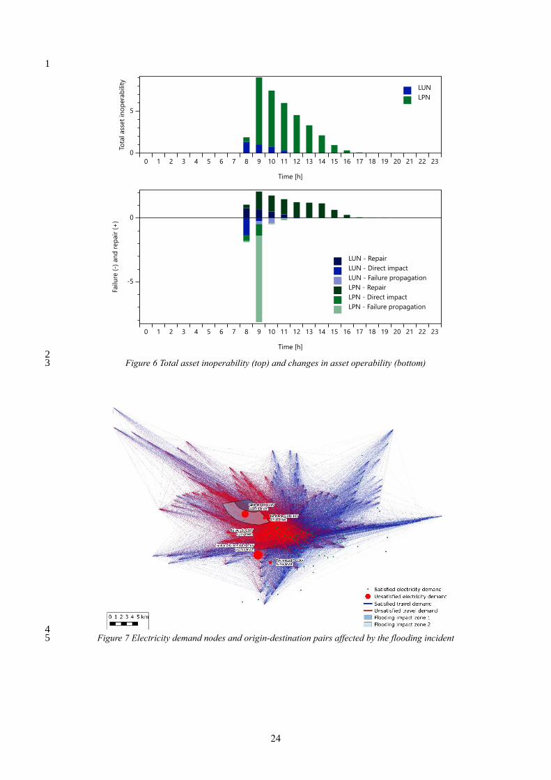
5.3.1. Asset failure and repair 14

Asset inoperability caused by direct and propagated failure after the flooding incident is shown in 15

Figure 6. In the first hour after the incident (𝑡 = 8), the expected number of asset failures over all 16

scenarios is 1.4 and 0.5 in the LUN and LPN respectively. In the second hour after the incident, the total 17

inoperability in the LUN system is expected to decrease to 1.1 due to the effective deployment of repair 18

resources which outweighs the additional damage caused by direct damage in flood zone 2 (0.2) and 19

failure propagation (0.2). In contrast, the total inoperability in the LPN system is predicted to rise 20

sharply to 8.0, mainly due to failure propagation (6.8) and also to direct damage in the second flood 21

zone (0.9). Due to the large number of asset failures, the LPN system is predicted to take 10 hours until 22

full recovery of asset operability whereas the LUN network is predicted to take only 5 hours. 23

24

1

2 Figure 6 Total asset inoperability (top) and changes in asset operability (bottom) 3

4 Figure 7 Electricity demand nodes and origin-destination pairs affected by the flooding incident 5

25

5.3.2. Unmet demand 1

The asset inoperability predicted by the model would severely affect the systems’ ability to meet the 2

demand of a typical weekday. Although the flood damage is contained to a relatively small area of the 3

city, its effects spread widely, as shown on the map of unmet demand in Figure 7. 4

The expected loss of electric power supply to two demand nodes located within the second flood 5

zone amounts to 172 MWh over the duration of the disruption. Additional 253 MWh of unmet demand 6

are expected to occur at three substations which are located south of the area affected by flooding. 7

The disruptions in the metro network mainly affect the Jubilee, Metropolitan and Bakerloo lines, 8

which run through the area affected by flooding and also depend on rolling stock, train control and 9

electric power supply assets located there. Hence, most journeys that are cancelled or delayed are to or 10

from areas served by these lines, most notably the Northwest of London. In total, the model predicts 11

that journeys between 7,321 OD pairs with a combined travel volume of 66,166 passenger journeys 12

would be affected by the disruption. 13

5.3.3. Value of demand and supply 14

The model predicts the expected loss (the difference between the value of demanded and supplied 15

infrastructure services) to amount to 1.3 and 7.2 million GBP in the transport and energy sectors 16

respectively. These results depend strongly on our assumptions regarding the value of infrastructure 17

services (A 2 and A 9). Figure 8 shows that although the estimated loss is in the range of millions, it is 18

still relatively small compared to the overall value of services provided by the infrastructure networks. 19

The simulation experiment enables us to quantify the resilience of the two interdependent 20

infrastructure systems in terms of the resilience measures introduced in Section 2. Figure 9 plots the 21

value-based system performance (1 −VoS𝑡

VoD𝑡) for the 74 individual scenarios and its probability-22

weighted average over all scenarios. The model predicts an average resilience loss triangle area (RLT) 23

of 0.11, an expected minimum system performance of 0.96 and a total length of disruption of 9 hours. 24

26

1

Figure 8 Value of demand (VoD) and expected value of supply (VoS) 2

3 Figure 9 Value-based system performance index 4

27

5.4. Sensitivity analysis 1

The simulation experiment was repeated with different parameter settings to analyse sensitivity. The 2

parameter for the capacity of engineering depots providing repair services was varied over the set 3

{0, 1, 2, 3}. Furthermore, three different levels for failure propagation probabilities were assumed. In 4

the first setting, the probability for short-range failure propagation (from the hazard to assets in flood 5

zone 1 or between assets less than 100 m apart) is 0.125 and the probability for long-range failure 6

propagation (from the hazard to assets in flood zone 2 or between assets 100 to 1,000 m apart) is 0.025. 7

In the second setting, the probabilities are 0.250 and 0.050 respectively, and in the third setting they are 8

0.500 and 0.100. The predicted RLT values for the resulting 12 parameter configurations are presented 9

in Figure 10. As expected, the sensitivity analysis shows that increasing the probability of failure 10

propagation increases the RLT area whereas increasing the capacity to provide repair services decreases 11

it. 12

13

Figure 10 RLT area for 12 parameter configurations denoted by [repair capacity, probability of 14 short-range failure propagation, probability of long-range failure propagation]. Dashed lines 15

indicate the probability-weighted mean. 16

The sensitivity analysis also demonstrates how the modelling framework presented in this paper 17

could be used to inform decision-making on how to improve the resilience of interdependent 18

infrastructure systems. For example, assume that the status quo is best represented by the parameter 19

setting [1, 0.250, 0.050] with an RLT area of 0.11. The model suggests that the resilience could be 20

improved to 0.06 at the cost of doubling the resources available for asset repair. Alternatively, the 21

resilience could be improved to 0.04 by investing in the protection of assets so that they are 50 % less 22

likely to suffer flood damage. A cost-benefit analysis based on such modelling and simulation results 23

28

could help decision-makers optimise strategies for strengthening infrastructure resilience and save 1

considerable financial resources compared to interventions not based on such evidence. 2

5.5. Discussion 3

The case study shows that the methodology presented in this paper can be used to create a complete 4

model of two real-world urban infrastructure networks relying only on publicly available data. Some 5

assumptions had to be made where data were not available, for example regarding hazard exposure and 6

repair resources. However, it is expected that future users of this modelling framework (e.g. 7

infrastructure companies) would be able to replace most of the assumptions with empirical data, thereby 8

improving the validity and accuracy of the analysis. 9

The case study illustrates that combining the network and asset representations of infrastructure 10

systems increases the level of detail at which infrastructure systems and their interdependencies can be 11

modelled. Aspects of infrastructure operations captured by this methodology that are outside the scope 12

of many existing models include the stochastic propagation of asset failure, hierarchical relations of 13

series or parallel sub-systems, and resource inputs from one system to another for the utilisation and 14

repair of assets. 15

Using a time-expanded graph and a rolling planning horizon, the method presented in this paper 16

models the optimal response to a disruption in terms of flow redistribution and repair resource 17

allocation. The model is based on the assumption that stochastic asset failure cannot be anticipated but 18

the effects of deploying repair resources can. However, the modelling framework would allow to modify 19

these assumptions. For example, one could include anticipation of asset failure based on (limited) 20

knowledge of failure propagation dependencies or a stochastic variation of repair effectiveness. 21

Even with the high level of operational detail captured by the proposed methodology, a dynamic, 22

city-scale model of two infrastructure systems with several thousands of assets, nodes, links and 23

dependency relations can be modelled and simulated with the computational resources of a standard 24

desktop computer. Compared to case studies presented for previous network flow models for 25

interdependent infrastructure networks, the system-of-systems analysed here is considerably larger and 26

the results offer more detailed insights into the phenomena determining infrastructure performance after 27

disruptive events. 28

While the minimum cost flow assignment model does not achieve the accuracy of more sophisticated 29

infrastructure-specific assignment models, it is suitable for resilience assessments seeking to cover a 30

large number of possible disruption scenarios. Its role in the modelling framework can be seen as a 31

placeholder model that can be replaced with more accurate assignment models if the required data inputs 32

for the latter are available and a smaller number of representative scenarios has been identified. 33

The optimisation problem formulated in this paper can be solved efficiently even for large problem 34

instances because it makes several approximations to avoid integer variables and non-linear equations. 35

29

For instance, the operability of a parallel system is assumed to be a linear combination and not the 1

maximum of the sub-systems’ operabilities. Resource inputs required by an asset are proportional to the 2

asset’s utilisation and do not include inputs that are required simply for the availability of an asset (e.g. 3

a metro station’s electric power base load). Such non-linear relationships could be modelled by 4

introducing binary decision variables but this would drastically increase the computational complexity. 5

6. CONCLUSION 6

By combining the network flow modelling paradigm with a novel representation of repairable 7

infrastructure assets, this paper makes some important contributions to improving resilience assessment 8

methods for interdependent infrastructure systems. An integrated and dynamic modelling framework is 9

presented that features a scenario tree generation algorithm for stochastic failure propagation and the 10

optimisation of network flows and repair resource allocation in response to a disruption. A rolling 11

planning horizon approach allows the model to make realistic assumptions regarding the anticipation 12

of asset failure and repair and enables the analysis of infrastructure resilience as opposed to static 13

network vulnerability. 14

The proposed modelling framework can be used by asset owners, network operators and 15

infrastructure planners to quantify the effects of changes regarding the configuration of infrastructure 16

systems and their exposure to hazards. Examples of interventions that could be evaluated include 17

investments in additional protection for infrastructure assets or resources for incident response. Users 18

of the model could either predict how the resilience performance measures would change after the 19

interventions or conduct experiments to estimate the investments required to achieve a certain level of 20

resilience against anticipated future hazard scenarios. The use of a value-based resilience measure 21

allows the direct use of model outputs in a cost-benefit analysis. 22

Further research could investigate in more detail how the linearity assumptions of the minimum cost 23

flow model affect the results and how the use of binary switching variables would affect its 24

computational complexity. Another direction of research could be to use the model presented here to 25

develop a criticality ranking method for infrastructure assets in a system-of-systems. Finally, it is 26

anticipated that future studies will extend the model to other types of infrastructure networks, for 27

example, road transport and communication networks. 28

7. ACKNOWLEDGEMENTS 29

The research was supported by the UK Engineering and Physical Sciences Research Council 30

(EPSRC) as part of the Sustainable Civil Engineering Centre for Doctoral Training (grant number 31

EP/L016826/1). 32

30

REFERENCES 1

[1] M. Kunz, B. Mühr, T. Kunz-Plapp, J. E. Daniell, B. Khazai, F. Wenzel, M. Vannieuwenhuyse, T. Comes, F. Elmer, K. 2 Schröter, J. Fohringer, T. Münzberg, C. Lucas, and J. Zschau, “Investigation of superstorm Sandy 2012 in a multi-3 disciplinary approach,” Nat. Hazards Earth Syst. Sci., vol. 13, no. 10, pp. 2579–2598, 2013. 4

[2] S. Kaufman, C. Qing, N. Levenson, and M. Hanson, “Transportation During and After Hurricane Sandy,” 2012. [Online]. 5 Available: http://wagner.nyu.edu/files/rudincenter/sandytransportation.pdf. [Accessed: 04-May-2018]. 6

[3] The City of New York, “A Stronger, More Resilient New York,” 2013. [Online]. Available: 7 http://www.nyc.gov/html/sirr/html/report/report.shtml. [Accessed: 11-May-2017]. 8

[4] S. E. Chang, T. L. McDaniels, J. Mikawoz, and K. Peterson, “Infrastructure failure interdependencies in extreme events: 9 power outage consequences in the 1998 Ice Storm,” Nat. Hazards, vol. 41, pp. 337–358, Nov. 2007. 10

[5] M. Rong, C. Han, and L. Liu, “Critical Infrastructure Failure Interdependencies in the 2008 Chinese Winter Storms,” in 11 2010 International Conference on Management and Service Science (MASS), 2010. 12

[6] L. Dueñas-Osorio and A. Kwasinski, “Quantification of Lifeline System Interdependencies after the 27 February 2010 13 Mw 8.8 Offshore Maule, Chile, Earthquake,” Earthq. Spectra, vol. 28, no. S1, pp. S581–S603, Jun. 2012. 14

[7] T. D. O’Rourke, S.-S. Jeon, S. Toprak, M. Cubrinovski, M. Hughes, S. van Ballegooy, and D. Bouziou, “Earthquake 15 Response of Underground Pipeline Networks in Christchurch, NZ,” Earthq. Spectra, vol. 30, no. 1, pp. 183–204, Feb. 16 2014. 17

[8] BBC, “Holborn underground fire: Electrical fault caused 36-hour blaze,” 2015. [Online]. Available: 18 http://www.bbc.co.uk/news/uk-england-london-32231725. [Accessed: 04-May-2018]. 19

[9] S. M. Rinaldi, J. P. Peerenboom, and T. K. Kelly, “Identifying, Understanding, and Analyzing Critical Infrastructure 20 Interdependencies,” IEEE Control Syst. Mag., vol. 21, no. 6, pp. 11–25, Dec. 2001. 21

[10] S. Hosseini, K. Barker, and J. E. Ramirez-Marquez, “A review of definitions and measures of system resilience,” Reliab. 22 Eng. Syst. Saf., vol. 145, pp. 47–61, 2016. 23

[11] R. Zimmerman, “Social Implications of Infrastructure Network Interactions,” J. Urban Technol., vol. 8, no. 3, pp. 97–24 119, Dec. 2001. 25

[12] D. D. Dudenhoeffer, M. R. Permann, and C. Miller, “Interdependency Modeling and Emergency Response,” in 26 Proceedings of the 2007 Summer Computer Simulation Conference, 2007, pp. 1230–1237. 27

[13] A. Volkanovski, M. Čepin, and B. Mavko, “Application of the fault tree analysis for assessment of power system 28 reliability,” Reliab. Eng. Syst. Saf., vol. 94, no. 6, pp. 1116–1127, 2009. 29

[14] H.-S. J. Min, W. Beyeler, T. Brown, Y. J. Son, and A. T. Jones, “Toward modeling and simulation of critical national 30 infrastructure interdependencies,” IIE Trans., vol. 39, no. 1, pp. 57–71, Jan. 2007. 31

[15] C. Nan and G. Sansavini, “A quantitative method for assessing resilience of interdependent infrastructures,” Reliab. Eng. 32 Syst. Saf., vol. 157, pp. 35–53, 2017. 33

[16] Y. Y. Haimes and P. Jiang, “Leontief-Based Model of Risk in Complex Interconnected Infrastructures,” J. Infrastruct. 34 Syst., vol. 7, no. 1, pp. 1–12, 2001. 35

[17] L. Dueñas-Osorio, J. Craig, and B. Goodno, “Seismic response of critical interdependent networks,” Earthq. Eng. Struct. 36 Dyn., vol. 36, pp. 285–306, 2007. 37

[18] E. E. Lee II, J. E. Mitchell, and W. A. Wallace, “Restoration of Services in Interdependent Infrastructure Systems: A 38 Network Flows Approach,” IEEE Trans. Syst. Man, Cybern. Part C Appl. Rev., vol. 37, no. 6, pp. 1303–1317, Nov. 2007. 39

[19] S. Buldyrev, R. Parshani, G. Paul, H. E. Stanley, and S. Havlin, “Catastrophic cascade of failures in interdependent 40 networks,” Nature, vol. 464, pp. 1025–8, 2010. 41

[20] R. Holden, D. V. Val, R. Burkhard, and S. Nodwell, “A network flow model for interdependent infrastructures at the 42 local scale,” Saf. Sci., vol. 53, pp. 51–60, 2013. 43

[21] R. M. D’Souza, C. D. Brummitt, and E. A. Leicht, “Modeling Interdependent Networks as Random Graphs: Connectivity 44 and Systemic Risk,” in Networks of Networks: The Last Frontier of Complexity, G. D’Agostino and A. Scala, Eds. Cham: 45 Springer, 2014. 46

[22] J. G. Jin, L. C. Tang, L. Sun, and D. H. Lee, “Enhancing metro network resilience via localized integration with bus 47 services,” Transp. Res. Part E Logist. Transp. Rev., vol. 63, pp. 17–30, 2014. 48

[23] H. Fotouhi, S. Moryadee, and E. Miller-Hooks, “Quantifying the Resilience of an Urban Traffic-Electric Power Coupled 49 System,” Reliab. Eng. Syst. Saf., vol. 163, pp. 79–94, 2017. 50

[24] S. Thacker, R. Pant, and J. W. Hall, “System-of-systems formulation and disruption analysis for multi-scale critical 51 national infrastructures,” Reliab. Eng. Syst. Saf., vol. 167, no. January 2015, pp. 30–41, 2017. 52

[25] M. Ouyang, “Review on modeling and simulation of interdependent critical infrastructure systems,” Reliab. Eng. Syst. 53 Saf., vol. 121, pp. 43–60, 2014. 54

[26] M. Iturriza, L. Labaka, J. M. Sarriegi, and J. Hernantes, “Modelling methodologies for analysing critical infrastructures,” 55

31

J. Simul., vol. 12, no. 2, pp. 128–143, 2018. 1

[27] E. Zio, “Challenges in the vulnerability and risk analysis of critical infrastructures,” Reliab. Eng. Syst. Saf., vol. 152, pp. 2 137–150, 2016. 3

[28] P. Hines, E. Cotilla-Sanchez, and S. Blumsack, “Do topological models provide good information about electricity 4 infrastructure vulnerability?,” Chaos, vol. 20, no. 3, Sep. 2010. 5

[29] M. Ouyang, “Comparisons of purely topological model, betweenness based model and direct current power flow model 6 to analyze power grid vulnerability.,” Chaos, vol. 23, no. 2, Jun. 2013. 7

[30] M. Ouyang, L. Zhao, L. Hong, and Z. Pan, “Comparisons of complex network based models and real train flow model 8 to analyze Chinese railway vulnerability,” Reliab. Eng. Syst. Saf., vol. 123, pp. 38–46, Mar. 2014. 9

[31] M. Ouyang, “Critical location identification and vulnerability analysis of interdependent infrastructure systems under 10 spatially localized attacks,” Reliab. Eng. Syst. Saf., vol. 154, pp. 106–116, 2016. 11

[32] A. Azzolin, L. Dueñas-Osorio, F. Cadini, and E. Zio, “Electrical and topological drivers of the cascading failure dynamics 12 in power transmission networks,” Reliab. Eng. Syst. Saf., vol. 175, no. March, pp. 196–206, 2018. 13

[33] W. Sun, P. Bocchini, and B. D. Davison, “Resilience metrics and measurement methods for transportation infrastructure : 14 the state of the art,” Sustain. Resilient Infrastruct., vol. 9689, pp. 1–33, 2018. 15

[34] M. Bruneau, S. E. Chang, R. T. Eguchi, G. C. Lee, T. D. O’Rourke, A. M. Reinhorn, M. Shinozuka, K. Tierney, W. a. 16 Wallace, and D. von Winterfeldt, “A Framework to Quantitatively Assess and Enhance the Seismic Resilience of 17 Communities,” Earthq. Spectra, vol. 19, no. 4, pp. 733–752, Nov. 2003. 18

[35] M. Ouyang, L. Dueñas-Osorio, and X. Min, “A three-stage resilience analysis framework for urban infrastructure 19 systems,” Struct. Saf., vol. 36–37, no. 0, pp. 23–31, 2012. 20

[36] P. Angeloudis and D. Fisk, “Large subway systems as complex networks,” Phys. A Stat. Mech. its Appl., vol. 367, pp. 21 553–558, 2006. 22

[37] A. M. Caunhye, Y. Zhang, M. Li, and X. Nie, “A location-routing model for prepositioning and distributing emergency 23 supplies,” Transp. Res. Part E Logist. Transp. Rev., vol. 90, pp. 161–176, 2016. 24

[38] W. Zhang, N. Wang, and C. Nicholson, “Resilience-based post-disaster recovery strategies for road-bridge networks,” 25 Struct. Infrastruct. Eng., vol. 13, no. 11, pp. 1404–1413, 2017. 26

[39] L. Faramondi, R. Setola, S. Panzieri, F. Pascucci, and G. Oliva, “Finding critical nodes in infrastructure networks,” Int. 27 J. Crit. Infrastruct. Prot., vol. 20, pp. 3–15, 2018. 28

[40] C. D. Nicholson, K. Barker, and J. E. Ramirez-Marquez, “Flow-based vulnerability measures for network component 29 importance: Experimentation with preparedness planning,” Reliab. Eng. Syst. Saf., vol. 145, pp. 62–73, Jan. 2016. 30

[41] D. L. Alderson, G. G. Brown, and W. M. Carlyle, “Assessing and Improving Operational Resilience of Critical 31 Infrastructures and Other Systems,” in INFORMS 2014 Tutorials in Operations Research, 2014, no. November. 32

[42] P. Trucco, E. Cagno, and M. De Ambroggi, “Dynamic functional modelling of vulnerability and interoperability of 33 Critical Infrastructures,” Reliab. Eng. Syst. Saf., vol. 105, pp. 51–63, Sep. 2012. 34

[43] L. Chen and E. Miller-Hooks, “Resilience: An Indicator of Recovery Capability in Intermodal Freight Transport,” Transp. 35 Sci., vol. 46, no. 1, pp. 109–123, 2012. 36

[44] P. Chopade and M. Bikdash, “New centrality measures for assessing smart grid vulnerabilities and predicting brownouts 37 and blackouts,” Int. J. Crit. Infrastruct. Prot., vol. 12, pp. 29–45, 2014. 38

[45] R. Faturechi and E. Miller-Hooks, “Travel time resilience of roadway networks under disaster,” Transp. Res. Part B 39 Methodol., vol. 70, pp. 47–64, 2014. 40

[46] M. Nogal, A. O’Connor, B. Caulfield, and B. Martinez-Pastor, “Resilience of Traffic Networks: From Perturbation to 41 Recovery via a Dynamic Restricted Equilibrium Model,” Reliab. Eng. Syst. Saf., vol. 156, pp. 84–96, 2016. 42

[47] O. Cats, G. J. Koppenol, and M. Warnier, “Robustness assessment of link capacity reduction for complex networks: 43 Application for public transport systems,” Reliab. Eng. Syst. Saf., vol. 167, no. July, pp. 544–553, 2017. 44

[48] J. C. Lam, M. Heitzler, J. Hackl, and B. T. Adey, “Modelling the functional capacity losses of networks exposed to 45 hazards,” Sustain. Resilient Infrastruct., vol. 9689, no. May, pp. 1–19, 2018. 46

[49] O. Cats and E. Jenelius, “Planning for the unexpected: The value of reserve capacity for public transport network 47 robustness,” Transp. Res. Part A Policy Pract., vol. 81, pp. 47–61, 2015. 48

[50] M. K. Miller and J. W. Baker, “Coupling mode-destination accessibility with seismic risk assessment to identify at-risk 49 communities,” Reliab. Eng. Syst. Saf., vol. 147, pp. 60–71, 2015. 50

[51] G. P. Cimellaro, A. M. Reinhorn, and M. Bruneau, “Framework for analytical quantification of disaster resilience,” Eng. 51 Struct., vol. 32, no. 11, pp. 3639–3649, 2010. 52

[52] M. Fonoberova, “Optimal Flows in Dynamic Networks and Algorithms for their Finding,” in Handbook of Optimization 53 in Complex Networks: Theory and Applications, M. T. Thai and P. M. Pardalos, Eds. Boston, MA: Springer US, 2012, 54 pp. 363–403. 55

[53] R. K. Ahuja, T. L. Magnanti, and J. B. Orlin, Network Flows: Theory, Algorithms, and Applications. Prentice Hall, 1993. 56

32

[54] J. Y. Yen, “Finding the K Shortest Loopless Paths in a Network,” Manage. Sci., vol. 17, no. 11, pp. 712–716, 1971. 1

[55] UK Power Networks PLC, “Long Term Development Statement,” 2017. [Online]. Available: 2 https://www.ukpowernetworks.co.uk/internet/en/about-us/regulatory-information/long-term-development-3 statement.html. 4

[56] Transport for London, “Rolling Origin and Destination Survey,” 2016. [Online]. Available: https://tfl.gov.uk/info-5 for/open-data-users/. [Accessed: 04-May-2018]. 6

[57] London Borough of Brent, “Strategic Flood Risk Assessment (SFRA) Level 1,” 2007. [Online]. Available: 7 http://geosmartinfo.co.uk/wp-content/uploads/sfra/Strategic-flood-report-2007.pdf. [Accessed: 04-May-2018]. 8

[58] London Borough of Brent, “Flood Risk Management Strategy: Managing the Floods Risk in Brent,” 2015. [Online]. 9 Available: https://www.brent.gov.uk/media/16406897/flood-risk-strategy-sept-2015.pdf. [Accessed: 04-May-2018]. 10

[59] “London Underground Track and Traction Current,” 2000. [Online]. Available: 11 http://www.trainweb.org/tubeprune/tractioncurr.htm. [Accessed: 04-May-2018]. 12

[60] London Economics, “The Value of Lost Load (VoLL) for Electricity in Great Britain: Final report for OFGEM and 13 DECC,” 2013. [Online]. Available: https://www.ofgem.gov.uk/ofgem-publications/82293/london-economics-value-lost-14 load-electricity-gbpdf. [Accessed: 04-May-2018]. 15

[61] Transport for London, “Unified API.” [Online]. Available: https://api.tfl.gov.uk/. [Accessed: 04-May-2018]. 16

[62] Transport for London, “FOI-0175-1314: Station to Station Journey Times,” 2013. [Online]. Available: 17 https://www.whatdotheyknow.com/request/station_to_station_journey_times. [Accessed: 04-May-2018]. 18

[63] Transport for London, “FOI-1216-1112: Gate-to-platform and interchange walking times,” 2012. [Online]. Available: 19 https://www.whatdotheyknow.com/request/gate_to_platform_and_interchange. [Accessed: 04-May-2018]. 20

[64] UK Department for Transport, “Provision of market research for value of travel time savings and reliability,” 2015. 21 [Online]. Available: https://www.gov.uk/government/publications/values-of-travel-time-savings-and-reliability-final-22 reports. [Accessed: 04-May-2018]. 23

[65] Carto Metro, “Detailed map of London Tube, Underground, Overground, DLR, Tramlink & National Rail,” 2017. 24 [Online]. Available: http://carto.metro.free.fr/metro-london/. [Accessed: 04-May-2018]. 25

[66] Transport for London, “TfL Energy Purchasing 2020 to 2023,” 2017. [Online]. Available: http://content.tfl.gov.uk/fc-26 20171205-part-1-item08-tfl-energy-purchasing-2020-2023.pdf. [Accessed: 04-May-2018]. 27

28

33

APPENDIX 1

2

Table 4 Infrastructure systems, components and parameters 3

System Component Para-meter

Value / description Data sources Assump-tions

LPN Nodes 𝑉SC 1,379 nodes including: 1,294 busbars (voltage levels 11 to 132 kV), 6 bulk supply points for traction power, 79 traction power supply substations

UKPN LTDS [55]

Trainweb [59]

𝑔𝑖𝑡 Rated capacity of 67 super-grid transformers UKPN LTDS [55]

Links 𝐸SC 1,742 links including: 828 connectors, 394 two-winding transformers, 80 three-winding transformers, reverse direction links where applicable

UKPN LTDS [55]

𝑓𝑖,𝑗𝑡 Cables and transformers: rated capacity

Intra-substation connectors: unlimited

UKPN LTDS [55]

Assets 𝐴 392 assets including: 19 grid supply points, 247 high-voltage substations, 126 low-voltage substations

UKPN LTDS [55]

Demand �̌�𝑖𝑡 Load profiles for 128 demand nodes derived from peak demand

and minimum load scaling factor UKPN LTDS [55] A 1

𝑣𝑖SC 16,940 GBP/MWh (weighted average value of lost load for peak

winter workdays in the UK) London Econ. [60] A 2

LPN repair

Nodes 𝑉SC 12 engineering depots, 392 potential repair sites UKPN LTDS [55]

𝑔𝑖𝑡 Engineering depots: 1 repair resource units per hour A 3

Links 𝐸SC 784 repair resource deployment links A 4

𝑓𝑖,𝑗𝑡 0.25 if distance is less than 10 km

0.20 if distance is between 10 and 25 km 0.17 if distance is greater than 25 km

A 5

LUN Nodes 𝑉MC 1,045 nodes including: 267 stations, 778 platforms TfL RODS [56]

Links 𝐸MC 2,315 links including: 759 on-train links, 778 boarding links, 778 alighting links

TfL RODS [56]

𝑓𝑖,𝑗𝑡 On-train-links: Number of scheduled train departures per hour

multiplied with rolling stock capacity

Boarding and alighting links: capacity estimated based on maximum station entries and exits

TfL API [61] A 6

𝑐𝑖,𝑗f On-train-links: station-to-station journey times

Alighting links: platform-to-ticket-hall walking time

Boarding links: ticket-hall-to-platform walking time plus average waiting time for first train

All travel times valued at 11.21 GBP/h

TfL FOIs [62], [63]

TfL API [61]

DfT VoTT [64]

A 7

Assets 𝐴 389 assets including: 267 stations, 79 track sections, 8 line control systems, 8 rolling stock fleets, 8 control centres, 19 depots

TfL RODS [56]

Trainweb [59]

Carto Metro [65]

Demand 𝑓𝑜,𝑑𝑡 Travel demand profiles for 32,109 OD pairs TfL RODS [56] A 8

𝑣𝑜,𝑑MC Cost of alternative transport modes estimated based on

geographic distance A 9

LUN repair

Nodes 𝑉SC 19 engineering depots, 373 potential repair sites Carto Metro [65]

𝑔𝑖𝑡 Engineering depots: 1 repair resource units per hour A 3

Links 𝐸SC 957 repair resource deployment links A 4

𝑓𝑖,𝑗𝑡 0.25 if distance is less than 10 km

0.20 if distance is between 10 and 25 km 0.17 if distance is greater than 25 km

A 5

34

Table 5 Dependency relations 1

Dependency type

From To No. of instances

Parameters Assump-tions

Failure propagation

Flood hazard Assets in flood zone 1 9 𝑝ℎ,𝑘 = 0.250

𝑡ℎ,𝑘 = 0

A 10

Flood hazard Assets in flood zone 2 30 𝑝ℎ,𝑘 = 0.050

𝑡ℎ,𝑘 = 1

A 10

Asset 𝑘 ∈ 𝐴 Assets located less than 100 m from 𝑘

1,598 𝑝ℎ,𝑘 = 0.250

𝑡ℎ,𝑘 = 0

A 11

Asset 𝑘 ∈ 𝐴 Assets located between 100 and

1,000 m from 𝑘

5,940 𝑝ℎ,𝑘 = 0.050

𝑡ℎ,𝑘 = 1

A 11

Asset utilisation

Electricity substation assets 𝑘 Supply nodes located at 𝑘 and

links starting or ending at 𝑘

4,837

Metro station asset 𝑘 Boarding and alighting links of 𝑘 1,556

Track section asset 𝑘 On-train links that use 𝑘 759

Logic Line control assets Track section assets 79

Rolling stock fleet assets Track section assets 79

Control centre assets Line control assets 10

Depot assets Rolling stock fleet assets 20

Input Low-voltage electricity substation node

Metro station asset 534 𝛼𝑖,𝑘U = 0.10 A 12

Traction power supply substation node

Track section assets 79 𝛼𝑖,𝑘U = 4.00 A 13

Potential repair site node Asset 765 𝛼𝑖,𝑘R = 1.00 A 14

2

35

Table 6 Overview of modelling assumptions 1

No. System Assumption Justification

A 1 LPN Time series of substation loads can be estimated by fitting a generic load profile to the peak and minimum load available from the UKPN LTDS [55].

Standard method used in the absence of time series load data

A 2 LPN The weighted average value of lost load specified in London Economics [60] as 16,940 GBP/MWh applies to all demand nodes.

Best available estimate for economic cost of power outages

A 3 LPN repair & LUN repair

Each engineering depot can dispatch 1 units of repair resources per time step.

Sensitivity analysis provided


Depots can be repaired by local engineering teams, control centre assets can be repaired by engineering teams from any depot, track sections can be repaired by the depot belonging to the respective line, metro stations and electricity substations can be repaired by the two nearest depots.

Estimate based on subject matter expertise


The time to repair an asset is determined by the distance from the engineering depot carrying out the repair (4 hours if less than 10 km, 5 hours if between 10 and 25 km, 6 hours if greater than 25 km).

Estimate based on subject matter expertise

A 6 LUN Boarding and alighting links have an excess capacity of 10 % with respect to the maximum station entries or exits recorded in [56] but not less than 5,000 passengers per hour.

Most metro stations in central London are near capacity during peak hours

A 7 LUN All passengers value travel time at 11.21 GBP/h. Assumption necessary due to the unavailability of trip purpose data

A 8

LUN Time series of travel demands can be estimated by distributing travel demand given in TfL RODS [56] for 6 daily time slots uniformly within the respective time slot and calculating the moving average over three hours.

Standard smoothing method for demand forecasting

A 9 LUN The value of the transportation services provided can be estimated as:

5 GBP +Distance in km

5kmh

× 11.21GBP

h

The relatively high value is justified because in the case of major disruptions the cost of alternative transport modes is likely to be above average, e.g. due to congestion

A 10 LPN & LUN Assets located less than 2,000 m from the reservoir suffer flood damage with

a probability of 33 % and no time lag. Assets located at a distance between

2,000 and 4,000 m are damaged with a probability of 10 % and a time lag of

1 hour.

Hypothetical flood risk exposure

A 11 LPN & LUN Failure propagates between assets located less than 100 m apart with a

probability of 33 % and no time lag, and between assets located between 100

and 1,000 m apart with a probability of 5 % and a time lag of 1 hour.

Hypothetical failure propagation risk exposure

A 12 LPN & LUN Metro stations require a power supply of 0.1 MW when used at full capacity. Estimate based on dividing London Undergrounds total non-traction power consumption of 200 GWh/a [66] by the number of stations and assuming a peak-to-average ratio of 1.2

A 13 LPN & LUN Track sections require a power supply of 4.0 MW when being used at full

capacity.

Estimate based on dividing London Undergrounds total traction power consumption of 1,363 GWh/a [66] by the number of track sections and assuming a peak-to-average ratio of 2.0

A 14 LPN & LUN Failed asset requires 1 unit of repair resources to be fully repaired. Based on the assumption that all flood damage incidents are of similar magnitude

2

Resilience assessment for interdependent urban ... · Section 4 presents the integrated asset...

Documents

Transcript of Resilience assessment for interdependent urban ... · Section 4 presents the integrated asset...