Residential Mechanical Precoolingapps1.eere.energy.gov/buildings/publications/pdfs/... ·...

Residential Mechanical Precooling Alea German and Marc Hoeschele Alliance for Residential Building Innovation

December 2014

NOTICE

This report was prepared as an account of work sponsored by an agency of the United States government. Neither the United States government nor any agency thereof, nor any of their employees, subcontractors, or affiliated partners makes any warranty, express or implied, or assumes any legal liability or responsibility for the accuracy, completeness, or usefulness of any information, apparatus, product, or process disclosed, or represents that its use would not infringe privately owned rights. Reference herein to any specific commercial product, process, or service by trade name, trademark, manufacturer, or otherwise does not necessarily constitute or imply its endorsement, recommendation, or favoring by the United States government or any agency thereof. The views and opinions of authors expressed herein do not necessarily state or reflect those of the United States government or any agency thereof.

Available electronically at http://www.osti.gov/bridge

Available for a processing fee to U.S. Department of Energy and its contractors, in paper, from:

U.S. Department of Energy Office of Scientific and Technical Information P.O. Box 62 Oak Ridge, TN 37831-0062 phone: 865.576.8401 fax: 865.576.5728 email: mailto:[email protected]

Available for sale to the public, in paper, from:

U.S. Department of Commerce National Technical Information Service 5285 Port Royal Road Springfield, VA 22161 phone: 800.553.6847 fax: 703.605.6900 email: [email protected] online ordering: http://www.ntis.gov/ordering.htm

http://www.osti.gov/bridge

mailto:[email protected]

mailto:[email protected]

http://www.ntis.gov/ordering.htm

iii

Residential Mechanical Precooling

Prepared for:

The National Renewable Energy Laboratory

On behalf of the U.S. Department of Energy’s Building America Program

Office of Energy Efficiency and Renewable Energy

15013 Denver West Parkway

Golden, CO 80401

NREL Contract No. DE-AC36-08GO28308

Prepared by:

Alea German and Marc Hoeschele

Alliance for Residential Building Innovation

Davis Energy Group, Team Lead

123 C Street

Davis, CA 95616

NREL Technical Monitor: Stacey Rothgeb

Prepared under Subcontract No. KNDJ-0-40340-04

December 2014

iv

The work presented in this report does not represent performance of any product relative to regulated minimum efficiency requirements. The laboratory and/or field sites used for this work are not certified rating test facilities. The conditions and methods under which products were characterized for this work differ from standard rating conditions, as described. Because the methods and conditions differ, the reported results are not comparable to rated product performance and should only be used to estimate performance under the measured conditions.

v

Contents List of Figures ............................................................................................................................................ vi List of Tables .............................................................................................................................................. vi Definitions .................................................................................................................................................. vii Executive Summary ................................................................................................................................. viii 1 Introduction and Background ............................................................................................................. 1

1.1 Objectives ........................................................................................................................................ 1 1.2 Previous Research ............................................................................................................................ 2 1.3 Considerations ................................................................................................................................. 2

2 Methodology ......................................................................................................................................... 5 2.1 House Monitoring ............................................................................................................................ 5 2.2 EnergyPlus Modeling....................................................................................................................... 5 2.3 Presentation of Results ..................................................................................................................... 9

3 Results ................................................................................................................................................. 13 4 Conclusions and Discussion ............................................................................................................ 16 References ................................................................................................................................................. 18 Appendix: Modeling Results From EnergyPlus Simulations ............................................................... 19

vi

List of Figures Figure 1. Example results figure with description for interpretation .................................................. 10 Figure 2. Description of results figures—top two graphs .................................................................... 10 Figure 3. Description of results figures—middle two graphs .............................................................. 11 Figure 4. Description of results figures—bottom graph ....................................................................... 12 Figure 5. Recommended operating strategies and associated energy and utility cost impacts

for a 2,150-ft2 Benchmark home in CZ 1A (Miami) .......................................................................... 20 Figure 6. Recommended operating strategies and associated energy and utility cost impacts

for a 2,150-ft2 high performance home in CZ 1A (Miami) ............................................................... 21 Figure 7. Recommended operating strategies and associated energy and utility cost impacts

for a 2,150-ft2 Benchmark home in CZ 2A (Houston) ...................................................................... 22 Figure 8. Recommended operating strategies and associated energy and utility cost impacts

for a 2,150-ft2 high performance home in CZ 2A (Houston) ........................................................... 23 Figure 9. Recommended operating strategies and associated energy and utility cost impacts

for a 2,150-ft2 Benchmark home in CZ 2B (Phoenix) ...................................................................... 24 Figure 10. Recommended operating strategies and associated energy and utility cost impacts

for a 2,150-ft2 high performance home in CZ 2B (Phoenix) ............................................................ 25 Figure 11. Recommended operating strategies and associated energy and utility cost impacts

for a 2,150-ft2 Benchmark home in CZ 3B (Las Vegas) ................................................................... 26 Figure 12. Recommended operating strategies and associated energy and utility cost impacts

for a 2,150-ft2 high performance home in CZ 3B (Las Vegas) ........................................................ 27 Figure 13. Recommended operating strategies and associated energy and utility cost impacts

for a 2,150-ft2 Benchmark home in CZ 4A (Kansas City) ................................................................ 28 Figure 14. Recommended operating strategies and associated energy and utility cost impacts

for a 2,150-ft2 high performance home in CZ 4A (Kansas City) ..................................................... 29 Figure 15. Recommended operating strategies and associated energy and utility cost impacts

for a 2,150-ft2 Benchmark home in CZ 5A (Boston) ........................................................................ 30 Figure 16. Recommended operating strategies and associated energy and utility cost impacts

for a 2,150-ft2 high performance home in CZ 5A (Boston) ............................................................. 31 Figure 17. Recommended operating strategies and associated energy and utility cost impacts

for a 2,150-ft2 Benchmark home in CZ 5B (Denver) ........................................................................ 32 Figure 18. Recommended operating strategies and associated energy and utility cost impacts

for a 2,150-ft2 high performance home in CZ 5B (Denver) ............................................................. 33

Unless otherwise noted, all figures were created by the Alliance for Residential Building Innovation team.

List of Tables Table 1. Building Characteristics Applied in the Energy Model............................................................. 6 Table 2. Set Point Control Strategies Evaluated in the Energy Model .................................................. 7 Table 3. Cooling System Sizing and Simulation Details ......................................................................... 8 Table 4. Maximum Energy Savings Results for Benchmark Case for the Hottest Days ................... 14 Table 5. Minimize Coincident Peak Demand Results for Benchmark Case for the Hottest Days .... 14 Table 6. Maximum Energy Savings Results for High Performance Case for the Hottest Days ........ 15 Table 7. Minimum Coincident Peak Demand Results for High Performance Case for the Hottest

Days ..................................................................................................................................................... 15

Unless otherwise noted, all tables were created by the Alliance for Residential Building Innovation team.

vii

Definitions

AC Air Conditioner, Air Conditioning

BEopt™ Building Energy Optimization software

CZ Climate Zone

IECC International Energy Conservation Code

SHGC Solar Heat Gain Coefficient

TOU Time of Use

viii

Executive Summary

Residential air conditioning (AC) represents a challenging load for many electric utilities with poor load factors. Mechanical precooling improves the load factor by shifting cooling operation from on-peak to off-peak hours. This provides benefits to utilities and the electricity grid, as well as to occupants who can take advantage of time-of-use (TOU) electricity rates. Performance benefits stem from reduced compressor cycling, and shifting condensing unit operation to earlier periods of the day when outdoor temperatures are more favorable to operational efficiency. Finding solutions that save energy and reduce demand on the electricity grid is an important national objective and supports key Building America goals.

The Alliance for Residential Building Innovation team evaluated mechanical AC precooling strategies in homes throughout the United States. EnergyPlus modeling was used to evaluate two homes with different performance characteristics in seven climates. Results are applicable to new construction homes and most existing homes built in the last 10 years, as well as fairly efficient retrofitted homes. A successful off-peak AC strategy offers the potential for increased efficiency and improved occupant comfort, and promotes a more reliable and robust electricity grid. Demand response capabilities and further integration with photovoltaic TOU generation patterns provide additional opportunities to flatten loads and optimize grid impacts. Some key lessons learned from the results follow:

• Energy savings are difficult to achieve with precooling alone. In most cases, particularly on hotter summer days, no precooling strategy (without a subsequent thermostat setup during the peak hours) resulted in cooling energy savings. In instances where energy savings were achieved, they were very minimal (≤ 2%). Although not a precooling strategy by itself, a thermostat setup of 2°F during the peak hours resulted in estimated annual cooling energy savings of 2%–10%.

• Projected coincident peak demand reductions were greater in the high performance home. A home with greater envelope integrity provides better storage capability, increasing the effectiveness of precooling.

• Precooling combined with a 2°F thermostat setup during peak hours eliminated AC coincident peak demand in the high performance home in all scenarios, except on days when the average outdoor temperature exceeded 80°F in Phoenix (climate zone 2B). Alternatively, results with the 78°F peak setup demonstrated 100% demand savings for the Benchmark in only two climates.

• A strategy focused on minimizing coincident peak demand was found to have a nontrivial impact on energy consumption. In the high performance home energy use increased by 2%–8%, or up to 105 kWh, with precooling that targeted demand savings. This conclusion may be interpreted differently depending upon the stakeholder’s viewpoint.

• Cost savings are very dependent on the utility rates and the on-peak time period. The utility costs presented in the report are based on a generic TOU tariff. Actual costs and savings will be highly dependent on the rate structures available to customers. Future advances in real-time pricing should result in more favorable precooling economics because higher peak period pricing tariffs are more representative of reality.

ix

SmartGrid-driven innovations and communicating thermostats allow additional refinement and sophistication to be added to precooling. Smart controls can learn how the building responds and what comfort conditions occupants desire by time of day, and can use next-day forecasted outdoor temperatures to determine optimal precooling targets. Several advanced thermostat manufacturers and cloud-based systems implementing such strategies have been demonstrated with major utilities in the southwestern United States in the past few years. With increased interest from utilities and greater sophistication in controls and appliance connectivity, the authors foresee that residential precooling will become more tailored to a specific house, the day’s predicted weather, occupant patterns, and a utility’s predicted demands.

1

1 Introduction and Background

Air conditioners (ACs) are present in nearly all newly built production homes throughout the United States, and some form of mechanical AC equipment is found in 87% of all U.S. homes, based on the U.S. Department of Energy’s 2009 Residential Energy Consumption Survey (EIA 2009). According to these data, cooling represents about 6% of annual residential site energy consumption nationally,1 but its impact on utility peak demand is much more significant. This is especially true in hot-dry climates in the western United States, where residential cooling loads are more concentrated around the hottest hours of the day. For example, California residential AC represents about 15% of the state’s peak coincident electricity demand, but only 2% of annual electricity consumption (Brown and Koomey 2002).2

Growing peak demand forces utilities to rely increasingly on lower efficiency “peaker” plants that are activated to support the incremental electricity load during peak hours. Finding solutions that save energy and reduce electricity demands on the electricity grid is an important national objective and supports key Building America goals.

Precooling is an operational strategy—with potentially no upfront costs—that cools occupied spaces earlier in the day to avoid afternoon AC operation. In its simplest form, precooling can be implemented by scheduling AC operation to reduce set points 2°–6°F below typical settings in advance of the utility on-peak period. Performance benefits stem from reduced compressor cycling degradation and shifting condensing unit operation to earlier periods of the day when outdoor temperatures are more favorable to operational efficiency. Precooling can also use cool nighttime outdoor air for cooling, allowing more efficient fan-forced ventilation to offset compressor operation. The benefits of precooling can be counteracted by an unavoidable lack of precision in the application of precooling, particularly in homes with insufficient thermal mass, which may result in overcooling on milder days, and greater conduction losses caused by lower indoor temperatures.

1.1 Objectives The primary focus of this research is to identify best practice strategies for AC precooling in residential homes in various climates throughout the United States. The evaluation approach applied a combination of EnergyPlus simulation modeling and field monitoring to quantify energy and demand savings. Key factors explored in this study include the impacts of:

• House “efficiency” characteristics (thermal mass; envelope and heating, ventilation, and air conditioning thermal performance; and infiltration rates)

• Climate impacts

• Utility rates.

Although the application of precooling is more straightforward in hot-dry climates, this research also looked at impacts in humid climates. Applying precooling may create more variation in 1 0.635 quads out of a total 10.183 quads of residential consumption annually. 2 Commercial building air conditioning in California represents about 5% of statewide consumption, but a slightly lower 14% of coincident peak demand. The resulting load factor for commercial cooling is therefore nearly three times higher than for the residential sector.

2

interior relative humidity in humid climates; however, humidity control can be accomplished with standalone dehumidifiers, as documented in prior Building America research (Rudd 2014; Rudd et al. 2005). This study focuses on newly built homes, existing homes built in the last 10 years, and energy-efficient retrofitted homes. Minimal benefits from precooling were found in older homes; therefore, these findings are not presented in this study.

1.2 Previous Research Although considerable work has been completed in commercial building precooling over the past several decades (Xu et al. 2004; Smith and Braun 2003), research efforts in the residential space are much more limited. This may be due to the assumption that larger commercial buildings represent a bigger opportunity for engagement, as opposed to the more diffuse characteristics of individual residential customers. Findings from several more recent residential studies are described below.

Ventilation and AC precooling strategies were evaluated for the Sacramento Municipal Utility District in new homes under the off-peak overcooling project (Springer 2007). Detailed modeling using DOE-2 indicated that a strategy that combined AC precooling with nighttime ventilation cooling strategy generated favorable energy and demand performance; an annual cooling energy savings of 24% is projected for typical Sacramento, California, new construction homes. Field monitoring at one test home showed impressive diversified demand savings of 88% within the 5 p.m. to 8 p.m. summer “super” peak period, although annual cooling energy use was 26% greater with precooling.

A 2007 Pacific Gas & Electric study monitored nighttime ventilation cooling in six homes, also near Sacramento, California (Matrix Energy Services 2007). The six homes were monitored over the summer in alternating modes: baseline mode with ventilation cooling disabled, and a precooling mode that combined nighttime ventilation precooling with daytime AC. Two ventilation cooling systems were tested. Both effectively reduced 12 p.m. to 6 p.m. electricity consumption by 48%–50%, although annual cooling energy was estimated to increase by 2%–17%, depending upon the type of ventilation cooling system.3 The more efficient ventilation of the two systems has since had control updates to minimize unnecessary precooling on milder days.

In 2012 the Nevada utility, NV Energy, teamed with software developer Ecofactor to bring the first large-scale residential efficiency and demand response program to Las Vegas homes. Ther-mostats with remote communication capability were installed in participant homes. EcoFactor monitors weather, indoor temperature, and AC operation, and continuously adapts precooling schedules based on past performance and customer comfort preferences. Results from measure-ment and verification of the pilot study demonstrated average savings of 13% in cooling energy and peak demand reduction of more than 3 kW (Home Energy Management Service 2012).

1.3 Considerations The effectiveness of precooling depends on a home’s ability to store thermal energy, which is directly impacted by insulation levels, glazing performance and orientation, air exchange with

3 For days with high temperatures exceeding 92°F, annual energy savings relative to the base case were estimated at 14%–30%, indicating that mild day overcooling contributed to the less favorable full season performance.

3

the outside, and thermal mass. Thermal mass or thermal capacitance represents a material’s ability to store and release thermal energy. Common building materials with high thermal capacitance include concrete (often in the form of exposed slab floors), brick, earth, and gypsum (drywall). Furnishings also contribute to overall interior mass. In the context of space cooling, thermal mass absorbs heat inside throughout the day from conduction, solar gains, and internal gains from people and equipment. During precooling much of this heat is removed from the mass, allowing it to absorb more energy during the following peak period and reduce the increase in interior temperatures.

Typical precooling strategies result in interior temperatures 2°–6°F below typical thermostat settings during periods preceding the defined utility peak period. Precooling is not recommended for occupants who require interior temperatures to be within a narrow range for health or other reasons.

Vapor compression AC provides both sensible cooling, described by a reduction in interior temperatures, and latent cooling or dehumidification. Precooling should be applied cautiously in humid climates with ACs that are the primary source of dehumidification. Although precooling has the potential to reduce average indoor relative humidity,4 in humid climates it also may result in high humidity during peak periods when the AC is off for hours at a time. Humidity control can be accomplished with standalone dehumidifiers, which independently maintain acceptable interior conditions regardless of AC operation (Rudd 2014; Rudd et al. 2005). To ensure occupant comfort and reduce risks of condensation on interior surfaces and mold growth, interior relative humidity should be kept below 60%.

New residential AC systems should be commissioned properly upon installation, and existing systems should be inspected annually to ensure proper and efficient operation. Undercapacity system conditions and inadequate distribution of conditioned air can significantly affect performance and occupant comfort. Low operating efficiencies can also increase energy use, resulting in high electricity bills.

We recommend that the following conditions be evaluated and verified at the recommended intervals. Contact a licensed heating, ventilation, and AC contractor to conduct this work and refer to Springer et al. (2013) and Aldrich and Puttagunta (2011) for guidance.

• Proper refrigerant charge

• Condenser and evaporator coils are clean and unobstructed

• Proper evaporator airflow

• Proper room-by-room air flows

• Sealed ductwork to minimize duct leakage

• Regularly changed air filters.

An AC that is properly sized for a home’s cooling load may not have the capacity for precooling, depending on the climate, the setback period, the thermal integrity of the home, and the time of 4 The change in indoor relative humidity during precooling is dependent on the sensible heat ratio of the system.

4

day when precooling is initiated. Larger equipment capacities may be required to meet the precooling thermostat set points on the hottest days.5 In humid climates oversizing requirements may be greater than in dry climates, depending upon the relative balance of latent and sensible loads in the home. However, risks from oversizing are more severe in humid climates.

5 Alternatively, oversized variable-speed equipment should be considered.

5

2 Methodology

2.1 House Monitoring Over the 2013 summer, four existing Sacramento, California area homes, ranging in vintage from 1954 to 2005, were monitored. Constant thermostat set point and precooling modes were tested at each monitoring site. Onsite audits collected assembly details and insulation levels, cooling system specifications, whole-house infiltration levels, duct leakage, occupancy patterns, and general internal load characteristics. The team used the results of monitoring and onsite audits and actual meteorological year weather files to develop and calibrate energy models of each home. The U.S. Department of Energy’s EnergyPlus v8.1 and the National Renewable Energy Laboratory’s Building Energy Optimization software (BEopt™) v2.1 whole-building simulation tools were used to develop energy use projections. BEopt was relied upon to draw the house geometry and apply most of the building and operational specifications. An EnergyPlus input file was then generated from BEopt and edited externally to adjust additional parameters not accessible within BEopt, such as occupancy schedules and precooling thermostat schedules.

The calibration process involved comparing daily interior temperature and cooling system operating profiles as well as total delivered cooling energy to the homes. To align the modeling results with those from monitoring, certain envelope characteristics were adjusted if their precise qualities were not known (i.e., window solar heat gain coefficient [SHGC]). EnergyPlus’ temperature capacity multiplier object, which controls the effective thermal storage capacity of the zone, was also adjusted. If this capacity was kept at the default value of 1.0, the simulated indoor temperatures didn’t accurately represent those observed in the monitoring data; the model reacted too quickly to outdoor environmental changes and internal heat gains.

This technical report focuses on modeling results from EnergyPlus simulations after the simulations were aligned with the monitored results. Therefore, no additional detail is provided on the monitoring.

2.2 EnergyPlus Modeling A generalized model was developed to estimate peak demand and energy savings under various scenarios, including additional setback schedules, climates, and utility rate structures. A 2,150-ft2 two-story home with 15% window-to-exterior wall area, slab-on-grade construction, and a vented attic served as the basic house model. Two variations of this home were then evaluated. The first was a new home with envelope characteristics that are similar to the Building America Benchmark house as defined by the House Simulation Protocols (Wilson et al. 2014). The Benchmark house is close in performance to a home built to 2009 International Energy Conservation Code (IECC) standards. The second building type was an improved design with source energy use that is 25%–30% lower than the Benchmark house. Generalizing performance based on two house types is a necessary oversimplification for a modeling exercise of this scope. Even homes with similar envelope characteristics may respond very differently to precooling because of factors such as house size and geometry, occupancy patterns and internal gains, and use of natural and mechanical ventilation.

Table 1 lists the general characteristics of the two models. Building operation schedules are all based on the House Simulation Protocols with the exception of cooling thermostat set points. As

6

noted previously, a revised temperature capacity multiplier of 15 was also applied to better align simulation results with monitored results.

Table 1. Building Characteristics Applied in the Energy Model

Benchmark High Performance CZ* 1–3 CZ 4–5 CZ 1–3 CZ 4–5

Walls 2 × 4 R-13 2 × 4 R-13 (CZ 4) 2 × 4 R-13+R-5

(CZ 5)

2 × 6 R-12 + R-5 continuous

2 × 6 R-21 + R-5 (CZ 4)

2 × 6 R-21 + R-10 (CZ 5)

Floor Uninsulated slab

Slab w/2-ft R-10 edge insulation Uninsulated slab Slab w/4-ft

R-10 edge insulation

Roof R-30 vented attic R-38 vented attic R-49 vented attic R-60 vented attic

Windows 0.37 U-value, 0.30 SHGC

0.35 U-value, 0.44 SHGC



Thermal Mass ½-in. drywall throughout ⅝-in. drywall throughout, exposed slab floors6

Air Leakage 7 ACH50 2 ACH50 Cooling System

Seasonal energy efficiency ratio 13 split system, 0.5 W/cfm fan

Seasonal energy efficiency ratio 15 split system, 0.5 W/cfm fan

Ductwork R-8, 15% leakage, in attic In conditioned space * Climate zone Table 2 describes the precooling set point controls that were evaluated. Two 4-hour precooling time periods were selected:

• An early morning period that straddles the outdoor minimum temperature (optimizing cooling system operating efficiencies)

• A 12 p.m. to 4 p.m. period immediately preceding the assumed 4 p.m. to 8 p.m. peak period.

The 4 p.m. to 8 p.m. peak period is generic and was not defined based on any particular utility’s peak period. The intent was to represent typical peak periods in hot-dry climates that are short enough to reasonably expect precooling operation to result in ACs remaining off during the entire peak event. Longer peak periods of 6–10 hours, which are common with some utility time-of-use (TOU) rate schedules, do not adequately define the true peak period that are of most concern to utilities.

6 In BEopt, 40% of the floor was selected as covered by carpet in the high performance case and 80% was covered by carpet in the Benchmark case.

7

Table 2. Set Point Control Strategies Evaluated in the Energy Model

Case Description Base Case • Constant set point of 76°F

Morning Precooling

• Vary setback from 74°F to 70°F in 1°F increments • Time windows evaluated: 4 a.m. to 8 a.m., 5 a.m. to 8 a.m., 6 a.m. to 8 a.m. • Evaluate setup to 78°F from 3 p.m. to 8 p.m.

Part Peak Precooling

• Vary setback from 74°F to 70°F in 1°F increments • Time windows evaluated: 12 p.m. to 4: p.m., 1 p.m. to 4 p.m., 2 p.m. to 4 p.m. • Evaluate setup to 78°F from 4 p.m. to 8 p.m.

Seven locations were selected to be representative of the major space cooling regions in the United States. Table 3 lists the Typical Meteorological Year 3 weather file, analysis period, and seasonal cooling degree days for each of the seven locations evaluated. Base-case cooling system sizing was originally based on Air Conditioning Contractors of America Manual J (ACCA 2006) calculations via BEopt. However, this method resulted in much larger system sizes than were required to meet the thermostat set point for the given weather file and occupancy assumptions throughout the season. To define a sizing process that could be applied to the base-case constant set point operation and the precooling scenarios, the base-case cooling system was sized to the smallest nominal capacity that could meet the thermostat set point 99% of the time. The cooling systems for the precooling simulations were sized such that the system could meet the 70°F precooling set point on all except the very few hottest days during the prepeak 12 p.m. to 4 p.m. setback period.

Because optimal precooling strategies will vary based on the magnitude of the daily cooling demand, four categories of “cooling severity” were defined based on average daily outdoor air temperature. The following result tabulations were completed within each category:

• Mild: Average daily outdoor air temperature: < 70°F

• Moderate: 70°F ≤ average daily outdoor air temperature > 80°F

• Hot: 80°F ≤ average daily outdoor air temperature > 90°F

• Very hot: average daily outdoor air temperature ≥ 90°F.

Utility cost estimates presented are based on a generic TOU rate with electricity prices three times the standard (i.e., off-peak) rate between 4 p.m. and 8 p.m. The standard rate was assumed to be $0.10/kWh, resulting in a $0.30/kWh on-peak rate for the assumed summer period (May to October in the hot climates and June to September in the milder climates, as defined in Table 3). Electricity costs and rate structures are highly variable across the United States and significantly influence ratepayer cost effectiveness of mechanical precooling.

8

Table 3. Cooling System Sizing and Simulation Details

Location IECC CZ

Typical Meteorological

Year 3 Weather File

Analysis Period

Cooling Degree Days

Cooling System Sizing (tons) Benchmark High Performance

Base Case Precooling Base Case Precooling

Miami, FL 1A International Airport May–Oct 3,038 2.5 4.5 1.5 3

Houston, TX 2A Bush May–Oct 2,557 3 4.5 1.5 3 Phoenix, AZ 2B Sky May–Oct 3,863 4 5 2 3

Las Vegas, NV 3B McCarran June–Sept 2,611 3.5 4.5 2 3 Kansas City, MO 4A Downtown June–Sept 1,497 3 5 2 3.5

Boston, MA 5A Logan June–Sept 732 2 4 1.5 3

Denver, CO 5B International Airport June–Sept 671 2.5 3.5 1.5 2.5

9

2.3 Presentation of Results Results are presented for two scenarios that depend on the specific goal of the precooling effort: (1) maximizing energy savings; and (2) minimizing coincident peak demand. Longer and deeper setbacks better allow the house to ride out the peak periods without AC operation; however, this will likely result in higher cooling energy use.

Reviewers of this study will tend to view the savings goals differently. Utilities and demand response program designers and implementers are interested primarily in minimizing coincident peak demand. Conversely, the Building America program and other programs focused on energy savings are primarily interested in reducing cooling energy use. Both approaches are critically important for maximizing energy efficiency and optimizing the ability of the grid to efficiently satisfy peak electricity demands.

Homeowner perspectives are also dependent on the local electricity rates offered by their utility. Flat electricity rates, tiered or not, provide the same incentive for reducing electricity use during peak times as during off-peak times. Precooling strategies that reduce coincident peak demand without reducing total energy use would translate to an increase in monthly utility bills based on a flat rate. Flat rate customers generally would benefit most by following best practices to maximize energy savings. TOU rates value electricity more during summer peak periods than at other times of the day. TOU customers can save on monthly utility bills by following best practices to minimize coincident peak demand.

The large number of scenarios evaluated in this study required a method for conveying the results in a manner that allows the sensitivities and trends to be readily captured. The authors developed a graphical format for conveying the results for each climate and building type. Figure 1 provides a legend and a description for understanding the presentation of the results. Figure 2 through Figure 4 step the reader through the results using the Benchmark house in CZ 1A as an example. The base case always references a constant cooling thermostat set point of 76°F. The two graphs at the top of each figure present results for the precooling cases with a setup temperature of 76°F. However, when allowing the temperature to drift to 78°F during peak periods is acceptable, results for this case are presented in the two graphs in the middle of the results figure. The bottom of the results figure presents annual results for the four best practice strategies. The annual energy and cost figures are based on combining the three temperature-dependent optimal set point strategies over the cooling season and are presented for both a reduced energy and a reduced peak demand target.

10

Figure 1. Example results figure with description for interpretation

Figure 2. Description of results figures—top two graphs

60

62

64

66

68

70

72

74

76

78

12am 2am 4am 6am 8am 10am 12pm 2pm 4pm 6pm 8pm 10pm

Ther

mos

tat S

etpo

int

Min Peak Demand:78 Max

Avg Daily °F: >=90Avg Daily °F: 80-90Avg Daily °F: <80

0

1

2

3

4

5

6

Avg Daily °F: <80 Avg Daily °F: 80-90 Avg Daily °F: >=90

Peak

Dem

and

(kW

)

Basecase Proposed

60

62

64

66

68

70

72

74

76

78


Ther

mos

tat S

etpo

int Max Energy Savings:

78 Max


0

1

2

3

4

5

Avg Daily °F: <80 Avg Daily °F: 80-90

Cool

ing

Ener

gy

(MW

h)

BasecaseProposed

60

62

64

66

68

70

72

74

76

78


Ther

mos

tat S

etpo


76 Max


0

1

2

3

4

5


Cool

ing

Ener

gy

(MW

h)

BasecaseProposed

60

62

64

66

68

70

72

74

76

78


Ther

mos

tat S

etpo

int

Min Peak Demand :

76 Max Temp


0

1

2

3

4

5

6


Peak

Dem

and

(kW

)

Basecase Proposed

6,635

$895

6,635

$895

6,892

$894

6,503

$808

6,810

$8200

1,000

2,000

3,000

4,000

5,000

6,000

7,000

8,000

Cooling Energy (kWh) Utility Cost - TOU

Ener

gy U

se (k

Wh)

& C

ost (

$)

Annual Energy & Utility Cost

BasecaseMax Energy Savings: 76 MaxMin Peak Demand: 76 MaxMax Energy Savings: 78 MaxMin Peak Demand: 78 Max

Different Results for 2-3 Tiers of Average Outdoor

Air Temperature

Maximize Energy Savings Minimize Peak Demand

Maximum Acceptable Temp = 76F

Maximum Acceptable Temp = 78F

Annual Results for the 4 Best-Case Scenarios

Presented Above

60

62

64

66

68

70

72

74

76

78


Ther

mos

tat S

etpo


76 Max

Avg Daily °F: 80-90


0

1

2

3

4

Avg Daily °F: 70-80 Avg Daily °F: 80-90

Cool

ing

Ener

gy

(MW

h)

BasecaseProposed

60

62

64

66

68

70

72

74

76

78


Ther

mos

tat S

etpo

int

Min Peak Demand :

76 Max Temp

Avg Daily °F: 80-90Avg Daily °F: 70-80

0

1

1

2

2

3

3


Peak

Dem

and

(kW

)

Basecase Proposed

60

62

64

66

68

70

72

74

76

78


Ther

mos

tat S

etpo

int



0

1

1

2

2

3

3


Peak

Dem

and

(kW

)

Basecase Proposed

60

62

64

66

68

70

72

74

76

78


Ther

mos

tat S

etpo


78 Max



0

1

2

3

4


Cool

ing

Ener

gy

(MW

h)

BasecaseProposed

60

62

64

66

68

70

72

74

76

78


Ther

mos

tat S

etpo


76 Max



0

1

2

3

4


Cool

ing

Ener

gy

(MW

h)

BasecaseProposed

60

62

64

66

68

70

72

74

76

78


Ther

mos

tat S

etpo

int

Min Peak Demand :

76 Max Temp


0

1

1

2

2

3

3


Peak

Dem

and

(kW

)

Basecase Proposed

4,294

$560

4,294

$560

4,775

$563

4,121

$461

4,757

$4760

1,000

2,000

3,000

4,000

5,000

6,000


Ener

gy U

se (k

Wh)

& C

ost (

$)



The top left graph presents results based on maximizing energy savings. In Miami, no precooling strategy results in energy savings over the base case and therefore the best practice is to operate at a constant set point of 76°F. Peak demand can be reduced in

Miami by almost 50% on days with an average outdoor temperature of 70°–80°F by precooling to 70°F from 4 a.m. to 8 a.m. Precooling to 70°F from 12 p.m. to 4 p.m. on hotter days (80°–90°F average outdoor temperature) reduces peak demand only slightly.

If an interior temperature of 78°F is acceptable to the occupant, the best practice strategy to reduce energy use in Miami is to allow a setup to 78°F during the peak period without any previous precooling.

With a maximum interior temperature of 78°F, AC peak demand can be completely eliminated throughout the cooling season by cooling the house to 72°F from 2 p.m. to 4 p.m. on milder days and to 71°F from 12 p.m. to 4 p.m. on hot peak days.

11

Figure 3. Description of results figures—middle two graphs

60

62

64

66

68

70

72

74

76

78


Ther

mos

tat S

etpo

int



0

1

1

2

2

3

3


Peak

Dem

and

(kW

)

Basecase Proposed

60

62

64

66

68

70

72

74

76

78


Ther

mos

tat S

etpo


78 Max



0

1

2

3

4


Cool

ing

Ener

gy

(MW

h)

BasecaseProposed

60

62

64

66

68

70

72

74

76

78


Ther

mos

tat S

etpo


76 Max



0

1

2

3

4


Cool

ing

Ener

gy

(MW

h)

BasecaseProposed

60

62

64

66

68

70

72

74

76

78


Ther

mos

tat S

etpo

int

Min Peak Demand :

76 Max Temp


0

1

1

2

2

3

3


Peak

Dem

and

(kW

)

Basecase Proposed

4,294

$560

4,294

$560

4,775

$563

4,121

$461

4,757

$4760

1,000

2,000

3,000

4,000

5,000

6,000


Ener

gy U

se (k

Wh)

& C

ost (

$)



60

62

64

66

68

70

72

74

76

78


Ther

mos

tat S

etpo


78 Max



0

1

2

3

4


Cool

ing

Ener

gy

(MW

h)

BasecaseProposed

60

62

64

66

68

70

72

74

76

78


Ther

mos

tat S

etpo

int



0

1

1

2

2

3

3


Peak

Dem

and

(kW

)

Basecase Proposed

12

Figure 4. Description of results figures—bottom graph

60

62

64

66

68

70

72

74

76

78


Ther

mos

tat S

etpo

int



0

1

1

2

2

3

3


Peak

Dem

and

(kW

)

Basecase Proposed

60

62

64

66

68

70

72

74

76

78


Ther

mos

tat S

etpo


78 Max



0

1

2

3

4


Cool

ing

Ener

gy

(MW

h)

BasecaseProposed

60

62

64

66

68

70

72

74

76

78


Ther

mos

tat S

etpo


76 Max



0

1

2

3

4


Cool

ing

Ener

gy

(MW

h)

BasecaseProposed

60

62

64

66

68

70

72

74

76

78


Ther

mos

tat S

etpo

int

Min Peak Demand :

76 Max Temp


0

1

1

2

2

3

3


Peak

Dem

and

(kW

)

Basecase Proposed

4,294

$560

4,294

$560

4,775

$563

4,121

$461

4,757

$4760

1,000

2,000

3,000

4,000

5,000

6,000


Ener

gy U

se (k

Wh)

& C

ost (

$)



4,294

$560

4,294

$560

4,775

$563

4,121

$461

4,757

$476

0

1,000

2,000

3,000

4,000

5,000

6,000


Ener

gy U

se (k

Wh)

& C

ost (

$)



In Miami, base-case cooling energy use is 4,294 kWh annually at a cost of $560 (based on TOU rates). The two strategies that minimize peak demand result in a subsequent increase in energy use by 11%. The energy savings strategy for a maximum interior temperature of 78°F results in energy savings of 173 kWh.

Only two strategies result in reduced utility bill costs, both of which require an acceptable maximum interior temperature of 78°F.

13

3 Results

Table 4 through Table 7 present highlights of the results from the EnergyPlus simulations. Cooling energy, coincident peak demand, and cooling electricity cost values and savings are presented in the four tables for each of the two house types and two precooling scenarios (energy or demand optimization). Reported values represent results for the hottest group of days for each location. Base case results assume a fixed 76°F setting for all cases. Additional results in the graphical format described previously are presented in the Appendix.

Table 4 results for the Benchmark house indicate that under a maximum energy savings approach annual cooling energy savings of 1%–8% are projected, with the lowest savings in the hot Phoenix and Las Vegas climates. Resulting demand impacts range from negligible to an almost 50% increase in coincident peak demand in the hot-humid Houston climate. In this instance peak demand was higher in the precooling case only on the hottest days of the year. In the precooling case the AC turns on after a long off period and has to run for a longer period than in the base case to satisfy the demand, resulting in higher average 15-minute AC demand.

The optimized demand savings results for the Benchmark house are presented in Table 5 and indicate 100% coincident demand savings in two climates (Miami and Boston). Costs savings are as high as $59 and as low as $3 for the Miami case. Energy use increased 7%–12% in the two cases with 100% demand savings.

Results in Table 6 for the high performance house under a maximum energy savings approach demonstrate that on the hottest days no precooling strategy results in energy savings. Increasing the set point to 78°F during the peak period in this case results in 3%–8% energy savings and 0%–15% demand savings. Under a minimum coincident demand approach, 100% demand savings were achievable in all climates except Phoenix. Costs savings range from $2 to $46.

14

Table 4. Maximum Energy Savings Results for Benchmark Case for the Hottest Days

Location

Base Case (Fixed 76°F) Precooling Case, Maximum Energy Savings Cooling Energy

(kWh/yr)

Coincident Peak (kW)

Utility Cost Precooling Window

Cooling Energy Impact

Peak Demand Impact

Cost Savings

Miami, FL 3,308 2.7 $430 None, 78 setup 4% 1% $72 Houston, TX 2,432 4.0 $331 74: 5 a.m. to 7 a.m., 78 setup 6% –48% $43 Phoenix, AZ 4,092 5.1 $539 None, 78 setup 1% –1% $39

Las Vegas, NV 1,942 5.0 $260 74: 5 a.m. to 7 a.m., 78 setup 2% –29% $22 Kansas City, MO 137 3.5 $20 None, 78 setup 3% 0% $2

Boston, MA 167 2.0 $22 74: 5 a.m. to 7 a.m., 78 setup 5% 1% $4 Denver, CO 118 3.0 $17 70: 5 a.m. to 7 a.m., 78 setup 8% –7% $3

Table 5. Minimize Coincident Peak Demand Results for Benchmark Case for the Hottest Days

Location

Base Case (Fixed 76°F) Precooling Case, Minimum Peak Demand Cooling Energy

(kWh/yr)




Peak Demand Impact

Cost Savings

Miami, FL 3,308 2.7 $430 71: 11 a.m. to 3 p.m. –12% 100% $59 Houston, TX 2,432 4.0 $331 70: 4 a.m. to 7 a.m. 2% 13% $43 Phoenix, AZ 4,092 5.1 $539 70: 3 a.m. to 7 a.m. –3% 2% $(4)

Las Vegas, NV 1,942 5.0 $260 None 0% 0% $– Kansas City, MO 137 3.5 $20 None 0% 0% $–

Boston, MA 167 2.0 $22 71: 12 p.m. to 3 p.m., 78 setup –7% 100% $4 Denver, CO 118 3.0 $17 73: 3 a.m. to 7 a.m., 78 setup 6% 12% $3

15

Table 6. Maximum Energy Savings Results for High Performance Case for the Hottest Days

Location

Base Case (Fixed 76°F) Precooling Case, Maximum Energy Savings Cooling Energy

(kWh/yr)




Peak Demand Impact

Cost Savings

Miami, FL 1,895 1.4 $239 None, 78 setup 3% 3% $46 Houston, TX 1,314 2.0 $171 None, 78 setup 5% 1% $36 Phoenix, AZ 2,068 2.2 $264 None, 78 setup 3% 0% $34

Las Vegas, NV 964 2.0 $125 None, 78 setup 3% 1% $18 Kansas City, MO 72 2.0 $10 None, 78 setup 3% 5% $2

Boston, MA 93 1.0 $12 None, 78 setup 5% 15% $3 Denver, CO 61 1.5 $9 None, 78 setup 8% 6% $2

Table 7. Minimum Coincident Peak Demand Results for High Performance Case for the Hottest Days

Location

Base Case (Fixed 76°F) Precooling Case, Minimum Peak Demand Cooling Energy

(kWh/yr)




Peak Demand Impact

Cost Savings

Miami, FL 1,895 1.4 $239 73: 1 p.m. 3 p.m. –3% 100% $43 Houston, TX 1,314 2.0 $171 72: 12 p.m. to 3 p.m. –8% 100% $29 Phoenix, AZ 2,068 2.2 $264 71: 11 a.m. to 3 p.m., 78 setup –4% 35% $48

Las Vegas, NV 964 2.0 $125 70: 11 a.m. to 3 p.m., 78 setup –7% 100% $16 Kansas City, MO 72 2.0 $10 70: 12 p.m. to 3 p.m. –5% 100% $3

Boston, MA 93 1.0 $12 70: 1 p.m. to 3 p.m. –2% 100% $3 Denver, CO 61 1.5 $9 72: 12 p.m. to 3 p.m. –4% 100% $2

16

4 Conclusions and Discussion

Energy modeling with EnergyPlus demonstrated energy and peak demand savings under certain conditions in many climates. Mechanical precooling effectively reduces or eliminates AC coincident on-peak demand. Optimal thermostat schedules are dependent on outdoor weather severity (peak versus mild days) and envelope performance of the home and differ depending on whether the goal is to maximize energy savings or to minimize peak demand. A discussion of the key conclusions and lessons learned from this study follows.

• Energy savings are difficult to achieve with precooling alone. In most cases, particularly on hotter summer days, no precooling strategy (without a subsequent thermostat setup during the peak hours) resulted in cooling energy savings. In instances where there were energy savings, they were very minimal (≤ 2%). Although not a precooling strategy by itself, a setup of 2°F during the peak hours resulted in estimated annual cooling energy savings of 2%–10%.

• Projected coincident peak demand reductions were greater in the high performance home. A home with greater envelope integrity provides better storage capability, increasing the effectiveness of precooling.

• Precooling combined with a 2°F setup during peak hours eliminated AC coincident peak demand in the high performance home in all scenarios, except on days when the average outdoor air temperatures exceeded 80°F in Phoenix (CZ 2B). Alternatively, results with the 78°F peak setup demonstrated 100% demand savings for the Benchmark in only two climates.

• A strategy focused on minimizing coincident peak demand had a nontrivial impact on energy consumption. In the high performance home energy use increased by 2%–8%, or up to 105 kWh, with precooling that targeted demand savings. This conclusion may be interpreted differently depending upon the stakeholder’s viewpoint.

• Cost savings are very dependent on the utility rates and the on-peak time period. The utility costs presented in the report are based on a generic TOU tariff. Actual costs and savings will be highly dependent on the rate structures available to customers. Future advances in real-time pricing should result in more favorable precooling economics as higher peak period pricing tariffs are more representative of reality.

SmartGrid-driven innovations and communicating thermostats enable additional refinement and sophistication to be added to precooling. Smart controls can learn how the building responds and comfort conditions occupants desire by time of day, and can use next day forecasted outdoor temperatures to determine optimal precooling targets. Several such advanced thermostat manufacturers and cloud-based systems implementing strategies have been demonstrated with major utilities in the southwestern United States in the past few years. With increased interest from utilities and greater sophistication in controls and appliance connectivity, the authors foresee that residential precooling will become more tailored to a specific house, the day’s predicted weather, occupant patterns, and the utility’s predicted demands.

An additional benefit from cooling during the pre-peak period is integration with photovoltaic energy production. Photovoltaic production peaks around midday, corresponding with partial-

17

peak or prepeak periods in many utility areas. Whether the renewable generation is distributed or a central utility-scale photovoltaic plant, this source can be tied with precooling scheduling to significantly dampen the response required of the utilities’ nonrenewable power plants. Similar favorable alignment of daily wind generation with the timing of precooling operation was observed in the 2007 Sacramento Municipal Utility District overcooling project.

The research presented here captures a small slice of the broad potential associated with aligning efficient house design, renewable energy generation, rate design, and residential precooling strategies. Utility demand response programs are becoming more ubiquitous, and integrating such programs with precooling affords a valuable opportunity; with the utility providing the signal, precooling can be aligned with off-peak utility rates as well as generation capacity. Electricity stored in stationary or electric vehicle batteries may also become a potential resource as this load type becomes more commonly connected to the grid.

18

References

ACCA (2006). Residential Load Calculation, 8th ed. Manual J. Arlington, VA: Air Conditioning Contractors of America.

Aldrich, R.; Puttagunta, S. (2011). Measure Guideline: Sealing and Insulating Ducts in Existing Homes. DOE/GO-102011-3474. Consortium for Advanced Residential Buildings. http://apps1.eere.energy.gov/buildings/publications/pdfs/building_america/meas_guide_seal_ducts.pdf.

Brown, R.; Koomey, J. (2002). Electricity Use in California: Past Trends and Present Usage Patterns. Lawrence Berkeley National Laboratory. Publication number: LBL-47992.

EIA (2009). Residential Energy Consumption Survey. Washington, D.C.: Energy Information Administration, Office of Analysis and Forecasting, http://www.eia.gov/consumption/residential/.

Home Energy Management Service (2012). “NV Energy Begins Mass Deployment of EcoFactor.” Accessed November 7, 2014: http://www.ecofactor.com/nv-energy-begins-mass-deployment-of-ecofactor/.

Matrix Energy Services (2007). Residential Night Ventilation Monitoring and Evaluation. Prepared for Pacific Gas & Electric Company. PGE 0710.

Rudd, A.F.; Lstiburek, J.W.; Eng, P; Ueno, K. (2005). Residential Dehumidification Systems Research for Hot-Humid Climates. NREL/SR-550-36643. Golden, CO: National Renewable Energy Laboratory. http://www.nrel.gov/docs/fy05osti/36643.pdf.

Rudd, A.F. (2014). Measure Guideline: Supplemental Dehumidification in Warm-Humid Climates. DOE/GO-102014-4502. Building Science Corporation. apps1.eere.energy.gov/buildings/publications/pdfs/building_america/measure_guideline_dehumidification_warmhumid.pdf.

Smith, V.; Braun, J. (2003). Final Report Compilation for Night Ventilation with Building Thermal Mass. California Energy Commission. Publication number: CEC-500-03-096-A9.

Springer, D. (2007). SMUD Off-peak Over-Cooling Project. California Energy Commission. Publication number: CEC-500-2013-066.

Springer, D.; Dakin, B. (2013). Measure Guideline: Air Conditioner Diagnostics, Maintenance, and Replacement. DOE/GO-102013-3766. Alliance for Residential Building Innovation. http://apps1.eere.energy.gov/buildings/publications/pdfs/building_america/measure_guide_air_cond_diagnostics.pdf.

Wilson, E., C. Engebrecht Metzger, S. Horowitz, and R. Hendron. 2014. 2014 Building America House Simulation Protocols. NREL/TP-5500-60988. Golden, CO: National Renewable Energy Laboratory. Xu, P.; Haves, P.; Piette, M.; Braun, J. (2004). “Peak Demand Reduction From Pre-Cooling with Zone Temperature Reset in an Office Building”. In Proceedings from the 2004 Summer Study of Energy Efficiency in Buildings. Washington, D.C.: American Council for an Energy-Efficient Economy.

http://apps1.eere.energy.gov/buildings/publications/pdfs/building_america/meas_guide_seal_ducts.pdf

http://apps1.eere.energy.gov/buildings/publications/pdfs/building_america/meas_guide_seal_ducts.pdf

http://www.eia.gov/consumption/residential/

http://www.ecofactor.com/nv-energy-begins-mass-deployment-of-ecofactor/

http://www.ecofactor.com/nv-energy-begins-mass-deployment-of-ecofactor/

http://www.nrel.gov/docs/fy05osti/36643.pdf

http://apps1.eere.energy.gov/buildings/publications/pdfs/building_america/measure_guide_air_cond_diagnostics.pdf

http://apps1.eere.energy.gov/buildings/publications/pdfs/building_america/measure_guide_air_cond_diagnostics.pdf

19

Appendix: Modeling Results From EnergyPlus Simulations

Figure 5 through Figure 18 present modeling results from the EnergyPlus simulations. The figures demonstrate the optimal thermostat set point strategies that result in the lowest summer 4 p.m. to 8 p.m. peak demand (right) and the lowest annual cooling energy consumption (left). The base case results are always for a fixed 76°F setting.

20

Figure 5. Recommended operating strategies and associated energy and

utility cost impacts for a 2,150-ft2 Benchmark home in CZ 1A (Miami)

60

62

64

66

68

70

72

74

76

78


Ther

mos

tat S

etpo

int



0

1

1

2

2

3

3


Cool

ing

Peak

D

eman

d (k

W) Basecase Proposed

60

62

64

66

68

70

72

74

76

78

12am 2am 4am 6am 8am 10am 12pm 2pm 4pm 6pm 8pm 10pmTher

mos

tat S

etpo


78 Max


0

1

2

3

4


Cool

ing

Ener

gy

(MW

h)

BasecaseProposed

60

62

64

66

68

70

72

74

76

78


Ther

mos

tat S

etpo


76 Max



0

1

2

3

4


Cool

ing

Ener

gy

(MW

h)

BasecaseProposed

60

62

64

66

68

70

72

74

76

78


Ther

mos

tat S

etpo

int

Min Peak Demand :

76 Max Temp


0

1

1

2

2

3

3


Cool

ing

Peak

D

eman

d (k

W)

Basecase Proposed

4,294

$560

4,294

$560

4,775

$563

4,121

$461

4,757

$476

0

1,000

2,000

3,000

4,000

5,000

6,000


Ener

gy U

se (k

Wh)

& C

ost (

$)



CZ 1A (Miami, FL) Benchmark

21

CZ 1A (Miami, FL) High Performance

Figure 6. Recommended operating strategies and associated energy and

utility cost impacts for a 2,150-ft2 high performance home in CZ 1A (Miami)

60

62

64

66

68

70

72

74

76

78


Ther

mos

tat S

etpo

int



0

1

1

2


Cool

ing

Peak

D

eman

d (k


60

62

64

66

68

70

72

74

76

78


Ther

mos

tat S

etpo


78 Max



0

1

2


Cool

ing

Ener

gy

(MW

h)

BasecaseProposed

60

62

64

66

68

70

72

74

76

78


Ther

mos

tat S

etpo


76 Max



0

1

2


Cool

ing

Ener

gy

(MW

h)

BasecaseProposed

60

62

64

66

68

70

72

74

76

78


Ther

mos

tat S

etpo

int

Min Peak Demand :

76 Max Temp


0

1

1

2


Cool

ing

Peak

D

eman

d (k

W)

Basecase Proposed

2,502

$316

2,502

$316

2,831

$283

2,417

$253

2,583

$258

0

500

1,000

1,500

2,000

2,500

3,000


Ener

gy U

se (k

Wh)

& C

ost (

$)



22

CZ 2A (Houston, TX) Benchmark

Figure 7. Recommended operating strategies and associated energy and utility cost impacts for a 2,150-ft2 Benchmark home in CZ 2A (Houston)

60

62

64

66

68

70

72

74

76

78


Ther

mos

tat S

etpo

int


Avg Daily °F: 80-90Avg Daily °F: 70-80Avg Daily °F: <70

0

1

2

3

4

Avg Daily °F: <70 Avg Daily °F: 70-80 Avg Daily °F: 80-90

Cool

ing

Peak

D

eman

d (k


60

62

64

66

68

70

72

74

76

78


Ther

mos

tat S

etpo


78 Max


0

1

2

3


Cool

ing

Ener

gy

(MW

h)

BasecaseProposed

60

62

64

66

68

70

72

74

76

78


Ther

mos

tat S

etpo


76 Max


0

1

2

3


Cool

ing

Ener

gy

(MW

h)

BasecaseProposed

60

62

64

66

68

70

72

74

76

78


Ther

mos

tat S

etpo

int

Min Peak Demand :

76 Max Temp


0

1

2

3

4


Cool

ing

Peak

D

eman

d (k

W)

Basecase Proposed

3,457

$476

3,453

$474

3,648

$478

3,241

$398

3,645

$414

0

500

1,000

1,500

2,000

2,500

3,000

3,500

4,000


Ener

gy U

se (k

Wh)

& C

ost (

$)



23

CZ 2A (Houston, TX) High Performance

Figure 8. Recommended operating strategies and associated energy and utility cost impacts for a 2,150-ft2 high performance home in CZ 2A (Houston)

60

62

64

66

68

70

72

74

76

78


Ther

mos

tat S

etpo

int



0

1

1

2

2


Cool

ing

Peak

D

eman

d (k


60

62

64

66

68

70

72

74

76

78


Ther

mos

tat S

etpo


78 Max


0

1

2


Cool

ing

Ener

gy

(MW

h)

BasecaseProposed

60

62

64

66

68

70

72

74

76

78


Ther

mos

tat S

etpo


76 Max


0

1

2


Cool

ing

Ener

gy

(MW

h)

BasecaseProposed

60

62

64

66

68

70

72

74

76

78


Ther

mos

tat S

etpo

int

Min Peak Demand :

76 Max Temp


0

1

1

2

2


Cool

ing

Peak

D

eman

d (k

W)

Basecase Proposed

1,908

$251

1,908

$251

2,290

$230

1,810

$193

2,046

$205

0

500

1,000

1,500

2,000

2,500


Ener

gy U

se (k

Wh)

& C

ost (

$)



24

CZ 2B (Phoenix, AZ) Benchmark

Figure 9. Recommended operating strategies and associated energy and utility cost impacts for a 2,150-ft2 Benchmark home in CZ 2B (Phoenix)

60

62

64

66

68

70

72

74

76

78


Ther

mos

tat S

etpo

int



0

1

2

3

4

5

6


Cool

ing

Peak

D

eman

d (k


60

62

64

66

68

70

72

74

76

78


Ther

mos

tat S

etpo


78 Max


0

1

2

3

4

5


Cool

ing

Ener

gy

(MW

h)

BasecaseProposed

60

62

64

66

68

70

72

74

76

78


Ther

mos

tat S

etpo


76 Max


0

1

2

3

4

5


Cool

ing

Ener

gy

(MW

h)

BasecaseProposed

60

62

64

66

68

70

72

74

76

78


Ther

mos

tat S

etpo

int

Min Peak Demand :

76 Max Temp


0

1

2

3

4

5

6


Cool

ing

Peak

D

eman

d (k

W)

Basecase Proposed

6,635

$895

6,635

$895

6,892

$894

6,503

$808

6,810

$820

0

1,000

2,000

3,000

4,000

5,000

6,000

7,000

8,000


Ener

gy U

se (k

Wh)

& C

ost (

$)



25

CZ 2B (Phoenix, AZ) High Performance

Figure 10. Recommended operating strategies and associated energy and utility cost impacts for a 2,150-ft2 high performance home in CZ 2B (Phoenix)

60

62

64

66

68

70

72

74

76

78


Ther

mos

tat S

etpo

int



0

1

1

2

2

3


Cool

ing

Peak

D

eman

d (k


60

62

64

66

68

70

72

74

76

78


Ther

mos

tat S

etpo


78 Max


0

1

2

3


Cool

ing

Ener

gy

(MW

h)

BasecaseProposed

60

62

64

66

68

70

72

74

76

78


Ther

mos

tat S

etpo


76 Max


0

1

2

3


Cool

ing

Ener

gy

(MW

h)

BasecaseProposed

60

62

64

66

68

70

72

74

76

78


Ther

mos

tat S

etpo

int

Min Peak Demand :

76 Max Temp


0

1

1

2

2

3


Cool

ing

Peak

D

eman

d (k

W)

Basecase Proposed

3,484

$453

3,484

$453

3,664

$426

3,360

$383

3,665

$367

0

500

1,000

1,500

2,000

2,500

3,000

3,500

4,000


Ener

gy U

se (k

Wh)

& C

ost (

$)



26

CZ 3B (Las Vegas, NV) Benchmark

Figure 11. Recommended operating strategies and associated energy and utility cost impacts for a 2,150-ft2 Benchmark home in CZ 3B (Las Vegas)

60

62

64

66

68

70

72

74

76

78


Ther

mos

tat S

etpo

int


Avg Daily °F: >=90Avg Daily °F: 80-90Avg Daily °F: 70-80

0

1

2

3

4

5

Avg Daily °F: 70-80 Avg Daily °F: 80-90 Avg Daily °F: >=90

Cool

ing

Peak

D

eman

d (k


60

62

64

66

68

70

72

74

76

78


mos

tat S

etpo


78 Max


0

1

2

3


Cool

ing

Ener

gy

(MW

h)

BasecaseProposed

60

62

64

66

68

70

72

74

76

78


Ther

mos

tat S

etpo


76 Max


0

1

2

3


Cool

ing

Ener

gy

(MW

h)

BasecaseProposed

60

62

64

66

68

70

72

74

76

78


Ther

mos

tat S

etpo

int

Min Peak Demand :

76 Max Temp


0

1

2

3

4

5


Cool

ing

Peak

D

eman

d (k

W)

Basecase Proposed

3,857

$528

3,839

$524

3,910

$527

3,755

$469

3,853

$469

0

500

1,000

1,500

2,000

2,500

3,000

3,500

4,000

4,500


Ener

gy U

se (k

Wh)

& C

ost (

$)



27

CZ 3B (Las Vegas, NV) High Performance

Figure 12. Recommended operating strategies and associated energy and utility cost impacts for a 2,150-ft2 high performance home in CZ 3B (Las Vegas)

60

62

64

66

68

70

72

74

76

78


Ther

mos

tat S

etpo

int



0

1

1

2

2

3


Cool

ing

Peak

D

eman

d (k


60

62

64

66

68

70

72

74

76

78


Ther

mos

tat S

etpo


78 Max


0

1

2


Cool

ing

Ener

gy

(MW

h)

BasecaseProposed

60

62

64

66

68

70

72

74

76

78


Ther

mos

tat S

etpo


76 Max


0

1

2


Cool

ing

Ener

gy

(MW

h)

BasecaseProposed

60

62

64

66

68

70

72

74

76

78


Ther

mos

tat S

etpo

int

Min Peak Demand :

76 Max Temp


0

1

1

2

2

3


Cool

ing

Peak

D

eman

d (k

W)

Basecase Proposed

1,970

$260

1,970

$260

2,190

$224

1,889

$216

2,098

$210

0

500

1,000

1,500

2,000

2,500


Ener

gy U

se (k

Wh)

& C

ost (

$)



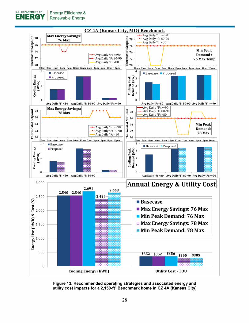
28

CZ 4A (Kansas City, MO) Benchmark

Figure 13. Recommended operating strategies and associated energy and utility cost impacts for a 2,150-ft2 Benchmark home in CZ 4A (Kansas City)

60

62

64

66

68

70

72

74

76

78


Ther

mos

tat S

etpo

int



0

1

2

3

4


Cool

ing

Peak

D

eman

d (k


60

62

64

66

68

70

72

74

76

78


Ther

mos

tat S

etpo


78 Max


0

1

2


Cool

ing

Ener

gy

(MW

h)

BasecaseProposed

60

62

64

66

68

70

72

74

76

78


Ther

mos

tat S

etpo


76 Max


0

1

2


Cool

ing

Ener

gy

(MW

h)

BasecaseProposed

60

62

64

66

68

70

72

74

76

78


Ther

mos

tat S

etpo

int

Min Peak Demand :

76 Max Temp


0

1

2

3

4


Cool

ing

Peak

D

eman

d (k

W)

Basecase Proposed

2,540

$352

2,540

$352

2,691

$356

2,424

$290

2,653

$305

0

500

1,000

1,500

2,000

2,500

3,000


Ener

gy U

se (k

Wh)

& C

ost (

$)



29

CZ 4A (Kansas City, MO) High Performance

Figure 14. Recommended operating strategies and associated energy and utility cost impacts for a 2,150-ft2 high performance home in CZ 4A (Kansas City)

60

62

64

66

68

70

72

74

76

78


Ther

mos

tat S

etpo

int



0

1

1

2

2

3


Cool

ing

Peak

D

eman

d (k


60

62

64

66

68

70

72

74

76

78


mos

tat S

etpo


78 Max


0

1


Cool

ing

Ener

gy

(MW

h)

BasecaseProposed

60

62

64

66

68

70

72

74

76

78


Ther

mos

tat S

etpo


76 Max


0

1


Cool

ing

Ener

gy

(MW

h)

BasecaseProposed

60

62

64

66

68

70

72

74

76

78


Ther

mos

tat S

etpo

int

Min Peak Demand :

76 Max Temp


0

1

1

2

2

3


Cool

ing

Peak

D

eman

d (k

W)

Basecase Proposed

1,454

$195

1,454

$195

1,719

$173

1,391

$154

1,549

$155

0

200

400

600

800

1,000

1,200

1,400

1,600

1,800

2,000


Ener

gy U

se (k

Wh)

& C

ost (

$)



30

CZ 5A (Boston, MA) Benchmark

Figure 15. Recommended operating strategies and associated energy and utility cost impacts for a 2,150-ft2 Benchmark home in CZ 5A (Boston)

60

62

64

66

68

70

72

74

76

78


Ther

mos

tat S

etpo

int



0

1

1

2

2

3


Cool

ing

Peak

D

eman

d (k


60

62

64

66

68

70

72

74

76

78


mos

tat S

etpo


78 Max


0

1


Cool

ing

Ener

gy

(MW

h)

BasecaseProposed

60

62

64

66

68

70

72

74

76

78


Ther

mos

tat S

etpo


76 Max


0

1


Cool

ing

Ener

gy

(MW

h)

BasecaseProposed

60

62

64

66

68

70

72

74

76

78


Ther

mos

tat S

etpo

int

Min Peak Demand :

76 Max Temp


0

1

1

2

2

3


Cool

ing

Peak

D

eman

d (k

W)

Basecase Proposed

721

$103

720

$103

1,062

$111

662

$73

801

$80

0

200

400

600

800

1,000

1,200


Ener

gy U

se (k

Wh)

& C

ost (

$)



31

CZ 5A (Boston, MA) High Performance

Figure 16. Recommended operating strategies and associated energy and utility cost impacts for a 2,150-ft2 high performance home in CZ 5A (Boston)

60

62

64

66

68

70

72

74

76

78


Ther

mos

tat S

etpo

int



0

1

1

2


Cool

ing

Peak

D

eman

d (k


60

62

64

66

68

70

72

74

76

78


Ther

mos

tat S

etpo


78 Max


0

1


Cool

ing

Ener

gy

(MW

h)

BasecaseProposed

60

62

64

66

68

70

72

74

76

78


Ther

mos

tat S

etpo


76 Max


0

1


Cool

ing

Ener

gy

(MW

h)

BasecaseProposed

60

62

64

66

68

70

72

74

76

78


Ther

mos

tat S

etpo

int

Min Peak Demand :

76 Max Temp


0

1

1

2


Cool

ing

Peak

D

eman

d (k

W)

Basecase Proposed

419

$59

419

$59

590

$59

390

$41

449

$45

0

100

200

300

400

500

600

700


Ener

gy U

se (k

Wh)

& C

ost (

$)



32

CZ 5B (Denver, CO) Benchmark

Figure 17. Recommended operating strategies and associated energy and utility cost impacts for a 2,150-ft2 Benchmark home in CZ 5B (Denver)

60

62

64

66

68

70

72

74

76

78


Ther

mos

tat S

etpo

int



01122334


Cool

ing

Peak

D

eman

d (k


60

62

64

66

68

70

72

74

76

78


Ther

mos

tat S

etpo


78 Max


0

1


Cool

ing

Ener

gy

(MW

h)

BasecaseProposed

60

62

64

66

68

70

72

74

76

78


Ther

mos

tat S

etpo


76 Max


0

1


Cool

ing

Ener

gy

(MW

h)

BasecaseProposed

60

62

64

66

68

70

72

74

76

78


Ther

mos

tat S

etpo

int

Min Peak Demand :

76 Max Temp


01122334


Cool

ing

Peak

D

eman

d (k

W)

Basecase Proposed

981

$149

969

$146

1,184

$151

880

$106

1,183

$121

0

200

400

600

800

1,000

1,200

1,400


Ener

gy U

se (k

Wh)

& C

ost (

$)



33

CZ 5B (Denver, CO) High Performance

Figure 18. Recommended operating strategies and associated energy and utility cost impacts for a 2,150-ft2 high performance home in CZ 5B (Denver)

60

62

64

66

68

70

72

74

76

78


Ther

mos

tat S

etpo

int



0

1

1

2

2


Cool

ing

Peak

D

eman

d (k


60

62

64

66

68

70

72

74

76

78


Ther

mos

tat S

etpo


78 Max


0

1


Cool

ing

Ener

gy

(MW

h)

BasecaseProposed

60

62

64

66

68

70

72

74

76

78


Ther

mos

tat S

etpo


76 Max


0

1


Cool

ing

Ener

gy

(MW

h)

BasecaseProposed

60

62

64

66

68

70

72

74

76

78


Ther

mos

tat S

etpo

int

Min Peak Demand :

76 Max Temp


0

1

1

2

2


Cool

ing

Peak

D

eman

d (k

W)

Basecase Proposed

532

$78

532

$78

770

$77

481

$53

584

$58

0

100

200

300

400

500

600

700

800

900


Ener

gy U

se (k

Wh)

& C

ost (

$)



DOE/GO-102014-4571 ▪ December 2014

buildingamerica.gov

Residential Mechanical Precoolingapps1.eere.energy.gov/buildings/publications/pdfs/... ·...

Documents

Transcript of Residential Mechanical Precoolingapps1.eere.energy.gov/buildings/publications/pdfs/... ·...