RESEARCH ROADMAP FOR GREENHOUSE GAS INVENTORY

METHODS

Prepared For: California Energy Commission

Prepared By: University of California, Berkeley Lawrence Berkeley National Laboratory California Energy Commission

CO

NSU

LTA

NT

REP

OR

T

July 2005

CEC-500-2005-097

Prepared By: Alexander E. Farrell

Amber C. Kerr Adam R. Brandt University of California, Berkeley

Margaret S. Torn Lawrence Berkeley National Laboratory

Guido Franco California Energy Commission, PIER Energy-Related Environmental Research

Contract No. 700-99-019 Work Authorization 15 Prepared For:

California Energy Commission Gina Barkalow, Contract Manager Guido Franco, Project Manager Kelly Birkinshaw, Program Area Team Lead PIER ENERGY-RELATED

ENVIRONMENTAL RESEARCH Martha Krebs, Ph.D., Deputy Director ENERGY RESEARCH AND

DEVELOPMENT DIVISION B. B. Blevins Executive Director

DISCLAIMER This report was prepared as the result of work sponsored by the

California Energy Commission. It does not necessarily represent the views of the Energy Commission, its employees or the State of California. The Energy Commission, the State of California, its employees, contractors and subcontractors make no warrant, express or implied, and assume no legal liability for the information in this report; nor does any party represent that the uses of this information will not infringe upon privately owned rights. This report has not been approved or disapproved by the California Energy Commission nor has the California Energy Commission passed upon the accuracy or adequacy of the information in this report.

i

Acknowledgments The authors and PIER would like to thank the following individuals, and those listed under Section 10 (Contacts), for their help in preparing this document:

• Pascale Boeckx, Ghent University, Belgium • Jean Bogner, Landfill +, Inc • Anne Choate, ICF Consulting • Mark Conrad, Lawrence Berkeley National Laboratory • Marc Fischer, Lawrence Berkeley National Laboratory • Changsheng Li, University of New Hampshire • Arvin Mosier, USDA/ARS, Fort Collins, Colorado • Jos Olivier, RIVM (viz. the Dutch Ministry of Environment) • Lynn Price, Lawrence Berkeley National Laboratory • Diana Pape, ICF Consulting • Riitta Pipatti, IPCC Task Force on National Greenhouse Gas Inventories • Dennis Rolston, University of California, Davis • William Riley, Lawrence Berkeley National Laboratory • William Salas, Applied Geosolutions, Inc., Durham, New Hampshire • Alan Sanstad, Lawrence Berkeley National Laboratory • Jayant Sathaye, Lawrence Berkeley National Laboratory • Susan Thorneloe, U.S. Environmental Protection Agency • Fabian Wagner, IPCC Task Force on National Greenhouse Gas Inventories • Wilfried Winiwarter, International Institute for Applied Systems Analysis, Austria

ii

Table of Contents

Acknowledgements.......................................................................................................................... i Executive Summary .........................................................................................................................1 Roadmap Organization ....................................................................................................................3 1. Issue Statement ....................................................................................................................... 4 2. Public Interest Vision.............................................................................................................. 4 3. Background............................................................................................................................. 4

3.1 Principal Literature Sources for Inventory Methodologies ............................................ 5 3.2 Methods of Calculating Emissions Inventories .............................................................. 6 3.3 Global Warming Potential .............................................................................................. 9 3.4 Overview of GHG Emissions from California ............................................................. 10

3.4.1. Greenhouse Gas Sinks .......................................................................................... 12 3.5 Prioritization of GHG Inventory Research ................................................................... 13

3.5.1. Key Sources .......................................................................................................... 13 3.5.2. Emissions Uncertainty .......................................................................................... 13 3.5.3. Uncertainty in Global Warming Potential ............................................................ 14 3.5.4. Potential for Improvement .................................................................................... 14

3.6 The PIER Focus ............................................................................................................ 15 3.7 Potential Methods to Improve GHG Emissions Estimates ........................................... 15

4. Current Research and Research Needs ................................................................................. 16 4.1 Carbon Dioxide (CO2) .................................................................................................. 16

4.1.1. Carbon Dioxide from the Combustion of Fossil Fuels ......................................... 16 4.2 Methane (CH4) .............................................................................................................. 21

4.2.1. Landfills ................................................................................................................ 22 4.2.2. Enteric Fermentation............................................................................................. 39 4.2.3. Manure Management ............................................................................................ 50 4.2.4. Natural Gas Systems ............................................................................................. 57 4.2.5. Methane Emissions from Wastewater .................................................................. 62

4.3 Nitrous Oxide (N2O) ..................................................................................................... 66 4.3.1. Agricultural Soils .................................................................................................. 67 4.3.2. Mobile Source Combustion (Vehicles)................................................................. 82 4.3.3. Wastewater............................................................................................................ 86

4.4 High-GWP Gases: Fluorocarbons (HFCs, PFCs) and Sulfur Hexafluoride (SF6)........ 90 4.4.1. Substitution of Ozone Depleting Substances........................................................ 91 4.4.2. Semiconductor Manufacture................................................................................. 94 4.4.3. Electric Utilities .................................................................................................... 97

4.5 Tropospheric Ozone and Aerosols.............................................................................. 101 4.5.1. Ozone .................................................................................................................. 101 4.5.2. Aerosols .............................................................................................................. 104

4.6 Inverse Modeling ........................................................................................................ 105 5. Goals ................................................................................................................................... 107 6. Leveraging R&D Investments ............................................................................................ 109

6.1 Opportunities for Leverage within the CEC PIER Program....................................... 109 6.2 Opportunities for Leverage with Other Programs ...................................................... 109

iii

7. Areas Not Addressed by This Roadmap............................................................................. 111 7.1 Gas/activity Combinations Not Covered .................................................................... 111

8. References........................................................................................................................... 112 9. Acronyms............................................................................................................................ 124 10. Contacts........................................................................................................................... 125

10.1 Landfills ...................................................................................................................... 125 10.2 Enteric Fermentation................................................................................................... 126 10.3 Manure Management .................................................................................................. 127 10.4 Natural Gas ................................................................................................................. 128 10.5 Wastewater.................................................................................................................. 128 10.6 Agricultural Soils ........................................................................................................ 128 10.7 Substitution of Ozone Depleting Substances.............................................................. 130 10.8 Semiconductor Manufacturing.................................................................................... 130 10.9 Electric Utilities .......................................................................................................... 131

List of Figures Figure 3-1. Percent contribution to increased radiative forcing, 1750–2000 ............................... 10 Figure 3-2. Percent emissions of CH4 and N2O in California by sector, 1999 (CO2-eq.)............ 11 Figure 3-3. The 2002 U.S. greenhouse gas inventory and uncertainty estimate (MMT CO2-eq.).

The height of the column shows the expected value. The bars show ±2.5% confidence limits and thus delineate the 95% confidence interval for that gas/activity sector’s inventory (EPA 2004). .................................................................................................................................... 14

Figure 4-1. Various fuels’ contribution to total California CO2 emissions from the combustion of fossil fuels, 1999 ................................................................................................................... 17

Figure 4-2. Changes in GHG emissions from various fuels in California.................................... 19 Figure 4-3. Schematic of methane emissions from landfills, including production, oxidation,

recovery and flaring .............................................................................................................. 23 Figure 4-4. Contribution of different livestock types to enteric methane in California in 1999. 39 Figure 4-5. Parameters required to estimate enteric methane production in IPCC

methodology ......................................................................................................................... 41 Figure 4-6. Contribution of different livestock types to methane from manure management in

California, 1999. ................................................................................................................... 51 Figure 4-7. Major sources of nitrous oxide emissions in California, 1999.................................. 67 Figure 4-8. Effect of soil oxygen saturation on N2O production................................................. 68 Figure 4-9. A “leaky pipe” diagram of microbial N2O production............................................... 69 Figure 4-10. N2O production through direct and indirect emissions from agricultural soils ....... 71 Figure 4-11. Sources of N2O from wastewater............................................................................ 86

iv

List of Tables Table 3-1. Key sources for GHG inventory methods ..................................................................... 6 Table 3-2. Relative comparison of emission factor and process models. This table draws on the

typical characteristics of the models, but exceptions exist in almost every category............ 8 Table 3-3. Global warming potential of selected greenhouse gases as reported in the IPCC Third

Assessment Report (TAR) ...................................................................................................... 9 Table 3-4. Contribution of California to U.S. greenhouse gas emissions, 1999........................... 10 Table 3-5. Sources of non-CO2 GHGs in California. Inventory units are MMT CO2 eq............ 12 Table 4-1. Methane sources and emission rates in California ..................................................... 22 Table 4-2. Uncertainties in IPCC parameters used to estimate methane emissions from landfills

(default and FOD methods) .................................................................................................. 28 Table 4-3. Methods for measuring methane emissions and methane oxidation in landfills......... 32 Table 4-4. Summary of research needs: Landfill methane emissions ........................................ 38 Table 4-5. Data needed for each livestock subgroup in IPCC Tier 2 method for estimating

methane from enteric fermentation....................................................................................... 41 Table 4-6. Partial list of methane conversion factors (Ym) currently used by EPA (2004) and

IPCC (2000a) ........................................................................................................................ 43 Table 4-7. Uncertainty bounds on IPCC estimates of Ym (methane conversion factor for enteric

fermentation)......................................................................................................................... 47 Table 4-8. Summary of empirical techniques for characterizing livestock enteric methane

emissions............................................................................................................................... 49 Table 4-9. Default methane conversion factors (MCFs) for manure management systems by

climate................................................................................................................................... 52 Table 4-10. Emission factors for methane from natural gas systems, ICF/EIIP method.............. 59 Table 4-11. Summary of research needs for wastewater emissions of methane .......................... 66 Table 4-12. Factors controlling soil N2O production................................................................... 70 Table 4-13. Default values and uncertainty ranges of IPCC emission factors for N2O production

from agricultural soils ........................................................................................................... 74 Table 4-14. Some ecosystem process models for predicting N2O flux from soils ...................... 76 Table 4-15. Summary of research needs for N2O emissions from agricultural soils................... 82 Table 4-16. GWP weighted emissions of high-GWP gases, California 1999 .............................. 90 Table 4-17. Research needs for high-GWP gases...................................................................... 101 Table 5-1. Prioritized research goals for GHG inventory improvement .................................... 108 Table 7-1. Gas/activity combinations not covered ..................................................................... 111

1

Executive Summary Anthropogenic activities in California are a globally significant source of greenhouse gas (GHG) emissions, which are the primary cause of climate change. The California legislature mandates the state to inventory California’s GHG emissions every five years. Improvements in inventory methodologies are needed. Priorities for research were assessed by taking into account source strength, inventory quality, and the near-term potential for improving inventory methods. Improvements realized through the program should benefit the U.S. Environmental Protection Agency (EPA) and other national inventory efforts. The Public Interest Energy Research Environmental Area (PIER-EA) has identified nine priority areas of research to improve California's greenhouse gas inventory: (1) agricultural soils nitrous oxide (N2O), (2) landfill methane (CH4), (3) high-global warming potential gases, (4) enteric fermentation CH4, (5) secondary pollutants, (6) manure management CH4 and N2O, (7) inverse methods, (8) wastewater CH4 and N2O, and (9) mobile N2O. The suggested research includes better evaluations and characterizations of existing data; collecting new data; and developing improved processes, methods, models, and inventories. These recommendations are identified in the accompanying table and are further detailed in the report. The successful completion of the activities noted in the report will help California improve the methods used to estimate the state's GHG emissions and should result in more accurate accounting of those emissions. The products from this research can be used by the California Energy Commission to improve the statewide inventory that it is mandated to produce every five years. The Public Interest Energy Research (PIER) climate change research plan1 also identifies mid-term (3–10 year) and long-term (10–20 year) goals, all of which build on the short-term work. This roadmap outlines a comprehensive research agenda that would be necessary to fully address the research gaps identified here. However, due to the limited funding, PIER will be able to support only some of the identified areas of research. Currently, PIER is examining all of the roadmaps to determine which projects should be supported with PIER funding.

1 California Energy Commission. April 2003. PIEREA Climate Change Research, Development, and Demonstration Plan. Public Interest Energy Research (PIER) Program. 500-03-025FS.

2

Prioritized research goals for GHG inventory improvement Priority 1. Agricultural Soils Nitrous Oxide Short • Compare existing IPCC, ecosystem model, and measured estimates by county and land use. Med • Measure N2O emissions from range of agricultural soils.

• Develop multi-factor EF model or nitrogen ecosystem model for inventory. Long • Implement C/N ecosystem model for Land Use Change and nitrogen inventories.

• Begin regional nitrogen budget and estimates of indirect N2O emissions. Priority 2. Landfill Methane Short • Measure landfill methane emissions and improve existing emission factor model. Med • Determine landfill waste characteristics and waste generation and landfilling rates.

• Develop function relating gas recovery to production. Long • Develop simple process level model of oxidation.

• Synthesize improved model of net emissions. Priority 3. High-GWP Gases Short • Use industry sector approach to develop “bottom up” inventory, using EPA methodology. Med • Improve emission factors for bottom up inventory (varies by gas).

Long • Apply inverse methods to verify inventory. Priority 4. Enteric Fermentation Methane Med • Reduce uncertainty in methane conversion factor (Ym) for cattle populations in California.

Priority 5. Secondary Pollutants Short • Evaluate methods of inventorying precursors to tropospheric ozone and aerosols. Long • Investigate the potential value of developing methods to relate emissions to climate forcing.

Priority 6. Manure Management Methane and Nitrous Oxide Short • Collect activity data for manure management systems. Med • Compare measurements of methane and N2O emissions to IPCC estimate.

Priority 7. Inverse Methods Short • Identify promising applications, key measurements, and possible partners. Med • Apply inversion methods to non-CO2 GHG, leverage existing data.

Long • Reconcile “top down” and “bottom up” inventories. • Focus on N2O from indirect emissions and high-GWP gases.

Priority 8. Wastewater Methane and Nitrous Oxide Med • Develop regression of emissions on BOD using California data.

Priority 9. Mobile Nitrous Oxide Med • Reduce the uncertainties associated with activity data. Med • Develop method to integrate cold starts into emissions inventory. Med • Improve emission factors for heavy-duty vehicles, including emission controls.

3

Roadmap Organization This roadmap is intended to communicate to an audience that has moderate technical acquaintance with the issue. The sections build upon each other to provide a framework and justification for the proposed research and development. Section 1 states the issue to be addressed. Section 2: Public Interest Vision provides an overview of research needs in this area and how PIER plans to address those needs. Section 3: Background establishes the context of PIER’s climate change work in the area of greenhouse gas inventories. Section 4: Current Research and Research Needs surveys current inventory methods and identifies specific research needs that are not already being addressed by current projects. Section 5: Goals outlines proposed activities that will meet those needs. Section 6: Leveraging R&D Investments identifies methods and opportunities to help ensure that the investment of research funds will achieve the greatest public benefits. Section 7: Areas Not Addressed by this Roadmap identifies topics related to climate change research that the proposed activities do not address. Section 8: References identifies the references used for this roadmap. Section 9: Acronyms identifies the acronyms used in the roadmap. Section 10: Contacts provides contact information for those who were consulted for the development of this roadmap. Totals in the tables of this roadmap may not be exact, due to rounding of some of the data.

4

1. Issue Statement There is a need to improve our understanding of the emissions and sinks of greenhouse gases (GHG) in the State of California, to improve the accuracy of the statewide inventory that the California Energy Commission is mandated to produce every five years.

2. Public Interest Vision The primary mission of the California Energy Commission’s Public Interest Energy Research (PIER) program is to conduct research that helps deliver “environmentally sound, safe, reliable, and affordable electricity” to California citizens. The mission of PIER’s Environmental Area (PIER-EA) is “to develop cost-effective approaches to evaluating and resolving environmental effects of energy production, delivery, and use in California, and explore how new electricity applications and products can solve environmental problems.” The Public Interest Energy Research Environmental Area (PIER-EA) has identified nine priority areas of research to improve California's greenhouse gas inventory: (1) agricultural soils nitrous oxide (N2O), (2) landfill methane (CH4), (3) high-global warming potential gases, (4) enteric fermentation CH4, (5) secondary pollutants, (6) manure management CH4 and N2O, (7) inverse methods, (8) wastewater CH4 and N2O, and (9) mobile N2O. The suggested research includes better evaluations and characterizations of existing data; collecting new data; and developing improved processes, methods, models, and inventories. These recommendations are identified in the accompanying table and are further detailed in the report. The successful completion of the activities noted in the report will help California improve the methods used to estimate the state's GHG emissions and should result in more accurate accounting of those emissions. The products from this research can be used by the California Energy Commission to improve the statewide inventory that it is mandated to produce every five years.

3. Background There is broad scientific consensus that rising concentrations of GHGs in the atmosphere will lead to global climate change in this century (IPCC 2001). In response to the threats posed by climate change, over 180 nations, including the United States, have ratified the United Nations Framework Convention on Climate Change (UNFCCC). In doing so, nations agree to report the magnitude and sources of their GHG emissions and sinks (i.e., to produce a GHG inventory). In addition, they report activities undertaken to reduce emissions and enhance sinks. Carbon dioxide (CO2) is the GHG responsible for the most change in climate forcing over the past 150 years. The UNFCCC identifies five primary non-CO2 greenhouse gases: CH4, N2O, hydrofluorocarbons (HFCs), perfluorocarbons (PFCs), and sulfur hexafluoride (SF6)—the last three known collectively as halocarbons or high global warming potential gases (high-GWP gases). Within the UNFCCC framework, the Intergovernmental Panel on Climate Change (IPCC) issues authoritative guidelines for UNFCC reporting.

5

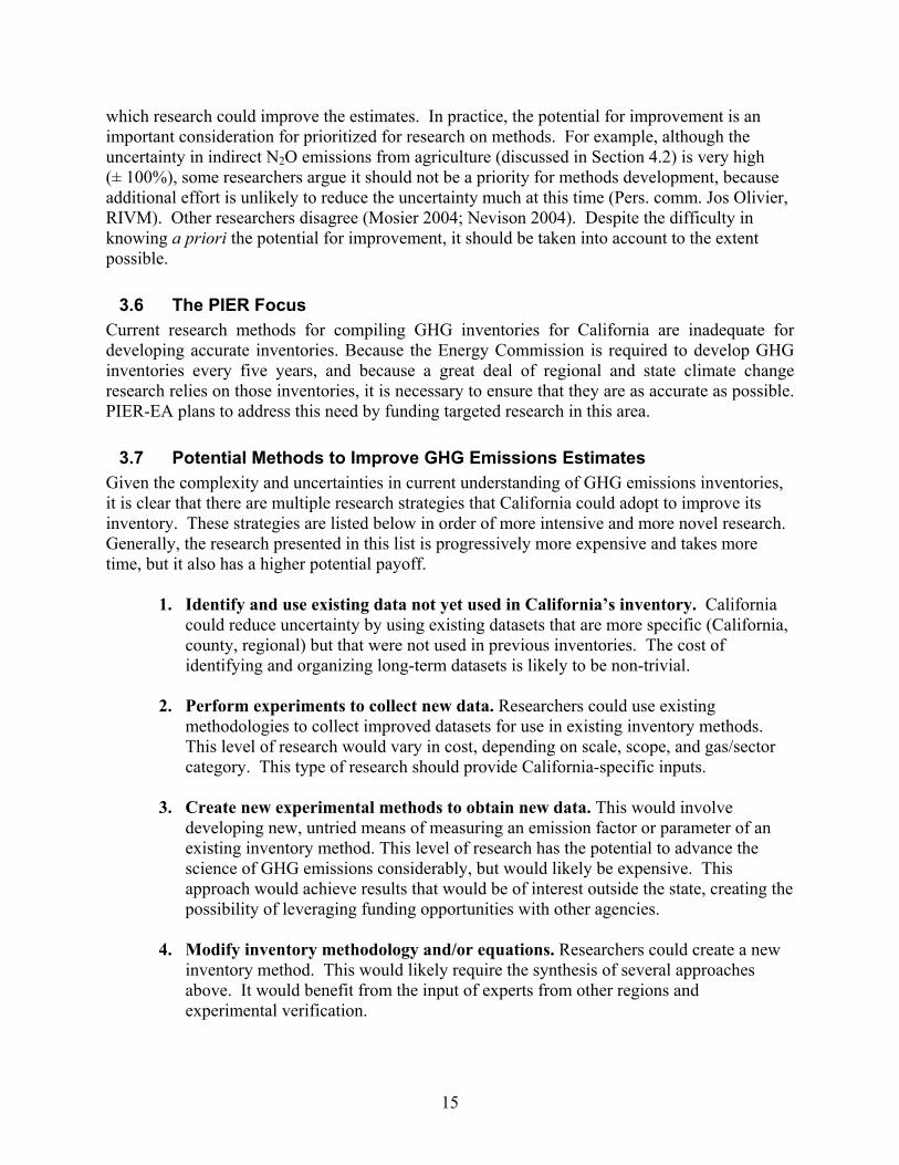
Within this context, the California legislature mandated that the state produce its own GHG inventory (SB 1771, Sher, Chapter 1018, Statutes of 2000). This law requires the California Energy Commission (Energy Commission), in consultation with other state agencies, to update California’s inventory of GHG emissions every five years, starting in 2002. Unfortunately, emissions inventories for most GHGs are highly uncertain, due to limitations in inventory methods and data availability. Obtaining an accurate inventory is important for several reasons: to evaluate mitigation options, predict emissions, to set the stage for various control strategies (including market-based instruments), and to assist in national reporting requirements. The first (and most recent) California inventory report, Inventory of California Greenhouse Gas Emissions and Sinks: 1990–1999 (referred to herein as the 2002 California GHG Inventory), concluded that there were major uncertainties associated with input data quality, protocols available to disaggregate data, and inventory methodologies applied to the state (CEC 2002). It recommended that future GHG inventories could be improved by: (1) incorporating improved data and methods; (2) updating emissions estimates to the most recent year; and (3) presenting a discussion of the uncertainty in emissions estimates from key sources. The goal of the roadmap presented here is to respond to the first of these recommendations by identifying priorities and opportunities for research that would improve the inventory data and methods used in the state. This roadmap considers research to improve inventory methodologies for the five important non-CO2 greenhouse gases and particulates—CH4, N2O, fluorine-containing industrial gases, ozone (O3), and aerosols—and focuses on anthropogenic sources, as required by IPCC guidance. For example, the roadmap considers methane flux from landfills but not from wetlands. Greenhouse gas inventories are typically conducted on the basis of gas-activity pairs; that is, the emissions of a particular gas are given for a specific activity. For instance, methane from wastewater treatment is inventoried separately from methane from landfills, and separately from nitrous oxide from wastewater treatment. This roadmap adopts this gas-activity approach as well.

3.1 Principal Literature Sources for Inventory Methodologies Several guidance documents for conducting GHG inventories have been developed. Five of the most important for California are shown in Table 3-1. The Revised 1996 IPCC Guidelines for National Greenhouse Gas Inventories (herein referred to as the IPCC Guidelines) (IPCC 1997) describe the emission inventory process at the most basic level, and, as a global reference, must provide methods suitable for all types of nations, industrialized and developing. A closely related report, Good Practice Guidance and Uncertainty Management in National Greenhouse Gas Inventories (IPCC 2000a) provides further guidance on improved methods. The IPCC inventory methods for each gas-activity pair are stratified into tiers by the intensity of data requirements and model complexity. The Tier 1 methods are the simplest, and include default parameters so that a minimum of country-specific data are required. Tier 2 methods are more data intensive; they may involve the application of more country-specific parameters to Tier 1 methods. Tier 3 methods are the most complex, commonly involving detailed datasets collected at the national level. Research is underway under the IPCC National Greenhouse Gas Inventories Programme (IPCC-NGGIP) to continue to develop and refine internationally agreed methodologies and software for the calculation and reporting of national GHG emissions and removals.2

2 See http://www.ipcc-nggip.iges.or.jp/index.html.

6

The United States Environmental Protection Agency (EPA) produces an annual Inventory of U.S. Greenhouse Gas Emissions and Sinks, which includes information on national methodologies in the Annexes to these reports (EPA 2003b). Generally, the IPCC guidance documents recommend that states use these national methods where they exist. In addition, the EPA also funded the development of a simplified set of inventory methods for use by individual states, which are published as part of the Emission Inventory Improvement Program (EIIP). The most recent version of the EIIP was published in 1999 and in addition the draft 2003 EIIP was made available to the authors of this report. The current 2002 California GHG Inventory (CEC 2002) used a variety of methods based on IPCC, EPA, or EIIP guidance, and some were adapted for California-specific data or methods. For this review, researchers examined all of the guidance documents shown in Table 3-1. Current efforts to revise the IPCC and EPA methodologies for non-GHG inventories are under way but not yet available (pers. comm. Fabian Wagner and Riitta Pipatti (IPCC Task Force on National Greenhouse Gas Inventories) and Andrea Denny (EPA)).

Table 3-1. Key sources for GHG inventory methods 1. IPCC (1997). Revised 1996 IPCC Guidelines for National Greenhouse Gas Inventories: Reporting

Instructions. Intergovernmental Panel on Climate Change, IPPC XII (Mexico City), September 1996.

2. IPCC (2000). Good Practice Guidance and Uncertainty Management in National Greenhouse Gas Inventories. Intergovernmental Panel on Climate Change, National Greenhouse Gas Inventories Programme, Montreal, IPCC XVI/Doc. 10 (1.IV.2000), May 2000.

3. EPA (2004). Inventory of U.S. Greenhouse Gas Emissions and Sinks: 1990-2002. U.S. Environmental Protection Agency, Washington DC, EPA 430-R-02-03, April 2002.

4. EIIP (1999). EIIP Volume VIII: Estimating Greenhouse Gas Emissions. Emission Inventory Improvement Program (U.S. Environmental Protection Agency), Technical Report Series, October 1999

5. CEC (2002). Inventory of California Greenhouse Gas Emissions and Sinks: 1990-1999. California Energy Commission, Sacramento, California. Publication #600-02-001F, November 2002.

3.2 Methods of Calculating Emissions Inventories Methods for calculating emissions inventories lie along a spectrum of complexity between two endpoints: (1) emission factor (EF) models, and (2) process models (NRC 2003). Inventory methods generally increase in complexity from EF models to process models, although there is not always a clear distinction between them. (The term “multi-factor models” is sometimes used to refer to approaches in between the two ends of the spectrum.) Regression analyses are often used in the development of models and model parameters, especially for EF models. At the one end of the spectrum, EF models often use a single factor to estimate emissions of a gas from a specific activity, such as N2O emissions per vehicle mile traveled. The distinguishing feature of the EF approach is a reliance on activity data, or measurements of relevant actions. For instance, in a very basic emission factor model, annual emissions of N2O from a typical car might be multiplied by the number of cars in the country to calculate national emissions. The accuracy of EF methods can be improved by disaggregating the activity data into activity sub-types, and applying specific emission factors to each sub-type. This can be done, for instance, by differentiating between passenger cars and large trucks, or gasoline and diesel autos. An

7

emission factor model typically has the form shown in Equation 3-1, although not all emission factor models involve this level of disaggregation:

Emissions = EFa,b,c × Activitya,b,ca,b,c∑ Equation 3-1

where:

EF = emission factor (e.g., grams/mile traveled) Activity = activity level measured in the units appropriate for the emission factor

(e.g., vehicle miles traveled) a = activity type A (e.g., fuel type) b = activity type B (e.g., vehicle type) c = activity type C (e.g., emission control type)

The principal advantage of the EF approach is its simplicity—few types of data are needed and the data are usually selected to be relatively easy to obtain. The main difficulty is in defining a small set of “typical” activity factors, especially for emissions that occur under, and are sensitive to, widely varying conditions. Most inventory methods include one or more corrections to compensate for a process, even if the basic form of the method is an EF model. For example, the process of methane oxidation in landfill soils is taken into account by subtracting a fixed percentage of the emission generated by the emission factor model. At the other end of the spectrum are process models (also called simulation or mechanistic models). These models attempt to represent the underlying biophysical processes that cause the emissions of GHGs. They often include parameters determined experimentally, not statistically. Process models often involve decay parameters to model temporal variation, or temperature-dependent equations that represent the temperature-governed activity of microorganisms. Process models attempt to represent the main processes leading to net emission, and to the extent possible (or useful), are built from fundamental principles such as conservation of mass and chemical reaction kinetics. For instance, for landfill methane, relevant processes include methane production from digestible waste in place, gas recovery, and methane oxidation. Process models are usually more detailed than EF models, and typically provide more insight into the mechanisms by which emissions occur. Process-based models may also be better tools for evaluating the impact of management and climate variability, and the effectiveness of mitigation strategies. However, they are typically also more demanding in terms of cost to develop, and most require more input data than do EF models. There are important choices among these model types in creating a GHG inventory research strategy. Factors that guide the choice of models include accuracy, cost, ability to be validated, and ability to predict emissions over a range of conditions. These factors are not always exclusive and are not always linked to one type of model. For example, process models are not always more accurate than EF models. Different institutions may place different weight on these factors, so greater accuracy may not always be worth increased cost. Thus, for instance,

8

implementing a process model for part of a statewide inventory might be considered cost-prohibitive, while the development of process models in order to improve EFs used for inventories might not. Another example involves, validation, a critical need for any inventory method; a process model could be considered a cost-effective means of validating or improving an EF model, especially if the process model can help show how an EF model can be simplified while still retaining adequate accuracy and reliability. For instance, a process model might show that accuracy of an EF model can be maintained by using three readily obtainable factors instead of one hard-to-obtain factor, allowing for a less expensive inventory process. Some of the advantages and disadvantages of these two types of methods are outlined in Table 3-2.

Table 3-2. Relative comparison of emission factor and process models. This table draws on the typical characteristics of the models, but exceptions

exist in almost every category.

Type of model

Ease of

use

Limited data

inputs required

to use

Less expensive

or time consuming to develop

Require validation

Accurate in local or historical context

Appropriate outside

original range of input data

Include variables for evaluating

climate or management

scenarios

Emission factors X X X X X

Process-based X X X X

It should be noted that the term regression models is often used when referring to EF models. This somewhat confusing terminology arises because, even though EF models are not, strictly speaking, regression models, emission factors are often created through the use of regression analysis. A novel, emerging approach to improving GHG inventories is to use atmospheric concentration measurements and a transport model to estimate the total source strength of a GHG from a region, known as inverse modeling. These “top-down” results can be used as a constraint on an inventory estimated by traditional means. For example, the inverse approach using N2O concentrations would give the total N2O flux, from natural and anthropogenic sources combined, from a region, and thus would form an upper bound on the amount of N2O flux from any or all anthropogenic sources. Inverse modeling may never replace traditional, “bottom up” methods because it cannot distinguish different sources if they are located near each other. It also will not offer large improvements if the uncertainties in the inversion model are similar to, or larger than, the uncertainties in the bottom up estimates. For example CO2 inventories are known to better than 5% uncertainty. But for inventories that are highly uncertain—which includes all the non-CO2 gases—the “top down” methods may offer an important means of verifying or even improving the inventory. In addition, in some cases, anthropogenic and natural sources can be distinguished using isotopes or elemental ratios. Although inverse modeling could be applied separately to each GHG in the inventory, it is discussed separately, in Section 4.6.

9

3.3 Global Warming Potential Not all GHGs have the same effectiveness; emitting a ton of one GHG will have a different effect on climate than emitting a ton of another. Emitting GHGs tends to increase their concentrations in the atmosphere, which tends to make the atmosphere absorb more of the incoming solar radiation, thus raising the temperature of the atmosphere. This effect is called “radiative forcing” and leads to climate change. A positive radiative forcing tends to warm the surface of the Earth, and negative forcing tends to cool the surface. Gases differ in their warming potential for three reasons: (1) the direct radiative forcing of the molecule; (2) the atmospheric lifetime of the gas; and (3) the indirect radiative forcing, which can come about due to changes to atmospheric chemistry brought on by increasing concentrations of the gas in the atmosphere. To compare the radiative forcing of emissions of different species, the Global Warming Potential (GWP) unit was created. The GWP is the cumulative radiative forcing over a specified time span caused by the emission of a unit mass of gas, relative to emission of a reference gas (IPCC 2001). The reference gas is CO2 which thus has a GWP of 1. In contrast, a molecule of SF6 is thousands of times more effective at absorbing and reradiating infrared radiation than CO2 for any given period, and each emitted SF6 molecule stays in the atmosphere much longer, resulting in a GWP for SF6 of 22,200 (IPCC 2001). The parties to the UNFCCC currently use GWPs based on a 100-year time horizon. Therefore, in this roadmap, emissions are expressed as GWP-weighted emissions in millions of metric tons of carbon dioxide equivalent (MMT CO2 Eq.), which is the same as teragrams of CO2 equivalent (Tg CO2 Eq.), for a 100-year time period. Although parties to the UNFCCC currently use GWP factors from the Second Assessment Report (SAR) (IPCC1995), these factors were slightly revised in the IPCC Third Assessment Report (TAR) (IPCC 2001), as a result of new laboratory or radiative transfer results, and the revised values are shown in Table 3-3.

Table 3-3. Global warming potential of selected greenhouse gases as reported in the IPCC Third Assessment Report (TAR)

Gas GWP † Lifetime (y) Molecular weight (g/mole)

CO2 1 NR 44 CH4 23 12 16 N2O 296 14 44 HFC-23 12,000 260 70 HFC-134a 1,300 13.8 102 HFC-152a 120 1.4 66 CF4 5700 50,000 88 SF6 22,200 3200 146 Tropospheric O3 NR 0.01-0.05 48

† Million metric tons of CO2 equivalent over 100 year integration time (MMT CO2 Eq.). NR = not reported in TAR because highly contingent (CO2) or not established (O3). Source: IPCC 2001.

10

3.4 Overview of GHG Emissions from California California is a major contributor to the U.S. GHG inventory of all gases, as shown in Table 3-4; therefore, efforts to improve California’s inventory will improve the quality of the national inventory as well.

Table 3-4. Contribution of California to U.S. greenhouse gas emissions, 1999 Gas U.S. total

(MMT CO2-eq.) U.S. (%)

CA total (MMT CO2-eq.)

CA (%)

CA (as % of U.S.)

CO2 5,666 83.0 362.8 84.8 6.4 CH4 621 9.1 31.7 7.4 5.1 N2O 424 6.2 23.6 5.5 5.6

High-GWP gases 120 1.8 9.7 2.3 8.1 Total 6,830 100 427.7 100 6.3 (avg.)

Sources: U.S. data is from EPA 2003b, and the California data is from CEC 2002. Some important influences on radiative forcing, and therefore on global warming, are excluded by examining only the gases included in Table 3-4. This is illustrated by Figure 3-1, which shows the increase in cumulative change in radiative forcing between 1750 and 2000 caused by five categories of atmospheric gases, on a global basis (IPCC 2001). Tropospheric ozone (O3) is the third most important GHG; increases in global background ozone account for about 13% of the total historical change in radiative forcing (albeit with large uncertainty in the underlying data). In addition, aerosols (i.e., liquid or solid particles suspended in the air) have significant impacts on climate, but are not included in Table 3-4.

Source: (IPCC 2001)

Figure 3-1. Percent contribution to increased radiative forcing, 1750–2000

The main reason that these species are not included is that tropospheric ozone and many aerosols are secondary pollutants (i.e., formed by chemical reactions in the atmosphere from primary pollutants, which are precursors that are directly emitted). They are short-lived and spatially variable GHGs, for which there are no agreed-upon methods for estimating the GWP of the precursors, or for accounting for the indirect effects of changes in tropospheric chemistry (IPCC 2001 pp. 277–279, 391). Nonetheless, IPCC requests that countries party to the UNFCCC report their emissions of ozone precursors. Accordingly, the U.S. inventory reports emissions of NOX,

11

and non-methane volatile organic compounds (NMVOCs) (EPA 2004). Because no GWP value is available for ozone precursors, inventories for them are given in mass of each gas, not mass of CO2-equivalent, and uncertainties are not calculated. For the gases that are included in the 2002 California GHG Inventory, there are more than 20 different gas-activity combinations in California’s non-CO2 GHG inventory. This roadmap covers the eleven sources that make up over 95% of California’s non-CO2 greenhouse gas emissions, as shown in Table 3-5. Figure 3-2 shows the relative contribution of individual activities to the state’s N2O and CH4 inventories. This roadmap covers 94% of California’s CH4 and N2O emissions, and 100% of emissions of high-GWP gases.

Figure 3-2. Percent emissions of CH4 and N2O in California by sector, 1999 (CO2-eq.)

Because of differences in economy, climate, and lifestyle, the relative importance of various gases and activities to the state’s inventory is different from that of the United States or world. For example, the three largest sources of non-CO2 GHG in the United States are N2O from agricultural soils, CH4 from waste disposal landfills, and CH4 from natural gas systems respectively; whereas in California, enteric fermentation ranks third, as shown in Table 3-5. As a

Agricultural Soils*

Mobile Source*

Wastewater*

Manure

Stationary Source

Nitric Acid

Agricultural Burning

Waste Combustion

Landfills*

Enteric*

Manure*

Natural Gas*

Wastewater*

Stationary Source

Rice

Mobile Source

Oil System

Agricultural Burning

(a) CH4

(b) N2O

* Indicates a sector covered by this report. Source: (CEC 2002).

12

comparison to an industrialized, European country, the top three sources in the Netherlands are: (1) CH4 from waste disposal, (2) N2O from agriculture, and (3) N2O from industrial processes (Olivier et al. 2003). Globally, the four most important sources of CH4 are: (1) energy (natural gas, coal mining, petroleum processing, and fossil fuel combustion; which account for 30% of anthropogenic emissions), (2) enteric fermentation (20%), (3) rice paddies (13%), and (4) landfills (13%); whereas in California, energy and rice paddies together account for less than 8% of the state’s CH4 emissions. As a result, this roadmap may prioritize different inventory methods than would be selected for areas outside of California.

Table 3-5. Sources of non-CO2 GHGs in California. Inventory units are MMT CO2 eq.

GHG Activity Calif. inventory and percentage

Calif. Rank

U.S. inventory and rank

N2O Agricultural Soils 14.7 (23%) 1 298 (1) CH4 Landfills 13.2 (20%) 2 204 (2) CH4 Enteric Fermentation 7.1 (11%) 3 117 (4)

High-GWP gases Ozone Depleting Substance Substitutes 7.0 (11%) 4 51 (5) N2O Mobile Source Combustion 6.2 (10%) 5 59 (7) CH4 Manure Management 5.2 (8%) 6 39 (8) CH4 Natural Gas System 2.9 (5%) 7 120 (3)

High-GWP gases Electric Utilities 1.9 (3%) 8 16 (15) CH4 Wastewater 1.4 (2%) 9 29 (10) N2O Human Sewage 1.1 (2%) 10 9 (16)

High-GWP gases Semiconductors 0.8 (1%) 11 7 (18) SUBTOTAL 61.5 (95.5%)

Other 2.9 (4.5%) TOTAL 64.4 (100%)

Notes: The values in this table vary somewhat with similar values for the United States as a whole. The sixth-ranked national source is methane from coal mining, and the ninth-ranked is high-GWP gases from HCFC-22 production. The EPA source includes industrial wastewater treatment in its wastewater category, whereas the Energy Commission source does not, so for the Energy Commission, wastewater and human sewage are identical activities. Sources: CEC 2002, p. 19; EPA 2003b.

3.4.1. Greenhouse Gas Sinks Human activities can enhance the biogeochemical processes that remove GHGs from the atmosphere, creating sinks that offset emissions. This is most obvious for CO2, where agricultural management can increase carbon storage in soils, while forest and range management can increase primary productivity and the resulting storage of carbon in biomass. The 2002 California GHG Inventory found that land use and forestry in California sequestered approximately 25 MMT CO2 Eq. in 1990 (CEC 2002). By 1999, carbon sequestration had decreased to less than 19 MMT CO2 Eq., the equivalent of a 6 MMT CO2 Eq. increase in CO2 being emitted from the land surface over the decade.

13

Of the non-CO2 GHGs, only CH4 has a significant biogeochemical sink for gases in the atmosphere (most N2O produced in soil is biologically transformed before emissions). Aerobic soils consume atmospheric methane by oxidizing it (Torn and Harte 1996). Globally, the net soil sink of atmospheric methane is about 30–60 MMT yr-1, or 10% of the anthropogenic sources, making it small in the global budget (IPCC 2001). Accordingly, the current California inventory does not explicitly include the effect of land use and management on soil sinks of atmospheric methane. However, this topic may deserve investigation in the United States in the future. This roadmap does not address the soil sink for atmospheric methane or the effects of other sinks like forestry or grazing on N2O production, except briefly in Section 7. The most important impact of oxidation on methane emissions is in situ consumption of the methane in landfills or rice paddies before it is emitted, and this process is included in the inventory methods for these sources.

3.5 Prioritization of GHG Inventory Research

3.5.1. Key Sources The IPCC Good Practice Guidance (2000a) suggests that efforts to provide accurate GHG emission inventories should give priority to key sources, where key sources are those that are the largest sources or those that are most important for trends. In other words, it recommends focus on sources that either: (a) contribute significantly to the total GHG inventory, or (b) are changing significantly, or both. The relative magnitude of sources in California is discussed above in Section 3.4, and this roadmap focuses on non-CO2 gases only, and specifically on the eleven gas-activity combinations shown in Table 3.5 that account for over 95% of all non-CO2 GHG emissions in California, and so are key sources. It does not appear that any of the other gas-activity combinations have trends significant enough to be considered key sources.

3.5.2. Emissions Uncertainty In addition to prioritizing inventory improvement efforts according to the magnitude of the source, the amount of uncertainty in the inventory also helps determine the priorities for research. If a source is both large and highly uncertain, it is a good candidate for research to improve the inventory method or input data. There has not been a systematic assessment of inventory uncertainty in California. There has been some work to characterize inventory uncertainties in a few sectors in California, but no published sources reporting uncertainty estimates for the state were found. Fortunately, the most recent U.S. inventory (EPA 2004) includes an assessment of uncertainty for each gas/activity combination (Figure 3-3). In addition, several other countries have estimated their inventory uncertainties—for example the Netherlands (Olivier et al. 2003), Austria (Winiwarter and Rypdal 2001), and Australia (Australian Greenhouse Office 2003). Although the mix of sources and data quality are different in each country or state, these studies can be used to illustrate the relative contribution of the different gases/sectors to inventory uncertainty.

14

Figure 3-3. The 2002 U.S. greenhouse gas inventory and uncertainty estimate (MMT CO2-

eq.). The height of the column shows the expected value. The bars show ±2.5% confidence limits and thus delineate the 95% confidence interval for that gas/activity

sector’s inventory (EPA 2004).

Although gases other than CO2 contribute only 15% to the U.S. GHG inventory, they contribute more than twice as much to the national inventory’s uncertainty. These studies suggest that the single largest contribution to uncertainty in total statewide emissions is likely to be N2O emissions. Although the U.S. national inventory is not directly applicable to California, it does suggest where the biggest uncertainties may lie, and provide some guidance for prioritizing research goals to improve GHG inventories, which are discussed in Section 5.

3.5.3. Uncertainty in Global Warming Potential The radiative forcing from emissions is the product of two factors: (1) the mass of GHG emitted, and (2) its warming potential. In addition to uncertainty in the mass of emissions, there is also considerable uncertainty in attributes of warming potential (as a function of direct and indirect molecular forcing, saturation, lifetime) and thus in the assessment of GWP. In fact, many GWPs have an uncertainty of ±35% (IPCC 2001), and there were revisions in the GWP conversion factors between the IPCC SAR and TAR (1995; 2001) as a result of new model empirical findings (IPCC 2001). Although research is needed to reduce the uncertainty in cumulative radiative forcing for each gas (IPCC 2001; CCSP 2003), this issue is not the subject of this roadmap.

3.5.4. Potential for Improvement Not all emissions categories with large uncertainty should be given high priority for research, because some categories may not be ripe for improvement, meaning there is not a clear path by

15

which research could improve the estimates. In practice, the potential for improvement is an important consideration for prioritized for research on methods. For example, although the uncertainty in indirect N2O emissions from agriculture (discussed in Section 4.2) is very high (± 100%), some researchers argue it should not be a priority for methods development, because additional effort is unlikely to reduce the uncertainty much at this time (Pers. comm. Jos Olivier, RIVM). Other researchers disagree (Mosier 2004; Nevison 2004). Despite the difficulty in knowing a priori the potential for improvement, it should be taken into account to the extent possible.

3.6 The PIER Focus Current research methods for compiling GHG inventories for California are inadequate for developing accurate inventories. Because the Energy Commission is required to develop GHG inventories every five years, and because a great deal of regional and state climate change research relies on those inventories, it is necessary to ensure that they are as accurate as possible. PIER-EA plans to address this need by funding targeted research in this area.

3.7 Potential Methods to Improve GHG Emissions Estimates Given the complexity and uncertainties in current understanding of GHG emissions inventories, it is clear that there are multiple research strategies that California could adopt to improve its inventory. These strategies are listed below in order of more intensive and more novel research. Generally, the research presented in this list is progressively more expensive and takes more time, but it also has a higher potential payoff.

1. Identify and use existing data not yet used in California’s inventory. California

could reduce uncertainty by using existing datasets that are more specific (California, county, regional) but that were not used in previous inventories. The cost of identifying and organizing long-term datasets is likely to be non-trivial.

2. Perform experiments to collect new data. Researchers could use existing

methodologies to collect improved datasets for use in existing inventory methods. This level of research would vary in cost, depending on scale, scope, and gas/sector category. This type of research should provide California-specific inputs.

3. Create new experimental methods to obtain new data. This would involve

developing new, untried means of measuring an emission factor or parameter of an existing inventory method. This level of research has the potential to advance the science of GHG emissions considerably, but would likely be expensive. This approach would achieve results that would be of interest outside the state, creating the possibility of leveraging funding opportunities with other agencies.

4. Modify inventory methodology and/or equations. Researchers could create a new

inventory method. This would likely require the synthesis of several approaches above. It would benefit from the input of experts from other regions and experimental verification.

16

4. Current Research and Research Needs This section has six major subsections and comprises the majority of the roadmap. The first subsection addresses CO2 emissions. The next three subsections cover the three main non-CO2 GHGs: (1) methane, (2) nitrous oxide, and (3) high-GWP gases. Each of these three sections contains separate segments for specific activities (five for methane, four for nitrous oxide, and three for high-GWP gases). Each of these segments discusses a single gas/activity pair and is organized in the same way, with:

• a description of how the activity leads to emissions; • a discussion of inventory methods (including uncertainties); • a discussion of research opportunities specific to the inventory methods; and • a discussion of broadly applicable research that could improve the inventory for the

gas/activity combination. Specific research needs are identified at the end of each gas/activity subsection . These research needs are later prioritized in Section 5. Section 4.5 discusses tropospheric ozone and aerosols pollutants and possible associated inventory efforts. Section 4.6 discusses inverse modeling, a research area that is potentially important for all gas species, and therefore does not belong in any other individual subsection of this roadmap.

4.1 Carbon Dioxide (CO2) Carbon dioxide represents about 84.8% of the GHG emissions in California. Most of the CO2 emissions originate from the combustion of fossil fuels, representing about 98.2% of total CO2 emissions. Carbon dioxide emitted during the calcinations of raw materials used for the production of cement and similar materials is the second largest source representing about 1.8% of the total CO2 emissions in California in 1999.

4.1.1. Carbon Dioxide from the Combustion of Fossil Fuels The discussion in this section is based on the work performed by one of the authors in the preparation of the two most recent statewide GHG inventories (CEC 2002).

Figure 4-1 shows the contribution by the different fuels to the total California CO2 emissions from the combustion of fossil fuels in 1999. Interestingly, natural gas contributes as much carbon dioxide as motor gasoline, even though natural gas emits much less CO2 per unit of energy in the fuel. The reason for this is the massive amounts of natural gas used in California power plants, industrial boilers, and water heaters and furnaces in the residential and commercial sectors.

17

Still Gas4.5%

Coal1.7%

Other Fuels2.4%

Residual Fuel Oil1.1%

Natural Gas32.7%

Distillate Fuel9.0%

Jet Fuel11.6%

Motor Gasoline36.9%

Total = 345.7 Million Metric Tons

Figure 4-1. Various fuels’ contribution to total California CO2 emissions from the combustion of fossil fuels, 1999

Jet fuel and distillate fuel are two other important fuels with respect to CO2 emissions. Jet fuel is used exclusively in the transportation sector, but part of the reported consumption of jet fuel is from fuel used for international transport (“bunker fuel,” according to the IPCC terminology). This fuel is an important consideration for California, because the state is an important destination for interstate and international travel, and has several key international marine freight terminals. As discussed in the bunker fuel consumption section below, this presents significant emission inventory challenges. Some of the distillate fuel (diesel fuel) is consumed in the transportation sector, and some is burned in industrial boilers and power plants. The rest is consumed in off-road vehicles and machinery.

Still gas (also known as refinery gas) is an important contributor to overall emissions, given the prominence of California as a petroleum refinery center in the West Coast.

4.1.1.1. Inventory Methods The inventory methods used to estimate CO2 emissions from fossil fuel combustion are very well established. Essentially, they consist of multiplying the amount of fuel consumed (e.g., million Btu) by fuel type by their respective carbon contents (e.g., tons of carbon per Btu) and, finally, by the fraction of the carbon that is expected to be fully oxidized to carbon dioxide during combustion. This latter factor is usually close to one.

In addition, some fuels such as still gas (also known as refinery gas) can also be used in the manufacture of petrochemical products, resulting in the “capture” of the carbon in long-lived products.

According to the IPCC and EPA terminology, fuel consumed for international transport is termed “bunker fuel,” which mostly includes jet fuel for air transport and residual and distillate fuel oils for marine transport. The more traditional definition of bunker fuels refers to heavy oils of lesser quality than more refined products such as distillate fuel oils. This section follows the IPCC and EPA terminology by adding jet fuel used in international travel to the category of bunker fuels. Both the IPCC and EPA require that national or state level inventories not include GHG emissions associated with the combustion of bunker fuels. Nations and states are encouraged,

18

however, to report these emissions in their inventories. The reason for this practice is that there is not yet an international consensus on how emissions from international transport should be allocated.

4.1.1.2. Uncertainties Carbon dioxide emissions are one of the best-characterized emissions in the existing state inventory, but there still exist significant sources of uncertainties. This section discusses the most important sources of uncertainty that may be reduced with the implementation of new research.

The existing inventory relies on fuel consumption reported in the Energy Information Administration’s State Energy Data Report (SEDR) (EIA 2001). For some fuels, EIA estimates consumption based on reported sales of fuels and overall energy consumption at the Petroleum Administration for Defense (PAD) Districts. PAD V District includes Alaska, Washington, Oregon, Nevada, Arizona, and California. The Energy Information Administration uses the fuels sales data to apportion the PAD V District consumption to the different states. Estimates of fuel consumption at the state level using a different methodology can produce significantly different results. One potential problem with the EIA methodology is that fuel purchased in one state can be subsequently distributed to other states inside or outside PADV District, resulting in an erroneous attribution of consumption.

For major fuels such as natural gas, the potential problem described above does not apply, because EIA relies on reported consumption by the utilities transporting and distributing this fuel. The problem may be critical for “minor” fuels such as still gas, residual fuel oil, and petroleum coke, which are not tracked very well by EIA or any other institution, including the California Energy Commission. These “minor” fuels, however, are important for California, because they seem to have played an important role in substantially reducing the increase of CO2 emissions at the 1990 to 1999 period. Figure 4-2 shows significant reductions in the consumption/emissions of fuels such as distillate fuel oil in the industrial sector, residual fuel oil, still gas, and other petroleum fuels. As expected, this figure shows substantial increases in emissions from the consumption of motor gasoline in the transportation sector and overall natural gas consumption.

The significant reduction of emissions from distillate fuel oil from 1990 to 1999 may have been the result of a switch to natural gas in industrial boilers prompted by the stringent NOx retrofit rules adopted by the different air quality regulatory agencies in the state in the mid 1900s.

Companies engaged in international transport mostly consume distillate and residual fuel oil in marine vessel and jet fuel in airplanes. However, at the present time there is not a reliable source of information regarding the consumption of bunker fuels in the state. This is unfortunate, because residual fuel oil in the transportation sector seems to have decreased considerably since 1990, but it is not known what portion of this reduction was due to a reduction of residual bunker fuel consumption. The existing state inventory (CEC 2002) attempts to exclude emissions from the combustion of residual bunker fuel, but the data used for this exercise is highly unreliable. For example, the reported residual bunker fuel consumption exceeds the total amount of residual fuel oil consumed in the transportation sector as reported by EIA for some years.

Jet fuel bunker fuel purchase in California was not considered in the latest state inventory because no datasets were available during the short time frame available for the preparation of the inventory. Airlines report the total amount of fuel purchased for “international” transport to

19

the U.S. Department of Commerce, but they do not include fuel used for flights to Canada and Mexico. Given the importance and number of international airports in the state, jet fuel bunker fuel purchased in California should be a major contributor to jet fuel consumption in the state.

Source: California Energy Commission

Figure 4-2. Changes in GHG emissions from various fuels in California

Not subtracting jet fuel bunker fuel from the state inventory significantly distorts total emission levels and emissions trends.

The amount of fuels used as petrochemical feedstock in the state is also not known. At the moment, the state inventory uses national level statistics to assign a portion of the fuels that can be used as petrochemical feedstock to this category. The assumption is that fuels used as petrochemical feedstock do not result in an immediate release of CO2, because some of the products, such as plastics, are not usually combusted.

The carbon and heat content of fossil fuels combusted in California are not based on rigorous statistical sampling and testing of these fuels. The carbon and heat content of most of the fuels consumed in California should not change in a significant way from year to year. Nevertheless, certain fuels such as petroleum coke, residual fuel oil, and still gas may experience significant changes in composition that should warrant their regular sampling and testing to increase the level of accuracy in the estimation of CO2 emissions. The continuous changes of requirements for reformulated gasoline and diesel in the state may also require a regular monitoring program.

(15.00)

(10.00)

(5.00)

-

5.00

10.00

15.00

Coa

l

Dis

tilla

te F

uel

Dis

tilla

te(D

iese

l/tra

nsp.

)

Jet F

uel

Mot

or G

asol

ine

Mot

or G

asol

ine

othe

r sec

tors

Nat

ural

Gas

Res

idua

l Fue

lO

il

Stil

l Gas

Oth

er P

et. F

uels Oth

er C

O2

Sou

rces

Oth

er G

HG

(MM

TCO

2 E

q.)

Cha

nges

in G

HG

Em

issi

ons

from

199

0 to

199

9

20

4.1.1.3. Research Opportunities The discussion in the section above suggests several avenues for research. The PIER program is already implementing some of these initiatives but, all will be listed here for completeness.

4.1.1.3.1. Energy balances for California There are multiple sources of data for energy extraction, transmission, transformation, storage, and consumption in California. This research initiative attempts to reconcile all of these sources ensuring to the fullest extent feasible that energy into the California economy equals the energy consumed considering losses, storage, and other factors. Because the reliability of the different data sources varies, more weight should be given to the data produced by technically strong data collection efforts and with a good track record of providing reliable information.

This research initiative also involves the estimation of energy balances for different fuels and energy carriers (e.g., electricity). Hopefully, ensuring an energy balance of the different fuels at the state level will provide more credible estimates of fuel consumption than estimates based on energy or fuel balances at the PAD V District level. The energy balance for the electricity sector should identify the generation and emissions associated with out-of-state power plants serving California and the in-state emissions and generation exported to neighboring states.

This work has already started under PIER sponsorship and Lawrence Berkeley National Laboratory (LBNL) is the research institution in charge of this work. A phase I report is available (CEC 2005). This work will continue for the next three to four years.

4.1.1.3.2. Estimation of the consumption of minor fuels Minor fuels such as residual fuel oil, distillate fuel, still gas, and other fuels are important contributors to total emissions and have had a significant role in emissions trends since 1990.

This research initiative will attempt to identify new data sources that may improve the estimation of these fuels in the state, such as compliance records filed with local air quality agencies.

As part of LBNL’s work on the Energy Balances for California, the researchers are attempting to reconcile some limited data sources on consumption of minor fuels. However, this research initiative goes beyond the use of existing fuel consumption data sources and may include the use of indirect sources of data, new surveys, compliance documents submitted to regulatory agencies, and other sources.

4.1.1.3.3. Bunker fuel consumption Given the importance of bunker fuel consumption for the state inventory, the state should start collecting fuel consumption data from companies involved in international transport. An effort like this, however, should be part of a regulatory process in the state.

A research initiative designed to improve our understanding of the historical consumption of bunker fuel in California could start with the analysis of transportation records identifying the international trips to and from California. For example, the Federal Aviation Administration (FAA) maintains records of every airline flight departing or arriving in California for the last several years. This dataset could be used to estimate the amount of fuel that was used for trips to Mexico and Canada to “complete” the fuel consumption records generated from the U.S. Department of Commerce. Several assumptions will have to be made and the final fuel

21

consumption estimates may need to be vetted though the regular regulatory or policy process to adopt official estimates for California. In addition, the data could be used to estimate the consumption that should be allocated to California under different potential international agreements with respect to bunker fuel consumption. For example, some argue that emissions should be distributed equally between the countries involved in a given flight, regardless of where the fuel was purchased. In this case, a trip to or to a foreign country should result in half of the emissions being assigned to California. However, if fueling practices are similar on both ends of a round trip, then total emissions will be the sum of two halves. It might be simpler to just assign all emissions for international travel to the place where the fueling operation takes place. This might apply to air transportation, but probably does not apply to marine shipping, which may fuel much more in the United States than in other countries. Note that a similar issue arises with interstate travel. Thus, it is not clear what the net effect is.

LBNL has started this work, and preliminary results should be available by the end of 2005.

4.1.1.3.4. Carbon and heat content of fuels and fuel used as petrochemical feedstock

An initiative designed to regularly measure the carbon and heat content of fuels used in California is not a research activity and should be pursued using other avenues. However, a sampling and testing project designed to estimate the level of uncertainty associated with the use of the default carbon and heat content values in the existing inventory will be valuable.

By law, the California Energy Commission receives an enormous amount of data from petroleum refineries located in the state. The data may be used to estimate the amount of fuel used as petrochemical feedstock. A research initiative would involve the use of this data and other data sources to generate California-specific estimates regarding petrochemical feedstock.

Research needs for carbon dioxide • The topics addressed in this section are currently being addresses by the PIER program.

4.2 Methane (CH4) Methane has the highest anthropogenic mass emission rate of any GHG except CO2 in California, and currently accounts for about 7.5% of California’s GHG inventory (CEC 2002). This amount is slightly less than the relative contribution to national emissions inventory, which is 9.1%. Methane is produced in three ways: (1) anaerobic decomposition of organic material, (2) geologic condensation of organic material, and (3) incomplete combustion. A number of anthropogenic activities lead to methane emissions. Those sources discussed in this roadmap are: anaerobic decomposition of solid waste in landfills, fermentation of plant matter in the stomachs of ruminants (e.g., cattle), anaerobic decomposition of animal waste in manure management activities, release of natural gas from natural gas systems, and the decomposition of human waste in wastewater treatment plants. Table 4-1 lists the main sources of anthropogenic methane emissions in California. The largest five sources account for almost 95% of total methane emissions in the state. This roadmap focuses on these five sources: (1) landfills, (2) enteric fermentation, (3) manure management, (4) natural gas, and (5)wastewater. The first three are emphasized, because they account for 80% of California’s methane emissions.

22

Table 4-1. Methane sources and emission rates in California Source 1999 emissions

(MMT CO2 Eq.) Percentage Cumulative percentage

Landfills (solid waste disposal sites (SWDS) 13.17 42 42 Enteric fermentation 7.08 22 64 Manure management 5.21 17 81 Natural gas system 2.90 9 90 Wastewater 1.39 4 94 Stationary source combustion 0.56 2 96 Flooded rice fields 0.52 2 98 Mobile source combustion 0.41 1 99 Petroleum production and transport 0.36 1 100

Source: (CEC 2002)

4.2.1. Landfills Disposal of solid waste in landfills produces methane, because it concentrates organic waste under anaerobic conditions, as shown in Figure 4-3. Landfills are the largest source of anthropogenic methane emissions in California (CEC 2002). There are significant uncertainties in calculating landfill emissions, which make research on landfill gas emissions a priority for improving California’s inventory. The method for calculating methane emissions from landfills is given in Equation 4-1, below:

Net Emissions = CH 4[ ]p − CH 4[ ]e − CH4[ ]o Equation 4-1

where: CH4[ ]p = amount of methane production, CH4[ ]e = amount of methane extraction or flaring, CH4[ ]o = amount of methane oxidation in cover soil

Municipal and industrial waste streams contain large amounts of organic material, including newspapers, lumber, yard waste, and food waste. These waste streams are most commonly directed to landfills, or solid waste disposal sites (SWDS). Below the surface, the compacted landfill tends to be anaerobic, or have many anaerobic microsites. When organic material is broken down by microbes under anaerobic conditions, methane is generated. This methane finds its way to the surface cap of the landfill and is emitted from the landfill cover soils. Only a fraction of the methane produced in a landfill is emitted. Some of the methane may be recovered below the landfill cap and directed to flares, where it is combusted to CO2, and some of the methane is oxidized by microbes as it diffuses through the landfill towards the atmosphere. In many cases, landfill gas is collected and burned as fuel for heat or electricity production in landfill-gas-to-energy (LFGTE) projects. This strategy is particularly common in California, where, of over 3,000 landfills, only 5% do not have landfill gas control systems (Allen 2004a). In addition, California leads the nation in the number of LFGTE facilities (Allen 2004a). These facts make it important for any inventory methodology to account for net emissions, not simply generation. Net emissions are defined as the difference between the amount produced and the amount consumed by microbes, flares or energy technologies.

23

Figure 4-3. Schematic of methane emissions from landfills, including production, oxidation, recovery and flaring

In California, an increasing share of the organic waste stream is diverted from mixed-waste landfills and is instead treated by composting. These composting facilities are managed to maximize aeration and reduce methane production. Research suggests there are insignificant methane emissions from surveyed green waste composting facilities (ICF 2003). As a result, green composting is not included in this roadmap.

4.2.1.1. Inventory Methods Methane inventories for landfills can be constructed by using a statistically derived emission factor (EF) model that relates an easily measured landfill characteristic to net emissions, or by representing these processes in a more complex model that accounts for the time variation of the methane generation processes.

4.2.1.1.1. Emission Factor Method The first type of methodology discussed is the EF method, which is used by the EPA in its national inventory and, by extension, in the California inventory (CEC 2002). The CEC (2002)

24

inventory used the preferred method from EIIP (1999), an EF model in which the emission factors are estimated by a regression of methane emissions on landfill size. This method is recommended by EIIP for state use, and is essentially a simplified version of the method used in the Inventory of U.S. National Emissions and Sinks (EPA 2004). This method is advantageous, because it requires very little input data and is easy to implement. The U.S. inventories to date have used two separate equations for small versus large landfills, but recent work by the EPA suggests that this may not be necessary, because in practice the results for small landfills are not sufficiently different with either equation (pers. comm. Elizabeth Scheehle, EPA). The EIIP equations for large and small landfills in arid regions, including California, are given in Equations 4-2 and 4-3, respectively:

Large landfills: Net Emissions = N × 417,957 + 0.16 ×Wav g( )( )± 20% Equation 4-2

Small landfills: Net Emissions = N × 27 ×Wavg( )± 20% Equation 4-3

where: Net emissions are measured in cubic feet per day (ft3/d). N = number of landfills (estimate) Wavg = average waste in place at landfills for 30 years

A supplemental equation is given to estimate Wavg for large and small landfills. Default values are given to represent climate, amount of waste in small and large landfills, and amount of emissions from industrial landfills. A step-by-step approach to using this method is outlined in EIIP Volume III (1999). After applying these equations, the amount of methane removed for LFGTE projects must be subtracted, using data such as that available from the EPA Landfill Methane Outreach Program. In addition, the EIIP draft recommendations for 2003 recommend using data on the amount of waste landfilled in arid and non-arid regions to arrive at a climate-weighted average of emissions (EIIP 2003). The EIIP method (i.e., the parameters in Equations 4-2 and 4-3) is based upon a regression analysis from an EPA report to Congress (EPA 1993). In this study, methane generation was not measured directly, but was estimated from the amount of methane recovered by extraction equipment. To estimate generation from extraction, extraction efficiencies were estimated by operators, and a default extraction efficiency of 75% was applied to 25% of the landfills where estimates of extraction efficiency were not available. (This “convenience” dataset may not be accurate, as discussed in the Section 4.2.1.1.3 below.) The study examined 99 landfills with methane extraction in place, of which 85 were used in the regression analysis. Fourteen smaller landfills were not included, because the presence of landfill gas extraction equipment at such small landfills indicated that they were unusually gassy for their size. Although it is unclear whether or not this exclusion is entirely necessary, it is justified in EPA (1993) and the same dataset is still being utilized, suggesting that better data has not been generated to supplant this dataset. The 85 remaining landfills were large but were stated to be representative of U.S.

25

landfills as a whole (EPA 1993). Of the 85 landfills, 26 were in California, suggesting good representation of California conditions in the regression analysis, but it also included landfills in states with very different waste and weather characteristics.

4.2.1.1.2. First Order Decay Method Complex, process-based models have also been used to predict the amount of methane produced by using information about waste composition, landfill conditions, and microbial activity. The most important example is the IPCC First Order Decay (FOD) model, which the IPCC Good Practice Guidance (2000a) recommends as the most accurate method. The FOD model is data intensive. In addition to knowing the amount of waste in place—which is needed for EF models—information is required on waste composition and a number of other parameters defining the rate at which waste is transformed into methane. The FOD model assumes maximum methane generation in the first year that waste is landfilled, and less methane generation in successive years, as given by an exponential decay function (IPCC 2000a). Therefore, the FOD method accounts for the depletion of an input of labile (readily decomposable) carbon substrate over time. This feature makes the FOD model better suited than the EF model to represent changes in landfilling, such as changes in the proportion of organic matter in waste due to recycling programs, or the closure of landfills (IPCC 2000a). The IPCC (2000a) FOD method is governed by the following equations:

CH4[ ]p = A × k × MSWt (x) × MSW f (x) × L0 ×e−k ( t−x )( )x∑ Equation 4-4

where: CH4[ ]p = the amount of methane produced in year t (Gigagrams (Gg) /y),

L0 = MCF(x) × DOC(x) × DOCf × F × (16gCH 4 /12gC)( ) Equation 4-5

where: t = year of inventory x = years for which input data should be added A = (1 – e–k) / k ;normalization factor which corrects the summation k = methane generation rate constant (1/yr) MSWt (x) = total municipal solid waste (MSW) generated in year x (Gg/yr) MSWf (x) = fraction of MSW disposed at SWDS in year x L0 (x) = methane generation potential MCF (x) = methane correction factor in year x (fraction) DOC (x) = fraction of degradable organic carbon (DOC) in waste (Gg C/Gg waste) DOCf = fraction of DOC dissimilated F = fraction by volume of CH4 in landfill gas

DOC = 0.4A + 0.17B + 0.15C + 0.3D Equation 4-6

where: A = fraction of MSW that is paper and textiles B = fraction of MSW that is garden waste, park waste, etc. C = fraction of MSW that is food waste D = fraction of MSW that is wood or straw

26

In calculating net emissions, the amount of methane produced, as estimated by the above procedure, is reduced based on the two main mechanisms of removal: (1) extraction/flaring, and (2) oxidation, per Equation 4-7:

Net Emissions = CH4[ ]p − R t( )( )× (1− OX) Equation 4-7

where: CH4[ ]p = the amount of methane produced in year t (Gg/yr), R(t) = recovered methane in year t (Gg/yr) OX = oxidation factor (fraction) = 0.1 in IPCC 2000a.

IPCC Good Practice Guidance (2000a) recommends an a priori value of 0.1 for oxidation; the oxidation processes and the average rate of oxidation at landfills is still uncertain, and this 0.1 value should be regarded as a best guess. Oxidation is discussed further in Section 4.2.1.2. The FOD model is more data intensive than the EF approach, and therefore would require much more time and more resources for implementation than using an EF approach. However, there are some reasons why the FOD model may be chosen. First, it is the method listed as good practice by the international technical group (the IPCC Task Force on Inventory, or IPCC TFI) addressing GHG emissions. Using it would increase the likelihood that measurement of specific California parameters could be utilized by groups in other countries. Second, the equation allows for independent modification of specific waste variables, such as waste composition, decay constant, or fraction landfilled, which will allow customization of the parameters to California datasets. Third, the FOD model allows, in theory, for better adaptation to landfills with changing landfilling rates, changing waste composition, or changing management regimes, although doing using the FOD model would require frequent reevaluation of parameters.

4.2.1.1.3. Uncertainties There are many uncertainties associated with the EPA and IPCC landfill methane inventories. For the EF approach described by EIIP (1999) and EPA (2002), there are large uncertainties in the emission factors, which are based on a regression of emissions on waste in place for 865 U.S. landfills. EIIP (1999) found that landfill emissions were, on average, more uncertain than many other types of emissions (12th most uncertain out of 56 sectors). The two largest sources of uncertainty are the limited set of landfill measurements (from 85 landfills), and the lack of climate specificity. Landfills are simply categorized as located in arid or non-arid states, although there is a wide gradient of relevant climate conditions (e.g., temperature and precipitation) across the United States and even across California. The EPA has released more recent uncertainty estimates for landfills in Inventory of U.S. Greenhouse Gas Emissions and Sinks 1990–2002 (EPA 2004). In accordance with the IPCC guidelines, EPA performed two tiers of uncertainty analysis. Tier I is an error propagation method, which combines the uncertainty associated with emission factors and activity data. The Tier II methodology is a Monte Carlo stochastic simulation technique, which generates random values for parameters from a specified probability density function and uses these values to determine emissions. This process is repeated many times and a distribution of possible emission values is developed. The Tier II methods were applied where possible, but some sectors only had Tier I analysis performed. For landfills, the 95% confidence interval using the Tier II method is ±30% of the calculated value.

27

This analysis identified six main uncertainties in the EIIP and EPA EF model approach:

1. The initial sample size of landfills was small, and no evaluation was conducted to assess whether they were representative of landfills in general. Further, all of the landfills used had commercial CH4 recovery equipment, which collected CH4 for power production. Given that gas extraction equipment was more rare in 1990, this equipment may have been placed on landfills with high emissions. Thus, this sample may be systematically biased. However, landfill gas technology has migrated to smaller and less gaseous landfills since the initial dataset was collected, and this shift should allow for improvement future estimates.

2. The extrapolation of methane production to either very small or large landfills is based on an assumption of linearity outside the range of data used in the regressions. This assumption may not be correct, due to changing ratios of surface area to volume, decreased oxygen availability in very large landfills, or other factors.

3. The amount of waste in landfills, or “waste in place,” is not well known, because waste disposal amounts for the last 30 years are unknown. Waste in place is a fundamental independent variable in the regression equation. This figure is currently “backcasted” from current rates of disposal, using population growth and growth in per capita waste.The oxidation rate is assumed to be 0.10 but this factor is highly uncertain, likely varying 30-fold among landfills or within landfills during different times of the year. According to ICF Consulting (ICF 2004): “the EIIP guidance and EPA’s U.S. Inventory use 10 percent from Liptay et al. 1998, while IPCC sets a default value of 0 pending the availability of new data. According to EIIP (2003), the amount of oxidation that occurs depends on latitude as it affects surface soil temperature, soil characteristics, and other factors. Four papers published in 1997 offer research on the amount of methane that is oxidized during this process (Kjeldsen, Dalager, and Broholm 1997; Bogner, Spokas, and Burton 1997; Liptay, et al. 1998; and Bogner, Meadows, and Czepiel 1997).”

5. Interannual variations in climate will influence both methane generation and methane oxidation, but this variation cannot be taken into account with the current EF method.

6. The organic composition of waste in place is not known and changes with time due to regulation and practice. If composition were better characterized, it could be incorporated into the EF model by changing the emission factor.

There are also significant uncertainties associated with the IPCC (2000a) FOD and default methods, as summarized in Table 4-2. Because it explicitly represents more processes than the EPA EF model, it requires more data to apply. The FOD model requires the same waste in place data as does the EF model, but the FOD model requires additional detailed data on waste composition and scaling factors. This means that the FOD model largely suffers from the uncertainties that plague the EF model, in addition to uncertainties associated with the other data required. In the IPCC Good Practice Guidance (2000a), there is quantitative discussion of levels of uncertainties in each of the parameters in the FOD model. Table 4-2, below, partially reproduces information from Table 5.2 in the IPCC Good Practice Guidance (2000a) and discusses uncertainties in the FOD model.

28

As can be seen from the table, the uncertainties are quite large for some parameters. The largest uncertainties are the methane generation constant, k, and the oxidation factor, which is still widely debated. These values were largely collected by expert elicitation.

Table 4-2. Uncertainties in IPCC parameters used to estimate methane emissions from

landfills (default and FOD methods)

There are many uncertainties associated with the FOD model. A particular difficulty for the FOD methodology, however, is that the type of waste deposited in a landfill is a required parameter. More specifically, the type of degradable organic material (e.g., cloth, green waste, food waste) is required. These data are required, ideally on a yearly basis, and are not readily available, with California specific values reported only for “planning purposes” and not for measurement (CIWMB, pers. comm., 2003).

Second, current data for all parameters are based on small samples which may not represent California conditions. This is especially likely when the value k, which governs the rate of attenuation of methane production from waste over time, is derived from a limited number of measurements and therefore may not be sufficiently accurate for many conditions. It is especially uncertain how California-specific conditions may affect the value of k, which would greatly affect the distribution of methane emissions over the life of the landfill.

Parameter Uncertainty Range Total Municipal Solid Waste (MSWt) and Fraction of MSW sent to SWDS (MSWf)

>±10%

Degradable Organic Carbon (DOC) = .21 (Maximal default value in IPCC Guidelines

-50% to +20%

Fraction of Degradable Organic Carbon Dissimilated (DOCf) = .77

-30% to +0%

Methane Correction Factor = 1 (for managed sites)

-10% to +0%

Fraction of CH4 in Landfill Gas (F) = 0.5 -0% to +20% Methane Generation Rate Constant (k) = 0.05 -40% to +300% Methane Recovery (R) The uncertainty range will depend on how the amount of

methane recovered (and flared or utilized) is estimated, but the uncertainty is likely to be relatively small compared to other uncertainties if metering is in place.

Oxidation Factor (OX) The oxidation factor is included in the uncertainty analysis if it has been given a non-zero value. See also Section 5.1.1.2, Choice of Emission Factors and Activity Data from the IPCC Guidelines.

Source: (IPCC 2000a). Judgment by IPCC Expert Group (see Co-chairs, Editors and Experts; CH4 Emissions from Solid Waste Disposal). Notes:

• The estimates are valid only for the default values given in the IPCC Guidelines or in the table, and are based on expert judgment.

• If the evaluation of additional data on the parameters provides data for the revision of the default values, the uncertainty range should also be changed. When country-specific values are used, they should be accompanied with appropriate uncertainty values.

29

4.2.1.2. Research Opportunities Both of the inventory approaches described above (EF models and process models) could be improved by additional research. However, there are multiple reasons not to focus on research priorities for only one method. The simplest reason is that it is not known which inventory method California will use in the future. Although there are advantages to a process-based model such as the FOD model, there are also drawbacks (as discussed above). For example, it is difficult to implement. It is also not clear that the FOD model predicts emissions more accurately. For example, a research project from the Netherlands, Quantifying Landfill Gas Emissions in the Netherlands: Definition Study (Scharff et al. 2000), asserts that the FOD model has overstated the emissions for the Netherlands, and that country may move to direct measurement of emissions from landfills or the simple regressions derived from them. As a result of these issues, California may wish to rely on the EF model in the future. In addition, there is a large amount of data already collected by various state agencies, such as the California Integrated Waste Management Board (CIWMB) through such programs as the Solid Waste Information System (SWIS) (Allen 2004b). Because these detailed data already exist, it may be pragmatic to choose the inventory methodology based on the data available (Allen 2004b). This strategy would enable researchers to leverage the data already available to the greatest extent possible. It is outside of the scope of this report to determine how these data would be best leveraged, and which methodology would be likely to be supported, but answering these questions is considered the top near-term research priority (see Table 4-4). Because of these reasons, this study focuses on “no regrets” research opportunities that will add to the basic knowledge of landfill processes in general (and in the California context specifically), and therefore will be useful regardless of the chosen inventory technique. This study first describes inventory methods and then the “no regrets” research areas.

4.2.1.2.1. Improving emission factor methods The accuracy of EF methods would be greatly improved through research that resulted in a multi-factor model, or an EF model that stratified EFs by different climate and landfill types. The mathematical and conceptual framework of the method would remain unchanged, but research could generate California-specific regression parameters that would likely better predict California emissions. One area of research could be to increase the number of California-specific data points in the dataset and to exclude non-California data points. Such research would yield a regression analysis that would be more accurate for the climatic and waste composition conditions prevalent in California. In addition, research could be performed to specify the characteristics of the studied landfills. That is, other factors besides simply waste in place could be collected at each landfill when emissions or generation are measured. Other possible factors include:

• waste composition • climate • landfill management technique

30

With this extra information for each data point, multiple regression analyses could be conducted to differentiate landfills and make more accurate predictions about a landfill with a given set of characteristics. Although this method of disaggregation can only be carried so far, it provides opportunity to improve the regression method with relatively small research projects.

Research needs for landfill methane emission factors approach

• Use California emission data to determine additional terms that should be added (e.g., gas extraction efficiency, moisture content) and determine better estimates for the emission factors, including possibly using a set of emission factors.

4.2.1.2.2. Improving the FOD method Although the EF model can be used with currently available data, much research needs to be conducted to implement the FOD method. Research is needed on total landfill emissions, in order to determine the values of the scaling parameters. As for the regression method, information on the total amount of waste is needed, but reliable data do not exist. Unlike the EF approach, however, the FOD method requires data on composition of waste, including the specific percentage of different types of organic wastes. Another constant to be determined is the methane generation potential L0, which provides the correlation between landfilled organics and methane creation. In addition, the rate of oxidation of methane in landfill cover soils is needed. Research needed to address these knowledge gaps is described at the end of this section.

4.2.1.3. Broadly Applicable Research Opportunities Five main areas of knowledge would be useful for both the EF and FOD methods, and therefore should be the focus of any landfill research. Specific research methods for each of these five areas are:

• Direct measurements of methane emissions from landfills • Waste in place and waste composition • Relating methane recovery to methane emissions • Generation of methane from waste • Methane oxidation

4.2.1.3.1. Direct measurements of methane emissions from landfills Empirical observations of emissions from landfill soils are needed to develop, test, and calibrate any model of methane emissions. There are few direct measurements for California landfills. Moreover, new measurements are required to relate flux to other data measured at the same time. For existing FOD and EF models, the FOD model requires direct measurement of emissions to calibrate the FOD model. To modify the EF model with California-specific data, net emissions data are required. Simply observing and evaluating the performance of these models would be useful. There are many techniques of direct measurement of landfill emissions, as seen in Table 4-3, and these methods are described in Scharff et al. (2000). They are compared against one another in another overview paper by Tregoures et al. (1999).

31

Measuring methane emissions directly is difficult. One problem is that landfill surface emissions are extremely heterogeneous spatially (Klusman and Dick 2000; Scharff, Oonk et al. 2000). According to some studies, the heterogeneity of landfill emissions is best integrated by large-scale direct measurement techniques, such as plume measurements (Czepiel et al. 1996; Scharff, Oonk et al. 2000). According to others, this problem can be overcome by using multiple measurements using a simpler technique, such as a chamber method (Tregoures, Beneito et al. 1999). Some studies have found good agreement (< 10% difference in Mosher et al. 1999) between chamber and plume/tracer measurements, and argue that, if properly done, both methods are reliable (Czepiel, Mosher et al. 1996; Mosher, Czepiel et al. 1999; Tregoures, Beneito et al. 1999). Other researchers argue that “static chambers can hardly be trusted for making more than small-scale estimates of landfill gas emissions” (Börjesson, Danielsson, and Svensson 2000). Most researchers—even those who found agreement with chamber readings—recommend tracer and plume methods, whenever possible, because of their simplicity (Czepiel, Mosher et al. 1996; Mosher, Czepiel et al. 1999; Börjesson, Danielsson, and Svensson 2000; Galle et al. 2001). Börjesson (pers. comm. 2004) notes that the failure to account for heterogeneity of emissions, or the failure to cover the “hot spots” of emissions, resulted in a factor of 4 difference between chamber and tracer methods. However, large sampling projects are extremely laborious, because of the number of samples needed and the resulting large amount of data, which results in chambers not being widely accepted for large-scale flux measurements. It is clear that if chamber methods are to be used, it is best that researchers utilize methods that account and correct for any distortions that this method may create as a result of spatial heterogeneity. In addition, there is considerable work currently underway to improve methods for measuring landfill methane emissions using novel techniques. For example, (Kormann et al. 2001) describe in detail the use of a tunable diode laser (TDL) spectrometer to perform eddy flux measurements of methane from a natural wetland in Germany. They describe this method as “well suited” for eddy covariance measurements, and produce theoretically reasonable measurements. Kormann describes the methodological specifics and limitations of this new method in detail, which may be helpful to those looking to develop viable eddy correlation techniques for landfills (Kormann, Muller et al. 2001). In another example, Thornloe (2003) uses optical remote sensing with radial plume mapping (ORS-RPM) to measure toxic gas releases from landfills. It should be noted that eddy correlation is a relatively new technique, which currently cannot improve upon results from tracer-based experiments. Borjesson notes (pers. comm. 2004) that eddy correlation will not achieve the accuracy of the tracer gas methods because micrometerological measurements required for eddy correlation add a high level of uncertainty. Research needs for direct measurement of landfill methane emissions

• Measure surface emissions from a variety of California landfills, using micro-meteorological (e.g., plume) measurement techniques where possible. Where not possible, use chamber methods.

• Improve the precision and response frequency of instrumentation (such as tunable diode laser (TDL) technology) for measuring methane concentrations in situ.

32

Table 4-3. Methods for measuring methane emissions and methane oxidation in landfills Method Description Advantages Disadvantages Overall Opinion

Accumulation Chamber Measurements

Static Closed Chambers

Closed sampling chamber is placed over landfill surface to measure flux of gases. Chamber areas range up to 1 m2.

Simple; widely accepted; provides good data if enough measurements are taken.

Small sampling footprint does not capture heterogeneity; large number of measurements are required; the concentration builds up in the chamber headspace and may reduce diffusive flux. Expensive.

Some disagreement about adequacy for measuring flux from landfills. Good for investigating small-scale spatial heterogeneity and linking fluxes with direct measurements of soil properties.

Dynamic Closed Chambers

Open sampling chamber is placed over landfill surface to measure flux in continuous air flow.

More complicated and expensive than above. May be easier to automate.

Same as above, but the problem with gas buildup in the headspace is replaced by the problem of pressure gradients that alter flux.

Similar to static closed chamber above.

Soil gradient method

Soil gas (CH4) gradient is multiplied by effective diffusivity, which is estimated from flux of an inert gas or tracer and estimate of water filled pore space.

Simple. Provides information on both production and oxidation.

Small sampling size does not capture heterogeneity; large number of measurements are required. Difficult to estimate diffusivity.

Similar to static closed chamber above.

Larger Footprint, Micro-meteorological Techniques

Mobile Plume Measurements

Methane fluxes are measured through transects upwind and downwind of landfill, using a fast response methane monitor, such as TDL or Fourier Transform Infrared (FTIR). Combined with plume dispersion model to calculate total flux. The gas transport modeling is aided by using a tracer.

Spatial heterogeneity is accounted for, as are emissions from landfill as a whole. Special techniques allow continuous measurements.

Expensive and technically difficult. Among the best methods available, but expensive, and provides only short-term estimates. Research need: What is the most sparse (e.g., cheapest), reliable dataset and data collection method?

33

Table 4-3 (continued) Method Description Advantages Disadvantages Overall Opinion

Larger Footprint, Micro-meteorological Techniques (continued) Eddy Covariance Covariance between

concentration anomalies and net vertical air flow is measured and used to estimate the net flux between land surface and atmosphere. Requires fast-response, precise methane measurements coupled with fast response sonic anemometer.

Integrates over large, heterogeneous footprint (measured fluxes are influenced by land surface 10–100 times the tower height). Continuous record Standard is well developed for CO2 flux measurements

Currently limited to short-term, expensive measurements with marginal accuracy. Current data processing algorithms are only appropriate for simple, homogeneous terrain and homogenous emissions.

Promising in the long run for continuous estimates. Research Needs to make it useable: - Increased precision and faster response of methane measuring instruments such as TDL (tunable diode laser). - Development of data processing algorithms for complex terrain and heterogeneous emissions. This work could leverage work already funded for CO2.

Mass Balance Method

Methane concentrations and wind speed measured at different heights above landfill. Total mass flow is then calculated from these data.

Can measure emissions from large landfill areas; continuous measurement is possible; can measure CO2 simultaneously.

Limited by geometry of landfill; some scaling up to get total emissions is still needed; signal is prone to spatial and temporal variation.

Relatively simple, but only accurate during special atmospheric conditions.

Process Level Measurements Stable Isotope Measurements

Isotope ratios are measured in air, soil gas profiles, flux chambers, or during lab incubations under different conditions. Used to determine substrate source, microbial processes, flux rates, etc.

When combined with plume models, estimates fluxes over large area. When combined with soil gradient, core, or chamber, provides process level insight.

Expensive Good for process-level studies and estimating gross fluxes (production and consumption) rather than net fluxes.

Soil Core Measurements

Study of landfill cover soil cores to determine rates of generation, diffusion, and oxidation.

Insight into processes of generation, oxidation, and controls.

High spatial and temporal resolution, but low spatial coverage.

Important to support other study methods.

Sources: (Scharff, Oonk et al. 2000; Galle, Samuelsson et al. 2001; Tregoures, Beneito et al. 1999; Czepiel, Mosher et al. 1996).

34

• Develop data processing algorithms for complex terrain and heterogeneous emissions, to apply to micrometeorologically based flux estimation, such as plume or eddy covariance approaches.

The latter two research areas could leverage work designed to address similar problems affecting CO2 eddy flux measurements, which is currently funded by national carbon cycle programs.

4.2.1.3.2. Waste in Place and Waste Composition The composition and amount of waste in place is generally uncertain for the majority of the nation’s landfills. In addition, informal, closed, or illegal landfills may also exist in large numbers. According to Anne Choate, a GHG emissions consultant at ICF Consulting, the most basic questions about landfills—especially those about waste in place and waste composition (WIPC) —remain generally uncertain (ICF 2003). This is an important issue, given that WIPC is important for both the FOD and EF models. For California, the primary source for WIPC information is the California Integrated Waste Management Board (CIWMB), which has information on disposal amounts by landfill for the years since 1990, but none for earlier years (CIWMB 2001). A database of regulated landfills is available from the CIWMB site. In addition, publications such as Biocycle may have useful datasets that could aid knowledge of waste in place (Scheehle et al., pers. comm. 2004). CIWMB also compiles information on the composition of waste currently being disposed of, which is collected in their Solid Waste Characterization Database (CIWMB, pers. comm., 2003). According to Darryl Petker of CIWMB, data collected by CIWMB on waste composition for California landfills is merely an extrapolation of business and homeowner surveys and does not represent in situ measurement of landfill contents. According to the CIWMB website, on their page describing the limitations of their Solid Waste Characterization Database, the data is based on “very limited sampling,” and cannot capture differences in company practices. For example, if companies within the sample have effective recycling programs, the amount of paper in their waste streams will be low. When this data is then extrapolated, it will underestimate the amount of paper thrown out, because many businesses will not recycle at the same rates as the sample companies (CIWMB 2004). Therefore these data, according to CIWMB, are useful for “planning purposes” only, not for measurement (CIWMB 2004). To better characterize the amount of waste in place, it might be useful to physically survey the spectrum of California landfills. Landfill size data could be collected from CIWMB or from landfill operators if CIWMB data is unsatisfactory. It may be advantageous to verify these data by direct physical measurement, since historical land filling rates are uncertain and total amounts of waste may only be estimates. For the composition of the waste in place, direct, on-site measurement of landfill contents would be useful as well. This data would be necessary if the FOD model is implemented. Research that uses CIWMB composition estimates as a starting place, but directly verifies the contents of the selected landfills (possibly through excavation of waste in place and direct survey of incoming waste), could offer accurate values for use in the FOD equation.

35

Research needs for waste in place and waste composition: • Investigate the amount of waste in place at both closed and operating California landfills • Investigate the amount of waste composted/recycled in California • Investigate the composition of waste in landfills, including, if possible, the changing

composition of landfills over time • Investigate annual waste generation and waste landfilling rates • Develop methods to determine or estimate the types of waste in California landfills

4.2.1.3.3. Relating methane recovery to methane emissions Much of the data used to estimate emissions from landfills are part of a “convenience set,” in that they come from gas production at landfill gas projects. It is not clear how representative this set is of all landfills in California. As Allen notes, California leads the nation in LFGTE projects, which must be accounted for in any methodology that is chosen (Allen 2004a). In addition, there is very little data on how methane collection affects methane emissions. One study of a landfill in Scandinavia (Borjesson and Svensson 1997) found that collection reduced emissions by 80%–90%. However, this information still does not provide much insight into how much collection systems change methane emission profiles over time, or how landfills in California’s climate perform. Systematic research at landfills in California to better understand how methane collection affects different types and aged landfills in the state would be helpful. Research need for methane recovery:

• Determine bias and reliability of estimates of methane emissions derived from landfill gas recovery data, including extraction efficiency and the effects of extraction on methane generation and oxidation rates of the remaining methane

4.2.1.3.4. Generation of methane from waste The rate of generation of methane from waste, or L0 (the methane generation potential), is an necessary input to FOD models. Currently, IPCC (2000a) suggests using a range of 100–200 square meters (m3) per megagram (Mg) of solid waste. It is unclear how accurate this value is, or if it is appropriate for California. The IPCC Good Practice background papers state that “no basis for this range is presented, no default values are given or the conditions that influence the factor mentioned” (IPCC 2002). It is clear that California-specific measurements of L0 would enable better prediction of methane generation. Several authors have written general overviews of methane generation from landfills. Barlaz et al. (1990) provide a review of early literature, while El-Fadel et al. (1997) give an overview of models of methane generation in a more recent, thorough review. There are two main methods of estimating methane generation from landfills, empirical measurements and process-based models. There are many ways to empirically determine methane production. One method is to extract generated methane from a sealed test section of landfill with known waste contents, known as a “test cell.” Another method is to simulate landfill conditions in a laboratory, with an apparatus known as a lysimeter. Also, one can use an anaerobic digester to obtain maximal values of methane generation (El-Fadel and Massoud

36

2000). El-Fadel states that “test cells are the most representative of landfill conditions” due to their use of cells within the landfill itself. As an example of an experimental study, Akesson and Nilsson (1998) provide information from a study which used test cells of waste. Test cells of known waste composition were created, and methane generation from each was measured. Interestingly, Akesson and Nilsson arrived at values of generation in the range of 10–20 m3 per Mg—an order of magnitude less than the IPCC background papers. This variability may be attributable to climate or other landfill-specific factors, and points to the need for California-specific research. Any research undertaken should account for heterogeneity in landfill characteristics and should have enough test cells at representative sites. Models provide an estimated output, given a series of input parameters, and therefore may be useful for estimating methane production without repeated measurement. Perera et al. (2002) describe a one-dimensional model for numerical modeling of methane generation. He states that his model produced results that agree with an experimental re-creation of his modeled system. Very recent work by Meraz et al. (2004) describes the use of a “fractal-like chemical kinetics equation” to model a value for L0. This fractal-like equation allows the modeling of the heterogeneous structure of waste in a landfill, and allows modeling of the numerous micro sites of methanogenesis. This approach is currently far too small scale for use in California inventories, but in the long term may provide for more accurate modeling of methane generation. Research need for conversion of waste to methane:

• Determine methane generation coefficients for California landfill conditions. This could be done experimentally in landfill “test cells” which simulate as closely as possible actual landfill conditions. Experiments should determine the relationship between waste landfilled and methane generated, and the effect of waste composition on conversion rates.

4.2.1.3.5. Methane oxidation Current inventory methods assume that 10% of methane is oxidized by bacteria in the aerated cover soil rather than being emitted. The IPCC and EIIP apply this 10% factor to the unrecovered methane (methane produced that is not captured for electricity generation or flaring), while the most recent Energy Commission inventory applied the factor to total methane production. The IPCC (1997) guidelines did not include a term to account for methane oxidation. An oxidation factor was added by many researchers during local implementation, although without guidance from either theory or data. In addition, a factor of 10% was later incorporated into the IPCC 2000 Good Practice Guidance. According to IPCC Good Practices Guidance background papers, “numerous field tests including flux measurements clearly indicate that there is an oxidation effect, but the results are not systematic or consistent” (IPCC 2000a). In fact the rate of oxidation has been observed to vary by as much as 30-fold (i.e., from almost no oxidation when landfills are water-logged, to nearly 100% oxidation in well-aerated cover soil). This level of variation can occur across seasons or locations within a landfill, or between landfills—depending upon their climate, construction, and management (e.g., Reeburgh and Whalen 1993;

37

Bergamaschi et al. 1998; Chanton and Liptay 2000). The latter researchers estimate that globally, 30% of methane produced in landfills is oxidized, but this fraction is likely higher in the United States, where most landfills are managed to enhance oxidation. The uncertainty in oxidation contributes a significant fraction of the total uncertainty in landfill methane inventories. As an example in California, the Energy Commission (2002) estimated that of 31.8 MMT CO2 eq. of methane produced, about 15.7 MMT CO2 eq. was recovered in 1999. The default oxidation rate of 10% would yield an inventory estimate of 14.5 MMT CO2 eq. A more realistic oxidation rate of 30% would yield an estimate of 11.3 MMT CO2 eq., roughly 22% lower than would the default. As described above, oxidation rates may vary substantially among landfills and over time, so representing it by any single number may be a crude approximation. For example, Börjesson (pers. comm. 2004) notes recent work which indicates that oxidation is much higher in closed landfills (38%–42%) than in operating landfills (5%–23%), which indicates that methane oxidation is an important variable over the life of the landfill. One solution to this problem may be to use a modeling approach. Models of methane oxidation in landfills and other soils have been developed, but have not been widely tested. These range from process-based models (Bogner et al. 2000) to logarithmic regression models (Christophersen et al. 2000). Research is needed to evaluate these models and derive California-specific parameters, and then compare the results with current practices to determine the most promising approach. Current measurement capabilities are adequate to allow us to develop and test such models. Oxidation rates, microbial oxidation processes, and their response to environmental factors have been measured with a variety of techniques, including stable isotopes, oxidation inhibitors, and lab incubations. In summary, improving the estimates of oxidation rate would significantly reduce uncertainty in current emissions inventories, and should thus be a priority for research, because:

1. oxidation makes a large difference to net emissions; 2. current representations of oxidation in inventories are inadequate; and 3. measurement methods are now sufficiently mature and preliminary models exist that could

be applied to this task relatively efficiently.

Research needs for methane oxidation • Measure oxidation rates as a function of controlling variables. • Develop a predictive model of methane oxidation or a more robust average oxidation

factor to apply.

Research needs for California-based oxidation rates • Make field measurements to give an accurate base value for oxidation rate, and ideally

also characterize the influence of factors such as climate, management, and landfill type on oxidation rates.

• Develop more accurate default oxidation factors for California landfills. The goal could be to obtain one improved estimate to apply to the state as a whole. It could also be to develop a set of factors that would represent the state’s major spatial or temporal climate variability—North versus South or El Niño versus La Niña years.

38

• Develop a model to estimate oxidation factors dynamically for California landfills. This could be a process-based simulation model or an EF model. Presumably, it would estimate oxidation as a function of some combination of temperature, precipitation, and landfill cover characteristics.

Table 4.4 summarizes the research needs in the area of improvements in landfill methane emissions, categorized by time frame: short, medium, or long term.

Table 4-4. Summary of research needs: Landfill methane emissions

Area Research Need

Short Term

Data already available • Research already available data from CIWMB and other governmental agencies on annual waste landfilled, waste composted, and other datasets likely collected by such agencies.

• Determine the usefulness and applicability of these data, and make recommendations on the inventory methodology that would most easily leverage these data.

Amount of waste in place

• Investigate the amount of waste in place at both closed and operating California landfills.

• Investigate the amount of waste composted/recycled in California.

Direct measurement of methane emissions from landfills

• Measure surface emissions from a variety of California landfills, using micro-meteorological (e.g., plume) measurement techniques where possible. Where not possible, use chamber methods.

Medium Term

Waste composition • Investigate the composition of waste in landfills, including, if possible, the changing composition of landfills over time.

• Develop methods to determine or estimate the types of waste in California landfills.

Methane generation • Determine methane generation coefficients for California landfill conditions, including projected changes in waste stream composition due to recycling.

Relating gas recovery data to generation and emissions

• Determine bias and reliability of estimates of methane emissions derived from landfill gas recovery data.

Long Term

Regression models • Expand the regression models. Determine additional terms that could be added (e.g., gas extraction, moisture content) and appropriate constants.

Advances in methane measurement technology

• Improve the precision and response frequency of instrumentation (such as tunable diode laser (TDL) technology) for measuring methane concentrations in situ.

• Develop data processing algorithms for complex terrain and heterogeneous emissions.

(Both of these advances could leverage work on these problems for CO2 , which is currently funded by national carbon cycle programs.)

Methane oxidation • Measure oxidation rates as a function of controlling variables. • Develop a predictive model of methane oxidation or a more robust average

oxidation factor to apply.

39

4.2.2. Enteric Fermentation Enteric fermentation (i.e., fermentation by bacteria in the digestive system of herbivorous animals) produced 22% of California’s anthropogenic methane emissions in 1999 (CEC 2002). It is the state’s second largest methane source after landfills. Almost all (94%) enteric methane in California comes from beef and dairy cattle (as shown in Figure 4-4), due to their large numbers, large size, and ruminant digestive system. Horses, sheep, swine, and goats account for the remainder. In general, ruminants (animals with chambered stomachs, such as cows, sheep, and goats) produce much more methane proportionally than non-ruminants (e.g., horses).

Source: CEC 2002.

Figure 4-4. Contribution of different livestock types to enteric methane in California in 1999.

The bacteria that produce methane in ruminants’ digestive tracts are not necessary or helpful to the animal. Methane is simply a byproduct of their metabolism. The bacteria do not directly aid digestion, although the consumption of H2 in the formation of methane may be an important removal mechanism for H2 in the ruminant digestive system. There is no significant sink for methane in the animal; all the methane produced is emitted. In ruminants such as cows and sheep, methane loss, which is usually through eructation (belching), represents between 4% and 15% of the energy that could have been utilized by the animal (Klieve and Hegarty 1999). Because methane production is a waste of food energy, it lowers productivity (and therefore profitability) of agricultural operations. Thus, it has been closely studied by agricultural scientists for decades. Studies to date have mostly focused on measurement of methane emissions from individual animals in order to determine optimally efficient diets. It is difficult to measure total enteric methane emissions from a herd of livestock (e.g., with eddy flux techniques) because of the large numbers of animals and their complex, heterogeneous spatial distribution. To create an inventory, it is necessary to rely on models or atmospheric inversion techniques. This section will focus on the former; see Section 4.6 for a discussion of the latter. Modeling enteric fermentation has its challenges. Most of the factors that go into such models (such as energy requirements and feed digestibility) must be estimated indirectly. Despite this requirement, a variety of models are accurate enough to be useful. The most common approach

40

to date has been to estimate emission factors by constructing regression models with empirical data. Models have been customized for different animal species, body weights, feed types, and more. The following sections review current methods of measuring and modeling methane from enteric fermentation. They also identify some of the key sources of uncertainty, and identify opportunities to improve existing inventory techniques.

4.2.2.1. Inventory Methods The IPCC method is the most widely used means of estimating methane emissions from enteric fermentation (IPCC 2000a). Most inventories worldwide, including the EPA, use the IPCC method or a modification thereof. The 2002 California GHG Inventory (CEC 2002) used the IPCC method as modified by (EPA 2001). The IPCC method and its variations are outlined below.

4.2.2.1.1. IPCC method IPCC has developed two methods for estimating methane emissions from enteric fermentation, both of which are emission factor approaches (IPCC 1997; IPCC 2000a). Tier 1 is designed to be simple and quick to use. It is appropriate for small or poorly studied livestock populations. Tier 2 attempts to be more precise, requiring detailed data and multiple calculations per sector. It is designed for large, well-characterized livestock populations. Both tiers use the same underlying assumptions. The difference is that in Tier 1, some of the calculations have already been done using default values, and the results packaged in the form of default emission factors, whereas for Tier 2 the emission factors are calculated with region- and population-specific data. Tier 1 The livestock population is divided into subgroups (for example, mature male beef cattle). Population is estimated for each subgroup, along with milk production (if applicable) and climate regime (cool, temperate, or warm). For each group thus defined, IPCC provides a default emission factor (in kilograms (kg) CH4 head-1 yr-1). These emission factors are used to calculate total emissions as follows:

Net Emissions = EFi × Nii∑ Equation 4-8

where: EFi = emission factor for subgroup i

Ni = the number of head in subgroup i

Tier 2 Tier 2 is the same as Tier 1, except that the emission factor for each subgroup is calculated from local data (rather than using the IPCC default) in order to characterize each animal population more accurately. Table 4-5 shows the necessary data inputs for each subgroup. Note that Tier 2 methods have only been developed for cattle and sheep, because methane emissions from other livestock (pigs, horses, goats, and so on) are too small to justify the extra effort involved.

The purpose of collecting these data is to calculate the net energy requirement of each animal. From the net energy requirement, it is possible to calculate the gross energy requirement (this

41

includes all useful energy plus energy lost in the form of feces, urine, gas, and heat). Gross energy requirement is assumed to equal feed intake (in megajoules MJ/day). Finally, feed intake is multiplied by a given percentage (which varies by animal type) to estimate the amount of energy released as methane. (These data can be obtained from agricultural statistics, expert opinion, and/or direct measurement.)

Table 4-5. Data needed for each livestock subgroup in IPCC Tier 2 method for estimating

methane from enteric fermentation. • Weight (kg) • Average weight gain per day (kg) • Weight at maturity (kg) • Average hours worked per day • Feeding situation (e.g., pasture) • Average milk production per day (kg) • Fat content of milk (%) • Females giving birth per year (%) • Average wool production per year (kg) • Feed digestibility (%) Source: (IPCC 1997).

For a schematic of this calculation, see Figure 4-5. The six quantities on the left side of the arrow (net energy, or “useful” energy) are estimated first, then wasted energy is estimated as a proportion of the net energy. The wasted energy (from heat loss, urinary and gas loss, and fecal loss) is added to the net energy to estimate gross (total) energy used by the animal. Finally, the gross energy is multiplied by Ym, the methane conversion factor, to estimate total methane output.

Note: This is a conceptual diagram only; width of arrows does not represent actual proportions.

Figure 4-5. Parameters required to estimate enteric methane production in IPCC methodology

42

This method is described in Equation 4-9, and is based on work originally done by the National Research Council (NRC) between 1984 and 1996. Note that this version of the equation is taken from (IPCC 2000a), in which it has been corrected from an erroneous form found in IPCC (1997). Note also that this equation is intended to be used for both cattle and sheep, and not all the terms (such as wool production) apply to both.

DE100

DE) / (NE)NE (NE

DE) / (NE

) NE NE NE NE NE (NE GE

ga

woolg

ma

pwlacamobm ×⎟⎟⎠

⎞⎜⎜⎝

⎛ ++

+++++= Equation 4-9

Where: GE = gross energy required (MJ/day)

NEm = net energy required for maintenance NEmob = net energy due to weight loss (mobilized) NEa = net energy required for activity, e.g. feeding NElac = net energy required for lactation NEw = net energy required for work (draft power) NEp = net energy required for pregnancy NEma = net energy available for maintenance in a diet DE = digestible energy fraction (% of gross energy content of feed) NEg = net energy required for growth NEwool = net energy required to produce a year of wool NEga = net energy available for growth in a diet

It may seem as though measuring all these factors would be more difficult than simply measuring the animal’s methane production directly. However, these terms can be estimated with relative accuracy, using the animal characteristics data on the previous page. For example:

Net energy required for maintenance = NEm = Cfi · (animal weight)0.75 Equation 4-10

where Cfi is a coefficient specific to the animal subgroup. The only necessary input data are the animal’s subgroup and its weight. All in all, IPCC provides 16 equations and 5 tables of coefficients to complete these calculations. From gross energy intake as calculated above, it is then straightforward to calculate an emission factor for each subgroup. Only one additional piece of information is needed: Ym, or the fraction of gross energy that is converted to methane. This is a dimensionless value between 0 and 1 (a typical value is around 0.06, or 6%). Ym will be discussed in more detail in subsequent sections. This leads to Equation 4-11, below:

( ) uYGEEmissionsNet m ××= Equation 4-11

43

where: GE = gross energy intake in MJ per unit time Ym = methane conversion factor u = is a unit conversion factor (e.g. days to years)

The end result of these calculations is an emission factor with the units of (kg CH4 head-1 yr-1). This is the same procedure that IPCC uses to calculate the default emission factors for Tier 1. Finally, exactly as in Tier 1, the subgroup populations are multiplied by their respective emission factors and the results are summed to calculate total emissions.

4.2.2.1.2. EPA method The EPA has adopted IPCC Tier 1 methodology for all livestock except cattle, for which it uses a spreadsheet-based model called Cattle Enteric Fermentation Model (CEFM). The model is based on the Tier 2 methods from the IPCC Good Practice Guidance (IPCC 2000a). The two main differences are:

(1) Using a population matrix, CEFM interpolates monthly cattle population data from the annual data. It then uses this data to calculate emissions month by month, instead of annually.

(2) CEFM does not use IPCC values for methane conversion factors (Ym) or digestible

energy fraction (DE). For dairy cattle, it uses values from a physiological model of digestion created by Baldwin (1999). For range and feedlot cattle, it uses values based on Johnson (pers. comm. 1999 and 2002), and for beef cattle, it uses values from an NRC report on animal nutrient requirements (NRC 2000).

These modifications have made a modest difference to model output. CEFM predicts about 6% higher annual U.S. emissions of enteric methane than did the IPCC Tier 2 methods (Mangino et al. 2002b). (Exactly which factors caused this increase are not specified.) The second of the two modifications listed above is probably of greater significance for California’s inventory than for national or global versions, because it disaggregates the U.S. into seven regions each with different methane conversion factors for dairy cattle and different DE values for all cattle types. Note in Table 4-6 that methane conversion factors for dairy cattle (the top two rows) differ by region, but not for other types of cattle. However, all of the values for California (left column) differ from those given for North America (right column).

Table 4-6. Partial list of methane conversion factors (Ym) currently used by EPA (2004) and IPCC (2000a)

EPA 2004 IPCC 2000

Calif. West N Great Plains

South-central

North-east Midwest South-

east N. America

Dairy cows 4.8 5.8 5.8 5.7 5.8 5.8 5.6 6.0 Dairy repl. heifers 5.9 5.9 5.6 6.4 6.3 5.6 6.9 6.0

Beef cows 6.5 6.5 6.5 6.5 6.5 6.5 6.5 6.0 Beef repl. heifers 6.5 6.5 6.5 6.5 6.5 6.5 6.5 6.0

Steers feedlot 3.0 3.0 3.0 3.0 3.0 3.0 3.0 3.5 Heifers feedlot 3.0 3.0 3.0 3.0 3.0 3.0 3.0 3.5

44

4.2.2.1.3. Linear regression models to generate emission factors Since the 1930s, regression models have played a central role in understanding and predicting methane emissions from livestock (e.g., Kriss 1930). The general approach is to: (1) measure methane output from animals of a given type, and (2) plot this output as a linear function of the animals’ feed quality and quantity (sometimes including other factors, such as body weight). Wilkerson et al. reviewed six linear regression techniques for estimating enteric methane, and concluded that the method by Moe and Tyrell had the smallest prediction error (Wilkerson et al. 1995; Moe and Tyrrell 1979). The Moe and Tyrell equation is for U.S. dairy cattle, and is based on intake of carbohydrate fractions measured in kilograms per day (kg/d):

( )( ) ( )celluloseosehemicellul

tescarbohydranonfiberdMcalEmissionsMethane×+×+

×+=6332.0415.0

122.0814.0)/( Equation 4-12

A recently developed regression-based model for silage-fed dairy cattle in the UK suggested a large fraction of the variance in methane production can be explained by three feed characteristics: (1) amount of nitrogen (N), (2) gross energy intake, and (3) ratio of concentrated dry matter to total dry matter (Yates et al. 2000). Researchers have also created similar models for sheep, for example (Leuning et al. 1999). Note that regression analysis of the type shown here is not an alternative to the inventory methods above, but rather a method for estimating emission factors. Despite the usefulness of enteric linear regression models, they have their limitations. They tend to underestimate emissions for the higher observed values and overestimate emissions for the lower observed values (Mills et al. 2003). Also, they often perform poorly outside the range of values that were used in their formulation. For example, many are only applicable within a certain geographic area. Process models, though they have their own set of disadvantages, potentially have greater flexibility to describe a wide range of conditions.

4.2.2.1.4. Process models As mentioned above, much work has been done on physiological models to estimate methane output of individual animals. These types of models form the basis for the some of the coefficients in the IPCC and EPA methods. Also called mechanistic models, these are generally more complex than the regression models described above, and generally use measured parameters and not just statistically derived coefficients. They take into account nonlinear effects such as Michaelis-Menton kinetics (velocity of enzymatic reactions) in the rumen. The following types of data are typically required for input (Benchaar et al. 1998):

• daily dry matter feed intake • chemical composition of the diet • solubility of protein and starch • degradability and degradation rates of feed • ruminal passage rate • rumen volume and rumen pH

45

In a comparison of several EF models with several mechanistic models, the mechanistic models were able to predict cattle enteric methane more accurately (Benchaar et al. 1998). The best-performing model in this analysis was a modified version of the model developed by Dijkstra et al. (1992). A regression of model results against empirical data had a slope of 0.98 (suggesting the model is accurate through the entire range of values) and an R2 of 0.79. By comparison, the best linear model achieved a slope of 0.59 (suggesting overestimates low in the range and underestimates at the high end) and an R2 of 0.42 (Moe and Tyrrell 1979). However, the mechanistic models require more data, and if these data are not available, they must be estimated. For example, direct measurements of rumen volume are almost never available. This introduces greater uncertainty, and can lead to the specificity of the model becoming a weakness rather than a strength. Because of limited data, statistically based EF models are often still the best alternative (Mills, Kebreab et al. 2003). In its recent report Air Emissions from Animal Feeding Operations: Current Knowledge, Future Needs, the National Research Council recommends applying mechanistic or process-based models for animal emissions whenever possible (NRC 2003). Two of their conclusions (from pp. 101–103) are excerpted here:

“FINDING 8. Estimating air emissions from animal feeding operations by multiplying the number of animal units by existing emission factors is not appropriate for most substances. “FINDING 9. Use of process-based modeling will help provide scientifically sound estimates of air emissions from animal feeding operations for use in regulatory and management programs.”

However, this is more easily said than done. IPCC Tier 1 and Tier 2 methods for enteric fermentation, on which all other widespread methods are based, use the an emission factor approach. To the best of the authors’ knowledge, there currently exist no process-based models for estimating enteric methane emissions on a large scale.

4.2.2.1.5. Uncertainties Uncertainty in calculating enteric methane emissions is roughly comparable to (or somewhat less than) uncertainty in calculating emissions from most other non-CO2 greenhouse gas sources. This is to say that the current methods are useful, but nevertheless have substantial uncertainty that could be reduced. IPCC does not provide numerical estimates of uncertainty, but offers the following general assessment of existing IPCC methodology (IPCC 2002, emphasis added):

“Tier 1: Given that the emission factors for Tier 1 are not based on country-specific data, [they] are highly uncertain as a result. “Tier 2: Generally, uncertainty in the equations is low compared to uncertainty in the livestock characteristics data. Consequently, efforts undertaken to reduce uncertainty should focus first on improving livestock characteristics data.”

46

Uncertainty in the Tier 1 method is not important for California’s inventory, because in California, only non-cattle livestock are so poorly characterized that they would require Tier 1 methods rather than Tier 2 methods and non-cattle livestock contribute less than 6% of total enteric methane. Though it may be true in general that livestock characteristics data are the most uncertain aspect of the Tier 2 method, this is probably not the case in California. Livestock characteristics are fairly well known in the state, and EPA has developed emission factors specifically for California using state livestock characteristics. The most recent EPA inventory (EPA 2004) includes a Tier 2 (Monte Carlo) uncertainty analysis for methane from enteric fermentation. This analysis, based on the variance of input data rather than the underlying model structure, indicates a modest amount of uncertainty in the final inventory estimate. A Monte Carlo analysis of methane emissions from enteric fermentation in the United States indicated that the 95% confidence interval was -11% to +18% of the calculated value (EPA 2004). These uncertainty bounds are two to three times larger than those in a similar analysis for Australia (Australian Greenhouse Office 2003), which estimated a lower bound of -5.1% and an upper bound of +5.9%. None of these results should be extrapolated directly to California, but nevertheless, this suggests that the uncertainty in enteric fermentation emissions is lower than the uncertainties for many other sources of methane in California. It would be instructive to carry out a similar Monte Carlo analysis for California to see if similar confidence intervals apply. The IPCC suggests an error propagation approach to reducing uncertainty in estimating methane from enteric fermentation (IPCC 2000a):

“The factors that contribute most to the sensitivity of the feed intake estimates should be identified so that efforts are focused on estimating the uncertainties in these factors. The uncertainty of these factors should then be propagated through to the final estimates of feed intake to estimate the total uncertainty of the feed intake estimate.”

As can be seen from Equations 4-9, 4-10, and 4-11 above, the following factors have major influence on the final estimate of methane output, and should be given special attention:

• Ym (methane conversion factor) • DE (digestible energy fraction) • Weight (of a live animal in kg) • Population (total animal numbers)

The factor Ym is of special concern, because researchers have shown that it can take on values less than 3% or greater than 10% (e.g., Benchaar et al. 1998). The IPCC’s default values do not encompass this range (see Table 4-7), and the IPCC uses uncertainties that appear to be a very rough guess, based on expert opinion rather than drawing upon real measurements or calculations. (The 2004 EPA estimates of Ym, based on model output, published values, and expert opinion, do not explicitly include an uncertainty range.)

47

Table 4-7. Uncertainty bounds on IPCC estimates of Ym (methane conversion factor for enteric fermentation)

Cattle type Ym (%) Developed countries, general 6.0 ± 0.5 Developed countries, grain feedlots 4.0 ± 0.5 Developing countries, dairy cows and young cattle 6.0 ± 0.5 Developing countries, cattle fed on crop byproducts 7.0 ± 0.5 Developing countries, grazing cattle, Africa 7.0 ± 0.5 Developing countries, grazing cattle, all other countries 6.0 ± 0.5

Since relatively little attention seems to have been paid so far to characterizing the uncertainty in Ym, it represents a promising opportunity for further research.

4.2.2.2. Research opportunities There are no known research efforts underway specifically to update methods for the California inventory of enteric methane, but there is ongoing research in relevant fields, such as direct measurements of methane from livestock (both at the individual and the herd scale). This existing research, along with new initiatives, represent multiple opportunities to improve California’s inventory techniques for enteric methane. The most significant of these are discussed in the following section.

4.2.2.2.1. Improving the IPCC and EPA methods To improve existing inventory methods for enteric methane, it is helpful to focus on variables that have the greatest effect on final output. Two of the most important are: Ym (the fraction of energy converted to methane), and DE (the digestible energy fraction of feed) (Mangino 2004). California-specific values of Ym The state-specific Ym values calculated by EPA provide California with a good basis for an enteric methane inventory at least as accurate as that for any other state in the nation. However, since California is a large and diverse state, especially with respect to climate and landscape, Ym values could be expected to vary considerably within California. Updated, region-specific (perhaps county-level) values of Ym could significantly change California’s methane inventory, and could be especially useful to inform mitigation efforts. It would also be instructive to carry out an uncertainty analysis of Ym values, since this has only rarely been done in the past. The factor Ym is, in a sense, the whole crux of the problem of enteric fermentation. California will continue to have a large livestock population in the future, and those livestock will continue to consume food energy in proportion to their metabolism. The question then becomes, how much of that food energy will be converted into methane? Though this is the most difficult step to measure and predict, it is also probably the most useful step on which to focus further inquiry, because methane production unnecessarily harms not only the environment, but also the livestock and the people who raise them.

48

California-specific values of DE Feeding practices directly affect DE, by which the final estimate of methane emissions is scaled, so this factor has a large impact on the accuracy of results. The EPA has already collected information on feeding practices in California (from interviews with farmers and consultation with experts; see Section 3.9 in Annex 3 of EPA 2004), and used this information to estimate DE values for different types of cattle within California. As for Ym values, this provides a good foundation, but once again, variation within California would be expected. The physiological digestion model used by the EPA to calculate DE values is sensitive to small differences in feed composition (Westberg et al. 2001), so accurate and specific feed information is of paramount importance. Especially helpful would be calculating uncertainty ranges around estimates of feed characteristics. Appropriate categorization of calves

CEC (2002) states that cattle under six months were not included in the California inventory because they do not emit methane. However some research shows that calves begin emitting methane much earlier, perhaps as early as four to six weeks of age (Johnson and Johnson 1995; Benchaar, Rivest et al. 1998). This discrepancy needs to be resolved. Because calves are a small fraction of the population, inappropriately excluding them would cause only a fairly minor error, but it would be a simple correction for young calves to be included in the existing inventory.

4.2.2.2.2. Broadly applicable research opportunities Whether future California inventories use emission factor models or process models, it will be very useful to gather more empirical data on enteric methane emissions. Field studies provide a crucially important “reality check” on the existing emission factors and inventory methods (Murray et al. 1999). Because many emission factors have been calculated under artificial conditions, such as restricted movement or carefully controlled diet, there is a risk that they will not apply to the conditions in a real barn or a real pasture (Murray et al. 1999). So far, experimental validation of enteric methane models has not been widely undertaken. This provides a good opportunity to contribute knowledge which will be useful both to California and to other regions. In general, there are two approaches to verification of livestock methane models (Denmead et al. 2000); (see Table 4-8 for a summary):

1. Bottom-up (measure methane from individual animals / small herds) 2. Top-down (measure airborne methane at a landscape level)

This would only be effective if it could be determined that no other significant sources of methane existed in the region.

The ultimate in the bottom-up approach is in vitro or test tube experiments, in which rumen fluid is removed from the animal and allowed to incubate along with sample feed materials under laboratory conditions. This process allows for vary careful control of inputs and precise measurement of outputs, but unfortunately it is likely to be impossible to replicate the conditions of the rumen closely enough to make these results generalizable to individuals or populations (Rossi 2001).

49

Next up in scale is the measurement of individual animals with masks or hoods that collect the eructed methane. These devices have been used for a long time and are believed to be quite reliable (Johnson and Johnson 1995), but the number of animals that can be measured this way is limited. An alternative to this technique is chambers or tunnels which can hold one or several animals at a time. These allow for more natural conditions, more freedom of movement, and measurement over longer periods of time (Murray et al. 1999). A notable drawback is that they must be monitored carefully for leakage.

Table 4-8. Summary of empirical techniques for characterizing livestock enteric methane emissions

Name Scale Advantages Disadvantages Reference In vitro fermentation

Sub-animal Customized input and precise control

Does not represent actual conditions

(Rossi 2001)

Face masks / head boxes

Single animal

Precise control

Difficult to measure large numbers of animals

(Johnson and Johnson 1995)

Whole animal chambers (e.g., polytunnels)

Up to several animals

Allow normal movement Good recovery rate

Must be carefully monitored for leaks Artificial environment

(Murray et al. 1999)

Tracer gases (e.g., SF6)

Paddock or field

Consistent with data from other methods

Vulnerable to wind and other disturbance

(Leuning et al. 1999)

Mass balance Paddock or field

Realistic conditions TDL can facilitate

Soil is a methane sink Sample collection and analysis difficult

(Denmead et al. 2000)

Micrometeor-logical

Field to region

Large spatial extent Poor resolution Low accuracy

(Denmead et al. 2000)

Tracer gases are becoming a more popular method for measuring methane flux from livestock (Lassey et al. 1997; Leuning et al. 1999; Denmead et al. 2000). The animal’s rumen is injected with an inert gas species (such as SF6) or an isotopically labeled form of methane (14CH4 or C3H4). A related technique is to place SF6 capsules in the animal’s rumen. If the tracer is introduced at a known rate, the rate of methane formation can then be deduced by looking at the methane/tracer ratio. These gases can be used on a larger scale to estimate emissions from flocks of sheep or cattle at pasture. They can be used to supplement a traditional mass balance techniques, in which wind speed and methane concentration are measured simultaneously in order to extrapolate total flux (Denmead et al. 2000). Collecting and analyzing gas samples can be cumbersome, but the process can be made much easier with the use of a TDL or other real-time measuring device. Finally, at the largest end of the spatial scale, progress is being made on measuring enteric methane through micrometeorological techniques: eddy correlation, mass balance, line-source geometry, flux gradients, and so on. This approach could provide methane budgets for entire regions or entire countries. Unfortunately, studies to date have had serious problems with resolution and atmospheric variability, leading to estimates that are only within an order of magnitude (Denmead et al. 2000). Nonetheless, the National Research Council identifies this as a promising area of future research (NRC 2003). Micrometeorological techniques are well enough established that an investment in research is likely to bring results, but new enough that there is still considerable progress to be made.

50

It is important to be cautious when extrapolating from a single enteric fermentation study to regional or national models. Pasture quality, population characteristics, climate and weather, seasonal conditions, and animal physiology can all vary considerably from one study to the next (Lassey et al. 1997). Nevertheless, the techniques outlined above can go a long way toward validating and improving existing emission factor models or process models, and California-based research can contribute to better understanding of enteric fermentation at many different scales. Research needs for methane from enteric fermentation

• Develop California-specific values (possibly at the county scale) for the methane conversion factor, Ym, and digestible energy fraction of feed, DE.

• Conduct empirical measurements of enteric methane under field conditions, perhaps using micrometerological techniques; investigate leverage opportunities with other sectors such as landfills.

4.2.3. Manure Management In many feedlots and other high-density animal production systems, the manure of cattle, swine, poultry, and other livestock is managed by mixing it with water and holding it in stagnant pits or tanks for subsequent application to agricultural land. The anaerobic conditions in this liquid slurry allow bacteria from the animal’s gut to thrive on breakdown products of carbohydrates and produce methane as a byproduct, which is then released to the atmosphere. In California, management of manure accounted for about 16% of total methane emissions in 1999, or about 1% of total GHG emissions (CEC 2002). The rate of methane production from manure is much lower when animals are pastured or after the liquid slurry is applied, because manure decomposes aerobically in the field. The vast majority of emissions from treated manure in California are from dairy cattle (Figure 4-6). This is because of their large numbers, the fact that nearly all of them are kept in high-density conditions where their manure is managed as a liquid, and because ruminant manure contains more methanogenic bacteria than that of non-ruminants. Note that California differs significantly from the United States as a whole, in which almost half of manure methane emissions are from swine (Sharpe and Harper 1999). All other things being equal, methane production generally increases with increasing temperature. There are multiple factors that determine methane production rates from stored manure (NRC 2003), including:

• populations of microorganisms present; • storage time; • environmental conditions (especially temperature and oxygen concentration); • characteristics of the manure, such as biodegradability, nutrient availability, energy

content, and moisture content. Many of these factors depend upon the type of manure management system. Therefore, system-specific methane conversion factors are often used to estimate total emissions. For a list of the standard (IPCC) methane conversion factors corresponding to each manure management system, see Table 4-9.

51

Source: CEC 2002.

Figure 4-6. Contribution of different livestock types to methane from manure management in California, 1999.

In the United States, most dairy and swine manure is managed in anaerobic lagoons (Mangino et al. 2002a). Lagoon management systems maximize methane emissions, in many cases converting up to 90% of available organic solids into methane. Whether or not the lagoon is covered makes a difference; covered lagoons emit more methane (Zahn et al. 2001). Larger animal production systems tend to store a higher proportion of manure in lagoons than do smaller systems (EPA 2003a). Because the average farm size in the United States is steadily growing, it is likely that more and more manure will be stored in methane-maximizing lagoons, leading to increased methane emissions from manure systems in the future. In some parts of the world, animal manure is intentionally managed to maximize methane production. The methane is then collected and used for fuel. Such “biogas” projects have contributed considerably to understanding of methane emissions from manure. Although biogas projects have been rare in the United States, use of biogas is on the rise because of concerns about the odor, air pollution, and water pollution associated with the application of manure to agricultural land (Kates et al. 2001). The IPCC describes how biogas production can be taken into account in GHG inventories (IPCC 2000a).

4.2.3.1. Inventory methods Current inventory methods for methane emissions from manure management depend upon knowledge of the number of livestock, the type of manure produced by each, and the type of system in which that manure is managed. In its 2002 inventory, the California Energy Commission used inventory methods from EIIP (1999), which are identical to those in (IPCC 1997). These are described in more detail below.

52

Table 4-9. Default methane conversion factors (MCFs) for manure management systems by climate

Methane conversion factor Manure management system

Cool Mod. Warm

Pasture / range / paddock (manure is left in fields) 1% 1.5% 2%Daily spread (manure is collected and applied to fields daily) 0.1% 0.5% 1%Solid storage (as above, but stored for months before disposal) 1% 1.5% 2%SO

LID

Drylot (manure is allowed to dry in a feedlot) 1% 1.5% 5%Under-floor deep pit (manure is allowed to collect under cages for up to a year; no water added)

5.0% 5.0% 5.0%

SLU

RR

Y

Slurry (concrete tanks in ground; 6+ months of storage) 39% 45% 72%

Anaerobic lagoon (mixed w/ water, kept in open pit for months)* 0–100% 0–100% 0–100%

Pit storage < 1 month (for swine manure; similar to lagoon) 0% 0% 30%

LIQ

UID

Pit storage > 1 month (for swine manure; similar to lagoon) 39% 45% 72%

Sources: (IPCC 1997; EIIP 1999; Australian Greenhouse Office 2003; EPA 2003b; NRC 2003). Note: Values are reproduced as given; significant figures do not imply high accuracy or precision. *MCF (methane conversion factor) depends on usage of biogas and should be calculated with equation on p. 4.36 of (IPCC 2000a).

4.2.3.1.1. IPCC method The IPCC has developed two methods—Tier 1 and Tier 2—for estimating methane emissions from manure management (IPCC 1997; IPCC 2000a). Tier 1 is simpler and quicker to use, but generally less accurate. It is intended for small or poorly characterized livestock populations. Tier 2 requires detailed data and multiple calculations, and is intended for large, well-studied livestock populations. Tiers 1 and 2 use the same underlying assumptions; however, in Tier 1, many of the calculations have already been carried out using default values, and the results are provided as emission factors. The most recent California inventory uses Tier 2 methodology. Tier 1

To use Tier 1 methodology, the only required data are population estimates for broad livestock categories (e.g., dairy cattle, non-dairy cattle, swine, goats) broken down by climate (cool, temperate, and warm). For each of these groups, IPCC provides a set of emission factors tailored to each global region, allowing total emissions to be calculated very simply as follows:

Net Emissions = EFi × Nii∑ Equation 4-13

where: EFi = emission factor for subgroup i

Ni = the number of head in livestock group i As an example, the default EFi for swine ranges from 0–2 in Africa (where virtually no manure is managed) to 10–18 in North America (where virtually all manure is managed).

53

Tier 2

Tier 2 methods involve detailed calculations of the emission factors rather than using default values. Because Tier 2 methods are more time-consuming, they are usually only applied to livestock categories that make up a large fraction of total emissions. In California, the only livestock category large enough to justify Tier 2 methodology is dairy cattle. In Tier 2 methodology, emission factors (EFi) are calculated as follows:

( ) uMSMCFBVSEFjk ijkjkoiii ⋅⋅⋅⋅= ∑ Equation 4-14

where: EFi = subgroup emission factor (kg CH4 head-1 yr-1); VSi = daily volatile solids excretion (kg) for animal type i; Boi = maximum CH4 producing capacity (m3/kg VS) for type i manure; MCFjk = methane conversion factors (%) for manure management system j in climate

region k; MSijk = fraction (%) of type i manure handled by system j in region k. u = a unit conversion factor (e.g., days to years)

Once the new emission factors have been calculated, the emission factor equation from Tier 1 methodology can then be used to calculate total emissions.

4.2.3.1.2. EPA Method The EPA methodology for manure management is based on IPCC Good Practice Guidelines (2000a), but includes substantial refinements and more detailed inputs (EPA 2004). One of the most important differences is that EPA uses an exponential equation relating decay of organic matter to temperature to determine the fraction of volatile solids that is biologically available for conversion to methane. This equation is used with state-by-state monthly temperature data to estimate methane conversion factors (MCFs) for liquid/slurry, anaerobic lagoon, and deep pit systems. (Note that an MCF is not the same as an EF; rather, it is one of several terms that go into calculating an EF.) For dry systems, MCFs are set equal to the IPCC defaults. Two additional refinements included in the EPA calculations of MCFs are:

• Volatile solids not converted to methane during one time period are carried over to the calculation for the next time period.

• A correction factor of 0.8 is applied to anaerobic lagoons to account for manure that is removed prior to methane generation.

VSi (volatile solids) production is also calculated in detail than rather than using default factors. For cattle, the EPA methodology is to use the results from the cattle enteric fermentation model (CEFM) described in Section 4.2.2.1.2 of this report, which calculates manure output based on energy intake and feed digestibility (EPA 2004). Values for VSi for other livestock types are based on published data from various sources, including U.S. Department of Agriculture and American Society of Agricultural Engineers.

54

For more information on the specific factors and equations used, and how they were generated, see Annex 3.10 of the EPA’s Inventory of U.S. GHGs (EPA 2004).

4.2.3.1.3. Uncertainties According to the IPCC, nearly every aspect of estimating methane from manure management is a source of uncertainty, including emission factors, manure management system distribution, and activity data (IPCC 2000a, p. 4.35). To some extent, these concerns have already been addressed for California, because EPA has estimated California-specific values for some of the terms that make up EFi. But some uncertainty does still exist, most notably in data on types of manure management systems in different regions. In addition, EPA’s Inventory of U.S. GHGs identifies the following as significant sources of uncertainty:

• methane conversion factors (MCFs) of each type of manure management system, especially with regard to temperature

• the influence of different management practices on the methane-generating characteristics of manure management systems

• maximum methane-producing potential (Bo) of volatile solids excreted by different animal groups

It has been shown that the uncertainty in intermediate steps, as outlined above, leads to a modest level of uncertainty in the final inventory number. A Monte Carlo analysis of methane emissions from manure management based on possible ranges of activity data and emission factors in the U.S. indicated that the 95% confidence interval was -18% to +20% of the calculated value (EPA 2004). A similar Monte Carlo analysis was calculated for the uncertainty in IPCC Tier 2 methods for manure management methane emissions in the Australian inventory (Australian Greenhouse Office 2003). Their uncertainty range was about half that of the U.S. inventory (-9.8 % and +11.1 %). In summary, uncertainties from this methane source are substantial but not overwhelming. These uncertainties arise primarily from a lack of understanding of the how the process of methanogenesis is affected by different environmental conditions, and which types of manure management systems exist in which locations. Possible approaches to address these uncertainties are outlined below.

4.2.3.2. Research Opportunities To improve the accuracy of the current inventory method, (IPCC 1997) recommends better measurement of the following aspects of manure management systems:

• Performance of manure management systems under field conditions (improves estimates of MCF);

• Maximum methane-producing ability of livestock manure in warm regions (improves estimates of Bo).

55

The term Bo (the maximum methane producing capacity for a given manure type) is determined empirically by measuring emissions from manure of different types (EIIP 1999). However, relatively few such studies have been done in real-world conditions; this represents an opportunity for research (Mangino 2004). It is also possible to estimate Bo theoretically, using precise knowledge of manure composition. If comparisons with empirical results showed this approach to be accurate, effort could be saved in the future. Both theoretical work and empirical work could go a long way toward improving the accuracy of this term. Finally, it may be worth reexamining current default assumptions about the end uses of manure. Both IPCC and EPA methodologies assume that all manure is eventually applied to agricultural land (or in a few cases, used for another purpose such as animal feed). However, Powell (2004) states that on many small dairy farms, as much as 20% to 40% of the manure is not collected for any purpose but instead stays indefinitely in pastures, barnyards, and outside feeding areas. It may be possible to improve the accuracy of existing inventory methods by accounting for these practices.

4.2.3.3. Broadly applicable research opportunities

4.2.3.3.1. Empirical measurements Both the EPA and NRC emphasize the importance of field measurements and other empirical validation (NRC 2003; EPA 2004). Lack of knowledge of how manure management systems function has been a major obstacle to emissions abatement and emissions measurement (Zahn et al. 2000). Many of the methane conversion factors cited above have been derived from laboratory tests, which may not capture the dynamics of real-world manure management systems. In particular, EPA points out the need for better measurement of anaerobic lagoons because of their large contribution to total manure methane emissions and because they are subject to a wide range of management practices that have not been well described. Researchers also emphasize the scarcity of direct measurements of methane flux from lagoons (Sharpe and Harper 1999). Compared to other states, California manages a high proportion (57%) of dairy manure in lagoons, so such measurements would be particularly relevant to California (EPA 2004). Micrometeorological techniques are one of the most promising developments for improving measurement of emissions from manure management systems (NRC 2003). They include mass balance, eddy correlation, and flux gradients. Recent applications of these techniques have been described (Khan et al. 1997; Kaharabata and Schuepp 2000) They are becoming increasingly popular, because they allow researchers to:

• measure over a large area, • measure in real-time, and • measure under actual environmental conditions.

However, micrometeorological techniques have their drawbacks as well. For example, high wind velocities tend to make micrometeorological measurements inaccurate (Zahn et al. 2001). Sharpe and Harper (1999) used a tunable diode laser (TDL) to measure methane emissions above an anaerobic swine lagoon, and found that only 50% to 75% of the variation in emissions could

56

be explained by the environmental factors they were recording; presumably, the rest of the variation was due to measurement error. Thus, micrometeorological techniques have both considerable potential and considerable room for improvement. Importantly, development of micrometeorological techniques has applications for measurement of every major GHG and should be considered a major leverage opportunity. For more details, see Section 4.2.1.3.1 on methane emissions from landfills.

4.2.3.3.2. Process models Another approach is to develop process models to predict the production of methane from livestock manure under various environmental conditions. Such models were first created in the 1960s and are still actively being developed. For example, a recent model describing the anaerobic digestion of manure from beef cattle produces results that agree with experimental data to within measurement error (Garcia-Ochoa et al. 1999). The challenge of developing a process model is to ensure that the required input data does not reach an unmanageable level of complexity. There are opportunities for work in this area to dovetail with work on enteric fermentation and with other GHG sectors. For example, EPA researchers recently described how the output of an enteric fermentation model can become the input of a manure management model, making the results of each model more consistent and more accurate (Mangino et al. 2002a). This approach is already used in the U.S. national inventory but could be developed further. Investigations are under way to develop a process model for GHG emissions from manure management, as a modification of the Denitrification-Decomposition (DNDC) model originally developed for soils (Li, C. et al. 2004). Assuming the necessary annual input data can be kept to a reasonable level, such a model could provide an promising alternative to existing inventory methods.

4.2.3.3.3. Other no-regrets research opportunities Several possibilities exist for no-regrets studies of methane emissions from manure management that will contribute to knowledge in other important areas:

• Better data on manure management operations will facilitate other environmental goals, such as monitoring water pollution and air pollution.

• N2O from manure management systems can be measured simultaneously with CH4, further enhancing the accuracy of California’s GHG inventory.

• Information on the fate of manure in management systems can be used to improve estimates of manure applied to agricultural land, which in turn is used to calculate soil N2O emissions.

In conclusion, methane emissions from manure management, though not outstanding in magnitude or in level of uncertainty, are nevertheless amenable to further study because of the relatively clear and achievable research needs and the opportunities for leverage with other sectors.

57

Research needs for methane from manure management • Collect more complete activity data on manure management systems in California. • Carry out empirical measurements of methane from manure management systems,

focusing on anaerobic lagoons. N2O can be measured concurrently. • Conduct both empirical and theoretical work to improve estimates of Bo (maximum

methane-generating potential) of manure in California. • Reevaluate assumptions about the ultimate fate of manure, and determine whether a

significant fraction of manure in California is not put to any use. • In the long run, consider switching to process modeling, especially if this can be done in

parallel with other efforts.

4.2.4. Natural Gas Systems Leakage of natural gas, because it is composed primarily of methane, is a contributor to GHG emissions in California. The natural gas production process is typically divided into four stages: (1) production, (2) processing, (3) transmission and storage, and (4) distribution. Production is the process of removing natural gas from geological structures. Processing involves dehydration of the gas and any chemical alteration or concentration required to bring the gas to standard composition, such as the addition of odorants. Transmission and storage are the long-distance movement of natural gas from regions of production to regions of consumption and large-scale stockpiling of natural gas near regions of consumption, often in underground formations (e.g., depleted natural gas fields). Distribution is the movement of gas from regional storage areas to the final end user (IPCC 2000a). Methane can be released from natural gas systems through various processes. These processes can be classified broadly as one of three types: (1) fugitive emissions, (2) vented emissions, and (3) combustion emissions (Kirchgessner et al. 1997). Fugitive emissions are unintentional leaks that result from malfunctions of equipment in the production, transmission, or final consumption phases of the natural gas cycle. Venting is defined as the purposeful release of gas from natural gas systems. Venting often results from routine maintenance operations or is the expected result of certain gas-operated pneumatic devices (Kirchgessner et al. 1997). Combustion emissions result from the incomplete combustion of natural gas in flares, burners, and compression engines that are used to power the compressors in natural gas pipelines.

Natural gas systems are the fourth largest source of atmospheric methane in California, with emissions of 2.90 MMT CO2 eq. in 1999, representing 0.6% of total emissions (CEC 2002). This section will first provide an overview of the current inventory methodologies. Second, it will recommend ways to improve the California inventory and outline important research objectives.

4.2.4.1. Inventory methods The 2002 California GHG Inventory methodology is described in the EIIP Volume III , and is a simplified version of the method used in the national inventory (EIIP 1999; EPA 2003b). The national inventory method used by the EPA corresponds directly to the most detailed IPCC Tier III method, and is a detailed, bottom-up assessment of natural gas emissions from direct measurement of natural gas systems. The simplified EIIP Volume III method was created through the aggregation of the more detailed national methods, and is possibly less accurate as a

58

result. It is not directly comparable to any of the three tiers of the IPCC methodology. The EIIP Volume III method is given below in Equation 4-15:

Equation 4-15

where: Aprod = Activity level for natural gas production EFprod = Emission factor for natural gas production

Aproc = Activity level for the processing natural gas EFproc = Emission factor for the processing of natural gas

Atrans = Activity level for natural gas transmission and storage EFtrans = Emission factor for natural gas transmission and storage Adist = Activity level for the distribution of natural gas EFdist = Emission factor for the distribution of natural gas In Equation 4-15 the natural gas system is divided into four stages: (1) production, (2) processing, (3) transmission and storage, and (4) distribution. In addition, each stage has more than one emission factor assigned to it, depending on the specific technologies that are used, as shown in Table 4-10 below. For example, emission factors for production are assigned by the number of wells as well as by the number and type of offshore platforms, while emission factors for distribution can be assigned based on the type of pipe in use. Thus, in Equation 4-15, emissions from each stage are determined by taking the sum of the products of the emission factors for each technology and the activity level for that technology. Emissions from all four stages are then summed. Note that the EIIP method is not based on quantity of yearly production, etc., but instead utilizes data on the quantity of natural gas infrastructure in the state. In addition, the draft 2003 EIIP methodology eliminates the processing category, which has its emissions combined with transmission emissions (ICF 2004). The IPCC methodology, in contrast, directly represents the activity of the sector, such as gigagrams of methane emissions per 106 m3 gas production (IPCC 2000a pp. 2.86–2.87). These emission factors will most likely scale emissions better to production in given years, as well as account for shifting emissions resulting from changes in the state ratio of production to consumption. The full table of emission factors is given in Table 2.16 of (IPCC 2000a), pages 2.86–2.87. This method clearly has potential for greater accuracy, but requires additional data not required by EIIP. The values for the emission factors are considered to be uncertain, but not by large amounts. (IPCC 2000a p.2.92) states that “a high quality bottom-up (Tier III) inventory of fugitive methane losses from either oil or gas activities might be expected to have errors of ±25% to ±50%.”

∑∑∑∑ ×+×+×+×= distdisttranstransprocprocprodprod EFAEFAEFAEFAEmissonsNet

59

Table 4-10. Emission factors for methane from natural gas systems, ICF/EIIP method

Activity Data Emission Factor

(metric tons CH4 per unit activity)

Production N, total number of wells 3.01Npg, number of off-shore platforms in the Gulf of Mexico 25.10Np, number of off-shore platforms, not including those in the Gulf of Mexico 13.06

Transmission Lgp, miles of gathering pipeline 0.40P, number of gas processing plants 1,218ST, number of gas transmission compressor stations 974.78SS, number of gas storage compressor stations 954.55L, miles of transmission pipeline 0.61SLNG, number of LNG storage stations 1,040.50

Distribution Distribution Pipeline Emissions

MCI, miles of cast iron distribution pipeline 4.75MUS, miles of unprotected steel distribution pipeline 2.25MPS, miles of protected steel distribution pipeline 0.084MPl, miles of plastic distribution pipeline 0.54Alternative approach—Default for M: miles of distribution pipeline 0.61

Distribution Services Emissions H, total number of services 0.0125HUS, number of unprotected steel services 0.0323HPS, number of protected steel services 0.0034Source: (ICF 2004).

The EPA included uncertainty estimates for natural gas systems in its Inventory of U.S. GHGs 1990–2002 (EPA 2003b). In accordance with the IPCC guidelines, EPA has performed two tiers of uncertainty analysis. Tier I is an error propagation method, which combines the uncertainty associated with emission factors and activity data. The Tier II methodology is a Monte Carlo stochastic simulation technique, which generates random values for parameters from a specified probability density function and uses these values to determine an estimated value of emissions. This process is repeated many times and a distribution of possible emission values is developed. The Tier II methods were applied where possible, but some sectors only had Tier I analysis performed. For natural gas systems, the 95% confidence interval using the Tier II method is ±40% of the calculated value.

4.2.4.2. Research Opportunities Research to improve emissions inventory methods for the natural gas sector would focus primarily on improving the emission factors to be applied to the activity data. This focus seems appropriate because it is likely that there is accurate knowledge of the amount of natural gas system equipment present in California. However, there are several reasons why this research may be a lower priority for the State of California. First, emissions from this sector are a tiny part of total state emissions. Second, the oil and natural gas sector is quite complex; according to the IPCC, it is “perhaps the most complex source category addressed in the IPCC guidelines” (IPCC 2000a).

60

This complexity results in competing methods of compilation of data, all of which are used in the industry. The methods of measurement are of varying degrees of precision and aggregation are useful for different combinations of equipment and different stages of the natural gas system. For example, there are various types of direct measurement. These include methods where one seals pipe joints and pieces of equipment and attaches flow meters to track natural gas outflow directly (Dedikov et al. 1999). Also, larger sources can be tracked by releasing known quantities of tracer gas and recording the ratio of tracer gas to methane at downwind locations (Shorter et al. 1997). In addition, more complex models are routinely used within the industry for reducing emissions from processing complexes. These include computer modeling and simulation, and empirical correlation algorithms for determining evaporative losses for storage tanks and other distribution equipment (IPCC 2000a). It would require significant research to determine which of these methods would be the most accurate in a given technical situation. A third, and related, reason for not pursuing research into emissions from natural gas systems is that there has been much industry work in this area. The American Petroleum Institute’s Compendium of Greenhouse Gas Emissions Estimation Methodologies for the Oil and Gas Industry lists best practices for industry creation of emissions inventories (Ritter et al. 2003). This compendium is an attempt to standardize the decision pathways that industry groups use to make inventory research choices. The compendium details engineering and process-based methodologies, as well as equipment-specific emissions estimates for the wide variety of equipment types in use in the oil and natural gas industry (API 1999). These specific, equipment-based figures allow for the calculation of routine vented emissions from differing equipment configurations. In addition, there is much industry work being done on computer simulation and compilation of emissions information. Chevron Texaco recently announced the release of the SANGEA™ Energy and Emissions Estimating System 2.0, which it is distributing free to the worldwide energy industry (Ritter, Nordum et al. 2003). This program integrates the emission factors and engineering based estimation techniques of the API Compendium into a comprehensive computer model. In addition, the American Petroleum Institute’s Toward a Consistent Methodology for Estimating Greenhouse Gas Emissions from Oil and Natural Gas Industry Operations, compares 10 inventory methodologies, including EIIP and IPCC (API 2002). It details the differences between the API Compendium methodology and each of the 10 reviewed methodologies, including references to where each portion of the API Compendium methodology came from. Sample calculations are carried out using some of the major inventory methodologies and the API Compendium methodology, in order to show that the results are generally congruent, and that, in fact, the API compendium methodology accounts for emissions missed using other methodologies. From these sources, it seems that there is considerable research by the natural gas industry on performing internal inventories of GHG emissions and improving and standardizing methods for doing so (Ritter, Nordum et al. 2003). This is likely due to industry anticipation of GHG legislation or emissions trading schemes, as well as long-standing industry desire to reduce product losses. If improved emissions estimates are desired for the this part of the California

61

state GHG emission inventory, then it seems that a more reasonable course is to work with the industry to compile the statistics that are likely already collected internally through the use of programs such as SANGEA. If industry statistics were compiled for all operations in California, it is likely that the resulting inventory would be much more accurate than one based on a very limited amount of outside research. It is therefore not recommended that the Energy Commission fund direct research into emissions from natural gas systems, and instead focus research resources elsewhere. However, if there is desire at a future point to fund direct research in this sector, there are many possibilities. The general approach of the research would be to collect California-specific measurements of emissions from each of the four stages of the natural gas production cycle. This data could then be used to tailor emission factor values for California-specific conditions. The literature details many means of making measurements of methane emissions. The use of tracer gases to determine the rates of natural gas leakage has been described (Lamb et al. 1995; Shorter, McManus et al. 1997). In this method, sources of methane emissions are first measured using a real-time measurement device, in this case a laser-based device. In order to determine the rate of flow into the atmosphere at the time of the methane emission, a known quantity of tracer gas (SF6) is released from the assumed methane emission point, and concentrations are measured downwind. Both point sources and diffuse sources were measured in these two experiments. Shorter et al. also used tracer experiments in conjunction with real-time methane monitoring equipment to determine the emissions from an entire urban area in Eastern Germany (Shorter et al. 1996). Hot-spot concentration measurement was performed using real time instruments, and the rate of emission was determined using a tracer gas (SF6). In addition, a whole-city flux was measured using the “modified tracer ratio method,” which was performed by releasing a known amount of tracer in the city center and measuring tracer and methane concentrations at a cross-wind transect on the downwind border of the city. In another study, Tohjima et al. (1996) utilize airborne measurement to determine emissions from an oil field in Siberia (Tohjima et al. 1996). This method is similar in application to the plume method in that it can account for emissions from distributed area sources. According to the authors, it is difficult to obtain emission rate data from this method, because of ambiguity about flows and micrometeorological conditions that affect the rate of dispersal of emitted methane. However, the authors conclude, their method is useful for determining the locations of large gas leakages. In order to clear up ambiguity about the origin of measured methane, one must use isotopic analysis to determine the source. Moriizumi et al. analyze the prevalence of the various isotopes of carbon in methane, to determine what proportion of methane was released from anthropogenic emissions of fossil sources (Moriizumi et al. 1998). Methane from fossil fuel sources is considered to have no 14C, whereas organic sources contain a proportion that is similar to that of well-mixed air. Thus, the proportion of 14C in methane samples can be analyzed to determine the origin of the methane in samples.

62

Through the use of the methodological information in these studies, research could be performed to create California-specific emission factors, which could possibly provide more accurate emissions data than the national emission factors given in EIIP. Research needs for natural gas systems

• Research on natural gas systems should be a low priority for PIER support, because the system is complex and the research is already being performed within the industry.

4.2.5. Methane Emissions from Wastewater Methane is produced from wastewater when organic matter in the wastewater is broken down by anaerobic bacteria in the absence of oxygen. Anaerobic digestion is widely used as a means of reducing organic matter load in wastewater before it is released into the environment. Anaerobic wastewater systems offer operational advantages over aerobic methods, but results in greater GHG emissions. A variety of systems are in use in wastewater treatment plants, so inventorying methane emissions from this source is not a straightforward task. Wastewater treatment is the fifth largest methane producing activity in California, with emissions of 1.39 MMT CO2 eq. in 1999 (CEC 2002). As emissions in this sector are an order of magnitude smaller than the largest source (landfills), less research focus should be placed on wastewater. However, there are areas where uncertainties could be significantly reduced, so discussion is still in order.

4.2.5.1. Overview of inventory method Much the same as for landfills, the equations for inventorying methane emissions from wastewater treatment plants depend on the amount of organic matter in wastewater and the rate of conversion of the organic matter into methane. This organic matter is commonly measured as biochemical oxygen demand (BOD). Both the quantity of available organic matter and the conversion rate of that organic matter into methane depend on the source of the wastewater and the method that is used to treat it. The 2002 California GHG Inventory (CEC 2002) uses the method of (EIIP 1999), which is also the same method used by the EPA (EPA 2003b). The IPCC also has an inventory method, as described in (IPCC 2000a). The IPCC Good Practice Guidance (IPCC 2000a) gives a decision tree for the handling of wastewater inventories. The first question on the decision tree asks: “Is there a well-documented national method?” If so, then good practice dictates using that national method. Since there is a well-established national method for the United States, the IPCC methodology will not be specifically discussed. However, the EIIP method is similar to the IPCC method, except that the EIIP methodology does not discuss methane from industrial wastewater. The EIIP equations used to determine wastewater from domestic sources are listed below. Methane emissions from organic waste that is removed as sludge:

63

( ) rs MuMCFEFBODPOPFEmissionsNet −×××××= Equation 4-16

Methane emissions from organic waste that is not removed as sludge:

NetEmissions = 1− Fs( ) × POP × BOD× EF × MCF × u( )− Mr Equation 4-17

Where: Fs = fraction of BOD removed as sludge POP = population BOD = production of biological oxygen demand per person EF = emission factor of methane from BOD MCF = fraction of waste treated anaerobically u = unit conversion factor (e.g. days to year) Mr = amount of methane recovered

4.2.5.1.1. Uncertainties The EPA has released uncertainty estimates for wastewater treatment in its 2004 Inventory of U.S. GHGs 1990–2002 (EPA 2004). In accordance with the IPCC guidelines, EPA has performed two tiers of uncertainty analysis. Tier I is an error propagation method, which combines the uncertainty associated with emission factors and activity data. The Tier II methodology is a Monte Carlo stochastic simulation technique, which generates random values for parameters from a specified probability density function and uses these values to determine an estimated value of emissions. This process is repeated many times and a distribution of possible emission values is developed. The Tier II methods were applied where possible, but some sectors only had Tier I analysis performed. For wastewater treatment, the Tier I method found that the 95% confidence interval in the emissions estimate was ± 39%.

4.2.5.2. Research opportunities Research to improve the inventory of methane emissions from wastewater could better define the parameters in the equation above for California specific wastewater treatment plants. Five of the parameters could be researched without new experiments, most simply by collecting available data from the relevant agencies. The conversion factor between BOD and methane, however, may require experimental research in order to obtain a California specific function. Research to reduce uncertainty in these parameters is addressed below.

4.2.5.2.1. Population The state population seems straightforward and accurately characterized. Technically, though, researchers should define this needed value as “state population that utilizes wastewater treatment,” as many rural communities use septic tanks, which would be governed by differing rates of anaerobic decay of BOD.

64

Scheehle discusses this problem in Improvements to the U.S. Wastewater Methane and Nitrous Oxide Emissions Estimates (Scheehle 2003). Recently, the EPA raised the default Methane Correction Factor from 15% of BOD digested anaerobically to 16.5% of BOD digested anaerobically (EPA 2003b). This change is due to the inclusion of septic systems in the equation. Septic systems result in 50% of BOD being degraded anaerobically, as opposed to 5% in wastewater treatment plants. It is assumed that 25% of homes are serviced by septic tanks nationally, which results in a higher national average for MCF (Scheehle 2003). A similar revision could be performed for future state inventories using California-specific ratios of septic to non-septic households. Research needs for septic system usage rates

• Adjust MCF for California-specific ratio of septic to non-septic systems.

4.2.5.2.2. BOD generation rate The BOD generation rate is given as a default value by EIIP. However, the actual amount of BOD produced per person will vary from location to location, depending on household activities. Research could be performed to better define a value for California, or for different parts of the state. This would require active sampling of wastewater or data collection from oversight agencies that monitor levels of BOD in incoming effluent. This would likely be a cost effective and relatively simple means of improving the inventory. No recent research in this area was found. Research needs for BOD generation rate

• Determine accurate average value for BOD produced per person in California households.

4.2.5.2.3. Fraction of BOD removed as sludge In the primary treatment process, a large portion of the BOD is settled out and removed as large solids, or sludge. EIIP gives a default value of 0.9. State agencies, and/or researchers may be able to arrive at more accurate figures for the amount of BOD removed as sludge in California. It is unlikely that research could improve methods of measuring sludge removed; therefore, research would be limited to collecting data from wastewater treatment facilities on sludge removed. This topic is not mentioned in the recent research. Research needs for fraction of BOD removed as sludge

• Collect data from state agencies on the amount of sludge removed in California wastewater treatment plants.

4.2.5.2.4. Emission factor for methane from BOD The EIIP methodology lists an emission factor of 0.22 lbs CH4 per pound BOD5 (where BOD5 means the amount of organic matter that decays over 5 days). However, according to the Quality Assurance and Quality Control section of EIIP Chapter 12, this “emission factor is not based on measurement” (EIIP 1999).

65

Clearly, the amount of methane generated per pound of BOD is a function of local conditions such as the degrading organisms, the temperature, and other characteristics of the wastewater. El-Fadel and Massoud (2001) surveyed the existing research, both theoretical and experimental, on emission factors. They found that the emission factors vary between .10 and .35, with the lower value being a field study and the higher value being a theoretical value. This variation from theoretical to field study is due to less-than-optimal conditions in wastewater treatment plants. According to El-Fadel and Massoud (2001), theoretical estimates of methane production often discount the complexity of actual wastewater, and therefore are often too high. Also, measurements obtained in simulations use “homogenous, optimized, and well controlled” mixtures of wastewater, which also distort the amount of methane produced. Therefore, methane produced should be measured onsite at operating wastewater treatment plants in order to obtain realistic values. Two recent studies describe methodologies for measuring methane emissions directly from the surface of wastewater treatment ponds. Picot et al. (2003) describe an experiment to measure methane emissions from anaerobic digestion of wastewater (Picot et al. 2003). Their experimental method was to build an opaque plexiglass dome to collect methane from a given area of pond surface. The opacity prevents penetration of ultraviolet (UV) light and algal growth, which have affected previous experiments. The collectors were held in place by floats, so as to not disturb the anaerobic layer of sludge on the pond floor. DeGarie et al. (2000) describe a floating cover which allows for odor control and methane recovery from wastewater treatment ponds. Measured values of methane emitted from the surface of wastewater treatment ponds could be used to estimate values for emission factors. One would need values for the BOD of the entering wastewater and the methane produced, which could be used to obtain a regionally specific value of the emission factor. Research needs for wastewater treatment emission factors

• Develop regional emission factors based on measurement of methane emissions from California wastewater treatment ponds.

4.2.5.2.5. Fraction of waste treated anaerobically According to EIIP, “published data on the fraction of wastewater and sludge treated anaerobically are scarce.” The EIIP (1999) recommends using EPA datasets describing treatment methods in individual facilities. This data can be found at www.epa.gov/owm/mtb/cwns/foi.htm (EPA 2003a). According to this EPA dataset, California has 583 registered wastewater treatment plants, each of which has individual equipment arrangements and rates of anaerobic treatment. To obtain a California average from these data would not require direct experimental measurement. This method could possibly be a cost-effective way to reduce uncertainty in the California inventory. Research needs for fraction of waste treated anaerobically

• Use EPA datasets to determine amount of wastewater treated anaerobically in California.

66

4.2.5.2.6. Amount of methane recovered Current U.S. inventory methods assume that no methane is recovered from wastewater treatment. Research could be performed to determine the amount actually recovered in California. This research would require surveys of wastewater treatment facilities throughout the state to determine the amount of methane recovered onsite from each facility. Research needs for methane recovered

• Determine the amount of methane from wastewater recovered in California.

4.2.5.2.7. Overall research priorities Given the uncertain nature and lack of measurements of the emission factors governing the conversion of BOD to methane, research is needed in this area.

4.2.5.3. Summary of research needs for wastewater emissions of methane Table 4-11 summarizes the major research needs for improving estimates of methane from wastewater in California. In addition to the opportunities listed here, leverage opportunities may be possible with research undertaken to estimate N2O emissions from wastewater (see Section 4.3.3).

Table 4-11. Summary of research needs for wastewater emissions of methane BOD generation rate Determine accurate average value for BOD per person produced by California

households.

Fraction of BOD removed as sludge

Collect data from state agencies on amount of sludge removed in California wastewater treatment plants.

Fraction of waste treated anaerobically

Use EPA datasets to determine amounts of wastewater treated anaerobically in California

Methane recovered

Determine the amount of methane from wastewater recovered in California

4.3 Nitrous Oxide (N2O) Nitrous oxide is the third most important GHG in California, with emissions of 1.39 MMT CO2 eq. in 1999. This represents 6% of total California GHG emissions (CEC 2002). Together, agricultural soils, mobile source combustion (i.e., vehicles), and wastewater make up over 90% of California’s N2O emissions (see Figure 4-7).

67

Source: (CEC 2002).

Figure 4-7. Major sources of nitrous oxide emissions in California, 1999

Nitrous oxide is much less abundant than CO2 in the atmosphere (0.3 ppm compared to 370 ppm), but because N2O has a much greater global warming potential (its 100-year GWP is 296) it still contributes significantly to global warming. Nitrous oxide is of additional environmental concern, because it effectively destroys ozone in the stratosphere. Since pre-industrial times, the concentration of N2O in the atmosphere has risen by about 15%, as a result of human activity. Some evidence suggests that the rate of increase has slowed (IPCC 2001), but the mechanism and even the existence of this slowdown is still under question (Conen et al. 2000). Other research suggests a continuing linear increase of 0.7 ppb annually (Mosier and Kroeze 2000). In any case, the buildup of atmospheric N2O will continue as long as anthropogenic sources produce it faster than atmospheric processes can remove it. This chapter will review the current state of knowledge on measurement and modeling of N2O emissions for inventory purposes, focusing on the major sources identified above.

4.3.1. Agricultural Soils The use of nitrogen (N) fertilizer has dramatically changed the global nitrogen budget, nearly doubling the amount of biologically available nitrogen (Vitousek et al. 1997). As nitrogen fertilizer (e.g., ammonia, or NH3) use increases, so does the production of N2O from soil. Agricultural soils are by far the largest anthropogenic source of N2O worldwide (IPCC 1997). In California in 1999, agricultural soil contributed approximately 64% of total N2O emissions (CEC 2002), or about 4% of the state’s total GHG emissions. (The term “agricultural soils” also includes any other soils to which nitrogen might be added, such as forest soils or urban soils.)

4.3.1.1.1. Factors controlling soil N2O production Understanding and predicting soil N2O flux has been one of the most challenging problems in environmental biogeochemistry (Groffman et al. 2000).

68

Nitrous oxide is formed in the soil by two distinct microbial processes (see Figure 4-8). Nitrification converts NH4

+ (ammonium) to NO3- (nitrate) with N2O as an intermediate; whereas,

denitrification converts NO3- to N2 with N2O as an intermediate. Both processes occur naturally

in ecosystem nutrient cycling. However, use of nitrogen fertilizer has greatly increased the amount of biologically available nitrogen, leading to higher rates of denitrification and nitrification and thus higher rates of N2O production. This is why agricultural nitrogen application must be considered in inventories of anthropogenic GHG emissions.

Figure 4-8. Effect of soil oxygen saturation on N2O production Denitrification is usually the dominant source of soil N2O production (Conen, Dobbie et al. 2000), but in some cases nitrification may account for more than half the total (Ambus 1998; Wrage et al. 2001). In general, N2O production from denitrification is better understood than N2O from nitrification (Wrage et al. 2001). Abiotic reactions in the soil can sometimes also produce significant amounts of N2O (Venterea and Rolston 2000), but this pathway has not been widely studied. In agricultural soils, the amount and type of fertilizer (e.g., manure, nitrate, ammonium) influence the amount of N2O produced. However, these are by no means the only important controls on N2O production. Any factor that affects microbial activity can affect N2O emissions. One of the most important environmental factors is oxygen availability in the soil. Denitrification is primarily an anaerobic process. Anaerobic conditions increase both the rate of denitrification and the proportion of N2O to N2 emitted (Brady and Weil 2001). Even under aerobic conditions, denitrification produces some N2O, because denitrifying bacteria can take advantage of anaerobic microsites in the soil (Schlesinger 1991). Nitrification exhibits a more complex response to oxygen: low oxygen levels inhibit the nitrification rate, but increase the proportion of nitrogen that is converted to N2O. In general, though, well-aerated soils lead to increased nitrification (Skiba and Smith 2000). These competing effects are illustrated in Figure 4-9.

Source: Adapted from (Bollmann and Conrad 1998).

69

Figure 4-9. A “leaky pipe” diagram of microbial N2O production The amount of N2O produced depends on both the flow rate through the pipes and the sizes of the holes in the pipes. Source: Adapted from Firestone and Davidson, in (Schlesinger 1991).

Soil carbon is another very important factor to consider in N2O production. High levels of soil carbon are correlated with both higher denitrification rates and a lower N2O / N2 ratio (De Wever et al. 2002). The denitrification effect dominates the ratio effect, meaning that higher levels of soil carbon almost always lead to higher N2O fluxes. In addition to soil oxygen, soil carbon, and fertilizer application, many other factors influence soil N2O production. These include soil pH and crop type. As with soil oxygen, these factors can have complex and nonlinear effects, and can affect nitrification and denitrification differently. See Table 4-12 for a partial list of factors controlling soil N2O production. One final complication is the fact that N2O is consumed in the soil at the same time it is produced. In other words, gross N2O production is greater than net N2O production. This process, N2O reduction, occurs when denitrifying bacteria accept N2O as a substrate instead of NO3, and is not necessarily proportional to N2O production (Holtan-Hartwig et al. 2002; Firestone 2004). Models and measurements to date have focused almost exclusively on net N2O production.

4.3.1.1.2. Measuring N2O from soils Spatial and temporal variability—especially temporal variability—can make it difficult to measure soil N2O emissions in situ. Nitrous oxide flux from soils varies much more with time than does CH4 or CO2 flux; the rate of N2O emissions from a given location can vary by orders of magnitude over the course of a year. When nitrogen fertilizer is applied to an agricultural field, most of the accompanying N2O production occurs in a spike lasting only several days (Skiba and Smith 2000), but the spike does not necessarily occur immediately after fertilizer application (because of the factors described above). Nitrous oxide emissions are also difficult to model because of the multiple factors involved, and incomplete understanding of relationships between the factors. Accurately estimating human contributions to soil N2O emissions is even more difficult than estimating total emissions. All agricultural soils were at one time natural soils, so an ideal accounting method would need to identify differences in N2O emissions before and after human management. However, only N-fertilized fields are considered in N2O emissions inventories (Kroeze et al. 1999). It is likely that unfertilized fields and rangelands also affect the total N2O

70

budget, because they are likely to have different nitrogen dynamics than the natural ecosystems they replaced (Mosier and Zhu 2000), but there is not enough quantitative information to include unfertilized managed land in N2O budgets.

Table 4-12. Factors controlling soil N2O production ( ↑ : increases N2O; ↓ : decreases N2O; – : no effect).

Effect on N2O

Factor from denitri-fication

from nitrifi-cation

Notes

Low soil oxygen ↑ ↑, ↓ See Figure 4-8.

High soil moisture ↑ ↑, ↓ Decreases soil

oxygen Fine soil texture ↑ ↑, ↓ Decreases soil

oxygen High soil carbon ↑ – (Skiba and Smith

2000)

Low soil pH ↑ – (Bouwman et al. 2002)

Warm temperature ↑ ↑ (Li 2000)

High NH4+

availability – ↑ NH4+ rapidly

makes NO3-

High NO3-

availability ↑ – NO3- usually the

main substrate

Crop type ↑, ↓ ↑, ↓ Proxy for other variables

4.3.1.1.3. Direct vs. indirect emissions To further complicate the issue, both direct and indirect N2O emissions from agricultural soils must be considered. Direct emissions are those which emanate directly from the agricultural soil, as a result of nitrogen input from synthetic fertilizer, manure, N-fixing crops, or crop residues. Indirect emissions occur when nitrogen-containing compounds first leave the agricultural soil where the nitrogen input took place (either through leaching or volatilization), and then emit N2O from a different location. This is an important distinction, because considerable leaching or volatilization can occur. They must be considered separately in order to avoid over- or underestimation of total N2O flux. Figure 4-10 shows the conceptual distinction between direct and indirect emissions. Indirect N2O emissions can be substantial, in some cases equaling or exceeding direct N2O emissions (e.g., Mosier et al. 1998a). However, indirect emissions are virtually impossible to measure and quite difficult to estimate. In IPCC methodology (described below), there are two types:

71

1. Leaching and runoff. N-fertilizer runs off to estuaries and other aquatic habitats. It leads to increased N2O emissions from bodies of water and aquatic habitats.

2. Atmospheric deposition. Nitrogen gases, especially NH3, volatilize from agricultural

soils and then are deposited on other soils, resulting in increased N2O flux from those soils.

Figure 4-10. N2O production through direct and indirect emissions from agricultural soils

IPCC also lists N2O from wastewater (human sewage) as a third type of indirect emissions, but this source of N2O is calculated completely independently, and is reported under the “Waste” category rather than under “Agriculture.” Wastewater N2O is discussed in Section 4.3.3.

4.3.1.1.4. Potential overlap of N2O sources In any attempt to create an N2O inventory, confusion can arise over which N2O emissions come from agricultural soils and which come from other sectors, such as:

• Manure management (most manure is eventually applied to agricultural soil) • Wastewater. or sewage sludge (some sewage may be applied to agricultural soil) • Industrial processes and mobile source combustion (these release nitrogen to the

atmosphere which then falls out on agricultural soil) In most circumstances these processes are not considered part of agricultural soil management, and should be counted separately. But the distinctions can be quite confusing. For example, in IPCC methodology (IPCC 2000a), all manure is assumed to be applied to agricultural fields after it has passed through a manure management system (unless explicitly used for another purpose), providing a direct link between manure management calculations and agricultural soils calculations. However, N2O emissions from manure deposited on pastures are reported only under agricultural soils, not under manure management. Because the logic of IPCC

72

methodology is quite complex, inventory preparers must take care not to omit or double-count sources of N2O (Nevison 2002).

4.3.1.2. Inventory methods Considerable effort has gone into developing the current inventory techniques for N2O from agricultural soils, both because of the large GHG contribution of the sector and because of its close connection with other ecological and environmental questions. Most inventories to date have used the emission factor approach, but process models are also beginning to see widespread application for inventory purposes. The 2002 California GHG Inventory combined the EPA emission factor methodologies of (EIIP 1999; EPA 2001; CEC 2002). The different methodologies and their accompanying uncertainties are discussed below.

4.3.1.2.1. IPCC (1997 and 2000a) The IPCC uses a relatively simple emission factor model for estimating N2O from agricultural soils. It contains two separate equations—one to calculate direct N2O emissions, and one to calculate indirect N2O emissions. For direct N2O emissions, the IPCC approach is to calculate the total anthropogenic nitrogen input to agricultural soils (from synthetic fertilizer, manure, N-fixing crops, and crop residue; see below). To calculate N2O emissions, the total amount of applied nitrogen is first adjusted for volatilization (assumed to be 10% from synthetic fertilizer and 20% from manure) and then multiplied by the standard emission factor of 1.25 ± 1%. Note the additional term (FOS) added to account for N2O emissions from cultivated histosols, or organic-rich soils (such as former bogs or wetlands). When such soils are drained and cultivated, the large amount of nitrogen-containing organic matter begins to break down, some of it being released as N2O. Although the nitrogen was naturally present in the soil, its release in the form of N2O is an anthropogenic effect. The IPCC equation for direct N2O emissions is:

)EF (F )EF )F F F ((F ON 2OS1CRBNAMSNDIRECT2 ×+×+++= Equation 4-18

where:

FSN = Annual amount of synthetic fertilizer applied, adjusted downward to account for volatilization

FAM = Annual amount of animal manure applied, adjusted downward to account for volatilization

FBN = Annual amount of N input to soil from N-fixing crops (plants that convert atmospheric N2 to biologically available N)

FCR = Annual amount of N in crop residues that is returned to soil EF1 = Emission factor for the four N inputs above (1.25%) FOS = Area of organic soil cultivated EF2 = Emission factor for cultivation of organic soils

73

Many of the terms for this equation are calculated from several levels of underlying equations (see IPCC 1997 and; IPCC 2000a for details). The more recent IPCC Good Practice Guidance (IPCC 2000a) expands upon the basic (“Tier 1a”) approach in the 1997 version, introducing a “Tier 1b” methodology which includes additional terms and more detail. The complete set of equations is too lengthy to reproduce here, but shown below as a representative example is the Tier 1a equation for estimating nitrogen input from N-fixing crops:

( )NCRBFBF FracCrop ××= 2 FBN Equation 4-19

where: FBN = annual amount of N contributed to soil by N-fixing crops CropBF = seed yield of pulses and soybeans FracNCRBF = fraction of crop biomass that is nitrogen

The analogous Tier 1b Equation is:

( )∑ ××⎟⎟⎠

⎞⎜⎜⎝

⎛×⎟

⎟⎠

⎞⎜⎜⎝

⎛+=

iiNCRBFiBFiDM

iBF

iBFBN FracCropFrac

CropesR

F ,,,,

,1 Equation 4-20

in which the terms have been indexed over crop types i and the default factor “2” has

been expanded into several additional terms:

=iBF

iBF

CropesR

,

, the mass ratio of crop residue to crop product for crop type i

=iDMFrac , the fraction of dry matter in aboveground biomass for crop type i The IPCC Good Practice Guidance encourages the use of additional terms or modifications if sufficient information is available, as well as the use of country-specific emission factors and volatilization rates wherever possible. The IPCC equation for indirect N2O emissions is:

N2O INDIRECT = N 2O(G) + N2O(L) Equation 4-21

where: N2O(G) = ((NFERT × FracGASF) + (Nex × FracGASM)) × EF4 Equation 4-22

N2O(L) = (NFERT + Nex) FracLEACH × EF5 Equation 4-23

74

where: N2O(G) = amount of N2O lost by volatilization NFERT = total amount of fertilizer N applied FracGASF = fraction of synthetic fertilizer N applied to soil that escapes by volatilization to

atmosphere (default = 0.1) FracGASM = fraction of manure N applied to soil that escapes by volatilization to atmosphere

(default = 0.2) EF4 = Emission factor for N from atmospheric deposition (default 1%) N2O(L) = amount of N2O lost by leaching Nex = Amount of N excreted by livestock and applied to soil; linked with manure

management calculations FracLEACH = fraction of N in soil that escapes by leaching to waterways (default = 0.3) EF5 = Emission factor for leached N (default 2.5%; composed of three different

components: groundwater 1.5%, rivers 0.75%, and estuaries 0.25%) The IPCC Good Practice Guidance provides a set of Tier 1b equations that expand upon the Tier 1a methodology outlined above (IPCC 2000a). It also includes an additional term, N2O(S), as part of indirect N2O emissions. This term represents N2O emissions from the discharge of human sewage. However, this source of emissions is reported under the Waste sector and is not discussed further here (see Section 4.3.3). Table 4-13 lists values of IPCC’s default emission factors and their accompanying uncertainty ranges. The values for several of these factors were significantly changed in most recent IPCC Good Practice Guidance, and care should be taken to use the new values rather than the old values. Note that all emission factors except EF2 are defined as a molar ratio (N2O-N emitted / total N) and thus are dimensionless.

Table 4-13. Default values and uncertainty ranges of IPCC emission factors for N2O production from agricultural soils

Name Used for Estimated parameter Default value and uncertainty range

EF1 IPCC direct Fraction of input nitrogen released as N2O 1.25% ± 1% EF2 IPCC direct N2O emitted from cultivated organic soils 8 kg N ha-1 y-1 temperate, 16

tropical (no range given) EF3 IPCC direct Fraction of nitrogen from deposited manure

(pasture, range, paddock), not applied 2% (range 0.5%–3%)

EF4 IPCC indirect Fraction of nitrogen from atmospheric deposition released as N2O

1% (range 0.2%–2%)

EF5 IPCC indirect Fraction of leached nitrogen released as N2O

2.5% (range 0.2%–12%)

EF6 IPCC indirect Fraction of nitrogen from human sewage released as N2O

1% (range 0.2%–12%)

Sources: (IPCC 1997; IPCC 2000a).

75

4.3.1.2.2. EPA (2004) The 2004 U.S. Inventory of GHGs uses IPCC methodology, including the same data types, equations, and default emission factors (EPA 2004). Some helpful U.S.-specific information is provided (for example, the need to exclude silage corn from crop residue estimates), and useful national datasets are identified, but no amendments are made to the methodology itself.

4.3.1.2.3. Local EF models The IPCC’s default emissions factors do not account for environmental variation; this is assumed to be “averaged out” in a single value. However, there exist many region- and crop-specific EF models which predict soil N2O flux explicitly from environmental factors. For example, Conen et al. (2000) looked at three parameters to estimate N2O emissions from agricultural soils in Scotland (Conen et al. 2000):

1. mineral nitrogen content of soil 2. soil temperature 3. water filled pore space in soil

The above model gave accurate results for grasses and grass-like crops within a certain range of environmental conditions, but performed poorly when predicting emissions from broccoli and potato fields even in the same geographical region. Despite the lack of transferability, such EF models can be useful in the areas for which they were developed. Freibauer and Kaltschmitt (2003) used a similar approach at a larger scale, attempting to predict N2O flux from soils in Europe by means of multivariate linear regression analysis (Freibauer and Kaltschmitt 2003). They used factors including fertilizer application, topsoil organic carbon and sand content, disaggregating Europe into several regions. Though they were unable to find any linear relationships that could accurately predict N2O flux from grassland, they achieved limited success with other ecosystem types.

4.3.1.2.4. Process models Process models for N2O prediction rely upon a detailed representation of ecosystem processes including climate, soil type, soil moisture, vegetation type, management scheme, form of fertilizer input, and more. Most process models predict N2O as just one of many parameters of interest (for example, soil C content and mineralization rates). Some have been developed for natural ecosystems and some have been developed explicitly for agroecosystems. Table 4-14 below provides an overview of several of the more widely used process models. See Frolking et al. (1998) and Shaffer (2002) for more detailed comparisons.

76

Table 4-14. Some ecosystem process models for predicting N2O flux from soils Model name Developer Outputs Comments References DNDC (Denitrification – Decomposition)

Changsheng Li, University of New Hampshire

Soil production of CH4, N2O, CO2, NH3, NO

Not as good at predicting soil water dynamics as Expert-N and Ecosys (Smith et al. 2004); particularly sensitive to soil carbon levels. Recently used to estimate N2O from California agricultural soils.

(Li et al. 1996; Li et al. 2001)

CENTURY \ DAYCENT

William Parton and others, Colorado State University

Crop yield, nitrate leaching, and emissions of NO, N2O, CH4, and N2.

DAYCENT is a widely used version of CENTURY with daily time steps. DAYCENT will be used to supplement the 2005 U.S. N2O inventory.

(Parton et al. 1988; Del Grosso et al. 2001; Del Grosso et al. 2002)

NASA-CASA Pamela Matson/ Stanford, Chris Potter/NASA, and others

NO, N2O, and N2

Developed especially to predict emissions of nitrogen gas from soils

(Potter et al. 1996)

In addition to general ecosystem process models, there exist many local or regional process models that have been developed to predict soil N2O flux within a certain range of conditions (for example, NEAP-N for the UK, Reay et al. 2003). Many ecosystem process models are made up of multiple sub-models (e.g., weather and climate, hydrology, nitrification and denitrification) that were each originally created for their own purpose and tested independently.

4.3.1.2.5. Uncertainties in existing methods IPCC direct emissions method

Of particular importance to the calculations of direct N2O are the default emission factors and their large range of possible values (see Table 4-13). Much empirical evidence suggests that the use of IPCC default N2O emission factors can introduce large errors (e.g., Boeckx and Van Cleemput 2001; Smith et al. 2002). This is to be expected; it would not be possible to define a single set of emission factors to describe the wide range of possible soil conditions, climate types, and nitrogen inputs. Even without empirical data for comparison, the use of default factors is clearly problematic. For example, IPCC’s default EF2 (the emission factor for organic soils) is twice as high in tropical climates as in temperate climates, which means a subtropical state or country would arrive at drastically different estimates of organic soil N2O emissions depending on which climate category it chooses. There is also the problem that many soil processes are known to be non-linear, making it unrealistic to expect a single emission factor to account for N2O emissions from soils. For example, recent research has shown that that the dependence of N2O emissions on nitrogen input was linear at low fertilization rates, but non-linear at high fertilization rates, and therefore the current IPCC method was likely to underestimate long-term effects of reduction in fertilizer use

77

(Schmid et al. 2001). Accordingly, the uncertainties associated with this methodology are thought to be very high. The EPA has released uncertainty estimates for landfills in The U.S. GHG Inventory: 1990-2002 (EPA 2004). This analysis found that direct N2O from agricultural soils has among the greatest proportional uncertainty of any source category, and because of its fairly large magnitude, this category has the greatest absolute contributor to inventory uncertainty after CO2 emissions from fossil fuels. The 95% confidence interval is -70% to +80% of the calculated value.

Note that this uncertainty analysis only takes into account the possible variations in input values, not the accuracy of the model itself. The IPCC direct emissions model omits some activities that are known to influence N2O production, such as irrigation and tillage practices (EPA 2004), and if these factors could be included, the calculated uncertainty would be even greater.

IPCC indirect emissions method

Indirect emissions account for about 2/3 of the total uncertainty in agricultural N2O emissions (Mosier et al. 1998b). Current IPCC methodology may significantly overestimate N2O emissions from nitrate leaching, one reason to suspect an IPCC overestimate is that the globally observed increase in atmospheric N2O concentration is less than that predicted using the IPCC methodology (Nevison 2000). However, other researchers disagree that a substantial discrepancy exists (Kroeze, Mosier et al. 1999). At present, the global nitrogen budget is not well enough defined to precisely constrain the estimates of indirect N2O, and so estimates must continue to be improved from a bottom-up level. Brown et al. (2001) suggest that the fraction of nitrogen leached (FracLEACH) and the emissions from this leached nitrogen (EF5) have the greatest influence on the final inventory number for indirect nitrogen emissions, and that future work should focus in improving these terms (Brown et al. 2001). Both terms have only one default value for all places and conditions, which (as described above) cannot help but introduce large inaccuracies for local inventories. Recent work has shed light on a possible systematic problem with the groundwater component of EF5 (Reay et al. 2003). The default value (1.5%) is based on a limited number of measurements and is calculated from the ratio of N2O to NO3

- in drainage water. This work suggests that this ratio becomes less and less accurate with increasing distance from the nitrogen source due to the rapid outgassing of N2O, and that consequently the IPCC default factor may be too large by as much as an order of magnitude. This agrees with the findings of a recent literature review (Nevison 2000). As for direct N2O emissions above, the U.S. GHG Inventory 1999–2002 used the possible ranges of input values to perform a Monte Carlo analysis for indirect emissions (EPA 2004). The calculated uncertainty range is over an order of magnitude wide, by far the largest proportional uncertainty of any source category in the U.S. inventory (and the third largest absolute uncertainty, after CO2 from fossil fuel combustion and direct N2O emissions from agricultural soil). The 95% confidence interval is -84% to +286% of the calculated value.

78

Once again, this analysis does not take into account model uncertainty, which may be considerable. Questions have been raised about the internal consistency of the IPCC indirect emissions model, especially with regard to FracLEACH and EF5 (Nevison 2000).

Process models

Ecosystem process models do not lend themselves to the same type of uncertainty quantification as the emission factor models described above, because the input data is usually too complex. The equations underlying process models are probably fairly accurate representations of actual processes, as long as they have been tested against a variety of real-world conditions. However, uncertainty is often introduced, because the availability of input data is limited. Process models demand detailed and high-resolution data in order to be useful, and such data may not be available in all areas. Though many researchers claim process models have been fairly successful at accurately representing the mechanisms of soil N2O production, others disagree. Some researchers argue for continued development of multifactor empirical models for specific systems before pushing for universal models which apply in all situations (Conen et al. 2000). They assert that soil processes are still not well enough understood for universal models to be sufficiently accurate in most cases. Indeed, well-regarded process models have sometimes produced notably different results given the same input data (see Section 4.3.1.3.2).

4.3.1.3. Research opportunities The key decision to make about research opportunities in N2O emissions inventories is whether to continue using an emission factor model such as the IPCC model, or to switch to a process model such as DNDC. In either case, there are considerable opportunities for improvement, including “no-regrets” research projects that could substantially reduce uncertainty regardless of the model type used.

4.3.1.3.1. Improving IPCC methodology If the IPCC method is used, a straightforward way to improve its accuracy is to develop California-specific emission factors. Especially important is EF1 (the emission factor describing what percentage of nitrogen added to soils escapes as N2O), but improvements in any of the emission factors could be helpful. Even if the default emission factors are already as accurate as possible for general use, it would be highly advisable to develop emission factors to describe the variety of climate zones, soil types, and cropping systems within California. The wide range of reported values for EF5 (N2O production from leached nitrogen inputs) is also worrying, especially in light of recent studies that suggest estimates of EF5 have been based on incorrect assumptions, and thus are subject to systematic overestimates (Nevison 2002; Reay et al. 2003). Additional empirical measurements over small to medium spatial scales could be quite helpful in revising the default value or in developing California-specific values. For several of the IPCC default factors for indirect emissions, California-based research is probably not advisable. These are FracLEACH, FracGASF, and FracGASM. FracLEACH (fraction of nitrogen inputs leached to waterways), is highly uncertain but has proven difficult to measure.

79

FracGASF and FracGASM (volatilization fractions of applied fertilizer and manure) are also quite uncertain but have only a minor effect on the inventory output. This is because the volatilized nitrogen is assumed to redeposit on the same land, where it is assigned a similar emission factor (1% instead of 1.25%). Some experts recommend investigation into a somewhat different issue relating to volatilization: the fraction of manure nitrogen that volatilizes before application to land (Scheehle et al., pers. comm. 2004). The amount and ultimate fate of this nitrogen is not directly addressed by the current set of activity data and emission factors. If the revised EFs are to be based on empirical measurement, it would likely be necessary to take measurements for at least several years to arrive at an accurate result (IPCC 2000a; Dobbie and Smith 2003). Existing data may not be sufficiently standardized or complete to provide a basis for emission factors. It would also be possible to use a process model such as DNDC to develop more accurate emission factors for California. This procedure would only have to be done once, and would (at least in theory) require less time and effort than running the process model every year. However, after the input data has been gathered to run the model once, it may require relatively little additional effort to run the model in subsequent years (Mosier 2004; Li, C. et al. 2004).

4.3.1.3.2. Comparing output of process models All existing process models of soil N2O emissions have been tested to some extent against empirical data and against other process models. However, despite general agreement between models and data, process models with similar assumptions and the same input data have sometimes produced substantially different results (Mosier 2004). The reasons for such disagreement are not always clear. Work remains to be done in resolving the source of these discrepancies and adjusting model assumptions where necessary. Model uncertainty can be more difficult to address than uncertainty of input data, but is no less important. The 2005 EPA inventory of soil N2O will, for the first time, use output from the DAYCENT model at county-scale resolution (EPA 2004; Mosier 2004). California has already undertaken a scoping study using DNDC to estimate N2O emissions at the county scale for California (Li, C. et al. 2004). It could be very useful to continue this county-scale inventory in California using DNDC and then compare the outputs of the two models. Model agreement would be encouraging (though not conclusive), and model disagreement would provide valuable learning opportunities. The output of the process models could also be compared with county-level emissions estimates generated by IPCC methodology. Comparison of different models would not only help improve inventory techniques for agricultural N2O, but could also contribute to a better general understanding of carbon and nitrogen cycling. Finally, it should be emphasized that only process models—not emission factor models—are likely to be useful for evaluating mitigation options for GHG emissions from California soils. Emission factor and multi-factor approaches simply do not take enough variables into account to predict the effects of mitigation activities accurately.

80

4.3.1.4. Broadly applicable research opportunities 4.3.1.4.1. Improving nitrogen input data

For either emission factor models or process models, it would be helpful to improve estimates of some of the nitrogen inputs to agricultural soils in California. For example, incorporation of crop residue in California is highly uncertain. Experts have estimated it could range from 50% to 90% (Li, C. et al. 2004). Recent changes in air quality legislation have led to changes in treatment of crop residue, discouraging residue burning in the field (Li, C. et al. 2004). Data on crop residue incorporation are consistently poor throughout the United States; the most recent national inventory simply used expert judgment (EPA 2004). Better data could inform land management practices in general, and perhaps also aid in the calculation of GHGs from residue burning and changes in soil organic carbon stocks. One of the least well characterized nitrogen inputs is sewage sludge. This was not taken into account in California’s last inventory, and even a small investment in research could markedly improve existing knowledge. However, under IPCC/EPA inventory methods, information on sludge application would not substantially affect total state N2O emissions, because the default emissions factor is almost the same for nitrogen in either location—1.0% for nitrogen in waterways and 1.25% for nitrogen applied to agricultural soils.

4.3.1.4.2. Direct measurements of N2O There is currently a lack of empirical data on N2O fluxes from agricultural soils in California (Mosier 2004; Rolston 2004; Li, C. et al. 2004). Regardless of which method is used for California’s N2O inventory, it is imperative that more data be collected for model validation. Such data would both greatly improve the accuracy of California’s N2O inventory, and aid model development in the future. Most existing empirical data are “piecemeal” and not directly comparable, which reduces their usefulness for these purposes (Rolston 2004). A more comprehensive study on GHG emissions from California agricultural soils is currently underway; details are available at http://kearney.ucdavis.edu. Most existing N2O flux data has been collected with chambers (which can be either temporary and portable, or semi-permanent). Automated chambers are an effective and established technology for measuring soil N2O emissions (Li, C. et al. 2004). They allow measurements to be taken frequently, which is very important when measuring N2O flux given its extreme temporal variability. Micrometeorological techniques for N2O measurement are also promising, and are just beginning to enter the stage in which the goal is actual data collection, rather than methods development. Because atmospheric concentrations of N2O are very low, gradients in the concentration can be difficult to measure accurately (Li, C. et al. 2004), and therefore application of micrometeorological techniques has proven more difficult for N2O than for CO2 or CH4. Nonetheless, the potential advantages of micrometeorological techniques are considerable. One of the biggest impediments to accurate measurement of N2O flux from soils is its spatial and temporal variability. Techniques such as eddy-covariance flux measurements can integrate this variability and therefore may provide more comprehensive measurements than chambers.

81

Several recent studies have demonstrated that TDL eddy-covariance measurement can provide a viable alternative to chamber measurements (e.g., Scanlon and Kiely 2003). Unfortunately, cost is still a major barrier to this technique (Rolston 2004). At the opposite end of the spatial scale, the use of 15N tracers can help elucidate the belowground processes leading to N2O formation (Clough et al. 2003). This type of work can contribute to inventory accuracy by improving the model representations of basic soil processes, either in a general sense or under California-specific conditions.

4.3.1.4.3. Creating a complete nitrogen budget for California An ambitious but potentially very useful research opportunity is to develop a complete nitrogen budget for California, taking into account all anthropogenic and natural sources and sinks of nitrogen. This has proven useful in other countries (for example, the Netherlands, see Kroeze et al. 2003). Such a budget would improve the accuracy of all estimates of nitrogen fluxes, because they could be cross-checked using a mass balance approach. It may be the best way to determine fluxes that are impossible to measure directly (such as indirect N2O emissions from agricultural soils). This effort would be motivated by reasons beyond just improving California’s GHG inventory. N2O is the only nitrogen-containing GHG, so developing a comprehensive nitrogen budget might not be justified for the sole purpose of improving GHG emissions estimates. But creating an nitrogen budget could have many other benefits, providing valuable scientific input to policy in the following areas:

• Air quality (NO, NOx), smog, and acid rain • Nitrate pollution of waterways • Atmospheric nitrogen deposition in natural ecosystems

Other state- or country-wide nitrogen budgets (e.g., de Vries et al. 2003) have used process modeling in conjunction with detailed activity data (for model input) and flux data (for model validation). A similar undertaking for California would likely also depend on process modeling. If a complete nitrogen budget is to be the eventual goal, it would be advisable to adopt process modeling techniques for subsections of the GHG inventory in the meantime. The effort required for the transition will be considerable, but the benefits will also be considerable. Table 4-15 summarizes research needs for N2O emissions from agricultural soils.

82

Table 4-15. Summary of research needs for N2O emissions from agricultural soils Short Term

• Compare existing county-scale DNDC model results with IPCC and DAYCENT results as a first step toward evaluating model uncertainty.

• Collect more complete data on nitrogen inputs to soil, including crop residue incorporation and sewage sludge.

Medium Term

• Conduct empirical measurements of N2O flux from agricultural soils in California with the aim of model validation. Use a variety of techniques (isotopes, chambers, and micromet) to capture N2O dynamics at different scales.

• Develop California-specific values for the IPCC emission factors for direct and indirect N2O emissions from agricultural soils, especially EF1 and EF5.

Long Term

• Develop a complete nitrogen budget for California based on process modeling. This effort would provide major leverage opportunities with other GHG inventory sectors, as well as contributing to broader environmental goals.

4.3.2. Mobile Source Combustion (Vehicles) Mobile sources (vehicles) account for a few percent of global anthropogenic N2O emissions, but in the United States the fraction is higher (about 14%), while in California it is higher still (about 40%) (Becker et al. 2000; EPA 2001 pp. ES-19, 20; IPCC 2001 p. 252; CEC 2002). These emissions are significant, due to their trend, which follows increasing travel in California. In order to identify key research directions, it is important to distinguish between N2O formed in the engine from N2O formed in post-combustion emission control devices (i.e., exhaust catalysts). In the cylinder, N2O is primarily formed in hot gases, but it is subsequently converted back to NO very quickly via reactions with O or H radicals (Heywood 1988; Eastwood 2000; Jimenez et al. 2000c). However, N2O can persist if the decomposition reactions are quenched by mixing with cooler gases, which can be expected to occur in diesel engines as a result of the large amounts of excess air present in the cylinder. Thus, diesel engines tend to produce more N2O during combustion than do gasoline engines, so diesel engine exhaust has a higher N2O concentration than does gasoline engine exhaust (Note: This is not tailpipe emissions, see below). Gasoline engines operate near the point of perfect stoichiometric balance between fuel and air (oxygen), so little N2O is produced in the cylinder. Instead, N2O emissions from gasoline vehicles are largely attributable to chemical processes in their three-way catalysts (TWC) (Odaka et al. 2000). Modern TWCs dramatically lower emissions of CO, HC, and NOX, but they lead to significant N2O emissions in the first few moments after the car is started, while the catalytic converter heats up towards normal operating temperature (e.g., cold starts). Some types of catalysts can have much higher generation rates if they are exposed to poisons (e.g., sulfur) that

83

tend to deactivate them, creating differences in net emission rates between new (fresh) and used (aged) catalysts. Finally, emission control system failure is a key mechanism in mobile source emissions of other pollutants, suggesting they may be important for N2O as well (Beaton et al. 1995).

4.3.2.1. Inventory methods The IPPC Good Practice Guidance (IPCC 2000a) recommends using a “well-documented national method” for estimating mobile combustion (vehicle) source emissions of non-CO2 GHGs, if one exists (p. 2.45). The United States has such a method, the EIIP methodology, and the CEC Inventory follows an early version of it (CEC 2002, p. 69). The following equation shows how this approach is implemented in the most recent EIIP report (EIIP 1999 p. 3.4-1):

Emissions = EFabc x VMTabc∑ Equation 4-24 where EF = emissions factor (e.g., grams/mile traveled)

VMT = vehicle-miles traveled a = fuel type (e.g., gasoline) b = vehicle type (e.g., light duty truck) c = emission control type

This equation belies the complexity of this task, however, because the EIIP method is actually a very detailed emission factor approach with activity levels measured in vehicle miles traveled (VMT) disaggregated by type of travel (e.g., urban collector, rural minor arterial), type of emission control technologies (e.g., oxidation catalyst, Tier 1 three-way catalyst), age of the vehicle fleet, and vehicle type (e.g., light duty gasoline truck). That is, the EIIP method requires states to determine the total number of VMT for ten vehicle types (including cars, motorcycles, buses and various types of trucks) traveling on twelve road types (p. 3.4-4 through 3.4-6). This can be a difficult task, so it is not clear if VMT-based emission factor models are the best type suited to estimating GHG emissions, whether fuel-based emission factors would not be better (Kean et al. 2000). Fuel-based emission factors are based on fuel consumption, which is measured directly, rather than on distance traveled, which must be estimated with models. For either VMT or fuel-based emission factors, values must be chosen for seven vehicle types with some of the eight possible emission control technologies installed, and these values add uncertainty as well (EIIP 1999 p. 3.4-16). Although the possibility of N2O emissions from automobile catalysts has been understood for some time, in the 1980s some research suggested a much larger emission rate than previously thought. Thus, a draft U.S. Inventory published in 1998 suggested a three times increase in light duty (e.g., automobile) N2O emissions, compared to the 1996 U.S. national inventory. However, the validity of the new analysis was questioned in an EPA Comment because it was based on a

84

very small number of observations of non-production catalysts and were very different from other estimates, both prior and since (Michaels 1998). Thus, the proposed upward revision of the emission factors were rejected, and all of the subsequent EIIP documents refer to 1997 IPCC Guidelines for National GHG Inventories on this point. The values found in the EPA Comment are in approximate agreement with the average values found in subsequent empirical studies of N2O emissions rates. These later studies include not only laboratory (i.e., dynamometer) research but also tunnel and remote sensing studies, which may be more accurate and which, when combined with license plate information, allow for the investigation of emission from specific vehicle models (Nelson et al. 1998; Jimenez et al. 2000a). Precise measurements of emissions from other types of vehicles (e.g., heavy duty trucks) are rare. The one study that reports such results indicates actual N2O emission rates from heavy duty trucks may be as much as 40% higher than current EPA estimates (Jimenez et al. 2000b).

4.3.2.1.1. Uncertainties Many recent studies have found that even the best emission inventory methods cannot consistently predict real-world emissions better than to within a factor of two (Nelson et al. 1998). Complicating factors include the influence of different driving cycles, catalyst composition and age, possible catalyst poisoning, inspection and maintenance procedures, as well as the difficulty in capturing the complexities of real world travel in a set of activities (National Research Council - Committee on Tropospheric Ozone Formation and Measurement 1991; Harrington et al. 2000; Odaka et al. 2000; National Research Council 2002). Recent research suggests that current emissions factors for heavy-duty vehicles may be underestimated by a factor of two or more (Jimenez et al. 2000b). No data appear to be available on the uncertainties associated with activity data, and the EPA did not include N2O in its estimate of the uncertainty in the most recent U.S. Inventory. Field measurements of emissions from vehicles using remote sensing technologies have shown that a relatively small number (10%–15%) of vehicles contribute a large fraction (> 50%) of all vehicle pollutants (Zhang et al. 1996; Singer and Wenzel 2003). However, N2O emissions from these “high-emitters” have not been well studied and any possible effect is currently ignored, adding considerable uncertainty to N2O emission inventories from this source. More fundamentally, VMT-based emission modeling has difficulty in accounting for emissions that occur while the vehicle is idling or not operating (EPA 2002). Emissions of some pollutants occur while the engine is off, called diurnal emissions. In addition, a VMT approach is inapplicable for engines used mostly for non-transportation work (e.g., cranes, earth-moving equipment) (Kean et al. 2000).

4.3.2.2. Research Opportunities Numerous research opportunities exist that could improve the inventory of vehicle N2O emissions, and many of them are likely to be accomplished most efficiently and effectively as part of a research program aimed at understanding emissions of other pollutants. All of the current understanding of vehicle N2O emissions has been derived from such research. Thus,

85

leveraging opportunities may exist with both the California Air Resources Board, various Air Quality Management Districts in California, as well as the EPA. It would be useful to estimate the uncertainties in activity data, and the impacts of these uncertainties on emissions estimates. Such research might show how important further improvements in activity data is relative to improvements in emissions factor data. It also might show how important the detailed VMT analysis currently included in the EIIP method is, possibly resulting in simplified approaches that have equivalent accuracy. The current understanding of emissions factors from vehicles is improved compared to that of a few years ago, although the values recommended for use by the EIIP date to 1998. Research into updates of emissions factors may be warranted; however, more fundamental questions seem to be more pressing. Perhaps most important, the current approach does not seem to account for emissions released in the first few minutes after a vehicle that has not been operated in a while is started (i.e., “cold starts”). This is a potentially significant problem, since this period is when N2O emissions are highest. Jimenez et al. (2000b) suggest the large discrepancies between dynamometer-based emission factors and those derived from remote sensing may be due to differences in how cold starts are treated. Research to address this problem might either determine an adjusted emissions factor to account for cold starts, or develop a new model that includes cold starts. Important gaps in the current understanding of vehicle N2O emissions are associated with diesel engines, especially in larger vehicles. Emissions from diesel vehicles appear to be derived from laboratory tests of diesel engines, rather than through remote sensing of on-road vehicles, which has proved invaluable in reducing the uncertainties associated with light-duty vehicle emissions. Further, these laboratory tests appear to have all been conducted on diesel engines with no post-combustion emission controls. Measurements of emissions of heavy duty diesel vehicles in the field might be very informative, especially in determining how much in-use engines differ from laboratory conditions. Emission control technologies are just beginning to be required on heavy duty vehicles, and no data appear to be available on N2O emissions from diesel engines with catalytically based control technologies. Given the higher N2O concentration in diesel engine exhaust, this might be an issue of some concern. Recently, fuel-based emission factor models have been developed for both on-road and off-road applications, and these could be extended to include N2O emissions (EIIP 1999; Kean et al. 2000). Research into the effects of high emitters on N2O emissions might also prove very valuable (Wenzel et al. 2000). Research needs for mobile source N2O emissions

• Understand the uncertainties associated with activity data • Investigate cold start emissions and the effects of high-emitting vehicles. • Improve emission factors for heavy-duty vehicles, especially those equipped with post-

combustion emission controls. • Consider using fuel-based emission factor models.

Due to the close relationship of these research needs with the research needs in the area of air quality, investigation of these issues might be best done by or in conjunction with agencies that have an air quality mandate. In addition, the methods used to improve the estimation on N2O

86

from mobile sources are very similar to those needed to improve the estimation of methane, offering the possibility of leverage.

4.3.3. Wastewater Municipal wastewater contains nitrogen from food protein and other sources. This nitrogen may ultimately escape to the atmosphere in the form of N2O. As in agricultural soils (see Section 4.3.1), N2O from wastewater is produced by both nitrification and denitrification. These processes are sometimes carried out intentionally in wastewater treatment plants, and also occur naturally in waterways into which the wastewater is discharged (Figure 4-11).

Figure 4-11. Sources of N2O from wastewater

In 1999, N2O emissions from wastewater in California were estimated at 1.05 MMT CO2 eq., or about 4.5% of the state’s total N2O emissions. Because N2O itself makes up only about 6% of California’s GHG emissions, N2O from wastewater accounts for a minor fraction (0.25%) of total GHG emissions in California.

4.3.3.1. Overview of Inventory Methods Because this N2O source plays such a minor role in anthropogenic GHG emissions, the methodology for estimating it has not been well developed. Furthermore, the potential for parallel methods development with related sectors has been limited. Wastewater methane production (Section 4.2.5) and wastewater N2O production are substantially different processes, occurring under different conditions and with different substrates. Although the underlying microbial processes for N2O production are the same in wastewater as in agricultural soils (Section 4.3.1), different considerations and conditions apply, so models developed for soils must be modified for use with wastewater. The imprecise methodology available for wastewater introduces uncertainty that is large, relative to the size of the sector. This has stimulated some efforts toward methodological improvement in recent years. Existing methods for estimating N2O from wastewater are outlined below, along with opportunities for further refinement.

Major pathways are depicted in bold.

87

4.3.3.1.1. IPCC method The IPCC methodology is the most widely applied method of estimating of N2O emissions from wastewater, and was the basis of the 2002 California GHG Inventory (IPCC 1997; IPCC 2000a; CEC 2002). Under IPCC methodology, wastewater N2O emissions are classified as “indirect” (see Section 4.3.1.2.1) but are reported under the Waste category, rather than under the Agriculture category along with other indirect emissions. The methodology is very simple, assuming that N2O production from wastewater can be approximated as a constant fraction of the nitrogen consumed by humans. This approach requires knowledge or estimation of only a few factors, which are multiplied together as follows:

NetEmissions = PC × Pop × NF × EF6 Equation 4-25

where: PC = average protein consumption per capita Pop = population served by wastewater system

NF = fraction of nitrogen in protein EF6 = emission factor

IPCC (2000a) adds one more term to this equation: NSEWSLUDGE, the total amount of nitrogen in sewage sludge applied to agricultural land. If the value of NSEWSLUDGE is known, it should be reported under the Agriculture category and not the Waste category. Thus NSEWSLUDGE is subtracted from the total amount of nitrogen in wastewater before multiplying by the emission factor. Country- or state-specific data are relatively easy to obtain for PC and Pop. For NF and EF6, IPCC default values are usually used. These values are (0.16 kg N / kg protein) and (0.01 kg N2O-N / kg sewage-N), respectively. In most areas there are few reliable data on NSEWSLUDGE. With this methodology, no consideration is given to different climates, forms of nitrogen, wastewater treatment systems if any, aquatic environments in which the microbial conversion takes place, and so forth. These are assumed to be averaged out in the emission factor. Furthermore, it is assumed that direct food consumption by humans is the only significant source of nitrogen from domestic wastewater. Nitrogen content of industrial wastewater (though potentially significant) has not been well characterized, and is not considered by IPCC.

4.3.3.1.2. EPA national inventory method The method used in the Inventory of U.S. Greenhouse Gas Emissions and Sinks: 1990–2002 is based on the IPCC methodology described above, but includes significant corrections and improvements (EPA 2004). It has several additional nitrogen inputs:

• N2O directly emitted from wastewater treatment plants (an additional constant value of 3.2g N2O per person per year (Czepiel et al. 1995). This number is then multiplied by the fraction of the population that uses wastewater treatment (about 75% for the United States as a whole).

• Co-discharged industrial wastewater. This is accounted for in a very approximate way by assuming that industrial discharge of nitrogen leads to a 25% increase in emissions from

88

wastewater treatment plants, thereby adjusting the above constant to 4g N2O per person per year.

• N from household graywater (e.g., garbage disposal, dishwasher, shower, laundry) This is accounted for by multiplying the nitrogen directly consumed as protein by a factor of 1.75.

The method used in the U.S. GHG Inventory 1999–2002 also adds several nitrogen removal methods:

• N removed by denitrification in wastewater treatment plants (4g N2O per person per year, as calculated above). This amount is subtracted from the total amount of nitrogen assumed to enter the waterways.

• N removed in sewage sludge from wastewater treatment plants (including not just sewage applied to land, but also sewage that is incinerated or landfilled). This is subtracted from the total amount of nitrogen assumed to enter the waterways.

Although the above methodology clearly makes some very rough approximations, it is nevertheless more comprehensive than the current IPCC methodology without greatly increasing the effort required for the calculations. An improved methodology for California’s GHG emissions could incorporate the factors in the EPA methodology.

4.3.3.1.3. Uncertainty in existing methods Due to the lack of detail in the methodologies described above, N2O from wastewater has among the highest proportional uncertainty of any GHG source category. The most recent U.S. inventory estimated the 95% confidence interval as ±84% (EPA 2004). This analysis was based on error propagation of input data, and was applied only to the basic IPCC methodology, not including NSEWSLUDGE or any of the EPA modifications. Nearly all the uncertainty in this calculation arises from the IPCC default emission factor (EF6), which is set equal to 1% but is thought to vary from 0.2% to 12% (IPCC 1997; EPA 2004). Until condition-specific emission factors are developed (or, at least, the range of possible values for the single emissions factor is better constrained), there will remain substantial uncertainty in estimates of N2O emissions from wastewater.

4.3.3.2. Research Opportunities Although the emissions factor EF6 is responsible for most of the uncertainty in the current inventory methods for wastewater N2O, IPCC cautions against attempts to develop country- or state-specific values (IPCC 2000a). Wastewater N2O plays only a minor role in total GHG emissions, and the number of measurements required to improve EF6 would be considerable, given the range of conditions it is intended to describe. However, there are some specific areas in which California-based research could be valuable. A useful place to start would be to collect better activity data for wastewater treatment plants in California. This includes not only number and size of plants, but also treatment level.

89

Almost all wastewater goes through primary and secondary treatment (in which organic matter is removed and methane is produced, along with some N2O), but only a fraction of wastewater goes through tertiary treatment (in which denitrification is induced and large amounts of N2O are produced). California subjects an especially high fraction of its waste to tertiary treatment (Huang 1997), suggesting that California might produce relatively more wastewater N2O than other states on a per capita basis. Better data on wastewater treatment would also improve estimates of methane emissions from wastewater. However, activity data would only be useful if combined with a more precise methodology to account for N2O emissions from wastewater treatment. Methane inventory methodologies already focus on wastewater treatment plants, because methane production is strongly dependent on the anaerobic conditions of wastewater treatment. On the other hand, N2O production occurs even when the wastewater is discharged directly into a waterway without treatment. For this reason, the IPCC N2O inventory methodology ignores the fact that wastewater treatment plants even exist. Empirical measurements of N2O from wastewater treatment could help to develop N2O emission factors for wastewater treatment facilities. Few data have been collected in this area to date; the current EPA per capita factor is based on expert judgment (EPA 2004). A wastewater N2O measurement regime could also include methane, thereby improving another section of the inventory. Unfortunately, because of the different processes producing N2O and CH4, they occur in physically separate parts of wastewater treatment plants, and therefore can not necessarily be measured simultaneously with the same equipment. The greatest possibilities for leverage would probably be in the selection of study sites and design of the sampling regime. A minor research opportunity is the characterization of N2O emissions from industrial wastewater. It is thought to be a significant source of N2O, but the size of its contribution is unknown. Industrial wastewater is difficult to characterize because it varies in composition from one industry to another. Thus, any research to improve existing methodologies would need to be carried out in enough detail to account for different industry types. Collecting new data may not be worth the effort, but existing industry data could go a long way toward improving estimates of N2O from this source. At this time, there are no known efforts to develop process models of N2O from wastewater; however, such models could be developed over the long term as part of a complete nitrogen budget for California. More explicit definition of the linkages between agricultural nitrogen and wastewater nitrogen could improve the accuracy of N2O estimates from both sectors. Research needs for N2O from wastewater: • Collect basic activity data for wastewater treatment plants in California (leverage with CH4

from wastewater) • Conduct empirical measurements of N2O emissions from wastewater treatment plants. • Obtain industry data to provide a rough estimate of nitrogen loading in industrial wastewater

(to determine whether the default per capita value applies to California). • Long term: Model wastewater N2O as part of a complete nitrogen budget for California.

90

4.4 High-GWP Gases: Fluorocarbons (HFCs, PFCs) and Sulfur Hexafluoride (SF6)

The gases with the highest known GWPs are fluorine-containing gases of the families hydrofluorocarbons (HFCs), perfluorocarbons (PFCs), and sulfur hexafluoride (SF6). In climate change literature these are commonly called high global warming potential gases (high-GWP gases) or F-gases. They have chemical structures that absorb a variety of wavelengths of infra-red radiation efficiently. Because some high-GWP gases are greenhouse gases several orders of magnitude more powerful than CO2, they are of concern even though relatively small masses are emitted. A complete list of gases, including atmospheric lifetimes, 100-year GWP, and sector and use data is available in the IPCC Good Practice Background Papers, (IPCC 2000a Table 1, p. 259). The 2002 California GHG Inventory identifies three main sources of high-GWP gases in California: (1) substitutes for ozone depleting substances (ODSs), (2) semiconductor manufacture, and (3) electric utilities (CEC 2002). There are other industrial sources of these gases, such as aluminum smelting and magnesium production, but these were not included in the study, because there is an absence of these industries in California. For comparison, the state’s 9.7 MMT CO2 eq. emissions of high-GWP gases was about 70% of California landfill methane emissions (in units of MMT CO2 eq.) in 1999. Table 4-16 shows the GWP-weighted emissions of high-GWP gases in California in 1999. It should be noted that estimating emissions of high-GWP gases from sources in California is a somewhat different process than that for other greenhouse gases. These high-dollar-value, engineered gases are made and sold for specific industrial purposes in well-recorded quantities. This gives them a fairly reliable upper bound of emission and provides a data source unlike any available for emissions from natural systems or less-regulated human systems. Therefore, the types of research recommended will often be of the data collection and compilation variety (levels of research 2 and 3 from Section 3.6), rather than methodological research.

Table 4-16. GWP weighted emissions of high-GWP gases, California 1999 Gas Emissions in MMT (CO2 eq.) Substitutes for ODSs

HFC-23 0.04 HFC-125 0.45 HFC-134a 4.87 HFC-143a 0.32 HFC-236fa 0.17 CF4 0 Others 1.17

Semiconductor Manufacturing Total .84

Electric Utilities SF6 1.87

Total 9.73

Source: CEC 2002, pp. 95, 98, 100.

91

4.4.1. Substitution of Ozone Depleting Substances Many substances selected through regulation to replace ozone depleting substances are greenhouse gases. These gases replace ozone depleting substances in refrigeration and air conditioning, aerosols, solvent cleaning, fire extinguishing, foam blowing, and sterilization. Emissions of these substitutes for ODSs have become the largest source of high-GWP gases in the United States, with national emissions of 63.7 MMT (CO2 eq.) in 2001 (EPA 2003b). There are a wide variety of these chemicals, and the Energy Commission inventory reports on seven major gases and an “other” category. The Energy Commission inventory used the EIIP methodology, which is described below (EIIP 1999).

4.4.1.1. Inventory Methods The existing inventory methodologies that are commonly used include: the IPCC methodology, the EPA methodology used in United States national inventories, and the EIIP methodology, which is a simplified version of the EPA methodology that relies on national datasets.

4.4.1.1.1. The EPA/EIIP method The California inventory performed by the Energy Commission used the EIIP (1999) methodology. The EIIP state inventory method for substitutes for ODSs takes the national estimate of total emissions (compiled by the EPA from industry data) and scales it proportionately based on the population of a given state. Therefore, the formula for California would be as follows:

[ ] ⎥⎦

⎤⎢⎣

⎡×=

PopulationSUPopulationCA

EmissionsSUEmissionsNet..

.. Equation 4-26

The EPA model, which gives the value for United Sates substitutes for ODS emissions, is a highly disaggregated and data-intensive method. The EPA records the equipment type into which substitutes for ODSs are placed, and checks these figures against available production data. These data are collected from a wide variety of sources, such as Alternative Fluorocarbons Environmental Acceptability Study (AFEAS), an industry consortium, the Significant New Alternatives Program (SNAP), and the United Nations Environment Program (UNEP) Technical Options Committee. With data, the EPA models emissions over the life of the recorded products. The method involves separate methodologies for each industry sector, including refrigeration and air-conditioning, foams, aerosols, solvents, fire extinguishing, and sterilization. Each of these sectors has equations for relevant life cycle stages, such as “lifetime emissions” and “disposal emissions” life stages in the refrigerator and air-conditioning sector. This detailed analysis results in a “vintaging” model, which tracks the eventual emission or destruction of all the ODS substitutes produced in a given year. This EPA method would correspond to the most advanced Tier II “bottom up” methodology in the IPCC methods for inventorying Ozone Depleting Substances Substitutes.

92

4.4.1.1.2. The IPCC method There are two levels of IPCC methodology: Tier I and Tier II. The Tier I methodology is called the “potential” methodology because it assumes that all gases produced in a year are emitted in the same year. Thus, it attempts to account for the maximum potential emissions, not the actual emissions that occur (IPCC 2000a, p. 3.79). The Tier II methodology is much more detailed and has two sub-types, the “top-down” approach and the “bottom-up” approach. The bottom-up approach works upward from an estimate of the total amount of gas in the stock of equipment. Thus from a number of refrigerators in use, for example, one can estimate a yearly emission rate and calculate total emissions from refrigerators. These data are often obtained through estimation and expert elicitation. The top-down approach attempts to model emissions by recording sales of substitutes for ODSs each year and estimating the amount emitted over time from each year’s production. According to the IPCC Good Practice Guidance, ODS sales data are much easier to obtain than estimates of equipment in use for the bottom up method, thus potentially reducing a source of uncertainty (IPCC 2000a p. 3.82).

4.4.1.1.3. Uncertainties The uncertainty discussion in (IPCC 2000a) makes clear that “bottom-up” methods can be more detailed than “top-down” methods, but can lack completeness. Because data are collected by end-use instead of modeling total industrial production, it is possible that some end-uses and types of gases are not accounted for (IPCC 2000a). If a bottom-up method is used, it should account for this source of uncertainty and should use EPA datasets to ensure that the largest number of end uses is accounted for. The EPA says of their disaggregated vintaging model that although “the model is more comprehensive than the IPCC default methodology, significant uncertainties still exist with regard to the levels of equipment sales, equipment characteristics, and end-use emissions profiles that were used to estimate annual emissions” (EPA 2003b pp. 111). However, it is clear that an accurate top-down methodology will result in a hard upper bound on uncertainty, as no more substitutes for ODSs can be emitted than are generated. The EPA included uncertainty estimates in the U.S. GHG Inventory: 1990–2002 (EPA 2004). In accordance with the IPCC guidelines, EPA has performed two tiers of uncertainty analysis. Tier I is an error propagation method, which combines the uncertainty associated with emission factors and activity data. The Tier II methodology is a Monte Carlo stochastic simulation technique, which generates random values for parameters from a specified probability density function and uses these values to determine an estimated value of emissions. This process is repeated many times and a distribution of possible emission values is developed. The Tier II methods were applied where possible, but some sectors only had Tier I analysis performed. For substitutes of ozone depleting substances, the 95% confidence interval using the Tier II method is –1% to +27% of the calculated value.

4.4.1.2. Research Opportunities There are two areas of research that would improve inventory estimates of emissions from ODS substitutes (1) to collect better data from industry on use and, where possible, emissions of substitutes for ODSs in California, and (2) to measure the actual level of emissions from any given activity or industrial process, in order to improve emission factors.

93

The first type of research would facilitate a better understanding California’s share of national production, use, and emissions of ODS substitutes. This research would be comparatively simple, and likely fruitful. The method of estimation used by the Energy Commission simply scales national production by the ratio of California population to national population. This approach could result in erroneous estimates, given that California’s economy is different from the national average and California could use more or less substitutes for ODSs per capita than the nation as a whole. Research to improve this area of uncertainty would require non-experimental collection of data on ODS substitute use in California. Cooperation with industry information collection groups, such as AFEAS, would likely be necessary to collect accurate information for California. There is active research in ODS substitutes in the fluorocarbon industry itself. This includes that conducted by AFEAS, which the fluorocarbon industry formed to study the chemistry of ODS substitutes (AFEAS 2003). This group largely studies the chemistry of ODS substitutes, including atmospheric lifetimes and exit pathways from different atmospheric layers. In addition, an area of active research for AFEAS is compilation of yearly production, sales, and emissions data. These data are downloadable in tabulated form, and are available sorted by production, sales, and emissions.3 These data are searchable by specific gas, producer, or industry. In addition, the United Nations Environment Program (UNEP) maintains a comprehensive global database (McCulloch et al. 2003). It should be noted that AFEAS data has omitted Russia, India, and China from the production databases, but AFEAS data agrees within 0.6% of the broader UNEP database in developed countries where both agencies collect data (McCulloch, Midgley et al. 2003). This similarity suggests that this is a reliable data source for the countries that it covers. McCulloch et. al. perform a study correlating emissions using inventory emission factors to observed levels of CFC-12, HCFC-22, and HFC-134a (McCulloch, Midgley et al. 2003). In this study, emissions were found to be consistent with the observed atmospheric concentrations, giving reason to suspect that the data are reasonably accurate. Thus, using AFEAS data and other means, California could develop a reasonably accurate estimate of the amount of each ODS substitute used in the State. The second area of research would improve the inventory methodology by performing research to improve the emission factors and the governing equations used in a California-specific inventory or as used in the EPA inventory, upon which the California inventory is currently based. Likely opportunities for fruitful research in deriving a completely California-specific methodology seem small; however, there are opportunities to work cooperatively with the EPA that may help to improve the U.S. inventory and, consequently, the California inventory. The current methodology is built on the EPA national database. The EPA has access to the above-mentioned industrywide data, as provided by groups such as AFEAS, but also has partnerships with individual corporations, and maintains a database of Confidential Business Information, which is not available to the public (EPA 2003b). 3 See http://www.afeas.org/prodsales_download.html.

94

It is clear that cooperation with both EPA and industry would be necessary to improve on this information. By working with the EPA to determine end uses that are especially uncertain, are growing quickly in California, or are not accounted for in the current database, California could improve the national inventory. This improvement could also possibly result in a number of state-specific emission factors for some of the equipment tracked in the EPA database. By working cooperatively with the EPA, California's research could be compared to and potentially improve the EPA database, upon which the California estimate is based. The EPA method is based on a detailed dataset, but one that could use additional data on actual emissions. Thus, California-specific research on emissions from products in the EPA database could be helpful for both future national and California inventories. Thus the focus of research should be to compile better California-specific data for the production, use, and emissions of ODS substitutes in California. Research needs for Ozone Depleting Substances Substitutes

• Compile accurate California data on production use and emissions of ODS substitutes in California, for utilization in the EPA (2003) model.

4.4.2. Semiconductor Manufacture Semiconductor manufacturing utilizes processes that result in the emission of perfluorocarbons, HFCs, and SF6. One key process is plasma etching, wherein a plasma of fluorocarbon-containing compounds is used to selectively etch pathways into masked silicon. These pathways form the basis for the deposition of conductive channels. A second key process is chamber cleaning, in which perfluorocarbon plasmas are used to clean the interior of the deposition chamber, and are often vented directly to the atmosphere after the cleaning process is finished (EPA 2003b). These processes release a mixture of industrial GHGs, most commonly tetrafluoromethane (CF4), hexafluoroethane (C2F6), perfluoropropane (C3F8), octafluorocyclobutane (c-C4F8), trifluoromethane (CHF3), nitrogen trifluoride (NF3), and SF6 (IPCC 2000a). These gases occur in differing amounts, depending on the product type and manufacturing process. The eventual fate of high-GWP gases in semiconductor manufacturing varies depending upon the process involved. Gases that are not consumed in a manufacturing process, such as in the etching or deposition stages, can be transformed before release. One high-GWP gas often is often transformed to another during the process, such as C2F6 becoming CF4 during etching (IPCC 2002 pp. 246). In the cleaning of chemical vapor deposition chambers, a plasma of a fluorinated gas is created, and free F atoms scrub the deposited material from the chamber walls. However, high-GWP gases are stable enough that a portion of the gas is not dissociated and is vented to the atmosphere unchanged.

4.4.2.1. Current inventory methods Because emissions from semiconductor manufacturing are complex and process-specific, accurate emissions estimates are somewhat difficult. Inventory methodologies have been created by IPCC and EPA, and there is no inventory method given for semiconductor manufacture in

95

(EIIP 1999). The 2002 California GHG Inventory (CEC 2002) used a simple method based on the EPA inventory, shown in the equation below.

4.4.2.1.1. EPA/EIIP methodology In the method used in the 2002 California GHG Inventory (CEC 2002), the total national emissions given by the EPA were simply scaled by the proportion of the national population living in California. All gases were aggregated into a single measure, and emissions of each type of industrial gas were not recorded. However, the draft 2003 EIIP methodology was improved to scale emissions by the percentage of national semiconductor manufacturing that occurs in a given state, as scaled by economic census data (ICF 2004). This improved methodology is shown below (EIIP 2003) .

[ ] ⎥⎦

⎤⎢⎣

⎡×=

ingManufacturtorSemiconducSUingManufacturtorSemiconducCA

EmissionsSUEmissionsNet..

.. Equation 4-27

The EPA U.S. GHG Inventory: 1990–2001 details an estimation method developed in concert with industry and using industry data. This method relies on collection of emissions statistics from industry (EPA 2003b p. 118). Detailed emissions data have been collected from participating manufacturing plants since 1995 through the EPA’s PFC Reduction Partnership for the Semiconductor Industry. Participating plants account for 70%–80% of U.S. manufacturing capacity, depending on the year (Scheehle et al., pers. comm. 2004). This dataset is scaled up to the national level using the ratio of the number of chips manufactured at participating plants to the number of chips manufactured at all U.S. plants, accounting for chip complexity (which affects emissions per chip) (Scheehle et al., pers. comm. 2004). Non-participating plants were assumed to have processes and emission factors similar to those of participating plants. The means of measurement at the firm level varied according to the firm and process involved, but the EPA states that all use a method at least as accurate as IPCC Tier 2C methodology (EPA 2003b).

4.4.2.1.2. IPCC methodology The IPCC has an extensive set of methodologies for estimating emissions from semiconductor manufacturing. The IPCC Tier I methodologies are very simple mass balance approaches. The amount sold is recorded, and the average “heel” (the amount remaining in the gas canister) is subtracted. This amount is reduced by a gas destruction constant, which accounts for destruction of gas in the semiconductor manufacturing process. The remaining amount of gas is assumed to be released. This method does not account for differing processes, such as etching or cleaning, nor does it account for emission control equipment (IPCC 2000a). The IPCC Tier II methodologies are process-specific and require detailed company-level data for implementation. These methods allow for inventories of each industrial gas individually, which could result in more accurate inventories. The EPA inventory is an example of a Tier II methodology (EPA 2003b).

96

4.4.2.1.3. Uncertainties The EPA included uncertainty estimates in the U.S. GHG Inventory: 1990–2002 (EPA 2004). In accordance with the IPCC guidelines, EPA has performed two tiers of uncertainty analysis. Tier I is an error propagation method, which combines the uncertainty associated with emission factors and activity data. The Tier II methodology is a Monte Carlo stochastic simulation technique, which generates random values for parameters from a specified probability density function and uses these values to determine an estimated value of emissions. This process is repeated many times and a distribution of possible emission values is developed. The Tier II methods were applied where possible, but some sectors only had Tier I analysis performed. For semiconductor manufacturing, the 95% confidence interval using the Tier II method is ±10% of the calculated value.

4.4.2.2. Research Opportunities Like the research opportunities for ODS substitutes, there are two areas of research that would be useful for improving emissions estimates from semiconductor manufacturing: (1) to improve the assumption that California produces a proportion of the nation’s semiconductors equal to its proportion of national population, and to attempt to improve the methodologies and emission factors given in the EPA Inventory of U.S. Greenhouse Gas Emissions and Sinks: 1990–2001. Both possibilities are discussed below. The first area of research would be to improve upon the assumption used to scale national emissions to the California level. The Energy Commission used the ratio of California population to national population to assign a share of nation emissions to California. This method is likely to not be accurate given the wide geographic variation in the semiconductor industry across the nation. This assumption seems especially dubious, given that semiconductor and other computer-based industries are quite prevalent in California. It is likely that this assumption would be improved by instead scaling national emissions by the percentage of semiconductors manufactured in California. This type of estimate is more closely approximated by the improved EIIP (2003) methodology, which, at the very minimum, should be implemented. In addition, EPA suggests that state-specific data could be obtained from the World Fab Watch database, which is available from the Semiconductor Equipment and Materials International (SEMI) organization (www.semi.org). This proprietary database provides manufacturing capacity by manufacturing plant and location, including state (Scheehle et al., pers. comm. 2004). Another possible source for data on the amount of semiconductor manufacturing occurring in California could be obtained from the EPA datasets discussed previously. This activity would require utilizing the EPA data on California plants and scaling the emissions to account for plants where the EPA does not have data. Basing California’s inventory directly on the EPA data would create a much more accurate estimation of emissions for relatively modest effort. A more comprehensive research plan would be unlikely to be fruitful (Scheehle et al., pers. comm. 2004). The uncertainty in these models, like that in other models of emissions from industrial processes, can be attributed to a lack of access to complete datasets, rather than a lack of scientific understanding. This is primarily because these chemicals are man-made, purchased for well-defined industrial processes, and released in quantities that are, in theory, modeled

97

reasonably well by EPA and the industry itself. Given this, research to improve the methodology would likely be performed in conjunction with EPA and industry groups, who have access to more complete datasets and internal information necessary for the calculation of more accurate emissions estimates. The scientific literature has a large number of articles related to semiconductor manufacture. However, little research in the field is directly applicable to the creation of accurate emissions inventories. Available research often analyzes atmospheric concentrations, with little emphasis on emissions (Engen et al. 1998; Khalil et al. 2003). Also, a large portion of the research in the semiconductor field is in the field of materials science, and little of this research deals with emissions of greenhouse gases. That being said, some recent work has focused on the use of modified mass spectrometry to analyze the components of gas effluent. Both (Fujii et al. 2001) and (Nakamura et al. 2001) describe the use of mass spectrometry to determine perfluorocarbon concentrations in semiconductor process exhaust. In these methods, Li+ ions are introduced to the process exhaust, where they attach to many of the molecules present in the exhaust gas. The attachment of the Li+ ions allows for easier analysis. This process allows for in situ analysis of exhaust gas components, and therefore for easier real-time analysis of exhaust composition. This type of research, however, is likely to be expensive and minimally useful (Scheehle, pers. comm. 2004). According to the contractor that develops the U.S. estimate of semiconductor manufacturing emissions, California is no longer the location of advanced production facilities that may be developing new processes. This means that new emissions estimates are unlikely to be necessary for California. In addition, this contractor estimates the cost of measurements from a single process to be upwards of $20,000, with many different processes occurring at a given fabrication facility. Multiple measurements of this type would be required, and the cost would well outweigh the benefit that would result (Scheehle et al., pers. comm. 2004). Research needs for semiconductor manufacturing

• Improve California data quality through collection of industry figures. Industry statistics, if provided, should allow an accurate application of EPA emission factors to California.

4.4.3. Electric Utilities Electricity transmission and distribution systems account for 80% of worldwide use of SF6, and the electricity industry is the largest source of SF6 emissions (EIIP 1999). Sulfur hexafluoride has unique properties, including the fact that it has a high dielectric constant and therefore suppresses electrical arcs. Because of this, SF6 is widely used in high-voltage circuit breakers, transformers, and transmission lines, where arcing would be a problem. Gas insulated switchgear, most commonly using SF6, is required for voltages above 400 kV (Dervos and Vassiliou 2000). These electrical components leak SF6 over their life, and must be periodically recharged by electric utilities. It is these leaks that result in the majority of SF6 emissions. Other uses of SF6 historically have included consumer good manufacture, including “air” filled tennis shoes and tennis balls, as well as shock absorbers and soundproof windows (IPCC 2000a).

98

These sources are probably insignificant for California emissions given the small amount of manufacturing of these goods, although SF6 may be released at end-of-life stages of consumer goods, such as land filling and decay. In addition, the use of SF6 in these products is being phased out in many of these industries, such as Nike shoes, which were pledged to be SF6 free by 2003. It is unlikely that this source will be of comparable magnitude to electricity industry emissions. Although it is neither produced nor released in large quantities, SF6 is an important GHG due to its enormous greenhouse potential. Sulfur hexafluoride is the most potent known greenhouse gas, with a potential 22,200 times that of CO2 (IPCC 2001).

4.4.3.1. Current Inventory Methods There are inventory methodologies for electric utilities provided by IPCC and EPA, and a simplified methodology developed by EIIP that uses the results of the EPA methodology. In addition, the EPA had a State Inventory Tool method developed by ICF Consulting, and that tool can be used by all states.

4.4.3.1.1. The EPA/EIIP Methodology To estimate California SF6 emissions, the Energy Commission scaled national emissions as estimated by EPA by the ratio of California electricity production to national production. This method is outlined in EIIP (1999), and is shown in the following equation from the 2002 California GHG Inventory (CEC 2002). There are other methods, however, which would likely improve emissions estimates.

NetEmissions = U .S.Emissions[ ]×CA ElectricityGenerationU .S.Electricity Generation

⎡

⎣ ⎢ ⎢

⎤

⎦ ⎥ ⎥ Equation 4-28

The Emissions Inventory Improvement Program also outlines an alternative method of determining SF6 leakage from electric utilities. This EIIP method involves obtaining the amounts of purchased, or consumed, SF6 by state utilities in a given year, and estimating the amount of this SF6 that was used to replace that which leaked out. This method obtains the amount of SF6 purchased or consumed from “right to know” programs which require reporting of purchases of certain industrial chemicals. The utilities are then surveyed to determine what percentage of the purchased or consumed SF6 was for replacement purposes and what percentage was for expansion of the electrical system. All replaced SF6 is assumed to have been emitted, which allows for an estimate of emissions from electrical equipment. Because SF6 is used in small quantities and primarily by the electricity industry, this direct survey approach is viable. The EPA method, which generates the national emissions estimates upon which the California estimates are based, is based on industry partnership (Scheehle et al., pers. comm. 2004). The EPA’s SF6 Emissions Reduction Partnership for Electric Power Systems provides the EPA with accurate industry data.4 Approximately 35% of high-voltage transmission lines, which are the predominant users of SF6, are operated by groups in this partnership. A regression analysis 4 See www.epa.gov/semiconductor-pfc/.

99

based on emissions per transmission mile then scales these reported emissions up to the expected emissions of a nationwide network of similar equipment (Scheehle et al., pers. comm. 2004).

4.4.3.1.2. IPCC methodology The IPCC lists multiple types of SF6 inventories. In addition to the Tier I –III framework there are multiple methods within tiers. Roughly, Tier I is a gross mass balance equation, estimating yearly emissions equal to total industrial production minus destruction of gases that are returned to manufacturers for recycling. Tier II methods involve emission factors, such as percent of SF6 lost per year of operation, for different life cycle stages of electrical equipment. This tier also has an estimate for product lifetime, after which it is assumed that SF6 is released. The Tier III method is a utility level mass-balance approach roughly equivalent to the EIIP alternative method of direct survey of electrical utilities. This method uses a mass balance approach where it is assumed that SF6 that must be replaced at the utility level represents an equal amount of emitted SF6. This level of mass balance does not require tracking destruction of the gas like Tier I, because it treats emissions at a detailed utility-scale level.

4.4.3.1.3. State Inventory Tool Methodology The State Inventory Tool Methodology provides an alternative to EPA/EIIP and IPCC methodologies. This methodology equates the quantity of SF6 consumed (sold) to the quantity emitted by multiplying by a factor of 1. That is, this method assumes that all SF6 sold is sold to replace emitted SF6. This methodology is extremely simple, but will not account for expansion of electrical systems and sales of new electrical equipment, and will therefore be unlikely to be accurate in areas with growing population such as California.

4.4.3.1.4. Uncertainties The EPA included uncertainty estimates in the U.S. GHG Inventory: 1990–2002 (EPA 2004). In accordance with the IPCC guidelines, EPA has performed two tiers of uncertainty analysis. Tier I is an error propagation method, which combines the uncertainty associated with emission factors and activity data. The Tier II methodology is a Monte Carlo stochastic simulation technique, which generates random values for parameters from a specified probability density function and uses these values to determine an estimated value of emissions. This process is repeated many times and a distribution of possible emission values is developed. The Tier II methods were applied where possible, but some sectors only had Tier I analysis performed. For SF6 emissions from electric utilities, the 95% confidence interval using the Tier II method is ±13% of the calculated value.

4.4.3.2. Research Opportunities Similar to the research possibilities for improving estimates of ODS substitutes, the possible areas of research into SF6 emissions are of two types: (1) to better specify California’s share of SF6 use, and (2) to improve emission factors to allow more accurate emissions estimates. These areas of research are discussed in order below.

100

A first area of research would be the relationship between national and California emissions. Similar to the inventory methodology for ODS substitutes, the methodology for SF6 emissions simply scales national SF6 emissions by the proportion of national electricity generated in California. This approach may result in a better assumption than that for ODS substitutes, however, because it uses the actual activity data—that is, the actual amount of electricity generated in California, instead of the California population. It is likely that the relationship between electricity generation and the number of SF6-containing transformers is reasonably constant over the entire United States, as this is largely a power systems engineering question, and is not likely to be subject to variations from the climate or the mix of industries in the state. Scheehle et al. (pers. comm. 2004) suggest that improved estimates could possibly result from using transmission miles rather than electricity generated as the activity data. These data are available from sources such as Electrical World: Directory of Electric Power Producers or the Sagewave database (Scheehle et al., pers. comm. 2004). Research to determine the suitability of transmission miles as activity data could be performed in conjunction with the EPA and industry groups, which would draw on their expertise and allow wide dissimilation of any beneficial results. The second type of research would be to improve emissions factors for SF6. This research should not be a high priority for California. Although SF6 is an important GHG, there is only a little research on better methods of estimating SF6 emissions from electric power systems. Victor and Macdonald supply emission factors, but they are crude estimates based solely on emissions per gigawatt-year (GWyr) (Victor and MacDonald 1999). The few studies of actual emissions suggest two possible avenues of research, covering both macro- and micro-scale emissions. Macro-scale emissions inventories use micrometeorological techniques to estimate the total emissions from a given region (Ho and Schlosser 2000). Some sources also suggest that there may be accurate ways to measure SF6 emissions directly from equipment using infrared lasers (Moore 1999). However, it is not clear if estimates from either of these methods would provide the accuracy needed to improve upon mass-balance based approaches and industry datasets (Scheehle et al., pers. comm. 2004). Research needs for SF6 emissions from electric utilities

• Update California inventory using improved EIIP (2003) method. Investigate the use of miles of electrical transmission lines as an alternative set of activity data.

4.4.3.3. Broadly Applicable Research Projects

One readily available approach would be to utilize the data already collected for some GHGs on a sector-by-sector basis for almost 500 sectors and contained in the Economic Input-Output Life Cycle Assessment (EIO-LCA) model.5 Research efforts might include an extension of this model to include all important high-GWP gases, which would allow for an inventory specific to California’s economy to be developed.

5 See www.eiolca.net.

101

4.4.3.4. Summary of Research Needs: High-GWP gases Table 4-17 summarizes the major research needs for improving estimates of emissions of high-GWP gases in California. These research needs are described separately for each sector (substitution of ozone depleting substances, semiconductor manufacturing, and electric utilities).

Table 4-17. Research needs for high-GWP gases Ozone Depleting Substances Substitutes

Compile accurate California ODS substitute production and use data for utilization in the national model as given in EPA (2003b).

Semiconductor Manufacturing

Improve California data quality through collection of industry figures. Industry statistics, if provided, should allow an accurate California set of emission factors.

SF6 from Electric Utilities

Perform inventory check with participation of utility, using gas recharge rates to determine emissions.

4.5 Tropospheric Ozone and Aerosols Several important air pollutants are not emitted (in any significant quantities) directly into the atmosphere, but are formed through the interactions of precursors from anthropogenic and natural sources. In terms of climate change, two are particularly important: (1) tropospheric ozone (O3), and (2) aerosols (liquid or solid particles suspended in the air). Tropospheric O3 has had the third largest impact on radiative forcing (1750 to present) of all GHGs, while aerosols may have an even larger effect, although probably tending to cool the atmosphere (Hansen et al. 2000; Ramanathan et al. 2001). (Note that directly emitted particles such as smoke are not addressed here.)

Both are short-lived and spatially variable, and there are no agreed-upon methods for estimating the GWP of their precursors or for accounting for the indirect effects of changes in tropospheric chemistry (IPCC 2001). Nonetheless, IPCC requests that countries party to the UNFCCC report their emissions of ozone precursors and selected aerosol precursors, and the U.S. Inventory reports emissions of NOX, and non-methane volatile organic compounds (NMVOCs) (EPA 2004). This section discusses the contribution of tropospheric ozone and aerosols to global climate change and its potential relevance for the California GHG inventory.

4.5.1. Ozone Ozone (O3) is a trace gas in the atmosphere (mean abundance of about 50 ppb), but it has a complex and important role in climate change. Most atmospheric ozone is contained in the stratosphere, where it is produced by photolysis of oxygen. In the troposphere, ozone is a secondary pollutant formed by complex chemical processes that have direct and indirect climate effects that vary considerably by location. Most simply, ozone is formed by the combination of organic gases (these gases have various names, including Volatile Organic Compounds, or VOCs) and oxides of nitrogen (NOX) in the presence of sunlight. Ozone is short lived in the troposphere (an average lifetime on the order of weeks) and is typically treated as a regional pollutant. However, the mean tropospheric abundance of O3 (sometimes called background ozone ) has increased by several times since the start of industrialization, with potentially important climate impacts (IPCC 2001 pp. 362–364, 400–402; Prather 2002). This increase appears to be largely attributable to increases in methane or NOX emissions. In addition, changes in tropospheric ozone concentrations are linked to other changes in atmospheric chemistry that

102

can have indirect climate effects. No agreed-upon methods exist for estimating the GWP of the precursors of short-lived, spatially variable secondary pollutants, or for accounting for the indirect effects of changes in tropospheric chemistry (IPCC 2001 pp. 277–279, 391). Most of the climate forcing attributable to tropospheric ozone arises because of large-scale (continental to global) changes in mean concentration, sometimes called the global background, and changes in ozone concentration near the tropopause (the boundary between the troposphere and the stratosphere, which occurs at about 10–15 km, or about the altitude of high-flying passenger jets) are particularly important (Hauglustaine and Brasseur 2001). Global emissions of methane or NOX appear to be most important to this change. Thus, the focus in climate change research is somewhat different from air quality concerns, which generally focus on ozone concentrations at ground level in the vicinity of urbanized areas. However, all changes in tropospheric ozone concentrations are due to the same reason—anthropogenic increases in emissions of ozone precursors. Note, however, that some uncertainties in the climate forcing effect of tropospheric ozone are due to poor knowledge of pre-industrial (e.g., < 1850) ozone precursor emissions, and thus could not be addressed by improved inventories of contemporary emissions. For short-lived species such as tropospheric ozone and aerosols, annual mean forcings averaged over the globe may not adequately describe regional climate change (Mickley et al. 2004). A good summary of the relationship between atmospheric ozone and climate is given by Shine (2001), who notes that “indeed, at the upper end of the uncertainty range, tropospheric ozone changes could be the second largest (after carbon dioxide) climate change mechanism” (Shine 2001). Although measurements are sparse (especially before 1957), the IPCC evaluation yielded a best estimate for the tropospheric increase of O3 of 9 Dobson Units (DU), from 25 to 34 (±67%) (IPCC 2001 p. 276) from 1750 to 2000 . This increase corresponds to a radiative forcing of approximately +0.35 W m-2 (± 0.15), or about one-quarter of the forcing due to increases in CO2 during the same time period (IPCC 2001 p. 276). The increase in O3 is mostly due to higher emissions of CH4 and NOX. Research subsequent to the 2001 IPPC report suggests that the increase in the mean tropospheric abundance of O3, and thus in radiative forcing, may be higher, perhaps more than twice as large (Shindell and Faluvegi 2002; Mickley et al. 2004). However, these studies did not model the upper troposphere or troposphere-stratosphere interactions very well, which is problematic because the radiative forcing of tropospheric ozone is especially large near the tropopause (Hauglustaine and Brasseur 2001). The climate forcing attributable to tropospheric ozone is expected to increase in the future. Some scenarios in the IPCC Special Report on Emission Scenarios project further increases of up to 20 DU in the next century—twice what has occurred so far—but these increases depend on growing motorized transport in developing countries without changes in air quality regulations (IPCC 2000b). Moreover, the scenarios vary significantly from one another (IPCC 2001 p. 276). Other research suggests possibly lower values, but that work seems less comprehensive (Lefohn et al. 1999). It appears that NOX emissions are more important for mean tropospheric (i.e., global background) ozone concentrations than organic compounds (other than methane), suggesting that improvements in inventory methods for NOX should take priority (Fusco and Logan 2003). In

103

addition, methane emissions appear to be more important for global background concentrations of ozone than for local and regional ozone concentrations. The IPCC requests that countries party to the UNFCCC report their emissions of ozone precursors, and the U.S. Inventory reports emissions of NOX, and NMVOCs (EPA 2004). Because no GWP value is available for ozone precursors, inventories for them are given in mass of each gas, not mass of CO2-equivalent. Uncertainties are not calculated for emission inventories of ozone precursors (see Annex 7 of the U.S. Inventory, EPA 2004). Placet et al. (2000) reviewed emission inventory methods for ozone precursors in North America and found that in the United States significant improvements have been made in recent decades, but that some practices, such as standardized emission factors, were still very poor. A key issue is that the thrust of most emission inventory research for ozone precursors is driven by an interest in predicting concentrations in the lower troposphere, which are relevant to human health and damage to plants, not long-term trends relevant to climate change. Most relevant from this literature is the research that focuses on large-scale, long-term trends and on background levels (Karlsdottir et al. 2000; Fusco and Logan 2003; Prather et al. 2003). Some areas of uncertainty have been identified in this literature, such as biogenic emissions, which have often been underestimated (Solomon et al. 2000; Hanna et al. 2001). In California, emissions of ozone precursors are currently inventoried by the California Air Resources Board (ARB), and are controlled largely for the purposes of achieving healthful air quality. Data is collected in many source categories. For instance, “area sources” include 460 distinct types, which are grouped into four categories: (1) Aggregated point sources, (2) Area wide sources, (3) Non-anthropogenic sources, and (4) Other mobile sources. Emission inventory methodologies are then divided by major category, such as fuel combustion, waste disposal, petroleum production, and others. The federal and state government devote considerable resources to estimating emission inventories of ozone precursors and to developing better methods for doing so. This presents an important opportunity for leveraging Energy Commission resources. To comply with standard international practice, California should include ozone precursors in its emission inventory. It appears the most pressing research need would be to ensure that the existing and ongoing work conducted for heath and environmental protection purposes is appropriately and efficiently applied to this new use. For instance, the categories of area source emissions given above cannot be assumed to correspond exactly with IPCC or EIIP categorizations, which would make integration of these methodologies with current GHG inventories more difficult. Secondarily, research into whether better methods for relating emissions to global background ozone concentrations could be developed might be useful. Research needs for precursor emissions for tropospheric ozone

• Evaluate potential approaches to inventorying ozone or ozone precursors for the California GHG inventory, in coordination with national and international efforts.

• Investigate the development of methods for relating emissions to global background concentrations of ozone in coordination with air quality agencies and IPCC.

104

4.5.2. Aerosols Aerosols are liquid or solid particles suspended in the air. Aerosols have a direct effect on climate because they scatter and absorb radiation in the atmosphere, and they have several important indirect effects on cloud formation and precipitation. It is currently believed that the overall effect of anthropogenic changes in aerosol composition and concentrations have led to a substantial net cooling effect. Several distinct types of aerosols can be identified, including; mineral dust, sea salt, industrial dust, sulfates, black carbon, organic carbon, and nitrates (IPCC 2001 pp. 289–348). Some (e.g., sulfates) are not emitted directly, but form in the atmosphere from gaseous precursors and are called secondary particles. (Directly emitted particles are ignored here.) Significant limitations exist in the knowledge and understanding of the chemistry involved in these transformations. In addition, important properties (e.g., size) of many aerosol types can vary significantly depending on atmospheric conditions (e.g., humidity) that can vary dramatically, spatially and temporally (Cook and Highwood 2004; Myhre et al. 2004). Thus, it should be of little surprise that the climatic effects of anthropogenic changes in aerosol composition and concentrations are more uncertain than those for well-mixed GHGs (Haywood and Boucher 2000). Because anthropogenic changes in atmospheric chemistry can affect the climate effects of natural aerosols, emissions of reactive gases to the atmosphere (e.g., NOX and reactive organic gases, or ROGs) may also have an added effect. Primary emissions of aerosol particles from human activity are widely monitored and regulated for environmental quality purposes, and they are dominated by larger particles that do not have optical properties. Thus, this source is probably not important to climate change (IPCC 2001 p. 299). Precursor emissions that lead to secondary aerosols are somewhat uncertain, but much of the uncertainty associated with their climatic effect is due to uncertainties in gas-to-aerosol transformation processes. The major precursor emissions for secondary aerosols are carbonaceous matter (e.g., unburnt carbon from fossil fuel use or biomass burning), SO2, NOX, NH3, and VOCs. The IPCC requests that countries party to the UNFCCC report their emissions of direct (primary) aerosols and indirect (secondary) aerosol precursors, and the U.S. inventory reports emissions of NOX, NMVOCs, and SO2 (EPA 2004). Because no GWP value is available for the precursors of many aerosols, inventories for them are given in mass of each gas, not mass of CO2-equivalent. However, uncertainties are not calculated for these mass emissions (see Annex 7 of the U.S. Inventory). In California, emissions of many aerosol precursors to secondary aerosols are currently inventoried by the ARB, and are controlled largely for the purposes of achieving healthful air quality. Data are collected in many source categories. For instance, “area sources” include 460 distinct types, which are grouped into four categories: (1) Aggregated point sources, (2) Area wide sources, (3) Non-anthropogenic sources, and (4) Other mobile sources. Emission

105

inventory methodologies are then divided by major category, such as fuel combustion, waste disposal, petroleum production, and others. To comply with standard international practice, California should include precursors of secondary aerosols in its emission inventory. It appears the most pressing research need would be to ensure that the existing and ongoing work conducted for heath and environmental protection purposes is appropriately and efficiently applied to this new use. For instance, the categories of area source emissions given above cannot be assumed to correspond exactly with IPCC or EIIP categorizations, which would make integration of these methodologies with current GHG inventories more difficult. Secondarily, research into whether better methods for relating emissions to relevant aerosol concentrations could be developed might be useful. The federal and state governments devote considerable resources to estimating emission inventories of precursors of secondary pollutants and to developing better methods for doing so, and coordination of these efforts is necessary. Research needs for primary and secondary aerosol inventories

• Evaluate potential approaches to inventorying aerosols and aerosol precursors for the California GHG inventory, in coordination with national and international efforts.

• Investigate the development of methods for relating emissions to relevant aerosol concentrations in coordination with air quality agencies and IPCC.

4.6 Inverse Modeling Inverse modeling or “top down” approaches estimate the magnitude and spatial distribution of GHG sources or sinks, using atmospheric measurements, transport models (or reactive chemical transport models for reactive and secondary species); and a prior best-estimate of surface fluxes. This combination of measured data, prior information, and model prediction, is termed a “Bayesian” statistical method, and has the strength that it provides a quantitative estimate of the uncertainty in the estimated surface flux. This approach has been applied on the global scale to identify the presence of a Northern Hemisphere CO2 sink (Ciais et al. 1995; Fung et al. 1997; Ciais et al. 1999). Inverse approaches have been prioritized in the interagency North American Carbon Program (NACP), which calls for inverse modeling of CO2, CH4, and CO to estimate continental carbon budgets. Research has been proposed through NACP and Energy Commission to investigate the utility of inverse approaches for the California region. These efforts are primarily focused on ecosystem emissions, rather than pinpointing anthropogenic inventories. As a consequence, research is needed on using inverse approaches to improve the state’s GHG inventories. Although inversion techniques are crude—limited primarily by the density of atmospheric measurements and resolution of transport models—they may offer large improvements for GHG inventories that have high uncertainties and that do not have large background sources or sinks to confound the analysis. In a recent talk, Olivier (“Uncertainties in EU Greenhouse Gas Inventories: priorities for verification studies,” Pers. Comm. 2003) compared the uncertainty in emission estimates with the modeled sensitivity of inverse approaches in Europe. He found that gases with emission uncertainties on the order of 20%–50%, which includes almost all the non-CO2 categories, could realize improvements by using a combination of traditional inventory methods and inverse methods. One caveat to this conclusion is that Olivier’s presentation did

106

not consider uncertainty in the spatial distribution of sources. Whereas the current IPCC methods do not require (or produce) any information about location, inverse modeling is a much more powerful tool if there is prior knowledge about the location of sources. Inverse approaches may have the most benefit for sources with known locations. California inventories may be well suited for inverse analysis. First, the west coast of California receives marine background air that is well mixed and clean, making it easier to predict the background contribution to local trace gas concentrations. Second, many of the sources are spatially concentrated into delineated airsheds. For example, agricultural N2O fluxes are predicted to come primarily from the Sacramento, San Joaquin valleys, where most fertilizer is applied.

Initial work to estimate the potential benefits from the use of atmospheric inverse methods is being explored through a scoping study funded by the Energy Commission’s Public Interest Energy Research (PIER) program (M.L. Fischer, PI). Because quantification of GHG concentrations in marine inflow air is an important boundary condition for the continental problem, the National Oceanic and Atmospheric Administration (NOAA) has funded the addition of NOAA-Climate Monitoring and Diagnostics Laboratory (CMDL) precise CO2 and carbon cycle gas flask network sites that will measure CH4 and SF6.

The inverse approach could improve GHG inventories by providing an independent constraint on the magnitude and distribution of sources. Research is needed to evaluate for which gases it has the highest potential. For example, only two high-GWP gases have significant natural sources, (SF6 and CF4, from granite, and even these have low background sources, meaning there is little spatial variation in atmospheric concentrations except from anthropogenic emissions), so attribution to anthropogenic activity is straightforward for most high-GWP gases (Scheehle et al., pers. comm. 2004). The high-GWP gases also are typically relatively easy to measure, but they are emitted in small quantities making detection more difficult. The geographic location of sources will be another important consideration. Research needs to employ inversions techniques to improve or verify California’s GHG inventory include:

• Analysis to characterize the improvement in inventories that could be achieved with targeted investments in a measurement network (e.g., expansion of the Energy Commission scoping work described above)

• Development of best-estimate spatially and temporally resolved emission maps to be used as prior information in the inverse analysis

• Investment in an augmented array of measurement stations • Application of inversion methods to the non-CO2 GHG emission sectors • Comparison of inverse results with independent “bottom up” inventory estimates to

identify uncertainties, verify inventories, and identify specific priorities for improvements.

107

5. Goals The goal of the PIER-EA greenhouse gas inventory research is to help improve understanding of the emissions and sinks of GHGs. The achievement of that goal depends on the improvement of the methods, tools, and data used to determine GHGs in the state. This section outlines the nine priority research areas for addressing California’s GHG inventory needs. In many places, the California GHG inventory could be improved by the development of California-specific (or even more highly resolved) data, and this general research goal should be pursued wherever possible. Other research goals for improving California GHG inventories are listed below in Table 5.1. This table is a synthesis of information from Section 4 of this report, and further information about each research opportunity is available in the appropriate part of Section 4. The research opportunities addressed in Table 5.1 are ranked according to priority. This priority ranking is a combination of the magnitude of the source sector, the level of uncertainty of emissions from the sector, and the level of opportunity for improvement of inventory methodologies in the sector. It should be noted that the Inverse Methods research goal (Priority 7) is qualitatively different from the other research goals, in that it could improve the inventory for any of the sector/gas combinations that suffer from high uncertainty. The PIER-EA program recognizes that work is currently under way in this area and seeks to draw from, build upon, and broaden the focus of these efforts. Whenever possible, PIER-EA will identify existing efforts and form partnerships to leverage resources.

108

Table 5-1. Prioritized research goals for GHG inventory improvement

Med • Reduce the uncertainties associated with activity data. Med • Develop method to integrate cold starts into emissions inventory. Med • Improve emission factors for heavy-duty vehicles, including emission controls.

Note: Gas-Activity sectors are listed in order of priority, from highest to lowest. Priority was determined by a combination of the magnitude of the sector, uncertainty, and opportunities for improvement of the inventory methodologies. All goals for data collection refer to collection of California-specific data.

Priority 1. Agricultural Soils Nitrous Oxide Short • Compare existing IPCC, ecosystem model, and measured estimates by county and land use. Med • Measure N2O emissions from range of agricultural soils.

• Develop multi-factor EF model or nitrogen ecosystem model for inventory. Long • Implement C/N ecosystem model for Land Use Change and nitrogen inventories.

• Begin regional nitrogen budget and estimates of indirect N2O emissions. Priority 2. Landfill Methane Short • Measure landfill methane emissions and improve existing emission factor model. Med • Determine landfill waste characteristics and waste generation and landfilling rates.

• Develop function relating gas recovery to production. Long • Develop simple process level model of oxidation.

• Synthesize improved model of net emissions. Priority 3. High-GWP Gases Short • Use industry sector approach to develop “bottom up” inventory, using EPA methodology. Med • Improve emission factors for bottom up inventory (varies by gas).

Long • Apply inverse methods to verify inventory. Priority 4. Enteric Fermentation Methane Med • Reduce uncertainty in methane conversion factor (Ym) for cattle populations in California.

Priority 5. Secondary Pollutants Short • Evaluate methods of inventorying precursors to tropospheric ozone and aerosols. Long • Investigate the potential value of developing methods to relate emissions to climate forcing.

Priority 6. Manure Management Methane and Nitrous Oxide Short • Collect activity data for manure management systems. Med • Compare measurements of methane and N2O emissions to IPCC estimate.

Priority 7. Inverse Methods Short • Identify promising applications, key measurements, and possible partners. Med • Apply inversion methods to non-CO2 GHG, leverage existing data.

Long • Reconcile “top down” and “bottom up” inventories. • Focus on N2O from indirect emissions and high-GWP gases.

Priority 8. Wastewater Methane and Nitrous Oxide Med • Develop regression of emissions on BOD using California data.

Priority 9. Mobile Nitrous Oxide

109

6. Leveraging R&D Investments

6.1 Opportunities for Leverage within the CEC PIER Program Much of the work identified in this roadmap would be collaborative with other entities; PIER-EA would either cofund projects by other entities, or use outside funds to support PIER-EA efforts. Specifically, this roadmap seeks to:

• provide PIER funds for cofunding existing or planned work by other entities; and • solicit funds from other entities to build upon their efforts, or to co-design new projects

for the Energy Commission.

6.2 Opportunities for Leverage with Other Programs Co-sponsored efforts are already under way with the Kearney Foundation for Soil Science; the University of Davis, California; and the National Oceanic and Atmospheric Administration (NOAA). See the descriptions of this work below, and its potential for future collaboration.

• Agricultural soils: Use DNDC to predict N2O flux and soil C dynamics. (Kearney Foundation/University of California, Davis). Li et al. (2004) recently completed a scoping study using DNDC (an ecosystem process model) to estimate N2O emissions from California agricultural soils at the county scale. Much preliminary work was done to identify and modify existing datasets to obtain suitable model input data. Any future work using DNDC for California agricultural soils should build off this effort, both by utilizing the same datasets where appropriate, and by comparing N2O flux estimates with those of the scoping study.

• Agricultural soils: Build on Kearney Foundation work. A study is currently being carried out by the Kearney Foundation using chambers of different sizes to measure CO2 and N2O from agricultural soils near Davis, California (Rolston 2004). Information on this project will be available at http://kearney.ucdavis.edu/.

• Inverse modeling. (NOAA). PIER has funded an exploratory study of inverse modeling techniques for California greenhouse gas inventories. This study should provide the basis for future work on inverse modeling in California. Furthermore, inverse modeling has a great deal of intrinsic leverage, because it is a technique applicable to all greenhouse gases. Even if an inverse modeling study is focused on measurement of one gas, the knowledge gained will support future work on all other gases.

Co-sponsorship opportunities are likely with the National Aeronautics and Space Administration (NASA); the ARB; the U.S. Department of Agriculture (USDA); California State University, Fresno; Applied Geosolutions; and the State Water Resources Control Board (SWRCB). Each of these organizations is interested in addressing GHG inventory issues. The following potential collaborative opportunities have been identified:

• Create a nitrogen budget for California. Developing a complete nitrogen budget for California could have many benefits beyond better characterization of N2O emissions. These benefits include predicting of NO and NOx flux for use in air quality models; understanding sources of nitrate pollution in waterways; and estimating the magnitude of

110

atmospheric nitrogen deposition in natural ecosystems. The resources to undertake an nitrogen budget could be contributed by agencies interested in benefits such as these. Potential Collaborator: NASA.

• Manure management: Measure both methane and N2O. Better activity data for manure management systems would improve the accuracy of both methane and N2O emissions estimates from these systems. Furthermore, any empirical measurements of emissions from manure management systems could easily include both gases, as there is usually one clearly defined physical location (e.g., a covered lagoon) in which the manure is stored and both gases are produced. Potential Collaborators: the ARB; the U.S. Department of Agriculture (USDA); California State University, Fresno; and Applied Geosolutions.

• Wastewater: Measure both methane and N2O. Because California wastewater plants emit approximately equal amounts of methane and N2O, any data collection efforts in this sector include both gases. The initial efforts for both are identical: selecting a subset of plants from which to sample, choosing a measurement technique, developing a sampling regime, and so forth. Leverage opportunities diminish somewhat during the actual measurement phase, because methane and N2O are usually produced in different parts of wastewater treatment plants and thus cannot be measured with the same device at the same time. However, in every other way, measurement of these two gases from the wastewater sector is strongly complimentary (for example, collecting better activity data). Potential Collaborator: SWRCB.

• Methane emissions research and inverse modeling. Potential Collaborator: The North American Carbon Program.

• New sets of atmospheric measurements on the West Coast, which could be used in inverse analysis. Potential Collaborator: NOAA, which is already funding this work.

• Studying and monitoring N2O emissions from mobile and stationary sources. Potential Collaborators: The EPA and ARB are conducting this work.

• Monitoring ozone precursors and ozone concentrations. Potential Collaborator: EPA and CARB are conducting this work.

• Developing new inventory methods. Potential Collaborator: The IPCC Inventory Task Force.

• Research on inventories of land use cover change. Potential Collaborator: LBNL’s Environmental Energy Technologies Division is conducting this work.

• Greenhouse gas emissions from wastewater systems may be affected by designs to reduce energy demand, local air pollution, or waste products associated with wastewater treatment. Studies of treatment systems focusing on the above issues should also include studies of GHG emissions. Potential Collaborator: Air Pollution Control Districts.

• Many European countries have programs to improve inventories and assess uncertainties; there should be significant opportunities for leverage with these programs. Potential Collaborators: Various.

111

7. Areas Not Addressed by This Roadmap

7.1 Gas/activity Combinations Not Covered Table 7-1 shows all of the greenhouse gas/activity combinations listed by the CEC (2002)

Inventory. The total emissions from the sectors not covered is less than 10% for any gas.

Table 7-1. Gas/activity combinations not covered Gas / Source 1999 emissions

(MMT CO2 eq.) % total for gas

% total GHG

Methane (CH4) 31.65 7.4% Stationary source combustion 0.56 1.8% 0.1% Flooded rice fields 0.52 1.6% 0.1% Mobile source combustion 0.41 1.3% 0.1% Oil system 0.36 1.1% 0.1% Burning agricultural residues 0.04 0.1% 0.0% Coal mining 0.00 0.0% 0.0%

Total not covered 1.89 6.0% 0.4%

Nitrous oxide (N2O) 23.55 5.5% Manure management 0.71 3.0% 0.2% Stationary source combustion 0.39 1.7% 0.1% Nitric acid production 0.28 1.2% 0.1% Burning agricultural residues 0.12 0.5% 0.0% Waste combustion 0.02 0.1% 0.0%

Total not covered 1.52 6.5% 0.4%

HFCs, PFCs, and SF6 9.70 2.3% Total not covered 0.00 0.0% 0.0%

112

8. References SB 1771. 2000. Greenhouse gas emission reductions: Climate change.

www.climatechange.ca.gov/documents/documents/sb_1771_bill_20000930_chapt.pdf.

AFEAS. 2003. AFEAS Homepage. Alternative Fluorocarbons Environmental Acceptability Study. www.afeas.org.

Akesson, M., and P. Nilsson. 1998. "Material dependence of methane production rates in landfills." Waste Management & Research 16(2): 108–118.

Allen, J. 2004a. First Reviewer Response. A. Farrell. Berkeley, California.

Allen, J. 2004b. Second Reviewer Response. A. Farrell. Berkeley, California.

Ambus, P. 1998. "Nitrous oxide production by denitrification and nitrification in temperate forest, grassland and agricultural soils." European Journal of Soil Science 49(3): 495–502.

API. 1999. Synopsis of API’s Compendium of Greenhouse Gas Emissions Estimation Methodologies for the Oil and Gas Industry. American Petroleum Institute. 10/1/99, p. 12. www.api.org.

API. 2002. Synopsis Report: Toward a Consistent Methodology for Estimating Greenhouse Gas Emissions from Oil and Natural Gas Industry Operations. Washington D.C., American Petroleum Institute. p. 22.

Australian Greenhouse Office. 2003. National greenhouse gas inventory 2001. Canberra, ACT, Australia, Commonwealth of Australia. September 2003. p. 64. www.greenhouse.gov.au/inventory/2001/pubs/inventory2001parta.pdf.

Baldwin, R. L. 1999. MOLLY (mechanistic computer simulation model of a dairy cow). Davis, California. University of California, Davis. http://animalscience.ucdavis.edu/research/molly/Molly.htm.

Barlaz, M. A., R. K. Ham et al. 1990) "Methane Production from Municipal Refuse - A Review of Enhancement Techniques and Microbial Dynamics." Critical Reviews in Environmental Control 19(6): 557–584.

Beaton, S., G. Bishop, et al. 1995. "On-Road Vehicle Emissions: Regulations, Costs, and Benefits." Science 268: 991–993.

Becker, K. H., J. C. Lorzer et al. 2000. "Contribution of vehicle exhaust to the global N2O budget." Chemosphere-Global Change Science 2: 387–395.

Benchaar, C., J. Rivest et al. 1998. "Prediction of methane production from dairy cows using existing mechanistic models and regression equations." Journal of Animal Science 76: 617–627.

Bergamaschi, P., C. Lubina et al. 1998. "Stable isotopic signatures (delta-13C, delta-D) of methane from European landfill sites." Journal of Geophysical Research 103(D7): 8521–8266.

113

Boeckx, P., and O. Van Cleemput 2001. "Estimates of N2O and CH4 fluxes from agricultural lands in various regions in Europe." Nutrient Cycling in Agroecosystems 60(1-3): 35–47.

Bogner, J. E., R. L. Sass et al. 2000. "Model comparison of methane oxidation across a management gradient: Wetlands, rice production systems, and landfill." Global Biogeochemical Cycles 14(4): 1021–1033.

Bollmann, A., and R. Conrad. 1998. "Influence of O-2 availability on NO and N2O release by nitrification and denitrification in soils." Global Change Biology 4(4): 387–396.

Börjesson, G., and B. H. Svensson. 1997. "Effects of a gas extraction interruption on emissions of methane and carbon dioxide from a landfill, and on methane oxidation in the cover soil." Journal of Environmental Quality 26(4): 1182–1190.

Börjesson, G. D., A. S. A. Danielsson, and B. H. Svensson. 2000. "Methane Fluxes from a Swedish Landfill Determined by Geostatistical Treatment of Static Chamber Measurements." Environmental Science & Technology 34(18): 4044–4050.

Bouwman, A. F., L. J. M. Boumans et al. 2002. "Emissions of N2O and NO from fertilized fields: Summary of available measurement data." Global Biogeochemical Cycles 16(4).

Brady, N. C., and R. R. Weil. 2001. The Nature and Properties of Soils. Upper Saddle River, New Jersey, Prentice Hall.

Brown, L., S. A. Brown et al. 2001. "An inventory of nitrous oxide emissions from agriculture in the UK using the IPCC methodology: Emission estimate, uncertainty and sensitivity analysis." Atmospheric Environment 35(8): 1439–1449.

CCSP. 2003. Strategic Plan for the Climate Change Science Program. Washington, D.C., U.S. Climate Change Science Program, July. p. 211. www.climatescience.gov/Library/stratplan2003/final/ccspstratplan2003-all.pdf.

CEC. 2002. Inventory of California Greenhouse Gas Emissions and Sinks: 1990–1999. Sacramento, California, California Energy Commission, November. 600-02-001F. p. 218.

CEC. 2005. Development of Energy Balances for the State of California. California Energy Commission. CEC-500-2005-068.

Chanton, J., and K. Liptay. 2000. "Seasonal variation in methane oxidation in a landfill cover soil as determined by an in situ stable isotope technique." Global Biogeochemical Cycles 14(1): 51–60.

Christophersen, M., L. Linderod et al. 2000. "Methane oxidation at low temperatures in soil exposed to landfill gas." Journal of Environmental Quality 29(6): 1989–1997.

Ciais, P., P. Friedlingstein et al. 1999. "A global calculation of the delta C-13 of soil respired carbon: Implications for the biospheric uptake of anthropogenic CO2." Global Biogeochemical Cycles 13(2): 519–530.

Ciais, P., P. P. Tans et al. 1995. "A Large Northern-Hemisphere Terrestrial CO2 Sink Indicated by the C-13/C-12 Ratio of Atmospheric CO2." Science 269(5227): 1098–1102.

CIWMB. 2001. Landfill Tonnage Reports. California Integrated Waste Management Board, revised March 22, 2001. www.ciwmb.ca.gov/Landfills/Tonnage/.

114

CIWMB. 2004. Limitations of the Solid Waste Characterization Database. California Integrated Waste Management Board. 2004: Limitations of the Solid Waste Characterization Database. www.ciwmb.ca.gov/WasteChar/DataLimt.htm.

Clough, T. J., D. E. Rolston et al. 2003. "N2O and N-2 gas fluxes, soil gas pressures, and ebullition events following irrigation of (NO3-)-N-15-labelled subsoils." Australian Journal of Soil Research 41(3): 401–420.

Conen, F., K. E. Dobbie et al. 2000. "Predicting N2O emissions from agricultural land through related soil parameters." Global Change Biology 6(4): 417–426.

Cook, J., and E. J. Highwood. 2004. "Climate response to tropospheric absorbing aerosols in an intermediate general-circulation model." Quarterly Journal of the Royal Meteorological Society 130(596): 175–191.

Czepiel, P., P. Crill et al. 1995. "Nitrous oxide emissions from municipal wastewater treatment." Environmental Science and Technology 29(9): 2352–2356.

Czepiel, P. M., B. Mosher et al. 1996. "Landfill methane emissions measured by enclosure and atmospheric tracer methods." Journal of Geophysical Research 101(D11): 16711–16719.

de Vries, W., J. Kros et al. 2003. "Uncertainties in the fate of nitrogen II: A quantitative assessment of the uncertainties in major nitrogen fluxes in the Netherlands." Nutrient Cycling in Agroecosystems 66(1): 71–102.

De Wever, H., S. Mussen et al. 2002. "Dynamics of trace gas production following compost and NO3- amendments to soil at different initial TOC/NO3- ratios." Soil Biology and Biochemistry 34(11): 1583–1591.

Dedikov, J. V., G. S. Akopova et al. 1999. "Estimating methane releases from natural gas production and transmission in Russia." Atmospheric Environment 33: 3291–3299.

DeGarie, C. J., T. Crapper et al. 2000. "Floating geomembrane covers for odour control and biogas collection and utilization in municipal lagoons." Water Science and Technology 42(10-11): 291–298.

Del Grosso, S., D. Ojima et al. 2002. "Simulated effects of dryland cropping intensification on soil organic matter and greenhouse gas exchanges using the DAYCENT ecosystem model." Environmental Pollution 116: S75–S83.

Del Grosso, S. J., W. J. Parton et al. 2001. Simulated effects of land use, soil texture and precipitation on N gas emissions using DAYCENT. In Nitrogen in the Environment: Sources, Problems and Management. R. F. Follett and J. L. Hatfield. Amsterdam, Netherlands: Elsevier. 413–432.

Denmead, O. T., R. Leuning et al. 2000. "Verifying inventory predictions of animal methane emissions with meteorological measurements." Boundary-Layer Meteorology 96(1-2): 187–209.

Dervos, C. T., and P. Vassiliou 2000. "Sulfur hexafluoride (SF6): Global environmental effects and toxic byproduct formation." Journal of the Air & Waste Management Association 50(1): 137–141.

115

Dijkstra, J., H. D. S. C. Neal et al. 1992. "Simulation of nutrient digestion, absorption and outflow in the rumen: Model description." Journal of Nutrition 122: 2239–2256.

Dobbie, K. E., and K. A. Smith 2003. "Nitrous oxide emission factors for agricultural soils in Great Britain: The impact of soil water-filled pore space and other controlling variables." Global Change Biology 9(2): 204–218.

Eastwood, P. 2000. Critical Topics in Exhaust Gas Aftertreatment. Baldock, UK: Research Studies Press, Ltd.

EIA. May 2001. State Energy Data Report, 1999. U.S. Department of Energy.

EIIP. 1999. EIIP Volume VIII, Estimating Greenhouse Gas Emissions. Emission Inventory Improvement Program, Technical Report Series. October 1999.

EIIP. 2003. Draft of EIIP Volume VIII, Estimating Greenhouse Gas Emissions. Washington D.C., Emission Inventory Improvement Program, Technical Report Series, June 2003.

El-Fadel, M., A. N. Findikakis et al. 1997. "Gas simulation models for solid waste landfills." Critical Reviews in Environmental Science and Technology 27(3): 237–283.

El-Fadel, M., and M. Massoud. 2000. "Emissions from landfills: A methodology comparative assessment." Environmental Technology 21(9): 965–978.

El-Fadel, M., and M. Massoud. 2001. "Methane emissions from wastewater management." Environmental Pollution 114: 177–185.

Engen, M. A., V. A. Wagner et al. 1998. "Detection of CF3-containing compounds in background air by gas chromatography high-resolution mass spectrometry." Journal of Geophysical Research-Atmospheres 103(D19): 25287–25297.

EPA. 1993. Anthropogenic Methane Emissions in the United States: Estimates for 1990 - Report to Congress. Washington D.C., United Sates Environmental Protection Agency. April. EPA 430-R-93-003.

EPA. 2001. Inventory of U.S. Greenhouse Gas Emissions and Sinks: 1990–1999. Washington, D.C., U.S. Environmental Protection Agency. April. EPA 236-R-01-001.

EPA. 2002. Draft Design and Implementation Plan for EPA's Multi-Scale Motor Vehicle and Equipment Emission System (MOVES). Washington, Office of Transportation and Air Quality. October. EPA420-P-02-006. p. 92. www.epa.gov/otaq/ngm.htm.

EPA. 2003a. Facilities Database (Clean Water Needs Survey) Facility Inventory Reports. Washington D.C., U.S. Environmental Protection Agency. Website with nationwide data on wastewater treatment plants. http://www.epa.gov/owm/mtb/cwns/foi.htm.

EPA. 2003b. Inventory of U.S. Greenhouse Gas Emissions and Sinks: 1990–2001. Washington D.C., U.S. Environmental Protection Agency. April 15, 2003. EPA 430R03004. p. 600.

EPA. 2004. Inventory of U.S. Greenhouse Gas Emissions and Sinks: 1990–2002. Washington D.C., U.S. Environmental Protection Agency, April 15, 2004. EPA 430-R-04-003.

Firestone, M. K. 2004. Controls on N2O reduction in soil; comparison with methane oxidation; and implications for developing emissions inventories.

116

Freibauer, A., and M. Kaltschmitt. 2003. "Controls and models for estimating direct nitrous oxide emissions from temperate and sub-boreal agricultural mineral soils in Europe." Biogeochemistry 63(1): 93–115.

Frolking, S. E., A. R. Mosier et al. 1998. "Comparison of N2O emissions from soils at three temperate agricultural sites: Simulations of year-round measurements by four models." Nutrient Cycling in Agroecosystems 52(2-3): 77–105.

Fujii, T., S. Arulmozhiraja et al. 2001. "Mass spectrometry for on-line monitoring of perfluoro compounds using Li+ ion attachment techniques." Analytical Chemistry 73(13): 2937–2940.

Fung, I., C. B. Field et al. 1997. "Carbon 13 exchanges between the atmosphere and biosphere." Global Biogeochemical Cycles 11(4): 507–533.

Fusco, A. C., and J. A. Logan. 2003. "Analysis of 1970–1995 trends in tropospheric ozone at Northern Hemisphere midlatitudes with the GEOS-CHEM model." Journal of Geophysical Research-Atmospheres 108(D15).

Galle, B., J. Samuelsson et al. 2001. "Measurements of methane emissions from landfills using a time correlation tracer method based on FTIR absorption spectroscopy." Environmental Science & Technology 35: 21–25.

Garcia-Ochoa, F., V. Santos et al. 1999. "Kinetic model for anaerobic digestion of livestock manure." Enzyme and Microbial Technology 1-2: 55–60.

Groffman, P. M., R. Brumme et al. 2000. "Evaluating annual nitrous oxide fluxes at the ecosystem scale." Global Biogeochemical Cycles 14(4): 1061–1070.

Hanna, S. R., Z. G. Lu et al. 2001. "Uncertainties in predicted ozone concentrations due to input uncertainties for the UAM-V photochemical grid model applied to the July 1995 OTAG domain." Atmospheric Environment 35(5): 891–903.

Hansen, J., M. Sato et al. 2000. Global warming in the twenty-first century: An alternative scenario. In Proceedings of the National Academy of Sciences of the United States of America 97(18): 9875–9880.

Harrington, W., V. McConnell et al. 2000. "Are vehicle emission inspection programs living up to expectations?" Transportation Research D - Environment 5(3): 153–172.

Hauglustaine, D. A., and G. P. Brasseur. 2001. "Evolution of tropospheric ozone under anthropogenic activities and associated radiative forcing of climate." Journal of Geophysical Research-Atmospheres 106(D23): 32337–32360.

Haywood, J., and O. Boucher. 2000. "Estimates of the direct and indirect radiative forcing due to tropospheric aerosols: A review." Reviews of Geophysics 38(4): 513–543.

Heywood, J. B. 1988. Internal Combustion Engine Fundamentals. New York: McGraw-Hill, Inc.

Ho, D. T., and P. Schlosser. 2000. "Atmospheric SF6 near a large urban area." Geophysical Research Letters 27(11): 1679–1682.

Holtan-Hartwig, L., P. Dorsch, et al. 2002. "Low temperature control of soil denitrifying communities: Kinetics of N2O production and reduction." Soil Biology and Biochemistry 34(11): 1797–1806.

117

Huang, J. Y. C. 1997. Sewage disposal. Microsoft Encarta Encyclopedia. Redmond, Washington: Microsoft Corporation.

ICF. 2003. Conversation with Anne Choate and others on greenhouse gas emissions from landfills. Berkeley, California.

ICF. 2004. Reviewer Response. A. Farrell. Berkeley, California: Reviewer Response from ICF consulting.

IPCC. 1995. IPCC Second Assessment Report: Climate Change 1995. Intergovernmental Panel on Climate Change.

IPCC. 1997. Revised 1996 IPCC Guidelines for National Greenhouse Gas Inventories. United Nations Environment Programme, Organization for Economic Cooperation and Development, International Energy Agency. Paris.

IPCC. 2000a. Good Practice Guidance and Uncertainty Management in National Greenhouse Gas Inventories. Montreal, Intergovernmental Panel on Climate Change, National Greenhouse Gas Inventories Programme. May 2000. IPCC XVI/Doc. 10 (1.IV.2000).

IPCC. 2000b. IPCC Special Report on Emissions Scenarios. New York: Cambridge University Press.

IPCC. 2001. Climate Change 2001: The Scientific Basis. Cambridge, UK: Cambridge University Press.

IPCC. 2002. Background Papers: IPCC Expert Meetings on Good Practice Guidance and Uncertainty Management in National Greenhouse Gas Inventories. Kanagawa, Japan, International Panel on Climate Change. 2002. p. 544.

Jimenez, J. L., J. B. McManus et al. 2000a. "Cross road and mobile tunable infrared laser measurements of nitrous oxide emissions form motor vehicles." Chemosphere - Global Change Science 2: 397–412.

Jimenez, J. L., G. J. McRae et al. 2000b. "Remote sensing of NO and NO2 emissions from heavy duty diesel trucks using tunable diode lasers." Environmental Science & Technology 34(12): 2380–2387.

Johnson, D. E., and K. A. Johnson. 1995. "Methane emissions from cattle." Journal of Animal Science 73: 2483–2492.

Kaharabata, S. K. and P. H. Schuepp. 2000. "Estimating methane emissions from dairy cattle housed in a barn and feedlot using an atmosphere tracer." Environmental Science & Technology 34(15): 3296–3302.

Karlsdottir, S., I. S. A. Isaksen et al. 2000. "Trend analysis of O-3 and CO in the period 1980–1996: A three-dimensional model study." Journal of Geophysical Research-Atmospheres 105(D23): 28907–28933.

Kates, R. W., W. C. Clark et al. 2001. "Sustainability Science." Science 292(5517): 641–642.

Kean, A. J., R. F. Sawyer et al. 2000. "A fuel-based assessment of off-road diesel engine emissions." Journal of the Air & Waste Management Association 50(11): 1929–1939.

Khalil, M. A. K., R. A. Rasmussen et al. 2003. "Atmospheric perfluorocarbons." Environmental Science & Technology 37(19): 4358–4361.

118

Khan, R. Z., C. Muller et al. 1997. "Micrometeorological mass balance technique for measuring CH4 emission from stored cattle slurry." Biology and Fertility of Soils 24(4): 442–444.

Kirchgessner, D. A., R. A. Lott et al. 1997. "Estimate of methane emissions from the U.S. natural gas industry." Chemosphere 35(6): 1365–1390.

Klieve, A. V., and R. S. Hegarty. 1999. "Opportunities for biological control of ruminal methanogenesis." Australian Journal of Agricultural Research 50: 1315–1319.

Klusman, R. W., and C. J. Dick. 2000. "Seasonal variability in CH4 Emissions from a landfill in a cool, semiarid climate." Journal of the Air & Waste Management Association 50: 1632–1636.

Kormann, R., H. Muller et al. 2001. "Eddy flux measurements of methane over the fen "Murnauer Moos", 11o11'E, 47o39' N, using a fast tunable diode laser spectrometer." Atmospheric Environment 35: 2533–2544.

Kriss, M. 1930. "Quantitative relations of the dry matter of the food consumed, the heat production, the gaseous outgo and the insensible loss in body weight of cattle." Journal of Agricultural Research 40: 283–295.

Kroeze, C., R. Aerts et al. 2003. "Uncertainties in the fate of nitrogen I: An overview of sources of uncertainty illustrated with a Dutch case study." Nutrient Cycling in Agroecosystems 66(1): 43–69.

Kroeze, C., A. Mosier et al. 1999. "Closing the global N2O budget: A retrospective analysis 1500–1994." Global Biogeochemical Cycles 13(1): 1–8.

Lamb, B. K., J. B. McManus et al. 1995. "Development of Atmospheric Tracer Methods to Measure Methane Emissions from Natural-Gas Facilities and Urban Areas." Environmental Science & Technology 29(6): 1468–1479.

Lassey, K. R., M. J. Ulyatt et al. 1997. "Methane emissions measured directly from grazing livestock in New Zealand." Atmospheric Environment 31(18): 2905–2914.

Lefohn, A. S., J. D. Husar et al. 1999. "Estimating historical anthropogenic global sulfur emission patterns for the period 1850–1990." Atmospheric Environment 33(21): 3435–3444.

Leuning, R., S. K. Baker et al. 1999. "Methane emission from free-ranging sheep: A comparison of two measurement methods." Atmospheric Environment 33: 1357–1365.

Li, C., W. Salas et al. 2004. Quantifying carbon dynamics and greenhouse gas emissions in agricultural soils of California: A scoping study. Durham, New Hampshire. Applied Geosolutions, LLC. January 2004. p. 51.

Li, C., Y. Zhuang et al. 2001. "Comparing a process-based agro-ecosystem model to the IPCC methodology for developing a national inventory of N2O emissions from arable lands in China." Nutrient Cycling in Agroecosystems 60: 159–175.

Li, C. S. 2000. "Modeling trace gas emissions from agricultural ecosystems." Nutrient Cycling in Agroecosystems 58(1-3): 259–276.

Li, C. S., V. Narayanan et al. 1996. "Model estimates of nitrous oxide emissions from agricultural lands in the United States." Global Biogeochemical Cycles 10(2): 297–306.

119

Mangino, J. 2004. Second set of review comments on California GHG Inventory Research Roadmap.

Mangino, J., D. Bartram et al. 2002a. Development of a methane conversion factor to estimate emissions from animal waste lagoons. Washington, D.C., U.S. Environmental Protection Agency. p. 13.

Mangino, J., K. Peterson et al. 2002b. Development of an emissions model to estimate methane from enteric fermentation in cattle. Washington, D.C., U.S. Environmental Protection Agency. 2003. p. 11. www.epa.gov/ttn/chief/conference/ei12/green/mangino.pdf.

McCulloch, A., P. M. Midgley et al. 2003. "Releases of refrigerant gases (CFC-12, HCFC-22 and HFC-134a) to the atmosphere." Atmospheric Environment 37(7): 889–902.

Meraz, R. L., A. M. Vidales et al. 2004. "A fractal-like kinetics equation to calculate landfill methane production." Fuel 83(1): 73–80.

Michaels, H. 1998. Emissions of Nitrous Oxide from Highway Mobile Sources: Comments on the Draft Inventory of the U.S. Greenhouse Gas Emissions and Sinks 1990–1996 (March 1998). Washington, D.C., USEPA: Office of Air and Radiation. August. EPA420-R-98-009. p. 36.

Mickley, L. J., D. J. Jacob et al. 2004. "Climate response to the increase in tropospheric ozone since preindustrial times: A comparison between ozone and equivalent CO2 forcings." Journal of Geophysical Research-Atmospheres 109(D5).

Mills, J. A. N., E. Kebreab et al. 2003. "Alternative approaches to predicting methane emissions from dairy cows." Journal of Animal Science 81: 3141–3150.

Moe, P. W., and H. F. Tyrrell. 1979. "Methane production in dairy cows." Journal of Dairy Science 62(10): 1583–1586.

Moore, T. 1999. "Seeing SF6 in a new light." EPRI Journal 24(2): 26–31.

Moriizumi, J., K. Nagamine et al. 1998. "Carbon isotopic analysis of atmospheric methane in urban and suburban areas: Fossil and non-fossil methane from local sources." Atmospheric Environment 32(17): 2947–2955.

Mosher, B. W., P. M. Czepiel et al. 1999. "Methane Emissions at Nine Landfill sites in the northeastern United States." Environmental Science & Technology 33(12): 2088–2094.

Mosier, A. 2004. Discussion on IPCC methodology vs. process modeling for California's agricultural soil N2O inventory.

Mosier, A., and C. Kroeze. 2000. "Potential impact on the global atmospheric N2O budget of the increased nitrogen input required to meet future global food demands." Chemosphere - Global Change Science 2(3-4): 465–473.

Mosier, A., C. Kroeze et al. 1998a. "Closing the global N2O budget: Nitrous oxide emissions through the agricultural nitrogen cycle - OECD/IPCC/IEA phase II development of IPCC guidelines for national greenhouse gas inventory methodology." Nutrient Cycling in Agroecosystems 52(2-3): 225–248.

Mosier, A., C. Kroeze et al. 1998b. "Closing the global N2O budget: Nitrous oxide emissions through the agricultural nitrogen cycle: OECD/IPCC/IEA phase II development of IPCC

120

guidelines for national greenhouse gas inventory methodology." Nutrient Cycling in Agroecosystems 52(2-3): 225–248.

Mosier, A. R., and Z. L. Zhu. 2000. "Changes in patterns of fertilizer nitrogen use in Asia and its consequences for N2O emissions from agricultural systems." Nutrient Cycling in Agroecosystems 57(1): 107–117.

Murray, P. J., A. Moss et al. 1999. "A comparison of systems for measuring methane emissions from sheep." Journal of Agriculture Science 133: 439–444.

Myhre, G., F. Stordal et al. 2004. "Uncertainties in the radiative forcing due to sulfate aerosols." Journal of the Atmospheric Sciences 61(5): 485–498.

Nakamura, M., K. Hino et al. 2001. "In situ analysis of perfluoro compounds in semiconductor process exhaust: Use of Li+ ion-attachment mass spectrometry." Journal of Vacuum Science & Technology a-Vacuum Surfaces and Films 19(4): 1105–1110.

National Research Council. 2002. Evaluating Vehicle Emissions Inspection and Maintenance Programs. Washington, D.C., National Academy of Science.

National Research Council - Committee on Tropospheric Ozone Formation and Measurement. 1991. Rethinking the ozone problem in urban and regional air pollution. Washington, D.C.: National Academy Press.

Nelson, D. D., M. S. Zahniser et al. 1998. "A tunable diode laser system for the remote sensing of on-road vehicle emissions." Applied Physics B-Lasers and Optics 67(4): 433–441.

Nevison, C. 2000. "Review of the IPCC methodology for estimating nitrous oxide emissions associated with agricultural leaching and runoff." Chemosphere - Global Change Science 2(3-4): 493–500.

Nevison, C. 2002. Indirect N2O emissions from agriculture. Background Papers: IPCC Expert Meetings on Good Practice Guidance and Uncertainty Management in National Greenhouse Gas Inventories. IPCC. Kanagawa, Japan, Intergovernmental Panel on Climate Change: 381–397.

Nevison, C. 2004. Uncertainties in IPCC methodology for estimating indirect N2O emissions.

NRC (2000). Nutrient requirements of beef cattle (7th revised ed.): Update 2000. Washington, D.C., Committee on Animal Nutrition, Board on Agriculture, National Research Council., 96–13244, 248 pp. www.nap.edu/books/0309069343/html/.

NRC (2003). Air emissions from animal feeding operations: Current knowledge, future needs. Washington, D.C., National Research Council. 2003. 286 pp. www.nap.edu/catalog/10586.html.

Odaka, M., N. Koike et al. (2000). "Influence of catalyst deactivation on N2O emissions from automobiles." Chemosphere - Global Change Science 2: 412–423.

Olivier, J. G. J., L. J. Brandes et al. (2003). Greenhouse Gas Emissions in the Netherlands 1990-2001. Bilthoven, RIVM - Rijksinstituut voor Volksgezondheid en Milieu, 2003, RIVM report 773201007/2003.

Parton, W. J., J. W. B. Stewart et al. (1988). "Dynamics of C, N, P and S in Grassland Soils - A Model." Biogeochemistry 5(1): 109–131.

121

Perera, L. A. K., G. Achari et al. (2002). "Determination of source strength of landfill gas: A numerical modeling approach." Journal of Environmental Engineering 128(5): 461–471.

Picot, B., J. Paing et al. (2003). "Biogas production, sludge accumulation and mass balance of carbon in anaerobic ponds." Water Science and Technology 48(2): 243–250.

Placet, M., C. O. Mann, R. O. Gilbert, M. J. Niefer. 2000. Emissions of ozone precursors from stationary sources: A critical review. Atmospheric Environment 34 (12–14): 2183–2204.

Potter, C. S., P. A. Matson et al. (1996). "Process modeling of controls on nitrogen trace gas emissions from soils worldwide." Journal of Geophysical Research-Atmospheres 101(D1): 1361–1377.

Powell, J. M. (2004). Comment on fate of manure from Wisconsin dairy farms.

Prather, M. (2002). Workshop Summary: Gases. Air Pollution as a Climate Forcing, Honolulu, Goddard Institute for Space Studies Science.

Prather, M., M. Gauss et al. (2003). "Fresh air in the 21st century?" Geophysical Research Letters 30(2).

Ramanathan, V., P. J. Crutzen et al. (2001). "Atmosphere - Aerosols, climate, and the hydrological cycle." Science 294(5549): 2119–2124.

Reay, D. S., K. A. Smith et al. (2003). "Nitrous oxide emission from agricultural drainage waters." Global Change Biology 9(2): 195–203.

Reeburgh, A., and S. Whalen (1993). "Moisture and temperature sensitivity of CH4 oxidation in boreal forest and bog soils." EOS 74(43): 151.

Ritter, K., S. Nordum et al. (2003). Consistency in Greenhouse Gas Emissions Estimation for the Oil and Gas Industry Operations - A Non-Trivial Pursuit. 12th International Emissions Inventory Conference "Emissions Inventories - Applying New Technologies", San Diego, California. American Petroleum Institute. Chevron Texaco, URS Corporation, LEVON Group.

Rolston, D. 2004. Empirical measurements of nitrous oxide from California agricultural soils.

Rossi, F. 2001. "Estimate of methane production from rumen fermentation." Nutrient Cycling in Agroecosystems 60: 89–92.

Scanlon, T. M., and G. Kiely. 2003. "Ecosystem-scale measurements of nitrous oxide fluxes for an intensely grazed, fertilized grassland." Geophysical Research Letters 30(16).

Scharff, H., J. Oonk, et al. 2000. Quantifying landfill gas emissions in the Netherlands, Definition Study. Novem. February. p. 1–31.

Scheehle, E., M. R. J. Doorn. 2003. "Improvements to the U.S. Wastewater Methane and Nitrous Oxide Emissions Estimates." U.S. EPA. 9.

Schlesinger, W. H. 1991. Biogeochemistry: An analysis of global change. San Diego: Academic Press.

Schmid, M., A. Neftel et al. 2001. "Process-based modelling of nitrous oxide emissions from different nitrogen sources in mown grassland." Nutrient Cycling in Agroecosystems 60(1-3): 177–187.

122

Shaffer, M. J. 2002. "Nitrogen modeling for soil management." Journal of Soil and Water Conservation 57(6): 417–425.

Sharpe, R. R., and L. A. Harper. 1999. "Methane emissions from an anaerobic swine lagoon." Atmospheric Environment 33: 3627–3633.

Shindell, D. T., and G. Faluvegi. 2002. "An exploration of ozone changes and their radiative forcing prior to the chlorofluorocarbon era." Atmospheric Chemistry and Physics 2: 363–374.

Shine, K. P. 2001. "Atmospheric ozone and climate change." Ozone-Science & Engineering 23(6): 429–435.

Shorter, J. H., J. B. McManus et al. 1996. "Methane emission measurements in urban areas in eastern Germany." Journal of Atmospheric Chemistry 24(2): 121–140.

Shorter, J. H., J. B. McManus et al. 1997. "Collection of leakage statistics in the natural gas system by tracer methods." Environmental Science & Technology 31(7): 2012–2019.

Singer, B. C., and T. P. Wenzel. 2003. "Estimated emission reductions from California's Enhanced Smog Check Program." Environmental Science & Technology 37(11): 2588–2595.

Skiba, U., and K. A. Smith. 2000. "The control of nitrous oxide emissions from agricultural and natural soils." Chemosphere - Global Change Science 2(3-4): 379–386.

Smith, W. N., R. L. Desjardins et al. 2002. "Testing the DNDC model using N2O emissions at two experimental sites in Canada." Canadian Journal of Soil Science 82(3): 365–374.

Smith, W. N., B. Grant, et al. 2004. "Estimates of the interannual variations of N2O emissions from agricultural soils in Canada." Nutrient Cycling in Agroecosystems 68(1): 37–45.

Solomon, P. A., E. B. Cowling et al. 2000. "Comparison of scientific findings from major ozone field studies in North American and Europe." Atmospheric Environment 34(12–14):1885–1920.

Thornloe, S. A. 2003. "U.S. EPA’s Field Test Programs to Update Landfill Gas Emissions Data."

Tohjima, Y., S. Maksyutov et al. 1996. "Airborne measurements of atmospheric methane over oil fields in western Siberia." Geophysical Research Letters 23(13): 1621–1624.

Torn, M. S., and J. Harte. 1996. "Methane consumption by montane soils: Implications for positive and negative feedback with climatic change." Biogeochemistry 32(1): 53–67.

Tregoures, A., A. Beneito et al. 1999. "Comparison of seven methods for measuring methane flux at a municipal solid waste landfill site." Waste Manage 17: 453–458.

Venterea, R. T., and D. E. Rolston. 2000. "Nitric and nitrous oxide emissions following fertilizer application to agricultural soil: Biotic and abiotic mechanisms and kinetics." Journal of Geophysical Research-Atmospheres 105(D12): 15117–15129.

Victor, D. G., and G. J. MacDonald. 1999. "A model for estimating future emissions of sulfur hexafluoride and perfluorocarbons." Climatic Change 42(4): 633–662.

123

Vitousek, P. M., J. D. Aber, R. W. Howarth, G. E. Likens, P. A. Matson, D. W. Schindler, W H. Schlesinger, and D. G. Tilman. 1997. "Human alteration of the global nitrogen cycle: Sources and consequences." Ecological Applications 7(3): 737–750.

Wenzel, T., B. C. Singer et al. 2000. "Some Issues in the Statistical Analysis of Vehicle Emissions." Journal of Transportation and Statistics 3(2): 1–14.

Westberg, H., B. Lamb et al. 2001. "Inventory of methane emissions from U.S. cattle." Journal of Geophysical Research 106(D12): 12633–12642.

Wilkerson, V. A., D. P. Casper et al. 1995. "The prediction of methane production of Holstein cows by several equations." Journal of Dairy Science 78(11): 2402–2414.

Winiwarter, W., and K. Rypdal. 2001. "Assessing the uncertainty associated with national greenhouse gas emission inventories: A case study for Austria." Atmospheric Environment 35: 5425–5440.

Wrage, N., G. L. Velthof et al. 2001. "Role of nitrifier denitrification in the production of nitrous oxide." Soil Biology & Biochemistry 33(12-13): 1723–1732.

Yates, C. M., S. B. Cammell et al. 2000. Prediction of methane emissions from dairy cows using multiple regression analysis. British Society of Animal Science Annual Meeting, Scarborough, UK, BSAS.

Zahn, J., J. Hatfield et al. 2000. "Functional classification of swine manure management systems based on effluent and gas emission characteristics." Journal of Environmental Quality 30(2): 635–547.

Zahn, J. A., A. E. Tung et al. 2001. "Abatement of ammonia and hydrogen sulfide emissions from a swine lagoon using a polymer biocover." Journal of the Air & Waste Management Association 562–573.

Zhang, Y., D. H. Stedman et al. 1996. "Enhancement of remote sensing for mobile source nitric oxide." Journal of the Air & Waste Management Association 46: 25–29.

124

9. Acronyms

AFEAS Alternative Fluorocarbons Environmental Acceptability Study API American Petroleum Institute ARB California Air Resources Board BOD biochemical oxygen demand (proxy measure for amount of organic matter in wastewater) CEC California Energy Commission CEFM Cattle Enteric Fermentation Model CIWMB California Integrated Waste Management Board DNDC denitrification-decomposition EF emission factor EIIP Emissions Inventory Improvement Program EPA U.S. Environmental Protection Agency EPRI Electric Power Research Institute FOD first order decay GHG greenhouse gas GWP global warming potential HFCs hydrofluorocarbons IPCC Intergovernmental Panel on Climate Change LFGTE landfill gas to energy MCFs methane conversion factors MMT CO2 Eq.

million metric tons of carbon dioxide equivalent (equals teragrams CO2 equivalent, or Tg CO2 eq.)

MSW municipal solid waste N nitrogen NMVOC non-methane volatile organic compound NO nitric oxide NOAA-CMDL

National Oceanographic and Atmospheric Administration Climate Monitoring and Diagnostics Laboratory

NRC National Research Council ODS ozone-depleting substances ORS-RPM Optical Remote Sensing with Radial Plume Mapping PFCs Perfluorocarbons PIER Public Interest Energy Research PIER-EA Public Interest Energy Research Environmental Area ROGs reactive organic gases SAR IPCC Second Assessment Report SNAP Significant New Alternatives Program SWDS solid waste disposal sites SWIS solid waste information system TAR IPCC Third Assessment Report TDL tunable diode laser TWC three-way catalyst UNEP United Nations Environment Programme UNFCCC United Nations Framework Convention on Climate Change VOC volatile organic compound

125

10. Contacts

10.1 Landfills Jean Bogner Landfills +, Inc. Wheaton, Illinois 60187 Landfill@ameritech.net Gunnar Börjesson Department of Water and Environmental Studies Linköping University SE-581 83 Linköping, Sweden Gunnar.Borjesson@tema.liu.se Elizabeth A. Scheehle U.S. Environmental Protection Agency, Office of Air and Radiation, Non-CO2 Greenhouse Gases and Sequestration Branch Washington, D.C. (202) 564-9758 scheehle.elizabeth@epa.gov Darryl Petker Senior Technical Waste Management Engineer California Integrated Waste Management Board Tel: 916-255-3836 dpetker@ciwmb.ca.gov Ann Choate Project Manager ICF Consulting 1725 Eye Street, NW Suite 1000 Washington, DC 20006 Phone: 202.862.1226 achoate@icfconsulting.com Fabian Wagner Scientific Coordinator, Policy Assessment Framework IIASA's Greenhouse Gas Initiative International Institute for Applied Systems Analysis A-2361 Laxenburg, Austria Phone: (+43 2236) 807 0 Fax: (+43 2236) 71 313 wagnerf@iiasa.ac

126

Riitta Pipatti Head. Technical Support Unit IPCC National Greenhouse Gas Inventories Programme riitta.pipatti@vtt.fi

10.2 Enteric Fermentation Joseph Mangino Lead author of reports on EPA models of methane from livestock U.S. Environmental Protection Agency MS 6202J, 1200 Pennsylvania Avenue N.W. Washington, D.C. 20460 Phone: 202-343-9481 mangino.joseph@epa.gov R. Lee Baldwin Professor, Department of Animal Science, UC Davis Author of AAMOLLY model used to generate emission factors for EPA http://animalscience.ucdavis.edu/faculty/baldwin/ rlbaldwin@ucdavis.edu Kacey Donovan Researcher, Department of Animal Science, UC Davis Co-author of the AAMOLLY model kcdonovan@ucdavis.edu Don E. Johnson Professor, Department of Animal Sciences, Colorado State University Runs laboratory measuring gaseous exchange on large animals, including cattle http://ansci.colostate.edu/facultystaff/indivfaculty/DJohnson.html (970) 491-7833 Michael Gibbs Senior Vice President, ICF Consulting Co-chair of IPCC Expert Group on methane emissions from livestock Author (with Don Johnson) of report used to generate emission factors for IPCC mgibbs@icfconsulting.com (818) 325-3146

127

Jim France Professor, Department of Agriculture, University of Reading, UK Author of numerous mathematical models and papers on rumen methanogenesis http://www.rdg.ac.uk/AcaDepts/aa/Agri/WebPublish/Agriculture2000/Staff/Professors/JF/JF_frameset.htm j.france@reading.ac.uk +44 0118 931 6443

10.3 Manure Management Joseph Mangino U.S. Environmental Protection Agency Lead author of reports on EPA models of CH4 from manure mangino.joseph@epa.gov Deborah Bartram and Amy Brazy Authors (with J. Mangino) of reports on EPA models of CH4 from manure Eastern Research Group, Inc. Engineering and Analysis Division 14555 Avion Parkway, Suite 200 Chantilly, Virginia 20151 deborah.bartram@erg.com amy.Brazy@erg.com Michael Gibbs Senior Vice President, ICF Consulting Co-chair of IPCC Expert Group on methane emissions from livestock Author (with Don Johnson) of report used to generate emission factors for IPCC mgibbs@icfconsulting.com (818) 325-3146 Andrew G. Hashimoto Author of kinetic model of manure methanogenesis Dean, Center for Tropical Agriculture and Human Resources University of Hawaii Honolulu, Hawaii 96822 (808) 956-8234 dean@ctahr.hawaii.edu Note: Lawson Safley, from NCSU, would have been an important contact, but he passed away in November 2002. He did a lot of work on measurement of emissions from lagoons.

128

10.4 Natural Gas Karin Ritter American Petroleum Institute (API) 1220 L Street, N.W., Washington, D.C. 20005 ritterk@api.org David A. Kirchgessner U.S. Environmental Protection Agency Air Pollution Prevention and Control Division Research Triangle Park, North Carolina 27711 Joanne H. Shorter Aerodyne Research inc. 45 Manning Road Billerica, Massachusetts 01821 shorter@aerodyne.com

10.5 Wastewater Elizabeth A. Scheehle U.S. Environmental Protection Agency, Office of Air and Radiation, Non-CO2 Greenhouse Gases and Sequestration Branch Washington, D.C. (202) 564-9758 scheehle.elizabeth@epa.gov Bernadette Pico Département Sciences de l’Environnement et Santé Publique, Université Montpellier I, BP 14491, 34093 Montpellier cedex 5, France Bernadette.Picot@pharma.univ-montp1.fr

10.6 Agricultural Soils Changsheng Li Complex Systems Research Center Institute for the Study of Earth, Oceans, and Space University of New Hampshire Durham, New Hampshire 03824 Phone (603) 862-1771; fax (603) 862-0188 changsheng.li@unh.edu

129

William Salas President and Manager, Applied Geosolutions, Inc. 10 Newmarket Rd. Durham, New Hampshire Phone (603) 868-2369; fax (413) 714-1051 wsalas@agsemail.com Arvin R. Mosier USDA/ARS Soil-Plant-Nutrient, Soil & Crop Sciences 301 S. Howes #420 Colorado State University Fort Collins, Colorado 80523-1499 Phone (970) 490-8250; fax (970) 490-8213 amosier@lamar.colostate.edu William Parton Natural Resource Ecology Laboratory Colorado State University Fort Collins, Colorado 80523 Phone (970) 491-1987, fax (970) 491-1965 billp@nrel.colostate.edu Tim Clough Soil, Plant and Ecological Sciences Division Lincoln University Canterbury, New Zealand Phone +64 (3) 325 8360 clought@lincoln.ac.nz Keith A. Smith Ecology and Resource Management School of Geosciences University of Edinburgh Mayfield Road, Edinburgh EH9 3JU, UK Phone +44 (0131) 650 7721 k.smith@ed.ac.uk Cynthia Nevison National Center for Atmospheric Research (NCAR) PO Box 3000 Boulder, CO 80307-3000 Phone (303) 497-1869; fax (303) 497-1477 nevison@ucar.edu

130

Dennis Rolston Department of Land, Air and Water Resources University of California, Davis Davis, CA 95616-8627 Phone (530) 752-2113 derolston@ucdavis.edu Jos G. J. Olivier RIVM/Lab. for Waste Materials and Emissions P.O. Box 1 3720 BA Bilthoven The NETHERLANDS Phone: 030 2743035, fax: 030 2744417, jos.olivier@rivm.nl

10.7 Substitution of Ozone Depleting Substances Archie McCulloch School of Chemistry University of Bristol Bristol BS8 1TS, UK archie@marbury.u-net.com

10.8 Semiconductor Manufacturing Toshihiro Fujii National Institute for Environmental Studies Tsukuba, Ibaraki 305-0053 Japan Megumi Nakamura ANELVA Corporation Yotsuya, Fuchu 183-8508 Japan Scott Bartos U.S. Environmental Protection Agency EPA 1200 Pennsylvania Avenue, NW (6205J) Washington, D.C. 20460 (202) 564-9167 Fax: (202) 565-2155 bartos.scott@epa.gov

131

10.9 Electric Utilities Manfred Maiss Max-Planck-Institute for Chemistry, Air Chemistry Division P.O. Box 3060, 55020 Mainz Germany manfred.maiss@dfs.de