Fiannaca et al. BMC Bioinformatics 2018, 19(Suppl 7):198https://doi.org/10.1186/s12859-018-2182-6

RESEARCH Open Access

Deep learning models for bacteriataxonomic classification of metagenomic dataAntonino Fiannaca1*, Laura La Paglia1, Massimo La Rosa1, Giosue’ Lo Bosco2, Giovanni Renda3, RiccardoRizzo1, Salvatore Gaglio1,3 and Alfonso Urso1

From 12th and 13th International Meeting on Computational Intelligence Methods for Bioinformatics and Biostatistics(CIBB 2015/16)Naples, Italy and Stirling, UK. 10-12 September 2015, 1-3 September 2016

Abstract

Background: An open challenge in translational bioinformatics is the analysis of sequenced metagenomes fromvarious environmental samples. Of course, several studies demonstrated the 16S ribosomal RNA could be consideredas a barcode for bacteria classification at the genus level, but till now it is hard to identify the correct composition ofmetagenomic data from RNA-seq short-read data. 16S short-read data are generated using two next generationsequencing technologies, i.e. whole genome shotgun (WGS) and amplicon (AMP); typically, the former is filtered toobtain short-reads belonging to a 16S shotgun (SG), whereas the latter take into account only some specific 16Shypervariable regions. The above mentioned two sequencing technologies, SG and AMP, are used alternatively, forthis reason in this work we propose a deep learning approach for taxonomic classification of metagenomic data, thatcan be employed for both of them.

Results: To test the proposed pipeline, we simulated both SG and AMP short-reads, from 1000 16S full-lengthsequences. Then, we adopted a k-mer representation to map sequences as vectors into a numerical space. Finally, wetrained two different deep learning architecture, i.e., convolutional neural network (CNN) and deep belief network(DBN), obtaining a trained model for each taxon. We tested our proposed methodology to find the best parametersconfiguration, and we compared our results against the classification performances provided by a reference classifierfor bacteria identification, known as RDP classifier. We outperformed the RDP classifier at each taxonomic level withboth architectures. For instance, at the genus level, both CNN and DBN reached 91.3% of accuracy with AMPshort-reads, whereas RDP classifier obtained 83.8% with the same data.

Conclusions: In this work, we proposed a 16S short-read sequences classification technique based on k-merrepresentation and deep learning architecture, in which each taxon (from phylum to genus) generates a classificationmodel. Experimental results confirm the proposed pipeline as a valid approach for classifying bacteria sequences; forthis reason, our approach could be integrated into the most common tools for metagenomic analysis. According toobtained results, it can be successfully used for classifying both SG and AMP data.

Keywords: Metagenomic, Classification, CNN, DBN, k-mer representation, Amplicon, Shotgun

*Correspondence: antonino.fiannaca@icar.cnr.it1CNR-ICAR, National Research Council of Italy, Via Ugo La Malfa, 153, Palermo,ItalyFull list of author information is available at the end of the article

© The Author(s). 2018 Open Access This article is distributed under the terms of the Creative Commons Attribution 4.0International License (http://creativecommons.org/licenses/by/4.0/), which permits unrestricted use, distribution, andreproduction in any medium, provided you give appropriate credit to the original author(s) and the source, provide a link to theCreative Commons license, and indicate if changes were made. The Creative Commons Public Domain Dedication waiver(http://creativecommons.org/publicdomain/zero/1.0/) applies to the data made available in this article, unless otherwise stated.

Fiannaca et al. BMC Bioinformatics 2018, 19(Suppl 7):198 Page 62 of 154

BackgroundMetagenomic analysis has become an important focusfor the scientific community; it allows to characterisebacterial community composition, deriving from a par-ticular environment, avoiding the use of cell cultures[1]. This characteristic allows to overcome the need toculture and isolate bacteria, as many of them are dif-ficult to culture under laboratory conditions [2]. Theanalysis of bacterial communities is conceptually basedon two main features: species richness and differentialabundance [3, 4]. Indeed, when analysing and compar-ing different microbial communities, it is important toconsider both characteristics as some of them could havean equal number of species (species richness) but dif-ferent abundances [5]. Metagenomic analysis has manyfield of applications, as biotechnology [6], ecology [7],bioremediation etc. It also has a motivation in the med-ical field: the human microbial flora has a fundamentalrole in infectious diseases diagnosis and gut microbestudies. Recent evidence has suggested the potentialimpact of gut microbiota on the development of differ-ent kind of human diseases as diabetes [8], obesity [9,10] and cardiovascular diseases [11]. An interesting studyon European women with normal, impaired or diabeticglucose control, using shotgun sequencing to charac-terise the faecal metagenome of the different cohorts ofstudy, showed compositional and functional alterationsin the metagenome of women affected by type II dia-betes [12]. The 16S rRNA gene sequence is the mostwidely used marker gene for profiling bacterial commu-nities [13]. 16S rRNA gene sequences consist of ninehypervariable regions that are separated by nine highlyconserved regions (V1 to V9) [14]. In the rest of thissection, we introduce the Next Generation Sequencing(NGS) technologies used for 16S rRNA sequencing, andsome bioinformatics methods developed for the analysisof metagenomic data.

16S rRNA sequencing techniquesThe 16S rRNA sequencing uses two different NGS tech-nologies. The former is a whole genome shotgun (WGS)sequencing technique, and it allows to sequence all thebacterial genes; the other one sequences only some of thenine hypervariable regions of 16S gene, and it is calledamplicon sequencing technique. It is a lower throughputfast-turnaround instrument type.Different types of NGS platforms, as Illumina and

454-Roche, designed primers specific for various hyper-variable regions. This method has the advantage tosequencing shorter cDNA fragments; moreover, thehyper-variable regions contain the maximum heterogene-ity and provide the maximum discriminating power foridentifying different bacterial groups, compared with the16S ultra-conserved regions [15]. Furthermore, amplicon

sequencing allows to deeper detect rare species in com-plex communities compared to shotgun method [16]. Italso has the advantage to be applied in metagenomicprofiling studies where speed or limited input materialis a concern [17]. In contrast, sequence and analysis ofthese amplicons have some technical limitations includ-ing chimaera formation during the PCR step and errorsintroduced by sequencing technologies.The debate on which NGS technique is better for

metagenomic classification is still open. Indeed both typesof methods have strengths and weaknesses: for instance,the shotgun Illumina Hiseq technology has a higherinstrument cost, a higher run time compared to AMPMiseq technique. AMP method has a lower sequencingcost per Gigabyte, and lower observed row error rate. Bothtechniques have the advantage to have a good accuracy(greater than Q30), a read length up to 150 base pairs (bp)and to require to 50-1000 nanograms (ng) of DNA [18].An interesting recent work of Yang et al. [15], tries

to analyse the sensitivity of different 16S hyper-variable(V) regions, regarding phylogeny-related analysis. Theyconclude that V4-V6 sub-regions could be the bettercombination for phylogenetic studies. Indeed this regionprovides extensive information for taxonomic classifica-tion of microbial communities from samples coming fromhuman microbiome so that in the case of importantprojects such as the HumanMicrobiome Project[19] it hasbeen adopted. Other studies confirmed the evidence thatV4 region has the most informative power on the other Vregions [20, 21].Other studies evidenced V1-V3 regions as excellent

potential biomarkers of bacterial phyla, as showed bythe high level of measures of phylotype richness. Thislets hypothesise that V1–V3 offers a deeper assessmentof population diversity and community ecology for thecomplex oral microbiota [22]. Finally, other experimentsshowed that V3 region contained the maximum numberof SNPs between most bacterial species [23]. Consider-ing these evidence, in this study we chose to use V3-V4regions for amplicon analysis.For all the above-discussed points it would be useful for

metagenomic studies, to have a single classifier applica-ble to both shotgun and amplicon sequencing technique.Indeed, there is no evidence that a method is better thanthe other, but the choice about which to adopt dependsonly on the type of research to conduct and the budgetavailabilities.

Machine learning methods for taxonomic profilingSeveral machine learning approaches have been proposedso far to deal with analysis encompassing the full range ofmetagenomic NGS data analysis.Among them, the most relevant have been Operational

Taxonomic Unit-clustering (OTU-clustering), binning,

Fiannaca et al. BMC Bioinformatics 2018, 19(Suppl 7):198 Page 63 of 154

taxonomic profiling, comparative metagenomics and geneprediction. For a recent review of the related machinelearning solutions, the reader can take as reference thework by Soueidan et al. [24].Taxonomic profiling is the problem of identification

and quantification of organisms or higher level taxain a metagenome. This issue was subject to extensiveresearch and development in the past years, using differ-ent approaches.The first kind of methods use some reference data, such

as whole genome sequences, genes or other small parts ofthe genome. Early approaches belonging to this categorywere alignment based, i.e. they used alignment algorithmsto map the metagenomic reads to the reference genome,and used the outcome information for identifying quanti-fying taxa [25].A second popular approach is based on the combi-

nation of genome assembly and gene prediction. Wholegenome sequencing reads from metagenomic samples arefirst assembled into larger contigs using de-novo assemblymethods. The resulting contigs are annotated with gene-finding methods, and identified genes are translated intoproteins. Finally, these proteins can be searched in cur-rent protein databases. A successful method using thisparadigm is MOCAT [26].Note that the two kinds of approaches described so

far are based on alignment and assembly, which are wellknown to suffer from computational issues such as timecomplexities. To avoid such problems, new approacheshave been proposed. Among them, for the considerationstated above, emerge the ones based on the identificationof 16S small subunit ribosomal RNA (rRNA) genes in therelated metagenomic data.Several pipelines that follow this idea have been recently

proposed for taxonomic profiling [27–31]. For sure, themain core of these pipelines regards the adoption of a clas-sification paradigm to infer the species related to an inputNGS read.Despite the fact that there exist several classifi-

cation methods [32–34] that could be incorporatedinto a general taxonomic profiling software pipeline,the most recent [29–31] adopt the so called RDP-classifier [34].For these reason, we have decided to adopt this classifier

as a baseline. A brief description of the method is given inthe next section.Moreover, we provide a classifier that is based on the

state of the art category for general pattern classificationi.e. the deep learning models.Deep learning has recently emerged as a successful

paradigm for big data classification, also because of thetechnological advances regarding the low-level cost ofparallel computing architectures, so that deep learninghas given significant contributions in several basic but

arduous artificial intelligence tasks [35]. For sure, deeplearning techniques represent now state of the art for thepattern classification.The main contribution of deep learning methods

to bioinformatics has been in genomic medicine andmedical imaging research field. To the best of our knowl-edge, very few contribution have been provided for thesequence classification problem [36–38] (Di Gangi M,Lo Bosco G, Rizzo R: Deep Learning Architectures forprediction of nucleosome positioning from sequencesdata, forthcoming). For a deep review about deeplearning in bioinformatics, see the review by Seonwooet al. [39].Finally, in this work, we propose a classification method

based on deep learning neural network, able to identifybacterial species in metagenomic data by the identifica-tion of 16S small subunit ribosomal RNA (rRNA) genes.Since deep neural network models represent the stateof the art for pattern classification, this leads to a bet-ter identification of bacterial community with respectto other classification schemes, as demonstrated by thecomputed results. We adopted two deep learning archi-tectures, namely convolutional neural network (CNN)and deep belief network (DBN). We chose these twoalgorithms because they are based on different computa-tional models. CNN, in fact, implements a discriminativemodel; DBN implements a generative model. Moreover,another advantage that our classification model clearlyshows is the possibility of being trained on two differenttechnologies for 16S reads (i.e. SG and AMP) making itmore versatile.

MethodsIn this section, we introduce the proposed trainingpipeline for bacteria taxonomic classification of metage-nomic data.We built two artificial datasets to simulate 16Sshort-reads from both shotgun and amplicon sequencingplatforms; for each short-read, the taxa is known. Then,we created a vector representation for both datasets usingthe k-mers representation, to make a training input for adeep learning architecture. Finally, we implemented bothconvolutional neural network (CNN) and deep belief net-work (DBN) architectures, to estimate the best modelfor each taxonomical category, obtaining as many trainedmodels as taxonomical groups we can classify, i.e. fromclass to genus taxa. Figure 1 shows the proposed pipeline.All the steps of this process are detailed in the rest of thissection.

DatasetAs introduced in the Background section, metagenomicdata represents a mixture of different bacteria species,each one with a different percentage of abundance. Start-ing from bacteria short RNA reads produced by NGS

Fiannaca et al. BMC Bioinformatics 2018, 19(Suppl 7):198 Page 64 of 154

Fig. 1 Proposed training process. Starting from 16S reads, we proposed a vector representation and a deep learning architecture to obtain trainedmodels for taxonomic classification

platforms, the aim of this work is the classification fromclass to genus level of metagenomic data. Of course, tocarefully train and validate the proposed classificationtechnique, we need a pre-labelled dataset giving the taxaof each read.Since reads available in public metagenomic datasets

have not a taxa classification, we built our artificialdataset, generating simulatedmetagenomic reads, accord-ing to the approach used in [29, 31]. We only generatedshort-reads belonging to 16S (rather than consider theWGS), since some tools, such as REAGO [29], can distin-guish reads belonging (or not) to 16S with accuracy nearto 99%. According to available technologies for metage-nomic analysis introduced in the Background section, inthis work, we simulated reads from both shotgun andamplicon sequencing. In details, we downloaded from theRDP database (release 11, update 5 dated September 30,2016) a dataset of 16S gene sequences in unaligned fastaformat, belonging to the bacteria kingdom. We filteredthis dataset with the following parameters: Strain, bothType and Non-Type; Source, Isolates; Size, greater thanor equal to 1200; Quality, Good. As a result, we obtained57788 16S gene sequences. To build a balanced dataset atthe genus level, we randomly taken into account a sub-setof these sequences belonging to Proteobacteria phylumand composed by 1000 sequences with 100 genera and 10species of each genus. The number of different categoriesbelonging to each taxa is summarised in Table 1.At this point, we used the Grinder [40] tool for simu-

lating shotgun and amplicon metagenomic datasets from16S reference sequences; we called these datasets respec-tively SG and AMP. Grinder was adopted because itis the only tool to generate both shotgun and ampli-con reads. To simulate the Illumina Miseq v3 NGS

Table 1 Number of different categories belonging to each taxain simulated dataset

Proteobacteria phylum

# class # order # family # genus

3 20 39 100

technology by Grinder, we have introduced mutations(substitutions, insertions and deletions) at positions thatfollow the polynomial distribution (with replacement)3 · 10−3 + 3, 3 · 10−8 · i4, where i indicate the nucleotideposition. Other used parameters have been a muta-tion ratio equal to “80%” and a uniform distribution ofread length equal to 250±10 bp. As regard SG dataset,we obtained 28224 short-reads using a 5.0× coveragefold (about 28 reads per sequence). As regard AMPdataset, according to the Background section, we onlyconsider the V3-V4 hypervariable region (approximately469 bp) using the following primers: “CCTACGGGAG-GCAGCAG” and “CCGTCAATTCMTTTRAGT”; theseprimers are defined in [21], exploiting the IUPAC nota-tion. As results, we obtained 28000 short-reads using a13.0× coverage fold (about 28 reads per sequence). Noticethat, during simulation AMP sequencing process, we lost86 16S gene sequences, because they do not match withprimers. Finally, all the short-reads belonging to AMPdataset have been trimmed using the MICCA primertrimming tool [30], to remove the primer sequences.Datasets used in this study are available at the followingURL: http://tblab.pa.icar.cnr.it/public/BMC-CIBB_suppl/datasets/.

Short-reads representationIn many sequence classification works, such as [41, 42],the sequences were represented using a one-bit codingwith each nucleotide (A, C, G, T) corresponding to theposition of a single bit "1" in a 4-bit array. This codingmethod, often referred as "one-hot", can be considered asa "raw" representation of the sequence and leave to theclassifier algorithm the extraction of meaningful featuresfrom the raw data.In sequence classification tasks, features are k-mers, k-

mers combinations or co-occurrence, so that the featuresof the sequences can be k-mers patterns in the represen-tation [43]. According to this hypothesis, it is reasonableto extract k-mers and model the sequence using k-mersoccurrence, leaving to the classification system only the

Fiannaca et al. BMC Bioinformatics 2018, 19(Suppl 7):198 Page 65 of 154

task of detect k-mers co-occurrence or patterns obtainedfrom k-mers presence. k-mers (or k-grams) have beensuccessfully used in bioinformatics for the analysis ofgenomic sequences [44–46], because they define a coor-dinate space in a 4k dimensions vector space where it ispossible to compute distance measures among genomicsequences. Vector representation of short-reads can beused as the input of machine learning algorithms [47].Of course, this representation technique does not giveany information about the position of k-mers in theoriginal sequence, since it implements a bag-of-wordsmodel.One of the main issues related to the use of k-mers is

to determine the appropriate value of the k parameter,to give a good trade-off between a manageable compu-tational complexity and the information content. Severalstudies about k-mers length [48, 49] demonstrate smallvalues of k can be sufficient to provide enough informa-tion content and avoid to define a vector space that suffersfrom the effect of the curse of dimensionality. For thisreason, in this study, we chose to perform a k-mers repre-sentation with 3 ≤ k ≤ 7. Finally, we applied a Min-Maxnormalization to scale down the range of data between0 and 1. Another aspect to take into account is that thelength of the representing vectors is L = 4k where k isthe dimension of the k-mers used for the sequence rep-resentation. The convolution operation in the first stageof the CNN network is made by using a sliding win-dow over the input vector. For this reason, the number ofconvolution operation is proportional to the input vectorlength.

Short-reads classificationThe short-reads classification task is still an open chal-lenge in bioinformatics. Several pipelines for metage-nomic analysis have been proposed, such as thosereported in the Background section, and most ofthem use RDP classifier [34] as the state-of-the-art forgenomic sequences classification. RDP classifier algo-rithm, described below in this section, performs well onfull-length 16S rRNA sequences (about 1600bp), but itshows a loss of performance when only 16S regions aretaken into account for classification [50].In this paper, firstly, we computed a short-read k-mers

representation, and secondly, we classified the obtaineddata with a supervised deep learning architecture. To thisaim, we tested two well known deep learning architec-tures, i.e. the convolutional neural network [35] and thedeep belief network [51]. The first one has been chosenbecause it can extract some relevant features from inputdata at different abstraction layers, whereas the secondone implements a generative probabilistic model, that canreconstruct input signals with a good approximation ina lower dimensional space, filtering the most informative

features. Both of them can work with the proposed k-mers representation. All the aforementioned classificationalgorithms are described more in details later in thissection.

Adopted classifiersIn this Section, we provide a brief explanation about thethree classifiers tested in our work. First of all we intro-duce our proposed methods, which are CNN and DBNnetworks, and finally, we present the considered baselineclassifier, that is the RDP classifier.

CNN network classifierConvolutional Neural Networks are often used for classifi-cation purposes due to their ability of processing raw data[52]. These networks are composed of two main parts: afirst part aimed to extract from the input vector usefulfeatures, and a second part made of one or more fully con-nected layers aimed to the classification task. The fullyconnected layers process the features obtained from con-volutional layers. This is an important characteristic ofthese networks and the reason why these networks areoften used in image classification, where it is difficult todecide what is a useful feature or which shape should have.Moreover, the systems based on CNNs can recognise spe-cific patterns or objects in the images regardless of theirposition. As said before, in genomic sequence analysis theCNN as sequence classifier was used in several works asin [41], and [42]. In these works the sequence representa-tion is the “one-hot” representation described in sectionShort Reads Representation. Following the discussion inthe same section, we can extract the k-mers featuresfrom sequences and leave to the CNN only the task ofdetection k-mers co-occurrence and frequency. Assum-ing that the k-mer frequency representation is suitablefor the convolutional network, it is necessary to decidethe architecture of the network. The network design hastwo aspects: the network architecture that is related tothe number and kind of layers, the kind of non-linearityinvolved and so on, and the number of network param-eters that are tuned during the training phase of thenetwork. These two aspects are interconnected and vary-ing the number of layers can have an effect similar to thevariation of the number of parameters of the network. Adiscussion about the number and complexity of the con-volutional layers is reported in [43], where one of theconclusions is that the effects of the architecture are taskspecific.

Deep belief networkA DBN, introduced by Hinton in [51, 53], is a proba-bilistic generative model used to extract a hierarchicalrepresentation of input data. Its building blocks are the so-called Restricted Boltzmann Machines (RBM) [54]. They

Fiannaca et al. BMC Bioinformatics 2018, 19(Suppl 7):198 Page 66 of 154

are neural networks composed of two connected layers,the visible (or input layer) and the hidden layer, and theyare usually used for many tasks, such as dimensionalityreduction, classification, regression and feature extrac-tion. There are no connections among units in the hiddenlayers. In a DBN network, the goal of RBM is to obtain arepresentation of the input in a lower dimensional space,that can be used as input of the following layers. If thereduced representation is, in turn, used as input of theRBM, in a backwards manner, it is possible to obtainan estimate of the probability distribution of the originalinput. To minimise the error between the estimated prob-ability distribution and the actual distribution of inputdata, RBM aims at minimising the Kullback Leibler Diver-gence [55] between them. In this way, each RBM layerlearns the structure of input data hierarchically. A DBN isthen defined as a stack of at least two RBM layers, and itslearning method is composed of two phases. In the firstphase, called pre-training, the RBM layers are trained inan unsupervised manner to represent the original inputin a new dimensional space of lower size. In the secondphase, called fine-tuning, the DBN is seen as a classicalmultilayer perceptron (MLP), and by stacking a final clas-sifier layer, such as a logistic regression layer [56], it acts asa supervised classifier, using backpropagation via gradientdescent.

RDP classifierRDP classifier is a naïve Bayesian classifier of sequencedata. This naïve Bayesian classifier algorithm takes inspi-ration from the Bayes Theorem. It is not only simple toimplement but can be extremely efficient in most of itsapplications, sequence data classification included. Theterm naïve is referred to the assumption of independencebetween data features. The RDP classifier uses a fea-ture space consisting of all the k-mers substring of length8. The probability that an unknown query sequence, s,belongs to a genus gi is modeled according to the Bayesrule P(gi|s) = P(s|gi) ∗ P(gi)/P(s), where P(s|gi) is thejoint probability of observing a sequence s from a genusgi, P(gi) is the prior probability of a sequence being amember of gi and P(s) is the overall probability of observ-ing sequence s from any genus. The prior estimate ofthe likelihood of observing a single k-mer ri in an rRNAsequence is set to Pi = (n(ri) + 0.5)/(N − 1) wheren(ri) is the number of sequences in the corpus containingsubsequence wi and N is the total number of sequences.Finally, the joint probability is considered as: P(s|gi) =∏

wj∈Vim(rj)+PjMi+1 whereMi is the total number of sequences

in the training set Ti of genus gi, m(rj) the number ofsequences in Ti containing k-mer rj and Vi is the subsetof k-mers that are substrings of at least one sequence inTi. Assuming all genera are equally probable (equal pri-ors), the constant terms P(gi) and P(s) can be ignored,

so that the rule to assign a sequence s to a genus gi isi = argmaxzP(s|gz).

ResultsIn this section, we first discuss the network design andparametrization of the CNN andDBN classifiers. Then wepresent the classification results obtained by our classifi-cation pipeline. We performed two kinds of experiments:in the first one, we tested our proposed methodologythrough a tenfold cross-validation scheme to find the bestconfiguration concerning the size of k-mers and parame-ters of the networks. In the second experimental tests, wecompared the best results we obtained against the classi-fication performances provided by the reference classifierfor bacteria identification, which is the RDP classifier [34].

Classifiers designAn analysis of the dataset revealed that there are somecharacteristics to take into account. The short readsobtained from simulator were represented by using k-mers of length from 3 to 7, and these representations havefeatures that guide the classifier design. Considering eachrepresenting vector as a list of frequency values orderedusing the natural order of the k-mers, we calculated theaverage length of sequences of adjacent zeros, to illustratethe sparsness of the representation. We also calculatedthe average length of sequences of non-zero values, tounderstand if there are useful patterns of k-mer frequencyvalues; the results are summarised in Fig. 2. As k increasesadjacent non-zeros values became rare. The average dis-tance between two non-zero values grows exponentiallyas can be seen in Fig. 2, while the length of sub-listsof non-zero values goes from 15 to 1. These results aresummarised in Fig. 2.So that while the dimensionality of the representing

vector become high enough, the representation becomessparse; indeed, starting with K = 5 the average lengthof a non-zero sequence is 1.2, and these sequences areseparated by 6 zeros (average value).We consider as a basic architecture (i.e. the number

of layers and parameters) the one used in [57] that wasderived from the original LeNet-5 [52], Fig. 3 shows thearchitecture. To understand if this network architecturecan detect patterns on an array we made some trials usinga set of simple binary patterns organised in 3 classes. Weused two short binary patterns (5 bits), with an Hammingdistance of 1, and a third pattern made by the union ofthe two patterns with a gap of n zeros. A binary noise wasalso added to the patterns by swapping the value of K bitsin a random position in the sequence. We made a set oftraining -classification cycles using 3000 sequences of 64bits (1000 for each class) with the patterns in a randomposition, with and without noise. The results (not shown)demonstrated that the CNN network could classify inputs

Fiannaca et al. BMC Bioinformatics 2018, 19(Suppl 7):198 Page 67 of 154

Fig. 2 The dataset characteristics. The graph shows the mean lenght of sequences of 0’s and the mean length of sequences of npn-0’s values foreach value of K, where K is the order of the K-mer

with sparse patterns by using a small kernel, even in thepresence of noise.The initial configuration for the CNN has a first convo-

lutional layer with 10 kernels and a kernel size of 5. In thesecond layer, we have 20 kernels of the same dimension;the non-linearity is the Rectified Linear (ReLU); the pool-ing size was set to 2, and finally, the number of units inthe last hidden layer was set to 500. Starting from those

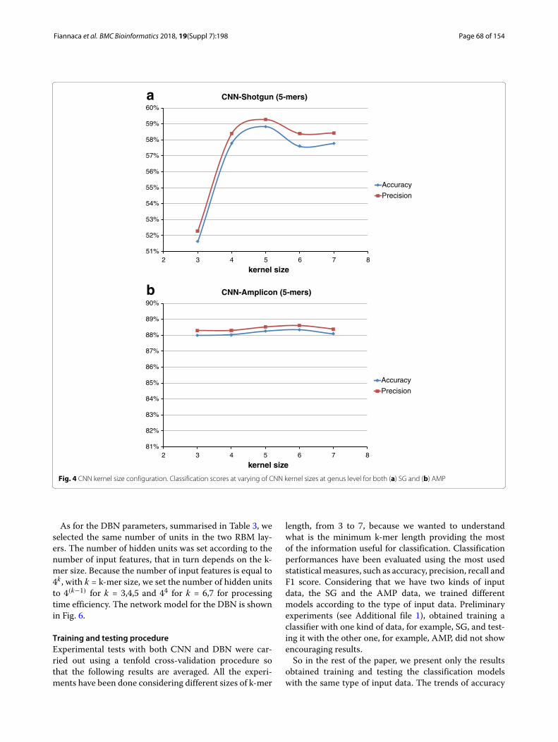
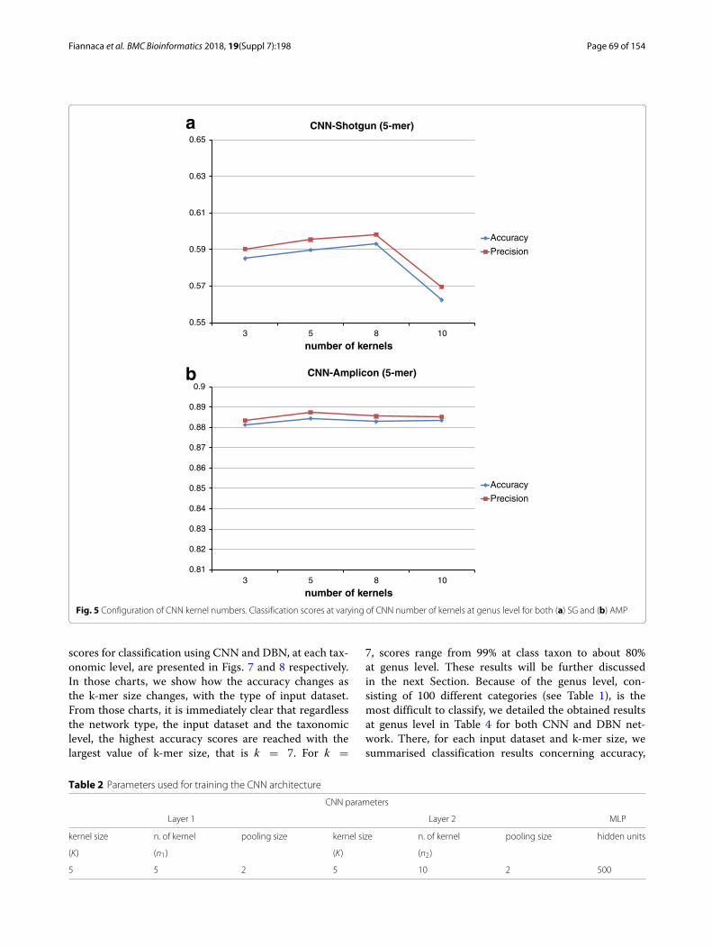
parameters, we performed a grid search to find a suit-able configuration that would represent a good trade-offbetween obtained results and processing time. In particu-lar, we noticed that classification results had a very slightlychange (less than 1%) on kernel size and the number ofkernels, as can be seen in Figs. 4 and 5 at the genus level.For this reason, we chose the CNN network configurationshown in Table 2.

Fig. 3 The convolutional neural network. The architecture of the convolutional neural network used. Here, L represents the dimension of the inputvector x, L = 4K were K is the dimension of the K-mers. In the upper part of the figure the representation of the C1 convolutional-maxpooling layer,where K stands for kernel size and n1 is the number of kernels. The blockM1 represents the set of weights for the connections from input to hiddenlayer, the blockM2 represents the weighted connections from hidden layer to output. y is the CNN output

Fiannaca et al. BMC Bioinformatics 2018, 19(Suppl 7):198 Page 68 of 154

81%

82%

83%

84%

85%

86%

87%

88%

89%

90%

2 3 4 5 6 7 8

kernel size

CNN-Amplicon (5-mers)

Accuracy

Precision

a

b

51%

52%

53%

54%

55%

56%

57%

58%

59%

60%

2 3 4 5 6 7 8

kernel size

CNN-Shotgun (5-mers)

Accuracy

Precision

Fig. 4 CNN kernel size configuration. Classification scores at varying of CNN kernel sizes at genus level for both (a) SG and (b) AMP

As for the DBN parameters, summarised in Table 3, weselected the same number of units in the two RBM lay-ers. The number of hidden units was set according to thenumber of input features, that in turn depends on the k-mer size. Because the number of input features is equal to4k , with k = k-mer size, we set the number of hidden unitsto 4(k−1) for k = 3,4,5 and 44 for k = 6,7 for processingtime efficiency. The network model for the DBN is shownin Fig. 6.

Training and testing procedureExperimental tests with both CNN and DBN were car-ried out using a tenfold cross-validation procedure sothat the following results are averaged. All the experi-ments have been done considering different sizes of k-mer

length, from 3 to 7, because we wanted to understandwhat is the minimum k-mer length providing the mostof the information useful for classification. Classificationperformances have been evaluated using the most usedstatistical measures, such as accuracy, precision, recall andF1 score. Considering that we have two kinds of inputdata, the SG and the AMP data, we trained differentmodels according to the type of input data. Preliminaryexperiments (see Additional file 1), obtained training aclassifier with one kind of data, for example, SG, and test-ing it with the other one, for example, AMP, did not showencouraging results.So in the rest of the paper, we present only the results

obtained training and testing the classification modelswith the same type of input data. The trends of accuracy

Fiannaca et al. BMC Bioinformatics 2018, 19(Suppl 7):198 Page 69 of 154

0.55

0.57

0.59

0.61

0.63

0.65

3 5 8 10

number of kernels

CNN-Shotgun (5-mer)

Accuracy

Precision

0.81

0.82

0.83

0.84

0.85

0.86

0.87

0.88

0.89

0.9

3 5 8 10

number of kernels

CNN-Amplicon (5-mer)

Accuracy

Precision

a

b

Fig. 5 Configuration of CNN kernel numbers. Classification scores at varying of CNN number of kernels at genus level for both (a) SG and (b) AMP

scores for classification using CNN and DBN, at each tax-onomic level, are presented in Figs. 7 and 8 respectively.In those charts, we show how the accuracy changes asthe k-mer size changes, with the type of input dataset.From those charts, it is immediately clear that regardlessthe network type, the input dataset and the taxonomiclevel, the highest accuracy scores are reached with thelargest value of k-mer size, that is k = 7. For k =

7, scores range from 99% at class taxon to about 80%at genus level. These results will be further discussedin the next Section. Because of the genus level, con-sisting of 100 different categories (see Table 1), is themost difficult to classify, we detailed the obtained resultsat genus level in Table 4 for both CNN and DBN net-work. There, for each input dataset and k-mer size, wesummarised classification results concerning accuracy,

Table 2 Parameters used for training the CNN architecture

CNN parameters

Layer 1 Layer 2 MLP

kernel size n. of kernel pooling size kernel size n. of kernel pooling size hidden units

(K) (n1) (K) (n2)

5 5 2 5 10 2 500

Fiannaca et al. BMC Bioinformatics 2018, 19(Suppl 7):198 Page 70 of 154

Table 3 Number of hidden units used for training the DBNarchitecture, at varying of k-mer size

DBN parameters

k-mer size RBM layer 1 hidden units RBM layer 2 hidden units

(k) (h1) (h2)

3 32 32

4 128 128

5 256 256

6 256 256

7 256 256

precision, recall and F1 score, considering mean valuesover the ten folds and the corresponding standard devi-ations. From those tables, we can notice that, as seen inthe previous charts, with k-mer size k = 7 we reached thebest scores, 91.3% of accuracy for AMP data and 85.5%of accuracy for SG data, with very similar values of pre-cision, recall and F1 score, and a standard deviation ofabout 0.01.

Comparison with RDP classifierOur classification approach of short reads of bacte-rial 16S rRNA has been compared uniquely with theRDP classifier [34] taking into consideration that itis the most adopted among the recent metagenomicspipelines, as highlighted in the Background Section. TheRDP classifier, version 2.5, has been trained and testedwith the same datasets we used in our experiments,considering a ten-fold cross-validation procedure andaveraging all the results. Comparisons of classificationperformances at the genus level, in terms of accuracy,

among the RDP classifier and our approaches with CNNand DBN, are presented in Fig. 9, using SG datasetand AMP dataset. From those charts, we can state thatour approach, with both CNN and DBN, reaches higherscores than RDP classifier, especially in the case of AMPdataset, where the gap is about 8 percentage points(83% vs. 91%).

Execution timesExperiments have been carried out on a cluster composedof 24 nodes with the following configuration:

• CPU: 1 X Intel(R) Xeon(R) CPU E5-2670 0 2.60GHz• RAM: 128 GBytes Memoria DDR3 1600 MHz• HD: 1TB SATA• GPU: 48 x GPU NVIDIA KEPLER K20• OS: Centos 6.3

Table 5 reports the average execution time in secondsfor a single fold. It shows obtained results for both trainingand testingmodels at varying of k value. Although trainingphase require several seconds, the testing phase is quitefast, even for k = 7.

DiscussionThe most interesting results we obtained is that thereare actual differences in classification performances onthe basis of the two type of input data analysed, SG orAMP. Considering the AMP dataset, in fact, all the clas-sifiers, CNN, DBN and RDP, reach their own best scores.This trend can be explained considering how the differentsequencing techniques, shotgun and amplicon, work. Asexplained in the Background Section, the reads producedwith the shotgun sequencing cover all the available

Fig. 6 The deep belief network. An example of deep belief network with two RBM layers for binary classification. In this figure, L represents thedimension of the input vector x, whereas, h and w represent the hidden units and the weights of each RBM respectively. y is the binary output

Fiannaca et al. BMC Bioinformatics 2018, 19(Suppl 7):198 Page 71 of 154

10%

20%

30%

40%

50%

60%

70%

80%

90%

100%

3 4 5 6 7

Acc

ura

cy

k-mer size

CNN-SG

Class

Order

Family

Genus

10%

20%

30%

40%

50%

60%

70%

80%

90%

100%

3 4 5 6 7

Acc

ura

cy

k-mer size

CNN-AMP

Class

Order

Family

Genus

a

b

Fig. 7 Accuracy validation of CNN classifier, according to k-mer size. Classification of (a) SG and (b) AMP datasets with CNN architecture

genome; whereas with the amplicon technique, only well-defined genomic regions are sequenced. In the case of16S rRNA, therefore, the SG dataset is composed of readsextracted from every part of the gene; the AMP dataset, inturn, is composed of reads belonging exactly to one hyper-variable region that, in our work is the V3-V4 region. Thatmeans the SG dataset is affected by noise in those readscovering the regions of 16S rRNA gene with little infor-mation content. On the other hand, the AMP dataset isvery focused, in a sense, it contains the most of the infor-mation content. The fact that a classifier trained on onedataset can’t be used with data of the other type indicatesthat the two datasets convey different information sets,even if the SG dataset seems a superset of the AMP. As

for the performance of the two deep learning approaches,we noticed that the key parameter is the size of thek-mer, because it is directly related to the size of inputrepresentation since the latter is equal to 4k . Especiallyfor CNN, in fact, from Fig. 7 it is clear the improvementof the accuracy score as the size of k-mer increases. Thistrend is more evident at the genus taxonomic level, wherethere are 100 different categories to classify. Moreover,looking at Fig. 7, from k-mer size = 5 to k-mer size = 6,the CNN approach has a noticeable boost of performance.The DBN approach, instead, has a more stable grow-ing trend (see Fig. 8). That means the generative modelinferred by the DBN can better estimate the statistic ofthe input data even for k-mer size below 5. In the case of

Fiannaca et al. BMC Bioinformatics 2018, 19(Suppl 7):198 Page 72 of 154

10%

20%

30%

40%

50%

60%

70%

80%

90%

100%

3 4 5 6 7

Acc

ura

cy

k-mer size

DBN-SG

Class

Order

Family

Genus

10%

20%

30%

40%

50%

60%

70%

80%

90%

100%

3 4 5 6 7

Acc

ura

cy

k-mer size

DBN-AMP

Class

Order

Family

Genus

a

b

Fig. 8 Accuracy validation of DBN classifier, according to k-mer size. Classification of (a) SG and (b) AMP datasets with DBN architecture

DBN, however, it is important to recall that also thenumber of hidden units depends on the value of k, becausewe set the number of hidden units to 4(k−1) for k =3,4,5 and 44 for k = 6,7. With regards to both compu-tational approaches, CNN and DBN, we noticed a verysimilar trend, above all for large value of k-mer size (6and 7). Considering, however, that the increase of per-formances between k=6 and k=7 is shrunk, we did notfurther investigated for larger value of k (i.e., 8 and 9),also taking into account the huge amount of neededprocessing time, with input vector of size 65536 and262144, respectively. Finally, considering the comparisonamong the classifiers, our approach based on CNN andDBN clearly overtakes the scores provided by the RDP

classifier. In particular, with regards to the AMP dataset,we reached an accuracy score at genus level of about91% with both networks against the 83% obtained withRDP. As for the SG dataset, our best result at genuslevel is about 85% with CNN, against 80% obtained withRDP.In this work, all the experiments have been carried

out using real 16S gene sequences, downloaded from theRDP database, from which simulated reads have beengenerated. We performed that approach in order to val-idate our classification pipeline but also because, at thebest of our knowledge, at present time there are not anyreal metagenomic datasets providing reads labelled witha taxonomic rank. Without that information, in fact, we

Fiannaca et al. BMC Bioinformatics 2018, 19(Suppl 7):198 Page 73 of 154

Table 4 Comparison among classification performances of CNN, DBN and RDP algorithms at varying of k-mer size. for both SG andAMP datasets

Evaluation of short-reads classification at genus level

Dataset Algorithm kAccuracy Precision Recall F1

mean % std mean % std mean % std mean % std

AMP

CNN

3 51.01 0.005 51.40 0.005 50.90 0.005 50.84 0.015

4 77.69 0.004 77.91 0.005 77.69 0.005 77.57 0.014

5 88.13 0.005 88.38 0.005 88.07 0.006 88.98 0.014

6 90.92 0.005 91.14 0.005 90.91 0.005 90.82 0.009

7 91.33 0.004 91.57 0.004 91.32 0.004 91.18 0.015

DBN

3 56.69 0.013 57.88 0.011 56.62 0.013 55.56 0.013

4 85.10 0.004 85.47 0.005 85.08 0.004 84.53 0.008

5 89.82 0.003 90.12 0.004 89.82 0.003 89.63 0.004

6 90.55 0.005 90.73 0.005 90.53 0.005 90.45 0.005

7 91.37 0.005 91.62 0.005 91.37 0.005 91.26 0.005

RDP - 83.84 0.007 84.42 0.007 83.57 0.007 83.65 0.007

SG

CNN

3 17.02 0.018 17.32 0.013 16.53 0.015 16.69 0.006

4 32.98 0.015 33.42 0.012 32.59 0.013 32.65 0.005

5 59.80 0.015 60.34 0.014 59.41 0.015 59.31 0.005

6 80.77 0.009 81.10 0.010 80.41 0.009 80.33 0.005

7 85.50 0.014 85.70 0.014 85.20 0.014 85.11 0.005

DBN

3 17.75 0.009 19.80 0.010 17.50 0.009 16.32 0.010

4 54.11 0.007 55.62 0.007 53.67 0.007 53.17 0.007

5 71.44 0.007 72.45 0.009 71.07 0.007 70.99 0.008

6 77.85 0.007 78.36 0.008 77.53 0.008 77.47 0.008

7 81.27 0.002 81.87 0.004 80.92 0.003 80.94 0.002

RDP - 80.38 0.009 80.83 0.008 80.18 0.008 80.09 0.009

are unable to measure the performances of our classifiersin terms of the main statistical scores introduced in theprevious Sections.

Implementation detailsBoth CNN and DBN models have been implementedas Python 2.7 scripts. As for CNN, we used the Keraslibrary (www.keras.io) with tensorflow backend; as forDBN,it has been implemented in Tensorflow, adaptingthe code available at https://github.com/albertbup/deep-belief-network. Source code and dataset are available athttps://github.com/IcarPA-TBlab/MetagenomicDC

ConclusionsIn this work, we proposed a 16S short-readsequences classification technique, for the analy-sis of metagenomic data. The proposed pipeline isbased on k-mer representation and deep learningarchitecture, and provide a classification model foreach taxa.

Experimental results confirmed the proposed pipelineas a valid approach for classifying bacteria sequencesfor both type of NGS technologies; for this reason, ourapproach could be integrated into the most common toolsfor metagenomic analysis. Also, we obtained a better clas-sification performance compared with the reference clas-sifier for microbiome analysis, i.e. the RDP classifier, forall considered taxa (until genus level). In detail, the per-centage of accuracy reached from our classifier, applied toAMP sequencing, has an increased score of about eightpercentage points at genus level with both CNN and DBN.Results showed that there are actual differences in classi-fication performances by the type of input data analysed,which are SG and AMP. In detail, the performance ofour classifier applied to AMP technology is, in average,better than SG. Further investigations will be conductedtrying to characterise the two kinds of networks, CNNsand DBNs, on special taxa or group of sequences, with thefinal goal of combining the two networks to improve thefinal classification of metagenome sequences.

Fiannaca et al. BMC Bioinformatics 2018, 19(Suppl 7):198 Page 74 of 154

70%

75%

80%

85%

90%

95%

Genus

Acc

ura

cy

CNN

DBN

RDP

70%

75%

80%

85%

90%

95%

Genus

Acc

ura

cy

CNN

DBN

RDP

a

b

Fig. 9 Accuracy validation of CNN, DBN and RDP classifiers, at genus level. Comparison among CNN, DBN and RDP classification algorithms, withrespect to (a) SG and (b) AMP datasets

Table 5 Average execution time in seconds for a single fold, obtained for both training and testing models at varying of k value.Although models training require several seconds, the testing phase is quite fast, even for k = 7

Execution times for training and testing models

kDBN CNN

Train (s) Test (s) Train (s) Test (s)

3 7288.913 0.111 686.403 0.240

4 8170.077 0.122 1256.652 0.375

5 11875.716 0.060 3091.721 0.719

6 20346.112 0.053 8021.737 1.506

7 37161.237 0.128 24204.754 3.986

Fiannaca et al. BMC Bioinformatics 2018, 19(Suppl 7):198 Page 75 of 154

Additional file

Additional file 1: Preliminary classification results. Preliminaryclassification results obtained training amodel with a kind of input data, e.g.SG, and testing it with the other type of input data, e.g. AMP. (XLSX 9.52 kb)

AbbreviationsAMP: Amplicon; CNN: Convolutional neural network; DBN: Deep beliefnetwork; MLP: Multilayer perceptron; NGS: Next Generation Sequencing; RBM:Restricted Boltzmann Machine; rRNA: ribosomal RNA; SG: Shotgun; WGS:Whole genome shotgun

FundingThe publication costs for this article were funded by the CNR InteromicsFlagship Project “- Development of an integrated platform for the applicationof “omic” sciences to biomarker definition and theranostic, predictive anddiagnostic profiles”.

Availability of data andmaterialsSource code and dataset are available at https://github.com/IcarPA-TBlab/MetagenomicDC

About this supplementThis article has been published as part of BMC Bioinformatics Volume 19Supplement 7, 2018: 12th and 13th International Meeting on ComputationalIntelligence Methods for Bioinformatics and Biostatistics (CIBB 2015/16). Thefull contents of the supplement are available online at https://bmcbioinformatics.biomedcentral.com/articles/supplements/volume-19-supplement-7.

Authors’ contributionsAF: project conception, system design, implementation, discussion, writing.LLP: project conception, system design, case studies, discussion, writing. MLR:project conception, system design, implementation, discussion, writing. GLB:project conception, system design, discussion, writing. GR: implementation,discussion. RR: project conception, system design, discussion, writing. SG:project conception, system design, discussion. AU: project conception, systemdesign, discussion, writing, funding. All authors read and approved the finalmanuscript.

Ethics approval and consent to participateNot applicable.

Competing interestsThe authors declare that they have no competing interests.

Publishers NoteSpringer Nature remains neutral with regard to jurisdictional claims inpublished maps and institutional affiliations.

Author details1CNR-ICAR, National Research Council of Italy, Via Ugo La Malfa, 153, Palermo,Italy . 2Dipartimento di Matematica e Informatica, Università degli studi diPalermo, Via Archirafi, 34, Palermo, Italy . 3Dipartimento dell’InnovazioneIndustriale e Digitale, Università degli studi di Palermo, Viale Delle Scienze,ed.6, Palermo, Italy .

Published: 9 July 2018

References1. Wooley JC, Ye Y. Metagenomics: Facts and Artifacts, and Computational

Challenges. J Comput Sci Technol. 2010;25(1):71–81.2. Rinke C, Schwientek P, Sczyrba A, Ivanova NN, Anderson IJ, Cheng JF, et

al. Insights into the phylogeny and coding potential of microbial darkmatter. Nature. 2013;499(7459):431–7.

3. Krebs C. Species Diversity Measures. In: Ecological Methodology. Boston:Addison-Wesley Educational; 2014. p. 531–95.

4. Simpson EH. Measurement of Diversity. Nature. 1949;163(4148):688–8.5. Escobar-Zepeda A, Vera-Ponce de León A, Sanchez-Flores A. The Road to

Metagenomics: From Microbiology to DNA Sequencing Technologiesand Bioinformatics. Front Genet. 2015;6(348).

6. Simon C, Daniel R. Metagenomic analyses: past and future trends. ApplEnviron Microbiol. 2011;77(4):1153–61.

7. Raes J, Letunic I, Yamada T, Jensen LJ, Bork P. Toward moleculartrait-based ecology through integration of biogeochemical, geographicaland metagenomic data. Mol Syst Biol. 2014;7(1):473.

8. Qin J, Li Y, Cai Z, Li S, Zhu J, Zhang F, et al. A metagenome-wideassociation study of gut microbiota in type 2 diabetes. Nature.2012;490(7418):55–60.

9. Turnbaugh PJ, Ley RE, Mahowald MA, Magrini V, Mardis ER, Gordon JI.An obesity-associated gut microbiome with increased capacity forenergy harvest. Nature. 2006;444(7122):1027–31.

10. Turnbaugh PJ, Hamady M, Yatsunenko T, Cantarel BL, Duncan A, LeyRE, et al. A core gut microbiome in obese and lean twins. Nature.2009;457(7228):480–4.

11. Karlsson FH, Fåk F, Nookaew I, Tremaroli V, Fagerberg B, Petranovic D,et al. Symptomatic atherosclerosis is associated with an altered gutmetagenome. Nat Commun. 2012;3:1245.

12. Karlsson FH, Tremaroli V, Nookaew I, Bergström G, Behre CJ, FagerbergB, et al. Gut metagenome in European women with normal, impaired anddiabetic glucose control. Nature. 2013;498(7452):99–103.

13. Tringe SG, Hugenholtz P. A renaissance for the pioneering 16S rRNAgene. Curr Opin Microbiol. 2008;11(5):442–6.

14. Wang Y, Qian PY. Conservative Fragments in Bacterial 16S rRNA Genesand Primer Design for 16S Ribosomal DNA Amplicons in MetagenomicStudies. PLoS ONE. 2009;4(10):e7401.

15. Yang B, Wang Y, Qian PY. Sensitivity and correlation of hypervariableregions in 16S rRNA genes in phylogenetic analysis. BMC Bioinformatics.2016;17(1):135.

16. Kalyuzhnaya MG, Lapidus A, Ivanova N, Copeland AC, McHardy AC,Szeto E, et al. High-resolution metagenomics targets specific functionaltypes in complexmicrobial communities. Nat Biotechnol. 2008;26(9):1029–34.

17. Salipante SJ, Kawashima T, Rosenthal C, Hoogestraat DR, Cummings LA,Sengupta DJ, et al. Performance Comparison of Illumina and Ion TorrentNext-Generation Sequencing Platforms for 16S rRNA-Based BacterialCommunity Profiling. Appl Environ Microbiol. 2014;80(24):7583–91.

18. Quail M, Smith ME, Coupland P, Otto TD, Harris SR, Connor TR, et al. Atale of three next generation sequencing platforms: comparison of Iontorrent, pacific biosciences and illumina MiSeq sequencers. BMCGenomics. 2012;13(1):341.

19. Huttenhower C, Gevers D, Knight R, Abubucker S, Badger JH, ChinwallaAT, et al. Structure, function and diversity of the healthy humanmicrobiome. Nature. 2012;486(7402):207–14.

20. Soergel DA, Dey N, Knight R, Brenner SE. Selection of primers for optimaltaxonomic classification of environmental 16S rRNA gene sequences.ISME J. 2012;6(7):1440–4.

21. D’Amore R, Ijaz UZ, Schirmer M, Kenny JG, Gregory R, Darby AC, et al. Acomprehensive benchmarking study of protocols and sequencingplatforms for 16S rRNA community profiling. BMC genomics. 2016;17(1):55.

22. Zheng W, Tsompana M, Ruscitto A, Sharma A, Genco R, Sun Y, et al. Anaccurate and efficient experimental approach for characterization of thecomplex oral microbiota. Microbiome. 2015;3(1):48.

23. Chakravorty S, Helb D, Burday M, Connell N, Alland D. A detailedanalysis of 16S ribosomal RNA gene segments for the diagnosis ofpathogenic bacteria. J Microbiol Methods. 2007;69(2):330–9.

24. Hayssam S, Macha N. Machine learning for metagenomics: methods andtools. Metagenomics. 2016;1:1–19.

25. Huson DH, Auch AF, Qi J, Schuster SC. MEGAN analysis of metagenomicdata. Genome Res. 2007;17(3):377–86.

26. Kultima JR, Sunagawa S, Li J, Chen W, Chen H, Mende DR, et al. MOCAT:A Metagenomics Assembly and Gene Prediction Toolkit. Plos ONE.2012;7(10):e4765.

27. Miller CS, Baker BJ, Thomas BC, Singer SW, Banfield JF. EMIRGE:reconstruction of full-length ribosomal genes from microbial communityshort read sequencing data. Genome Biol. 2011;12(5):R44.

28. Shah N, Tang H, Doak TG, Ye Y. Comparing Bacterial CommunitiesInferred from 16s Rrna Gene Sequencing and Shotgun Metagenomics. In:Pacific Symposium on Biocomputing Pacific Symposium onBiocomputing. Singapore: World Scientific; 2011. p. 165–76.

29. Yuan C, Lei J, Cole J, Sun Y. Reconstructing 16S rRNA genes inmetagenomic data. Bioinformatics. 2015;31(12):i35.

30. Albanese D, Fontana P, De Filippo C, Cavalieri D, Donati C. MICCA: acomplete and accurate software for taxonomic profiling of metagenomicdata. Sci Rep. 2015;5:9743.

Fiannaca et al. BMC Bioinformatics 2018, 19(Suppl 7):198 Page 76 of 154

31. Ramazzotti M, Berná L, Donati C, Cavalieri D. riboFrame: An ImprovedMethod for Microbial Taxonomy Profiling from Non-TargetedMetagenomics. Front Genet. 2015;6:329.

32. Nawrocki EP, Kolbe DL, Eddy SR. Infernal 1.0: inference of RNAalignments. Bioinformatics. 2009;25(10):1335.

33. Chaudhary N, Sharma AK, Agarwal P, Gupta A, Sharma VK. 16S Classifier:A Tool for Fast and Accurate Taxonomic Classification of 16S rRNAHypervariable Regions in Metagenomic Datasets. PLoS ONE. 2015;10(2):e0116106.

34. Wang Q, Garrity GM, Tiedje JM, Cole JR. Naive Bayesian classifier for rapidassignment of rRNA sequences into the new bacterial taxonomy. ApplEnviron Microbiol. 2007;73(16):5261–7.

35. LeCun Y, Bengio Y, Hinton G. Deep learning. Nature. 2015;521:436–44.36. Lo Bosco G, Rizzo R, Fiannaca A, La Rosa M, Urso A. A Deep Learning

Model for Epigenomic Studies. In: 2016 12th International Conference onSignal-Image Technology Internet-Based Systems (SITIS). New York: IEEE;2016. p. 688–92.

37. Lo Bosco G, Di Gangi MA. In: Petrosino A, Loia V, Pedrycz W, editors.Deep Learning Architectures for DNA Sequence Classification. Cham:Springer International Publishing; 2017, pp. 162–71.

38. Di Gangi MA, Gaglio S, La Bua C, Lo Bosco G, Rizzo R. In: Rojas I, OrtuñoF, editors. A Deep Learning Network for Exploiting Positional Informationin Nucleosome Related Sequences. Cham: Springer InternationalPublishing; 2017, pp. 524–33.

39. Min S, Lee B, Yoon S. Deep learning in bioinformatics. Brief Bioinform.2017;18(5):851–69.

40. Angly FE, Willner D, Rohwer F, Hugenholtz P, Tyson GW. Grinder: aversatile amplicon and shotgun sequence simulator. Nucleic Acids Res.2012;40(12):e94.

41. Park Y, Kellis M. Deep learning for regulatory genomics. Nat Biotechnol.2015;33(8):825–6.

42. Alipanahi B, Delong A, Weirauch MT, Frey BJ. Predicting the sequencespecificities of DNA-and RNA-binding proteins by deep learning. NatBiotechnol. 2015;33(8):831–8.

43. Zeng H, Edwards MD, Liu G, Gifford DK. Convolutional neural networkarchitectures for predicting DNA–protein binding. Bioinformatics.2016;32(12):i121–7.

44. Fiannaca A, La Rosa M, Rizzo R, Urso A. Analysis of DNA BarcodeSequences Using Neural Gas and Spectral Representation. In: Iliadis L,Papadopoulos H, Jayne C, editors. Engineering Applications of NeuralNetworks. vol. 384 of Communications in Computer and InformationScience. Berlin, Heidelberg: Springer; 2013. p. 212–221.

45. Fiannaca A, La Rosa M, Rizzo R, Urso A. A k-mer-based barcode DNAclassification methodology based on spectral representation and a neuralgas network. Artif Intell Med. 2015;64(3):173–84.

46. Pinello L, Lo Bosco G, Hanlon B, Yuan GC. A motif-independent metricfor DNA sequence specificity. BMC Bioinformatics. 2011;12:1–9.

47. Soueidan H, Nikolski M. Machine learning for metagenomics: methodsand tools. Metagenomics. 2016;1:1–19.

48. Chor B, Horn D, Goldman N, Levy Y, Massingham T. Genomic DNAk-mer spectra: models and modalities. Genome Biol. 2009;10(10):R108.

49. Kuksa P, Pavlovic V. Efficient alignment-free DNA barcode analytics. BMCBioinformatics. 2009;10(14):S9.

50. Vilo C, Dong Q. Evaluation of the RDP Classifier Accuracy Using 16S rRNAGene Variable Regions. Metagenomics. 2012;1:1–5.

51. Hinton GE. Reducing the dimensionality of data with neural networks.Science. 2006;313(5786):504–7.

52. LeCun Y, Bottou L, Bengio Y, Haffner P. Gradient-based learning appliedto document recognition. Proc IEEE. 1998;86(11):2278–324.

53. Hinton GE, Osindero S, Teh YW. A fast learning algorithm for deep beliefnets. Neural Comput. 2006;18(7):1527–54.

54. Hinton GE. Training products of experts by minimizing contrastivedivergence. Neural Comput. 2002;14(8):1771–800.

55. Kullback S, Leibler RA. On Information and Sufficiency. Ann Math Stat.1951;22(1):79–86.

56. Walker SH, Duncan DB. Estimation of the probability of an event as afunction of several independent variables. Biometrika. 1967;54(1/2):167–79.

57. Rizzo R, Fiannaca A, La Rosa M, Urso A. A Deep Learning Approach toDNA Sequence Classification. In: Computational Intelligence Methods forBioinformatics and Biostatistics. vol. 9874 of Lecture Notes in ComputerScience; 2016. p. 129–40.