
Research Article Modeling, Parameters...
11
Research Article Modeling, Parameters Identification, and Control of High Pressure Fuel Cell Back-Pressure Valve Fengxiang Chen, Ling Liu, Shiguang Liu, and Tong Zhang Clean Energy Automotive Engineering Center, Tongji University, Shanghai 201804, China Correspondence should be addressed to Fengxiang Chen; [email protected] Received 5 June 2014; Revised 5 September 2014; Accepted 19 September 2014; Published 16 November 2014 Academic Editor: Yan Liang Copyright © 2014 Fengxiang Chen et al. is is an open access article distributed under the Creative Commons Attribution License, which permits unrestricted use, distribution, and reproduction in any medium, provided the original work is properly cited. e reactant pressure is crucial to the efficiency and lifespan of a high pressure PEMFC engine. is paper analyses a regulated back- pressure valve (BPV) for the cathode outlet flow in a high pressure PEMFC engine, which can achieve precisely pressure control. e modeling, parameters identification, and nonlinear controller design of a BPV system are considered. e identified parameters are used in designing active disturbance rejection controller (ADRC). Simulations and extensive experiments are conducted with the xPC Target and show that the proposed controller can not only achieve good dynamic and static performance but also have strong robustness against parameters’ disturbance and external disturbance. 1. Introduction High pressure proton exchange membrane fuel cell (PEMFC) engines offer clean and efficient energy production and are advantaged of high stack power density, quick system response, and easy humidification. One of the dominant design parameters for high pressure PEMFC system is the operating pressure [1]. In the case of stored compressed hydrogen, the pressure of the cathode air supply system becomes an important optimized parameter [2]. Com- pared with the low-pressure system, high operating pressure improves the performance of the fuel cell stack but consumes more power due to the flow device, such as the compressor (nearly consuming up to 20 percent of the net power [3]). In order to maintain a high efficiency during operation, it is important to control air pressure effectively. In this study, an electronic throttle (ET) body is served as a back-pressure valve (BPV); the cathode air supply system can operate in a proper pressure mainly by auto-tuning the angle of the BPV for cathode outlet flow at a given power. erefore, the fast and accurate control of the angle of the BPV is a key issue to regulate the back pressure for a high pressure PEMFC engine. e analysis of BPV model-based control system may begin with the mathematical model of a BPV system. e BPV is different from the traditional ET in that it has to consider the influence of the flow resistance. In addition, the BPV has many unknown parameters and there is no systematic method to estimate its parameters so far. Song has estimated some parameters [4]. e simulations show that the model and real plant have unacceptable bias due to excess approximation. Grep and Lee have designed some simple algorithms [5] and modified them to identify the ET parameters in [6]. But there is no mention of the parameter verification. Based on the previous studies, several algorithms are developed to estimate the unknown parameters in this paper. Parameter identification uses simple equipment, such as current, voltage sensor, and obtained parameters are optimized through the optimization toolbox. e model and acquired parameters can be used for the model-based con- troller design. What is more, they can also be used to find out the optimal opening of the BPV at a given power by merging into a PEMFC model. At present, set-points are usually obtained by repeating experiments on PEMFC engine. In the aspect of control, various control design techniques have been studied in the previous publications, such as proportional-integral-derivative (PID) control [7] and sliding mode control [8]. In [9], the application of receptive field weighted regression (RFWR) method is demonstrated for the composite control of ET. In [10], an ET controller based on the idea of back-stepping method is proposed, which meets Hindawi Publishing Corporation Mathematical Problems in Engineering Volume 2014, Article ID 246015, 10 pages http://dx.doi.org/10.1155/2014/246015
Transcript of Research Article Modeling, Parameters...
Research ArticleModeling Parameters Identification and Control ofHigh Pressure Fuel Cell Back-Pressure Valve
Fengxiang Chen Ling Liu Shiguang Liu and Tong Zhang
Clean Energy Automotive Engineering Center Tongji University Shanghai 201804 China
Correspondence should be addressed to Fengxiang Chen fxchentongjieducn
Received 5 June 2014 Revised 5 September 2014 Accepted 19 September 2014 Published 16 November 2014
Academic Editor Yan Liang
Copyright copy 2014 Fengxiang Chen et alThis is an open access article distributed under theCreativeCommonsAttribution Licensewhich permits unrestricted use distribution and reproduction in any medium provided the original work is properly cited
The reactant pressure is crucial to the efficiency and lifespan of a high pressure PEMFC engineThis paper analyses a regulated back-pressure valve (BPV) for the cathode outlet flow in a high pressure PEMFC engine which can achieve precisely pressure controlThemodeling parameters identification and nonlinear controller design of a BPV system are consideredThe identified parametersare used in designing active disturbance rejection controller (ADRC) Simulations and extensive experiments are conducted withthe xPC Target and show that the proposed controller can not only achieve good dynamic and static performance but also havestrong robustness against parametersrsquo disturbance and external disturbance
1 Introduction
High pressure proton exchangemembrane fuel cell (PEMFC)engines offer clean and efficient energy production andare advantaged of high stack power density quick systemresponse and easy humidification One of the dominantdesign parameters for high pressure PEMFC system is theoperating pressure [1] In the case of stored compressedhydrogen the pressure of the cathode air supply systembecomes an important optimized parameter [2] Com-pared with the low-pressure system high operating pressureimproves the performance of the fuel cell stack but consumesmore power due to the flow device such as the compressor(nearly consuming up to 20 percent of the net power [3])In order to maintain a high efficiency during operation itis important to control air pressure effectively In this studyan electronic throttle (ET) body is served as a back-pressurevalve (BPV) the cathode air supply system can operate in aproper pressure mainly by auto-tuning the angle of the BPVfor cathode outlet flow at a given power Therefore the fastand accurate control of the angle of the BPV is a key issue toregulate the back pressure for a high pressure PEMFC engine
The analysis of BPV model-based control system maybegin with the mathematical model of a BPV system TheBPV is different from the traditional ET in that it has to
consider the influence of the flow resistance In additionthe BPV has many unknown parameters and there is nosystematic method to estimate its parameters so far Songhas estimated some parameters [4] The simulations showthat the model and real plant have unacceptable bias dueto excess approximation Grep and Lee have designed somesimple algorithms [5] and modified them to identify the ETparameters in [6] But there is no mention of the parameterverification Based on the previous studies several algorithmsare developed to estimate the unknown parameters in thispaper Parameter identification uses simple equipment suchas current voltage sensor and obtained parameters areoptimized through the optimization toolbox The model andacquired parameters can be used for the model-based con-troller designWhat is more they can also be used to find outthe optimal opening of the BPV at a given power by merginginto a PEMFC model At present set-points are usuallyobtained by repeating experiments on PEMFC engine
In the aspect of control various control design techniqueshave been studied in the previous publications such asproportional-integral-derivative (PID) control [7] and slidingmode control [8] In [9] the application of receptive fieldweighted regression (RFWR)method is demonstrated for thecomposite control of ET In [10] an ET controller based onthe idea of back-stepping method is proposed which meets
Hindawi Publishing CorporationMathematical Problems in EngineeringVolume 2014 Article ID 246015 10 pageshttpdxdoiorg1011552014246015
2 Mathematical Problems in Engineering
the general requirements of the state stability Then in [11]the back-stepping controller combined with state observeris designed for the real-time system In [12] a variablestructure concept is utilized based on the sliding modeobserver technique and feedback back-stepping techniqueHowever the above methods have strongmodel dependenceParameters-varying or external disturbances can usuallydeteriorate the control performance Most importantly thesystem parameters used in the simulations are not verifiedwith actual ET model
In this paper a detailed nonlinear dynamic model ofBPV is provided and several algorithms are designed toestimate the unknown parameters The methods used inthe identification process consist of extensive measurementsexperiments and verifications The back-pressure valve usedin this paper is a commercial available ET system made byBosch in type of DV-E5 The rest of the paper is organizedas follows in Section 2 a detailed nonlinear dynamic modelof BPV is provided Next in Section 3 the identification algo-rithms are explained Finally the active disturbance rejectioncontroller (ADRC) is designed based on the mathematicalmodel and the identified parameters in Section 4 After thatthe model controlling effect and real-time controlling effectare presented
2 Modeling of the Back-Pressure Valve
The ET is featured with high nonlinearity The model of EThas been approached which includes the nonlinear returnspring and friction model Yet the BPV model is differentfrom the traditional ET in that it has to consider the influenceof the flow resistance
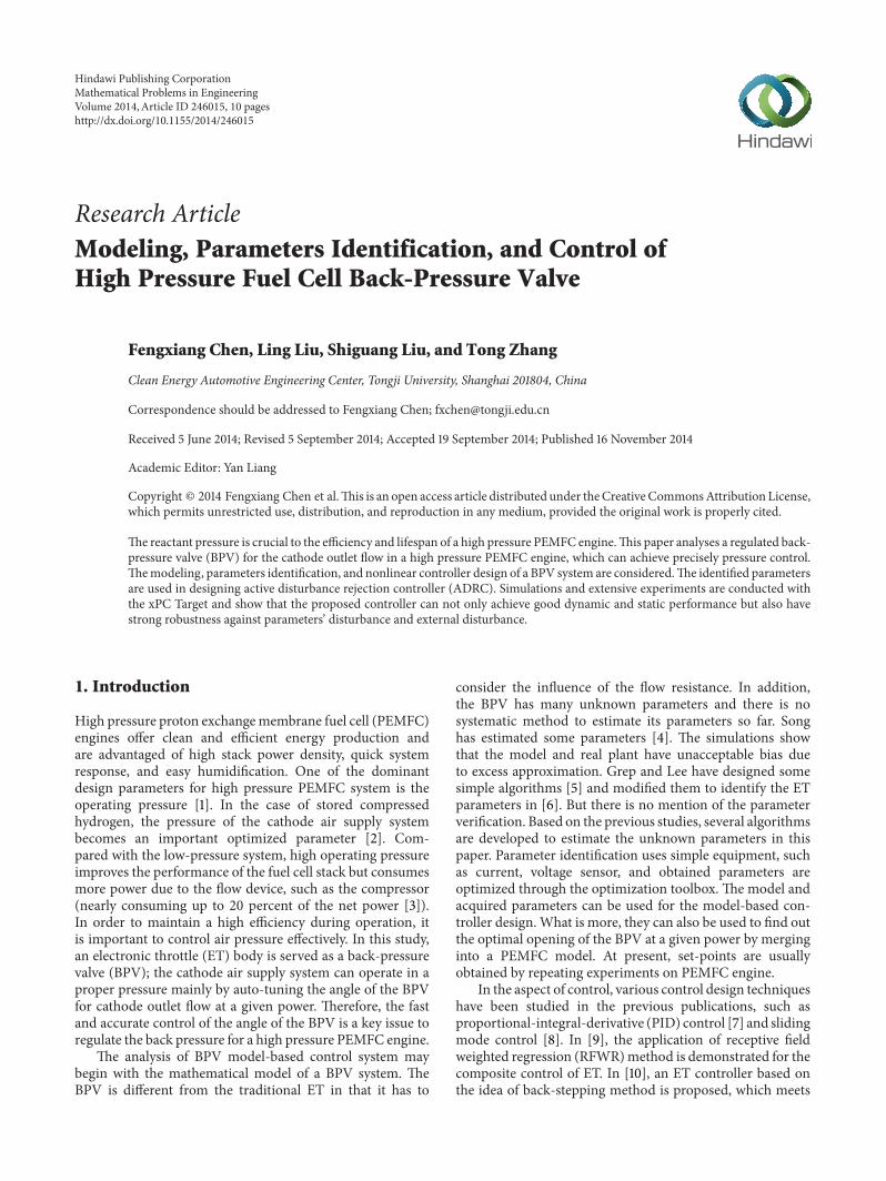
The BPV is a variable flow resistance device whichprovides needed pressure based on the position of the valveplate It consists of a brushed DC motor with permanentmagnets linked to the valve shaft by means of a set of spurgearbox a nonlinear return spring system a valve plate andtwo redundant potentiometers (Figure 1) [13]
21 MechanismModeling Themotor voltage 119864119886is defined as
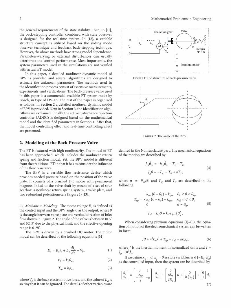
the control input and the BPV angle 120579 as the output where 120579is the angle between valve plate and vertical direction of inletflow shown in Figure 2The angle of the valve is between 105∘and 1015∘ due to the physical limit and the effective openingrange is 0ndash91∘
The BPV is driven by a brushed DC motor The motormodel can be described by the following equations [14]
119864119886= 119877119886119894119886+ 119871119886
119889119894119886
119889119905+ 119881119887 (1)
119881119887= 119896119887
120579119898 (2)
119879119898= 119896119905119894119886 (3)
where119881119887is the back electromotive force and the value of119871
119886is
so tiny that it can be ignoredThe details of other variables are
120579m
120579 Returnspring
Position sensor
Reduction gear Valve
Ea
Ra LaM
Figure 1 The structure of back-pressure valve
120579
Figure 2 The angle of the BPV
defined in the Nomenclature part The mechanical equationsof the motion are described by
119869119898
120579119898= minus119896119898
120579119898minus 119879119871+ 119879119898
119869119892
120579 = minus119879sp minus 119879tf + 119899119879119871(4)
where 119899 = 120579119898120579 and 119879sp and 119879tf are described in the
following
119879sp =
119896op (120579 minus 1205790) + 119896pre 1205790lt 120579 lt 120579op
119896cl (120579 minus 1205790) minus 119896pre 120579cl lt 120579 lt 12057900 120579 = 120579
0
119879tf = 119896119891120579 + 119896tf sgn ( 120579)
(5)
When considering previous equations (1)ndash(5) the equa-tion ofmotion of the electromechanical system can bewrittenin form
119869 120579 + 1198992
119896119898
120579 + 119879sp + 119879tf = 119899119896119905119894119886 (6)
where 119869 is the inertial moment in normalized units and 119869 =119869119892+ 1198992
119869119898
If we define1199091= 120579119909
2= 120579 as state variables 119906 isin [minus119864
119886 119864119886]
as the controlled input then the system can be described by
[1
2
] = [
[
0 1
minus
119896sp
119869minus119886
]
]
[1199091
1199092
] + [
[
0
119899119896119905
119869119877119886
]
]
119906 + [0
119887 (1199092)] + [
0
1] 119889
(7)
Mathematical Problems in Engineering 3
where 119887(1199092) = (minus119896tf sgn(1199092)+119896sp1205790 minus119896pre sgn(1199091 minus1205790))119869 119886 =
(1198992
119896119898+ 119896119891+ 1198992
119896119887119896119905119877119886)119869 and 119889 stands for the summation
of unmodeled dynamics and unknown disturbances forexample the load torque of inlet flow
22 Fluid Modeling This model is based on the PEMFCmodel proposed by Pukrushpan [15] The mass conservationprinciple is used to develop the outlet manifold model Forany manifold
119889119898
119889119905= 119882in minus119882out (8)
where 119882in and 119882out are mass flow rates in and out of themanifold respectively
The temperature of the stack has been well regulated to aconstant by the thermal management of the PEMFC There-fore the change of air temperature in the outlet manifold isnegligible and thus the pressure can be determined by
119889119901om119889119905
=
119877119892119879om
119881om
119889119898
119889119905 (9)
The outlet mass flow is governed by a BPV The BPVis a variable flow resistance device which provides neededpressure based on the position of the valve plate The flow isa function of manifold pressure 119901om the valve angle 120579 thediameter of the BPV 119863 and the downstream pressure of themanifold 119901atm Thus the air flow through the BPV satisfies[16]
119876119873= 285119860119870
11988101198632radic1199012Δ119901
119878 (10)
1198701198810=1 minus cos 120579radic119890cos
2120579
(11)
Δ119901 =
1199011minus 1199012
1199012
1199012
gt 05
1199012
1199012
1199012
le 05
(12)
where 1198701198810
is the flow coefficient which is related to theopening of the BPV and 0 le 119870
1198810le 1119863 is the valve diameter
119860 is the structure constant which can be set to 62 for ourBPV [16] Δ119901 (kgfcm2) is the pressure drop after the valve(which is less than half of the inlet pressure) 119901
1= 119901om
1199012= 119901atmWhen the pressure drop exceeds the limit the flow
dynamic will be choked which may lead to the instability ofthe flow rate [17] Choked phenomenon is shown in Figure 3where Δ119901cr is the critical pressure When pressure differenceexceeds the critical pressure for example Δ119901 = Δ119901
119886 the
actual flow is 119876max where 1198761015840
max ≫ 119876max
3 Parameter Identification
The valve parameters are usually unknown or cannot beaccurately measured Advanced nonlinear control algorithmrequires modeling of the plant and good estimate of itsparametersThis section provides some techniques to identifythe parameters of the aforementioned model [18]
radicΔparadicΔp
Q
Qmax
radicΔpcr
Q998400max
Figure 3 Choked phenomenon
Monitor Plant
DAQ cardTarget computer
Host computer
Figure 4 xPC Target platform
31 xPC Target The real-time simulation of rapid controlprototyping (RCP) is that the real plant is controlled bysimulating model For our RCP we have used xPC Targetsystem (Figure 4) Various tests are conducted to estimate theparameters on the platform
32 Characteristic Curve The plant has two potentiometerssupplied by 5-volt DC The calibration curves of ThrottlePosition Sensor (TPS) 1 and TPS2 are shown in Figure 5The angle of the valve is between 105∘ and 1015∘ due to thephysical limit When there is no voltage applied to the drivenmotor the output voltage of TPS1 is 083V so the defaultposition 120579
0is 175∘
33 Identification of 119877119886 There is nearly no rotation when a
slowly changing voltage is applied to the motor at the almostclosed position [19] Since the motor current changes slowlythe voltage across the inductance can be neglected Besidesthe inner resistance of the storage can be ignored Thereforethe armature circuit equations (1) and (2) can be described by
119864119886= 119877119886119894119886 (13)
Figure 6 displays the captured curves of themotor voltageagainst the motor current Due to the good symmetry ofthe H-bridge the direction of the current and voltage is
4 Mathematical Problems in Engineering
105 1015 105
5485
Volta
ge (V
)
05
Potentiometer track angel (∘)
Lead potentiometer
Gradient plusmn 00476
TPS 1TPS 2
Figure 5 Characteristic curve of angle sensors
Curr
ent (
A)
Voltage (V)
MeasuredApproximated
1
05
005 1 15
15
2 25
Figure 6 Motor current versus voltage
neglected The inverse of the slope represents the armatureresistance which reads 119877
119886= 20Ω
34 Identification of 119896119887 The circuit equations (1) and (2) can
be rewritten as
119881119887= 119899119896119887
120579 = 119864119886minus 119877119886119894119886 (14)
where 119899 = 2068 is the total gear ratio of the two set reductiongearThe back-EMF voltage is generated when the valve shaftis rotating Figure 7 shows the captured back-EMF voltageand the platersquos angular velocity
We get the back electromotive force constant 119896119887
=
00184V(rads) at the time when the platersquos angular velocityis steady Usually 119896
119887and 119896119905are almost the same for onemotor
35 Static Load Test Figure 8 shows the typical systemresponse when inputting sinusoidal signal If the frequency
2
1
0
minus1
minus2
minus3
minus4
minus51211510510 1195985
Angle (rad)
Back-EMF voltage (V)
Angular velocity (rads)
Time (s)
Figure 7 Velocity versus back-EMF voltage
10 20 30 40 50 60 70 80
0
5
10 20 30 40 50 60 70 80
0
2
4
10 20 30 40 50 60 70 800
1
2
minus5
minus2
minus4
Inpu
t vol
tage
(V)
Curr
ent (
A)
Ang
ular
(rad
)
Time (s)
Figure 8 Static loads test
is low the angular velocity and angular acceleration can beignored Therefore the dynamic equation of the system canbe described by
119896sp (120579 minus 1205790) + 119896pre sgn (120579 minus 1205790) + 119896tf sgn 120579 = 119899119896119905119894119886= 119879 (15)
The response plotted in load torque versus angle charac-teristic is shown in Figure 9 This experiment identifies theparameters 119896sp 119896pre and 119896tf
(1) The inverse slope of the inserted straight lines rep-resented the spring stiffness which reads 119896op =
04387N sdotmrad 119896cl = 73693N sdotmrad(2) The friction torque is half of the deviation between
two inserted straight lines during the opening time orthe closing time 119896tf = 02565N sdotm
(3) The preload torque applied to the valve at the defaultposition is 03829N sdotm
36 Viscous Coefficient Identification In this experiment wetake off the middle gear then the motor is separated from
Mathematical Problems in Engineering 5
18
16
14
12
1
08
06
04
02
0minus15 minus1 minus05 0 05 1 15
Ang
le (r
ad)
Load torque (Nm)
Figure 9 Plate angle versus load torque
16
15
14
13
12
11
1
05 1 15 2 25 3 35 4 45 5
times10minus4
Ea minus Ra lowast ia
ApproximatedMeasured
ktlowastkblowasti a
Figure 10 Data fit curve
the rest of the assembly When a DC voltage is applied to themotor the motor can run freely which is given by
119864119886= 119877119886119894119886+ 119896119887
120579119898
119869119898
120579119898= 119896119905119894119886minus 119896119898
120579119898
(16)
When the motor reaches steady velocity (16) can bewritten in form
119864119886minus 119877119886119894119886
119896119905119894119886
=119896119887
119896119898
(17)
Motor voltage along with the armature current is plottedusing Matlab cftool shown in Figure 10
The slope of the line gives the spring constant which reads119896119898= 15times10
minus5NsdotmradsThe viscous coefficient of the plateis small and can be ignored in this section We will identify itin the optimization section
11 12 13 14 15 16
0
2
4
6
8
minus2
minus4
minus6
minus8
minus10
Load torque (Nm)
Angular acceleration (rads2)
t (s)
Figure 11 Angular acceleration versus load torque
Table 1 Parameters value
Parameters Identified valueInitial Optimized
119869 (kgsdotm2) 00225 000297119896119887(Vsdotsrad) 00184 001681
119896cl (Nmrad) 73653 36221119896119891(Nmsdotsrad) mdash 000134
119896119898(Nmsdotsrad) 15119890 minus 05 142130119890 minus 05
119896op (Nmrad) 04387 021249119896pre (Nm) 03829 05306119896119905(NmsdotAminus1) 00184 002505
119896tf (Nm) 02565 037039119877119886(Ω) 2 19306
1205790(rad) 03053 0302
119899 2068 2068
37 Moment of Inertia Identification When 120579 gt 0 and 120579 gt 1205790
the system can be simplified to
119869 120579 + (1198992
119896119898+ 119896119891) 120579 + 119896tf + 119896sp (120579 minus 1205790) + 119896pre = 119899119896119905119894119886 (18)
Figure 11 shows the captured load torque and angularacceleration calculated by taking derivative of angular veloc-ity and angular velocity is the derivative of the position Themoment of inertia at the steady time of 138 s is 00225 kg sdotm2
38 Optimization Simulink Design Optimization is a tool-box provided by Matlab which can estimate the unknownparameters in a model Due to the approximation of theprevious experiments there are some errors to the modelparametersTherefore we optimized the previous parametersusing parameter estimate tool In the process of optimizationthe initial values are set to the values identified above and therange for each parameter is defined The algorithm used onoptimization is nonlinear least squaremethodTheoptimizedparameters are listed in Table 1
39 Parameters Verification In this section we will com-pare the simulation results with the real measurement
6 Mathematical Problems in Engineering
2 4 6 8 10 12 1410
20
30
40
50
60
70
80
90
100
Time (s)
Ang
le (∘
)
Angle simAngle measured
(a) Subjected to sinusoidal input
1 2 3 4 510
20
30
40
50
60
70
80
90
100
110
Time (s)
Ang
le (∘
)
Angle simAngle measured
05 15 25 35 45
(b) Subjected to a step input
Figure 12 Parameters verification subjected to sinusoidal and step input
Figure 12 shows the response of the real system versus modelwhen subjected to different control inputs Obviously thesimulations give a good fit to the real outputs
4 Controller Design
As mentioned above the BPV system is featured with strongnonlinearity and two order dynamics Thus the simpleapplication of standard PID controller may not work veryeffectively ADRC is a new control algorithm based on theactive disturbance rejection concept which can cope withthe highly nonlinear dynamics With ADRC the unknowndynamics and disturbances can be actively estimated andcompensated and it makes the feedback controller morerobust In fact systemrsquos equation (7) can be abstracted asthe following second-order nonlinear system with externaldisturbances
1= 1199092
2= 119891 (119909
1 1199092 119905) + 119908 (119905) + 119887
0119906
119910 = 1199091
(19)
where 1199091 1199092are system states 119891 is a smooth function 119908(119905)
is the external disturbance 1198870is the system parameter and 119906
is the control input signal The key of ADRC is to design anextended state observer (ESO) to estimate not only states butalso the ldquototal disturbancerdquo which contains internal uncertaindynamics and external disturbance
ADRC consists of three parts transient profile generatornonlinear state error feedback control law and extended stateobserver Taking second-order controlled object for examplethe structure of active disturbance rejection controller isshown in Figure 13 [20]
41 Transient Profile Generator Reasonable arrangement ofthe transition processmakes the set-value input to the control
Transientprofile
generator
1
2
e1
minuse2
Feedbackcontrol
z1
z2
z3Extended
stateobserver
u0
1b0 b0
uminus minus
minus Plant y
Figure 13The structure of ADRC where V1is the desired trajectory
of the input and V2is its derivative 119911
1 1199112are the estimate of the
states 1199091and 119909
2 and 119911
3is the estimate of the system disturbance 119906
is the static or dynamic feedback control law about 1198901and 1198902 where
1198901= V1minus 1199111 1198902= V2minus 1199112 Since the BPV is a second-order system
therefore the controller is designed based on the two order controlalgorithms
algorithm not mutate but changes according to a certainexpectation For example in the classical control theorypredicting filter is often adopted to process input signalTransient profile generator is a second-order system whichcan arrange smooth transition process according to theobject ability and control necessaryMeanwhile it collects thedifferential signals of each order It is an effective method tosolve the contradiction between quickness and overshoot Adiscrete-time solution for a discrete double integral plant isdescribed by
V1(119896 + 1) = V
1(119896) + ℎ lowast V
2(119896)
V2(119896 + 1) = V
2(119896) + ℎ lowastfhan (119890
1 V2 1199030ℎ0)
1198790= 2radic
119860
1199030
(20)
where 119860 is the step magnitude and 1198790is the rising time
of the input signal ℎ is the sampling period and 1199030and ℎ
0
Mathematical Problems in Engineering 7
(ℎ0= 119896ℎ 119896 isin 119885
+ or ℎ0= ℎ) are controllers parameters
which are adjusted accordingly as filter coefficients See theappendix for undefined function fhan(119890
1 V2 1199030ℎ0) (similarly
hereinafter)
42 Extended State Observer Systems are working underdifferent kinds of disturbances among which the ones thathave effects on the output signal are the most important Sowe can separate them from the output signal by defining anew stateThis is done by ESOTheESOprovides the estimateof the unmeasured systemrsquos state and the real-time action ofthe unknown disturbances and then compensates them TheESO can improve the performance of the system which is inthe form of
1198901= V1minus 1199111
1198911= fal (119890
1 05 120575)
1198912= fal (119890
1 025 120575)
1199111(119896 + 1) = 119911
1(119896) + ℎ (119911
2(119896) minus 120573
011198901)
1199112(119896 + 1) = 119911
2(119896) + ℎ (119911
3(119896) minus 120573
021198911+ 0119906)
1199113(119896 + 1) = 119911
3(119896) + ℎ (minus120573
031198912)
(21)
where 1199111 1199112are the estimate of the states 119909
1and 119909
2and 119911
3
is the estimate of the system disturbances 12057301 12057302 and 120573
03
are observer gains and 0represents the nominal value of the
system parameter 1198870 A great number of simulations show
that [20] if 120575 = ℎ 12057301= 1ℎ then 120573
02and 120573
03are functions of
ℎ
43 Feedback Control In the feedback control law 1199060is a
function of static or dynamic state errors 1198901and 1198902
1198901= V1minus 1199111
1198902= V2minus 1199112
1199060= 119896 (119890
1 1198902)
(22)
Disturbance compensation is the following
119906 = 1199060minus1199113
1198870
(23)
44 Parameters Tuning According to the control targetsmade by BOSCH shown in Table 2 [21] 119905
119903lt 01 s 119860 =
[(120579op minus 120579cl) minus 1205790] lowast 92 then 2radic1198601199030lt 01 so 119903
0can be a
value of 800 In addition ℎ = 119905119904100 = 0001(119904) ℎ
0= ℎ
Curves in [20] obtained from simulation experimentsshow that if 120575 = ℎ120573
01= 1ℎ then120573
02and12057303are functions of
ℎ 12057301asymp 116ℎ
15 12057302asymp 186ℎ
22 So we can set 12057302= 16000
12057303
= 500000 Besides the nominal value of the system0= 1198870= 119899119896119905119869119877119886= 90
The PID control law is selected as the state error feedbackcontrol law for our BPV system which is described by
1199060= 1198701199011198901+ 119870119894int
119905
0
1198901119889119905 + 119870
1198891198902 (24)
Table 2 The performance of step response
Performance indicators Position angle4ndash96 96ndash4
Rise time (ms) lt100 lt100Regulation time (ms) lt300 lt300Overshoot permitted () lt06 lt35
Table 3 The performance of step response
Test type IndicatorPositionangle
Rise time(ms)
Regulationtime (ms)
Overshoot()
Modelsimulation
4ndash96 lt70 lt90 lt0296ndash4 lt80 lt100 lt05
Real-time test 4ndash96 lt80 lt130 lt0196ndash4 lt80 lt150 lt025
Based on the PID tuning method the control parametersare 119896119901= 20 119896
119894= 15 and 119896
119889= 10
45 Simulations and Analyses The controller described inprevious sections has been tested by simulation model andthe real BPV system with the identified parameters estimatedin Section 3There are two physical limitations in our systemwhich have been discussed in the previous sections Thenthe maximum opening is 1015∘ and the limp home angle is175∘ As the performance indicators shown in Table 2 theinput signals are designed as firstly 120579(119905) steps down from 98∘(96) to 20∘ (4) staying unchanged for 1 second and thensteps to 98∘ (96) We also design a tracking control input120579(119905) = 59 + 39 sin120587119905
Figures 14 and 15 show the simulation results imple-mented in Simulink The step responses from 4 to 96and from 96 to 4 have nearly the same results Both therise time and the regulation time of the responses are lessthan 100ms and with no overshoot which are fit for thetechnical targetsmade byBOSCH From the simulation resultof the sine test one can see that the tracking error is less than02∘ via ADRC Besides the estimate disturbance is in goodagreement with the real disturbance for both inputs
The real-time ADRC is implemented with xPC Targetshown in Figure 16 where 119896
119901= 20 119896
119894= 5 and 119896
119889= 035
The results show that the controller can satisfy the preconcertcontrol request
The test results of the performance are shown in Table 3
5 Conclusion
In this paper themathematicalmodeling of the BPVhas beenfurther explored and identification algorithms of proposedmodel parameters have been designed based on series ofmeasurements of the real system responses using xPC Targetplatform Due to some unique features in back-pressurevalve model structures parameters identification encounterssome challenging issues Different identification algorithms
8 Mathematical Problems in Engineering
5 60
10
20
30
40
50
60
70
80
90
100
Ang
le (d
eg)
Time (s)48 52 54 56 58 62
Input signalSimulation output
(a) Step response
5 6
0
500
1000
minus500
minus1000
minus150048 52 54 56 58 62
Time (s)
Real disturbanceEstimate disturbance
Tota
l dist
urba
nce
(b) Disturbance estimate
Figure 14 Subjected to a step input (96ndash4ndash96)
10 15 20 25 30
0
1
2
15
05
minus05
minus1
minus15
minus2
Time (s)
Dyn
amic
erro
rs (d
eg)
(a) Dynamic errors
5 10 15
0
100
200
Real disturbanceEstimate disturbance
Tota
l dist
urba
nce
Time (s)
minus100
minus200
minus300
minus400
minus500
minus600
minus700
minus800
(b) Disturbance estimate
Figure 15 Subjected to a sinusoidal input
are introduced to resolve these issues After that the ADRCalgorithm is introduced The key component is referenceprofile generation which can avoid set point jump so thatthe output of the plant can follow reasonably The secondimportant part of the controller is the extended state observeBoth the model error and external disturbance are regardedas additional external disturbance and they are estimated andcompensated by the extended state observers in real time
Finally the controller has been implemented in the simu-lationmodel and the actual systemThe simulations show thatthe proposed controller can not only achieve a good dynamicand steady performance but also have strong robustnessagainst parametersrsquo disturbance and external disturbanceExtensive researches will be done to combine the BPVmodelwith the PEMFC system model to obtain optimized openingat a given operation
Mathematical Problems in Engineering 9
12 13 1410
20
30
40
50
60
70
80
90
100
Time (s)
Step inputxPC target output
Ang
ular
(deg
)
115 125 135 145
(a) Subjected to a step input (4ndash96ndash4)
20 25 30 35 40
0
1
2
Time (s)
15
05
minus05
minus1
minus15
minus2
Dyn
amic
erro
rs (d
eg)
(b) Subjected to a sinusoidal input
Figure 16 xPC Target test
Appendix
Consider
119889 = 119903ℎ2
1198860= ℎ1199092
119910 = 1199091+ 1198860
1198861= radic119889 (119889 + 8
10038161003816100381610038161199101003816100381610038161003816)
1198862= 1198860+sign (119910) (119886
1minus 119889)
2
119886 = (1198860+ 119910) fsg (119910 119889) + 119886
2(1 minus fsg (119910 119889))
fhan (1199091 1199092 119903 ℎ) = minus119903 (
119886
119889) fsg (119886 119889)
minus119903 sign (119886) (1 minus fsg (119886 119889))
(A1)
sign (119909) =
1 (119909 gt 0)
0 (119909 = 0)
minus1 (119909 lt 0)
(A2)
fsg (119909 119889) =(sign (119909 + 119889) minus sign (119909 minus 119889))
2 (A3)
fal (119909 120572 120575) = 119909
1205751minus120572fsg (119909 120575)
+1003816100381610038161003816fdb (119909 120575)
1003816100381610038161003816 |119909|120572 sign (119909)
(A4)
fdb (119909 119889) =sign (119909 + 119889) + sign (119909 minus 119889)
2 (A5)
Nomenclature
119871119886 Armature inductance
119894119886 Armature current119877119886 Armature resistance
119879119898 Motor drive torque
119896119905 Torque constant
119869119892 Inertia of the plate
119869119898 Inertia of the DC motor
119879119871 Load torque
119896pre Spring preload torque1205790 Default angle
119896119898 Viscous coefficient of motor
119896119887 Constant of back electromotive force
119899 Total gear ratio120579119898 Angle of motor
119879sp Spring torque119879tf Frictional torque119896cl Closing stiffness120579cl Closed angle119896op Opening stiffness120579op Opened angle119896119891 Viscous coefficient of plate
119898 Air mass in the manifold119896tf Coulomb friction constant119882 Mass flow rate119901om Manifold pressure119901atm Ambient pressure119881om Outlet manifold volume119876119873 Volume flow rate
119879om Temperature of the gas in the outlet manifold119877g Gas constant of air119878 Gas specific gravity
10 Mathematical Problems in Engineering
Conflict of Interests
The authors declare that there is no conflict of interestsregarding the publication of this paper
Acknowledgments
The authors gratefully acknowledge the assistance of thereviewers and the support of National Nature Science Foun-dation of China (Grant no 61104077) and National SpecialFund for the Development ofMajor Research Equipment andInstruments (Grant no 2012YQ150256)
References
[1] S Gelfi A G Stefanopoulou J T Pukrushpan and H PengldquoDynamics of low-pressure and high-pressure fuel cell air sup-ply systemsrdquo in Proceedings of the American Control Conferencevol 3 pp 2049ndash2054 June 2003
[2] Y Q Sun S C Xu H S Ni C F Chang K W Ning and YZhao ldquoExperimental research on intake pressure control of highpressure fuel cell enginerdquo Journal of Vehicle Engine no 5 pp22ndash25 2008 (Chinese)
[3] J Larminie A Dicks and M S McDonald Fuel Cell SystemsExplained John Wiley amp Sons Chichester UK 2003
[4] T H Song Electronic Throttle Control Based on BacksteppingJilin University 2009
[5] R Grepl and B Lee ldquoModeling identification and control ofelectronic throttle using dSpace toolsrdquo 2008
[6] R Grepl and B Lee ldquoModeling parameter estimation andnonlinear control of automotive electronic throttle using arapid-control prototyping techniquerdquo International Journal ofAutomotive Technology vol 11 no 4 pp 601ndash610 2010
[7] C Yang ldquoModel-based analysis and tuning of electronic throttlecontrollersrdquo SAE Paper 01-0524 2004
[8] K Nakano U Sawut K Higuchi and Y Okajima ldquoModellingand observer-based sliding-mode control of electronic throttlesystemsrdquoTransactions on Electrical Engineering Electronics andCommunications vol 4 no 1 pp 22ndash28 2006
[9] R Grepl ldquoAdaptive composite control of electronic throttleusing local learningmethodrdquo inProceedings of the IEEE Interna-tional Symposium on Industrial Electronics (ISIE rsquo10) pp 58ndash61July 2010
[10] H Chen Y-F Hu H-Z Guo and T-H Song ldquoControl ofelectronic throttle based on backstepping approachrdquo ControlTheory and Applications vol 28 no 4 pp 491ndash503 2011(Chinese)
[11] Y FHuC Li J LiH YGuo P Y Sun andHChen ldquoObserver-based output feedback control of electronic throttlesrdquo ActaAutomatica Sinica vol 37 no 6 pp 746ndash754 2011 (Chinese)
[12] Y Pan U Ozguner and O H Dagci ldquoVariable-structure con-trol of electronic throttle valverdquo IEEE Transactions on IndustrialElectronics vol 55 no 11 pp 3899ndash3907 2008
[13] J Deur D Pavkovi andN Peri ldquoAn adaptive nonlinear strategyof electronic throttle controlrdquo in Proceedings of the 2004 SAEWorld Congress 2004
[14] Y Chang ldquoModel-based analysis and tuning of electronicthrottle controllersrdquo in Proceedings of the Society of AutomotiveEngineers World Congress SAE International Detroit MichUSA 2004
[15] J T PukrushpanModeling and Control of Fuel Cell Systems andFuel Processors University of Michigan 2003
[16] B D Fan ldquoFlow coefficient of batterfly valverdquo Fluid Mechanicsno 11 pp 25ndash28 1981 (Chinese)
[17] R Hendricks C R J Simoneau and R C Ehlers ldquoChokedflow of fluid nitrogen with emphasis on the thermodynamiccritical regionrdquo in Advances in Cryogenic Engineering vol 18 ofAdvances in Cryogenic Engineering pp 150ndash161 Springer NewYork NY USA 1973
[18] F X Chen L Liu S G Liu and Y L Fan ldquoModelingand parameters identification of high pressure fuel cell back-pressure valverdquo in Proceedings of the IEEE 9th Conference onIndustrial Electronics and Applications (ICIEA rsquo14) pp 1033ndash1038 Hangzhou China June 2014
[19] R N K Loh T Pornthanomwong J S Pyko A Lee and MN Karsiti ldquoModeling parameters identification and control ofan electronic throttle control (ETC) systemrdquo in Proceedings ofthe International Conference on Intelligent andAdvanced Systems(ICIAS rsquo07) pp 1029ndash1035 Kuala Lumpur Malaysia November2007
[20] J Q Han Active Disturbance Rejection Control TechniqueNational Defense Industry Press 2008
[21] Allgemeine Uberarbeitung Technical Customer InformationThrottle Body for ETC Systems BOSCH Stuttgart Germany2000
Submit your manuscripts athttpwwwhindawicom
Hindawi Publishing Corporationhttpwwwhindawicom Volume 2014
MathematicsJournal of
Hindawi Publishing Corporationhttpwwwhindawicom Volume 2014
Mathematical Problems in Engineering
Hindawi Publishing Corporationhttpwwwhindawicom
Differential EquationsInternational Journal of
Volume 2014
Applied MathematicsJournal of
Hindawi Publishing Corporationhttpwwwhindawicom Volume 2014
Probability and StatisticsHindawi Publishing Corporationhttpwwwhindawicom Volume 2014
Journal of
Hindawi Publishing Corporationhttpwwwhindawicom Volume 2014
Mathematical PhysicsAdvances in
Complex AnalysisJournal of
Hindawi Publishing Corporationhttpwwwhindawicom Volume 2014
OptimizationJournal of
Hindawi Publishing Corporationhttpwwwhindawicom Volume 2014
CombinatoricsHindawi Publishing Corporationhttpwwwhindawicom Volume 2014
International Journal of
Hindawi Publishing Corporationhttpwwwhindawicom Volume 2014
Operations ResearchAdvances in
Journal of
Hindawi Publishing Corporationhttpwwwhindawicom Volume 2014
Function Spaces
Abstract and Applied AnalysisHindawi Publishing Corporationhttpwwwhindawicom Volume 2014
International Journal of Mathematics and Mathematical Sciences
Hindawi Publishing Corporationhttpwwwhindawicom Volume 2014
The Scientific World JournalHindawi Publishing Corporation httpwwwhindawicom Volume 2014
Hindawi Publishing Corporationhttpwwwhindawicom Volume 2014
Algebra
Discrete Dynamics in Nature and Society
Hindawi Publishing Corporationhttpwwwhindawicom Volume 2014
Hindawi Publishing Corporationhttpwwwhindawicom Volume 2014
Decision SciencesAdvances in
Discrete MathematicsJournal of
Hindawi Publishing Corporationhttpwwwhindawicom
Volume 2014 Hindawi Publishing Corporationhttpwwwhindawicom Volume 2014
Stochastic AnalysisInternational Journal of
2 Mathematical Problems in Engineering
the general requirements of the state stability Then in [11]the back-stepping controller combined with state observeris designed for the real-time system In [12] a variablestructure concept is utilized based on the sliding modeobserver technique and feedback back-stepping techniqueHowever the above methods have strongmodel dependenceParameters-varying or external disturbances can usuallydeteriorate the control performance Most importantly thesystem parameters used in the simulations are not verifiedwith actual ET model
In this paper a detailed nonlinear dynamic model ofBPV is provided and several algorithms are designed toestimate the unknown parameters The methods used inthe identification process consist of extensive measurementsexperiments and verifications The back-pressure valve usedin this paper is a commercial available ET system made byBosch in type of DV-E5 The rest of the paper is organizedas follows in Section 2 a detailed nonlinear dynamic modelof BPV is provided Next in Section 3 the identification algo-rithms are explained Finally the active disturbance rejectioncontroller (ADRC) is designed based on the mathematicalmodel and the identified parameters in Section 4 After thatthe model controlling effect and real-time controlling effectare presented
2 Modeling of the Back-Pressure Valve
The ET is featured with high nonlinearity The model of EThas been approached which includes the nonlinear returnspring and friction model Yet the BPV model is differentfrom the traditional ET in that it has to consider the influenceof the flow resistance
The BPV is a variable flow resistance device whichprovides needed pressure based on the position of the valveplate It consists of a brushed DC motor with permanentmagnets linked to the valve shaft by means of a set of spurgearbox a nonlinear return spring system a valve plate andtwo redundant potentiometers (Figure 1) [13]
21 MechanismModeling Themotor voltage 119864119886is defined as
the control input and the BPV angle 120579 as the output where 120579is the angle between valve plate and vertical direction of inletflow shown in Figure 2The angle of the valve is between 105∘and 1015∘ due to the physical limit and the effective openingrange is 0ndash91∘
The BPV is driven by a brushed DC motor The motormodel can be described by the following equations [14]
119864119886= 119877119886119894119886+ 119871119886
119889119894119886
119889119905+ 119881119887 (1)
119881119887= 119896119887
120579119898 (2)
119879119898= 119896119905119894119886 (3)
where119881119887is the back electromotive force and the value of119871
119886is
so tiny that it can be ignoredThe details of other variables are
120579m
120579 Returnspring
Position sensor
Reduction gear Valve
Ea
Ra LaM
Figure 1 The structure of back-pressure valve
120579
Figure 2 The angle of the BPV
defined in the Nomenclature part The mechanical equationsof the motion are described by
119869119898
120579119898= minus119896119898
120579119898minus 119879119871+ 119879119898
119869119892
120579 = minus119879sp minus 119879tf + 119899119879119871(4)
where 119899 = 120579119898120579 and 119879sp and 119879tf are described in the
following
119879sp =
119896op (120579 minus 1205790) + 119896pre 1205790lt 120579 lt 120579op
119896cl (120579 minus 1205790) minus 119896pre 120579cl lt 120579 lt 12057900 120579 = 120579
0
119879tf = 119896119891120579 + 119896tf sgn ( 120579)
(5)
When considering previous equations (1)ndash(5) the equa-tion ofmotion of the electromechanical system can bewrittenin form
119869 120579 + 1198992
119896119898
120579 + 119879sp + 119879tf = 119899119896119905119894119886 (6)
where 119869 is the inertial moment in normalized units and 119869 =119869119892+ 1198992
119869119898
If we define1199091= 120579119909
2= 120579 as state variables 119906 isin [minus119864
119886 119864119886]
as the controlled input then the system can be described by
[1
2
] = [
[
0 1
minus
119896sp
119869minus119886
]
]
[1199091
1199092
] + [
[
0
119899119896119905
119869119877119886
]
]
119906 + [0
119887 (1199092)] + [
0
1] 119889
(7)
Mathematical Problems in Engineering 3
where 119887(1199092) = (minus119896tf sgn(1199092)+119896sp1205790 minus119896pre sgn(1199091 minus1205790))119869 119886 =
(1198992
119896119898+ 119896119891+ 1198992
119896119887119896119905119877119886)119869 and 119889 stands for the summation
of unmodeled dynamics and unknown disturbances forexample the load torque of inlet flow
22 Fluid Modeling This model is based on the PEMFCmodel proposed by Pukrushpan [15] The mass conservationprinciple is used to develop the outlet manifold model Forany manifold
119889119898
119889119905= 119882in minus119882out (8)
where 119882in and 119882out are mass flow rates in and out of themanifold respectively
The temperature of the stack has been well regulated to aconstant by the thermal management of the PEMFC There-fore the change of air temperature in the outlet manifold isnegligible and thus the pressure can be determined by
119889119901om119889119905
=
119877119892119879om
119881om
119889119898
119889119905 (9)
The outlet mass flow is governed by a BPV The BPVis a variable flow resistance device which provides neededpressure based on the position of the valve plate The flow isa function of manifold pressure 119901om the valve angle 120579 thediameter of the BPV 119863 and the downstream pressure of themanifold 119901atm Thus the air flow through the BPV satisfies[16]
119876119873= 285119860119870
11988101198632radic1199012Δ119901
119878 (10)
1198701198810=1 minus cos 120579radic119890cos
2120579
(11)
Δ119901 =
1199011minus 1199012
1199012
1199012
gt 05
1199012
1199012
1199012
le 05
(12)
where 1198701198810
is the flow coefficient which is related to theopening of the BPV and 0 le 119870
1198810le 1119863 is the valve diameter
119860 is the structure constant which can be set to 62 for ourBPV [16] Δ119901 (kgfcm2) is the pressure drop after the valve(which is less than half of the inlet pressure) 119901
1= 119901om
1199012= 119901atmWhen the pressure drop exceeds the limit the flow
dynamic will be choked which may lead to the instability ofthe flow rate [17] Choked phenomenon is shown in Figure 3where Δ119901cr is the critical pressure When pressure differenceexceeds the critical pressure for example Δ119901 = Δ119901
119886 the
actual flow is 119876max where 1198761015840
max ≫ 119876max
3 Parameter Identification
The valve parameters are usually unknown or cannot beaccurately measured Advanced nonlinear control algorithmrequires modeling of the plant and good estimate of itsparametersThis section provides some techniques to identifythe parameters of the aforementioned model [18]
radicΔparadicΔp
Q
Qmax
radicΔpcr
Q998400max
Figure 3 Choked phenomenon
Monitor Plant
DAQ cardTarget computer
Host computer
Figure 4 xPC Target platform
31 xPC Target The real-time simulation of rapid controlprototyping (RCP) is that the real plant is controlled bysimulating model For our RCP we have used xPC Targetsystem (Figure 4) Various tests are conducted to estimate theparameters on the platform
32 Characteristic Curve The plant has two potentiometerssupplied by 5-volt DC The calibration curves of ThrottlePosition Sensor (TPS) 1 and TPS2 are shown in Figure 5The angle of the valve is between 105∘ and 1015∘ due to thephysical limit When there is no voltage applied to the drivenmotor the output voltage of TPS1 is 083V so the defaultposition 120579
0is 175∘
33 Identification of 119877119886 There is nearly no rotation when a
slowly changing voltage is applied to the motor at the almostclosed position [19] Since the motor current changes slowlythe voltage across the inductance can be neglected Besidesthe inner resistance of the storage can be ignored Thereforethe armature circuit equations (1) and (2) can be described by
119864119886= 119877119886119894119886 (13)
Figure 6 displays the captured curves of themotor voltageagainst the motor current Due to the good symmetry ofthe H-bridge the direction of the current and voltage is
4 Mathematical Problems in Engineering
105 1015 105
5485
Volta
ge (V
)
05
Potentiometer track angel (∘)
Lead potentiometer
Gradient plusmn 00476
TPS 1TPS 2
Figure 5 Characteristic curve of angle sensors
Curr
ent (
A)
Voltage (V)
MeasuredApproximated
1
05
005 1 15
15
2 25
Figure 6 Motor current versus voltage
neglected The inverse of the slope represents the armatureresistance which reads 119877
119886= 20Ω
34 Identification of 119896119887 The circuit equations (1) and (2) can
be rewritten as
119881119887= 119899119896119887
120579 = 119864119886minus 119877119886119894119886 (14)
where 119899 = 2068 is the total gear ratio of the two set reductiongearThe back-EMF voltage is generated when the valve shaftis rotating Figure 7 shows the captured back-EMF voltageand the platersquos angular velocity
We get the back electromotive force constant 119896119887
=
00184V(rads) at the time when the platersquos angular velocityis steady Usually 119896
119887and 119896119905are almost the same for onemotor
35 Static Load Test Figure 8 shows the typical systemresponse when inputting sinusoidal signal If the frequency
2
1
0
minus1
minus2
minus3
minus4
minus51211510510 1195985
Angle (rad)
Back-EMF voltage (V)
Angular velocity (rads)
Time (s)
Figure 7 Velocity versus back-EMF voltage
10 20 30 40 50 60 70 80
0
5
10 20 30 40 50 60 70 80
0
2
4
10 20 30 40 50 60 70 800
1
2
minus5
minus2
minus4
Inpu
t vol
tage
(V)
Curr
ent (
A)
Ang
ular
(rad
)
Time (s)
Figure 8 Static loads test
is low the angular velocity and angular acceleration can beignored Therefore the dynamic equation of the system canbe described by
119896sp (120579 minus 1205790) + 119896pre sgn (120579 minus 1205790) + 119896tf sgn 120579 = 119899119896119905119894119886= 119879 (15)
The response plotted in load torque versus angle charac-teristic is shown in Figure 9 This experiment identifies theparameters 119896sp 119896pre and 119896tf
(1) The inverse slope of the inserted straight lines rep-resented the spring stiffness which reads 119896op =
04387N sdotmrad 119896cl = 73693N sdotmrad(2) The friction torque is half of the deviation between
two inserted straight lines during the opening time orthe closing time 119896tf = 02565N sdotm
(3) The preload torque applied to the valve at the defaultposition is 03829N sdotm
36 Viscous Coefficient Identification In this experiment wetake off the middle gear then the motor is separated from
Mathematical Problems in Engineering 5
18
16
14
12
1
08
06
04
02
0minus15 minus1 minus05 0 05 1 15
Ang
le (r
ad)
Load torque (Nm)
Figure 9 Plate angle versus load torque
16
15
14
13
12
11
1
05 1 15 2 25 3 35 4 45 5
times10minus4
Ea minus Ra lowast ia
ApproximatedMeasured
ktlowastkblowasti a
Figure 10 Data fit curve
the rest of the assembly When a DC voltage is applied to themotor the motor can run freely which is given by
119864119886= 119877119886119894119886+ 119896119887
120579119898
119869119898
120579119898= 119896119905119894119886minus 119896119898
120579119898
(16)
When the motor reaches steady velocity (16) can bewritten in form
119864119886minus 119877119886119894119886
119896119905119894119886
=119896119887
119896119898
(17)
Motor voltage along with the armature current is plottedusing Matlab cftool shown in Figure 10
The slope of the line gives the spring constant which reads119896119898= 15times10
minus5NsdotmradsThe viscous coefficient of the plateis small and can be ignored in this section We will identify itin the optimization section
11 12 13 14 15 16
0
2
4
6
8
minus2
minus4
minus6
minus8
minus10
Load torque (Nm)
Angular acceleration (rads2)
t (s)
Figure 11 Angular acceleration versus load torque
Table 1 Parameters value
Parameters Identified valueInitial Optimized
119869 (kgsdotm2) 00225 000297119896119887(Vsdotsrad) 00184 001681
119896cl (Nmrad) 73653 36221119896119891(Nmsdotsrad) mdash 000134
119896119898(Nmsdotsrad) 15119890 minus 05 142130119890 minus 05
119896op (Nmrad) 04387 021249119896pre (Nm) 03829 05306119896119905(NmsdotAminus1) 00184 002505
119896tf (Nm) 02565 037039119877119886(Ω) 2 19306
1205790(rad) 03053 0302
119899 2068 2068
37 Moment of Inertia Identification When 120579 gt 0 and 120579 gt 1205790
the system can be simplified to
119869 120579 + (1198992
119896119898+ 119896119891) 120579 + 119896tf + 119896sp (120579 minus 1205790) + 119896pre = 119899119896119905119894119886 (18)
Figure 11 shows the captured load torque and angularacceleration calculated by taking derivative of angular veloc-ity and angular velocity is the derivative of the position Themoment of inertia at the steady time of 138 s is 00225 kg sdotm2
38 Optimization Simulink Design Optimization is a tool-box provided by Matlab which can estimate the unknownparameters in a model Due to the approximation of theprevious experiments there are some errors to the modelparametersTherefore we optimized the previous parametersusing parameter estimate tool In the process of optimizationthe initial values are set to the values identified above and therange for each parameter is defined The algorithm used onoptimization is nonlinear least squaremethodTheoptimizedparameters are listed in Table 1
39 Parameters Verification In this section we will com-pare the simulation results with the real measurement
6 Mathematical Problems in Engineering
2 4 6 8 10 12 1410
20
30
40
50
60
70
80
90
100
Time (s)
Ang
le (∘
)
Angle simAngle measured
(a) Subjected to sinusoidal input
1 2 3 4 510
20
30
40
50
60
70
80
90
100
110
Time (s)
Ang
le (∘
)
Angle simAngle measured
05 15 25 35 45
(b) Subjected to a step input
Figure 12 Parameters verification subjected to sinusoidal and step input
Figure 12 shows the response of the real system versus modelwhen subjected to different control inputs Obviously thesimulations give a good fit to the real outputs
4 Controller Design
As mentioned above the BPV system is featured with strongnonlinearity and two order dynamics Thus the simpleapplication of standard PID controller may not work veryeffectively ADRC is a new control algorithm based on theactive disturbance rejection concept which can cope withthe highly nonlinear dynamics With ADRC the unknowndynamics and disturbances can be actively estimated andcompensated and it makes the feedback controller morerobust In fact systemrsquos equation (7) can be abstracted asthe following second-order nonlinear system with externaldisturbances
1= 1199092
2= 119891 (119909
1 1199092 119905) + 119908 (119905) + 119887
0119906
119910 = 1199091
(19)
where 1199091 1199092are system states 119891 is a smooth function 119908(119905)
is the external disturbance 1198870is the system parameter and 119906
is the control input signal The key of ADRC is to design anextended state observer (ESO) to estimate not only states butalso the ldquototal disturbancerdquo which contains internal uncertaindynamics and external disturbance
ADRC consists of three parts transient profile generatornonlinear state error feedback control law and extended stateobserver Taking second-order controlled object for examplethe structure of active disturbance rejection controller isshown in Figure 13 [20]
41 Transient Profile Generator Reasonable arrangement ofthe transition processmakes the set-value input to the control
Transientprofile
generator
1
2
e1
minuse2
Feedbackcontrol
z1
z2
z3Extended
stateobserver
u0
1b0 b0
uminus minus
minus Plant y
Figure 13The structure of ADRC where V1is the desired trajectory
of the input and V2is its derivative 119911
1 1199112are the estimate of the
states 1199091and 119909
2 and 119911
3is the estimate of the system disturbance 119906
is the static or dynamic feedback control law about 1198901and 1198902 where
1198901= V1minus 1199111 1198902= V2minus 1199112 Since the BPV is a second-order system
therefore the controller is designed based on the two order controlalgorithms
algorithm not mutate but changes according to a certainexpectation For example in the classical control theorypredicting filter is often adopted to process input signalTransient profile generator is a second-order system whichcan arrange smooth transition process according to theobject ability and control necessaryMeanwhile it collects thedifferential signals of each order It is an effective method tosolve the contradiction between quickness and overshoot Adiscrete-time solution for a discrete double integral plant isdescribed by
V1(119896 + 1) = V
1(119896) + ℎ lowast V
2(119896)
V2(119896 + 1) = V
2(119896) + ℎ lowastfhan (119890
1 V2 1199030ℎ0)
1198790= 2radic
119860
1199030
(20)
where 119860 is the step magnitude and 1198790is the rising time
of the input signal ℎ is the sampling period and 1199030and ℎ
0
Mathematical Problems in Engineering 7
(ℎ0= 119896ℎ 119896 isin 119885
+ or ℎ0= ℎ) are controllers parameters
which are adjusted accordingly as filter coefficients See theappendix for undefined function fhan(119890
1 V2 1199030ℎ0) (similarly
hereinafter)
42 Extended State Observer Systems are working underdifferent kinds of disturbances among which the ones thathave effects on the output signal are the most important Sowe can separate them from the output signal by defining anew stateThis is done by ESOTheESOprovides the estimateof the unmeasured systemrsquos state and the real-time action ofthe unknown disturbances and then compensates them TheESO can improve the performance of the system which is inthe form of
1198901= V1minus 1199111
1198911= fal (119890
1 05 120575)
1198912= fal (119890
1 025 120575)
1199111(119896 + 1) = 119911
1(119896) + ℎ (119911
2(119896) minus 120573
011198901)
1199112(119896 + 1) = 119911
2(119896) + ℎ (119911
3(119896) minus 120573
021198911+ 0119906)
1199113(119896 + 1) = 119911
3(119896) + ℎ (minus120573
031198912)
(21)
where 1199111 1199112are the estimate of the states 119909
1and 119909
2and 119911
3
is the estimate of the system disturbances 12057301 12057302 and 120573
03
are observer gains and 0represents the nominal value of the
system parameter 1198870 A great number of simulations show
that [20] if 120575 = ℎ 12057301= 1ℎ then 120573
02and 120573
03are functions of
ℎ
43 Feedback Control In the feedback control law 1199060is a
function of static or dynamic state errors 1198901and 1198902
1198901= V1minus 1199111
1198902= V2minus 1199112
1199060= 119896 (119890
1 1198902)
(22)
Disturbance compensation is the following
119906 = 1199060minus1199113
1198870
(23)
44 Parameters Tuning According to the control targetsmade by BOSCH shown in Table 2 [21] 119905
119903lt 01 s 119860 =
[(120579op minus 120579cl) minus 1205790] lowast 92 then 2radic1198601199030lt 01 so 119903
0can be a
value of 800 In addition ℎ = 119905119904100 = 0001(119904) ℎ
0= ℎ
Curves in [20] obtained from simulation experimentsshow that if 120575 = ℎ120573
01= 1ℎ then120573
02and12057303are functions of
ℎ 12057301asymp 116ℎ
15 12057302asymp 186ℎ
22 So we can set 12057302= 16000
12057303
= 500000 Besides the nominal value of the system0= 1198870= 119899119896119905119869119877119886= 90
The PID control law is selected as the state error feedbackcontrol law for our BPV system which is described by
1199060= 1198701199011198901+ 119870119894int
119905
0
1198901119889119905 + 119870
1198891198902 (24)
Table 2 The performance of step response
Performance indicators Position angle4ndash96 96ndash4
Rise time (ms) lt100 lt100Regulation time (ms) lt300 lt300Overshoot permitted () lt06 lt35
Table 3 The performance of step response
Test type IndicatorPositionangle
Rise time(ms)
Regulationtime (ms)
Overshoot()
Modelsimulation
4ndash96 lt70 lt90 lt0296ndash4 lt80 lt100 lt05
Real-time test 4ndash96 lt80 lt130 lt0196ndash4 lt80 lt150 lt025
Based on the PID tuning method the control parametersare 119896119901= 20 119896
119894= 15 and 119896
119889= 10
45 Simulations and Analyses The controller described inprevious sections has been tested by simulation model andthe real BPV system with the identified parameters estimatedin Section 3There are two physical limitations in our systemwhich have been discussed in the previous sections Thenthe maximum opening is 1015∘ and the limp home angle is175∘ As the performance indicators shown in Table 2 theinput signals are designed as firstly 120579(119905) steps down from 98∘(96) to 20∘ (4) staying unchanged for 1 second and thensteps to 98∘ (96) We also design a tracking control input120579(119905) = 59 + 39 sin120587119905
Figures 14 and 15 show the simulation results imple-mented in Simulink The step responses from 4 to 96and from 96 to 4 have nearly the same results Both therise time and the regulation time of the responses are lessthan 100ms and with no overshoot which are fit for thetechnical targetsmade byBOSCH From the simulation resultof the sine test one can see that the tracking error is less than02∘ via ADRC Besides the estimate disturbance is in goodagreement with the real disturbance for both inputs
The real-time ADRC is implemented with xPC Targetshown in Figure 16 where 119896
119901= 20 119896
119894= 5 and 119896
119889= 035
The results show that the controller can satisfy the preconcertcontrol request
The test results of the performance are shown in Table 3
5 Conclusion
In this paper themathematicalmodeling of the BPVhas beenfurther explored and identification algorithms of proposedmodel parameters have been designed based on series ofmeasurements of the real system responses using xPC Targetplatform Due to some unique features in back-pressurevalve model structures parameters identification encounterssome challenging issues Different identification algorithms
8 Mathematical Problems in Engineering
5 60
10
20
30
40
50
60
70
80
90
100
Ang
le (d
eg)
Time (s)48 52 54 56 58 62
Input signalSimulation output
(a) Step response
5 6
0
500
1000
minus500
minus1000
minus150048 52 54 56 58 62
Time (s)
Real disturbanceEstimate disturbance
Tota
l dist
urba
nce
(b) Disturbance estimate
Figure 14 Subjected to a step input (96ndash4ndash96)
10 15 20 25 30
0
1
2
15
05
minus05
minus1
minus15
minus2
Time (s)
Dyn
amic
erro
rs (d
eg)
(a) Dynamic errors
5 10 15
0
100
200
Real disturbanceEstimate disturbance
Tota
l dist
urba
nce
Time (s)
minus100
minus200
minus300
minus400
minus500
minus600
minus700
minus800
(b) Disturbance estimate
Figure 15 Subjected to a sinusoidal input
are introduced to resolve these issues After that the ADRCalgorithm is introduced The key component is referenceprofile generation which can avoid set point jump so thatthe output of the plant can follow reasonably The secondimportant part of the controller is the extended state observeBoth the model error and external disturbance are regardedas additional external disturbance and they are estimated andcompensated by the extended state observers in real time
Finally the controller has been implemented in the simu-lationmodel and the actual systemThe simulations show thatthe proposed controller can not only achieve a good dynamicand steady performance but also have strong robustnessagainst parametersrsquo disturbance and external disturbanceExtensive researches will be done to combine the BPVmodelwith the PEMFC system model to obtain optimized openingat a given operation
Mathematical Problems in Engineering 9
12 13 1410
20
30
40
50
60
70
80
90
100
Time (s)
Step inputxPC target output
Ang
ular
(deg
)
115 125 135 145
(a) Subjected to a step input (4ndash96ndash4)
20 25 30 35 40
0
1
2
Time (s)
15
05
minus05
minus1
minus15
minus2
Dyn
amic
erro
rs (d
eg)
(b) Subjected to a sinusoidal input
Figure 16 xPC Target test
Appendix
Consider
119889 = 119903ℎ2
1198860= ℎ1199092
119910 = 1199091+ 1198860
1198861= radic119889 (119889 + 8
10038161003816100381610038161199101003816100381610038161003816)
1198862= 1198860+sign (119910) (119886
1minus 119889)
2
119886 = (1198860+ 119910) fsg (119910 119889) + 119886
2(1 minus fsg (119910 119889))
fhan (1199091 1199092 119903 ℎ) = minus119903 (
119886
119889) fsg (119886 119889)
minus119903 sign (119886) (1 minus fsg (119886 119889))
(A1)
sign (119909) =
1 (119909 gt 0)
0 (119909 = 0)
minus1 (119909 lt 0)
(A2)
fsg (119909 119889) =(sign (119909 + 119889) minus sign (119909 minus 119889))
2 (A3)
fal (119909 120572 120575) = 119909
1205751minus120572fsg (119909 120575)
+1003816100381610038161003816fdb (119909 120575)
1003816100381610038161003816 |119909|120572 sign (119909)
(A4)
fdb (119909 119889) =sign (119909 + 119889) + sign (119909 minus 119889)
2 (A5)
Nomenclature
119871119886 Armature inductance
119894119886 Armature current119877119886 Armature resistance
119879119898 Motor drive torque
119896119905 Torque constant
119869119892 Inertia of the plate
119869119898 Inertia of the DC motor
119879119871 Load torque
119896pre Spring preload torque1205790 Default angle
119896119898 Viscous coefficient of motor
119896119887 Constant of back electromotive force
119899 Total gear ratio120579119898 Angle of motor
119879sp Spring torque119879tf Frictional torque119896cl Closing stiffness120579cl Closed angle119896op Opening stiffness120579op Opened angle119896119891 Viscous coefficient of plate
119898 Air mass in the manifold119896tf Coulomb friction constant119882 Mass flow rate119901om Manifold pressure119901atm Ambient pressure119881om Outlet manifold volume119876119873 Volume flow rate
119879om Temperature of the gas in the outlet manifold119877g Gas constant of air119878 Gas specific gravity
10 Mathematical Problems in Engineering
Conflict of Interests
The authors declare that there is no conflict of interestsregarding the publication of this paper
Acknowledgments
The authors gratefully acknowledge the assistance of thereviewers and the support of National Nature Science Foun-dation of China (Grant no 61104077) and National SpecialFund for the Development ofMajor Research Equipment andInstruments (Grant no 2012YQ150256)
References
[1] S Gelfi A G Stefanopoulou J T Pukrushpan and H PengldquoDynamics of low-pressure and high-pressure fuel cell air sup-ply systemsrdquo in Proceedings of the American Control Conferencevol 3 pp 2049ndash2054 June 2003
[2] Y Q Sun S C Xu H S Ni C F Chang K W Ning and YZhao ldquoExperimental research on intake pressure control of highpressure fuel cell enginerdquo Journal of Vehicle Engine no 5 pp22ndash25 2008 (Chinese)
[3] J Larminie A Dicks and M S McDonald Fuel Cell SystemsExplained John Wiley amp Sons Chichester UK 2003
[4] T H Song Electronic Throttle Control Based on BacksteppingJilin University 2009
[5] R Grepl and B Lee ldquoModeling identification and control ofelectronic throttle using dSpace toolsrdquo 2008
[6] R Grepl and B Lee ldquoModeling parameter estimation andnonlinear control of automotive electronic throttle using arapid-control prototyping techniquerdquo International Journal ofAutomotive Technology vol 11 no 4 pp 601ndash610 2010
[7] C Yang ldquoModel-based analysis and tuning of electronic throttlecontrollersrdquo SAE Paper 01-0524 2004
[8] K Nakano U Sawut K Higuchi and Y Okajima ldquoModellingand observer-based sliding-mode control of electronic throttlesystemsrdquoTransactions on Electrical Engineering Electronics andCommunications vol 4 no 1 pp 22ndash28 2006
[9] R Grepl ldquoAdaptive composite control of electronic throttleusing local learningmethodrdquo inProceedings of the IEEE Interna-tional Symposium on Industrial Electronics (ISIE rsquo10) pp 58ndash61July 2010
[10] H Chen Y-F Hu H-Z Guo and T-H Song ldquoControl ofelectronic throttle based on backstepping approachrdquo ControlTheory and Applications vol 28 no 4 pp 491ndash503 2011(Chinese)
[11] Y FHuC Li J LiH YGuo P Y Sun andHChen ldquoObserver-based output feedback control of electronic throttlesrdquo ActaAutomatica Sinica vol 37 no 6 pp 746ndash754 2011 (Chinese)
[12] Y Pan U Ozguner and O H Dagci ldquoVariable-structure con-trol of electronic throttle valverdquo IEEE Transactions on IndustrialElectronics vol 55 no 11 pp 3899ndash3907 2008
[13] J Deur D Pavkovi andN Peri ldquoAn adaptive nonlinear strategyof electronic throttle controlrdquo in Proceedings of the 2004 SAEWorld Congress 2004
[14] Y Chang ldquoModel-based analysis and tuning of electronicthrottle controllersrdquo in Proceedings of the Society of AutomotiveEngineers World Congress SAE International Detroit MichUSA 2004
[15] J T PukrushpanModeling and Control of Fuel Cell Systems andFuel Processors University of Michigan 2003
[16] B D Fan ldquoFlow coefficient of batterfly valverdquo Fluid Mechanicsno 11 pp 25ndash28 1981 (Chinese)
[17] R Hendricks C R J Simoneau and R C Ehlers ldquoChokedflow of fluid nitrogen with emphasis on the thermodynamiccritical regionrdquo in Advances in Cryogenic Engineering vol 18 ofAdvances in Cryogenic Engineering pp 150ndash161 Springer NewYork NY USA 1973
[18] F X Chen L Liu S G Liu and Y L Fan ldquoModelingand parameters identification of high pressure fuel cell back-pressure valverdquo in Proceedings of the IEEE 9th Conference onIndustrial Electronics and Applications (ICIEA rsquo14) pp 1033ndash1038 Hangzhou China June 2014
[19] R N K Loh T Pornthanomwong J S Pyko A Lee and MN Karsiti ldquoModeling parameters identification and control ofan electronic throttle control (ETC) systemrdquo in Proceedings ofthe International Conference on Intelligent andAdvanced Systems(ICIAS rsquo07) pp 1029ndash1035 Kuala Lumpur Malaysia November2007
[20] J Q Han Active Disturbance Rejection Control TechniqueNational Defense Industry Press 2008
[21] Allgemeine Uberarbeitung Technical Customer InformationThrottle Body for ETC Systems BOSCH Stuttgart Germany2000
Submit your manuscripts athttpwwwhindawicom
Hindawi Publishing Corporationhttpwwwhindawicom Volume 2014
MathematicsJournal of
Hindawi Publishing Corporationhttpwwwhindawicom Volume 2014
Mathematical Problems in Engineering
Hindawi Publishing Corporationhttpwwwhindawicom
Differential EquationsInternational Journal of
Volume 2014
Applied MathematicsJournal of
Hindawi Publishing Corporationhttpwwwhindawicom Volume 2014
Probability and StatisticsHindawi Publishing Corporationhttpwwwhindawicom Volume 2014
Journal of
Hindawi Publishing Corporationhttpwwwhindawicom Volume 2014
Mathematical PhysicsAdvances in
Complex AnalysisJournal of
Hindawi Publishing Corporationhttpwwwhindawicom Volume 2014
OptimizationJournal of
Hindawi Publishing Corporationhttpwwwhindawicom Volume 2014
CombinatoricsHindawi Publishing Corporationhttpwwwhindawicom Volume 2014
International Journal of
Hindawi Publishing Corporationhttpwwwhindawicom Volume 2014
Operations ResearchAdvances in
Journal of
Hindawi Publishing Corporationhttpwwwhindawicom Volume 2014
Function Spaces
Abstract and Applied AnalysisHindawi Publishing Corporationhttpwwwhindawicom Volume 2014
International Journal of Mathematics and Mathematical Sciences
Hindawi Publishing Corporationhttpwwwhindawicom Volume 2014
The Scientific World JournalHindawi Publishing Corporation httpwwwhindawicom Volume 2014
Hindawi Publishing Corporationhttpwwwhindawicom Volume 2014
Algebra
Discrete Dynamics in Nature and Society
Hindawi Publishing Corporationhttpwwwhindawicom Volume 2014
Hindawi Publishing Corporationhttpwwwhindawicom Volume 2014
Decision SciencesAdvances in
Discrete MathematicsJournal of
Hindawi Publishing Corporationhttpwwwhindawicom
Volume 2014 Hindawi Publishing Corporationhttpwwwhindawicom Volume 2014
Stochastic AnalysisInternational Journal of
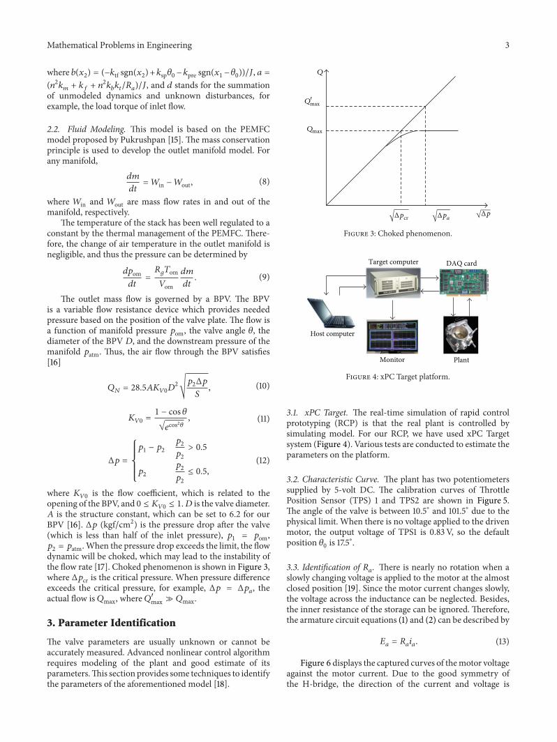
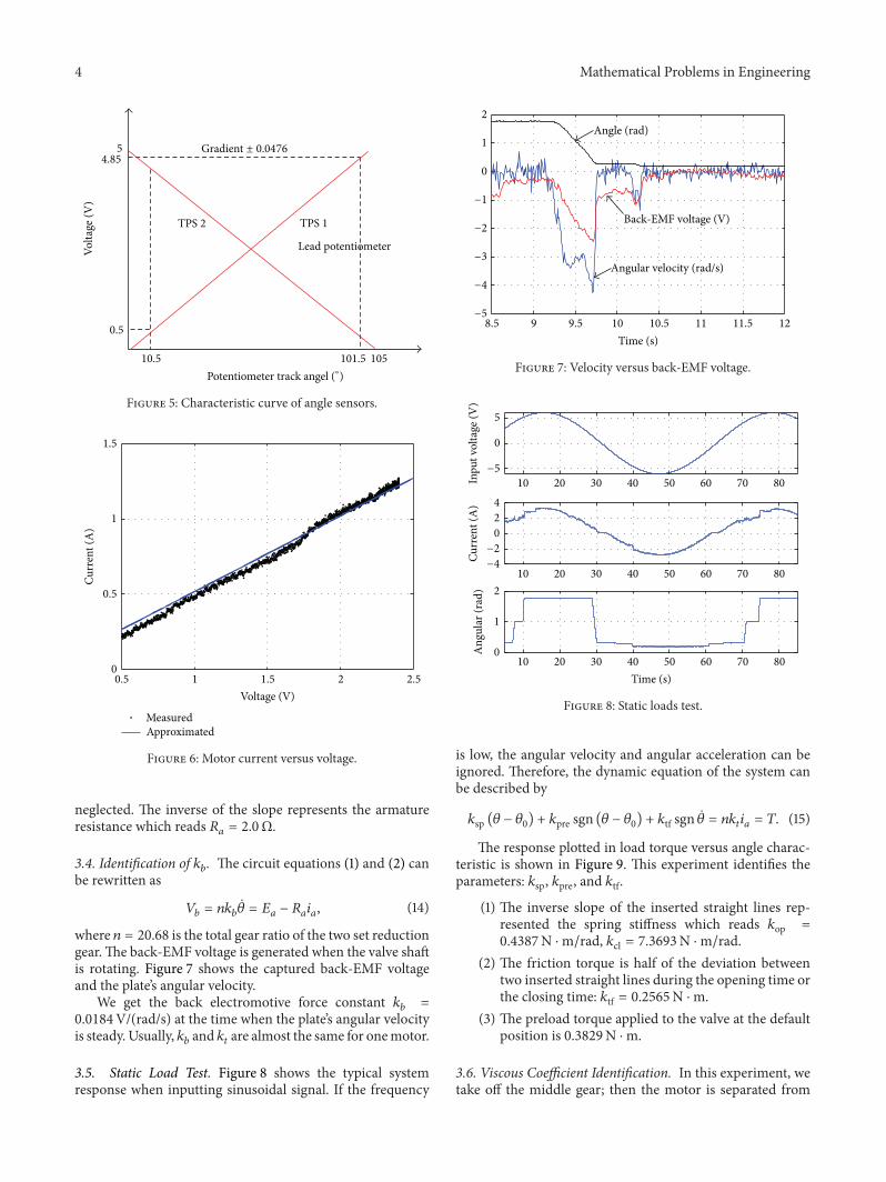
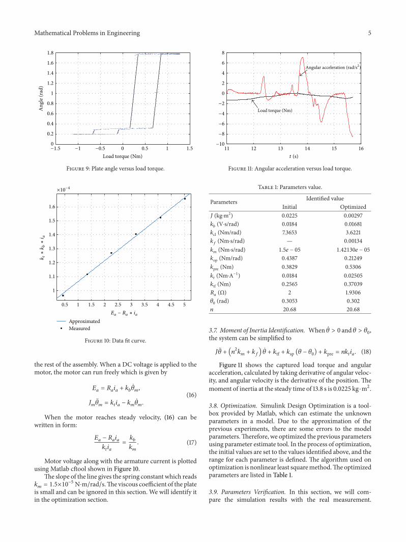
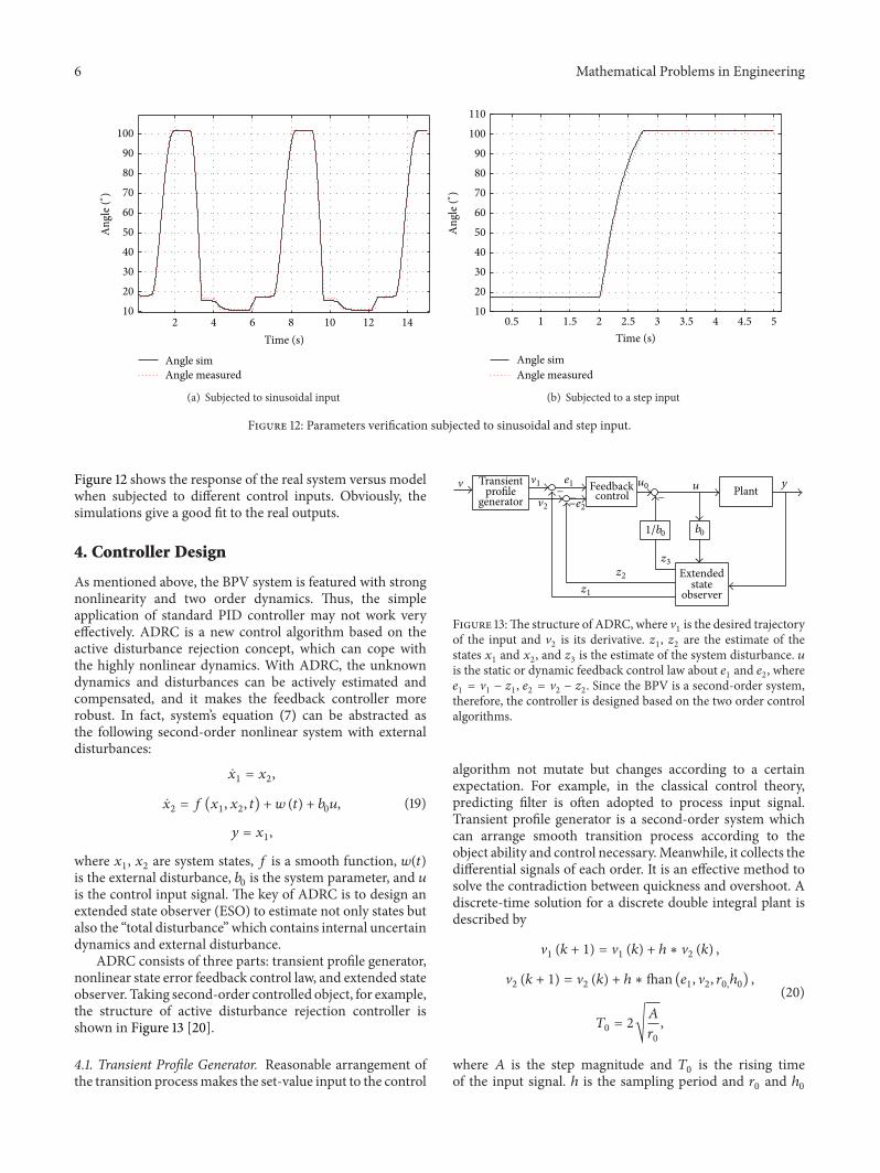
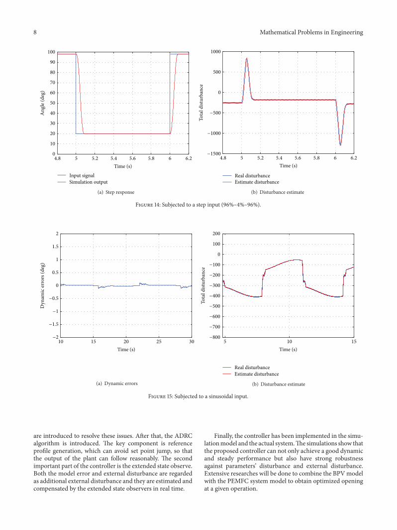
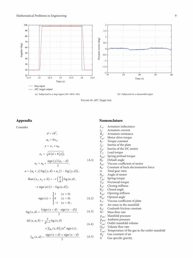