Experimental Identification of GHM and ADF … IDENTIFICATION OF GHM AND ADF ... material 3M ISD112...

III European Conference on Computational MechanicsSolids, Structures and Coupled Problems in Engineering

C.A. Mota Soares et.al. (eds.)Lisbon, Portugal, 5–8 June 2006

EXPERIMENTAL IDENTIFICATION OF GHM AND ADFPARAMETERS FOR VISCOELASTIC DAMPING MODELING

C. M. A. Vasques1, R. A. S. Moreira2 and J. Dias Rodrigues1

1Faculdade de Engenharia da Universidade do PortoDepartamento de Engenharia Mecanica e Gestao Industrial

Rua Dr. Roberto Frias s/n, 4200-465 Porto, PortugalE-mail: cvasques,[email protected]

2Universidade de AveiroDepartamento de Engenharia Mecanica

Campus Santiago, 3810-193 Aveiro, PortugalE-mail: [email protected]

Keywords: Viscoelastic, measurement, complex modulus, GHM, ADF, finite element, damp-ing, 3M ISD112.

Abstract. The implementation of the Golla-Hughes-McTavish (GHM) and Anelastic Displace-ment Fields (ADF) models in a general finite element (FE) model with viscoelastic dampingis presented and discussed in this paper. Additionally, a direct frequency analysis (DFA) isalso described and employed. A methodology to identify the complex shear modulus of theviscoelastic materials is described. The identified complex shear modulus of the viscoelasticmaterial 3M ISD112 is curve-fitted in order to obtain the modeling parameters of the GHMand ADF models. A sandwich plate with a viscoelastic core and elastic skins is analyzed. Mea-sured and predicted frequency response functions (FRFs) are compared with the purpose ofassessing the performance of the presented damping models. The analysis allows to asses thevalidity of the methodology to determine the frequency dependent complex modulus, the GHMand ADF parameters identification and the outcomes and drawbacks of the DFA, GHM andADF viscoelastic damping modeling strategies.

1 INTRODUCTION

Nowadays, in certain technological areas (e.g., automotive, aeronautics, aerospace, acous-tics) there is a growing need of lighter and stiffer structural components. However, the weightreduction, maintaining the rigidity unaffected, might lead to a significant reduction of the in-herent damping capacity of those flexible structures. Viscoelastic materials can be used as aneffective means of controlling the dynamics of structures, reducing and controlling the struc-tural vibrations and noise radiation from structures. They can be used in surface mounted orembedded damping treatments, utilizing passive viscoelastic materials alone, the so-called pas-sive treatments, or in an unified way with active materials such as piezoelectrics, the so-called

1

C. M. A. Vasques, R. A. S. Moreira and J. Dias Rodrigues

hybrid treatments. The use of these materials in damping treatments provides high dampingcapability over wide temperature and frequency ranges.

Applications with passive treatments alone, have been widely used since the end of the1950s, as can be found in reference textbooks (e.g., [1–4]). However, hybrid treatments area class of treatments usually more expensive and difficult to implement, but with the advantageof leading to a higher damping performance. Therefore, a considerable research effort has beenundertaken towards their effective use in real life applications. A review of hybrid treatments isaddressed in [5–8] and some analytical and experimental studies concerning beams, plates andshells can be found, for example, in [9–18].

In the last decade the technology associated with a more refined design and adequate im-plementation of viscoelastic-based damping treatments has achieved a relative maturity and isstarting to be frequently applied in practice by the scientific community and its industrial part-ners. In order to adequately design these viscoelastic damping treatments the viscoelastic mate-rial properties need to be accurately measured and considered for the underlying mathematicalmodels. The temperature and frequency dependent material properties of the viscoelastic mate-rials complicate the mathematical model and make the solution of the problem more difficult toobtain. Usually, isothermal conditions are assumed and only the frequency dependent constitu-tive behavior is taken into account. The simplest way of modeling these materials is achieved bya complex modulus approach (CMA) where the material properties are defined for each discretefrequency value [19, 20]. The CMA is also associated with the so-called modal strain energy(MSE) method [21] where the loss factors of each individual mode are determined from theratios between the dissipated modal strain energy of the viscoelastic counterpart and the storagemodal strain energy of the global structural system. The MSE method is known to lead to poorviscoelastic damping estimation of highly damped structural systems. Furthermore, the CMAis a frequency domain method that is limited to steady state vibrations and single-frequencyharmonic excitations. Thus, to account for the frequency dependent material properties, itera-tive versions of the MSE have been used successfully for moderate damping values [22]. Timedomain models, relying on internal variables (see [23]), such as the Golla-Hughes-McTavish(GHM) [24, 25] and anelastic displacement fields (ADF) [26, 27], or others [28, 29], utilizingadditional dissipation variables, have been successfully utilized and yield good damping esti-mates. Alternatively, the use of fractional calculus (FC) [30, 31] models, based upon the useof fractional derivatives, has the drawback of generating a ”non-standard” finite element (FE)formulation, with a more complex characteristic solution procedure, but yielding also gooddamping estimates. Other relevant contribution for the viscoelastic damping modeling is givenby Adhikari’s work [32] and his references therein. Regarding the temperature effects, stud-ies taking into account the temperature dependence of the properties and the self-heating ofviscoelastic materials have been performed by Lesieutre and his co-workers [33, 34] which ex-tended the ADF model for these cases leading, however, to nonlinear differential equations. Theeffects of the operating temperature on hybrid damping treatments performance and viscoelasticdamping efficiency were analyzed, for example, in [35–39].

The extensive use of passive or hybrid treatments using viscoelastic materials to reduce vi-bration and sound radiation from structures has motivated the integration of the aforementionedviscoelastic damping models into commercial or home-made FE codes, which is a very com-mon tool for studying complex structures used by the major part of the structural designers.Time domain models represent better alternatives to CMA-based models allowing the reductionof the computational burden and the study of the transient response in a more straightforwardmanner, even for highly damped structural systems. Among the time domain models, internal

2


variables models are more interesting from the computational point of view and easiness ofimplementation into FE codes. Thus, the GHM and ADF models are alternative methods, usedto model the damping behavior of viscoelastic materials in FE analysis, which yield a standardFE formulation (however with the addition of some ”non-physical” dissipative variables). Inorder to use them, one needs the GHM and ADF characteristic parameters which allow char-acterizing the complex (frequency dependent) constitutive behavior of the viscoelastic materialbeing used. To do that, experimental procedures to measure the isotropic constitutive behavior(usually the shear modulus) and numerical identification procedures of the measured data needto be developed.

In the open literature works concerning the experimental measurement of the viscoelasticconstitutive behavior by different approaches (test configurations) can be found, for example,in [1, 4, 40] and the references therein, where viscoelastic material master curves, tables andempirical and fractional derivative analytical expressions of the complex modulus and shiftfactor are presented for several types of viscoelastic materials. As referred by Jones [4], thatinformation is provided from various sources and is fairly accurate, in general, but it is by nomeans the best data which can be obtained. It is, however, the best data available in the publicdomain, and better data (”real” data) may be obtained only by additional testing or purchase ofdata from a data base (e.g, [41, 42]), often at considerable cost.

This paper addresses the experimental identification of the GHM and ADF parameters tobe used for modeling the viscoelastic damping behavior. The viscoelastic material consideredis this work is the 3M ISD112 [43], which was chosen because of its commercial availability,although the methodology described below can be applied to any viscoelastic material. Asreported by Trindade and Benjeddou [7] these parameters, in general, are adjusted by a curve-fitting of the viscoelastic material master curves, in order to minimize the difference betweenthe measured and estimated data. Lesieutre and Bianchini [26] presented the curve-fitting ofthe 3M ISD112 material data, at a temperature of 27 C, in the frequency range [8− 8000] Hz.They concluded that five ADF (with two parameters per ADF) represent exactly the behaviorof the material shear modulus and the loss factor. Friswell, Inman, and Lam [44] presented thesame analysis for the GHM model, with three or four parameters per model. They used the3M ISD112 material at 20 C in the frequency-range [10− 4800] Hz and DYAD601 material at24 C in the frequency range [2− 4800] Hz. Their results indicated that the model with fourparameters represented the material data better than that with three parameters. In general,GHM and ADF models fit well the master curves of materials whose properties have strongfrequency dependence. Nevertheless, the number of parameters needed is somehow relatedwith the degree of frequency dependence of the material properties and usually increases withthat dependence. That is why Enelund and Lesieutre [45] proposed a combination of the ADFmodel with the fractional derivatives model, where the relaxation equation for the anelasticstrain is taken as an in time differential equation of fractional-order, combining the best featuresof the ADF model and the FC. It was shown that this fractional-order ADF model can predictthe instantaneous transient response of the material over a wide frequency range using a singleanelastic strain field (only one ADF serie) governed by a fractional-order equation with thedrawback of yielding a ”non-standard” FE formulation requiring a more complex characteristicsolution procedure typical of FC.

In this work the implementation of the GHM and ADF models in a FE model is first pre-sented and discussed. Next, the experimental test rig and methodology used to identify thecomplex shear modulus of the viscoelastic material 3M ISD112 is described. An analytical em-pirical expression for the complex modulus and the shift factor obtained by curve fitting master

3


curves of 3M ISD112 is given in [40]. However, the accuracy of these expressions is not clearand with time manufacturers change the production process, with implications in the propertiesof the viscoelastic materials, making old data not so appropriate. Thus, that justifies the newexperimental methodology to estimate new data presented in this work. Then, the curve-fittedviscoelastic material data is compared with the measured one and the parameters of the GHMand ADF models are presented and used to represent the frequency dependent viscoelastic stiff-ness and to model the viscoelastic damping behavior of the structure. The identified parametersare then utilized in a FE model analysis and validated by comparison of frequency responsefunctions (FRFs) measured in a sandwich plate with a viscoelastic core and elastic skins.

The main contributions and novelties of this work are related with the fact that both mea-sured and predicted results are utilized to validate the methodologies to include viscoelasticdamping in FE models. Additionally, a new experimental procedure to determine the viscoelas-tic material properties is presented and discussed, and the characteristic material parametersof the GHM and ADF models of the 3M ISD112 are obtained by curve-fitting the measuredshear storage modulus and loss factor of ”actual” 3M ISD112 material. Furthermore, the ex-perimental data is usually taken by a ”manual” procedure from the plot of the nomogram givenby the manufacturer. Moreover, Trindade et al. [22] compared the GHM, ADF and interac-tive MSE models, however without comparing the predicted results with any measured (real)or predicted results obtained by a direct frequency analysis (DFA) approach, which is the mostprocessing time consuming technique, however the most precise. Therefore, the methodologiesare assessed and compared in a more rigorous way.

2 VISCOELASTIC DAMPING MODELING

2.1 Linear Viscoelasticity

Viscoelastic materials are rubber-like polymers possessing stiffness and damping character-istics which vary strongly with temperature and frequency. This polymers are materials com-posed of long intertwined and cross-linked molecular chains, each containing thousands or evenmillions of atoms. The internal molecular interactions that occur during deformation in general,and vibration in particular, give rise to macroscopic properties such as stiffness and energy dis-sipation during cyclic deformation, which in turn characterizes the mechanism of viscoelasticdamping.

It is well known that the viscoelastic constitutive behavior relies on the hypotheses that thecurrent value of the stress tensor depends upon the complete past history of the components ofthe strain tensor. Thus, considering an isotropic viscoelastic material under isothermal condi-tions, the theory of linear viscoelasticity [46] states that the constitutive relationship (in shearor extension) for a one-dimensional stress-strain system can be written as

σ(t) = G(t)ε(0) +

∫ t

0

G(t− τ)∂ε(τ)

∂τdτ , (1)

where the strain history ε(t) is restricted to be zero for t < 0, σ(t) is the resultant stress (shearor extensional) and G(t) is a constitutive time varying relaxation function. This gives rise to ahysteretic or complex modulus description for the vibration of a structure with viscoelastic ma-terial components.Thus, considering initial conditions equal to zero, i.e., ε(0) = 0, the Laplacetransform of Equation (1) yields

σ(s) = sG(s)ε(s), (2)

4


Table 1: GHM and ADF relaxation functions.

Function Author (year)

h(s) =n∑

i=1

αis2 + 2ζ iωis

s2 + 2ζ iωis + ω2i

Golla, McTavish and Hughes (1985, 1993)[24, 25]

h(s) =n∑

i=1

s∆i

s + Ωi

Lesieutre (1992) [48]

where sG(s) is a material modulus function which in turn can be represented by the equalitysG(s) = G0 [1 + h(s)] and substituted into (2) yielding

σ(s) = G0 [1 + h(s)] ε(s), (3)

where G0 is the relaxed (or static) shear modulus obtained after the material relaxation, i.e.,G0 = limt→∞G(t). Thus, since G0 is constant, the term G0ε(s) represents the recoverable(elastic) counterpart of the material stress while G0h(s)ε(s) represents the non-recoverable en-ergy dissipation effects (relaxation). For that reason, h(s) is usually termed as dissipation orrelaxation function.

Many authors have proposed different mathematical representations of the relaxation be-havior h(s) in the last decades, which in turn leads to different mathematical models of theviscoelastic damping behavior and different solution methods of the governing equations. Thedifferent relaxation functions are summarized in [7, 24, 32, 47] as a result of a compilation fromseveral works, where the different models and solution methods of the resultant mathematicalmodels are thoroughly discussed. Some of the most well known frequently referred in the openliterature are the internal variables GHM and ADF models, which will be considered in thiswork and described in the following sections, and the correspondent relaxation functions arepresented in Table 1.

2.2 Complex Modulus Approach

There are practical situations in which structures with viscoelastic materials may be sub-jected to steady-state oscillatory conditions. Under these conditions, assuming s as pure imag-inary variable, s = jω, the previously derived stress-strain relationship sG(s) in Equation (2),referring to the shear constitutive term, might be expressed as a function of the frequency ω inthe complex form

G(jω) = G′(ω) + jG′′(ω), (4)

where G′(ω) is the shear storage modulus, which accounts for the recoverable energy, andG′′(ω) is the shear loss modulus, which represents the energy dissipation effects [1, 4, 46]. Theloss factor of the viscoelastic materials is defined as

η(ω) =G′′(ω)

G′(ω), (5)

which alternatively allows to write Equation (4) as

G(jω) = G′(ω) [1 + jη(ω)] . (6)

5


For a linear, homogeneous and isotropic viscoelastic material, equivalent representations ofthe previous equations hold for the extensional modulus E(jω) and the relationship

G(jω) =E(jω)

2 [1 + ν(jω)], (7)

where ν(jω) is the Poisson’s ratio, establishes a relationship between the two. However, forsimplicity, a real frequency independent Poisson’s ratio ν(jω) = ν is assumed, which turns theloss factors of the shear and extensional complex moduli equal, i.e., ηE(ω) = ηG(ω) = η(ω).

2.3 Finite Element Implementation

2.3.1 Direct Frequency Analysis Response Model

Considering the frequency dependent physical properties of the viscoelastic materials pre-sented in the previous sections, the general time dependent FE equations of motion of a vis-coelastically damped general structural elastic system can be written as

Mu(t) + Du(t) + [KE + KV (jω)]u(t) = F(t), (8)

where M and D are the global mass and viscous proportional damping matrices, KE andKV (jω) are the elastic and viscoelastic stiffness matrices, and u(t) and F(t) are the displace-ments degrees of freedom (DoFs) and applied loads vectors. It’s worthy to mention that twotypes of damping models are considered in the previous equation: a frequency dependent hys-teretic (viscoelastic) damping type, represented by KV (jω), whose terms are complex and fre-quency dependent, representative of the viscoelastic relaxation behavior; and a viscous propor-tional damping type, which is described by D, representing other general sources of damping(e.g., the material damping of the elastic part of the structural system, air-based damping, energydissipation in the supports, etc.), which are assumed to be proportional to the velocity.

Using Equation (8) as it is, the frequency dependent matrix definition implies its use andanalysis only in the frequency domain, based in the CMA, where the material properties of thestiffness matrix of the viscoelastic layers are defined for each discrete frequency value [20, 49].Thus, the CMA is a frequency domain method where the frequency response model (FRFs) canbe generated in a straightforward manner from the results of many discrete frequency calcula-tions of the equations of motion, in which the complex stiffness matrix of the viscoelastic layersis re-calculated at each frequency value of the desired discrete frequency range.

Considering simple harmonic mechanical excitation,

F(t) = Fejωt, (9)

where F is the vector of applied loads amplitudes, the steady state mechanical harmonic re-sponse of the system can be written as

u(t) = Uejωt, (10)

where U is the vector response of displacement amplitudes. Substituting (9) and (10) into (8)yields

[K(jω) + jωD− ω2M]U = F, (11)

where K(jω) = KE + KV (jω), from which the complex solution vector U can be obtained.

6


The FRF (frequency response function) for a load applied in the ith DoF and a displacementDoF output o, can be obtained by solving (11) for different values of frequency,

[K(jωl) + jωlD− ω2l M]U(jωl) = Fi, (12)

where Fi denotes a force vector with a non-zero component in the ith DoF and all other elementsequal to zero, and U(jωl) is the resulting complex response vector (displacements) solution atfrequency ωl. Thus, the receptance FRF at frequency ωl, Hoi(jωl), is given by

Hoi(jωl) =Uo(jωl)

Fi

, (13)

where Fi is the amplitude of the load input and Uo(jωl) is the displacement amplitude extractedfrom the oth DoF of the vector U(jωl).

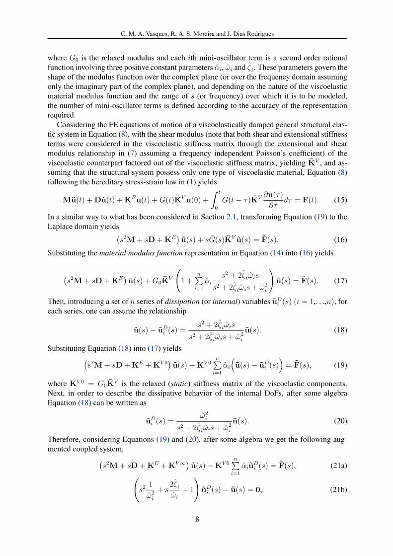
Finally, the FRF can be generated from the results of many discrete frequency calculations ofEquation (12), in which the complex stiffness matrix of the viscoelastic layers is re-calculatedat each frequency value of the discrete frequency range ω = ω0, . . . , ωl, . . . , ωf , as depicted inFigure 1.

( ) ( )E Vj jω ω= +K K K

2[ ( ) ] ( ) ij jw jω ω ω+ − =K D MU F

lω ω=

( )oiH jw

0, , , ,l fω ω ω ω= … …

Figure 1: Direct frequency analysis (DFA) response model generation diagram.

2.3.2 GHM Damping Model

When general transient responses are required, time domain models are more suitable andversatile and represent better alternatives to the CMA since they allow the reduction of thecomputational burden due to the recalculation of the stiffness matrix for each discrete frequencyvalue. One alternative is the GHM (Golla-Hughes-McTavish) model [24, 25] which assumesthe material modulus function sG(s) represented in terms of a series of mini-oscillator terms(Table 1),

sG(s) = G0 [1 + h(s)] = G0

(1 +

n∑i=1

αis2 + 2ζ iωis


), (14)

7


where G0 is the relaxed modulus and each ith mini-oscillator term is a second order rationalfunction involving three positive constant parameters αi, ωi and ζ i. These parameters govern theshape of the modulus function over the complex plane (or over the frequency domain assumingonly the imaginary part of the complex plane), and depending on the nature of the viscoelasticmaterial modulus function and the range of s (or frequency) over which it is to be modeled,the number of mini-oscillator terms is defined according to the accuracy of the representationrequired.

Considering the FE equations of motion of a viscoelastically damped general structural elas-tic system in Equation (8), with the shear modulus (note that both shear and extensional stiffnessterms were considered in the viscoelastic stiffness matrix through the extensional and shearmodulus relationship in (7) assuming a frequency independent Poisson’s coefficient) of theviscoelastic counterpart factored out of the viscoelastic stiffness matrix, yielding KV , and as-suming that the structural system possess only one type of viscoelastic material, Equation (8)following the hereditary stress-strain law in (1) yields

Mu(t) + Du(t) + KEu(t) + G(t)KV u(0) +

∫ t

0

G(t− τ)KV ∂u(τ)

∂τdτ = F(t). (15)

In a similar way to what has been considered in Section 2.1, transforming Equation (19) to theLaplace domain yields(

s2M + sD + KE)u(s) + sG(s)KV u(s) = F(s). (16)

Substituting the material modulus function representation in Equation (14) into (16) yields

(s2M + sD + KE

)u(s) + G0K

V

(1 +

n∑i=1

αis2 + 2ζ iωis


)u(s) = F(s). (17)

Then, introducing a set of n series of dissipation (or internal) variables uDi (s) (i = 1,. . .,n), for

each series, one can assume the relationship

u(s)− uDi (s) =

s2 + 2ζ iωis


u(s). (18)

Substituting Equation (18) into (17) yields(s2M + sD + KE + KV 0

)u(s) + KV 0

n∑i=1

αi

(u(s)− uD

i (s))

= F(s), (19)

where KV 0 = G0KV is the relaxed (static) stiffness matrix of the viscoelastic components.

Next, in order to describe the dissipative behavior of the internal DoFs, after some algebraEquation (18) can be written as

uDi (s) =

ω2i


u(s). (20)

Therefore, considering Equations (19) and (20), after some algebra we get the following aug-mented coupled system,(

s2M + sD + KE + KV∞) u(s)−KV 0n∑

i=1

αiuDi (s) = F(s), (21a)(

s2 1

ω2i

+ s2ζ i

ωi

+ 1

)uD

i (s)− u(s) = 0, (21b)

8


whereKV∞ =

(1 +

n∑i=1

αi

)KV 0.

In order to obtain the time-dependent behavior of the augmented system, multiplying Equation(21b) by αiK

V 0 and since all matrices are independent of s, a linear time domain model iseasily recovered by the inverse Laplace transform of Equations (21), yielding

Mu(t) + Du(t) +(KE + KV∞) u(t)−KV 0

n∑i=1

αiuDi (t) = F(t), (22a)

αi

ω2i

KV 0uDi (t) +

2αiζ i

ωi

KV 0uDi (t) + αiK

V 0uDi (t)− αiK

V 0u(t) = 0. (22b)

The augmented coupled system in Equations (22) might also be expressed in compact matrixform as

M¨q(t) + D ˙q(t) + Kq(t) = F(t), (23)

where

M =

[M 00 MDD

], D =

[D 00 DDD

], K =

[KEE KED

KDE KDD

],

q(t) = col[u(t), uD

1 (t), . . . , uDn (t)

], F(t) = col [F(t),0, . . . ,0] ,

and

MDD = diag( α1

ω21

KV 0, . . . ,αn

ω2n

KV 0)

, DDD = diag(2α1ζ1

ω1

KV 0, . . . ,2αnζn

ωn

KV 0)

,

KDD = diag(α1K

V 0, . . . ,α1KV 0)

, KED =[−α1K

V 0, . . . ,− αnKV 0]

,

KEE = KE + KV∞, KDE = KTED.

2.3.3 ADF Damping Model

A time domain model based on a variation, or Laplace transformed, formulation of the ADF(Anelastic Displacement Fields) model, originally proposed by Lesieutre and his co-workers[26, 27], is proposed in this work. It takes a definition of a complex modulus in the frequency(or Laplace) domain and utilizes the so-called internal, dissipation or anelastic (after Lesieu-tre) variables to simplify the equations, although with the drawback of increasing the size ofthe problem. Afterward, through an inverse Laplace transform one obtains an amenable andcomputationally tractable augmented system of linear ordinary differential equations that canbe solved by standard (linear) numerical procedures. With this procedure the FE model im-plementation of the ADF model is more straightforward when compared with the Lesieutre’soriginal direct time domain formulation based on the methods of irreversible thermodynamicsand a decomposition of the total displacement field in an elastic and anelastic counterpart.

Therefore, the process of deriving the augmented coupled elastic-anelastic (using the originaldesignation of Lesieutre) is similar to what has been presented for the GHM method, howeverutilizing a different definition of the material modulus function, and only some key steps willbe presented here. Thus, as reported by Lesieutre, the frequency dependent viscoelastic shear

9


modulus described by the ADF model, represented by a series of functions in the Laplacedomain, has the form [26, 48] (cf. Table 1)

sG(s) = G0 [1 + h(s)] = G0

(1 +

n∑i=1

∆is

s + Ωi

), (24)

where again G0 = limt→∞G(t) is the relaxed (or static, low-frequency) shear modulus, Ωi

is the inverse of the characteristic relaxation time at constant strain and ∆i the correspondentrelaxation resistance. To take into consideration the relaxation behavior, the entire ADF modelitself may be comprised of several individual fields where n series of ADF are used to describethe material behavior. Given measured values of the shear modulus in the form of frequencydependent complex modulus G(jω), the relaxed shear modulus G0 and the series of materialparameters ∆i and Ωi can be determined using curve fitting or optimization techniques. Thenumber of series of ADF parameters determines the accuracy of the matching of the measureddata over the frequency range of interest.

Substituting Equation (24) into (16) yields

(s2M + sD + KE

)u(s) + G0K

V

(1 +

n∑i=1

∆is

s + Ωi

)u(s) = F(s). (25)

Then, in a similar way, introducing a set of n series of anelastic (or internal, dissipation) uAi (s)

(i = 1,. . .,n) variables, for each series, one can assume the relationship

u(s)− uAi (s) =

s

s + Ωi

u(s). (26)

Substituting Equation (26) into (25), considering the dissipative behavior of the anelastic DoFsgiven by from Equation (26) as

uAi (s) =

Ωi

s + Ωi

u(s), (27)

after some algebra one gets the following augmented elastic-anelastic coupled system,(s2M + sD + KE + KV∞) u(s)−KV 0

n∑i=1

∆iuAi (s) = F(s), (28a)( s

Ωi

+ 1)uA

i (s)− u(s) = 0, (28b)

where this timeKV∞ =

(1 +

n∑i=1

∆i

)KV 0.

The time-dependent behavior of the augmented system, multiplying Equation (28b) by ∆iKV 0,

is recovered by the inverse Laplace transform of Equations (28), yielding

Mu(t) + Du(t) +(KE + KV∞) u(t)−KV 0

n∑i=1

∆iuAi (t) = F(t), (29a)

∆i

Ωi

KV 0 ˙uAi (t) + ∆iK

V 0uAi (t)−∆iK

V 0u(t) = 0. (29b)

10


The augmented coupled system in Equations (29) might be expressed in compact matrixform as in Equation (23) where for the ADF model one gets

M =

[M 00 0

], D =

[D 00 DAA

], K =

[KEE KEA

KAE KAA

],

q(t) = col[u(t), uA

1 (t), . . . , uAn (t)

], F(t) = col [F(t),0, . . . ,0] ,

where

DAA = diag(∆1

Ω1

KV 0, . . . ,∆n

Ωn

KV 0)

, KAA = diag(∆1K

V 0, . . . ,∆nKV 0)

,

KEE = KE + KV∞, KEA =[−∆1K

V 0, . . . , −∆nKV 0]

, KAE = KTEA.

2.3.4 State Space Design and Model Reduction

As can be seen in Equations (22) and (29), the main disadvantage of GHM and ADF modelsis that, associated with a FE discretization and in order to account for the frequency dependenceof the viscoelastic material, they lead to large systems, since they add auxiliary DoFs, whichfor each GHM or ADF series must be equal to the number of elastic DoFs. However, modelreduction techniques might be utilized in order to reduce the size of the system. As suggestedin [22] the matrices corresponding to the internal DoFs might be reduced and diagonalizedthrough a projection in a suitable reduced modal base, to reduce the computational cost. Theadvantages of this alternative (transformed) representation are that in the case where only somepart of the structure has surface mounted or embedded viscoelastic layers, only some FEs haveviscoelastic components and KV 0 can have several rows and columns of zeros, which in turnleads to some nill eigenvalues. Thus, through an adequate coordinate transformation based onthe eigenvalues and eigenvectors of KV 0 and elimination of the nil (spurious) eigenvalues thesize of the problem can be substantially smaller. Furthermore truncated complex state spacemodal models might also be used in order to reduce the system size even further. Moreover, onemay notice from M that when compared with the GHM model the anelastic DoFs of the ADFmodel have no inertia and therefore the global mass matrix M is singular and is not positive-definite. However, the singularity of the mass matrix can be overcome if, instead of solvingthe second-order system (23) of the ADF, a state-space representation with an adequate designof the state variables is considered. The number of flexible modes is kept the same and thedissipative modes, which correspond to the internal relaxations of the viscoelastic material, areoverdamped with low observability. The reader is referred to [22, 47, 50, 51] for further detailsabout state space design and model reduction techniques.

3 EXPERIMENTAL IDENTIFICATION OF VISCOELASTIC MATERIALS

3.1 Underlying Analytical Model

The proposed experimental methodology for the dynamic characterization of the complexmodulus of viscoelastic materials is based on the direct identification of the complex equiva-lent stiffness K(jω) of a discrete single degree of freedom (SDoF) system [52]. The complexstiffness is physically materialized by a thin viscoelastic layer which is subjected to cyclic sheardeformation imposed by a dynamic exciter. The dynamic response of the considered SDoF sys-tem is then used to evaluate the shear storage modulus and loss factor variation with frequencyand temperature.

11


The receptance FRF of the SDoF system, assuming stationary harmonic motion, is given by

H(jω) =X

F=

1

K(jω)− ω2M, (30)

where F and X are the amplitudes of the dynamic force and displacement response and M is themass. The complex value stiffness K(jω) of the viscoelastic sample can be directly determinedthrough the inverse of the receptance, the dynamic stiffness function Z(jω) = H−1(jω), as

K(jω) = ω2M + Z(jω). (31)

The viscoelastic material storage modulus G′(ω) and loss factor η(ω) functions can then beevaluated from

G′(ω) =h

AS

(ω2M − Re [Z(jω)]

), (32a)

η(ω) =Im [Z(jω)]

ω2M + Re [Z(jω)], (32b)

where h is the thickness of the viscoelastic sample and AS its shear area.

3.2 Experimental Apparatus

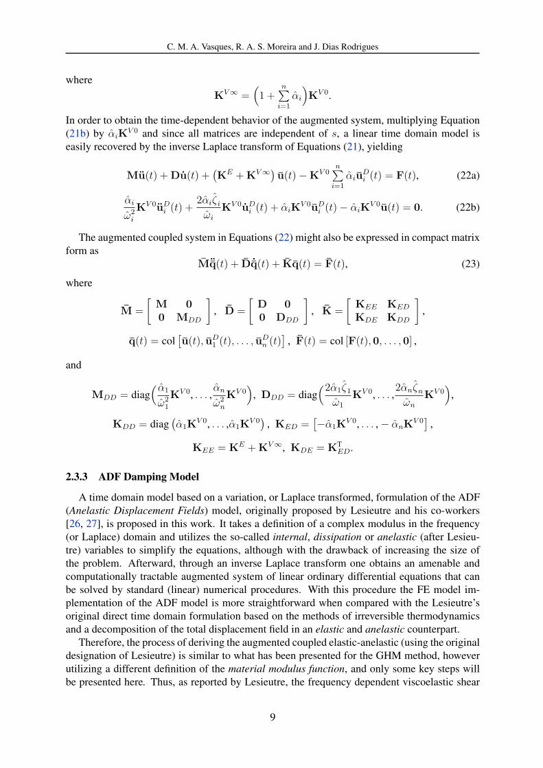
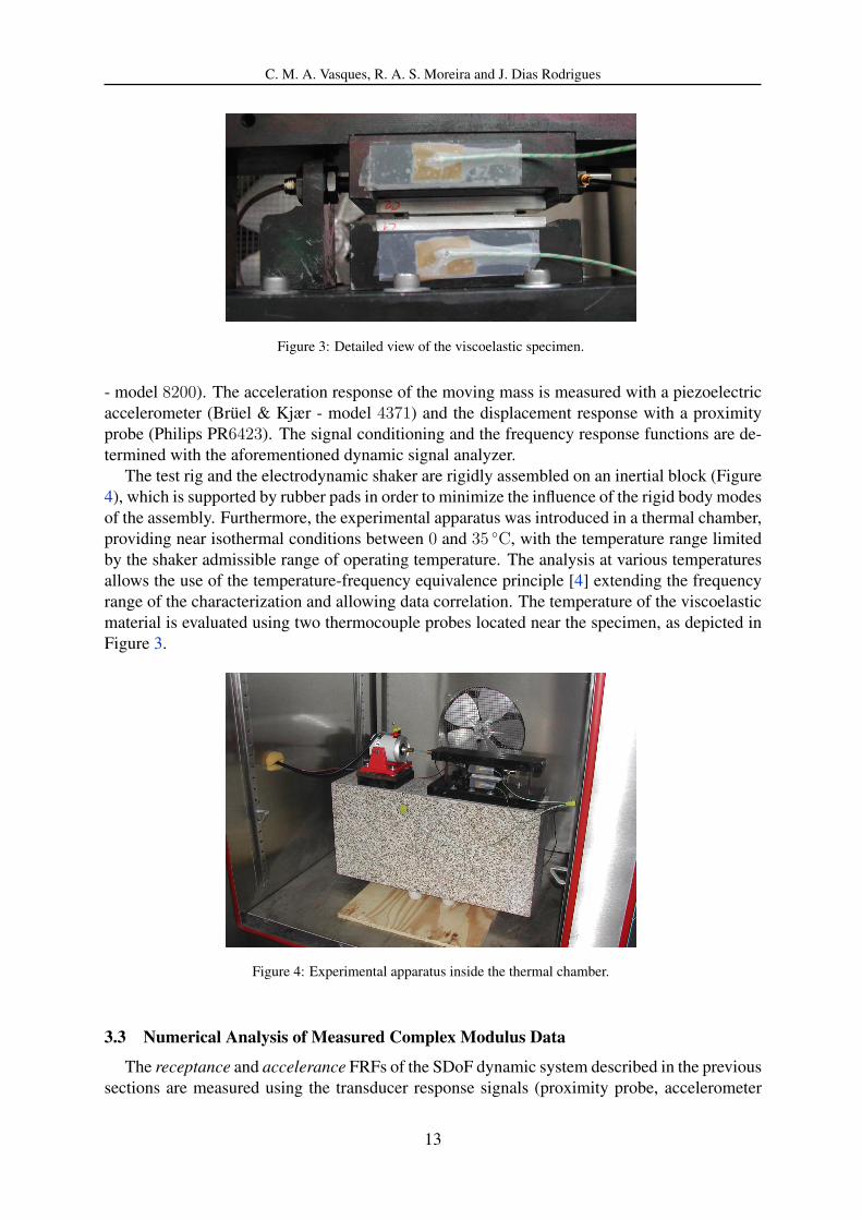
The test rig representing the dynamic SDoF system used to identify the complex shear mod-ulus of viscoelastic materials is illustrated in Figure 2. The underlying analytical model of thecomplex SDoF system previously described comprises a moving mass M , represented by theupper bar (2), and a complex stiffness K(jω), represented by the thin viscoelastic layer sam-ple (4) introduced between two rigid blocks, as shown in Figure 3. The upper bar is guidedby two thin lamina springs (3), which provide the restraint of the spurious DoFs, allowing theviscoelastic specimen to deform mainly in shear due to the relative motion between the movingbar (2) and the fixed bar (1).

Figure 2: Test rig used to identify the complex shear modulus.

The dynamic excitation of the moving bar is provided by an electrodynamic shaker (Ling Dy-namic Systems - model 201), using a thin stinger to minimize the rotation and lateral excitation,driven by a random signal generated by the signal generator of a dynamic signal analyzer (Bruel& Kjær - model 2035) and amplified at a power amplifier (Ling Dynamic Systems - PA25E).The applied excitation force is measured using a piezoelectric force transducer (Bruel & Kjær

12


Figure 3: Detailed view of the viscoelastic specimen.

- model 8200). The acceleration response of the moving mass is measured with a piezoelectricaccelerometer (Bruel & Kjær - model 4371) and the displacement response with a proximityprobe (Philips PR6423). The signal conditioning and the frequency response functions are de-termined with the aforementioned dynamic signal analyzer.

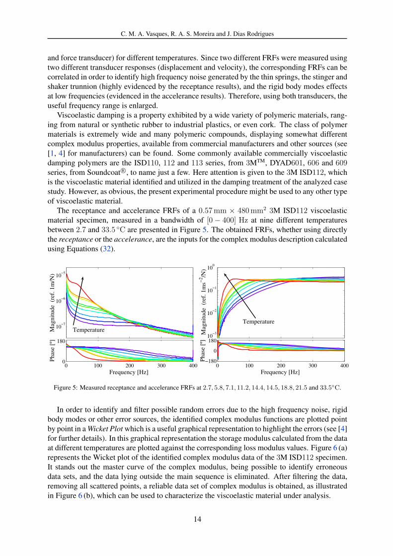
The test rig and the electrodynamic shaker are rigidly assembled on an inertial block (Figure4), which is supported by rubber pads in order to minimize the influence of the rigid body modesof the assembly. Furthermore, the experimental apparatus was introduced in a thermal chamber,providing near isothermal conditions between 0 and 35 C, with the temperature range limitedby the shaker admissible range of operating temperature. The analysis at various temperaturesallows the use of the temperature-frequency equivalence principle [4] extending the frequencyrange of the characterization and allowing data correlation. The temperature of the viscoelasticmaterial is evaluated using two thermocouple probes located near the specimen, as depicted inFigure 3.

Figure 4: Experimental apparatus inside the thermal chamber.

3.3 Numerical Analysis of Measured Complex Modulus Data

The receptance and accelerance FRFs of the SDoF dynamic system described in the previoussections are measured using the transducer response signals (proximity probe, accelerometer

13


and force transducer) for different temperatures. Since two different FRFs were measured usingtwo different transducer responses (displacement and velocity), the corresponding FRFs can becorrelated in order to identify high frequency noise generated by the thin springs, the stinger andshaker trunnion (highly evidenced by the receptance results), and the rigid body modes effectsat low frequencies (evidenced in the accelerance results). Therefore, using both transducers, theuseful frequency range is enlarged.

Viscoelastic damping is a property exhibited by a wide variety of polymeric materials, rang-ing from natural or synthetic rubber to industrial plastics, or even cork. The class of polymermaterials is extremely wide and many polymeric compounds, displaying somewhat differentcomplex modulus properties, available from commercial manufacturers and other sources (see[1, 4] for manufacturers) can be found. Some commonly available commercially viscoelasticdamping polymers are the ISD110, 112 and 113 series, from 3MTM, DYAD601, 606 and 609series, from Soundcoat R©, to name just a few. Here attention is given to the 3M ISD112, whichis the viscoelastic material identified and utilized in the damping treatment of the analyzed casestudy. However, as obvious, the present experimental procedure might be used to any other typeof viscoelastic material.

The receptance and accelerance FRFs of a 0.57 mm × 480 mm2 3M ISD112 viscoelasticmaterial specimen, measured in a bandwidth of [0− 400] Hz at nine different temperaturesbetween 2.7 and 33.5 C are presented in Figure 5. The obtained FRFs, whether using directlythe receptance or the accelerance, are the inputs for the complex modulus description calculatedusing Equations (32).

0 100 200 300 400 0

180

Phas

e [º

]

Frequency [Hz]

10−7

10−6

10−5

Mag

nitu

de (

ref.

1m

/N)

Temperature

0 100 200 300 400−180

0

180

Phas

e [º

]

Frequency [Hz]

10−3

10−2

10−1

100

Mag

nitu

de (

ref.

1m

s−2 /N

)

Temperature

Figure 5: Measured receptance and accelerance FRFs at 2.7, 5.8, 7.1, 11.2, 14.4, 14.5, 18.8, 21.5 and 33.5C.

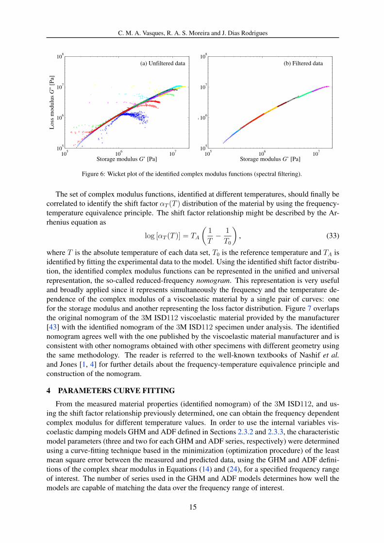
In order to identify and filter possible random errors due to the high frequency noise, rigidbody modes or other error sources, the identified complex modulus functions are plotted pointby point in a Wicket Plot which is a useful graphical representation to highlight the errors (see [4]for further details). In this graphical representation the storage modulus calculated from the dataat different temperatures are plotted against the corresponding loss modulus values. Figure 6 (a)represents the Wicket plot of the identified complex modulus data of the 3M ISD112 specimen.It stands out the master curve of the complex modulus, being possible to identify erroneousdata sets, and the data lying outside the main sequence is eliminated. After filtering the data,removing all scattered points, a reliable data set of complex modulus is obtained, as illustratedin Figure 6 (b), which can be used to characterize the viscoelastic material under analysis.

14


105

106

107

105

106

107

108

Los

s m

odul

us G

" [P

a]

Storage modulus G’ [Pa]

(a) Unfiltered data

105

106

107

105

106

107

108

Storage modulus G’ [Pa]

Stor

age

mod

ulus

G"

[Pa]

(b) Filtered data

Figure 6: Wicket plot of the identified complex modulus functions (spectral filtering).

The set of complex modulus functions, identified at different temperatures, should finally becorrelated to identify the shift factor αT (T ) distribution of the material by using the frequency-temperature equivalence principle. The shift factor relationship might be described by the Ar-rhenius equation as

log [αT (T )] = TA

(1

T− 1

T0

), (33)

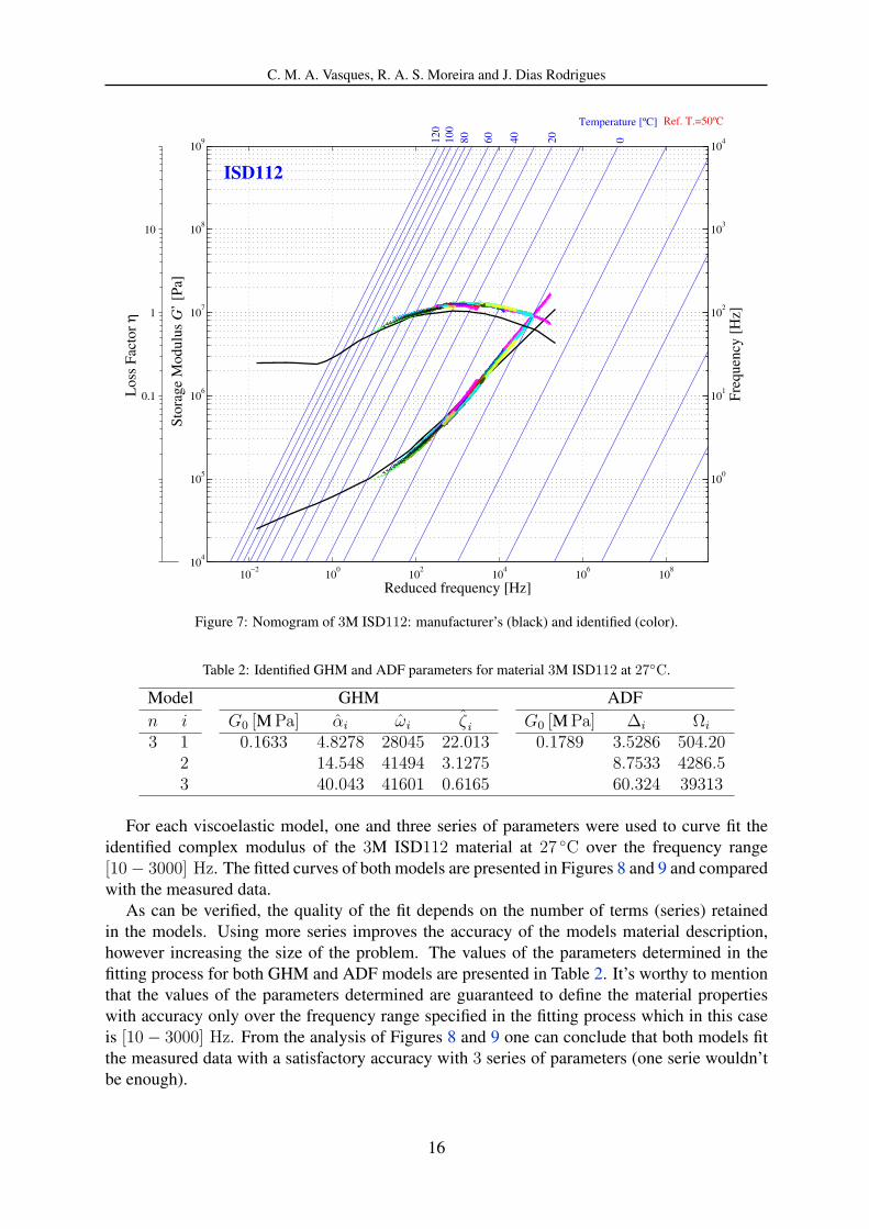
where T is the absolute temperature of each data set, T0 is the reference temperature and TA isidentified by fitting the experimental data to the model. Using the identified shift factor distribu-tion, the identified complex modulus functions can be represented in the unified and universalrepresentation, the so-called reduced-frequency nomogram. This representation is very usefuland broadly applied since it represents simultaneously the frequency and the temperature de-pendence of the complex modulus of a viscoelastic material by a single pair of curves: onefor the storage modulus and another representing the loss factor distribution. Figure 7 overlapsthe original nomogram of the 3M ISD112 viscoelastic material provided by the manufacturer[43] with the identified nomogram of the 3M ISD112 specimen under analysis. The identifiednomogram agrees well with the one published by the viscoelastic material manufacturer and isconsistent with other nomograms obtained with other specimens with different geometry usingthe same methodology. The reader is referred to the well-known textbooks of Nashif et al.and Jones [1, 4] for further details about the frequency-temperature equivalence principle andconstruction of the nomogram.

4 PARAMETERS CURVE FITTING

From the measured material properties (identified nomogram) of the 3M ISD112, and us-ing the shift factor relationship previously determined, one can obtain the frequency dependentcomplex modulus for different temperature values. In order to use the internal variables vis-coelastic damping models GHM and ADF defined in Sections 2.3.2 and 2.3.3, the characteristicmodel parameters (three and two for each GHM and ADF series, respectively) were determinedusing a curve-fitting technique based in the minimization (optimization procedure) of the leastmean square error between the measured and predicted data, using the GHM and ADF defini-tions of the complex shear modulus in Equations (14) and (24), for a specified frequency rangeof interest. The number of series used in the GHM and ADF models determines how well themodels are capable of matching the data over the frequency range of interest.

15


10−2

100

102

104

106

108

104

105

106

107

108

109

Stor

age

Mod

ulus

G’

[Pa]

Reduced frequency [Hz]

020406080100

120

Temperature [ºC] Ref. T.=50ºC

100

101

102

103

104

Freq

uenc

y [H

z]

ISD112

0.1

1

10

Los

s Fa

ctor

η

Figure 7: Nomogram of 3M ISD112: manufacturer’s (black) and identified (color).

Table 2: Identified GHM and ADF parameters for material 3M ISD112 at 27C.

Model GHM ADFn i G0 [M Pa] αi ωi ζ i G0 [M Pa] ∆i Ωi

3 1 0.1633 4.8278 28045 22.013 0.1789 3.5286 504.202 14.548 41494 3.1275 8.7533 4286.53 40.043 41601 0.6165 60.324 39313

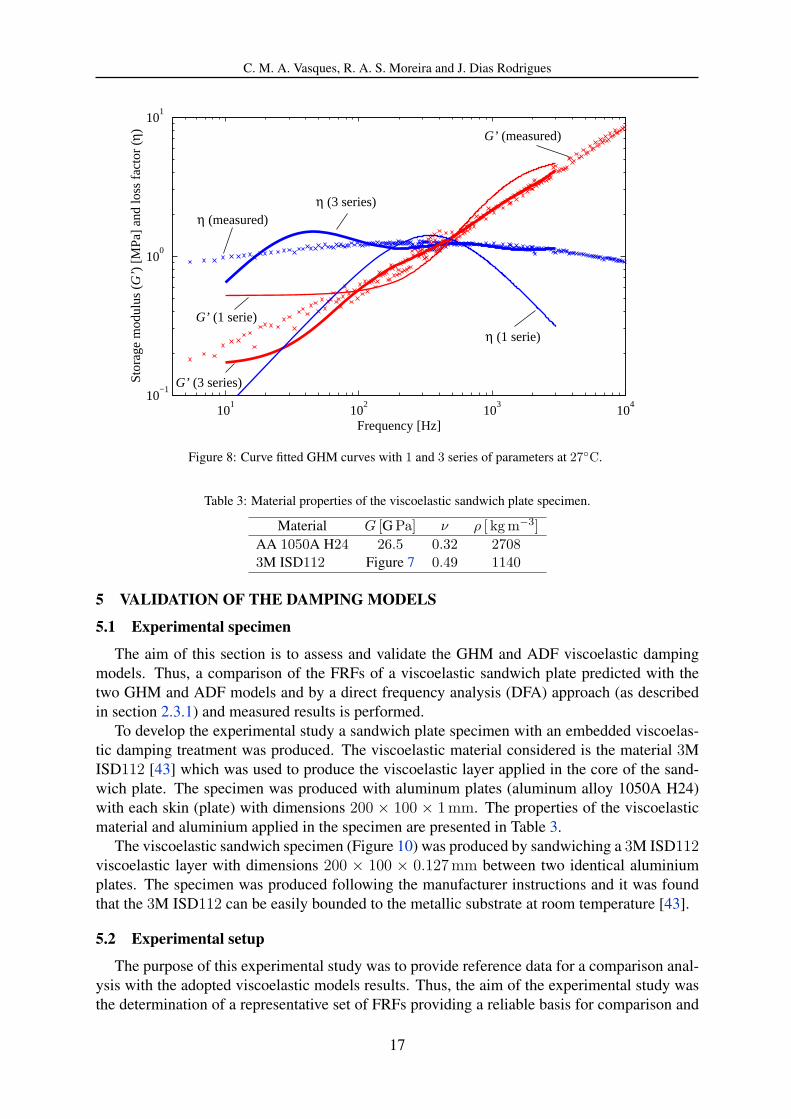
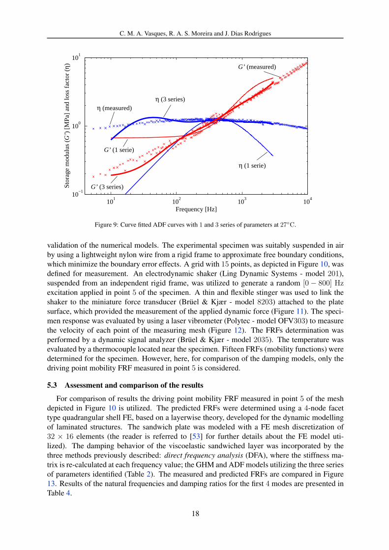
For each viscoelastic model, one and three series of parameters were used to curve fit theidentified complex modulus of the 3M ISD112 material at 27 C over the frequency range[10− 3000] Hz. The fitted curves of both models are presented in Figures 8 and 9 and comparedwith the measured data.

As can be verified, the quality of the fit depends on the number of terms (series) retainedin the models. Using more series improves the accuracy of the models material description,however increasing the size of the problem. The values of the parameters determined in thefitting process for both GHM and ADF models are presented in Table 2. It’s worthy to mentionthat the values of the parameters determined are guaranteed to define the material propertieswith accuracy only over the frequency range specified in the fitting process which in this caseis [10− 3000] Hz. From the analysis of Figures 8 and 9 one can conclude that both models fitthe measured data with a satisfactory accuracy with 3 series of parameters (one serie wouldn’tbe enough).

16


101

102

103

104

10−1

100

101

Frequency [Hz]

Stor

age

mod

ulus

(G

’) [

MPa

] an

d lo

ss f

acto

r (η

)

G’ (1 serie)

G’ (3 series)

G’ (measured)

η (1 serie)

η (3 series)η (measured)

Figure 8: Curve fitted GHM curves with 1 and 3 series of parameters at 27C.

Table 3: Material properties of the viscoelastic sandwich plate specimen.

Material G [G Pa] ν ρ [ kg m−3]AA 1050A H24 26.5 0.32 27083M ISD112 Figure 7 0.49 1140

5 VALIDATION OF THE DAMPING MODELS

5.1 Experimental specimen

The aim of this section is to assess and validate the GHM and ADF viscoelastic dampingmodels. Thus, a comparison of the FRFs of a viscoelastic sandwich plate predicted with thetwo GHM and ADF models and by a direct frequency analysis (DFA) approach (as describedin section 2.3.1) and measured results is performed.

To develop the experimental study a sandwich plate specimen with an embedded viscoelas-tic damping treatment was produced. The viscoelastic material considered is the material 3MISD112 [43] which was used to produce the viscoelastic layer applied in the core of the sand-wich plate. The specimen was produced with aluminum plates (aluminum alloy 1050A H24)with each skin (plate) with dimensions 200 × 100 × 1 mm. The properties of the viscoelasticmaterial and aluminium applied in the specimen are presented in Table 3.

The viscoelastic sandwich specimen (Figure 10) was produced by sandwiching a 3M ISD112viscoelastic layer with dimensions 200 × 100 × 0.127 mm between two identical aluminiumplates. The specimen was produced following the manufacturer instructions and it was foundthat the 3M ISD112 can be easily bounded to the metallic substrate at room temperature [43].

5.2 Experimental setup

The purpose of this experimental study was to provide reference data for a comparison anal-ysis with the adopted viscoelastic models results. Thus, the aim of the experimental study wasthe determination of a representative set of FRFs providing a reliable basis for comparison and

17


101

102

103

104

10−1

100

101

Frequency [Hz]

Stor

age

mod

ulus

(G

’) [

MPa

] an

d lo

ss f

acto

r (η

)

G’ (1 serie)

G’ (3 series)

G’ (measured)

η (1 serie)

η (3 series)η (measured)

Figure 9: Curve fitted ADF curves with 1 and 3 series of parameters at 27C.

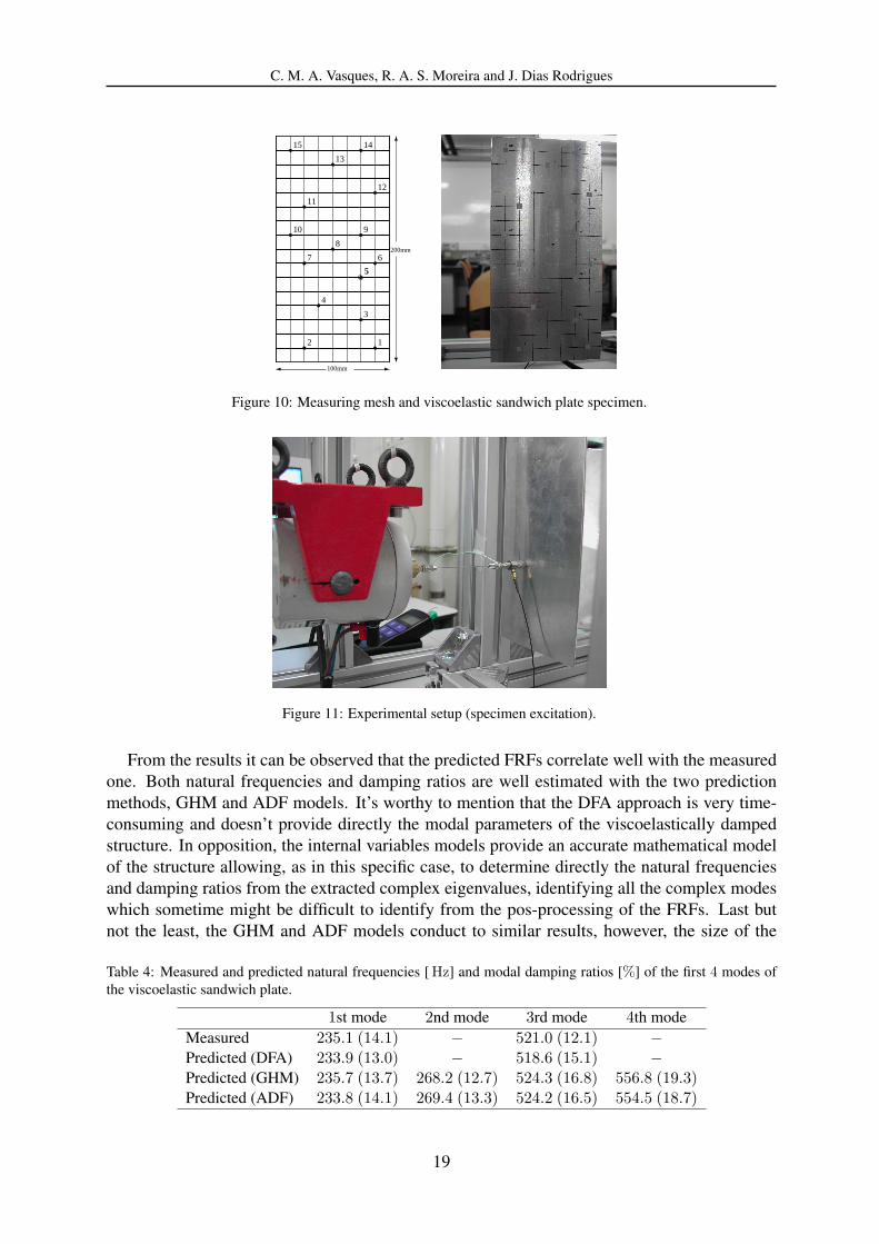
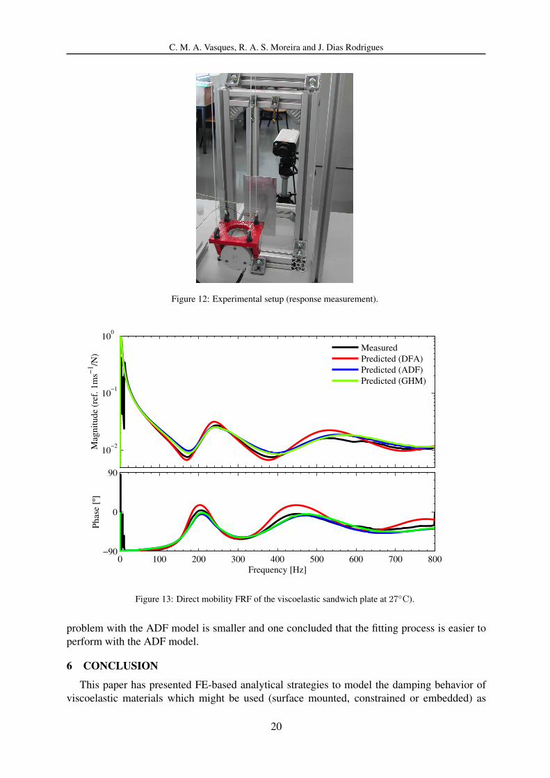
validation of the numerical models. The experimental specimen was suitably suspended in airby using a lightweight nylon wire from a rigid frame to approximate free boundary conditions,which minimize the boundary error effects. A grid with 15 points, as depicted in Figure 10, wasdefined for measurement. An electrodynamic shaker (Ling Dynamic Systems - model 201),suspended from an independent rigid frame, was utilized to generate a random [0− 800] Hzexcitation applied in point 5 of the specimen. A thin and flexible stinger was used to link theshaker to the miniature force transducer (Bruel & Kjær - model 8203) attached to the platesurface, which provided the measurement of the applied dynamic force (Figure 11). The speci-men response was evaluated by using a laser vibrometer (Polytec - model OFV303) to measurethe velocity of each point of the measuring mesh (Figure 12). The FRFs determination wasperformed by a dynamic signal analyzer (Bruel & Kjær - model 2035). The temperature wasevaluated by a thermocouple located near the specimen. Fifteen FRFs (mobility functions) weredetermined for the specimen. However, here, for comparison of the damping models, only thedriving point mobility FRF measured in point 5 is considered.

5.3 Assessment and comparison of the results

For comparison of results the driving point mobility FRF measured in point 5 of the meshdepicted in Figure 10 is utilized. The predicted FRFs were determined using a 4-node facettype quadrangular shell FE, based on a layerwise theory, developed for the dynamic modellingof laminated structures. The sandwich plate was modeled with a FE mesh discretization of32 × 16 elements (the reader is referred to [53] for further details about the FE model uti-lized). The damping behavior of the viscoelastic sandwiched layer was incorporated by thethree methods previously described: direct frequency analysis (DFA), where the stiffness ma-trix is re-calculated at each frequency value; the GHM and ADF models utilizing the three seriesof parameters identified (Table 2). The measured and predicted FRFs are compared in Figure13. Results of the natural frequencies and damping ratios for the first 4 modes are presented inTable 4.

18


Rui A.S. Moreira and José Dias Rodrigues

3.2 Experimental setup

As stated above, the experimental study developed in this work had two distinct purposes:to provide a comparison analysis between the damping efficiency and the flexural stiffnessachieved for each treatment, and to validate the model adopted for the numerical analysispresented in the following section. For both purposes, the aim of the experimental study wasthe determination of a representative set of frequency response functions providing the inputdata for a modal parameter identification process and, on the other hand, a reliable basis for thenumerical layerwise model [5, 6] validation for a direct frequency analysis using the complexmodulus approach [4].

To obtain free boundary conditions, which minimize the boundary error effects, theexperimental specimens were suspended by a thin nylon wire from a rigid frame. A meshwith 15 measuring points, as depicted in Figure3, was defined for all the tested specimens.

12

3

4

5

67

8

910

11

12

13

1415

¾ -100mm?

6

200mm

Figure 3.Measuring mesh and specimen boundary conditions

An electrodynamic shaker (Ling Dynamic Systems - model 201), suspended from anindependent rigid frame, was utilized to generate a random ([0-800]Hz) excitation in point 5of each specimen. A thin and flexible stinger was used to link the shaker to the miniatureforce transducer (Brüel & Kjær - model 8203) attached to the plate surface, which provided themeasurement of the applied dynamic force (Figure4). The specimens responses were evaluatedby using a laser vibrometer (Polytec - model OFV303) to measure the velocity of each pointof the measuring mesh (Figure5). The temperature of the measurement was evaluated by athermocouple located near the specimens.

5

Figure 10: Measuring mesh and viscoelastic sandwich plate specimen.

Figure 11: Experimental setup (specimen excitation).

From the results it can be observed that the predicted FRFs correlate well with the measuredone. Both natural frequencies and damping ratios are well estimated with the two predictionmethods, GHM and ADF models. It’s worthy to mention that the DFA approach is very time-consuming and doesn’t provide directly the modal parameters of the viscoelastically dampedstructure. In opposition, the internal variables models provide an accurate mathematical modelof the structure allowing, as in this specific case, to determine directly the natural frequenciesand damping ratios from the extracted complex eigenvalues, identifying all the complex modeswhich sometime might be difficult to identify from the pos-processing of the FRFs. Last butnot the least, the GHM and ADF models conduct to similar results, however, the size of the

Table 4: Measured and predicted natural frequencies [ Hz] and modal damping ratios [%] of the first 4 modes ofthe viscoelastic sandwich plate.

1st mode 2nd mode 3rd mode 4th modeMeasured 235.1 (14.1) − 521.0 (12.1) −Predicted (DFA) 233.9 (13.0) − 518.6 (15.1) −Predicted (GHM) 235.7 (13.7) 268.2 (12.7) 524.3 (16.8) 556.8 (19.3)Predicted (ADF) 233.8 (14.1) 269.4 (13.3) 524.2 (16.5) 554.5 (18.7)

19


Figure 12: Experimental setup (response measurement).

10−2

10−1

100

Mag

nitu

de (

ref.

1m

s−1 /N

)

0 100 200 300 400 500 600 700 800−90

0

90

Frequency [Hz]

Phas

e [º

]

MeasuredPredicted (DFA)Predicted (ADF)Predicted (GHM)

Figure 13: Direct mobility FRF of the viscoelastic sandwich plate at 27C).

problem with the ADF model is smaller and one concluded that the fitting process is easier toperform with the ADF model.

6 CONCLUSION

This paper has presented FE-based analytical strategies to model the damping behavior ofviscoelastic materials which might be used (surface mounted, constrained or embedded) as

20


damping treatments in structures. An experimental procedure to identify the complex shearmodulus of viscoelastic materials was presented and the obtained data was used to fit the internalvariables models GHM and ADF and identify their characteristic parameters for the 3M ISD112viscoelastic material. Measured and FE-based predicted FRFs based on a direct frequencyanalysis (DFA), GHM and ADF models, were compared in order to assess the damping modelsand validate the experimental procedure for the material properties identification and the curvefitting process.

The application of a discrete dynamic system, describing a SDoF analytical model, providesa reliable identification methodology, since it is based on the direct (in opposition to indirectmeasuring approaches based on vibrating beams) characterization of the complex stiffness of aviscoelastic material sample in shear deformation, providing results similar to those publishedby the material manufacturer.

Regarding the internal variables models under analysis here, which were implemented atthe FE model level, the ADF model is known to lead to an augmented model of the dampedstructural system with a lower size than the GHM model. To the opinion of the authors the ADFmodel represents the best alternative to accurately model the damping behavior since it yieldsgood trade-off between accuracy and complexity. One major disadvantage in using internalvariables models such as the GHM or ADF is the creation of additional dissipation (or anelastic)variables increasing the size of the coupled damped FE model. However, an alternative based onthe direct frequency analysis (DFA) using the FE spatial model and re-calculating the complexviscoelastic stiffness matrix for each discrete frequency value might be used with the outcomeof being simpler to implement and the drawback of being time-consuming and not providingdirectly the modal parameters of the damped structural system. All the models have similaraccuracy and yield representative results of viscoelastically damped structural systems.

7 ACKNOWLEDGMENTS

The funding given by Fundacao para a Ciencia e a Tecnologia of the Ministerio da Ciencia eda Tecnologia of Portugal under grant POSI SFRH/BD/13255/2003 is gratefully acknowledgedby the first author. Acknowledgements are also addressed to 3M Company for providing theviscoelastic materials used in this work.

REFERENCES

[1] A. Nashif, D. Jones and J. Henderson. Vibration Damping. John Wiley & Sons, NewYork, NY, 1985.

[2] C. T. Sun and Y. P. Lu. Vibration Damping of Structural Elements. Prentice Hall, Engle-wood Cliffs, NJ, 1995.

[3] D. J. Mead. Passive Vibration Control. John Wiley & Sons, Chichester, UK, 1998.

[4] D. I. G. Jones. Handbook of Viscoelastic Vibration Damping. John Wiley & Sons, Chich-ester, UK, 2001.

[5] C. H. Park and A. Baz. Vibration damping and control using active constrained layerdamping: A survey. The Shock and Vibration Digest, 31(5):355–364, 1999.

[6] A. Benjeddou. Advances in hybrid active-passive vibration and noise control via piezo-electric and viscoelastic constrained layer treatments. Journal of Vibration and Control, 7(4):565–602, 2001.

21


[7] M. A. Trindade and A. Benjeddou. Hybrid active-passive damping treatments using vis-coelastic and piezoelectric materials: Review and assessment. Journal of Vibration andControl, 8(6):699–745, 2002.

[8] R. Stanway, J. A. Rongong and N. D. Sims. Active constrained-layer damping: A state-of-the-art review. Proceedings of the Institution of Mechanical Engineers. Part I: Journalof Systems and Control Engineering, 217(6):437–456, 2003.

[9] B. Azvine, G. R. Tomlinson and R. J. Wynne. Use of active constrained-layer dampingfor controlling resonant vibration. Smart Materials and Structures, 4(1):1–6, 1995.

[10] J. Ro, A. El-Ali and A. Baz. Control of sound radiation from a fluid-loaded plate usingactive constrained layer damping. In N. S. Ferguson, H. F. Wolfe and C. Mei, editors,Proceedings of the Sixth International Conference on Recent Advances in Structural Dy-namics, pages 1252–1273, Southampton, UK, 1997.

[11] M. C. Ray and A. Baz. Optimization of energy dissipation of active constrained layerdamping treatments of plates. Journal of Sound and Vibration, 208(3):391–406, 1997.

[12] C. H. Park and A. Baz. Vibration control of bending modes of plates using active con-strained layer damping. Journal of Sound and Vibration, 227(4):711–734, 1999.

[13] Q. Liu, A. Chattopadhyay, H. Gu and X. Zhou. Use of segmented constrained layerdamping treatment for improved helicopter aeromechanical stability. Smart Materialsand Structures, 9(4):523, 2000.

[14] A. Baz. Active constrained layer damping of thin cylindrical shells. Journal of Sound andVibration, 240(5):921–935, 2001.

[15] C. Chantalakhana and R. Stanway. Active constrained layer damping of clamped-clampedplate vibrations. Journal of Sound and Vibration, 241(5):755, 2001.

[16] S. H. Ko, C. H. Park, H. C. Park and W. Hwang. Vibration control of an arc type shellusing active constrained layer damping. Smart Materials and Structures, 13(2):350, 2004.

[17] C. M. A. Vasques, B. R. Mace, P. Gardonio and J. D. Rodrigues. Arbitrary active con-strained layer damping treatments on beams: Finite element modelling and experimentalvalidation. Computers and Structures, 2005 (in press).

[18] C. M. A. Vasques and J. Dias Rodrigues. Adaptive feedforward control of vibration of abeam with active-passive damping treatments: Numerical analysis and experimental im-plementation. In Proceedings of the 16th International Conference on Adaptive Structuresand Technologies (ICAST 2005), pages 255–262. DEStech Publications, Paris, France,2006.

[19] R. A. Moreira and J. D. Rodrigues. The modelisation of constrained damping layer treat-ment using the finite element method: Spatial and viscoelastic behavior. In Proceedingsof the International Conference on Structural Dynamics Modelling: Test, Analysis Corre-lation and Validation, Madeira, Portugal, 2002.

[20] R. Moreira and J.D. Rodrigues. Constrained damping layer treatments: Finite elementmodeling. Journal of Vibration and Control, 10(4):575–595, 2004.

[21] C. D. Johnson, D. A. Kienholz and L. C. Rogers. Finite element prediction of dampingin beams with constrained viscoelastic layers. Shock and Vibration Bulletin, (1):71–81,1980.

22


[22] M. A. Trindade, A. Benjeddou and R. Ohayon. Modeling of frequency-dependent vis-coelastic materials for active-passive vibration damping. Journal of Vibration and Acous-tics, 122(2):169–174, 2000.

[23] A. R. Johnson. Modeling viscoelastic materials using internal variables. Shock and Vibra-tion Digest, 31(2):91–100, 1999.

[24] D. F. Golla and P. C. Hughes. Dynamics of viscoelastic structures a time-domain, finiteelement formulation. Jounal of Applied Mechanics, 52(12):897–906, 1985.

[25] D. J. McTavish and P. C. Hughes. Modeling of linear viscoelastic space structures. Journalof Vibration and Acoustics, 115(1):103–110, 1993.

[26] G. A. Lesieutre and E. Bianchini. Time domain modeling of linear viscoelasticity usinganelastic displacement fields. Journal of Vibration and Acoustics, 117(4):424–430, 1995.

[27] G. A. Lesieutre, E. Bianchini and A. Maiani. Finite element modeling of one-dimensionalviscoelastic structures using anelastic displacement fields. Journal of Guidance Controland Dynamics, 19(3):520–527, 1996.

[28] Y.C. Yiu. Finite element analysis of structures with classical viscoelastic materials. In 34thAIAA/ASME/ASCE/AHS/ASC Structures, Structural Dynamics and Materials Conference,volume 4, pages 2110–2119, La Jolla, CA, USA, 1993.

[29] L. A. Silva. Internal Variable and Temperature Modeling Behavior of Viscoelastic Struc-tures – A Control Analysis. PhD thesis, Virginia Tech, VA, USA, 2003.

[30] R. L. Bagley and P. J. Torvik. Fractional calculus - A different approach to the analysis ofviscoelastically damped structures. AIAA Journal, 21(5):741–748, 1983.

[31] R. L. Bagley and P. J. Torvik. Fractional calculus in the transient analysis of viscoelasti-cally damped structures. AIAA Journal, 23(6):918–925, 1985.

[32] S. Adhikari and J. Woodhouse. Quantification of non-viscous damping in discrete linearsystems. Journal of Sound and Vibration, 260(3):499–518, 2003.

[33] C. R. Brackbill, G. A. Lesieutre, E. C. Smith and K. Govindswamy. Thermomechanicalmodeling of elastomeric materials. Smart Materials & Structures, 5(5):529–539, 1996.

[34] G. A. Lesieutre and K. Govindswamy. Finite element modeling of frequency dependentand temperature-dependent dynamic behavior of viscoelastic materials in simple shear.International Journal of Solids and Structures, 33(3):419–432, 1996.

[35] A. Baz. Robust control of active constrained layer damping. Journal of Sound and Vibra-tion, 211(3):467–480, 1998.

[36] M. I. Friswell and D. J. Inman. Hybrid damping treatments in thermal environments.In G.R. Tomlinson and W.A. Bullough, editors, Smart Materials and Structures, pages667–674. IOP Publishing, Bristol, UK, 1998.

[37] M. A. Trindade, A. Benjeddou and R. Ohayon. Finite element analysis of frequency- andtemperature-dependent hybrid active-passive vibration damping. Revue Europeenne desElements Finis, 9(1-3):89–111, 2000.

[38] L. A. Silva, E. M. Austin and D. J. Inman. Time-varying controller for temperature-dependent viscoelasticity. Journal of Vibration and Acoustics, 127(3):215–222, 2005.

23


[39] V. Pradeep and N. Ganesan. Vibration behavior of acld treated beams under thermal envi-ronment. Journal of Sound and Vibration, 292(3-5):1036–1045, 2006.

[40] M. L. Drake and J. Soovere. A design guide for damping of aerospace structures. InAFWAL Vibration Damping Workshop, volume 3, 1984.

[41] M. L. Drake and G. E. Terborg. Polymeric material testing procedures to determine damp-ing properties and the results of selected commercial materials. Technical Report AFWAL-TR-80-4093, Materials Laboratory, Wright-Patterson Air Force Base, 1980.

[42] M. L. Drake. Damping properties of various materials. Technical Report AFWAL-TR-88-4248, Materials Laboratory, Wright-Patterson Air Force Base, 1988.

[43] 3M. Scotchdamp Vibration Control Systems: Product Information and Performance Data.3M Industrial Tape and Specialties Division, St. Paul, MN, USA, 1993.

[44] M. I. Friswell, D. J. Inman and M. J. Lam. On the realisation of GHM models in vis-coelasticity. Journal of Intelligent Material Systems and Structures, 8(11):986–993, 1997.

[45] M. Enelund and G. A. Lesieutre. Time domain modeling of damping using anelasticdisplacement fields and fractional calculus. International Journal of Solids and Structures,36(29):4447–4472, 1999.

[46] R. M. Christensen. Theory of Viscoelasticity: An Introduction. Academic Press, NewYork, 2nd edition, 1982.

[47] C. H. Park, D. J. Inman and M. J. Lam. Model reduction of viscoelastic finite elementmodels. Journal of Sound and Vibration, 219(4):619–637, 1999.

[48] G. A. Lesieutre. Finite elements for dynamic modeling of uniaxial rods with frequency-dependent material properties. International Journal of Solids and Structures, 29(12):1567–1579, 1992.

[49] C. M. A. Vasques, B. Mace, P. Gardonio and J. D. Rodrigues. Analytical formulationand finite element modelling of beams with arbitrary active constrained layer dampingtreatments. Institute of Sound and Vibration Research, Technical Memorandum TM934,2004.

[50] M. I. Friswell and D. J. Inman. Reduced-order models of structures with viscoelasticcomponents. AIAA Journal, 37(10):1318–1325, 1999.

[51] C. M. A. Vasques and J. Dias Rodrigues. Simulation of combined feedback/feedforwardactive control of vibration of beams with ACLD treatments. Computers and Structures,2006 (accepted).

[52] B. R. Allen. A direct complex stiffness test system for viscoelastic material properties. InProceedings of 3rd Smart Structures and Materials (SPIE), volume 2720, pages 338–345,San Diego, CA, USA, 1996.

[53] R. A. S. Moreira, J. D. Rodrigues and A. J. M. Ferreira. A generalized layerwise finiteelement for multi-layer damping treatments. Computational Mechanics, 37(5):426–444,2006.

24

Experimental Identification of GHM and ADF … IDENTIFICATION OF GHM AND ADF ... material 3M ISD112...

Documents

Transcript of Experimental Identification of GHM and ADF … IDENTIFICATION OF GHM AND ADF ... material 3M ISD112...