Research Article Dynamic Analysis and Chaos of the 4D ...

Research ArticleDynamic Analysis and Chaos of the 4D Fractional-OrderPower System

Fengyun Sun and Qin Li

School of Mathematics and Computational Science, Yantai University, Yantai 264005, China

Correspondence should be addressed to Fengyun Sun; [email protected]

Received 24 December 2013; Accepted 14 January 2014; Published 23 February 2014

Academic Editor: Xinguang Zhang

Copyright © 2014 F. Sun and Q. Li. This is an open access article distributed under the Creative Commons Attribution License,which permits unrestricted use, distribution, and reproduction in any medium, provided the original work is properly cited.

Now dealing with power system became the most important arts. In this paper we report the dynamic analysis of a fractional-orderpower system with parameter 𝑄

1. To the best know of our knowledge, that was the first report about bifurcation analysis of the

fractional order power system. So first we discuss the dynamic analysis with different fractional order and different parameters.Furthermore we will establish its numerical simulations which are provided to demonstrate the feasibility and efficacy of ouranalysis.

1. Introduction

For a long time, many researchers have been growing interestin investigating the potential use of dynamics in applica-tions, taking power system as an example. Under normaland emergency operating conditions, power systems alwayscan show rich nonlinear dynamic phenomena. From a math-ematical point of view, differential equations can be usedto describe the dynamic behavior of the power system. Thepower system is usually run under equilibrium conditions,but in engineering practice, the stability of the equilibriumpoint form sometimes changeswith the range of small pertur-bations. After 1980s, with the development of the power sys-tem, even if a small perturbation can also cause the system tolose stability, due to the changing of some control parameters.Researchers focus on the study of the critical state of thesystem.

Along with the 300-year-old history of the fractional cal-culus, its applications to electrical engineering have receivedmore attention. Typically, chaotic systems are still chaoticeven when their differential equations become fractional-order differential systems [1–9]. We all know there are manyresults on fractional-order system, but the bifurcation offractional-order nonlinear systems has not been well studied.

Obviously there are two kinds of methods which havebeen used in the previous paper to solve fractional-orderdifferential systems: the frequency-domain methods [10] andthe time-domain methods [11]. Some researcher found it issometimes invalid to research some chaotic systemswhousedthe frequently method to investigate chaos [12, 13]. However,we give up the first method and choice the time domainmethod to make the numerical simulations in this paper.Themain ideawas introduced byDiethelm et al. [14] and has beenused by the following paper [15–17].

In this paper, we report the first investigation of a frac-tional-order power system using the time domain method.Recently, a simplified 4D power system was reported byChiang et al. [18]. Its chaotic and bifurcation analysis havebeen investigated and got well results [19, 20]. But to thebest know of our knowledge, that was the first report aboutbifurcation analysis of the fractional-order system.Accordingto the different values we will show the bifurcation diagramsof the system which chaos exists.

The paper is organized as follows. In Section 2, thenumerical algorithm for the fractional-order power system ispresented. In Section 3, the chaotic behavior and bifurcationsof the system are studied. Finally, we summarize the results.

Hindawi Publishing CorporationAbstract and Applied AnalysisVolume 2014, Article ID 534896, 8 pageshttp://dx.doi.org/10.1155/2014/534896

2 Abstract and Applied Analysis

−10

1

−2

0

20

0.2

0.4

𝜔

𝛿

𝛿

𝛿m0

0.20.4

0.5

1

1.5−2

0

2

𝜔

�

0.1

0.20.3

0.5

1

0.6

0.8

1

1.2

𝛿m

�0.5

11.5

−1

0

1−2

0

2

𝜔

𝛿m�

(a)

0 2 4 6 8 10 120

0.05

0.1

0.15

0.2

0.25

0.3

0.35

0.4

0.45Bifurcation map

q1

|y|

whe

rex=y

(b)

Figure 1: (a) The 3D trajectory in the integer order power system. (b) The related bifurcation diagram of the parameter 𝑄1.

2. Numerical Algorithm for Fractional-OrderPower System

2.1. System Description [21]. In this paper we consider thefollowing power system in [21] (see Figure 1). Here we use𝑄1as the varying parameter to derive the corresponding

attractor.Now we consider the fraction order power system by

𝑑𝑞1𝛿𝑚

𝑑𝑡𝑞= 𝜔;

𝑑𝑞2𝜔

𝑑𝑡𝑞=50

3] sin (𝛿 − 𝛿

𝑚+ 0.0873) −

1

6𝜔 +

47

25;

𝑑𝑞3𝛿

𝑑𝑡𝑞= 496.8]2 −

50

3] cos (𝛿 − 𝛿

𝑚− 0.0873)

−2000

3] cos (𝛿 − 0.2094)

−280

3] +100

3𝑄1+130

3;

𝑑𝑞4]𝑑𝑡𝑞

= − 78.7]2 + 26.2] cos (𝛿 − 𝛿𝑚− 0.0124)

+524

5] cos (𝛿 − 0.1346) + 29

2] − 5.3𝑄

1−703

100;

(1)

Abstract and Applied Analysis 3

here 𝛿𝑚, 𝜔, 𝛿, and ] are variables and 𝑑𝑞𝑖/𝑑𝑡𝑞𝑖 = 𝐷

𝑞𝑖

∗(𝑖 =

1, 2, 3, 4), its order is denoted by 𝑞 = (𝑞1, 𝑞2, 𝑞3, 𝑞4). When

𝑞𝑖= 1, 𝑖 = 1, 2, 3, 4, system (1) becomes the integer order

power system in [21].

2.2. Fractional Derivative [22]. There are several definitionsof a fractional-order differential system. In the following, weintroduce the most common one of them [22]:

𝐷𝛼

∗𝑥 (𝑡) = 𝐽

𝑚−𝛼𝑥(𝑡)(𝑚), with 𝛼 > 0 (2)

with 𝑚 = [𝛼]; that is, 𝑚 is the first integer which is not lessthan 𝛼, 𝑥𝑚 is the m-order derivative in the usual sense, and𝐽𝛽 (𝛽 > 0) is the 𝛽-order Reimann-Liouville integral operatorwith expression

𝐽𝛽𝑦 (𝑡) =

1

Γ (𝛽)∫

𝑡

0

(𝑡 − 𝜏)𝛽−1𝑦 (𝜏) 𝑑𝜏. (3)

Here 𝜏 stands for Gamma function, and the operator 𝐷𝛼∗is

generally called “𝛼-order Caputo differential operator” [22].Next, we consider the fractional-order differential equa-

tion with related initial conditions

𝐷𝛼

∗𝑥 (𝑡) = 𝑓 (𝑡, 𝑥 (𝑡)) , 0 < 𝑡 < 𝑇,

𝑥(𝑘)(0) = 𝑥

(𝑘)

0, 𝑘 = 0, 1, 2, . . . 𝑛 − 1.

(4)

Combined with the methods [11, 14] and the abovedefinition of fractional-order differential equation. Set 𝜏 =𝑇/𝑁, the fractional-order power system can be rewritten

(𝛿𝑚)𝑛+1= (𝛿𝑚)0+

𝜏𝑞1

Γ (𝑞1+ 2)

×{

{

{

𝜔𝑝

𝑛+1+

𝑛

∑

𝑗=0

(𝑎1)𝑗,𝑛+1𝜔𝑗

}

}

}

;

𝜔𝑛+1= 𝜔0+

𝜏𝑞2

Γ (𝑞2+ 2)

× {50

3]𝑝𝑛+1

sin (𝛿𝑝𝑛+1− (𝛿𝑚)𝑝

𝑛+1+ 0.0873)

−1

6𝜔𝑝

𝑛+1+47

25

+

𝑛

∑

𝑗=0

(𝑎2)𝑗,𝑛+1

[50

3]𝑗sin (𝛿

𝑗− (𝛿𝑚)𝑗

+0.0873)

−1

6𝜔𝑗+47

25]} ;

𝛿𝑛+1= 𝛿0+

𝜏𝑞3

Γ (𝑞3+ 2)

× {496.8(]𝑝𝑛+1)2

−50

3]𝑝𝑛+1

× cos (𝛿𝑝𝑛+1− (𝛿𝑚)𝑝

𝑛+1− 0.0873)

−2000

3]𝑝𝑛+1

cos (𝛿𝑝𝑛+1− 0.2094) −

280

3]𝑝𝑛+1

+100

3𝑞1+130

3

+

𝑛

∑

𝑗=0

(𝑎3)𝑗,𝑛+1

[496.8(]𝑗)2

−50

3]𝑗

× cos (𝛿𝑗− (𝛿𝑚)𝑗− 0.0873)

−2000

3]𝑗

× cos (𝛿𝑗− 0.2094)

−280

3]𝑗+100

3𝑞1+130

3]} ;

]𝑛+1= ]0+

𝜏𝑞4

Γ (𝑞4+ 2)

× { − 78.7(]𝑝𝑛+1)2

− 26.2]𝑝𝑛+1

× cos (𝛿𝑝𝑛+1− (𝛿𝑚)𝑝

𝑛+1− 0.0124)

−524

5]𝑝𝑛+1

cos (𝛿𝑝𝑛+1− 0.1346)

+29

2]𝑝𝑛+1− 5.3𝑞

1−703

100

+

𝑛

∑

𝑗=0

(𝑎4)𝑗,𝑛+1

[ − 78.7(]𝑗)2

− 26.2]𝑗

× cos (𝛿𝑗− (𝛿𝑚)𝑗− 0.0124)

−524

5]𝑗cos (𝛿

𝑗− 0.1346)

+29

2]𝑗− 5.3𝑞

1−703

100]} ;

(5)

in which

(𝛿𝑚)𝑝

𝑛+1= (𝛿𝑚)0+

1

Γ (𝑞1)

𝑛

∑

𝑗=0

(𝑏1)𝑗,𝑛+1𝜔𝑗;

𝜔𝑝

𝑛+1= 𝜔0+

1

Γ (𝑞2)


×

𝑛

∑

𝑗=0

(𝑏2)𝑗,𝑛+1

[50

3]𝑗

× sin (𝛿𝑗− (𝛿𝑚)𝑗+ 0.0873)

−1

6𝜔𝑗+47

25] ;

𝛿𝑝

𝑛+1= 𝛿0+

1

Γ (𝑞3)

×

𝑛

∑

𝑗=0

(𝑏3)𝑗,𝑛+1

[496.8(]𝑗)2

−50

3]𝑗cos (𝛿

𝑗− (𝛿𝑚)𝑗− 0.0873)

−2000

3]𝑗cos (𝛿

𝑗− 0.2094)

−280

3]𝑗+100

3𝑞1+130

3] ;

]𝑝𝑛+1= ]0+

1

Γ (𝑞4)

×

𝑛

∑

𝑗=0

(𝑏4)𝑗,𝑛+1

[ − 78.7(]𝑗)2

− 26.2]𝑗

× cos (𝛿𝑗− (𝛿𝑚)𝑗− 0.0124)

−524

5]𝑗cos (𝛿

𝑗− 0.1346)

+29

2]𝑗− 5.3𝑞

1−703

100] ;

(6)

(𝑎1)𝑗,𝑛+1

=

{{

{{

{

𝑛𝑞1 − (𝑛 − 𝑞

1) (𝑛 + 1)

𝑞1 , 𝑗 = 0,

(𝑛 − 𝑗 + 2)𝑞1+1

+ (𝑛 − 𝑗)𝑞1+1

−2(𝑛 − 𝑗 + 1)𝑞1+1

, 0 ≤ 𝑗 ≤ 𝑛,

(𝑎2)𝑗,𝑛+1

=

{{

{{

{

𝑛𝑞2 − (𝑛 − 𝑞

2) (𝑛 + 1)

𝑞2 , 𝑗 = 0,

(𝑛 − 𝑗 + 2)𝑞2+1

+ (𝑛 − 𝑗)𝑞2+1

−2(𝑛 − 𝑗 + 1)𝑞2+1

, 0 ≤ 𝑗 ≤ 𝑛,

(𝑎3)𝑗,𝑛+1

=

{{

{{

{

𝑛𝑞3 − (𝑛 − 𝑞

3) (𝑛 + 1)

𝑞3 , 𝑗 = 0,

(𝑛 − 𝑗 + 2)𝑞3+1

+ (𝑛 − 𝑗)𝑞3+1

−2(𝑛 − 𝑗 + 1)𝑞3+1

, 0 ≤ 𝑗 ≤ 𝑛,

(𝑎4)𝑗,𝑛+1

=

{{

{{

{

𝑛𝑞4 − (𝑛 − 𝑞

4) (𝑛 + 1)

𝑞4 , 𝑗 = 0,

(𝑛 − 𝑗 + 2)𝑞4+1

+ (𝑛 − 𝑗)𝑞4+1

−2(𝑛 − 𝑗 + 1)𝑞4+1

, 0 ≤ 𝑗 ≤ 𝑛,

(7)

(𝑏1)𝑗,𝑛+1

=𝜏𝑞1

𝑞1

((𝑛 − 𝑗 + 1)𝑞1 − (𝑛 − 𝑗)

𝑞1) , 0 ≤ 𝑗 ≤ 𝑛,

(𝑏2)𝑗,𝑛+1

=𝜏𝑞2

𝑞2

((𝑛 − 𝑗 + 1)𝑞2 − (𝑛 − 𝑗)

𝑞2) , 0 ≤ 𝑗 ≤ 𝑛,

(𝑏3)𝑗,𝑛+1

=𝜏𝑞3

𝑞3

((𝑛 − 𝑗 + 1)𝑞3 − (𝑛 − 𝑗)

𝑞3) , 0 ≤ 𝑗 ≤ 𝑛,

(𝑏4)𝑗,𝑛+1

=𝜏𝑞4

𝑞4

((𝑛 − 𝑗 + 1)𝑞4 − (𝑛 − 𝑗)

𝑞4) , 0 ≤ 𝑗 ≤ 𝑛.

(8)

3. Bifurcations Analysis ofthe Fractional-Order Power System

3.1. Integer-Order Power System. In the following discus-sion, we mainly use the simulation method to analyze thefractional-order power system by calculating the largestLyapunov exponent using the Wolf algorithm [6]. Becausethe nonperiodicity solutions and sensitive dependence oninitial conditions are important reason of chaos, here, welet the initial condition be defined as ((𝛿

𝑚)0, 𝜔0, 𝛿0, ]0) =

(0.348; 0.1; 0.138; 0.925) [21] and vary 𝑞𝑖= 𝑞 (𝑖 = 1, 2, 3, 4).

According to our numerical simulations, we have visuallyfounded the difference between the integer order and thefractional order. Here we let 𝑞

𝑖= 1 (𝑖 = 1, 2, 3, 4), that is,

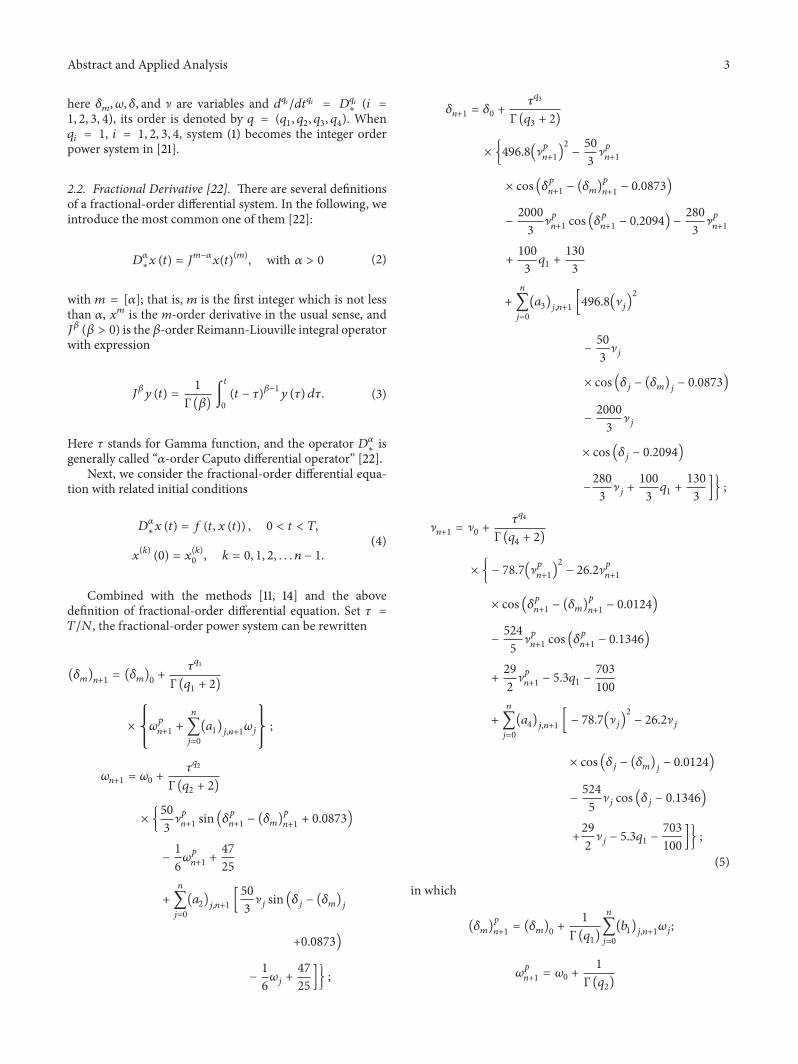
integer order, the 3D trajectory in the power system is shownin Figure 1. The related bifurcation diagram of the parameter𝑄1is shown in Figure 1, and the largest Lyapunov exponent

diagram is shown in Figure 2.

3.2. Dynamic Analysis of the Fractional-Order System. Nextwe correspond to discuss the fractional-order power system.The fractional orders 𝑞

𝑖(𝑖 = 1, 2, 3, 4) are equal and fixed

with at some value which is from 0 to 1. On the basis ofSection 2, first we find that the range of parameter is changingalong with the changing of fractional order. When we let𝑞𝑖= 0.99 (𝑖 = 1, 2, 3, 4) be an example while the parameter

𝑄1is changed from 0 to 11.4 [21]. For a step size in 𝑄

1is

0.01, we clearly got the range of 𝑄1∈ (6, 11.4) in which the

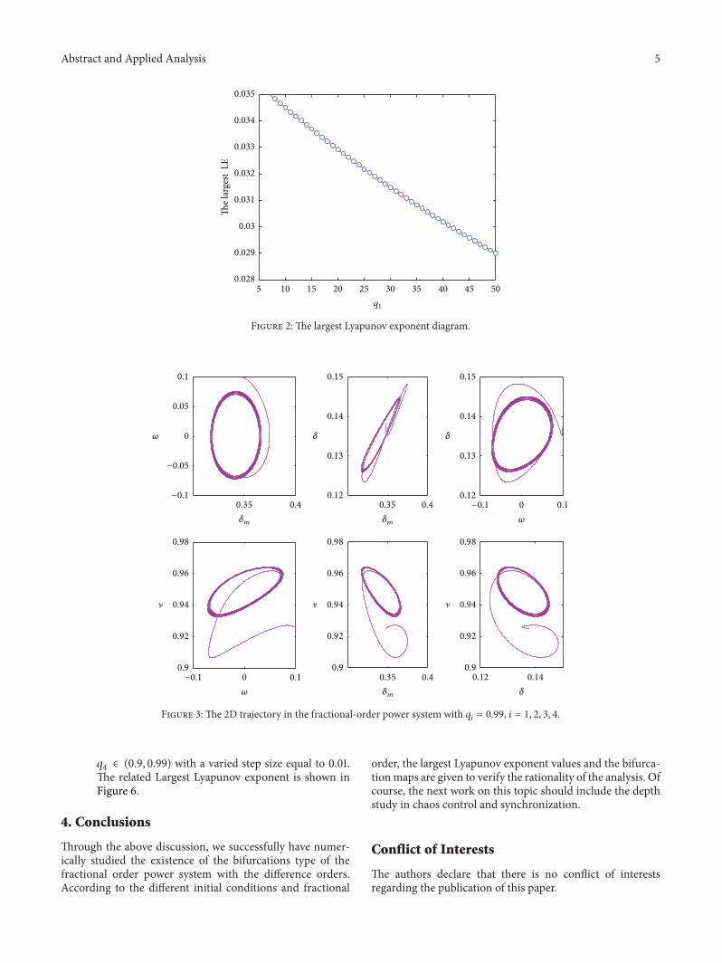
solutions of the fractional-order power system are bounded.We take𝑄

1= 11.37 as an example, the 2D trajectory is shown

in Figure 3 which clearly finds the difference between twoorders 0.99 and 1. The difference is that the former generateschaotic phenomena and the later happens that after a periodof offloading shock of system voltage, ultimately stabilize ata certain value, corresponding to the equilibrium point isasymptotically stable focus. Further, we let 𝑞

𝑖= 0.9 (𝑖 =

1, 2, 3, 4); we clearly got the range of 𝑄1∈ (1, 5.9). The 2D

trajectory is shown in Figure 4 in which𝑄1= 1 and𝑄

1= 5.9.

3.3. Dynamic Analysis with Different Order

(1) Fix 𝑞2= 𝑞3= 𝑞4= 1, 𝑄

1= 11, and let 𝑞

1vary. We

calculate numerically the fractional-power system for𝑞1∈ (0.9, 0.99) with a varied step size equal to 0.01.

The related Largest Lyapunov exponent is shown inFigure 5.

(2) Fix 𝑞1= 𝑞3= 𝑞4= 1, 𝑄

1= 11, and let 𝑞

2vary. We



(3) Fix 𝑞1= 𝑞2= 𝑞4= 1, 𝑄

1= 11, and let 𝑞

3vary. We



(4) Fix 𝑞1= 𝑞2= 𝑞3= 1, 𝑄

1= 11, and let 𝑞

4vary. We

calculate numerically the fractional-power system for


5 10 15 20 25 30 35 40 45 500.028

0.029

0.03

0.031

0.032

0.033

0.034

0.035

The l

arge

st L

E

q1

Figure 2: The largest Lyapunov exponent diagram.

0.35 0.4−0.1

−0.05

0

0.05

0.1

𝜔

𝛿m

0.35 0.40.12

0.13

0.14

0.15

𝛿m

𝛿

−0.1 0 0.10.12

0.13

0.14

0.15

𝜔

𝛿

−0.1 0 0.10.9

0.92

0.94

0.96

0.98

𝜔

�

0.35 0.40.9

0.92

0.94

0.96

0.98

𝛿m

�

0.12 0.140.9

0.92

0.94

0.96

0.98

𝛿

�

Figure 3: The 2D trajectory in the fractional-order power system with 𝑞𝑖= 0.99, 𝑖 = 1, 2, 3, 4.

𝑞4∈ (0.9, 0.99) with a varied step size equal to 0.01.


4. Conclusions

Through the above discussion, we successfully have numer-ically studied the existence of the bifurcations type of thefractional order power system with the difference orders.According to the different initial conditions and fractional

order, the largest Lyapunov exponent values and the bifurca-tionmaps are given to verify the rationality of the analysis. Ofcourse, the next work on this topic should include the depthstudy in chaos control and synchronization.

Conflict of Interests

The authors declare that there is no conflict of interestsregarding the publication of this paper.


0 1 2−0.5

0

0.5

1

1.5

𝜔

𝛿m

0 0.5 10

5

10

𝛿m

𝛿

20 0.5 1 1.5

4

6

8

10

𝜔

𝛿

0 0.5 1 1.5−0.5

0

0.5

1

𝜔

�

0 0.5 1 1.5−0.5

0

0.5

1

𝛿m

�

0 5 10−0.5

0

0.5

1

𝛿

�

(a)

0 0.5 1−1

0

1

2

𝜔

𝛿m

0.4 0.6 0.89

9.5

10

𝛿m

𝛿

−1 0 1 29

9.5

10

𝜔

𝛿

−1 0 1−0.8

−0.6

−0.4

−0.2

0

𝜔

�

0.5 1−1

−0.8

−0.6

−0.4

−0.2

0

𝛿m

�

9 9.5 10−0.7

−0.6

−0.5

−0.4

−0.3

𝛿

�

(b)

Figure 4: The 2D trajectory in the fractional-order power system with 𝑞𝑖= 0.9, 𝑖 = 1, 2, 3, 4. (a) 𝑄

1= 1; (b) 𝑄

1= 5.9.


0.9 0.92 0.94 0.96 0.98 10.009

0.01

0.011

0.012

Fractional order q1

The largest Lyapunov exponent

(a)

0.9 0.91 0.92 0.93 0.94 0.95 0.96 0.97 0.98 0.99−0.025

−0.02

−0.015

−0.01

−0.005

0

0.005

0.01

Fractional order q1


(b)

Figure 5: The Largest Lyapunov Exponent of the fractional-order power system; (a) 𝑞2= 𝑞3= 𝑞4= 1, 𝑞

1= 0.99, and (b) 𝑞

1= 𝑞3= 𝑞4= 1,

𝑞2= 0.99.

0.9 0.91 0.92 0.93 0.94 0.95 0.96 0.97 0.98 0.990.075

0.076

0.077

0.078The largest Lyapunov exponent

Fractional order q3

(a)


0.9 0.92 0.94 0.96 0.98 10

0.004

0.008

0.012

0.016

Fractional order q4

(b)

Figure 6: The Largest Lyapunov Exponent of the fractional-order power system; (a) 𝑞2= 𝑞1= 𝑞4= 1, 𝑞

3= 0.99, and (b) 𝑞

2= 𝑞3= 𝑞1= 1,

𝑞4= 0.99.

Acknowledgment

The present work was partially supported by the NationalNatural Science Foundation of China under Grant no.61273128.

References

[1] P. Arena, R. Caponetto, L. Fortuna, and D. Porto, “Chaos in afractional order duffing system,” in Proceedings of the ECCTD,pp. 1259–1262, Budapest, Hungary, 1997.

[2] Z.-M. Ge and C.-Y. Ou, “Chaos in a fractional order modifiedDuffing system,” Chaos, Solitons and Fractals, vol. 34, no. 2, pp.262–291, 2007.

[3] W. Ahmad, R. El-khazali, and A. S. Elwakil, “Fractional-orderWien-bridge oscillator,” Electronics Letters, vol. 37, no. 18, pp.1110–1112, 2001.

[4] W. M. Ahmad and J. C. Sprott, “Chaos in fractional-orderautonomous nonlinear systems,” Chaos, Solitons and Fractals,vol. 16, no. 2, pp. 339–351, 2003.

[5] W.M.Ahmad andA.M.Harb, “On nonlinear control design forautonomous chaotic systems of integer and fractional orders,”Chaos, Solitons and Fractals, vol. 18, no. 4, pp. 693–701, 2003.

[6] X. Zhang, L. Liu, and Y. Wu, “The uniqueness of positivesolution for a singular fractional differential system involvingderivatives,” Communications in Nonlinear Science and Numer-ical Simulation, vol. 18, no. 6, pp. 1400–1409, 2013.


[7] X. Zhang, L. Liu, and Y. Wu, “Multiple positive solutionsof a singular fractional differential equation with negativelyperturbed term,” Mathematical and Computer Modelling, vol.55, no. 3-4, pp. 1263–1274, 2012.

[8] X. Zhang, L. Liu, and Y. Wu, “The eigenvalue problem for asingular higher order fractional differential equation involvingfractional derivatives,” Applied Mathematics and Computation,vol. 218, no. 17, pp. 8526–8536, 2012.

[9] X. Zhang, L. Liu, and Y.Wu, “Existence results for multiple pos-itive solutions of nonlinear higher order perturbed fractionaldifferential equations with derivatives,” Applied Mathematicsand Computation, vol. 219, no. 4, pp. 1420–1433, 2012.

[10] H. H. Sun, A. A. Abdelwahab, and B. Onaral, “Linear approx-imation of transfer function with a pole of fractional power,”IEEE Transactions on Automatic Control, vol. 29, no. 5, pp. 441–444, 1984.

[11] K. Diethelm and N. J. Ford, “Analysis of fractional differentialequations,” Journal of Mathematical Analysis and Applications,vol. 265, no. 2, pp. 229–248, 2002.

[12] M. S. Tavazoei and M. Haeri, “Unreliability of frequency-domain approximation in recognising chaos in fractional-ordersystems,” IET Signal Processing, vol. 1, no. 4, pp. 171–181, 2007.

[13] M. S. Tavazoei andM. Haeri, “Limitations of frequency domainapproximation for detecting chaos in fractional order systems,”Nonlinear Analysis: Theory, Methods & Applications, vol. 69, no.4, pp. 1299–1320, 2008.

[14] K. Diethelm, N. J. Ford, and A. D. Freed, “A predictor-correctorapproach for the numerical solution of fractional differentialequations,”Nonlinear Dynamics, vol. 29, no. 1-4, pp. 3–22, 2002.

[15] C. Li and G. Peng, “Chaos in Chen’s system with a fractionalorder,” Chaos, Solitons & Fractals, vol. 22, no. 2, pp. 443–450,2004.

[16] M. S. Tavazoei andM. Haeri, “Chaotic attractors in incommen-surate fractional order systems,” Physica D, vol. 237, no. 20, pp.2628–2637, 2008.

[17] K. Sun, X. Wang, and J. C. Sprott, “Bifurcations and chaos infractional-order simplified Lorenz system,” International Jour-nal of Bifurcation andChaos inApplied Sciences andEngineering,vol. 20, no. 4, pp. 1209–1219, 2010.

[18] I.-D. Chiang, C.-W. Liu, P. P. Varaiya, F. F. Wu, andM. G. Lauby,“Chaos in a simple power system,” IEEE Transactions on PowerSystems, vol. 8, no. 4, pp. 1407–1409, 1993.

[19] Z. Jing, D. Xu, Y. Chang, and L. Chen, “Bifurcations, chaos, andsystem collapse in a three node power system,” InternationalJournal of Electrical Power and Energy System, vol. 25, no. 6, pp.443–461, 2003.

[20] S. Grillo, S. Massucco, A. Morini, A. Pitto, and F. Silvestre,“Bifurcation analysis and Chaos detection in power systems,”in Proceedings of the 43rd International Universities PowerEngineering Conference (UPECn ’08), pp. 1–6, September 2008.

[21] H.-D. Chiang, I. Dobson, R. J.Thomas, J. S.Thorp, and L. Fekih-Ahmed, “On voltage collapse in electric power systems,” IEEETransactions on Power Systems, vol. 5, no. 2, pp. 601–611, 1990.

[22] M. Caputo, “Linear models of dissipation whose 𝑄 is almostfrequency Independent-II.,” Geophysical Journal of the RoyalAstronomical Society, vol. 13, pp. 529–539, 1967.

Submit your manuscripts athttp://www.hindawi.com

Hindawi Publishing Corporationhttp://www.hindawi.com Volume 2014

MathematicsJournal of


Mathematical Problems in Engineering

Hindawi Publishing Corporationhttp://www.hindawi.com

Differential EquationsInternational Journal of

Volume 2014

Applied MathematicsJournal of


Probability and StatisticsHindawi Publishing Corporationhttp://www.hindawi.com Volume 2014

Journal of


Mathematical PhysicsAdvances in

Complex AnalysisJournal of


OptimizationJournal of


CombinatoricsHindawi Publishing Corporationhttp://www.hindawi.com Volume 2014

International Journal of


Operations ResearchAdvances in

Journal of


Function Spaces

Abstract and Applied AnalysisHindawi Publishing Corporationhttp://www.hindawi.com Volume 2014

International Journal of Mathematics and Mathematical Sciences


The Scientific World JournalHindawi Publishing Corporation http://www.hindawi.com Volume 2014


Algebra

Discrete Dynamics in Nature and Society



Decision SciencesAdvances in

Discrete MathematicsJournal of

Hindawi Publishing Corporationhttp://www.hindawi.com

Volume 2014 Hindawi Publishing Corporationhttp://www.hindawi.com Volume 2014

Stochastic AnalysisInternational Journal of

Research Article Dynamic Analysis and Chaos of the 4D ...

Documents

Transcript of Research Article Dynamic Analysis and Chaos of the 4D ...