Research Article An Efficient Family of Traub-Steffensen ...
12
Research Article An Efficient Family of Traub-Steffensen-Type Methods for Solving Systems of Nonlinear Equations Janak Raj Sharma 1 and Puneet Gupta 2 1 Department of Mathematics, Sant Longowal Institute of Engineering and Technology, Longowal, Punjab 148 106, India 2 Department of Mathematics, Government Ranbir College, Sangrur, Punjab 148 001, India Correspondence should be addressed to Janak Raj Sharma; [email protected] Received 6 February 2014; Accepted 11 June 2014; Published 2 July 2014 Academic Editor: Zhangxin Chen Copyright © 2014 J. R. Sharma and P. Gupta. is is an open access article distributed under the Creative Commons Attribution License, which permits unrestricted use, distribution, and reproduction in any medium, provided the original work is properly cited. Based on Traub-Steffensen method, we present a derivative free three-step family of sixth-order methods for solving systems of nonlinear equations. e local convergence order of the family is determined using first-order divided difference operator for functions of several variables and direct computation by Taylor’s expansion. Computational efficiency is discussed, and a comparison between the efficiencies of the proposed techniques with the existing ones is made. Numerical tests are performed to compare the methods of the proposed family with the existing methods and to confirm the theoretical results. It is shown that the new family is especially efficient in solving large systems. 1. Introduction e problem of finding solution of the system of nonlinear equations () = 0, where : → , is an open convex domain in , by iterative methods is an important and challenging task in numerical analysis and many applied scientific branches. One of the basic procedures for solving nonlinear equations is the quadratically convergent Newton method (see [1, 2]): (+1) = () − [ ( () )] −1 ( () ), = 0, 1, 2, . . . , (1) where [ ()] −1 is the inverse of the first Fr´ echet derivative () of the function (). In many practical situations, it is preferable to avoid the calculation of derivative () of the function (). In such situations, it is preferable to use only the computed values of () and to approximate () by employing the values of () at suitable points. For example, a basic derivative free iterative method is the Traub-Steffensen method [3], which also converges quadratically and follows the scheme (+1) = 1,2 ( () )= () − [ () , () ; ] −1 ( () ), (2) where [ () , () ; ] −1 is the inverse of the first-order divided difference [ () , () ; ] of and () = () + ( () ); is an arbitrary nonzero constant. roughout this paper, , is used to denote the th iteration function of convergence order . For =1, the scheme (2) reduces to the well-known Steffensen method [4]. In recent years, many derivative free higher-order meth- ods of great efficiency are developed for solving scalar equation () = 0; see [5–14] and the references therein. For systems of nonlinear equations, however, the construction of efficient higher-order derivative free methods is a difficult task and therefore not many such methods can be found in the literature. Recently, based on Steffensen’s scheme, that is, when =1 in (2), a family of seventh-order methods has been proposed in [13]. Some important members of this family, as shown in [13], are given as follows: () = 1,2 ( () ), () = 1,4 ( () , () ) = () − ([ () , () ; ] + [ () , () ; ] Hindawi Publishing Corporation Advances in Numerical Analysis Volume 2014, Article ID 152187, 11 pages http://dx.doi.org/10.1155/2014/152187
Transcript of Research Article An Efficient Family of Traub-Steffensen ...
Research ArticleAn Efficient Family of Traub-Steffensen-Type Methods forSolving Systems of Nonlinear Equations
Janak Raj Sharma1 and Puneet Gupta2
1 Department of Mathematics Sant Longowal Institute of Engineering and Technology Longowal Punjab 148 106 India2Department of Mathematics Government Ranbir College Sangrur Punjab 148 001 India
Correspondence should be addressed to Janak Raj Sharma jrshirayahoocoin
Received 6 February 2014 Accepted 11 June 2014 Published 2 July 2014
Academic Editor Zhangxin Chen
Copyright copy 2014 J R Sharma and P Gupta This is an open access article distributed under the Creative Commons AttributionLicense which permits unrestricted use distribution and reproduction in any medium provided the original work is properlycited
Based on Traub-Steffensen method we present a derivative free three-step family of sixth-order methods for solving systemsof nonlinear equations The local convergence order of the family is determined using first-order divided difference operatorfor functions of several variables and direct computation by Taylorrsquos expansion Computational efficiency is discussed and acomparison between the efficiencies of the proposed techniques with the existing ones is made Numerical tests are performedto compare the methods of the proposed family with the existing methods and to confirm the theoretical results It is shown thatthe new family is especially efficient in solving large systems
1 Introduction
The problem of finding solution of the system of nonlinearequations 119865(119909) = 0 where 119865 119863 rarr 119863 119863 is an openconvex domain in 119877
119899 by iterative methods is an importantand challenging task in numerical analysis and many appliedscientific branches One of the basic procedures for solvingnonlinear equations is the quadratically convergent Newtonmethod (see [1 2])
119909(119896+1)
= 119909(119896)
minus [1198651015840
(119909(119896)
)]minus1
119865 (119909(119896)
) 119896 = 0 1 2 (1)
where [1198651015840(119909)]minus1 is the inverse of the first Frechet derivative1198651015840
(119909) of the function 119865(119909)In many practical situations it is preferable to avoid the
calculation of derivative 1198651015840(119909) of the function 119865(119909) In suchsituations it is preferable to use only the computed values of119865(119909) and to approximate 1198651015840(119909) by employing the values of119865(119909) at suitable points For example a basic derivative freeiterative method is the Traub-Steffensen method [3] whichalso converges quadratically and follows the scheme
119909(119896+1)
= 11986612(119909(119896)
) = 119909(119896)
minus [119908(119896)
119909(119896)
119865]minus1
119865 (119909(119896)
) (2)
where [119908(119896) 119909(119896) 119865]minus1 is the inverse of the first-order divideddifference [119908(119896) 119909(119896) 119865] of 119865 and 119908
(119896)
= 119909(119896)
+ 120574119865(119909(119896)
)120574 isan arbitrary nonzero constant Throughout this paper 119866
119894119901
is used to denote the 119894th iteration function of convergenceorder 119901 For 120574 = 1 the scheme (2) reduces to the well-knownSteffensen method [4]
In recent years many derivative free higher-order meth-ods of great efficiency are developed for solving scalarequation 119891(119909) = 0 see [5ndash14] and the references therein Forsystems of nonlinear equations however the construction ofefficient higher-order derivative free methods is a difficulttask and therefore not many such methods can be found inthe literature Recently based on Steffensenrsquos scheme thatis when 120574 = 1 in (2) a family of seventh-order methodshas been proposed in [13] Some important members of thisfamily as shown in [13] are given as follows
119910(119896)
= 11986612(119909(119896)
)
119911(119896)
= 11986614(119909(119896)
119910(119896)
)
= 119910(119896)
minus ([119910(119896)
119909(119896)
119865] + [119910(119896)
119908(119896)
119865]
Hindawi Publishing CorporationAdvances in Numerical AnalysisVolume 2014 Article ID 152187 11 pageshttpdxdoiorg1011552014152187
2 Advances in Numerical Analysis
minus [119908(119896)
119909(119896)
119865])minus1
119865 (119910(119896)
)
119909(119896+1)
= 11986617(119909(119896)
119910(119896)
119911(119896)
)
= 119911(119896)
minus ([119911(119896)
119909(119896)
119865] + [119911(119896)
119910(119896)
119865]
minus [119910(119896)
119909(119896)
119865])minus1
119865 (119911(119896)
)
(3)
119910(119896)
= 11986612(119909(119896)
)
119911(119896)
= 11986624(119909(119896)
119910(119896)
)
= 119910(119896)
minus [119910(119896)
119909(119896)
119865]minus1
times ([119910(119896)
119909(119896)
119865] minus [119910(119896)
119908(119896)
119865]
+ [119908(119896)
119909(119896)
119865]) [119910(119896)
119909(119896)
119865]minus1
119865 (119910(119896)
)
119909(119896+1)
= 11986627(119909(119896)
119910(119896)
119911(119896)
)
= 119911(119896)
minus ([119911(119896)
119909(119896)
119865] + [119911(119896)
119910(119896)
119865]
minus [119910(119896)
119909(119896)
119865])minus1
119865 (119911(119896)
)
(4)
Per iteration bothmethods use four functions five first-orderdivided differences and three matrix inversions The notablefeature of these algorithms is their simple design whichmakes them easily implemented to solve systems of nonlinearequations Here the fourth-order method 119866
14(119909(119896)
119910(119896)
) isthe generalization of the method proposed by Ren et al in[5] and 119866
24(119909(119896)
119910(119896)
) is the generalization of the method byLiu et al [6]
In this paper our aim is to develop derivative free iterativemethods thatmay satisfy the basic requirements of generatingquality numerical algorithms that is the algorithms with(i) high convergence speed (ii) minimum computationalcost and (iii) simple design In this way we here propose aderivative free family of sixth-order methods The scheme iscomposed of three steps of which the first two steps consistof any derivative free fourth-order method with the baseas the Traub-Steffensen iteration (2) whereas the third stepis weighted Traub-Steffensen iteration The algorithm of thepresent contribution is as simple as the methods (3) and(4) but with an additional advantage that it possesses highcomputational efficiency especially when applied for solvinglarge systems of equations
The rest of the paper is summarized as followsThe sixth-order scheme with its convergence analysis is presented inSection 2 In Section 3 the computational efficiency of newmethods is discussed and is compared with the methodswhich lie in the same category Various numerical examplesare considered in Section 4 to show the consistent conver-gence behavior of the methods and to verify the theoreticalresults Section 5 contains the concluding remarks
2 The Method and Its Convergence
Based on the above considerations of a quality numericalalgorithm we begin with the following three-step iterationscheme
119910(119896)
= 11986612(119909(119896)
)
119911(119896)
= 1198664(119909(119896)
119910(119896)
)
119909(119896+1)
= 1198666(119909(119896)
119910(119896)
119911(119896)
)
= 119911(119896)
minus (119886119868 + [119908(119896)
119909(119896)
119865]minus1
times (119887 [119910(119896)
119909(119896)
119865] + 119888 [119910(119896)
119908(119896)
119865]) )
times [119908(119896)
119909(119896)
119865]minus1
119865 (119911(119896)
)
(5)
where 1198664(119909(119896)
119910(119896)
) denotes any derivative free fourth-orderscheme and 119886 119887 119888 are some parameters to be determined
In order to find the convergence order of scheme (5)we first define divided difference operator for multivariablefunction 119865 (see [15]) The divided difference operator of 119865 isa mapping [sdot sdot 119865] 119863 times 119863 sub 119877
119899
times 119877119899
rarr 119871(119877119899
) defined by
[119909 + ℎ 119909 119865] = int
1
0
1198651015840
(119909 + 119905ℎ) 119889119905 forall119909 ℎ isin 119877119899
(6)
Expanding 1198651015840(119909 + 119905ℎ) in Taylor series at the point 119909 and thenintegrating we have
[119909 + ℎ 119909 119865] = int
1
0
1198651015840
(119909 + 119905ℎ) 119889119905
= 1198651015840
(119909) +1
211986510158401015840
(119909) ℎ +1
6119865101584010158401015840
(119909) ℎ2
+ 119874 (ℎ3
)
(7)
where ℎ119894 = (ℎ ℎ 119894 ℎ) ℎ isin 119877119899
Let 119890(119896) = 119909(119896)
minus 120572 Assuming that Γ = [1198651015840
(120572)]minus1 exists
and then developing 119865(119909(119896)) and its first three derivatives in aneighborhood of 120572 we have
119865 (119909(119896)
) = 1198651015840
(120572) (119890(119896)
+ 1198602(119890(119896)
)2
+ 1198603(119890(119896)
)3
+ 1198604(119890(119896)
)4
+ 1198605(119890(119896)
)5
+ 119874((119890(119896)
)6
))
(8)
1198651015840
(119909(119896)
) = 1198651015840
(120572) (119868 + 21198602119890(119896)
+ 31198603(119890(119896)
)2
+ 41198604(119890(119896)
)3
+ 51198605(119890(119896)
)4
+ 119874((119890(119896)
)5
))
(9)
Advances in Numerical Analysis 3
11986510158401015840
(119909(119896)
) = 1198651015840
(120572) (21198602+ 61198603119890(119896)
+ 121198604(119890(119896)
)2
+ 201198605(119890(119896)
)3
+ 119874((119890(119896)
)4
))
(10)
119865101584010158401015840
(119909(119896)
) = 1198651015840
(120572) (61198603+ 24119860
4119890(119896)
+ 601198605(119890(119896)
)2
+ 119874((119890(119896)
)3
))
(11)
where 119860119894= (1119894)Γ119865
(119894)
(120572) isin 119871119894(119877119899
119877119899
) and (119890(119896)
)119894
= (119890(119896)
119890(119896)
119894 119890(119896)
) 119890(119896)
isin 119877119899 119860119894are symmetric operators that are
used later onWe can now analyze behavior of the scheme (5) through
the following theorem
Theorem 1 Let the function 119865 119863 sub 119877119899
rarr 119877119899 be sufficiently
differentiable in an open neighborhood 119863 of its zero 120572 and1198664(119909(119896)
119910(119896)
) is a fourth-order iteration functionwhich satisfies
119890(119896)
119911= 119911(119896)
minus 120572 = 1198610(119890(119896)
)4
+ 119874((119890(119896)
)5
) (12)
where 1198610isin 1198714(119877119899
119877119899
) and 119890(119896)
= 119909(119896)
minus 120572 If an initialapproximation 119909(0) is sufficiently close to 120572 then the local orderof convergence of method (5) is at least 6 provided 119886 = 3119887 = minus1 and 119888 = minus1
Proof Let 119890(119896)119908
= 119908(119896)
minus 120572 = 119909(119896)
+ 120574119865(119909(119896)
) minus 120572 Then using(8) it follows that
119890(119896)
119908= (119868 + 120574119865
1015840
(120572)) 119890(119896)
+ 1205741198651015840
(120572) 1198602(119890(119896)
)2
+ 1205741198651015840
(120572) 1198603(119890(119896)
)3
+ 119874((119890(119896)
)4
)
(13)
Employing (7) for 119909 + ℎ = 119908(119896) 119909 = 119909
(119896) and ℎ = 119890(119896)
119908minus 119890(119896)
and then using (9)ndash(11) we write
[119908(119896)
119909(119896)
119865] = 1198651015840
(120572)
times [119868 + 1198602(119890(119896)
119908+ 119890(119896)
)
+ 1198603((119890(119896)
119908)2
+ (119890(119896)
)2
+ 119890(119896)
119908119890(119896)
)
+ 1198604((119890(119896)
119908)3
+ (119890(119896)
)3
+ (119890(119896)
119908)2
119890(119896)
+ 119890(119896)
119908(119890(119896)
)2
)
+ 119874((119890(119896)
)4
)]
(14)
Expanding in the formal power developments the inverse ofpreceding operator can be written as
[119908(119896)
119909(119896)
119865]minus1
= [119868 minus 1198602(119890(119896)
119908+ 119890(119896)
) + (1198602
2minus 1198603)
times ((119890(119896)
119908)2
+ (119890(119896)
)2
)
+ (21198602
2minus 1198603) 119890(119896)
119908119890(119896)
minus (1198603
2minus 11986031198602minus 11986021198603+ 1198604)
times ((119890(119896)
119908)3
+ (119890(119896)
)3
)
minus (31198603
2minus 211986031198602minus 211986021198603+ 1198604)
times ((119890(119896)
119908)2
119890(119896)
+ 119890(119896)
119908(119890(119896)
)2
)
+ 119874((119890(119896)
)4
)] Γ
(15)
Using (8) and (15) to the required terms in the first step of (5)we find that
119890(119896)
119910= 119910(119896)
minus 120572
= 1198602119890(119896)
119908119890(119896)
minus (1198602
2minus 1198603)
times ((119890(119896)
119908)2
119890(119896)
+ 119890(119896)
119908(119890(119896)
)2
) + 119874((119890(119896)
)4
)
(16)
Equation (7) for 119909 + ℎ = 119910(119896) 119909 = 119909
(119896) and ℎ = 119890(119896)
119910minus 119890(119896)
yields
[119910(119896)
119909(119896)
119865] = 1198651015840
(120572) [119868 + 1198602(119890(119896)
119910+ 119890(119896)
)
+ 1198603(119890(119896)
119910119890(119896)
+ (119890(119896)
)2
)
+ 1198604(119890(119896)
)3
+ 119874((119890(119896)
)4
)]
(17)
Similarly substituting 119909+ℎ = 119910(119896) 119909 = 119908
(119896) and ℎ = 119890(119896)
119910minus119890(119896)
119908
in (7) we obtain
[119910(119896)
119908(119896)
119865] = 1198651015840
(120572) [119868 + 1198602(119890(119896)
119910+ 119890(119896)
119908)
+ 1198603(119890(119896)
119910119890(119896)
119908+ (119890(119896)
119908)2
)
+ 1198604(119890(119896)
w )3
+ 119874 ((119890(119896)
)4
)]
(18)
4 Advances in Numerical Analysis
Then using (15) (17) and (18) to the required terms we findthat
119886119868 + [119908(119896)
119909(119896)
119865]minus1
(119887 [119910(119896)
119909(119896)
119865] + 119888 [119910(119896)
119908(119896)
119865])
= (119886 + 119887 + 119888) 119868 minus 1198602(119887119890(119896)
119908+ 119888119890(119896)
)
+ (1198602
2minus 1198603) (119887(119890
(119896)
119908)2
+ 119888(119890(119896)
)2
)
+ (119887 + 119888) (1198602
2minus 1198603) 119890(119896)
119908119890(119896)
+ (119887 + 119888) 1198602119890(119896)
119910
+ 119874((119890(119896)
)3
)
(19)
Postmultiplying (19) by [119908(119896) 119909(119896) 119865]minus1 and simplifying
120579 = (119886119868 + [119908(119896)
119909(119896)
119865]minus1
times (119887 [119910(119896)
119909(119896)
119865] + 119888 [119910(119896)
119908(119896)
119865]) )
times [119908(119896)
119909(119896)
119865]minus1
= [ (119886 + 119887 + 119888) 119868 minus (119886 + 2119887 + 119888) 1198602119890(119896)
119908
minus (119886 + 119887 + 2119888) 1198602119890(119896)
+ ((119886 + 3119887 + 119888) 1198602
2minus (119886 + 2119887 + 119888) 119860
3) (119890(119896)
119908)2
+ ((119886 + 119887 + 3119888) 1198602
2minus (119886 + 119887 + 2119888) 119860
3) (119890(119896)
)2
+ (119886 + 2 (119887 + 119888)) (21198602
2minus 1198603) 119890(119896)
119908119890(119896)
+ (119887 + 119888) 1198602119890(119896)
119910+ 119874((119890
(119896)
)3
)] Γ
(20)
Taylor series of 119865(119911(119896)) about 120572 yields
119865 (119911(119896)
) = 1198651015840
(120572) [119890(119896)
119911+ 1198602(119890(119896)
119911)2
+ 119874((119890(119896)
119911)3
)] (21)
Then using (20) and (21) in the third step of (5) we obtainthe error equation as
119890(119896+1)
= 119890(119896)
119911minus 120579 119865
1015840
(120572) [119890(119896)
119911+ 119874((119890
(119896)
119911)2
)]
= minus (119886 + 119887 + 119888 minus 1) 119890(119896)
119911+ (119886 + 2119887 + 119888) 119860
2119890(119896)
119908119890(119896)
119911
+ (119886 + 119887 + 2119888) 1198602119890(119896)
119911119890(119896)
minus ((119886 + 3119887 + 119888) 1198602
2minus (119886 + 2119887 + 119888) 119860
3) (119890(119896)
119908)2
119890(119896)
119911
minus ((119886 + 119887 + 3119888) 1198602
2minus (119886 + 119887 + 2119888) 119860
3)
times 119890(119896)
119911(119890(119896)
)2
minus (119886 + 2 (119887 + 119888))
times (21198602
2minus 1198603) 119890(119896)
119908119890(119896)
119911119890(119896)
minus (119887 + 119888) 1198602119890(119896)
119910119890(119896)
119911+ 119874((119890
(119896)
)7
)
(22)
In order to find 119886 119887 and 119888 it will be sufficient to equate thefactors 119886 + 119887 + 119888 minus 1 119886 + 2119887 + 119888 and 119886 + 119887 + 2119888 to 0 and thensolving the resulting system of equations
119886 + 119887 + 119888 = 1 119886 + 2119887 + 119888 = 0 119886 + 119887 + 2119888 = 0 (23)
we obtain 119886 = 3 119887 = minus1 and 119888 = minus1Thus for this set of values the above error equation
reduces to
119890(119896+1)
= 1198602
2(119890(119896)
119908+ 119890(119896)
)2
119890(119896)
119911+ 21198602119890(119896)
119910119890(119896)
119911
minus 1198603119890(119896)
119908119890(119896)
119911119890(119896)
+ 119874((119890(119896)
)7
)
= 1198610((119868 + 120574119865
1015840
(120572)) (61198602
2minus 1198603)
+1205742
(1198651015840
(120572))2
1198602
2) (119890(119896)
)6
+ 119874((119890(119896)
)7
)
(24)
which shows the sixth order of convergence and hence theresult follows
Finally the sixth-order family of methods is expressed by
119910(119896)
= 11986612(119909(119896)
)
119911(119896)
= 1198664(119909(119896)
119910(119896)
)
119909(119896+1)
= 1198666(119909(119896)
119910(119896)
119911(119896)
)
= 119911(119896)
minusM (119909(119896)
119908(119896)
119910(119896)
) 119865 (119911(119896)
)
(25)
wherein
M (119909(119896)
119908(119896)
119910(119896)
) = (3119868 minus [119908(119896)
119909(119896)
119865]minus1
([119910(119896)
119909(119896)
119865]
+ [119910(119896)
119908(119896)
119865])) [119908(119896)
119909(119896)
119865]minus1
(26)
Thus the scheme (25) defines a new three-step family ofderivative free sixth-order methods with the first two steps asany fourth-order scheme whose base is the Traub-Steffensenmethod (3) Some simple members of this family are asfollows
Method-IThe first method which is denoted by11986616 is given
by
119910(119896)
= 11986612(119909(119896)
)
119911(119896)
= 11986614(119909(119896)
119910(119896)
)
119909(119896+1)
= 119911(119896)
minusM (119909(119896)
119908(119896)
119910(119896)
) 119865 (119911(119896)
)
(27)
Advances in Numerical Analysis 5
where 11986614(119909(119896)
119910(119896)
) is the fourth-order method as givenin the formula (3) It is clear that this formula uses fourfunctions three first-order divided differences and twomatrix inversions per iteration
Method-II The second method that we denote by 11986626 is
given as
119910(119896)
= 11986612(119909(119896)
)
119911(119896)
= 11986624(119909(119896)
119910(119896)
)
119909(119896+1)
= 119911(119896)
minusM (119909(119896)
119908(119896)
119910(119896)
) 119865 (119911(119896)
)
(28)
where 11986624(119909(119896)
119910(119896)
) is the fourth-order method shown in(4) This method also requires the same evaluations as in theabove method
3 Computational Efficiency
Here we estimate the computational efficiency of the pro-posed methods and compare it with the existing methodsTo do this we will make use of efficiency index accordingto which the efficiency of an iterative method is given by119864 = 120588
1119862 where 120588 is the order of convergence and 119862
is the computational cost per iteration For a system of 119899nonlinear equations in 119899 unknowns the computational costper iteration is given by (see [16])
119862 (120583 119899 119897) = 1198750(119899) 120583 + 119875 (119899 119897) (29)
Here 1198750(119899) denotes the number of evaluations of scalar
functions used in the evaluation of 119865 and [119909 119910 119865] and 119875(119899 119897)denotes the number of products needed per iteration Thedivided difference [119909 119910 119865] of 119865 is an 119899 times 119899 matrix withelements given as (see [17 18])
[119910 119909 119865]119894119895= (119891119894(1199101 119910
119895minus1 119910119895 119909119895+1
119909119899)
minus 119891119894(1199101 119910
119895minus1 119909119895 119909119895+1
119909119899)
+ 119891119894(1199091 119909
119895minus1 119910119895 119910119895+1
119910119899)
minus 119891119894(1199091 119909
119895minus1 119909119895 119910119895+1
119910119899))
times ((2 (119910119895minus 119909119895)))minus1
1 ⩽ 119894 119895 ⩽ 119899
(30)
In order to express the value of119862(120583 119899 119897) in terms of productsa ratio 120583 gt 0 between products and evaluations of scalarfunctions and a ratio 119897 ⩾ 1 between products and quotientsare required
To compute 119865 in any iterative function we evaluate119899 scalar functions (119891
1 1198912 119891
119899) and if we compute a
divided difference [119909 119910 119865] then we evaluate 2119899(119899 minus 1) scalarfunctions where 119865(119909) and 119865(119910) are computed separatelyWe must add 119899
2 quotients from any divided difference 1198992products for multiplication of a matrix with a vector or ofa matrix by a scalar and 119899 products for multiplication ofa vector by a scalar In order to compute an inverse linear
operator we solve a linear system where we have 119899(119899 minus
1)(2119899 minus 1)6 products and 119899(119899 minus 1)2 quotients in the LUdecomposition and 119899(119899 minus 1) products and 119899 quotients in theresolution of two triangular linear systems
The computational efficiency of the present sixth-ordermethods 119866
16and 119866
26is compared with the existing fourth-
order methods 11986614
and 11986624
and with the seventh-ordermethods 119866
17and 119866
27 In addition we also compare the
present methods with each other Let us denote efficiencyindices of 119866
119894119901by 119864119894119901
and computational cost by 119862119894119901 Then
taking into account the above and previous considerationswe have
11986214
= (61198992
minus 3119899) 120583 +119899
3(21198992
+ 3119899 minus 5 + 3119897 (4119899 + 1))
11986414
= 4111986214
(31)
11986224
= (61198992
minus 3119899) 120583 +119899
3(21198992
+ 9119899 minus 8 + 3119897 (4119899 + 2))
11986424
= 4111986224
(32)
11986216
= (61198992
minus 2119899) 120583 +119899
3(21198992
+ 12119899 minus 8 + 3119897 (4119899 + 3))
11986416
= 6111986216
(33)
11986226
= (61198992
minus 2119899) 120583 +119899
3(21198992
+ 18119899 minus 11 + 12119897 (119899 + 1))
11986426
= 6111986226
(34)
11986217
= (101198992
minus 6119899) 120583 +119899
2(21198992
+ 3119899 minus 5 + 119897 (13119899 + 3))
11986417
= 7111986217
(35)
11986227
= (101198992
minus 6119899) 120583 +119899
2(21198992
+ 7119899 minus 7 + 119897 (13119899 + 5))
11986427
= 7111986227
(36)
31 Comparison between Efficiencies To compare the compu-tational efficiencies of the iterative methods say 119866
119894119901against
119866119895119902 we consider the ratio
119877119894119901119895119902
=
log119864119894119901
log119864119895119902
=
119862119895119902
log (119901)119862119894119901log (119902)
(37)
It is clear that if 119877119894119901119895119902
gt 1 the iterative method 119866119894119901
is moreefficient than 119866
119895119902
11986614
versus 11986616
Case For this case the ratio (37) is given by
1198771614
=log 6log 4
21198992
+ 119899 (18120583 + 12119897 + 3) minus 9120583 + 3119897 minus 5
21198992 + 119899 (18120583 + 12119897 + 12) minus 6120583 + 9119897 minus 8
(38)
6 Advances in Numerical Analysis
which shows that 1198771614
gt 1 for 120583 gt 0 119897 ⩾ 1 and 119899 ⩾ 9 Thuswe have 119864
16gt 11986414
for 120583 gt 0 119897 ⩾ 1 and 119899 ⩾ 9
11986624
versus 11986616
Case In this case the ratio (37) takes thefollowing form
1198771624
=log 6log 4
21198992
+ 119899 (18120583 + 12119897 + 9) minus 9120583 + 6119897 minus 8
21198992 + 119899 (18120583 + 12119897 + 12) minus 6120583 + 9119897 minus 8 (39)
In this case it is easy to prove that 1198771624
gt 1 for 120583 gt 0 119897 ⩾ 1and 119899 ⩾ 2 which implies that 119864
16gt 11986424
11986614
versus 11986626
CaseThe ratio (37) yields
1198772614
=log 6log 4
21198992
+ 119899 (18120583 + 12119897 + 3) minus 9120583 + 3119897 minus 5
21198992 + 119899 (18120583 + 12119897 + 18) minus 6120583 + 12119897 minus 11
(40)
which shows that 1198772614
gt 1 for 120583 gt 0 119897 ⩾ 1 and 119899 ⩾ 19Thus we conclude that 119864
26gt 11986414
for 120583 gt 0 119897 ⩾ 1 and119899 ⩾ 19
11986624
versus 11986626
Case In this case the ratio (37) is given by
1198772624
=log 6log 4
21198992
+ 119899 (18120583 + 12119897 + 9) minus 9120583 + 6119897 minus 8
21198992 + 119899 (18120583 + 12119897 + 18) minus 6120583 + 12119897 minus 11
(41)
With the same range of 120583 119897 as in the previous case and 119899 ⩾ 6the ratio 119877
2624gt 1 which implies that 119864
26gt 11986424
11986616
versus 11986626
Case In this case it is enough to comparethe corresponding values of 119862
16and 119862
26from (33) and (34)
Thus we find that 11986416
gt 11986426
for 120583 gt 0 119897 ⩾ 1 and 119899 ⩾ 2
11986616
versus 11986617
Case In this case the ratio (37) is given by
1198771617
=log 6log 7
3 (21198992
+ 119899 (20120583 + 13119897 + 3) minus 12120583 + 3119897 minus 5)
2 (21198992 + 119899 (18120583 + 12119897 + 12) minus 6120583 + 9119897 minus 8)
(42)
It is easy to show that 1198771617
gt 1 for 120583 gt 0 119897 ⩾ 1 and 119899 ⩾ 4which implies that 119864
16gt 11986417
for this range of values of theparameters (120583 119899 119897)
11986616
versus 11986627
Case The ratio (37) is given by
1198771627
=log 6log 7
3 (21198992
+ 119899 (20120583 + 13119897 + 7) minus 12120583 + 5119897 minus 7)
2 (21198992 + 119899 (18120583 + 12119897 + 12) minus 6120583 + 9119897 minus 8)
(43)
With the same range of 120583 119897 as in the previous cases and 119899 ⩾ 2we have 119877
1627gt 1 which implies that 119864
16gt 11986427
11986626
versus 11986617
CaseThe ratio (37) yields
1198772617
=log 6log 7
3 (21198992
+ 119899 (20120583 + 13119897 + 3) minus 12120583 + 3119897 minus 5)
2 (21198992 + 119899 (18120583 + 12119897 + 18) minus 6120583 + 12119897 minus 11)
(44)
which shows that 1198772617
gt 1 for 120583 gt 0 119897 ⩾ 1 and 119899 ⩾ 11 soit follows that 119864
26gt 11986417
11986626
versus 11986627
Case For this case the ratio (37) is given by
1198772627
=log 6log 7
3 (21198992
+ 119899 (20120583 + 13119897 + 7) minus 12120583 + 5119897 minus 7)
2 (21198992 + 119899 (18120583 + 12119897 + 18) minus 6120583 + 12119897 minus 11)
(45)
In this case also it is not difficult to prove that 1198772627
gt 1 for120583 gt 0 119897 ⩾ 1 and 119899 ⩾ 5 which implies that 119864
26gt 11986427
We summarize the above results in the following theorem
Theorem 2 For 120583 gt 0 and 119897 ⩾ 1 we have the following
(i) 11986416
gt 11986414
for 119899 ⩾ 9(ii) 11986426
gt 11986414
for 119899 ⩾ 19(iii) 119864
26gt 11986424
for 119899 ⩾ 6(iv) 119864
16gt 11986417
for 119899 ⩾ 4(v) 11986426
gt 11986417
for 119899 ⩾ 11(vi) 119864
26gt 11986427
for 119899 ⩾ 5(vii) 119864
16gt 11986424 11986416
gt 11986426 11986416
gt 11986427 for 119899 ⩾ 2
Otherwise the comparison depends on 120583 119897 and 119899
4 Numerical Results
In this section some numerical problems are consideredto illustrate the convergence behavior and computationalefficiency of the proposedmethodsThe performance is com-pared with the existing methods 119866
14 11986624 11986617 and 119866
27 All
computations are performedusing the programming packageMathematica [19] using multiple-precision arithmetic with4096 digits For every method we analyze the number ofiterations (119896) needed to converge to the solution such that119909(119896+1)
minus 119909(119896)
+ 119865(119909(119896)
) lt 10minus200 In numerical results
we also include the CPU time utilized in the execution ofprogram which is computed by the Mathematica commandldquoTimeUsed[]rdquo In order to verify the theoretical order ofconvergence we calculate the computational order of conver-gence (120588
119888) using the formula
120588119888=
log (10038171003817100381710038171003817119865 (119909(119896)
)1003817100381710038171003817100381710038171003817100381710038171003817119865 (119909(119896minus1)
)10038171003817100381710038171003817)
log (1003817100381710038171003817119865 (119909(119896minus1))1003817100381710038171003817
1003817100381710038171003817119865 (119909(119896minus2))
1003817100381710038171003817) (46)
(see [20]) taking into consideration the last three approxima-tions in the iterative process
To connect the analysis of computational efficiency withnumerical examples the definition of the computational cost(29) is applied according to which an estimation of the factor120583 is claimed For this we express the cost of the evaluationof the elementary functions in terms of products whichdepends on the computer the software and the arithmeticsused (see [21 22]) In Table 1 the elapsed CPU time (mea-sured in milliseconds) in the computation of elementaryfunctions and an estimation of the cost of the elementaryfunctions in product units are displayed The programs are
Advances in Numerical Analysis 7
Table 1 CPU time and estimation of computational cost of the elementary functions where 119909 = radic3 minus 1 and 119910 = radic5
Functions 119909 lowast 119910 119909119910 radic119909 119890119909 ln119909 sin119909 cos119909 cosminus1119909 tanminus1119909 119909
119910
CPU time 00466 01305 00606 37746 36348 47532 47534 77356 75492 82948Cost 1 28 13 81 78 102 102 166 162 178
performed in the processor Intel (R) Core (TM) i5-480MCPU 267 GHz (64-bit Machine) Microsoft Windows 7Home Basic 2009 and are compiled byMathematica 70 usingmultiple-precision arithmetic It can be observed fromTable 1that for this hardware and the software the computationalcost of quotient with respect to product is 119897 = 28
The present methods 11986616
and 11986626
are tested by using thevalues minus001 001 and 05 for the parameter 120574 The followingproblems are chosen for numerical tests
Problem 1 Considering the system of two equations
1199092
1minus 1199092+ 1 = 0
1199091minus cos(1205871199092
2) = 0
(47)
In this problem (119899 120583) = (2 52) are the values used in(31)ndash(36) for calculating computational costs and efficiencyindices of the considered methodsThe initial approximationchosen is 119909(0) = 025 05
119879 and the solution is 120572 = 0 1119879
Problem 2 Consider the system of three equations
101199091+ sin (119909
1+ 1199092) minus 1 = 0
81199092minus cos2 (119909
3minus 1199092) minus 1 = 0
121199093+ sin119909
3minus 1 = 0
(48)
with initial value 119909(0) = 08 05 0125119879 towards the solution
120572 = 00689783491726666 02464424186091830
00769289119875370 119879
(49)
For this problem (119899 120583) = (3 10333)are used in (31)ndash(36) tocalculate computational costs and efficiency indices
Problem 3 Next consider the following boundary valueproblem (see [23])
11991010158401015840
+ 1199103
= 0 119910 (0) = 0 119910 (1) = 1 (50)
Assume the following partitioning of the interval [0 1]
1199060= 0 lt 119906
1lt 1199062lt sdot sdot sdot lt 119906
119898minus1lt 119906119898= 1
119906119895+1
= 119906119895+ ℎ ℎ =
1
119898
(51)
Let us define 1199100= 119910(119906
0) = 0 119910
1= 119910(119906
1) 119910
119898minus1=
119910(119906119898minus1
) 119910119898
= 119910(119906119898) = 1 If we discretize the problem by
using the numerical formula for second derivative
11991010158401015840
119896=119910119896minus1
minus 2119910119896+ 119910119896+1
ℎ2 119896 = 1 2 3 119898 minus 1 (52)
we obtain a system of 119898 minus 1 nonlinear equations in 119898 minus 1
variables
119910119896minus1
minus 2119910119896+ 119910119896+1
+ ℎ2
1199103
119896= 0 119896 = 1 2 3 119898 minus 1
(53)
In particular we solve this problem for 119898 = 5 so that 119899 = 4
by selecting 119910(0) = 05 05 05 05119879 as the initial value The
solution of this problem is
120572 = 021054188948074775 042071046387616439
062790045371805633
082518822786851363 119879
(54)
and concrete values of the parameters are (119899 120583) = (4 4)
Problem 4 Consider the system of fifteen equations (see[16])
15
sum
119895=1119895 = 119894
119909119895minus 119890minus119909119894 = 0 1 le 119894 le 15 (55)
In this problem the concrete values of the parameters (119899 120583)are (15 81) The initial approximation assumed is 119909(0) =
1 1 1119879 and the solution of this problem is
120572 = 0066812203179582582
0066812203179582582
0066812203179582582 119879
(56)
Problem 5 Consider the system of fifty equations
1199092
119894119909119894+1
minus 1 = 0 (119894 = 1 2 49)
1199092
501199091minus 1 = 0
(57)
In this problem (119899 120583) = (50 2) are the values used in(31)ndash(36) for calculating computational costs and efficiencyindices The initial approximation assumed is 119909(0) = 15
15 15 15119879 for obtaining the solution 120572 = 1 1
1 1119879
Problem 6 Lastly consider the nonlinear and nondifferen-tiable integral equation of mixed Hammerstein type (see[24])
119909 (119904) = 1 +1
2int
1
0
119866 (119904 119905) (|119909 (119905)| + 119909(119905)2
) 119889119905 (58)
8 Advances in Numerical Analysis
Table 2 Comparison of the performance of methods
Methods 119896 120588119888
119862119894119901
119864119894119901
e-timeProblem 1
11986614
7 4000013 9924 10013979 024518
11986624
7 4000004 10040 10013817 024754
11986616(120574 = minus01) 5 5999999 11176 10016045 019709
11986616(120574 = 01) 5 5999999 11176 10016045 019854
11986616(120574 = 5) 5 6000000 11176 10016045 019773
11986626(120574 = minus01) 5 6000000 11292 10015880 021427
11986626(120574 = 01) 5 6000000 11292 10015880 021564
11986626(120574 = 5) 5 6000001 11292 10015880 021845
11986617
5 7120115 15462 10012593 024891
11986627
5 7078494 15578 10012499 025246
Problem 211986614
5 4000000 478105 10002899 131891
11986624
5 4000000 480445 10002886 132373
11986616(120574 = minus01) 4 6000000 513184 10003492 110755
11986616(120574 = 01) 4 6000000 513184 10003492 111075
11986616(120574 = 5) 4 5999930 513184 10003492 111752
11986626(120574 = minus01) 4 6000000 515524 10003476 111191
11986626(120574 = 01) 4 6000000 515524 10003476 111618
11986626(120574 = 5) 4 5999906 515524 10003476 111455
11986617
4 7000000 764920 10002544 169473
11986627
4 7000000 767260 10002537 170182
Problem 311986614
5 4000123 5784 10023996 017903
11986624
5 4000035 6176 10022472 018164
11986616(120574 = minus01) 4 5999970 6608 10027152 013473
11986616(120574 = 01) 4 5999968 6608 10027152 012900
11986616(120574 = 5) 4 5999887 6608 10027152 012627
11986626(120574 = minus01) 4 5999957 7000 10025629 014182
11986626(120574 = 01) 4 5999955 7000 10025629 014082
11986626(120574 = 5) 4 5999870 7000 10025629 014464
11986617
4 6999331 9300 10020946 019327
11986627
4 6999216 9692 10020098 019891
Problem 411986614
5 4000000 1107170 100001252 667681
11986624
5 4000000 1111940 100001246 769175
11986616(120574 = minus01) 4 6000000 1126760 100001590 616291
11986616(120574 = 01) 4 6000000 1126760 100001590 574189
11986616(120574 = 5) 4 6000000 1126760 100001590 603452
11986626(120574 = minus01) 4 6000000 1131530 100001584 653969
11986626(120574 = 01) 4 6000000 1131530 100001584 662572
11986626(120574 = 5) 4 6000000 1131530 100001584 672312
11986617
4 7000000 1827930 100001065 729228
11986627
4 7000000 1832700 100001062 795691
Problem 511986614
7 4000000 1435900 10000097 812436
11986624
7 4000000 1486800 10000093 832287
11986616(120574 = minus01) 5 6000000 1514200 10000118 608475
Advances in Numerical Analysis 9
Table 2 Continued
Methods 119896 120588119888
119862119894119901
119864119894119901
e-time11986616(120574 = 01) 5 6000000 1514200 10000118 599152
11986616(120574 = 5) 5 6000000 1514200 10000118 589734
11986626(120574 = minus01) 5 6000000 1565100 10000114 661833
11986626(120574 = 01) 5 6000000 1565100 10000114 645834
11986626(120574 = 5) 5 6000000 1565100 10000114 666583
11986617
5 7000000 2237350 10000087 784567
11986627
5 7000000 2288250 10000085 789437
Problem 611986614
5 4000000 5091200 10002723 202945
11986624
5 4000000 5233600 10002649 213573
11986616(120574 = minus01) 4 6000000 5408000 10003314 196338
11986616(120574 = 01) 4 6000000 5408000 10003314 183227
11986616(120574 = 5) 4 6000000 5408000 10003314 182236
11986626(120574 = minus01) 4 6000000 5550400 10003229 179673
11986626(120574 = 01) 4 6000000 5550400 10003229 180255
11986626(120574 = 5) 4 6000000 5550400 10003229 190609
11986617
4 8000000 8298400 10002345 234291
11986627
4 8000000 8440800 10002306 248182
where 119909 isin 119862[0 1] 119904 119905 isin [0 1] and the kernel 119866 is given asfollows
119866 (119904 119905) = (1 minus 119904) 119905 119905 ⩽ 119904
119904 (1 minus 119905) 119904 ⩽ 119905(59)
We transform the above equation into a finite-dimensionalproblem by using Gauss-Legendre quadrature formula givenas
int
1
0
119891 (119905) 119889119905 asymp
119899
sum
119895=1
120603119895119891 (119905119895) (60)
where the abscissas 119905119895and the weights 120603
119895are determined for
119899 = 8 by Gauss-Legendre quadrature formula Denoting theapproximation of 119909(119905
119894) by 119909
119894(119894 = 1 2 8) we obtain the
system of nonlinear equations
2119909119894minus 2 minus
8
sum
119895=1
119886119894119895(10038161003816100381610038161003816119909119895
10038161003816100381610038161003816+ 1199092
119895) = 0 (61)
where
119886119894119895=
120603119895119905119895(1 minus 119905119894) if 119895 ⩽ 119894
120603119895119905119894(1 minus 119905
119895) if 119894 lt 119895
(62)
In this problem (119899 120583) = (8 10) are the values usedin (31)ndash(36) for calculating computational costs and effi-ciency indices The initial approximation assumed is 119909(0) =1 1 1 1
119879 for obtaining the solution
120572 = 10115010875012980 10546781130247093
11098925075633296 11481439774759322
11481439774759322 11098925075633296
10546781130247093 10115010875012980 119879
(63)
Table 2 shows the numerical results obtained for theconsidered problems by various methods Displayed in thistable are the number of iterations (119896) the computationalorder of convergence (120588
119888) the computational costs (119862
119894119901) in
terms of products the computational efficiencies (119864119894119901) and
the mean elapsed CPU time (e-time) Computational costand efficiency are calculated according to the correspondingexpressions given by (31)ndash(36) by using the values of parame-ters 119899 and120583 as calculated in each problemwhile taking 119897 = 28
in each case The mean elapsed CPU time is calculated bytaking the mean of 50 performances of the program wherewe use 119909(119896+1) minus 119909
(119896)
+ 119865(119909(119896)
) lt 10minus200 as the stopping
criterion in single performance of the programFrom the numerical results we can observe that like
the existing methods the present methods show consistentconvergence behavior It is seen that some methods donot preserve the theoretical order of convergence especiallywhen applied for solving some typical type of nonlinear
10 Advances in Numerical Analysis
systems This can be observed in the last problem of non-differentiable mixed Hammerstein integral equation wherethe seventh-order methods 119866
17and 119866
27yield the eighth
order of convergence However for the present methodsthe computational order of convergence overwhelminglysupports the theoretical order of convergence Comparison ofthe numerical values of computational efficiencies exhibitedin the second last column of Table 2 verifies the theoreticalresults of Theorem 2 As we know the computational effi-ciency is proportional to the reciprocal value of the total CPUtime necessary to complete running iterative process Thismeans that the method with high efficiency utilizes less CPUtime than the method with low efficiency The truthfulnessof this fact can be judged from the numerical values ofcomputational efficiency and elapsed CPU time displayedin the last two columns of Table 2 which are in completeagreement according to the notion
5 Concluding Remarks
In the foregoing study we have proposed iterative methodswith the sixth order of convergence for solving systems ofnonlinear equations The schemes are totally derivative freeand therefore particularly suited to those problems in whichderivatives require lengthy computation A development offirst-order divided difference operator for functions of severalvariables and direct computation by Taylorrsquos expansion areused to prove the local convergence order of new methodsComparison of efficiencies of the new schemes with the exist-ing schemes is shown It is observed that the present methodshave an edge over similar existing methods especially whenapplied for solving large systems of equations Six numericalexamples have been presented and the relevant performancesare compared with the existing methods Computationalresults have confirmed the robust and efficient character ofthe proposed techniques Similar numerical experimenta-tions have been carried out for a number of problems andresults are found to be on a par with those presented here
We conclude the paper with the remark that in manynumerical applications multiprecision in computations isrequiredThe results of numerical experiments justify that thehigh-order efficientmethods associatedwith amultiprecisionarithmetic floating point are very useful because they yielda clear reduction in the number of iterations to achieve therequired solution
Conflict of Interests
The authors declare that there is no conflict of interestsregarding the publication of this paper
References
[1] J M Ortega and W C Rheinboldt Iterative Solution of Nonlin-ear Equations in Several Variables Academic Press New YorkNY USA 1970
[2] C T Kelley Solving Nonlinear Equations with Newtonrsquos MethodSIAM Philadelphia Pa USA 2003
[3] J F Traub Iterative Methods for the Solution of EquationsPrentice-Hall New Jersey NJ USA 1964
[4] J F Steffensen ldquoRemarks on iterationrdquo Skandinavski AktuarskoTidskrift vol 16 pp 64ndash72 1933
[5] H Ren Q Wu and W Bi ldquoA class of two-step Steffensen typemethods with fourth-order convergencerdquo Applied Mathematicsand Computation vol 209 no 2 pp 206ndash210 2009
[6] Z Liu Q Zheng and P Zhao ldquoA variant of Steffensenrsquos methodof fourth-order convergence and its applicationsrdquo AppliedMathematics and Computation vol 216 no 7 pp 1978ndash19832010
[7] M S Petkovic S Ilic and J Dzunic ldquoDerivative free two-point methods with and without memory for solving nonlinearequationsrdquo Applied Mathematics and Computation vol 217 no5 pp 1887ndash1895 2010
[8] M S Petkovic and L D Petkovic ldquoFamilies of optimal mul-tipoint methods for solving nonlinear equations a surveyrdquoApplicable Analysis and Discrete Mathematics vol 4 no 1 pp1ndash22 2010
[9] M S Petkovic J Dzunic and L D Petkovic ldquoA family of two-point methods with memory for solving nonlinear equationsrdquoApplicable Analysis and Discrete Mathematics vol 5 no 2 pp298ndash317 2011
[10] Q Zheng J Li and F Huang ldquoAn optimal Steffensen-typefamily for solving nonlinear equationsrdquo Applied Mathematicsand Computation vol 217 no 23 pp 9592ndash9597 2011
[11] J Dunic and M S Petkovic ldquoOn generalized multipoint root-solvers with memoryrdquo Journal of Computational and AppliedMathematics vol 236 no 11 pp 2909ndash2920 2012
[12] J R Sharma R K Guha and P Gupta ldquoSome efficientderivative free methods with memory for solving nonlinearequationsrdquo Applied Mathematics and Computation vol 219 no2 pp 699ndash707 2012
[13] X Wang and T Zhang ldquoA family of Steffensen type methodswith seventh-order convergencerdquo Numerical Algorithms vol62 no 3 pp 429ndash444 2013
[14] M S Petkovic B Neta L D Petkovic and J DzunicMultipointMethods for Solving Nonlinear Equations Elsevier BostonMass USA 2013
[15] M Grau-Sanchez A Grau and M Noguera ldquoFrozen divideddifference scheme for solving systems of nonlinear equationsrdquoJournal of Computational and AppliedMathematics vol 235 no6 pp 1739ndash1743 2011
[16] M Grau-Sanchez and M Noguera ldquoA technique to choosethe most efficient method between secant method and somevariantsrdquo Applied Mathematics and Computation vol 218 no11 pp 6415ndash6426 2012
[17] M Grau-Sanchez A Grau and M Noguera ldquoOn the compu-tational efficiency index and some iterative methods for solvingsystems of nonlinear equationsrdquo Journal of Computational andApplied Mathematics vol 236 no 6 pp 1259ndash1266 2011
[18] F A Potra and V Ptak Nondiscrete Induction and IterariveProcesses Pitman Boston Mass USA 1984
[19] S Wolfram The Mathematica Book Wolfram Media 5th edi-tion 2003
[20] L O Jay ldquoA note on 119876-order of convergencerdquo BIT NumericalMathematics vol 41 no 2 pp 422ndash429 2001
[21] L Fousse G Hanrot V Lefevre P Pelissier and P Zimmer-mann ldquoMPFR a multiple-precision binary oating-point librarywith correct roundingrdquo ACM Transactions on MathematicalSoftware vol 33 no 2 article 13 15 pages 2007
Advances in Numerical Analysis 11
[22] httpwwwmpfrorgmpfr-210timingshtml[23] M Grau-Sanchez J M Peris and J M Gutierrez ldquoAccelerated
iterative methods for finding solutions of a system of nonlinearequationsrdquo Applied Mathematics and Computation vol 190 no2 pp 1815ndash1823 2007
[24] J A Ezquerro M Grau-Sanchez and M Hernandez ldquoSolv-ing non-differentiable equations by a new one-point iterativemethod with memoryrdquo Journal of Complexity vol 28 no 1 pp48ndash58 2012
Submit your manuscripts athttpwwwhindawicom
Hindawi Publishing Corporationhttpwwwhindawicom Volume 2014
MathematicsJournal of
Hindawi Publishing Corporationhttpwwwhindawicom Volume 2014
Mathematical Problems in Engineering
Hindawi Publishing Corporationhttpwwwhindawicom
Differential EquationsInternational Journal of
Volume 2014
Applied MathematicsJournal of
Hindawi Publishing Corporationhttpwwwhindawicom Volume 2014
Probability and StatisticsHindawi Publishing Corporationhttpwwwhindawicom Volume 2014
Journal of
Hindawi Publishing Corporationhttpwwwhindawicom Volume 2014
Mathematical PhysicsAdvances in
Complex AnalysisJournal of
Hindawi Publishing Corporationhttpwwwhindawicom Volume 2014
OptimizationJournal of
Hindawi Publishing Corporationhttpwwwhindawicom Volume 2014
CombinatoricsHindawi Publishing Corporationhttpwwwhindawicom Volume 2014
International Journal of
Hindawi Publishing Corporationhttpwwwhindawicom Volume 2014
Operations ResearchAdvances in
Journal of
Hindawi Publishing Corporationhttpwwwhindawicom Volume 2014
Function Spaces
Abstract and Applied AnalysisHindawi Publishing Corporationhttpwwwhindawicom Volume 2014
International Journal of Mathematics and Mathematical Sciences
Hindawi Publishing Corporationhttpwwwhindawicom Volume 2014
The Scientific World JournalHindawi Publishing Corporation httpwwwhindawicom Volume 2014
Hindawi Publishing Corporationhttpwwwhindawicom Volume 2014
Algebra
Discrete Dynamics in Nature and Society
Hindawi Publishing Corporationhttpwwwhindawicom Volume 2014
Hindawi Publishing Corporationhttpwwwhindawicom Volume 2014
Decision SciencesAdvances in
Discrete MathematicsJournal of
Hindawi Publishing Corporationhttpwwwhindawicom
Volume 2014 Hindawi Publishing Corporationhttpwwwhindawicom Volume 2014
Stochastic AnalysisInternational Journal of
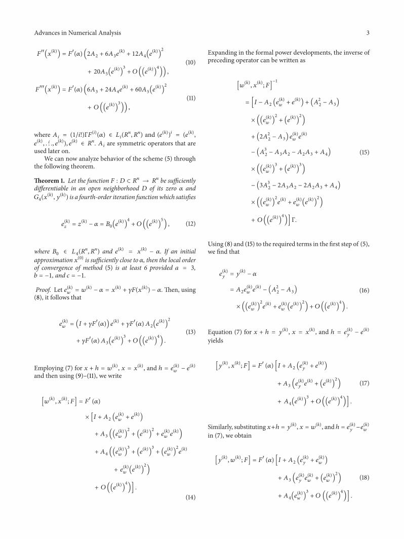
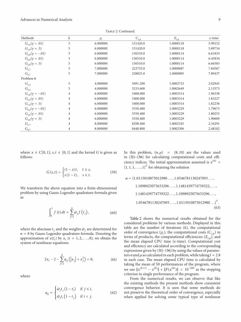