Representing flow mixing demands in a multi-nodal CDDP model of a mixed used catchment

I. Mahakalanda a, S. Dye a, E.G. Read a and S.R. Starkey a

a Department of Management, University of Canterbury, New Zealand. Email: indra.mahakalanda@pg.canterbury.ac.nz

Abstract: Constructive dual dynamic programming (CDDP) can be used to optimise a multi-nodal water system, or to clear a multi-nodal water market in the presence of competing consumptive demands, such as irrigation for farming, and non-consumptive demands, such as hydro-power generation. In this setting, CDDP is used in a two-stage process. First a deterministic multi-node version of the algorithm is used to construct a series of demand curves for release ( ) under various catchment inflow scenarios. This is termed the ‘intra-period’ problem. Then a stochastic version of the algorithm uses the constructed ’s to optimise the system, or clear the market over multiple periods, under uncertainty. This paper outlines the intra-period multi-node CDDP algorithm, and shows how to adapt this to address uses with water-mixing requirements, such as water returned to the river after being used for cooling a thermal power plant.

All cost and benefit functions at the nodes are converted to net demand functions, i.e., marginal net benefit as a function of water supplied. For this, the nodal marginal value (or bid) information is re-cast to form net demand curves, and the arcs re-oriented towards the reservoir. Then the algorithm constructs the intra-period demand curve for release ( ) by sequentially forming marginal water value curves at each node, passing these curves towards the reservoir. Arc flow bounds may limit the opportunities for using water at the nodes. Consumptive users extract water from the system, so each unit of water flow can only be used for a single consumptive use. A non-consumptive user transfers water from one node to another, extracting some benefit (e.g. from hydropower generation), or incurring some cost (e.g. for a pump). Costs can be associated with arc flow bounds and distributary demands to represent in-stream and environmental reserve flows enforced using penalty costs.

High temperature return flows from thermal power plant cooling can affect the downstream ecosystem. As a result an additional flow past the thermal station is needed to control the temperature. The mixing flow required can be modelled as a fixed ratio of heated to unheated water. The paper explains how to extend a CDDP model to incorporate flow mixing externalities into the model, using multiple parallel arcs. The model assumes a single long-term storage reservoir embedded in a catchment with a “tree-like” topology. Consumptive demands occur at the nodes. Non-consumptive demands appear on arcs. Cooling and temperature control flow demands are represented as parallel arcs assuming that an upstream flow unit can be diverted to any arc of our choice, but other types of flow splitting are discussed. The deterministic CDDP algorithm then forms a net conditional for each node that implicitly trades off the marginal value of all uses, to maximise total value, or clear the intra-period market. That can then be incorporated into a stochastic CDDP algorithm to construct (inter-period) marginal storage values for the reservoir (and implicit release/allocation schedules for the entire catchment) over the entire planning horizon.

Keywords: Water resource management, water markets, constructive dual dynamic programming, environmental management

20th International Congress on Modelling and Simulation, Adelaide, Australia, 1–6 December 2013 www.mssanz.org.au/modsim2013

2952

Mahakalanda et al., Representing flow mixing demands in a multi-nodal CDDP model of a mixed used catchment

1. INTRODUCTION

A large body of literature addresses the application of optimization models to the operation of hydro-reservoir systems. System size and inflow uncertainties can lead to high-dimensional stochastic models with non-linear objective functions. An optimization model with the primary objective of maximising hydropower production typically imposes hard constraints to meet non-generation requirements. Such constraints can reduce the economic value of hydropower production. In some cases, the non-generation water demands are not considered in planning. The increase in competing user demands, as witnessed in many places, may compromise the original operating targets when such approaches are used. Environmental constraints can also impose restrictions on flow. These range from simple flow bounds to more complicated requirements. In some places, thermal power plants may be located in close proximity to the river to make use of the water for cooling. For example, the Huntly thermal Power Station (HPS) in the Waikato region of New Zealand draws water for cooling purposes and subsequently discharges warmer water back into the Waikato River. Unless managed, the downstream temperature level may rise so much that it affects the river ecosystem. To address this, reservoir releases may be required to help regulate river flows under (1) hydropower production, (2) irrigation and urban water demands, (3) cooling flow demands, and (4) corresponding temperature control (mixing or diluting) flow demands. As a result, devising an operating policy to accommodate all the above requirements can be a challenging task.

This paper shows how to adapt a multi-nodal constructive dual dynamic programming (CDDP) approach to efficiently allocate water in a mixed used catchment in the presence of water mixing-type constraints. The rest of this paper is organized as follows. Section 2 describes relevant background literature. Section 3 presents a deterministic multi-nodal CDDP approach and how it could be extended to handle parallel paths, with mixing-type constraints. Section 4 then briefly describes how the multi-nodal deterministic CDDP can be embedded into a stochastic CDDP approach over a longer time-horizon to set up a market. Then, a numerical illustration is presented of the model applied to a hypothetical system styled on the Waikato river catchment.

2. BACKGROUND LITERATURE

Hydro-reservoir optimization models usually assume constant consumptive and in-stream flow demands and often hard constraints are imposed to satisfy them. Tilmant and Kelman (2007) considered additional constraints to represent consumptive diversions (nearly constant irrigation demands). Jacobs et al. (1995) modelled hydro scheduling problem by imposing hard constraints to meet consumptive demands. Generally, conflicting objectives can be explicitly incorporated into multi-objective optimization models (Ko et al., 1992). The water resource management literature extensively refers to models with non-hydro objectives (Rosegrant et al., 2000). However, the literature raises the issue of safeguarding environmental needs under competitive water trading demands. In reply, a number of studies have attempted to incorporate in-stream flow values to provide economic incentives to safeguard and upgrade ecological contributions. For example, Griffin and Hsu (1993) used an “environmental trustee”, or an in-stream flow district (IFD), to represent the collective environmental water demands. Later, Murphy et al. (2009) represented in-stream flow via an environmental agent.

The CDDP approach was initially used to solve the hydro-reservoir scheduling problem. It solves the dual of the standard DP reservoir optimization problem and implicitly optimises an operating policy similar to SDP for the entire planning horizon. But CDDP focusses on determining the primal storage state levels corresponding to a pre-defined grid of dual “state space” variables, typically marginal water value levels (and inflow states); see Read and Hindsberger (2010) for more details. One advantage of CDDP is that it uses an intra-period pre-computation approach that can employ any solution technique that produces a monotone demand curve (or surface) for release. The intra-period model might cover one or several sub-periods between the periods within the main (or inter-period) model. For example, Scott and Read (1996) incorporated an electricity market “gaming” model as the intra-period model. Later, Starkey et al. (2012) describe the application of the model developed by Dye et al. (2012) to clear an inter-period stochastic water market. Mahakalanda et al. (2012) developed an efficient deterministic CDDP algorithm to clear a multi-node market operating across a catchment, within a single period, while explicitly accounting for both consumptive and non-consumptive use, and environmental demands. This paper describes how this multi-nodal CDDP approach to intra-period optimisation, or market-clearing, can be embedded into a stochastic inter-period CDDP model, to optimise benefits, or clear markets, in a stochastic inter-period multi-nodal environment.

3. INTRA-PERIOD DETERMINISTIC MULTI-NODAL CDDP MODEL

An intra-period multi-nodal CDDP model is presented that constructs a demand curve for release from a long term reservoir, assuming known tributary flows, as described by Mahakalanda et al. (2012). The demand

2953

Mahakalanda et al., Representing flow mixing demands in a multi-nodal CDDP model of a mixed used catchment

curve for release provides the marginal value of the last unit released from long term storage, for any release level. The constructed demand curve can be used as part of a stochastic optimisation over a longer time horizon, or a market-clearing model, as described in the following section.

The CDDP approach constructs the demand curve for release directly from bid curves, or marginal cost and benefit functions. It effectively works directly with the optimality conditions of an underlying welfare maximisation model. The model is based on following assumptions:

The catchment network has a single long term storage reservoir and a tree structure. Consumptive and non-consumptive user benefits and costs are independent of those faced by other users,

and in other periods. Costs are convex (and benefits concave) piecewise linear functions of water use. The corresponding

marginal functions are thus piecewise constant, increasing and decreasing, respectively.

Each non-reservoir node ∈ 1,… , has a parent node, being the neighbouring node on the unique path towards the reservoir. A node’s parent may be either upstream or downstream, depending on how it is situated with respect to the reservoir. The CDDP algorithm produces a single (expected) intra-period at node 0, the reservoir, by aggregating the various water demand and supply curves for all other nodes, towards the reservoir.

Each node has between and units of tributary inflow available. Inflow at the reservoir could alternatively be accounted in the inter-temporal model. Variable represents the amount of this inflow captured at node i for use here or downstream, ≤ ≤ . Tributary inflows not captured (i.e., where < ) are assumed as a lost to the system. Let ( ) denote the convex cost function associated with the capture of this flow; this allows for supply participants who incur costs or who charge for the flow injection. For tributary inflows, the marginal cost is likely to be zero but could, for example, represent external opportunity costs. Each non-root node i has ≥ 0 units of (potential) consumptive demand, with an associated concave benefit function ( ). Variable 0 ≤ ≤ , represents the consumptive demand met at node i. All

units are assumed to be permanently withdrawn from the system. Variable 0 ≤ ≤ represents distributary flow from non-root node i. The target flow is (≥ 0), with a convex cost function ( − ) associated with missing the target. Distributary flows may be used to apply minimum environmental flow requirements.

Tributary flows form net demand function, ( ) = ( ) (1)

Consumptive demands form net demand function, ( ) = ( ) (2)

Distributary flows form net demand function, ( ) = ( ) (3)

Arc bounds , , on arcs between adjacent nodes ( , ) ∈ , represent minimum in-stream flow levels and flood/spill control requirements. Non-consumptive flow demands, , such as hydro generation, may also occur on arcs and imply marginal benefits which affect the demand curve for water at the parent node. Let denotes the arc flow volume. The multi-nodal CDDP algorithm uses optimality conditions to determine a net-demand curve for water at each node (Mahakalanda et al., 2012). Nodes are processed from the leaf nodes in towards the reservoir at the root. At each node, the various competing demands and supplies are transformed into net-demand functions. These are combined with the net-demand curves for water from any arcs leading away from the reservoir to create a nodal net-demand curve for water. Effectively, demands with larger marginal returns are served before those with lower marginal return. We abuse notation slightly by assuming all marginal cost/benefit functions have already been transformed to net-demand form. The net-demand curve for water can then be determined by sorting the marginal net-demands from highest to lowest, or equivalently by ‘horizontal addition’, which amounts to adding the function inverses: ( ) = + + + ∑( , )∈ ( ) (4)

The terms correspond to net-demands for water from child nodes, see below. Net-demand curves on arcs are processed from child to parent, by truncating the net-demand curve for water, , to the arc bounds, to form . Where an arc involves a non-consumptive demand, this adjusts the marginal benefit from each unit of flow directly.

2954

Mahakalanda et al., Representing flow mixing demands in a multi-nodal CDDP model of a mixed used catchment

This adjustment is accounted for by ‘vertically’ adding (or subtracting) the non-consumptive flow net-demand curve, , to (from) the child node’s net demand curve for water, , where the water flow is away from (towards) the reservoir. = + (5)

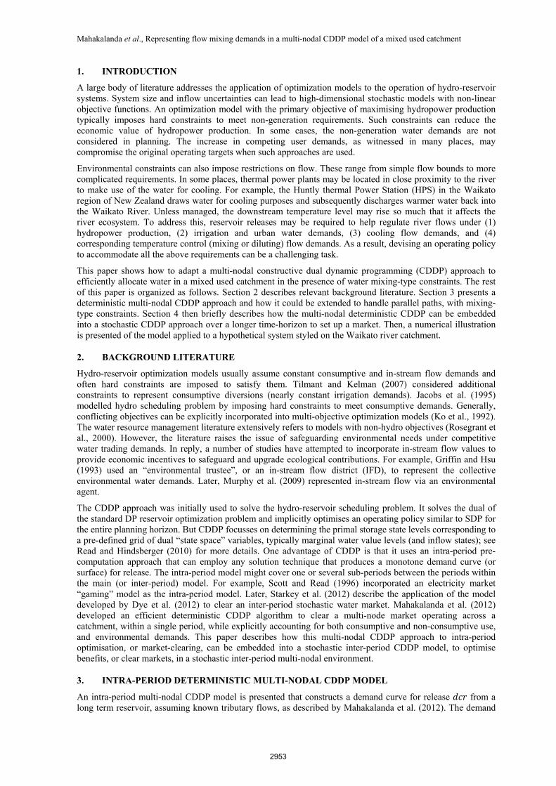
The demand curve for release constructed at the reservoir is guaranteed to be optimal as, by construction, the optimality conditions apply at each node in the catchment tree. Figure 1 below illustrates the multi-nodal CDDP processes for a simple catchment consisting of one reservoir, and one other node. On the LHS is a simple schematic of the reservoir (node 0) and the RHS illustrates how the various Marginal Water Value (mwv) curves are added horizontally (in the top graphs) and vertically (in the bottom graphs).

: 0,4

: 0,2

: −2,0

: −2,6 : 0,4

: 0,4 : 0,4

: 0,4

+ +

+

, = 0,4

Figure 1. An illustration of processing a node using the multi-nodal CDDP algorithm

The nodal demand curve for water at node 1, is constructed by horizontally adding consumptive demands, , distributary demands and tributary flow (net) demands . The net demand curve for water, , is

truncated using arc flow bounds = 0,4 before passing it to the parent node. The truncated nodal demand curve for water , and non-consumptive arc flow demand curve are then vertically added to form the nodal demand curve for flow at the parent node, .

The algorithm determines final water allocations, as a function of reservoir release, based on the marginal water values at the nodes and arcs. In this case, the distributary (environmental) flow demands were given absolute priority, and thus met using local tributary flows. But a trade-off could easily be modelled by applying several tiers of (increasing) penalties to violation of arc flow bounds. The next section shows how the multi-nodal chain optimization model (Mahakalanda et al., 2012) can flexibly handle parallel arcs between nodes.

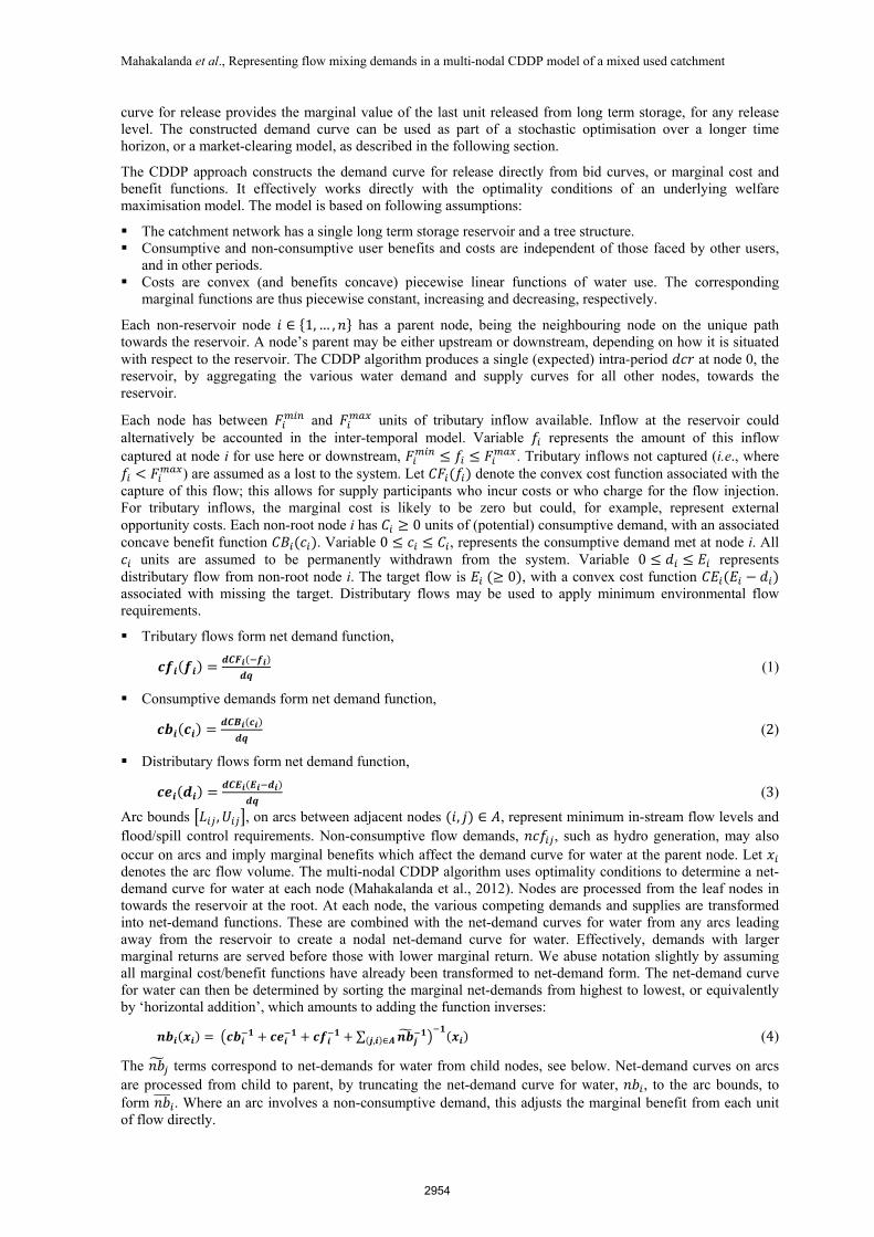
3.1 Processing parallel arcs

The above illustrated how non-consumptive benefits due to arc flows can be accounted for by vertically adding that marginal benefit curve to the for the parent node. This does not account for multiple parallel arcs between two nodes, or multiple simultaneous benefits arising from the same flow. In some cases, say, recreational, environmental and power generation, benefits may all arise simultaneously from the same flow. In others, a sluice gate might allow us to control the way flows are split between two parallel arcs, a boom might split flows in a constant ratio, or a weir might be designed to produce a split that varies with the flow level. The type of demand curve combination required (horizontal or vertical addition), is determined by the type of flow splitting applied.

Case 1: Controlled flow splitting

Under controlled flow spitting, the arc each unit of water is sent down can be chosen freely. For example, in the case of two parallel hydro-stations, a movable gate might be used to divert flows to one or the other. Let and denote the net-demand functions representing benefits from the two parallel paths. Since the path for each unit of water is freely chosen, CDDP can construct the composite arc flow demand curve by horizontally adding and as shown in the figure below. Effectively CDDP picks the next most valuable choice for each unit of water. In this case, CDDP can handle multiple competing non-consumptive uses on arcs in just the same way as it handles multiple competing consumptive uses at a node.

2955

Mahakalanda et al., Representing flow mixing demands in a multi-nodal CDDP model of a mixed used catchment

: 0,3 : 0,1

( ): 0,4

+

: 0,4 : 0,4

+

( )

Figure 3. Processing parallel arcs to provide cooling and temperature control flow demands

Case 2: Constant splitting of flows

At the opposite extreme, each flow unit may split in a constant ratio of, say, 0.25:0.75. The effect is the same as if the ratio defined the probability that a tiny increment flows one way, or the other. The resulting combined net-demand curve is found by vertically adding adjusted net-demand curves for the parallel arcs flows, as shown in Figure 2. Note that integer increments in the aggregate do not remain integer, once split. So steps in the aggregate curve are typically formed using parts of adjacent steps in the underlying curves. Note that, because only 5 units of flow are assumed to be feasible for ncf11 in the illustrated example, it ends up discarding those parts of each component that cannot be met.

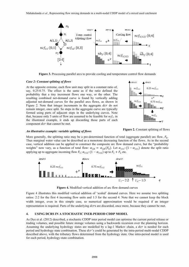
An illustrative example: variable splitting of flows

More generally, the splitting ratio may be a pre-determined function of total (aggregate parallel) arc flow, . Thus marginal water value can be described as a monotone decreasing function of the flows. As in the second case, vertical addition can be applied to construct the composite arc flow demand curve, but the “probability weights” now vary, as a function of total flow: = ( ). Let : (1 − ) denote the split ratio applying up to aggregate incoming flow ; : (1 − ) up to + etc.

+ 0.75

0.25

Figure 4. Modified vertical addition of arc flow demand curves

Figure 4 illustrates this modified vertical addition of ‘scaled’ demand curves. Here we assume two splitting ratios: 2:2 for the first 4 incoming flow units and 1:3 for the second 4. Note that we cannot keep the block width integer, even in this simple case, so numerical approximation would be required if an integer representation is required. Parts of the underlying s are discarded, once more, because they cannot be met.

4. USING DCRS IN A STOCHASTIC INER-PERIOD CDDP MODEL

As Dye et al. (2012) described, a stochastic CDDP inter period model can optimise the current period release or trading volumes, and possible future storage volumes using a backwards recursion over the planning horizon. Assuming the underlying hydrology states are modelled by a lag-1 Markov chain, a is needed for each period and hydrology state combination. These ’s could be generated by the intra-period multi-nodal CDDP described above, with the tributary flows determined from the hydrology state. One intra-period model is used for each period, hydrology-state combination.

0.75

0.25

+

Figure 2. Constant splitting of flows

2956

Mahakalanda et al., Representing flow mixing demands in a multi-nodal CDDP model of a mixed used catchment

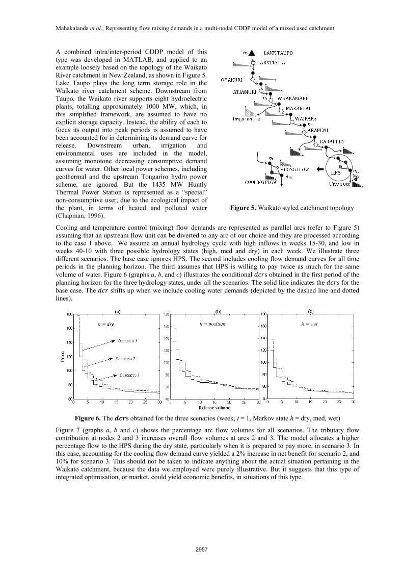
A combined intra/inter-period CDDP model of this type was developed in MATLAB, and applied to an example loosely based on the topology of the Waikato River catchment in New Zealand, as shown in Figure 5. Lake Taupo plays the long term storage role in the Waikato river catchment scheme. Downstream from Taupo, the Waikato river supports eight hydroelectric plants, totalling approximately 1000 MW, which, in this simplified framework, are assumed to have no explicit storage capacity. Instead, the ability of each to focus its output into peak periods is assumed to have been accounted for in determining its demand curve for release. Downstream urban, irrigation and environmental uses are included in the model, assuming monotone decreasing consumptive demand curves for water. Other local power schemes, including geothermal and the upstream Tongariro hydro power scheme, are ignored. But the 1435 MW Huntly Thermal Power Station is represented as a “special” non-consumptive user, due to the ecological impact of the plant, in terms of heated and polluted water (Chapman, 1996).

Cooling and temperature control (mixing) flow demands are represented as parallel arcs (refer to Figure 5) assuming that an upstream flow unit can be diverted to any arc of our choice and they are processed according to the case 1 above. We assume an annual hydrology cycle with high inflows in weeks 15-30, and low in weeks 40-10 with three possible hydrology states (high, med and dry) in each week. We illustrate three different scenarios. The base case ignores HPS. The second includes cooling flow demand curves for all time periods in the planning horizon. The third assumes that HPS is willing to pay twice as much for the same volume of water. Figure 6 (graphs a, b, and c) illustrates the conditional s obtained in the first period of the planning horizon for the three hydrology states, under all the scenarios. The solid line indicates the s for the base case. The shifts up when we include cooling water demands (depicted by the dashed line and dotted lines).

Figure 6. The s obtained for the three scenarios (week, t = 1, Markov state h = dry, med, wet)

Figure 7 (graphs a, b and c) shows the percentage arc flow volumes for all scenarios. The tributary flow contribution at nodes 2 and 3 increases overall flow volumes at arcs 2 and 3. The model allocates a higher percentage flow to the HPS during the dry state, particularly when it is prepared to pay more, in scenario 3. In this case, accounting for the cooling flow demand curve yielded a 2% increase in net benefit for scenario 2, and 10% for scenario 3. This should not be taken to indicate anything about the actual situation pertaining in the Waikato catchment, because the data we employed were purely illustrative. But it suggests that this type of integrated optimisation, or market, could yield economic benefits, in situations of this type.

Figure 5. Waikato styled catchment topology

2957

Mahakalanda et al., Representing flow mixing demands in a multi-nodal CDDP model of a mixed used catchment

Figure 7. Arc flows (volume) as a percentage of release recorded for the three scenarios (week, t =1)

5. CONCLUSIONS

This paper has described a nodal catchment model that can implicitly maximise value and/or clears an inter-temporal multi-nodal market in the presence of uncertain flows. It assumes a single reservoir catchment with a tree configuration. Cooling and temperature control flow demands are represented on parallel arcs that can be processed as for normal arc flow demands. We model these flow requirements assuming that an upstream flow unit can be diverted to any arc of our choice, but other assumptions can be made. The multi-nodal deterministic CDDP then constructs an aggregate for each node in each period. Aggregate demand curves for storage in the long term reservoir were then constructed using the stochastic CDDP algorithm. While applied here to an example involving hydro power production and mixing of thermal power station cooling water, the technique could be applied in a variety of situations in which flow mixing is important for other reasons, such as dilution of polluted water flows. The results demonstrate how net benefits can be increased by accounting for the demand curve for cooling water, across all hydrology conditions and time periods.

REFERENCES

Chapman, M. A. (1996). Human impacts on the Waikato river system, New Zealand. GeoJournal, 40(1-2), 85-99.

Dye, S., Read, E. G., Read, R. A., & Starkey, S. R. (2012). Easy Implementations of Generalised Stochastic CDDP Models for Market Simulation Studies, Paper presented at the 4th IEEE and Cigré International Workshop on Hydro Scheduling in Competitive Markets, Bergen, Norway, June 14-15.

Griffin, R. C., & Hsu, S. H. (1993). The potential for water market efficiency when instream flows have value. American Journal of Agricultural Economics,75(2), 292-303.

Jacobs, J., Freeman, G., Grygier, J., Morton, D., Schultz, G., Staschus, K., & Stedinger, J. (1995). SOCRATES: A system for scheduling hydroelectric generation under uncertainty. Annals of Operations Research, 59(1), 99-133.

Ko, S. K., Fontane, D. G., & Labadie, J. W. (1992). Multi-objective optimization of reservoir systems operation. JAWRA Journal of the American Water Resources Association, 28(1), 111-127.

Mahakalanda, I., Dye, S., Read, E.G. and Raffensperger, J.,F., (2012). Intra-period Market Clearing for a Multi-Use Catchment via CDDP, Paper presented at the ORSNZ Conference, Wellington, New Zealand, December 10-11.

Murphy, J. J., Dinar, A., Howitt, R. E., Rassenti, S. J., Smith, V. L., & Weinberg, M. (2009). The design of water markets when instream flows have value. Journal of environmental management, 90(2), 1089-1096.

Read, E. G., & Hindsberger, M. (2010). Constructive dual DP for reservoir optimization. Handbook of Power Systems I, 3-32.

Scott, T. J., & Read, E. G. (1996). Modelling hydro reservoir operation in a deregulated electricity market. International Transactions in Operational Research, 3(3), 243-253.

Starkey, S. R., Dye, S., Read, E. G. & Read, R. A. (2012). Stochastic versus deterministic market design: some experimental results, Paper presented at the 4th IEEE and Cigré International Workshop on Hydro Scheduling in Competitive Markets, Bergen, Norway, June 14-15.

Rosegrant, M. W., Ringler, C., McKinney, D. C., Cai, X., Keller, A., & Donoso, G. (2000). Integrated economic‐hydrologic water modeling at the basin scale: The Maipo River basin. Agricultural economics, 24(1), 33-46.

Tilmant, A., & Kelman, R. (2007). A stochastic approach to analyze trade-offs and risks associated with large-scale water resources systems. Water resources research, 43(6), W06425.

2958