Report No. CCEER 13-15 - American Iron and Steel Institute/media/Files/SMDI/Construction/Bridges -...
158
Report No. CCEER 13-15 SEISMIC DESIGN AND NONLINEAR EVALUATION OF STEEL I-GIRDER BRIDGES USING CONVENTIONAL AND DUCTILE SUPPORT CROSS-FRAMES Ahmad M. Itani Eric V. Monzon Michael A. Grubb Ebrahim Amirihormozaki Center for Civil Engineering Earthquake Research University of Nevada, Reno September 2013
Transcript of Report No. CCEER 13-15 - American Iron and Steel Institute/media/Files/SMDI/Construction/Bridges -...

Report No. CCEER 13-15
SEISMIC DESIGN AND NONLINEAR
EVALUATION OF STEEL I-GIRDER BRIDGES
USING CONVENTIONAL AND DUCTILE
SUPPORT CROSS-FRAMES
Ahmad M. Itani
Eric V. Monzon
Michael A. Grubb
Ebrahim Amirihormozaki
Center for Civil Engineering Earthquake Research
University of Nevada, Reno
September 2013

i
Abstract
The AASHTO Guide Specifications for LRFD Seismic Bridge Design define three Global Seismic
Design Strategies based on the expected behavior characteristics of bridge systems. The Type 2 design
strategy is dedicated to an essentially elastic substructure with a ductile superstructure. This category
applies to steel superstructures where the nonlinear response is achieved by providing ductile elements in
the interior pier support cross-frames. However, the current guide specifications do not provide bridge
engineers with a complete design procedure for achieving the desired performance when utilizing this
strategy. In an attempt to overcome this shortcoming, this report presents a proposed Force-Based design
procedure that will achieve an essentially elastic substructure and ductile superstructure. The proposed
language and modifications are based on the ASSHTO LRFD Specifications. The flexural resistance of
the reinforced concrete (R/C) substructure is based on the longitudinal seismic forces that are determined
from the design spectrum using a force reduction factor equal to 1.5. Meanwhile, the shear resistance of
the substructure is conservatively based on assumed plastic hinging of the substructure, which is not
expected to occur. The pier support cross frames are designed and detailed to achieve a ductile response.
The horizontal resistance of these cross frames is based on the nominal shear resistance of the
substructure in the transverse direction divided by a response modification factor equal to 4. This will
ensure that the superstructure will act as a ‗fuse‘ and will not subject the substructure to forces that may
cause a nonlinear response in the transverse direction. The shear resistance of the substructure is also
checked based on the expected lateral resistance of fully yielded and strain hardened pier support cross
frames. In order to achieve a ductile response of the pier support cross frames, the diagonal members,
which are expected to undergo inelastic response, are detailed to satisfy more stringent width-to-thickness
and slenderness ratio limits. The diagonal member connections and other cross frame members are
designed for fully yielded and strain hardened diagonal members.
Three example bridges were selected to illustrate the proposed design procedure for the Type 2 design
strategy. The substructure of these bridges was varied to examine single-column piers, two-column piers,
and wall piers. Examples showing the design of these bridges using the more conventional Type 1 design
strategy are also shown. Thus, a total of six bridge design examples are shown in this report. The seismic
performance of these design examples was then evaluated through nonlinear response history analysis
using ground motions representing the design and maximum considered earthquakes.
The results of the nonlinear analysis for the Design and the MCE Levels earthquakes showed that the
proposed strategy indeed achieved an essentially elastic substructure and the inelasticity was concentrated
at the pier cross-frames as intended. Using the proposed design strategy resulted in an increase in the size
of the substructure; however the seismic performance was greatly enhanced with minimal post-earthquake
damage. The damage was limited to the diagonals of the pier support cross frames. These members can be
easily replaced after large earthquake without interruption of the traffic. Meanwhile in conventional
design, the size of the pier cross frames and the bearings were significantly larger than those in bridge
designed according to the proposed strategy. Furthermore, as intended, the damage was concentrated in
the substructure which will require substantial repair after major earthquakes. It is important to note here
that for bridges with pier walls designed according to the conventional seismic design, the pier cross
frames buckled under the design level earthquake. This damage is not intended to occur and may have
detrimental effect on the performance of connections and the bearings.

ii
Acknowledgement
The work on this report was funded by American Iron and Steel Institute, AISI, contract CC-3070. Mr.
Dan Snyder was the contract manager. The authors sincerely appreciate his support and collaboration.
The authors appreciate the comments by a task group funded by AASHTO to support HSCOBS Technical
Committee on Seismic Design. The chair of this group is Dr. Lee Marsh. The authors wish to thank the
following individuals for their help and suggestions: Mr. Richard Pratt, Mr. Greg Perfetti, Prof. Ian
Buckle, Dr. John Kulicki, Dr. Elmer Marx, Dr. Lian Duan, Mr. Keith Fulton, and Dr. Gichuru Muchane.
Disclaimer
The materials set fourth here in are for general information only. They are not a substitute for competent
professional assistance. The opinions expressed in this report are those of the authors and do not
necessarily represents the views of the University of Nevada, Reno, the American Iron and Steel Institute
and the individuals who kindly provided the authors information and comments.

iii
Table of Contents
Abstract .......................................................................................................................................................... i
Acknowledgement ........................................................................................................................................ ii
Disclaimer ..................................................................................................................................................... ii
Table of Contents ......................................................................................................................................... iii
Chapter 1 Introduction ............................................................................................................................... 1
1.1 Background ................................................................................................................................... 1
1.2 Proposed Draft AASHTO Specifications for the Type 2 Design Strategy ................................... 1
1.3 Seismic Design Examples ........................................................................................................... 16
1.3.1 Set I Bridges ........................................................................................................................ 16
1.3.2 Set II Bridges ...................................................................................................................... 17
1.3.3 Set III Bridges ..................................................................................................................... 18
1.4 Seismic Design Methodology ..................................................................................................... 18
1.5 Presentation of Design Examples ............................................................................................... 20
1.6 Analytical Model ........................................................................................................................ 20
1.6.1 Material Properties .............................................................................................................. 20
1.6.2 Superstructure ..................................................................................................................... 21
1.6.3 Support Cross-Frames ......................................................................................................... 23
1.6.4 Pier Caps and Columns ....................................................................................................... 23
1.6.5 Abutment Backfill Soil ....................................................................................................... 24
1.7 Design Loads .............................................................................................................................. 24
1.8 Seismic Evaluation of Design Examples .................................................................................... 28
1.8.1 Ground Motions .................................................................................................................. 28
Chapter 2 Example I-1: Bridge with Single-Column Piers Designed using the Type 1 Strategy ........... 32
2.1 Bridge Description ...................................................................................................................... 32
2.2 Computational Model ................................................................................................................. 32
2.3 Analysis....................................................................................................................................... 33
2.3.1 Gravity Loads – DC and DW .............................................................................................. 33
2.3.2 Earthquake Loads – EQ ...................................................................................................... 35
2.3.3 Design Loads ...................................................................................................................... 38
2.4 Design of Columns ..................................................................................................................... 39
2.5 Seismic Design of Support Cross-Frames................................................................................... 41

iv
2.6 Cross-Frame Properties for Nonlinear Analysis ......................................................................... 44
2.7 Design Summary ......................................................................................................................... 46
2.8 Nonlinear Evaluation of Seismic Design .................................................................................... 47
2.8.1 Response under Design Earthquake .................................................................................... 47
2.8.2 Response under Maximum Considered Earthquake ........................................................... 47
Chapter 3 Example I-2: Bridge with Single-Column Piers Designed using the Type 2 Strategy ........... 50
3.1 Bridge Description ...................................................................................................................... 50
3.2 Computational Model ................................................................................................................. 50
3.3 Analysis....................................................................................................................................... 51
3.3.1 Gravity Loads – DC and DW .............................................................................................. 51
3.3.2 Earthquake Loads – EQ ...................................................................................................... 53
3.3.3 Design Loads ...................................................................................................................... 55
3.4 Design of Columns ..................................................................................................................... 56
3.5 Design of Support Ductile End Cross-Frames ............................................................................ 59
3.6 Cross-Frame Properties for Nonlinear Analysis ......................................................................... 62
3.7 Design Summary ......................................................................................................................... 63
3.8 Nonlinear Evaluation of Seismic Design .................................................................................... 64
3.8.1 Response under Design Earthquake .................................................................................... 64
3.8.2 Response under Maximum Considered Earthquake ........................................................... 64
Chapter 4 Example II-1: Bridge with Two-Column Piers Designed using the Type 1 Strategy ............. 69
4.1 Bridge Description ...................................................................................................................... 69
4.2 Computational Model ................................................................................................................. 69
4.3 Analysis....................................................................................................................................... 70
4.3.1 Gravity Loads – DC and DW .............................................................................................. 70
4.3.2 Earthquake Loads – EQ ...................................................................................................... 72
4.3.3 Design Loads ...................................................................................................................... 75
4.4 Design of Columns ..................................................................................................................... 76
4.5 Seismic Design Support of Cross-Frames................................................................................... 81
4.6 Cross-Frame Properties for Nonlinear Analysis ......................................................................... 83
4.7 Design Summary ......................................................................................................................... 84
4.8 Performance Assessment ............................................................................................................ 85
4.8.1 Response under Design Earthquake .................................................................................... 85
4.8.2 Response under Maximum Considered Earthquake ........................................................... 85

v
Chapter 5 Example II-2: Bridge with Two-Column Piers Designed using the Type 2 Strategy ............. 89
5.1 Bridge Description ...................................................................................................................... 89
5.2 Computational Model ................................................................................................................. 89
5.3 Analysis....................................................................................................................................... 90
5.3.1 Gravity Loads – DC and DW .............................................................................................. 90
5.3.2 Earthquake Loads – EQ ...................................................................................................... 92
5.3.3 Design Loads ...................................................................................................................... 94
5.4 Design of Columns ..................................................................................................................... 95
5.5 Design of Support Ductile Cross-Frames ................................................................................... 99
5.6 Cross-Frame Properties for Nonlinear Analysis ....................................................................... 102
5.7 Design Summary ....................................................................................................................... 103
5.8 Performance Assessment .......................................................................................................... 104
5.8.1 Response under Design Earthquake .................................................................................. 104
5.8.2 Response under Maximum Considered Earthquake ......................................................... 104
Chapter 6 Example III-1: Bridge with Wall Piers Designed using the Type 1 Strategy ....................... 108
6.1 Bridge Description .................................................................................................................... 108
6.2 Computational Model ............................................................................................................... 108
6.3 Analysis..................................................................................................................................... 111
6.3.1 Gravity Loads – DC and DW ............................................................................................ 111
6.3.2 Earthquake Loads – EQ .................................................................................................... 111
6.3.3 Design Loads .................................................................................................................... 114
6.4 Design of Wall Pier ................................................................................................................... 115
6.5 Seismic Design of Support Cross-Frames................................................................................. 118
6.6 Cross-Frame Properties for Nonlinear Analysis ....................................................................... 120
6.7 Design Summary ....................................................................................................................... 121
6.8 Performance Assessment .......................................................................................................... 122
6.8.1 Response under Design Earthquake .................................................................................. 122
6.8.2 Response under Maximum Considered Earthquake ......................................................... 122
Chapter 7 Example III-2: Bridge with Wall Piers Designed using the Type 2 Strategy ....................... 127
7.1 Bridge Description .................................................................................................................... 127
7.2 Computational Model ............................................................................................................... 127
7.3 Analysis..................................................................................................................................... 130
7.3.1 Gravity Loads – DC and DW ............................................................................................ 130
vi
7.3.2 Earthquake Loads – EQ .................................................................................................... 130
7.3.3 Design Loads .................................................................................................................... 132
7.4 Design of Wall Pier ................................................................................................................... 133
7.5 Design of Support Ductile Cross-Frames ................................................................................. 135
7.6 Cross-Frame Properties for Nonlinear Analysis ....................................................................... 138
7.7 Design Summary ....................................................................................................................... 139
7.8 Performance Assessment .......................................................................................................... 140
7.8.1 Response under Design Earthquake .................................................................................. 140
7.8.2 Response under Maximum Considered Earthquake ......................................................... 140
Chapter 8 Summary of Designs and Nonlinear Evaluation ................................................................... 143
8.1 Overview ................................................................................................................................... 143
8.2 Design Summary ....................................................................................................................... 143
8.3 Summary of Nonlinear Design Evaluation ............................................................................... 145
References ................................................................................................................................................. 150

1
Chapter 1 Introduction
1.1 Background
A ductile superstructure with an essentially elastic substructure commonly known as Type 2 Design
Strategy may be used as an alternative to the conventional seismic design strategy of providing an elastic
superstructure and a ductile substructure. The ductile superstructure elements must be specially designed
and detailed to undergo large cyclic deformations without premature failure. The inelastic activity in these
elements will dissipate seismic energy and will limit the seismic forces transferred to the substructure. In
this design strategy, special cross-frames are provided at the interior-pier supports. The substructure in
this case is designed to be essentially elastic in the longitudinal and transverse directions of the bridge.
Ideally, ductile superstructures have shown the most effectiveness when used with stiff substructures.
Flexible substructures will attract smaller seismic forces and, thus, the support cross-frames will be
subjected to low seismic forces and will be less effective (Alfawakhiri and Bruneau, 2001; Bahrami et al.,
2010).
The special ductile support cross-frames are designed with an R factor equal to 4.0. Thus, the diagonal
members of these cross frames will undergo a nonlinear response and will limit the seismic forces in the
transverse direction. Experimental investigations were conducted on diagonal cross-frame members and
subassemblies to determine the nonlinear response of single angles to ensure that they will be able to
withstand large cyclic deformations without premature failure. These experiments also provided the
physical data needed to establish the overstrength factor for the diagonal members and their failure mode
(Carden et al., 2006). Nonlinear response history analyses conducted on 3D bridge models confirmed the
seismic response predicted by the proposed seismic design procedure.
1.2 Proposed Draft AASHTO Specifications for the Type 2 Design Strategy
The following are proposed force-based draft specifications for possible consideration and evaluation that
would incorporate the Type 2 Design Strategy in Article 6.16 of the AASHTO LRFD Bridge Design
Specifications. Revisions to the AASHTO Guide Specifications for LRFD Seismic Bridge Design, which
are displacement based specifications, are not proposed herein:
6.16.4.5Ductile Superstructures
6.16.4.5.1General
For a ductile superstructure, special support cross-
frames, designed as specified in Article 6.16.4.5.2, shall be
provided at all interior supports. The substructure shall be
designed to be essentially elastic as specified in Article
4.6.2.8.2.
C6.16.4.5.1
A ductile superstructure with an essentially elastic
substructure may be used as an alternative to an elastic
superstructure in combination with a ductile
substructure. Ductile superstructures must be specially
designed and detailed to dissipate seismic energy. In

2
The seismic design forces for the diagonal members of
the special support cross-frames shall be taken as the
unreduced elastic seismic forces divided by a response
modification factor, R, which shall be taken equal to 4.0.
The superstructure drift, determined as the ratio of
the relative lateral displacement of the girder top and
bottom flanges to the total depth of the steel girder, shall
not exceed 4%. The drift shall be determined from the
results of an elastic analysis.
ductile superstructures, special support cross-frames are
to be provided at all interior supports and must be
detailed and designed to undergo significant inelastic
activity and dissipate the seismic input energy without
premature failure or strength degradation in order to
limit the seismic forces on the substructure. The
substructure in this case is designed to be essentially
elastic as specified in Article 4.6.2.8.2 and described in
Article C6.16.4.1. This strategy has been analytically
and experimentally validated using subassembly and
shake table experiments on steel I-girder bridges with no
skew or horizontal curvature.
Ideally ductile superstructures have shown the most
effectiveness when utilized in conjunction with stiff
substructures. Flexible substructures will attract smaller
seismic forces, and thus, the special support cross-frames
will also be subjected to smaller seismic forces and will
be less effective (Alfawakhiri and Bruneau, 2001).
Bridge dynamic analyses conducted according to the
provisions of Article 4.7.4 can provide insight on the
effectiveness of special support cross-frames
(Alfawakhiri and Bruneau, 2001; Bahrami et al., 2010;
and Itani et al., 2013).
The R factor of 4.0 specified for the design of the
special support cross-frame diagonal members in a
ductile superstructure is the result of nonlinear time
history analyses conducted on 3D bridge models
(Bahrami et al., 2010 and Itani et al., 2013). For these
nonlinear analyses, the deck and steel plate girders were
modeled with shell elements, while the cross-frames, cap
beams and columns were modeled with nonlinear frame
elements.
The drift, , of the superstructure is to be
determined from an elastic structural analysis without
the use of an R value.
6.16.4.5.2Special Support Cross-Frames
Special support cross-frames shall consist of top and
bottom chords and diagonal members. The diagonal
members shall be configured either in an X-type or an
inverted V-type configuration. Only single angles or
double angles with welded end connections shall be
permitted for use as members of special support cross-
frames.
In an X-type configuration, diagonal members shall be
connected where the members cross by welds. The welded
connection at that point shall have a nominal resistance
equal to at least 0.25 times the tensile resistance of the
diagonal member, Pt, determined as specified in Article
6.16.4.5.2c.
In both configurations, the top chord shall be designed
for an axial force taken as the horizontal component of the
tensile resistance of the diagonal member, Pt, determined
C6.16.4.5.2
Concentric support cross-frames are those in which
the centerlines of members intersect at a point to form a
truss system that resists lateral loads. Concentric
configurations that are permitted for special support
cross-frames in ductile superstructures are X-type and
inverted V-type configurations. The use of tension-only
bracing in any configuration is not permitted. V-type
configurations and solid diaphragms are also not
permitted. Members other than single-angle or double-
angle members are not currently permitted, as other
types of members have not yet been sufficiently studied
for potential use in special support cross-frames (AISC,
2010b and Bahrami et al., 2010).
The required resistance of the welded connection at
the point where diagonal members cross in X-type
configurations is intended to permit the unbraced length

3
as specified in Article 6.16.4.5.2c.
In an inverted V-type configuration, the top chord and
the concrete deck at the location where the diagonals
intersect shall be designed to resist a vertical force, Vt,
taken equal to:
sin3.0 nctt PPV (6.16.4.5.2-1)
where:
= angle of inclination of the diagonal member with
respect to the horizontal (degrees)
Pnc = nominal compressive resistance of the diagonal
member determined as specified in Article
6.16.4.5.2c (kip)
Pt = tensile resistance of the diagonal member
determined as specified in Article 6.16.4.5.2c
(kip)
Members of special support cross-frames in either
configuration shall satisfy the applicable requirements
specified in Articles 6.16.4.5.2a through 6.16.4.5.2e. The
welded end connections of the special support cross-frame
members shall satisfy the requirements specified in Article
6.16.4.5.3.
for determining the compressive buckling resistance of
the member to be taken as half of the full length (Goel
and El-Tayem, 1986; Itani and Goel, 1991; Carden et al.,
2005a and 2005b, and Bahrami et al., 2010).
Inverted V-type configurations exhibit a special
problem that sets them apart from X-type configurations.
Under lateral displacement after the compression
diagonal buckles, the top chord of the cross-frame and
the concrete deck will be subjected to a vertical
unbalanced force. This force will continue to increase
until the tension diagonal starts to yield. This unbalanced
force is equal to the vertical component of the difference
between the tensile resistance of the diagonal member
and the absolute value of 0.3Pnc. 0.3Pnc is taken as the
nominal post-buckling compressive resistance of the
member (Carden et al., 2006a). A similar overstrength
factor is applied in the design of the welded end
connections for special support cross-frame members in
Article 6.16.4.5.3, and in determining the transverse
seismic force on the piers/bents for the design of the
essentially elastic substructure in Article 4.6.2.8.2.
During a moderate to severe earthquake, special
support cross-frames and their end connections are
expected to undergo significant inelastic cyclic
deformations into the post-buckling range. As a result,
reversed cyclic rotations occur at plastic hinges in much
the same way as they do in beams. During severe
earthquakes, special support cross-frames are expected
to undergo 10 to 20 times the yield deformation. In
order to survive such large cyclic deformations without
premature failure, the elements of special support cross-
frames and their connections must be properly designed
(Zahrai and Bruneau, 1999a and 1999b; Zahrai and
Bruneau, 1998; Carden et al., 2006, and Bahrami et al.,
2010).
The requirements for the seismic design of special
support cross-frames are based on the seismic
requirements for Special Concentric Braced Frames
(SCBFs) given in AISC (2010b). These requirements are
mainly based on sections and member lengths that are
more suitable for building construction. However,
Carden et al. (2006) and Bahrami et al. (2010) tested
more typical sections and member lengths utilized in
bridge construction and verified that the AISC seismic
provisions for SCBFs can be used for the seismic design
of special support cross-frames. These studies, in
addition to other analytical and experimental
investigations conducted by numerous researchers, have
identified three key parameters that affect the ductility of
cross-frame members:
Width-to-thickness ratio;
Slenderness ratio; and
End conditions.

4
During earthquake motions, the cross-frame member
will be subjected to cyclic inelastic deformations. The
plot of the axial force versus the axial deformation of the
inelastic member is often termed a hysteresis loop. The
characterization of these loops is highly dependent on
the aforementioned parameters. Satisfaction of the
requirements related to these parameters specified in
Articles 6.16.4.5.2a through 6.16.4.5.2e will help to
ensure that the diagonal members of special support
cross-frames can undergo large inelastic cyclic
deformations without premature fracture and strength
degradation when subjected to the design seismic forces.
6.16.4.5.2aWidth-to-Thickness Ratio
Diagonal members of special support cross-frames
shall satisfy the following ratio:
yF
E3.0
t
b
(6.16.4.5.2a-1)
where:
b = full width of the outstanding leg of the angle (in.)
t = thickness of the outstanding leg of the angle (in.)
C6.16.4.5.2a
Traditionally, diagonal cross-frame members have
shown little or no ductility during a seismic event after
overall member buckling, which produces plastic hinges
at the mid-point of the member and at its two ends. At a
plastic hinge, local buckling can cause large strains,
leading to fracture at small deformations. It has been
found that diagonal cross-frame members with ultra-
compact elements are capable of achieving significantly
more ductility by forestalling local buckling (Astaneh-
Asl et al., 1985, Goel and El-Tayem, 1986). Therefore,
width-to-thickness ratios of outstanding legs of special
support cross-frame diagonal members are set herein to
not exceed the requirements for ultra-compact elements
taken from AISC (2010b) in order to minimize the
detrimental effect of local buckling and subsequent
fracture during repeated inelastic cycles.

5
6.16.4.5.2b Slenderness Ratio
Diagonal members of special support cross-frames
shall satisfy the following ratio:
yF
E0.4
r
K
(6.16.4.5.2b-1)
where:
K = effective length factor in the plane of buckling
determined as specified in Article 4.6.2.5
= unbraced length (in.). For members in an X-type
configuration, shall be taken as one-half the
length of the diagonal member.
r = radius of gyration about the axis normal to the
plane of buckling (in.)
C6.16.4.5.2b
The hysteresis loops for special support cross-
frames with diagonal members having different
slenderness ratios vary significantly. The area enclosed
by these loops is a measure of that component‘s energy
dissipation capacity. Loop areas are greater for a stocky
member than for a slender member; hence, the
slenderness ratio of diagonal members in special support
cross-frames is limited accordingly herein to the
requirement for stocky members in SCBFs given in
AISC (2010b).
6.16.4.5.2c Tensile and Nominal Compressive
Resistance
The tensile resistance, Pt, of diagonal members of
special support cross-frames shall be taken as:
nyyt PRP 2.1 (6.16.4.5.2c-1)
where:
Pny = nominal tensile resistance for yielding in the gross
section of the diagonal member determined as
specified in Article 6.8.2 (kip)
Ry = ratio of the expected yield strength to the
specified minimum yield strength of the diagonal
member determined as specified in Article 6.16.2
The nominal compressive resistance, Pnc, of diagonal
members of special support cross-frames shall be taken as:
nnc PP (6.16.4.5.2c-3)
where:
Pn = nominal compressive resistance of the diagonal
member determined as specified in Article 6.9.4.1
using an expected yield strength, RyFy (kip)
C6.16.4.5.2c
The diagonal members of special support cross-
frames are designed and detailed to act as ―fuses‖ during
seismic events to dissipate the input energy. These
members will experience large cyclic deformations
beyond their expected yield and compressive resistances.
The limitations on the width-to-thickness and
slenderness ratios specified in the preceding articles will
allow the diagonals of the special support cross-frames
to go through significant yielding and strain hardening
prior to fracture. The tensile resistance of diagonal
members of special support cross-frames, Pt, is to be
determined using an expected yield strength, RyFy
(AISC, 2010b). The resulting resistance is then
multiplied by a factor of 1.2 in Eq. 6.16.4.5.2c-1. This
factor is the upper bound of the ratio of Pt to the
expected nominal tensile resistance, RyPny, of the
diagonal members as determined experimentally by
Carden et al. (2006).
The nominal compressive resistance of diagonal
members of special support cross-frames, Pnc, is also to
be determined using an expected yield strength, RyFy,
according to Eq. 6.16.4.5.2c-3.

6
6.16.4.5.2dLateral Resistance
The lateral resistance, Vlat, of a special support cross-
frame in a single bay between two girders shall be taken as
the sum of the horizontal components of the tensile
resistance and the nominal post-buckling compressive
resistance of the diagonal members, or:
cos3.0 nctlat PPV (6.16.4.5.2d-1)
where:
= angle of inclination of the diagonal member with
respect to the horizontal (degrees)
Pnc = nominal compressive resistance of the diagonal
member determined as specified in Article
6.16.4.5.2c (kip)
Pt = tensile resistance of the diagonal member
determined as specified in Article 6.16.4.5.2c
(kip)
C6.16.4.5.2d
During seismic events, special support cross-frames
are expected to undergo large cyclic deformations. The
tension diagonal will yield and strain harden while the
compression diagonal will buckle. The dissipated energy
from this system depends on the ability of the tension
diagonal to undergo large deformations without
premature fracture. Furthermore, the compression
diagonal should also be able to withstand large
deformations without fracture due to local and global
buckling. Hence, the lateral resistance of a special
support cross-frame in a single bay is to be taken equal
to the sum of the horizontal components of the tensile
resistance and the nominal post-buckling compressive
resistance of the diagonal members. Carden et al.
(2006a) showed experimentally that for angle sections
satisfying the limiting width-to-thickness and
slenderness ratios specified in Articles 6.16.4.5.2a and
6.16.4.5.2b, respectively, the nominal post-buckling
compressive resistance of a diagonal member may be
taken equal to 0.3 times Pnc.
6.16.4.5.2eDouble-Angle Compression
Members
Double angles used as diagonal compression members
in special support cross-frames shall be interconnected by
welded stitches. The spacing of the stitches shall be such
that the slenderness ratio, /r, of the individual angle
elements between the stitches does not exceed 0.4 times
the governing slenderness ratio of the member. Where
buckling of the member about its critical buckling axis
does not cause shear in the stitches, the spacing of the
stitches shall be such that the slenderness ratio, /r, of the
individual angle elements between the stitches does not
exceed 0.75 times the governing slenderness ratio of the
member. The sum of the nominal shear resistances of the
stitches shall not be less than the nominal tensile resistance
of each individual angle element.
The spacing of the stitches shall be uniform. No less
than two stitches shall be used per member.
C6.16.4.5.2e
More stringent spacing and resistance requirements
are specified for stitches in double-angle diagonal
members used in special support cross-frames than for
conventional built-up members subject to compression
(Aslani and Goel, 1991). These requirements are
indented to restrict individual element buckling between
the stitch points and consequent premature fracture of
these members during a seismic event.
7
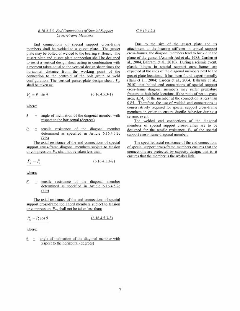
6.16.4.5.3End Connections of Special Support
Cross-Frame Members
End connections of special support cross-frame
members shall be welded to a gusset plate. The gusset
plate may be bolted or welded to the bearing stiffener. The
gusset plate and gusset plate connection shall be designed
to resist a vertical design shear acting in combination with
a moment taken equal to the vertical design shear times the
horizontal distance from the working point of the
connection to the centroid of the bolt group or weld
configuration. The vertical gusset-plate design shear, Vg,
shall be taken as:
sintg PV (6.16.4.5.3-1)
where:
= angle of inclination of the diagonal member with
respect to the horizontal (degrees)
Pt = tensile resistance of the diagonal member
determined as specified in Article 6.16.4.5.2c
(kip)
C.6.16.4.5.3
Due to the size of the gusset plate and its
attachment to the bearing stiffener in typical support
cross-frames, the diagonal members tend to buckle in the
plane of the gusset (Astaneh-Asl et al., 1985; Carden et
al., 2004, Bahrami et al., 2010). During a seismic event,
plastic hinges in special support cross-frames are
expected at the ends of the diagonal members next to the
gusset plate locations. It has been found experimentally
(Itani et al., 2004; Carden et al., 2004, Bahrami et al.,
2010) that bolted end connections of special support
cross-frame diagonal members may suffer premature
fracture at bolt-hole locations if the ratio of net to gross
area, An/Ag, of the member at the connection is less than
0.85. Therefore, the use of welded end connections is
conservatively required for special support cross-frame
members in order to ensure ductile behavior during a
seismic event.
The welded end connections of the diagonal
members of special support cross-frames are to be
designed for the tensile resistance, Pt, of the special
support cross-frame diagonal member.
The axial resistance of the end connections of special
support cross-frame diagonal members subject to tension
or compression, Pd, shall not be taken less than:
td PP (6.16.4.5.3-2)
where:
Pt = tensile resistance of the diagonal member
determined as specified in Article 6.16.4.5.2c
(kip)
The axial resistance of the end connections of special
support cross-frame top chord members subject to tension
or compression, Ptc, shall not be taken less than:
costtc PP (6.16.4.5.3-3)
where:
= angle of inclination of the diagonal member with
respect to the horizontal (degrees)
The specified axial resistance of the end connections
of special support cross-frame members ensures that the
connections are protected by capacity design; that is, it
ensures that the member is the weaker link.

8
The following are additional proposed draft specifications for possible consideration and evaluation
related to other sections in the AASHTO LRFD Bridge Design Specifications that would be affected by
the incorporation of the Type 2 Design Strategy in Article 6.16:
Item #1
In Section 6, add Article 6.16.4.5 as shown in Attachment A. (All remaining items below are contingent on
passage of Item #1.)
Item #2
Revise the 3rd
paragraph of Article 4.6.2.8.2 as follows:
The analysis and design of end diaphragms and cross-frames at supports shall consider the effect of the bearing
constraintshorizontal supports at an appropriate number of bearings. Slenderness and connection requirements of
bracing members that are part of the lateral force resisting system shall comply with satisfy the applicable provisions
specified for main member design along with any additional applicable provisions specified in Article 6.16.
Item #3
In Article 4.6.2.8.2, revise the 4th
paragraph as follows:
Members of diaphragms and cross-frames identified by the Designer as part of the load path carrying seismic
forces from the superstructure to the bearings shall be designed and detailed to remain elastic, based on the applicable
gross area criteria, under all design earthquakes, regardless of the type of bearings used. The applicable provisions for
the design of main members shall apply.
For a ductile superstructure with an essentially elastic substructure designed according to the provisions of
Article 6.16.4.5.1, the piers/bents shall be designed to resist the axial forces and moments due to longitudinal
seismic forces. The axial force due to the longitudinal seismic force shall be taken as the unreduced axial force
determined from the longitudinal elastic analysis. The moment due to the longitudinal seismic force shall be taken
as the unreduced moment determined from the longitudinal elastic analysis divided by a response modification
factor equal to 1.5. The reinforced concrete piers/bents shall be analyzed according to the provisions of Article
3.10.9.4.3b or 3.10.9.4.3c, and detailed according to the provisions of Article 5.10.11.3 or 5.10.11.4, as applicable.
All abutments shall be designed to remain elastic.

9
Item #4
In Article C4.6.2.8.2, revise the last two sentences as follows:
In the strategy taken herein the most common seismic design strategy, it is assumed that ductile plastic hinging in
the substructure is the primary source of energy dissipation. For rolled or fabricated composite straight steel I-
girder bridges with limited skews utilizing cross-frames at supports, an aAlternative design strategyies may be
considered if approved by the Owner as specified in Article 6.16.4.5, in which the diagonal members of all support
cross-frames are permitted to undergo controlled inelastic activity thereby dissipating the input seismic energy and
limiting the seismic forces on the substructure. Another potential alternative design strategy involves the provision
of a fusing mechanism between the superstructure and substructure to absorb and dissipate the seismic energy.
Item #5
In Article C4.6.2.8.3, delete the last sentence in the 2nd
paragraph as follows:
Although studies of cyclic load behavior of bracing systems have shown that with adequate details, bracing systems
can allow for ductile behavior, these design provisions require elastic behavior in end diaphragms (Astaneh-Asl and
Goel, 1984; Astaneh-Asl et al., 1985; Haroun and Sheperd, 1986; Goel and El-Tayem, 1986).
Item #6
In Article C4.6.2.8.3, delete the 3rd
paragraph as follows:
Because the end diaphragm is required to remain elastic as part of the identified load path, stressing of
intermediate cross-frames need not be considered.
Item #7

10
Add the following definitions to Article 6.2:
Ductile Superstructure−A rolled or fabricated straight steel I-girder bridge superstructure with limited skews and a
composite reinforced concrete deck designed and detailed to dissipate seismic energy through the provision of
special support cross-frames at all interior supports.
Special Support Cross-Frame−Interior support cross-frames in a ductile superstructure designed and detailed to
undergo significant inelastic activity and dissipate the input energy without premature failure or strength
degradation during a seismic event.
Perform any necessary modifications to the Notation in Article 6.3.
Item #8
Add the following paragraph to the end of Article 6.9.3:
Single-angle or double-angle diagonal members in special support cross-frames of ductile superstructures for
seismic design shall satisfy the slenderness requirement specified in Article 6.16.4.5.2b.
Item #9
Add the following paragraph to the end of Article 6.9.4.2.1:
Outstanding legs of single-angle or double-angle diagonal members in special support cross-frames of ductile
superstructures for seismic design shall satisfy the limiting width-to-thickness ratio specified in Article 6.16.4.5.2a.
Item #10

11
Revise the 1st sentence of Article C6.16.1 as follows:
These specifications are based on the recent work published by Itani et al. (2010), NCHRP (2002, 2006),
MCEER/ATC (2003), Caltrans (2006), AASHTO‘s Guide Specifications for LRFD Seismic Bridge Design
(20092011) and AISC (2005 and 2005b2010 and 2010b).
Revise the last sentence in the 6th
paragraph of Article C6.16.1 as follows:
The designer may find information on this topic in AASHTO‘s Guide Specifications for LRFD Seismic Bridge
Design (20092011) and MCEER/ATC (2003) to complement information available elsewhere in the literature.
In Article C6.16.2, change the reference to ″(AISC, 2005b)″ to ″(AISC, 2010b)″.
Item #11
Replace the first two paragraphs of Article 6.16.4.1 with the following:
Components of slab-on-steel girder bridges located in Seismic Zones 3 or 4, defined as specified in Article
3.10.6, shall be designed using one of the three types of response strategies specified in this Article. One of the
three types of response strategies should be considered for bridges located in Seismic Zone 2:
Type 1—Design an elastic superstructure with a ductile substructure according to the provisions of Article
6.16.4.4.
Type 2—Design a ductile superstructure with an essentially elastic substructure according to the
provisions of Article 6.16.4.5.1.
Type 3—Design an elastic superstructure and substructure with a fusing mechanism at the interface
between the superstructure and substructure according to the provisions of Article 6.16.4.4.
Structures designed using Strategy Type 2 shall be limited to straight steel I-girder bridges with a composite
reinforced concrete deck slab whose supports are normal or skewed not more than 10○ from normal.

12
The deck and shear connectors on bridges located in Seismic Zones 3 or 4 shall also satisfy the provisions of
Articles 6.16.4.2 and 6.16.4.3, respectively. If Strategy Type 2 is invoked for bridges in Seismic Zone 2, the
provisions of Articles 6.16.4.2 and 6.16.4.3 shall also be invoked for decks and shear connectors. If Strategy Types
1 or 3 are invoked for bridges in Seismic Zone 2, the provisions of Articles 6.16.4.2 and 6.16.4.3 should be
considered.
Item #12
Add the following paragraph after the first paragraph of Article C6.16.4.1:
Previous earthquakes have demonstrated that inelastic activity at support cross-frames in some steel I-girder
bridge superstructures has reduced the seismic demand on the substructure (Roberts, 1992; Astaneh-Asl and
Donikian, 1995). This phenomenon has been investigated both analytically and experimentally by several
researchers (Astaneh-Asl and Donikian, 1995; Itani and Reno, 1995; Itani and Rimal, 1996; Zahrai and Bruneau,
1998, 1999a and 1999b; Carden et al., 2005a and 2005b; Bahrami et al., 2010). Based on these investigations, it
was concluded that the provision of a ductile superstructure, in which the diagonal members of all interior support
cross-frames are permitted to undergo controlled inelastic activity, dissipates the input seismic energy limiting the
seismic forces on the substructure; thereby providing an acceptable alternative strategy for the seismic design of
rolled or fabricated composite straight steel I-girder bridges with limited skews and a composite reinforced concrete
deck utilizing cross-frames at supports. The substructure is to be designed as essentially elastic as specified in
Article 4.6.2.8.2; that is, the reinforced concrete piers/bents are to be capacity protected in the transverse direction
for the maximum expected transverse seismic force. In the longitudinal direction, the piers/bents are to be designed
for the unreduced axial forces and moments from the longitudinal elastic seismic analysis, with the moments
divided by a response modification factor equal to 1.5. All abutments are to be designed to remain elastic. The
strategy of designing a ductile superstructure in combination with an essentially elastic substructure has not yet
been implemented in practice as of this writing (2013). This strategy is not mandatory, but is instead provided
herein as an acceptable and effective alternative strategy to consider for the seismic design of such bridges located
in Seismic Zones 2, 3 or 4.
Item #13
Replace the last bullet item in Article 6.16.4.1 with the following two bullet items:
For structures in Seismic Zones 2, 3 or 4, designed using Strategy Type 2, the total lateral resistance of the
special support cross-frames at the support under consideration determined as follows:
latF nV (6.16.4.2-2)

13
where:
n = total number of bays in the cross-section
Vlat = lateral resistance of a special support cross-frame in a single bay determined from Eq. 6.16.4.5.2d-1
(kip)
For structures in Seismic Zones 2, 3 or 4 designed using Strategy Type 3, the expected lateral resistance of the
fusing mechanism multiplied by the applicable overstrength factor.
Item #14
Revise the second sentence of the last paragraph of Article C6.16.4.2 as follows:
In lieu of experimental test data, the overstrength ratio for shear key resistance may be obtained from the Guide
Specifications for LRFD Seismic Bridge Design (20092011).
Item #15
Add the following at the end of the second paragraph of Article 6.16.4.3:
In the case of a ductile superstructure, either no shear connectors, or at most one shear connector per row, shall be
provided on the girders at the supports.
Item #16
Add the following at the beginning of the third paragraph of Article 6.16.4.3:
Shear connectors on support cross-frames or diaphragms shall be placed within the center two-thirds of the top
chord of the cross-frame or top flange of the diaphragm.

14
Item #17
Add the following to the end of the second paragraph of Article C6.16.4.3:
Improved cyclic behavior can be achieved by instead placing the shear connectors along the central two-thirds of
the top chord of the support cross-frames. It was shown experimentally that this detail minimizes the axial forces on
the shear connectors thus improving their cyclic response.
Item #18
Add the following paragraph after the second paragraph of Article C6.16.4.3:
In order to reduce the moment transfer at the steel girder-deck joint in a ductile superstructure, it is
recommended that either no shear connectors, or at most one shear connector per row, be provided on the steel
girder at the supports. Thus, in the case of a ductile superstructure, all or most of the shear connectors should be
placed on the top chord of the special support cross-frames within the specified region.
Item #19
Revise the second paragraph of Article 6.16.4.4 as follows:
The lateral force, F, for the design of the support cross-frame members or support diaphragms shall be
determined as specified in Article 6.16.4.2 for structures designed using Strategy Types 1 or 23, as applicable.
Item #20
Perform the following modifications to the Reference List in Article 6.17:
Replace the current ″AISC(2005b)″ reference listing with the following:
AISC, 2010b, Seismic Provisions for Structural Steel Buildings, ANSI/AISC 341-10, American Institute of Steel
Construction, Chicago, IL.
Revise the current reference listing given below as follows:
Carden, L.P., F. Garcia-Alverez, A.M. Itani, and I.G. Buckle. 2006a. ―Cyclic Behavior of Single Angles for Ductile
End Cross-Frames,‖ Engineering Journal. American Institute of Steel Construction, Chicago, IL, 2nd
Qtr., pp. 111-

15
125.
Item #21
In Article 14.6.5.3, revise the last sentence in the 3rd
paragraph as follows:
However, forces may be reduced in situations where the end-diaphragmsinterior support cross-frames in the
superstructure have been specifically designed and detailed for inelastic action, in accordance with generally
accepted the provisions for ductile end-diaphragms superstructures specified in Article 6.16.4.5.
BACKGROUND:
The proposed ductile superstructure seismic design strategy (Strategy Type 2) may only be utilized as an alternative
for straight steel I-girder bridges with limited skews and a composite reinforced concrete deck to allow controlled
inelastic response at all interior support cross-frames. These cross-frames are designed and detailed to undergo
large cyclic deformations without premature failure during large seismic events. The special support cross-frames
are expected to yield and dissipate the earthquake input energy and provide a yield mechanism in the superstructure
under transverse seismic loading. The substructure is to be designed as essentially elastic; that is, the reinforced
concrete piers/bents are to be capacity protected in the transverse direction for the maximum expected transverse
seismic force. In the longitudinal direction, the piers/bents are to be designed for the unreduced axial forces and
moments from the longitudinal elastic seismic analysis, with the moments divided by a response modification
factor of 1.5. The lower R factor ensures, on the average, essentially elastic substructure behavior in a design-basis
earthquake. All abutments are to be designed to remain elastic.
ANTICIPATED EFFECT ON BRIDGES:
The anticipated benefit of utilizing the Type 2 seismic design strategy for select straight steel I-girder bridges is
limiting the damage to interior support cross-frames while keeping the reinforced concrete bents/piers essentially
elastic and the abutments elastic during large seismic events. It is anticipated that after design level earthquakes,
the bridge will be able to be reopened to traffic soon after replacing the cross-frames at the interior support
locations.

16
1.3 Seismic Design Examples
Three sets of seismic design examples were developed to illustrate the use of ductile support cross-frames
(DSCF) in steel I-girder bridges and compare the design results to a conventional seismic design. Within
each set, two variations of seismic design strategies are shown: 1) based on a Type 1 design strategy
(conventional) and 2) based on a Type 2 design strategy (DSCF) using the proposed procedure outlined in
this report. Thus, a total of six design examples are presented in this report. Table 1-1 provides the
description of these examples.
Table 1-1 Design examples
Set Pier Type Superstructure Designation
I Single-column Elastic Ex. I-1
Inelastic Ex. I-2
II Two-column Elastic Ex. II-1
Inelastic Ex. II-2
III Wall Elastic Ex. III-1
Inelastic Ex. III-2
The abutments used in all the examples are seat type with a 2.0-in. joint gap for thermal longitudinal
deformations. It is assumed that the backfill soil will be engaged after the bridge seismic longitudinal
displacement exceeds 2.0 in. Furthermore, the abutments are assumed to be unrestrained in the transverse
direction of the bridge.
1.3.1 Set I Bridges
Set I bridges are straight, three-span, steel I-girder bridges with single-column piers. The spans are
continuous over the piers with span lengths of 105 ft, 152.5 ft, and 105 ft for a total length of 362.5 ft, as
shown in Figure 1-1a. The superstructure cross-section is assumed to be uniform throughout the bridge
length. It consists of three I-girders spaced at 11.25 ft with a deck overhang length of 3.75 ft, for a total
width of 30 ft. The superstructure cross-section at the supports is shown in Figure 1-1b. As can be seen in
Figure 1-1b, the top chord is connected to the deck through shear connectors. The girder top flange is
connected to the deck with only one shear connector to minimize the framing action between the
reinforced concrete (R/C) deck and steel girders. Thus, the deck transverse seismic forces are primarily
transferred to the bearings through the support cross-frames. The total weight of the superstructure is
1,624 kips.
The piers are comprised of a tapered drop cap and a single R/C column. The column clear height is 20 ft
in both examples. Based on the different design strategies, the column dimensions and reinforcements are
different for Ex. I-1 and I-2, as discussed in each respective chapter. Thus, the depth and width of pier cap
are also different in each example. The connection between the cap and the steel girders is assumed to be
a pin connection.

17
Figure 1-1 Plan view and cross-section of Set I bridges
1.3.2 Set II Bridges
Set II bridges are straight, three-span, steel I-girder bridges with two-column piers. The spans are
continuous over the piers with span lengths of 110 ft, 150 ft, and 110 ft for a total length of 370 ft, as
shown in Figure 1-2a. The superstructure cross-section is assumed to be uniform throughout the bridge
length. It consists of six I-girders spaced at 11 ft with a deck overhang length of 5 ft, for a total width of
65 ft. The superstructure cross-section at the supports is shown in Figure 1-2b. As can be seen in Figure
1-1b, the top chord is connected to the deck through shear connectors. The girder top flange is connected
to the deck with one shear connector similar to the Set I bridges. The total weight of the superstructure is
3,428 kips.
The piers are drop cap with two R/C columns. The column clear height is 20 ft in both examples. The
column dimensions and reinforcements are different for Ex. II-1 and II-2, as discussed in each respective
(a) Plan view
(b) Cross-section at supports

18
chapter. Thus, the depth and width of the pier cap are also different in each example. The connection
between the cap and the steel girders is assumed to be a pin connection.
Figure 1-2 Plan view and cross-section of Set IIs and III bridges
1.3.3 Set III Bridges
Set III bridges are straight, three-span, steel I-girder bridges similar to the Set II bridge superstructure,
except the substructure is wall piers. The wall pier dimensions are the same in both Ex. III-1 and III-2.
The total height of the pier wall is 25 ft. At the base of the wall, the width is 40 ft and the thickness is 3 ft.
The connection between the cap and the steel girders is assumed to be a pin connection.
1.4 Seismic Design Methodology
The steps for the seismic design of the bridges using a Type 1 design strategy (conventional) are:
1. Determine the effective section moment of inertia of the columns using a section analysis.
2. Determine the effective stiffness at the abutments. This stiffness is calculated by estimating the
longitudinal displacement. If the contribution of the backfill soil is to be ignored, the abutments
are free in all horizontal directions.
(a) Plan view
(b) Cross-section at supports

19
3. Analyze the bridge for earthquake load in the longitudinal direction. Determine the abutment
displacement and verify the longitudinal displacement assumed in the previous step. Continue to
the next step if the displacements are close (i.e. within 5%), otherwise repeat Steps 2 and 3 until
there is convergence.
4. Analyze the bridge for earthquake load in the transverse direction.
5. Combine the earthquake forces according to a 100%-30% orthogonal combination, and determine
the seismic design loads. An appropriate response modification factor, R, is used for the column
design moments.
6. Design the R/C columns. Compare the column size and its effective moment of inertia to that
determined in Step 1. If they are the same, continue to Step 7. Otherwise, repeat Steps 1 to 6 until
there is convergence on the column properties.
7. Determine the pier plastic shear in the longitudinal and transverse directions.
8. Design the support cross-frames such that their horizontal resistance is equal to or larger than the
column plastic shear in the transverse direction.
The proposed steps for the seismic design of the bridges using a Type 2 design strategy (DSCF) are:
1. Determine the effective section moment of inertia of the columns using a section analysis.
2. Determine the effective stiffness at the abutments. This stiffness is calculated by estimating the
longitudinal displacement. If the contribution of the backfill soil is to be ignored, the abutments
are free in all horizontal directions.
3. Analyze the bridge for earthquake load in the longitudinal direction. Determine the abutment
displacement and verify the longitudinal displacement assumed in the previous step. Continue to
the next step if the displacements are close (i.e. within 5%), otherwise repeat Steps 2 and 3 until
there is convergence.
4. Design the R/C substructure. The seismic design moment for the substructure is equal to the
moment obtained from longitudinal earthquake analysis divided by the proposed response
modification factor, R, of 1.5.
5. Determine the lateral reinforcement based on the plastic hinging of the substructure in the
longitudinal and transverse directions and the minimum required confinement steel.
6. Determine the design seismic forces for the pier cross frames. These seismic forces are the lesser
of: a) the pier nominal shear resistance, and b) the horizontal forces in the diagonal members
from the response spectrum analysis.
7. Determine the pier nominal shear resistance in the transverse direction.
8. The design seismic force for the diagonal members is equal to the seismic forces obtained in Step
7 divided by a proposed response modification factor equal to 4.
9. Design and detail the special diagonal member in the pier cross frames.
10. Determine the drift in the superstructure. The drift should be less than 4%. If the drift is more
than 4%, then redesign the diagonal members in the pier cross-frames by increasing their cross
sectional area.
11. Determine the expected lateral resistance of the pier cross-frames based on the fully yielded and
strain hardened diagonal member.
12. The nominal shear resistance of the substructure should be greater than the cross-frame lateral
resistance.

20
1.5 Presentation of Design Examples
Each design example shown in Table 1-1 is presented as a stand-alone example. As commonly known,
bridge analysis and design is an iterative process, particularly when the contribution of the abutment soil
is considered. Only the results of the last iteration of both the analysis and design are presented in this
report. The presentation of each example is divided into the following sections:
o Bridge description
o Computational model: the model used in the elastic and nonlinear analyses is presented.
o Seismic analysis: the forces obtained from the elastic analysis are presented. The earthquake
analysis is presented in a two-column, step-by-step format. The left column shows the calculation
procedure corresponding to the design methodology. The right column shows the calculations.
o Design of columns: a two-column, step-by-step format presentation of the design of the column.
o Design of support cross frames: a two-column, step-by-step format presentation of the cross-
frame design.
o Cross frame properties for nonlinear analysis: a two-column, step-by-step format showing the
calculation of the expected cross-frame properties for use in the nonlinear analysis.
o Seismic performance evaluation: presents the results of the nonlinear response history analysis of
the design examples by subjecting them to ground motions representing the design and maximum
considered earthquakes.
The notations referring to the various specifications are given as follows:
o AASHTO Specifications – AASHTO LRFD Bridge Design Specifications (AASHTO 2012)
o Guide Specifications – AASHTO LRFD Guide Specifications for Seismic Design (AASHTO
2011)
o Caltrans SDC – Seismic Design Criteria Version 1.6 of California Department of Transportation
(Caltrans 2010).
1.6 Analytical Model
The computer program SAP2000 (CSI 2012) was used for the seismic analysis. A typical analytical
model is shown in Figure 1-4. The global x-, y-, and z-axes correspond to longitudinal, transverse, and
vertical directions, respectively.
1.6.1 Material Properties
The specified concrete strength for the deck, column, and pier cap is 4,000 psi. The longitudinal and
transverse steel reinforcement is A706 Grade 60. The steel I-girders are composed of A709 Grade 50
plates. The cross-frames are A36 steel angles. These nominal material properties were used in the design
calculations.
The expected material properties were used in the nonlinear analysis,. The unconfined concrete
compressive stress is 5,200 psi. The confined concrete properties were determined according to the final
column design based on Mander‘s model. The expected yield and ultimate stress of A706 reinforcement
steel is 68 ksi and 95 ksi, respectively, according to the Guide Specifications. The expected yield stress
(RyFy) of A36 steel angles is equal to 54 ksi according to the AASHTO Specifications.

21
The backfill soil properties were calculated based on recommended values in Caltrans SDC. The soil
passive resistance is:
(
)
(1-1)
where Ae is the effective backwall area in ft2 and h is the backwall height in ft. The initial soil stiffness is:
(
)
(1-2)
where w is the backwall width in ft.
1.6.2 Superstructure
The superstructure was modeled as a 3D spine beam with equivalent section properties. In sections where
components are composed of non-homogeneous material, the equivalent section properties are determined
by transforming the entire section into an equivalent homogeneous material such that ordinary flexure
theory applies. For a steel I-girder superstructure, the cross-section is transformed into either equivalent
steel or equivalent concrete. The equations for calculating the section properties shown below are based
on the transformation into equivalent steel material (Monzon et al. 2013a). The modular ratio, n, is:
(1-3)
where Es is the modulus of elasticity of steel and Ec is the modulus of elasticity of concrete. To account
for deck cracking, an effective Ec is used to calculated n. The effective Ec may be assumed to be 50% of
the gross Ec (Carden et al., 2005a), unless the degree of cracking in the R/C deck is known and a more
accurate estimate for Ec can be deduced. The transformed sections used to determine the equivalent
section properties are illustrated in Figure 1-3.
The equivalent area is calculated using the equation
∑ ∑
(1-4)
where Ag is the area of individual girder, Ad is the area of deck, bd is the total deck width, and td is the
thickness of the deck. The contribution of the concrete haunch between the girder top flange and deck
slab is small and was neglected.
For the section moment of inertia, Ix, the deck width is divided by the modular ratio and the equivalent
section is as shown in Figure 1-3b. It is the deck width that is modified because it is the dimension
parallel to the axis about which the moment of inertia is calculated. The thickness is not modified to
preserve the strain distribution. Note that the equivalent area is not affected, and Equation (1-4) can be
used. The location of the neutral axis, NAx, measured from the girder bottom flange (assuming all the
girder bottom flange material is at the same elevation) is given by:

22
*∑( ) + (1-5)
where yg is the vertical distance to the centroid of individual girder from the soffit and yd is the vertical
distance to the centroid of the deck from the soffit. Then, Ix is calculated using the equation:
∑( )
(1-6)
where Igx is the individual girder‘s centroidal moment of inertia about x-axis, ygx is the vertical distance
from NAx to the centroid of the individual girder, and ydx is the vertical distance from NAx to the centroid
of the deck.
For the moment of inertia, Iy, it is the deck thickness that is divided by n, and the equivalent steel section
is as shown Figure 1-3c. The thickness is the dimension that is parallel to the axis about which the
moment of inertia is calculated. The width is not modified to preserve the strain distribution. The area is
still the same as that given by Equation (1-4). The location of neutral axis, NAy, measured from the edge
of the deck is given by the equation:
*∑( ) + (1-7)
where xg is the horizontal distance to the centroid of individual girder and xd is the horizontal distance to
the centroid of the deck. NAy is located at the bridge centerline for a uniform girder spacing and uniform
deck overhang length. Iy is given the by equation:
∑( )
(1-8)
where Igy is the individual girder‘s centroidal moment of inertia about y-axis, xgy is the horizontal distance
from NAy to the centroid of individual girder, and xdy is the horizontal distance from NAy to the centroid of
the deck. For a uniform girder section, spacing, and deck thickness, Iy becomes
∑( )
(1-9)
The torsional constant, J, is calculated by the applying thin-walled theory to the transformed section. The
deck plays an important role in resisting torsion as it can be considered as the top flange of the entire
section with the girders acting as the web. The shear flow is similar to that in a channel section, and the
transformed section is as shown in Figure 1-3d. The deck, acting as the top flange, is continuously
connected to the girder web such that thin-walled open section formulas apply (Heins and Kuo 1972). The
torsional constant is given by:
∑
(
)
(1-10)

23
(1-11)
where h is the is the vertical distance between the center of bottom flange and center of deck as shown in
Figure 1-3d, tw is the web thickness, bbf is the width of the bottom flange, ttf is the thickness of the bottom
flange, Gs is the shear modulus of steel, and Gc is the shear modulus of concrete.
The spine beam in the computational model is located at the center-of-gravity of the superstructure. It is
then connected to rigid beam elements using rigid links. These rigid beam elements are located at the
center-of-gravity of the deck. They are then connected to the top chords using rigid links, as shown in
Figure 1-4b. This is done to represent the connection of the top chords to the deck as discussed in
Sections 1.3.1 and 1.3.2 and shown in Figure 1-1b and Figure 1-2b. The superstructure vertical and
longitudinal forces are transferred to the bearings through the link elements located along the girder lines
above the bearings.
The mass from the dead load of superstructure and future wearing surface (see also Section 1.7) were
distributed to the nodes along the superstructure elements. The magnitude of mass assigned to each node
is proportional to the area tributary to that node.
1.6.3 Support Cross-Frames
For elastic analysis, the cross-frames were modeled using beam elements. The effective axial stiffness of
the single angle members is reduced due to end connection eccentricities. In the model, this was achieved
by modifying the area of the cross-frames. The effective area (Ae) is calculated as follows (AASHTO
2012):
(1-12)
where Ag is the gross area of the member, I is the section moment of inertia, and e is the eccentricity of
the connection plate relative to the member centroidal axis. However, the resistance of the member is still
calculated using the gross area.
For nonlinear analysis, the cross-frames were modeled using multi-linear plastic link elements. The force-
displacement relationship of these link elements is shown in Figure 1-5. This relationship is based on the
experiments conducted by Bahrami et al. (2010) and Carden et al. (2005). The expected material
properties were used to calculate the yield and buckling load capacities.
1.6.4 Pier Caps and Columns
The pier cap was modeled using beam elements assigned with gross-section properties. In the Set I
bridges, these elements are non-prismatic sections to account for the tapered cap.
For the elastic analysis, the R/C columns were modeled using beam elements with effective section
properties. These properties were determined through section analysis. For nonlinear analysis, fiber
hinges were assigned to the expected locations of plastic hinges. The material properties assigned to the

24
elements of these hinges were the expected material properties. Unconfined and confined concrete
properties were also used.
The pin connection between the girder and the pier cap was modeled using link elements. The
translational degrees of freedom of these elements were assigned with high stiffness. The rotational
degrees of freedom were unrestrained (i.e. zero stiffness)
1.6.5 Abutment Backfill Soil
At the abutments, in the longitudinal direction, the joint gap and backfill soil were modeled using a series
of gap link elements and multi-linear plastic elements, respectively. In the transverse direction, the
abutments were unrestrained.
For elastic analysis, the nonlinear properties of the link elements were not used and were instead assigned
an equivalent effective stiffness. This effective stiffness was assigned to the element representing the soil
while the gap link element was assigned a high stiffness with no opening. For nonlinear analysis, the gap
element was assigned an opening as specified in Section 1.3.
1.7 Design Loads
Only dead (DC), future wearing surface (DW), and earthquake (EQ) loads were considered in these
examples. The DC loads were the weight of the bridge components. For DW, a uniformly distributed area
load of 35 psf was used on the R/C deck. These loads were distributed to the nodes of the superstructure
elements. The magnitude of the loads assigned to each node was proportional to its tributary area.
The bridge was assumed to be located in Los Angeles, California at a latitude of 34.052 and longitude of -
118.244. The peak ground acceleration (PGA) was 0.671 g, short-period spectral acceleration (Ss) was
1.584 g, and long-period spectral acceleration (S1) was 0.534 g. The bridge was assumed to be founded on
a Site Class B soil; thus, all the site factors were equal 1.0. The horizontal response acceleration
coefficients at 0.2-second period (SDS) and at 1.0-second period (SD1) were 1.584 g and 0.534 g,
respectively. The design spectrum is shown in Figure 1-6.
The load combination used in the design calculations is Extreme Event I. The load factors are 1.25, 1.5,
and 1.0 for DC, DW, and EQ, respectively. The orthogonal combination of longitudinal and transverse EQ
loads was based on the 100%-30% combination prescribed in AASHTO Specifications.

25
Figure 1-3 Transformed sections used to calculate the equivalent section properties
bbf
bd/n
NAx
Girder
c.g.
ygx1
ydx
ygx2
NAy
td/n
Girder
c.g.
xgy1 xgy2
(a) Steel plate girder composite section
(b) Transformed section for calculation of Ix
(c) Transformed section for calculation of Iy
(d) Thin-walled open section for calculation of J
bbf
ttf
dw
tbf
btf
tw
h
bd
td
td
h
tw
tbf
bd
td/m

26
Figure 1-4 Details of analytical model
(a) 3D view of model
(b) Detail at piers
(c) Detail at abutments
Beam element located at
superstructure c.g.
Columns and pier cap = beam
element
Link element to
transfer superstructure
vertical and
longitudinal forces to
bearings
Cross-frames = beam
elements in elastic
analysis, multi-linear
plastic link elements in
nonlinear analysis.
x
z
y
Rigid beam element located at deck c.g.
Rigid links to connect rigid
beam element to top chord
Gap link element
Soil link element
Link element for
vertical support only
(i.e. free to translate
in any horizontal
direction)

27
Figure 1-5 Force-displacement relationship of ductile cross-frames used for design evaluation
Figure 1-6 Design spectrum
0
0.2
0.4
0.6
0.8
1
1.2
1.4
1.6
1.8
0 1 2 3 4
Acc
eler
atio
n (
g)
Period (sec)

28
1.8 Seismic Evaluation of Design Examples
The seismic performance of the example bridges designed according to Type 1 and 2 strategies was
evaluated through nonlinear response history analysis. The objective of the nonlinear seismic evaluation
is to determine the seismic response of the bridge under design and maximum considered level
earthquakes. This response will enable the determination of the extent of the inelasticity in the nonlinear
bridge components. Based on the amount of the damage, this component will require repair or
replacement after the earthquake. In case of type 1 design strategy, the damage is restricted to the
substructure. Thus, the amount of the repair of the bridge after the earthquake can be significant since
falsework may be required to support the superstructure and may interrupt the traffic on the bridge. The
repair that is required for bridges designed using Type 2 design strategy can be minimum since it is
restricted to support cross frames. This type of repair will not interrupt the traffic of the bridge and it is
much easier to accomplish when compared to substructure repair.
1.8.1 Ground Motions
The PEER Ground Motion Database (PEER 2013) was used to select historical ground motions that
closely matched the design spectrum. The selected records were:
o 1986 Chalfant Valley Earthquake in California at Convict Creek station (NGA #551)
o 1999 Chi-Chi Taiwan Earthquake at TAP093 station (NGA #2332)
The components of these records were resolved into fault normal (FN) and fault parallel (FP)
components. The response spectra from these components, along with the geometric mean spectrum
(GM), are shown plotted against the design spectrum in Figure 1-7.
These ground motions were also used to analyze the design examples for earthquake levels equivalent to
the Maximum Considered Earthquake (MCE). The MCE is defined by a PGA of 0.873 g, Ss of 2.182 g,
and S1 of 0.733 g. Figure 1-8 shows the MCE spectrum compared against the response spectra of selected
ground motions.
Each record is used twice: once with FN in the longitudinal direction and FP in the transverse direction,
and once with FP in the longitudinal direction and FN in the transverse direction. Thus, there are four
cases of nonlinear analyses for the Design Earthquake (DE) and the MCE. All the runs are summarized in
Table 1-2. The scale factors shown in the table were used to scale the amplitude of the ground motions.
In the Set III bridges, only the NGA #551 records were used. This is because the transverse periods of
these bridges are below 0.30 sec due to the presence of stiff piers. As shown in Figure 1-7 and Figure 1-8,
the spectral accelerations of NGA #2332 at periods shorter than 0.3 sec are below the target spectrum.

29
Table 1-2 Summary of nonlinear analyses runs
EQ Level Designation Ground Motion Longitudinal
Direction
Transverse
Direction Scale Factor
DE
DE1 NGA #551 FN FP 10.734
DE2 NGA #551 FP FN 10.734
DE3 NGA #2332 FN FP 22.529
DE4 NGA #2332 FP FN 22.529
MCE
MCE1 NGA #551 FN FP 14.752
MCE2 NGA #551 FP FN 14.752
MCE3 NGA #2332 FN FP 30.924
MCE4 NGA #2332 FP FN 30.924

30
(a) NGA #551
(b) NGA #2332
Figure 1-7 Response spectra of selected ground motions compared against the design spectrum
0
0.2
0.4
0.6
0.8
1
1.2
1.4
1.6
1.8
2
2.2
0 0.2 0.4 0.6 0.8 1 1.2 1.4 1.6 1.8 2
Acc
ele
rati
on
(g)
Period (sec)
Chalfant Valley-02 1986 Convict Creek
GM 551
FN 551
FP 551
Design
0
0.2
0.4
0.6
0.8
1
1.2
1.4
1.6
1.8
2
2.2
2.4
0 0.2 0.4 0.6 0.8 1 1.2 1.4 1.6 1.8 2
Acc
ele
rati
on
(g)
Period (sec)
Chi-Chi- Taiwan-02 1999 TAP053
GM 2332
FN 2332
FP 2332
Design

31
(a) NGA #551
(b) NGA #2332
Figure 1-8 Response spectra of selected ground motions compared against the MCE
00.20.40.60.8
11.21.41.61.8
22.22.42.62.8
3
0 0.2 0.4 0.6 0.8 1 1.2 1.4 1.6 1.8 2
Acc
ele
rati
on
(g)
Period (sec)
Chalfant Valley-02 1986 Convict Creek
GM 551
FN 551
FP 551
MCE
00.20.40.60.8
11.21.41.61.8
22.22.42.62.8
0 0.2 0.4 0.6 0.8 1 1.2 1.4 1.6 1.8 2
Acc
ele
rati
on
(g)
Period (sec)
Chi-Chi- Taiwan-02 1999 TAP053
GM 2332
FN 2332
FP 2332
MCE

32
Chapter 2 Example I-1: Bridge with Single-Column Piers Designed using
the Type 1 Strategy
2.1 Bridge Description
The overall geometry of Ex. I-1 is described in Section 1.3.1. From the final design iteration, the
reinforced concrete (R/C) column diameter is 4 ft with longitudinal and transverse steel ratios of 1.0%.
The pier cap is 5 ft wide, and it is tapered with depth starting from 3 ft-4 in. at the ends to 4 ft at the
center. Figure 2-1 shows the elevation of Ex. I-1 at the piers. The cross-frames are an X-type pattern with
diagonal members made of L8x8x5/8 single angles, while the top and bottom chords are 2L4x4x1/2
double angles.
2.2 Computational Model
The computational model is shown in Figure 2-2. The equivalent concrete section properties of the
superstructure are summarized in Table 2-1. The local axes of the superstructure are shown in Figure 2-1.
As mentioned earlier, deck cracking was accounted for in an approximate fashion in the calculation of
these properties by using 50% of the gross concrete modulus of elasticity (Ec).
For the nonlinear response history analysis, the cross-frames were modeled with multi-linear plastic link
elements with the force-deformation relationship shown in Figure 1-5 to account for inelasticity in case it
occurred. Calculation of the expected forces and deformations is shown in Section 2.6.
Table 2-1 Ex. I-1 superstructure equivalent concrete section properties
Area, A (in2) 6,028
Moment of inertia about horizontal axis, I2 (in4) 4,660,235
Moment of inertia about vertical axis, I3 (in4) 69,386,665
Torsional constant, J (in4) 102,071
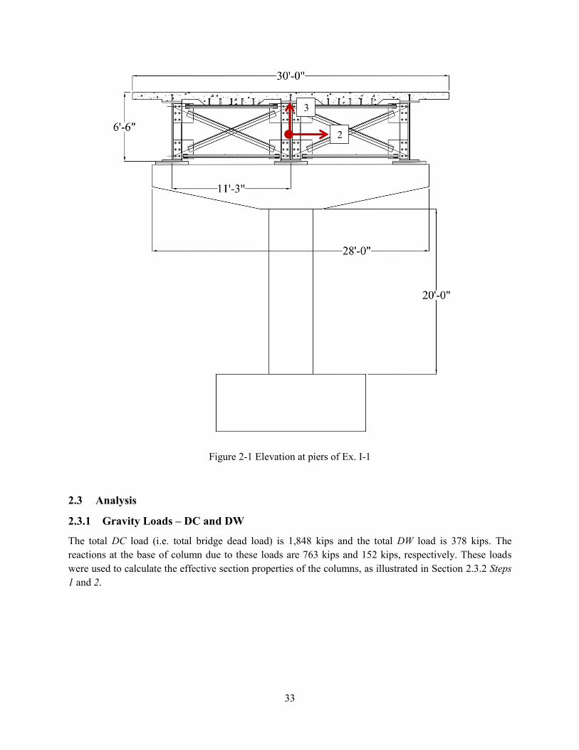
33
Figure 2-1 Elevation at piers of Ex. I-1
2.3 Analysis
2.3.1 Gravity Loads – DC and DW
The total DC load (i.e. total bridge dead load) is 1,848 kips and the total DW load is 378 kips. The
reactions at the base of column due to these loads are 763 kips and 152 kips, respectively. These loads
were used to calculate the effective section properties of the columns, as illustrated in Section 2.3.2 Steps
1 and 2.
2
3

34
Figure 2-2 Analytical model of Ex. I-1
(a) 3D view of model
(b) Detail at piers
(c) Detail at abutments
Beam element located at
superstructure c.g.
Columns and pier cap = beam
element
Link element to
transfer superstructure
vertical and
longitudinal forces to
bearings
x
z
y
Rigid beam element located at deck c.g.
Rigid links to connect rigid
beam element to top chord
Gap link element
Soil link element
Link element for
vertical support only
(i.e. free to translate
in any horizontal
direction)
Cross-frames = beam
elements in elastic
analysis, multi-linear
plastic link elements in
nonlinear analysis.

35
2.3.2 Earthquake Loads – EQ
Step 1: Calculate column axial loads due to
gravity loads, Pcol.
This will be used to determine the effective
moment of inertia, Ie, of the columns.
( ) ( )
Step 2: Determine effective moment of inertia, Ie.
This is accomplished through a section analysis of
the column. The required parameters are: column
diameter, longitudinal and transverse
reinforcements, axial load, and material properties
of the concrete and steel reinforcement.
The calculated Ie is assigned to the beam elements
representing the column in the model.
The following are the column properties:
D = 4 ft
ρl = 1% (12 - #11)
ρs = 1% (#6 @ 4.0 in.)
f‘c = 4 ksi
fy = 60 ksi
Pcol = 1,182 kips
From section analysis:
Ie/Ig = 0.38
Step 3: Estimate soil displacement, Δsoil, and
calculate the effective abutment stiffness, Ke.
The joint gap is included in the calculation of this
stiffness, as shown in the figure below.
Figure 2-3 Abutment force-displacement
The soil passive resistance, Pp, and initial soil
stiffness, Ki, are calculated based on the
recommended values in Caltrans SDC.
( ⁄ ) ( )
( ⁄ ) ( )
where Ae (ft2) is the effective backwall area, h (ft)
is the backwall height, and w is the backwall
Δsoil = 5.01 in.
( )( ⁄ )
( )( ⁄ )
Check Δsoil against Δgap + Δy to determine if the
soil is yielding.
Since this is smaller than Δsoil, the soil is yielding
and the effective stiffness is:

36
width.
Under EQ in the longitudinal direction, only one
abutment is engaged in one direction. To account
for this in the elastic analyses such as modal and
response spectrum analyses, half of Ke is applied
to both abutments.
This 1/2Ke is then distributed to the link elements
representing the soil. The gap link elements shown
in Figure 2-2c were assigned with high stiffness
with no opening during the elastic analysis.
Since there are 6 soil springs at each abutment,
the effective stiffness assigned to each is:
(
)
Step 4: Perform a modal analysis and determine
the required number of modes needed for a
multimode spectral analysis.
After the effective stiffnesses of the elements are
determined, a modal analysis is performed to
determine the fundamental vibration periods and
the required number of modes needed in the
response spectrum analysis. The AASHTO
Specifications require that the total number of
modes used should ensure participation of at least
90% of the total bridge mass.
Table 2-2 shows the result of the modal analysis.
Although only the first 5 modes are shown in this
table, a total of 30 modes were used in the
response spectrum analysis with a total mass
participation of 100% in both the longitudinal
and transverse directions.
The first mode with a period of 2.82 sec is in-
plane deck rotation; the second with a period of
2.23 sec is the transverse translation mode; and
the third with a period of 0.92 sec is the
longitudinal translation mode. The vertical
vibration mode is the fourth mode with a period
of 0.59 sec.
Table 2-2 Modal periods and mass participation
Mode Period Mass Participation
No Sec x-dir y-dir
1 2.82 0.000 0.000
2 2.23 0.000 0.963
3 0.92 0.983 0.000
4 0.59 0.000 0.000
5 0.52 0.000 0.001
Step 5: Perform a response spectrum analysis in
the longitudinal direction (EQx), determine Δsoil,
and check against the initial value in Step 3.
The design spectrum is applied in the longitudinal
direction. Multimode spectral analysis is used and
the modal responses are combined using the
Complete Quadratic Combination (CQC).
From a response spectrum analysis, Δsoil = 5.01
in. Therefore, no further iteration is needed.

37
Step 6: Obtain the column forces due to EQx.
These forces will be combined with the forces due
to EQy to determine the design forces.
Table 2-3 Column forces due to EQx
Load P
(kip)
Mx
(k-ft)
My
(k-ft)
EQx 19 0 4,507
The seismic base shear of the bridge in the
longitudinal direction is 1,285 kips.
Step 7: Perform a response spectrum analysis in
the transverse direction (EQy) and determine the
column forces.
Table 2-4 Column forces due to EQy
Load P
(kip)
Mx
(k-ft)
My
(k-ft)
EQy 0 7,591 0
The seismic base shear of the bridge in the
transverse direction is 524 kips.

38
2.3.3 Design Loads
The 100%-30% combination was used to combine the EQx and EQy forces. The results are shown in
Table 2-5.
Table 2-5 Combination of forces due to EQx and EQy
Load/Combination P
(kip)
Mx
(k-ft)
My
(k-ft)
EQx 19 0 4,507
EQy 0 7,591 0
EQ1: 1.0EQx + 0.3EQy 19 2,277 4,507
EQ2: 0.3EQx + 1.0EQy 6 7,591 1,352
The response modification factor, R, is then applied to the EQ1 and EQ2 column moments. For a bridge
with single-column piers, R for the columns is equal to 3.0. The resulting forces are then combined with
the DC and DW forces to determine the design forces. The load factors are based on the Extreme Event I
load combination and the result is shown in Table 2-6.
Table 2-6 Design loads for columns
Load/Combination P
(kip)
Mx
(k-ft)
My
(k-ft)
DC 763 0 0
DW 152 0 0
EQ1/R 19 759 1,502
EQ2/R 6 2,530 451
LC1: 1.25DC + 1.5DW + 1.0EQ1 1,201 759 1,502
LC2: 1.25DC + 1.5DW + 1.0EQ2 1,188 2,530 451

39
2.4 Design of Columns
Step 1: Determine the design axial load and
resultant moment from Section 2.3.3.
Table 2-7 Design axial load and resultant
moment
Load
Combination
P
(kip)
Mres
(kip-ft)
LC1 1,201 1,683
LC2 1,188 2,570
Step 2: Develop the axial force-moment (P-M)
interaction curve and check if the design loads are
inside the P-M curve.
The AASHTO ϕ factors are used in the interaction
curve.
From the final iteration, the column properties
are:
D = 4 ft
ρl = 1% (12 - #11)
ρs = 1% (#6 @ 4.0 in.)
f‘c = 4 ksi
fy = 60 ksi
The design loads are within the boundaries of the
P-M interaction curve as shown below. Thus, the
selected column size and reinforcement are
adequate.
Step 3: Determine the plastic shear demand, Vp, of
the column.
Vp will be used to design the column transverse
reinforcement and cross-frames. For single-
column piers, Vp is calculated using the equation:
Using the design axial loads in Table 2-7,
determine the nominal moment from the
interaction curve.
for P = 1,201 kips, Mn = 2,977 kip-ft
for P = 1,188 kips Mn = 2,967 kips.
The larger nominal moment is 2,977 kip-ft; thus
it will be used to calculate Vp.
0
1000
2000
3000
4000
5000
0 500 1000 1500 2000 2500 3000
ϕP
n (
kip
)
ϕMn (kip-ft)

40
where Mn is the nominal moment and H is the
height from the base of the column to the
bearings. Mn is determined from the interaction
curve based on the axial load, P, in the column.
Note that the ϕ factors are included in the values
in the interaction curve, thus these values are to be
divided by ϕ to get the nominal values. The 1.3
factor is to account for material overstrength.
( )
Step 4: Determine the column shear demand and
compare against the plastic shear resistance.
The shear resistance can be calculated using the
Simplified Procedure described in AASHTO
Specifications Art. 5.8.3.4.1. For simplicity and
being conservative, the contribution of the
concrete to the shear resistance is not included in
the calculations.
where:
Ash = area of one leg of the transverse
reinforcement; fy is the yield stress of the
transverse reinforcement; s is the spacing of the
transverse reinforcement; D is the diameter of the
column; Dr is the diameter of the circle passing
through the centers of the longitudinal
reinforcement.
The transverse reinforcement is #6 rebar spaced
at 4.0 in. on center. The longitudinal
reinforcement is #11 rebar. The concrete cover is
2.0 in.
( )
( )
( )( )
( )
The demand-resistance ratio is:
Step 5: Check the transverse reinforcement for
confinement
The volumetric ratio of transverse reinforcement
shall satisfy AASHTO Specifications Art.
5.10.11.4.1d:
ρs = 1% (#6 @ 4.0 in.)
fy = 60 ksi
f’c = 4 ksi
(
)

41
The spacing of transverse reinforcement shall
satisfy AASHTO Specifications Art. 5.10.11.4.1e:
,
,
2.5 Seismic Design of Support Cross-Frames
For a Type 1 design strategy, the inelasticity is to be limited in the columns. The components along the
seismic load path, such as the cross-frames, are designed and detailed to remain elastic.
Step 1: Determine the axial force in each of the
cross-frame diagonal members.
where Vp is the column plastic shear, N is the
number of panels, and θ is the angle of the
diagonal member measured from the horizontal.
Vp = 158 kips
N = 2 panels
θ = 26 degrees
( )( )
Step 2: Cross-frame member section properties
Note that the size of the cross-frames may be
governed by slenderness requirements.
Section: L8x8x5/8
Fy = 36 ksi
Ag = 9.61 in2
rx = 2.48 in.
ry = 2.48 in.
rz = 1.58 in.
L = 149.85 in.
Step 3: Calculate the tensile resistance
( )( )
Step 4: Calculate the compressive resistance
Under seismic loading, the cross-frames are
primary members in the transverse direction as
they transmit the deck seismic forces to the
bearings. The actual maximum slenderness ratio is
checked against the limiting slenderness ratio for
primary member which is 120 (AASHTO
( )

42
Specifications Art. 6.9.3).
Equal-leg single angle sections are used as the
diagonal members. The effective slenderness ratio
is calculated according to AASHTO
Specifications Art. 6.9.4.4.
o If l/rx < 80
(
)
o If l/rx > 80
(
)
where rx is the radius of gyration about the
geometric axis of the angle parallel to the
connected leg.
The compressive resistance is then calculated
according to AASHTO Specifications Art. 6.9.2.1,
6.9.4.1.1, and 6.9.4.1.2
(
)
The slender element reduction factor, Q, is equal
to 1.0 when:
√
o If Pe/Po > 0.44
[ ( ⁄ )]
o If Pe/Po < 0.44
( )
Note that although the calculations shown here is
for equal-leg single angle sections for simplicity,
unequal leg single angles and double angles may
l/rx = 149.85/2.48 = 60.42 < 80
(
)
( )
( )
( )
√
( )( )
[ ]( )
The resistance of the selected section, L8x8x5/8,
is much larger than the demand. However, this
section was selected due to the limit on
slenderness ratio.

43
be also used as diagonal members of cross-frames.
Step 5: Calculate the minimum nominal shear
resistance of the cross-frames and check against
Vp of the column.
( )
In this equation, only the nominal compressive
resistance, Pn, is used to determine the minimum
nominal shear resistance and n is the number of
the bays. Note that Pn is smaller than the tensile
resistance, Pr, which means buckling would occur
first in any of the diagonal members before
yielding is reached. Thus, VXF is the minimum
nominal shear force before inelasticity starts to
occur in the cross-frames. Since this is a Type 1
design strategy, Vp should be less than VXF.
(
)
As can be seen above, the slenderness ratio is the
governing parameter in the design of elastic
support cross-frames.

44
2.6 Cross-Frame Properties for Nonlinear Analysis
It is not expected to have inelasticity in the cross-frames when using a Type I design strategy. However,
the expected force and displacement resistances of the cross-frames are calculated for use in the design
evaluation in case inelasticity did occur in the analysis.
Step 1: Calculate the expected tensile yield and
displacement resistance.
The expected yield resistance is:
where Fye is the expected yield stress and is equal
to RyFy. For A36 steel sections, Ry = 1.5.
The effective axial stiffness is:
where E is the modulus of elasticity of steel which
is 29,000 ksi, Ae is the effective area calculated
using Eqn. (1-12), and L is the total length of the
diagonal member.
The expected yield displacement is then calculated
as:
L8x4x3/4
Fye = 1.5(36) = 54 ksi
Ag = 9.61 in2
Ix = 59.6 in4
e = 2.21 in. distance from connected leg of angle
to its c.g.
( )
( )
( )
( )

45
Step 2: Calculate the expected compressive
resistance and associated displacement.
The (Kl/r)eff and Pe are the same as calculated in
Section 2.5 Step 4. The expected yield strength is
used to calculate Po.
The expected compressive resistance is then
calculated as:
o If Pe/Po > 0.44
[ ( ⁄ )]
o If Pe/Po < 0.44
The corresponding displacement is:
( )
( )

46
2.7 Design Summary
The total weight of Ex. I-1 is 1,848 kips. From modal and response spectrum analyses, the periods, forces,
and displacements are:
Parameter Longitudinal Direction Transverse Direction
Fundamental period, T (sec) 0.92 2.23
Base shear, Vb (kip) 1,285 524
Column displacement demand, Δcol (in) 4.60 8.26
Deck displacement demand, Δdeck (in) 4.92 11.58
The column properties are:
Diameter, D 4 ft
Longitudinal reinforcement 12 - #11 (ρl = 1%)
Transverse reinforcement #6 @ 4.0 in. (ρs = 1%)
Effective moment of inertia, Ie 0.38Ig
Plastic shear resistance, Vp 158 kips
The cross-frame diagonal member section properties are:
Section L8x8x5/8 (A36)
Area, A 9.61 in2
Slenderness ratio, KL/r 117.32
Width-thickness ratio, b/t 12.8
Tensile resistance, ϕPr 329 kips
Compressive resistance, ϕPn 151 kips
Min. nominal shear resistance, VXF_min 603 kips
Expected tensile resistance, Pye 519 kips
Expected compression resistance, Pnc 175 kips

47
2.8 Nonlinear Evaluation of Seismic Design
The response under the design earthquake and MCE is discussed in this section.
2.8.1 Response under Design Earthquake
Figure 2-4 shows the column force-displacement plots under the design earthquake. The effective lateral
resistance of the column is 138 kips, calculated from section analysis using the expected material
properties. The column expected yield displacement is 2.42 in. It can be observed in Figure 2-4 that the
displacements in the longitudinal and transverse directions exceeded the yield displacement. However,
yielding in the column was minimal. The average displacement ductility for all runs was 1.7 and the
maximum ductility was 2.8. The negative stiffness that is observed in the hysteresis plots was not due to
instability in the structure or any computational error in the analysis. Rather, it is attributed to the coupled
biaxial response of the column. This phenomenon is observed when the response is elastic and depends
on the frequency content of the input motion and period of the structure (Monzon et al. 2013b).
The cross-frames remained elastic under the design earthquake runs. The maximum total shear force in
the cross-frames was 131 kips. The minimum nominal shear resistance of the cross-frames was 603 kips,
as shown in Section 2.6.
2.8.2 Response under Maximum Considered Earthquake
Figure 2-5 shows the column force-displacement plots under the MCE. There was further inelasticity in
the columns as indicated by the hysteretic response. The average displacement ductility for all runs was
2.3 and the maximum ductility was 3.3.
The support cross-frames also remained elastic at this earthquake level. This is because the shear force in
the transverse direction was limited by the yielding in the columns whose resistance is considerably lower
than the resistance of the cross-frames. The maximum total shear force in the cross-frames was equal to
139 kips.
This evaluation showed that the bridge behaved as designed by limiting the inelasticity to the
substructure. It also showed that the AASHTO Specifications R factor of 3.0 for single column piers is
adequate and conservative for this bridge. The maximum ductility values under the design earthquake and
the MCE were equal to 2.8 and 3.3, respectively, which are close to the R factor used in the design.

48
Longitudinal Direction Transverse Direction
(a) DE1
(b) DE2
(c) DE3
(d) DE4
Figure 2-4 Column force-displacement plots under the design earthquake
-200
-150
-100
-50
0
50
100
150
200
-6 -4 -2 0 2 4 6
Forc
e (
k)
Displacement (in)
-150
-100
-50
0
50
100
150
-6 -4 -2 0 2 4 6
Forc
e (
k)
Displacement (in)
-150
-100
-50
0
50
100
150
-4 -2 0 2 4
Forc
e (
k)
Displacement (in)
-150
-100
-50
0
50
100
150
-8 -4 0 4Fo
rce
(k)
Displacement (in)
-150
-100
-50
0
50
100
150
-4 -2 0 2 4
Forc
e (
k)
Displacement (in)
-150
-100
-50
0
50
100
150
-4 -2 0 2 4
Forc
e (
k)
Displacement (in)
-150
-100
-50
0
50
100
150
-4 -2 0 2 4
Forc
e (
k)
Displacement (in)
-150
-100
-50
0
50
100
150
-4 -2 0 2 4
Forc
e (
k)
Displacement (in)

49
Longitudinal Direction Transverse Direction
(a) MCE1
(b) MCE2
(c) MCE3
(d) MCE4
Figure 2-5 Column force-displacement plots under the MCE
-200
-150
-100
-50
0
50
100
150
200
-6 -2 2 6
Forc
e (
k)
Displacement (in)
-150
-100
-50
0
50
100
150
-6 -2 2 6
Forc
e (k
)
Displacement (in)
-200
-150
-100
-50
0
50
100
150
200
-6 -2 2 6
Forc
e (
k)
Displacement (in)
-200
-150
-100
-50
0
50
100
150
200
-10 -8 -6 -4 -2 0 2 4 6 8Fo
rce
(k)
Displacement (in)
-200
-150
-100
-50
0
50
100
150
-6 -4 -2 0 2 4 6
Forc
e (
k)
Displacement (in)
-150
-100
-50
0
50
100
150
-6 -4 -2 0 2 4 6
Forc
e (
k)
Displacement (in)
-200
-150
-100
-50
0
50
100
150
200
-8 -4 0 4 8
Forc
e (
k)
Displacement (in)
-150
-100
-50
0
50
100
150
-8 -4 0 4 8
Forc
e (
k)
Displacement (in)

50
Chapter 3 Example I-2: Bridge with Single-Column Piers Designed using
the Type 2 Strategy
3.1 Bridge Description
The overall geometry of Ex. I-2 is described in Section 1.3.1. From the final design iteration, the
reinforced concrete (R/C) column diameter is 5 ft-6 in. with 2.1% longitudinal reinforcement and 1%
transverse reinforcement. The pier cap is 6 ft-6 in. wide, and it is tapered with depth starting from 3 ft-4
in. at the ends to 5 ft at the center. Figure 3-1 shows the elevation of Ex. I-2 at the piers. The cross-frames
are an X-type pattern with diagonal members made of L3x3x3/8 single angles, while the top and bottom
chords are 2L2x2x1/4 double angles.
3.2 Computational Model
The computational model is shown in Figure 3-2. The equivalent concrete section properties of the
superstructure are summarized in Table 3-1. The local axes of the superstructure are shown in Figure 3-1.
Deck cracking was approximately accounted for in the calculation of these properties by using 50% of the
gross concrete modulus of elasticity (Ec).
For the elastic analysis, only one of the diagonal members of the cross-frames is included in the model as
shown in Figure 3-2b. This is because the cross-frames are expected to yield and buckle under the design
earthquake. Under transverse loading, in each cross-frame panel, one diagonal is under tension and the
other is in compression. Consequently, the diagonal in compression would buckle and its stiffness
becomes essentially close to zero.
For the nonlinear response history analysis, the cross-frames were modeled with multi-linear plastic link
elements with the force-deformation relationship shown in Figure 1-5. The two cross-frame diagonal
members are modeled because buckling is accounted for in the definition of link force-deformation
relationship. Calculation of the expected forces and deformations is shown in Sections 3.5 and 3.6.
Table 3-1 Ex. I-2 superstructure equivalent concrete section properties
Area, A (in2) 6,028
Moment of inertia about horizontal axis, I2 (in4) 4,660,235
Moment of inertia about vertical axis, I3 (in4) 69,386,665
Torsional constant, J (in4) 102,071

51
Figure 3-1 Elevation at piers of Ex. I-2
3.3 Analysis
3.3.1 Gravity Loads – DC and DW
The total DC load (i.e. total bridge dead load) is 2,014 kips and the total DW load is 378 kips. The
reactions at the base of column due to these loads are 846 kips and 152 kips, respectively. These loads
were used to calculate the effective section properties of the columns, as illustrated in Section 2.3.2 Steps
1 and 2.
2
3

52
Figure 3-2 Analytical model of Ex. I-2
(a) 3D view of model
(b) Detail at piers
(c) Detail at abutments
Beam element located at
superstructure c.g.
Columns and pier cap = beam
element
Link element to
transfer
superstructure
vertical and
longitudinal forces
to bearings
x
z
y
Rigid beam element located at deck c.g.
Rigid links to connect rigid
beam element to top chord
Gap link element
Soil link element
Link element for
vertical support only
(i.e. free to translate
in any horizontal
direction)
Cross-frames = beam
elements in elastic
analysis, multi-linear
plastic link elements in
nonlinear analysis.

53
3.3.2 Earthquake Loads – EQ
Step 1: Calculate the column axial loads due to the
gravity loads, Pcol.
This will be used to determine the effective
moment of inertia, Ie, of the columns.
( ) ( )
Step 2: Determine effective moment of inertia, Ie.
This is accomplished through a section analysis of
the column. The required parameters are: column
diameter, longitudinal and transverse
reinforcements, axial load, and material properties
of the concrete and steel reinforcement.
The calculated Ie is assigned to the beam elements
representing the column in the model.
The following are the column properties:
D = 5.5 ft
ρl = 2.1% (45 - #11)
ρs = 1% (#6 @ 3.0 in.)
f‘c = 4 ksi
fy = 60 ksi
Pcol = 1,286 kips
From section analysis:
Ie/Ig = 0.49
Step 3: Estimate soil displacement, Δsoil, and
calculate the effective abutment stiffness, Ke.
The joint gap is included in the calculation of this
stiffness, as shown in the figure below.
Figure 3-3 Abutment force-displacement
The soil passive resistance, Pp, and initial soil
stiffness, Ki, are calculated based on the
recommended values in Caltrans SDC.
( ⁄ ) ( )
( ⁄ ) ( )
where Ae (ft2) is the effective backwall area, h (ft)
is the backwall height, and w is the backwall
Δsoil = 3.56 in.
( )( ⁄ )
( )( ⁄ )
Check Δsoil against Δgap + Δy to determine if the
soil is yielding.
Since this is smaller than Δsoil, the soil is yielding
and the effective stiffness is:

54
width.
Under EQ in the longitudinal direction, only one
abutment is engaged in one direction. To account
for this in elastic analyses such as modal and
response spectrum analyses, half of Ke is applied
to both abutments.
This 1/2Ke is then distributed to the link elements
representing the soil. The gap link elements shown
in Figure 3-2c were assigned with high stiffness
and no opening during the elastic analysis.
Since there are 6 soil springs at each abutment,
the effective stiffness assigned to each is:
( )
Step 4: Perform a modal analysis and determine
the required number of modes needed for a
multimode spectral analysis.
After the effective stiffnesses of the elements are
determined, a modal analysis is performed to
determine the fundamental vibration periods and
the required number of modes needed in the
response spectrum analysis. The AASHTO
Specifications require that the total number of
modes used should ensure participation of at least
90% of the total bridge mass.
Table 3-2 shows the result of the modal analysis.
Although only the first 5 modes are shown in this
table, a total of 30 modes were used in the
response spectrum analysis with a total mass
participation of 100% in both the longitudinal
and transverse directions.
The first mode with a period of 1.65 sec is in-
plane deck rotation; the second with a period of
1.25 sec is the transverse translation mode; and
the third with a period of 0.64 sec is the
longitudinal translation mode. The vertical
vibration mode is the fourth mode with a period
of 0.58 sec.
The vibration periods in this example are shorter
than those in Ex. I-1 because of the larger
columns.
Table 3-2 Modal periods and mass participation
Mode Period Mass Participation
No Sec x-dir y-dir
1 1.65 0.000 0.000
2 1.27 0.000 0.924
3 0.64 0.969 0.000
4 0.58 0.000 0.000
5 0.51 0.000 0.011
Step 5: Perform a response spectrum analysis in
the longitudinal direction (EQx), determine Δsoil,
and check against the initial value in Step 3.
The design spectrum is applied in the longitudinal
direction. Multimode spectral analysis is used and
the modal responses are combined using the
Complete Quadratic Combination (CQC).
From the response spectrum analysis, Δsoil = 3.47
in. This is within 5% of the assumed
displacement in Step 3, thus no further iteration is
needed.

55
Step 6: Obtain the column forces due to EQx.
These forces will be used to design the columns.
Table 3-3 Column forces due to EQx
Load P
(kip)
Mx
(k-ft)
My
(k-ft)
EQx 0 0 13,010
The seismic base shear of the bridge in the
longitudinal direction is 1,943 kips.
3.3.3 Design Loads
In the Type 2 design strategy, the design loads are from DC, DW, and EQx only. A proposed R factor of
1.5 is applied to EQx forces. The forces based on the Extreme Event I load combination are shown in
Table 3-4.
Table 3-4 Design loads for columns
Load/Combination P
(kip)
Mx
(k-ft)
My
(k-ft)
DC 846 0 0
DW 152 0 0
EQx 0 0 13,010
EQ1 = EQx/R 0 0 8,673
LC1: 1.25DC + 1.5DW + 1.0EQ1 1,286 0 8,673

56
3.4 Design of Columns
Step 1: Determine the design axial load and
resultant moment from Section 3.3.3.
Table 3-5 Design axial load and resultant
moment
Load
Combination
P
(kip)
Mres
(kip-ft)
LC1 1,286 8,673
Step 2: Develop the axial force-moment (P-M)
interaction curve and check if the design loads are
inside the P-M curve.
The AASHTO ϕ factors are used in the interaction
curve.
From the final iteration the column properties
are:
D = 5.5 ft
ρl = 2.1% (45 - #11)
ρs = 1% (#6 @ 3.0 in.)
f‘c = 4 ksi
fy = 60 ksi
The design loads are within the boundaries of the
P-M interaction curve as shown below. Thus, the
selected column size and reinforcement are
adequate.
Step 3: Determine the plastic shear demand, Vp, of
the column.
Vp will be used to design the column transverse
reinforcement and cross-frames. For single-
column piers, Vp is calculated using the equation:
Using the design axial loads in Table 3-5,
determine the nominal moment from the
interaction curve.
for P = 1,286 kips, Mn = 10,230 kip-ft
The nominal moment is 10,230 kip-ft and will be
used to calculate Vp.
0
2000
4000
6000
8000
10000
0 4000 8000 12000
P (
kip
)
Moment (kip-ft)

57
where Mn is the nominal moment and H is the
height from the base of the column to the
bearings. Mn is determined from the interaction
curve based on the axial load, P, in the column.
Note that the ϕ factors are included in the values
in the interaction curve, thus these values are to be
divided by ϕ to get the nominal values. The 1.3
factor is to account for material overstrength.
( )
Step 4: Determine the column shear resistance and
compare against the plastic shear demand.
The shear resistance can be calculated using the
Simplified Procedure described in AASHTO
Specifications Art. 5.8.3.4.1. For simplicity and to
be conservative, the contribution of the concrete to
the shear resistance is not included in the
calculations.
where:
Ash = area of one leg of the transverse
reinforcement; fy is the yield stress of the
transverse reinforcement; s is the spacing of the
transverse reinforcement; D is the diameter of the
column; Dr is the diameter of the circle passing
through the centers of the longitudinal
reinforcement.
The transverse reinforcement is #6 rebar spaced
at 3.0 in. on center. The longitudinal
reinforcement is #11 rebar. The concrete cover is
2.0 in.
( )
( )
( )( )
( )
The demand-resistance ratio is:
Step 5: Check the transverse reinforcement.
The volumetric ratio of transverse reinforcement
shall satisfy AASHTO Specifications Art.
5.10.11.4.1d:
The spacing of transverse reinforcement shall
ρs = 1% (#6 @ 3.0 in.)
fy = 60 ksi
f’c = 4 ksi
(
)

58
satisfy AASHTO Specifications Art. 5.10.11.4.1e:
,
,

59
3.5 Design of Support Ductile End Cross-Frames
In the proposed Type 2 seismic design, the interior support cross-frames are designed such that their
resistance is less than the column nominal shear resistance in the transverse direction so that the
inelasticity will be limited to the cross-frames in that direction.
Step 1: Determine the cross-frame force based on
the nominal shear resistance of the column.
The cross-frame shear force is equal to the
nominal shear resistance of the column in the
transverse direction.
where Vp is the column plastic shear resistance.
The corresponding cross-frame diagonal member
axial force with the R factor applied is:
where n is the number of bays, θ is the angle of
the diagonal from the horizontal, and R is the
cross-frame response modification factor taken
equal to 4.0. In this equation, only one diagonal is
assumed resisting the shear force. This is because,
in a panel, one diagonal is in tension and the other
one is in compression. The compression diagonal
is expected to buckle in which case its post-
buckling resistance is considerably smaller, thus
the resistance is largely due to the yield resistance
of the diagonal in tension.
Vp = 523 kips
n = 2 bays
θ = 26o
( )
Step 2: Determine the cross-frame force from the
response spectrum analysis in the transverse
direction.
Step 3: The design cross-frame force is the
smaller of PXF1 or PXF2.
PXF = 55.95 kips
Step 4: Determine the cross-frame size. A36 single angle

60
The required area is:
where Fy is the nominal yield stress of the cross-
frame. The nominal value is used since PXF was
calculated from the nominal shear force.
Note that the size of the cross-frame may be
governed by the compactness and slenderness
requirements shown in Step 5.
Fy = 36 ksi
Use L3x3x3/8
Ag = 2.11 in2
rz = 0.581 in
I = 1.75 in4
x = 0.884 in. distance from connected leg of
angle to its c.g.
L = 149.85 in
Step 5: Check the compactness and slenderness
ratios.
The diagonal members of ductile cross-frames
shall satisfy proposed AASHTO Specifications
Art. 6.16.4.5.2a:
√
The slenderness ratio shall satisfy proposed
AASHTO Specifications Art. 6.16.4.5.2b:
√
where K is 0.85, l is taken as one-half of the
length of the diagonal member due to biased
buckling, r is the radius of gyration normal to the
plane of buckling and is equal to rz for single
angle members.
√
( )
√
Step 6: Calculate the expected yield resistance.
where Fye is the expected yield stress and is equal
to RyFy. For A36 steel sections, Ry = 1.5.
Fye = 1.5(36) = 54 ksi
( )( )
Step 7: Calculate the expected compressive

61
resistance.
The compressive resistance is calculated
according to AASHTO Specifications Art. 6.9.2.1,
6.9.4.1.1, and 6.9.4.1.2
(
)
o If Pe/Po > 0.44
[ ( ⁄ )]
o If Pe/Po < 0.44
( )
( ) ( )
( )
[ ( )]( )
Step 8: Calculate the maximum expected lateral
resistance of the cross-frames and compare against
the column nominal shear resistance.
The maximum lateral resistance is the maximum
of:
( )
where Pt = 1.2Pye is the tensile resistance of the
diagonal member. The 1.2 factor is to account for
the upper bound of tensile resistance. The 0.3Pnc
term is taken to represent the post-buckling
resistance of the diagonal member. Vlat1 typically
governs particularly with relatively slender
diagonal members. Vlat2 may govern in cases
where the diagonal members are short and stocky.
The cross-frame maximum lateral resistance is
compared against the column nominal shear
resistance to ensure elastic columns.
( )
[ ( )]
[ ( )]
Therefore, Vlat = 270 kips
Step 9: Determine the superstructure drift and
check against limit.
After the cross-frame is designed, the
superstructure drift is determined. The
superstructure lateral displacement is calculated
( )
( )

62
using the equation:
where PEQY is the force in the cross-frame
diagonal member determined from the response
spectrum analysis in the transverse direction and
Ae is the effective area calculated using Eqn.
(1-12).
The superstructure lateral drift should not exceed
4% (proposed AASHTO Specification Art.
6.16.4.5.1).
( )
( )
3.6 Cross-Frame Properties for Nonlinear Analysis
The expected force and displacement resistances of the cross-frames are calculated for use in the design
evaluation.
Step 1: Calculate the expected tensile yield
displacement.
The expected yield resistance is calculated in
Section 3.5 Step 6.
The effective axial stiffness is:
where E is the modulus of elasticity of steel which
is 29,000 ksi, Ae is the effective area calculated
using Eqn. (1-12), and L is the total length of the
diagonal member.
The expected yield displacement is then calculated
as:
L3x3x3/8
Pye = 113.94 kips
Ag = 2.11 in2
I = 1.75 in4
x = 0.884 in. distance from connected leg of
angle to its c.g.
( )
( )
( )
Step 2: Calculate the expected compressive
displacement.
The expected compressive resistance is calculated

63
in Section 3.5 Step 7.
The corresponding displacement is:
Pnc = 44.11 kips
3.7 Design Summary
The total weight of Ex. I-2 is 2,014 kips. The fundamental period in the longitudinal direction is 0.64 sec
and in the transverse direction it is 1.27 sec. The column properties are:
Diameter, D 5.5 ft
Longitudinal reinforcement 45 - #11 (ρl = 2.1%)
Transverse reinforcement #6 @ 3.0 in. (ρs = 1%)
Effective moment of inertia, Ie 0.49Ig
Plastic shear demand, Vp 523 kips
The cross-frame diagonal member section properties are:
Section L3x3x3/8 (A36)
Area, Ag 2.11 in2
Slenderness ratio, KL/r 109.61
Width-thickness ratio, b/t 8.0
Expected tensile yield resistance, Pye 114 kips
Expected compressive resistance, Pnc 44 kips
Lateral resistance of cross-frames, Vlat 270 kips

64
3.8 Nonlinear Evaluation of Seismic Design
The response under the design earthquake and MCE is discussed in this section.
3.8.1 Response under Design Earthquake
Figure 3-4 shows the column force-displacement plots under the design earthquake. The effective lateral
resistance of the column is 478 kips, calculated from the section analysis using expected material
properties. The corresponding expected yield displacement is 1.32 in. There was minimal yielding in the
columns. The average displacement ductility for all runs was 1.2 and the maximum was 1.8. The
inelasticity was concentrated in the cross-frames and thus limited the transverse seismic forces.
The total transverse shear force in the pier bearings plotted against the relative girder displacement is
shown in Figure 3-6. As shown, the cross-frames were yielding under the design earthquake. The average
girder drift was 4.1%.
3.8.2 Response under Maximum Considered Earthquake
The column force-displacement plots are shown in Figure 3-5. Minimum yielding was observed in
columns and they can be considered essentially elastic. The average displacement ductility was 1.4 and
the maximum ductility was 2.3. Figure 3-7 shows the inelastic response of the cross-frames under the
MCE. The average girder drift was 6.4%.
This evaluation showed that the bridge behaved as designed. The inelasticity was concentrated at the
interior-support cross-frames that were designed to withstand this demand. The bridge substructure stayed
essentially elastic even at the MCE-level. This proves that the proposed seismic design procedure for the
Type 2 strategy achieved the intended seismic performance by limiting the inelasticity to the interior-
support cross-frames while keeping the bridge substructure essentially elastic as intended.

65
Longitudinal Direction Transverse Direction
(a) DE1
(b) DE2
(c) DE3
(d) DE4
Figure 3-4 Column force-displacement under the design earthquake
-600
-400
-200
0
200
400
600
-3 -2 -1 0 1 2 3
Shea
r Fo
rce
(ki
p)
Displacement (in)
-400
-300
-200
-100
0
100
200
300
400
-2 -1 0 1 2
Shea
r Fo
rce
(ki
p)
Displacement (in)
-500
-400
-300
-200
-100
0
100
200
300
400
500
-2 -1 0 1 2
Shea
r Fo
rce
(ki
p)
Displacement (in)
-400
-300
-200
-100
0
100
200
300
400
-2 -1 0 1 2
Shea
r Fo
rce
(ki
p)
Displacement (in)
-600
-400
-200
0
200
400
600
-3 -2 -1 0 1 2 3
Shea
r Fo
rce
(ki
p)
Displacement (in)
-400
-300
-200
-100
0
100
200
300
-2 -1 0 1 2
Shea
r Fo
rce
(ki
p)
Displacement (in)
-600
-400
-200
0
200
400
600
-3 -2 -1 0 1 2 3
Shea
r Fo
rce
(ki
p)
Displacement (in)
-300
-200
-100
0
100
200
300
400
-2 -1 0 1 2
Shea
r Fo
rce
(ki
p)
Displacement (in)

66
Longitudinal Direction Transverse Direction
(a) MCE1
(b) MCE2
(c) MCE3
(d) MCE4
Figure 3-5 Column force-displacement under the MCE
-600
-400
-200
0
200
400
600
800
-4 -2 0 2 4
Shea
r Fo
rce
(ki
p)
Displacement (in)
-400
-300
-200
-100
0
100
200
300
400
-3 -2 -1 0 1 2
Shea
r Fo
rce
(ki
p)
Displacement (in)
-500
-400
-300
-200
-100
0
100
200
300
400
500
-3 -2 -1 0 1 2 3
Shea
r Fo
rce
(ki
p)
Displacement (in)
-400
-300
-200
-100
0
100
200
300
400
-3 -2 -1 0 1 2
Shea
r Fo
rce
(ki
p)
Displacement (in)
-600
-400
-200
0
200
400
600
800
-4 -3 -2 -1 0 1 2 3
Shea
r Fo
rce
(ki
p)
Displacement (in)
-500
-400
-300
-200
-100
0
100
200
300
-3 -2 -1 0 1 2 3
Shea
r Fo
rce
(ki
p)
Displacement (in)
-600
-400
-200
0
200
400
600
-3 -2 -1 0 1 2 3
Shea
r Fo
rce
(ki
p)
Displacement (in)
-400
-300
-200
-100
0
100
200
300
400
500
-3 -2 -1 0 1 2
Shea
r Fo
rce
(ki
p)
Displacement (in)

67
(a) DE1 (b) DE2
(c) DE3 (d) DE4
Figure 3-6 Superstructure transverse shear force – displacement under the design earthquake
-300
-200
-100
0
100
200
300
-3 -2 -1 0 1
She
ar F
orc
e (
kip
)
Displacement (in)
-300
-200
-100
0
100
200
300
-2 -1 0 1 2 3
She
ar F
orc
e (
kip
)
Displacement (in)
-300
-200
-100
0
100
200
300
-1 0 1 2 3
She
ar F
orc
e (
kip
)
Displacement (in)
-400
-300
-200
-100
0
100
200
300
-4 -3 -2 -1 0 1
She
ar F
orc
e (
kip
)
Displacement (in)

68
(a) MCE1 (b) MCE2
(c) MCE3 MCE4
Figure 3-7 Superstructure transverse shear force – displacement under the MCE
-400
-300
-200
-100
0
100
200
300
-6 -4 -2 0 2
She
ar F
orc
e (
kip
)
Displacement (in)
-400
-300
-200
-100
0
100
200
300
-6 -4 -2 0 2 4
She
ar F
orc
e (
kip
)
Displacement (in)
-300
-200
-100
0
100
200
300
400
-1 0 1 2 3 4
She
ar F
orc
e (
kip
)
Displacement (in)
-400
-300
-200
-100
0
100
200
300
-6 -4 -2 0 2 4
She
ar F
orc
e (
kip
)
Displacement (in)

69
Chapter 4 Example II-1: Bridge with Two-Column Piers Designed using
the Type 1 Strategy
4.1 Bridge Description
The overall geometry of Ex. II-1 is described in Section 1.3.2. From the final design iteration, the
reinforced concrete (R/C) column diameter is 4 ft with 1% longitudinal steel ratio and 1.4% transverse
steel ratio. The rectangular pier cap is 5 ft wide and 4 ft deep. The pier cap is 60 ft long and the center-to-
center distance between the columns is 40 ft. Figure 4-1 shows the elevation of Ex. II-1 at the piers. The
cross-frames are an X-type pattern with diagonal members made of L8x8x5/8 single angles while the top
and bottom chords are 2L4x4x1/2 double angles.
4.2 Computational Model
The computational model is shown in Figure 4-2. The equivalent concrete section properties of
superstructure are summarized in Table 4-1. The local axes of the superstructure are shown in Figure 4-1.
Deck cracking was approximately accounted for in the calculation of these properties by using 50% of the
gross concrete modulus of elasticity (Ec).
For the nonlinear response history analysis, the cross-frames were modeled with multi-linear plastic link
element with the force-deformation relationship shown in Figure 1-5 to account for inelasticity in case it
occurred. Calculation of the expected force and deformations is shown in Section 4.6.
Table 4-1 Ex.II-1 superstructure section properties
Area, A (in2) 16,195
Moment of inertia about horizontal axis, I2 (in4) 10,316,084
Moment of inertia about vertical axis, I3 (in4) 8.22 x 10
8
Torsional constant, J (in4) 285,124

70
Figure 4-1 Elevation at pier of Ex. II-1
4.3 Analysis
4.3.1 Gravity Loads – DC and DW
The total DC load (i.e. total bridge dead load) is 3,933 kips and the total DW load is 844 kips. The
reactions at the base of each column due to these loads are 801 kips and 166 kips, respectively. These
loads were used to calculate the effective section properties of the columns, as illustrated in Section 4.3.2
Steps 1 and 2.
2
3
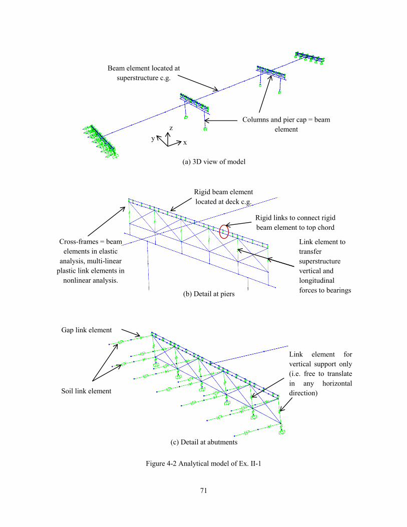
71
Figure 4-2 Analytical model of Ex. II-1
(a) 3D view of model
(b) Detail at piers
(c) Detail at abutments
Beam element located at
superstructure c.g.
Columns and pier cap = beam
element
Link element to
transfer
superstructure
vertical and
longitudinal
forces to bearings
x
z
y
Rigid beam element
located at deck c.g.
Rigid links to connect rigid
beam element to top chord
Gap link element
Soil link element
Link element for
vertical support only
(i.e. free to translate
in any horizontal
direction)
Cross-frames = beam
elements in elastic
analysis, multi-linear
plastic link elements in
nonlinear analysis.

72
4.3.2 Earthquake Loads – EQ
Step 1: Calculate column axial loads due to the
gravity loads, Pcol.
This will be used to determine the effective
moment of inertia, Ie, of columns.
( ) ( )
Step 2: Determine effective moment of inertia, Ie.
This is accomplished through a section analysis of
the column. The required parameters are: column
diameter, longitudinal and transverse
reinforcements, axial load, and material properties
of the concrete and steel reinforcement.
The calculated Ie is assigned to the beam elements
representing the column in the model.
The following are the column properties:
D = 4 ft
ρl = 1% (12 - #11)
ρs = 1.4% (#6 @ 3.0 in.)
f‘c = 4 ksi
fy = 60 ksi
Pcol = 1,250 kips
From section analysis:
Ie/Ig = 0.38
Step 3: Estimate soil displacement, Δsoil, and
calculate the effective abutment stiffness, Ke.
The joint gap is included in the calculation of this
stiffness, as shown in the figure below.
Figure 4-3 Abutment force-displacement
The soil passive resistance, Pp, and initial soil
stiffness, Ki, are calculated based on the
recommended values in Caltrans SDC.
( ⁄ ) ( )
( ⁄ ) ( )
where Ae (ft2) is the effective backwall area, h (ft)
is the backwall height, and w is the backwall
Δsoil = 5.0 in.
( )( ⁄ )
( )( ⁄ )
Check Δsoil against Δgap + Δy to determine if the
soil is yielding.
Since this is smaller than Δsoil, the soil is yielding
and the effective stiffness is:

73
width.
Under EQ in the longitudinal direction, only one
abutment is engaged in one direction. To account
for this in elastic analyses such as modal and
response spectrum analyses, half of Ke is applied
to both abutments.
This 1/2Ke is then distributed to the link elements
representing the soil. The gap link elements shown
in Figure 4-2c were assigned with high stiffness
and no opening during the elastic analysis.
Since there are 12 soil springs at each abutment,
the effective stiffness assigned to each is:
( )
Step 4: Perform modal analysis and determine the
required number of modes needed for a multimode
spectral analysis.
After the effective stiffnesses of the elements are
determined, a modal analysis is performed to
determine the fundamental vibration periods and
the required number of modes needed in the
response spectrum analysis. The AASHTO
Specifications requires that the total number of
modes used should ensure participation of at least
90% of the total bridge mass.
Table 4-2 shows the result of the modal analysis.
Although only the first 5 modes are shown in this
table, a total of 30 modes were used in the
response spectrum analysis with total mass
participation of 100% in both the longitudinal
and transverse directions.
The first mode with a period of 0.94 sec is
longitudinal translation mode; the second with a
period of 0.94 sec is in-plane deck rotation mode;
and the third with a period of 0.68 sec is the
transverse translation mode. The vertical
vibration mode is the fourth mode with a period
of 0.34 sec.
Table 4-2 Modal periods and mass participation
Mode Period Mass Participation
No Sec x-dir y-dir
1 0.94 0.981 0.000
2 0.92 0.000 0.000
3 0.68 0.000 0.980
4 0.34 0.000 0.000
5 0.24 0.000 0.006
Step 5: Perform a response spectrum analysis in
the longitudinal direction (EQx), determine Δsoil,
and check against the initial value in Step 3.
The design spectrum is applied in the longitudinal
direction. Multimode spectral analysis is used and
the modal responses are combined using the
Complete Quadratic Combination (CQC).
From the response spectrum analysis, Δsoil = 5.05
in. Therefore, no further iteration is needed.

74
Step 6: Obtain the column forces due to EQx.
These forces will be combined with the forces due
to EQy to determine the design forces.
Table 4-3 Column forces due to EQx
Load P
(kip)
Mx
(k-ft)
My
(k-ft)
EQx 17 0 5,317
The seismic base shear of the bridge in the
longitudinal direction is 2,676 kips.
Step 7: Perform response spectrum analysis in the
transverse direction (EQy) and determine the
column forces.
Table 4-4 Column forces due to EQy
Load P
(kip)
Mx
(k-ft)
My
(k-ft)
EQy 858 9,369 0
The seismic base shear of the bridge in the
transverse direction is 3,731 kips.

75
4.3.3 Design Loads
The 100%-30% combination was used to combine the EQx and EQy forces. The results are shown in
Table 4-5.
Table 4-5 Combination of forces due to EQx and EQy
Load/Combination P
(kip)
Mx
(k-ft)
My
(k-ft)
EQx 17 0 5,317
EQy 858 9,369 0
EQ1: 1.0EQx + 0.3EQy 274 2,811 5,317
EQ2: 0.3EQx + 1.0EQy 863 9,369 1,595
The response modification factor, R, is then applied to EQ1 and EQ2 moments. For a bridge with multi-
column piers, R for the columns is equal to 5.0. The resulting forces are then combined with the DC and
DW forces to determine the design forces. The load factors are based on the Extreme Event I load
combination and the result is shown in Table 4-6.
Table 4-6 Design loads for columns
Load/Combination P
(kip)
Mx
(k-ft)
My
(k-ft)
DC 801 0 0
DW 166 0 0
EQ1/R 274 562 1,063
EQ2/R 863 1,874 319
LC1: 1.25DC + 1.5DW + 1.0EQ1 1,524 562 1,063
LC2: 1.25DC + 1.5DW + 1.0EQ2 2,113 1,874 319

76
4.4 Design of Columns
Step 1: Determine the design axial load and
resultant moment from Section 4.3.3.
Table 4-7 Design axial load and resultant moment
Load
Combination
P
(kip)
Mres
(kip-ft)
LC1 1,524 1,202
LC2 2,113 1,901
Step 2: Develop the axial force-moment (P-M)
interaction curve and check if the design loads are
inside the P-M curve.
The AASHTO ϕ factors are used in the interaction
curve.
From the final iteration the column properties are:
D = 4 ft
ρl = 1% (12 - #11)
ρs = 1.4% (#6 @ 3.0 in.)
f‘c = 4 ksi
fy = 60 ksi
The design loads are within the boundaries of P-
M interaction curve as shown below. Thus, the
selected column size and reinforcement are
adequate.
Step 3: Determine the plastic shear demand, Fp, of
the piers in transverse direction
The plastic moment resistance, Mp, of column is a
function of its axial load. In a multi-column pier,
due to frame action, there is a variation in the
column axial loads resulting in different plastic
moment capacities. Calculation of Fp is therefore
an iterative process. The calculation of Fp is
0
1000
2000
3000
4000
5000
0 1000 2000 3000
ϕP
n (
kip
)
ϕMn (kip-ft)

77
outlined in the procedure below.
Step 3.1: Start the calculation process by using the
column axial load, P, obtained from LC1.
The following procedure, up to Step 3.7, is
repeated to calculate Fp based on P from LC2. The
maximum Fp calculated from LC1 and LC2 will
be used to design the transverse reinforcement and
cross-frames
Step 3.2: Based on this P, determine Mn from the
interaction curve.
Step 3.3: Determine Mp and Vp.
where the 1.3 factor is to account for column
overstrength.
where H is the column clear height. This equation
is based on double-curvature behavior. This
behavior is typically assumed for a multi-column
pier because the cap beam is much stiffer than the
columns.
Step 3.4: Calculate Fp and ΔP.
The following equations are based on the free-
body diagram for a two-column pier shown in
Figure 4-4.
From Table 4-7, P = 1,524 kips.
Since this P was from a response spectrum
analysis, both columns of the pier have the same
P.
By interpolating on the points of the interaction
curve, Mn = 3,197 kip-ft for P = 1,524 kips.
Mp = 1.3(3,197) = 4,156 kip-ft
Vp = 2(4,156)/20 = 416 kips

78
Figure 4-4 Forces in a two-column pier
( ) ( )
where L is the distance between the two columns.
Step 3.5: Update the axial load in the columns.
Where P1 is the updated axial load in the left
column and Pp is updated axial load in the right
column.
Step 3.6: Update Mn, Mp, and Vp in the columns.
The new plastic moments and shears are
determined using P1 and P2.
Step 3.7: Calculate the new Fp and ΔP and
compare against that in Step 3.4.
Fp = 416 + 416 = 832 kips
( ) ( )
P1 = 1,524 – 208 = 1,315 kips
P2 = 1,524 + 208 = 1,731 kips
For P1 = 1,315 kips
Mn1 = 3,058 kip-ft from interaction curve
Mp1 = 1.3(3,058)= 3,975 kip-ft
Vp1 = 2(3,975)/20 = 398 kips
For P2 = 1,731 kips
Mn2 = 3,324 kip-ft from interaction curve
Mp2 = 1.3(3,324) = 4,321 kip-ft
Vp2 = 2(4,321)/20 = 432 kips
Fp = 398 + 432 = 830 kips
Fp
H
Vp1 Vp2Mp1 Mp1
ΔP ΔP

79
If Fp in this step is within 5% of that in Step 3.4,
further iteration is not necessary. Otherwise,
repeat Steps 3.4 to 3.7.
Step 3.8: Repeat Steps 3.1 to 3.7 using P from
LC2.
Step 3.8: Determine the maximum Fp and the
maximum column plastic shear resistance.
This is the maximum of the results from Steps 3.7
and 3.8. The results will be used to design the
column transverse reinforcement and cross-
frames.
( ) ( )
Since Fp and ΔP are within 5% of the previous
values, further iteration is not necessary.
The calculations were started using P = 2,113
kips from LC2 in Table 4-7. The results of the
last iteration are:
Mp1 = 4,410 kip-ft
Vp1 = 441 kips
Mp2 = 4,571 kip-ft
Vp = 457 kips
Fp = 868 kips
From the results of Steps 3.7 and 3.8:
Vp = 457 kips (maximum Vp per column)
Fp = 868 kips (maximum Fp for the pier)
Step 4: Determine the column shear resistance
and compare against the plastic shear demand.
The shear resistance can be calculated using the
Simplified Procedure described in AASHTO
Specifications Art. 5.8.3.4.1. For simplicity and to
be conservative, the contribution of the concrete
to the shear resistance is not included in the
calculations.
where:
The transverse reinforcement is #6 rebar spaced
at 3.0 in. on center. The longitudinal
reinforcement is #11 rebar. The concrete cover is
2.0 in.
( )
( )

80
Ash = area of one leg of the transverse
reinforcement; fy is the yield stress of the
transverse reinforcement; s is the spacing of the
transverse reinforcement; D is the diameter of the
column; Dr is the diameter of the circle passing
through the centers of the longitudinal
reinforcement.
( )( )
( )
The maximum Vp = 457 kips per column.
The demand-resistance ratio is:
Step 5: Check the transverse reinforcement.
The volumetric ratio of transverse reinforcement
shall satisfy AASHTO Specifications Art.
5.10.11.4.1d:
The spacing of transverse reinforcement shall
satisfy AASHTO Specifications Art. 5.10.11.4.1e:
,
ρs = 1.4% (#6 @ 3.0 in.)
fy = 60 ksi
f’c = 4 ksi
(
)
,

81
4.5 Seismic Design Support of Cross-Frames
For a Type 1 design strategy, the inelasticity is to be limited to the columns. The components along the
seismic load path, such as the cross-frames, are designed and detailed to remain elastic.
Step 1: Determine the axial force in each of the
cross-frame diagonal members.
where Fp is the pier plastic shear resistance, n is
the number of bays, and θ is the angle of the
diagonal member measured from the horizontal.
Vp = 868 kips
n= 5 panels
θ = 22 degrees
( )( )
Step 2: Cross-frame member section properties
Note that the size of the cross-frames may be
governed by slenderness requirements.
Section: L8x8x5/8
Fy = 36 ksi
Ag = 9.61 in2
rx = ry = 2.48 in.
rz = 1.58 in.
L = 142.62 in.
Step 3: Calculate the tensile resistance
( )( )
Step 4: Calculate the compressive resistance
Under seismic loading, the cross-frames are
primary members in the transverse direction as
they transmit the deck seismic forces to the
bearings. The actual maximum slenderness ratio is
checked against the limiting slenderness ratio for
primary member which is 120 (AASHTO
Specifications Art. 6.9.3).
Equal-leg single angle sections are used as the
diagonal members. The effective slenderness ratio
is calculated according to AASHTO
Specifications Art. 6.9.4.4.
o If l/rx < 80
( )
l/rx = 142.62/2.48 = 57.51 < 80

82
(
)
o If l/rx > 80
(
)
The compressive resistance is calculated
according to AASHTO Specifications Art. 6.9.2.1,
6.9.4.1.1, and 6.9.4.1.2
(
)
The slender element reduction factor, Q, is equal
to 1.0 when:
√
o If Pe/Po > 0.44
[ ( ⁄ )]
o If Pe/Po < 0.44
( )
Note that although the calculations shown here is
for single angle sections, unequal-leg single
angles and double angles may be also used as
diagonal members of cross-frames.
(
)
( )
( )
( )
√
( )( )
[ ]( )
The resistance of the selected section, L8x8x5/8,
is much larger than the demand. However, this
section was selected due to the limit on
slenderness ratio.
Step 5: Calculate the minimum nominal shear
resistance of the cross-frames and check against
Vp of the column.
( )
In this equation, only the compression resistance,
Pn, is used to determine the minimum nominal
shear resistance. Note that Pn is smaller than the
(
)

83
tension resistance, Pr, which means buckling
would occur first in any of the diagonal members
before yielding is reached. Thus, VXF is the
minimum shear force before inelasticity starts to
occur in the cross-frames. Since this is a Type 1
design – inelasticity is accommodated in the
columns only – Vp should be less thanVXF.
As can be seen above, the slenderness ratio is the
governing parameter in the design of elastic
support cross-frames.
4.6 Cross-Frame Properties for Nonlinear Analysis
The expected force and displacement resistances of the cross-frames are calculated for use in the design
evaluation.
Step 1: Calculate the expected tensile yield and
displacement resistance.
The expected yield resistance is:
where Fye is the expected yield stress and is equal
to RyFy. For A36 steel sections, Ry = 1.5.
The effective axial stiffness is:
where E is the modulus of elasticity of steel which
is 29,000 ksi, Ae is the effective area calculated
using Eqn. (1-12), and L is the total length of the
diagonal member.
The expected yield displacement is then calculated
as:
L8x8x5/8
Fye = 1.5(36) = 54 ksi
Ag = 9.61 in2
I = 59.6 in4
e = 2.21 in. distance from connected leg of angle
to its c.g.
( )
( )
( )
( )
Step 2: Calculate the expected compressive
resistance and associated displacement.
The (Kl/r)eff and Pe are the same as that calculated
in Section 4.5 Step 4. The expected yield strength
is used to calculate Po.
The expected compressive resistance is then
( )

84
calculated as:
o If Pe/Po > 0.44
[ ( ⁄ )]
o If Pe/Po < 0.44
The corresponding displacement is:
( )
4.7 Design Summary
The total weight of Ex. II-1 is 3,933 kips. From modal and response spectrum analyses, the periods,
forces, and displacements are:
Parameter Longitudinal Direction Transverse Direction
Fundamental period, T (sec) 0.94 0.68
Base shear, Vb (kip) 2,676 3,731
Column displacement demand, Δcol (in) 3.73 3.17
Pier base shear demand, Fb (kip) 450 1,866
Deck displacement demand, Δdeck (in) 5.06 3.37
The column properties are:
Diameter, D 4 ft
Longitudinal reinforcement 12 - #11 (ρl = 1%)
Transverse reinforcement #6 @ 3.0 in. (ρs = 1.4%)
Effective moment of inertia, Ie 0.38Ig
Column plastic shear resistance, Vp 457 kips
Pier plastic shear resistance, Fp 898 kips
The cross-frame diagonal member section properties are:
Section L8x8x5/8 (A36)
Area, A 9.61 in2
Slenderness ratio, KL/r 115.13
Width-thickness ratio, b/t 12.8

85
Tensile resistance, ϕPr 329 kips
Compressive resistance, ϕPn 155 kips
Min. nominal shear resistance, VXF_min 1,597 kips
Expected tensile yield resistance, Pye 519 kips
Expected compressive resistance, Pnc 182 kips
4.8 Performance Assessment
The response under the design earthquake and MCE is discussed in this section.
4.8.1 Response under Design Earthquake
In the longitudinal direction, the columns deflect in single-curvature and the effective lateral resistance
per column is 146 kips. In the transverse direction, the columns deflect in double-curvature and the
effective yield shear resistance per column is 358 kips. Therefore, the effective yield shear resistances per
pier are 292 and 716 kips in the longitudinal and transverse directions, respectively. The corresponding
yield displacements are 2.32 in. and 1.06 in., respectively. These resistances and displacements were
calculated from the expected material properties of the column.
Figure 4-5 shows the pier force-displacement plots under the design earthquake. This is the sum of the
column shear forces plotted against the displacement at top of the column in the longitudinal and
transverse directions. More inelasticity is observed in the transverse direction than in the longitudinal
direction. This is because the transverse direction is stiffer; thus, it attracks more seismic forces in this
direction. The maximum displacement ductility in the longitudinal direction was 1.8 while in the
transverse direction the maximum displacement ductility was 3.6.
The cross-frames remained elastic in all the design earthquake runs. The maximum total shear force in the
cross-frames is 895 kips. The minimum nominal shear resistance of the cross-frames is 1,597 kips, as
shown in Section 4.5 Step 5.
4.8.2 Response under Maximum Considered Earthquake
Figure 4-6 shows the pier force-displacement plots under the MCE. Although there is an apparent
inelasticity increase in the longitudinal direction, yielding is still considered minimal since the average
ductility was 2.1 and the maximum ductility was only 2.3. In the transverse direction, yielding of the
columns is more pronounced with an average displacement ductility in this direction was 3.9 and the
maximum displacement ductility was 5.1.
The cross-frames remained elastic under the MCE as the maximum total shear force in the cross-frames is
979 kips which is well below their resistance.
This nonlinear evaluation showed that the bridge behaved as designed by limiting the inelasticity to the
substructure. It also showed that the AASHTO Specifications R factor for a two-column pier is adequate
for this bridge since the maximum ductility values under the design earthquake and the MCE were equal
to 3.6 and 5.1, respectively, which are close to the R factor used in the seismic design.

86
Longitudinal Direction Transverse Direction
(a) DE1
(b) DE2
(c) DE3
-400
-300
-200
-100
0
100
200
300
400
-6 -4 -2 0 2 4 6
Forc
e (k
)
Displacement (in)
-1000
-800
-600
-400
-200
0
200
400
600
800
1000
-3 -2 -1 0 1 2 3
Forc
e (k
)
Displacement (in)
-400
-300
-200
-100
0
100
200
300
-4 -2 0 2 4
Forc
e (k
)
Displacement (in)
-1000
-800
-600
-400
-200
0
200
400
600
800
1000
-4 -2 0 2 4
Forc
e (k
)
Displacement (in)
-400
-300
-200
-100
0
100
200
300
-6 -4 -2 0 2 4
Forc
e (k
)
Displacement (in)
-1000
-800
-600
-400
-200
0
200
400
600
800
-3 -2 -1 0 1 2
Forc
e (k
)
Displacement (in)
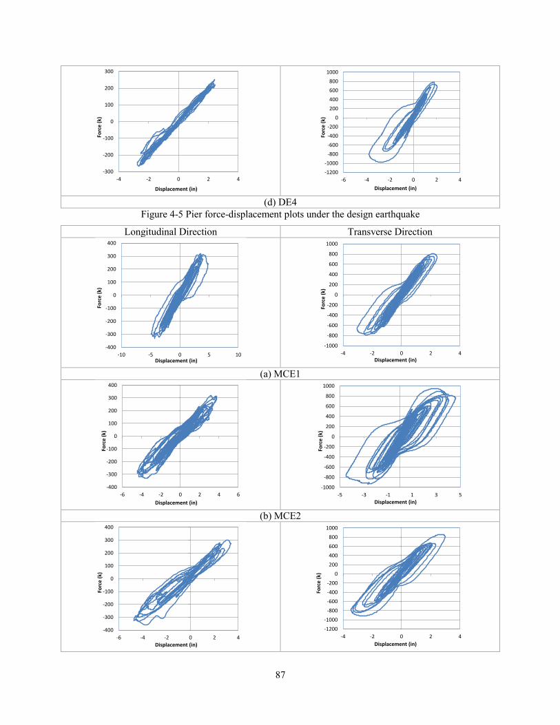
87
(d) DE4
Figure 4-5 Pier force-displacement plots under the design earthquake
Longitudinal Direction Transverse Direction
(a) MCE1
(b) MCE2
-300
-200
-100
0
100
200
300
-4 -2 0 2 4
Forc
e (k
)
Displacement (in)
-1200
-1000
-800
-600
-400
-200
0
200
400
600
800
1000
-6 -4 -2 0 2 4
Forc
e (k
)
Displacement (in)
-400
-300
-200
-100
0
100
200
300
400
-10 -5 0 5 10
Forc
e (k
)
Displacement (in)
-1000
-800
-600
-400
-200
0
200
400
600
800
1000
-4 -2 0 2 4
Forc
e (k
)
Displacement (in)
-400
-300
-200
-100
0
100
200
300
400
-6 -4 -2 0 2 4 6
Forc
e (k
)
Displacement (in)
-1000
-800
-600
-400
-200
0
200
400
600
800
1000
-5 -3 -1 1 3 5
Forc
e (k
)
Displacement (in)
-400
-300
-200
-100
0
100
200
300
400
-6 -4 -2 0 2 4
Forc
e (k
)
Displacement (in)
-1200
-1000
-800
-600
-400
-200
0
200
400
600
800
1000
-4 -2 0 2 4
Forc
e (k
)
Displacement (in)

88
(c) MCE3
(d) MCE4
Figure 4-6 Pier force-displacement plots under the MCE
-400
-300
-200
-100
0
100
200
300
400
500
-10 -5 0 5 10
Forc
e (k
)
Displacement (in)
-1500
-1000
-500
0
500
1000
-6 -4 -2 0 2 4
Forc
e (k
)
Displacement (in)

89
Chapter 5 Example II-2: Bridge with Two-Column Piers Designed using
the Type 2 Strategy
5.1 Bridge Description
The overall geometry of Ex. II-2 is described in Section 1.3.2. From the final design iteration, the
reinforced concrete (R/C) column diameter is 5 ft-6in. with 2.8% longitudinal steel ratio and 2.6%
transverse steel ratio. The rectangular pier cap is 6 ft-6in. wide and 5 ft-6 in. deep. The pier cap is 60 ft
long and the center-to-center distance between the columns is 40 ft. Figure 5-1 shows the elevation of Ex.
II-2 at the piers. The cross-frames are an X-type pattern with diagonal members made of L4x4x1/2 single
angles while the top and bottom chords are 2L2x2x1/4 double angles.
5.2 Computational Model
The computational model is shown in Figure 5-2. The equivalent concrete section properties of
superstructure are summarized in Table 5-1. The local axes of the superstructure are shown in Figure 5-1.
Deck cracking was approximately accounted for in the calculation of these properties by using 50% of the
gross concrete modulus of elasticity (Ec).
For elastic analysis, only one of the diagonal members of the cross-frames is included in the model as
shown in Figure 5-2b. This is because the cross-frames are designed and detailed to yield and buckle
under the design earthquake. Under transverse loading, in each cross-frame panel, one diagonal is under
tension and the other is in compression. Consequently, the diagonal in compression would buckle and its
stiffness becomes essentially zero.
For nonlinear response history analysis, the cross-frames were modeled with multi-linear plastic link
elements with the force-deformation relationship shown in Figure 1-5. The two cross-frame diagonal
members are modeled because buckling is accounted for in the definition of link force-deformation
relationship. Calculation of the expected force and deformations is shown in Sections 5.5 and 5.6.
Table 5-1 Ex.II-1 superstructure section properties
Area, A (in2) 16,195
Moment of inertia about horizontal axis, I2 (in4) 10,316,084
Moment of inertia about vertical axis, I3 (in4) 8.22 x 10
8
Torsional constant, J (in4) 285,124

90
Figure 5-1 Elevation at pier of Ex. II-2
5.3 Analysis
5.3.1 Gravity Loads – DC and DW
The total DC load (i.e. total bridge dead load) is 3,933 kips and the total DW load is 844 kips. The
reactions at the base of each column due to these loads are 904 kips and 166 kips, respectively. These
loads were used to calculate the effective section properties of the columns, as illustrated in Section 5.3.2
Steps 1 and 2.
2
3

91
Figure 5-2 Analytical model of Ex. II-2
(a) 3D view of model
(b) Detail at piers
(c) Detail at abutments
Beam element located at
superstructure c.g.
Columns and pier cap = beam
element
Link element
to transfer
superstructure
vertical and
longitudinal
forces to
bearings
x
z
y
Rigid beam element
located at deck c.g.
Rigid links to connect rigid
beam element to top chord
Gap link element
Soil link element
Link element for
vertical support only
(i.e. free to translate
in any horizontal
direction)
Cross-frames = beam
elements in elastic analysis,
multi-linear plastic link
elements in nonlinear
analysis.

92
5.3.2 Earthquake Loads – EQ
Step 1: Calculate column axial loads due to the
gravity loads, Pcol.
This will be used to determine the effective
moment of inertia, Ie, of the columns.
( ) ( )
Step 2: Determine effective moment of inertia, Ie.
This is accomplished through a section analysis of
the column. The required parameters are: column
diameter, longitudinal and transverse
reinforcements, axial load, and material properties
of the concrete and steel reinforcement.
The calculated Ie is assigned to the beam elements
representing the column in the model.
The following are the column properties:
D = 5.5 ft
ρl = 2.8% (66 - #11)
ρs = 2.6% (#8 @ 2.0 in.)
f‘c = 4 ksi
fy = 60 ksi
Pcol = 1,379 kips
From section analysis:
Ie/Ig = 0.57
Step 3: Estimate soil displacement, Δsoil, and
calculate the effective abutment stiffness, Ke.
The joint gap is included in the calculation of this
stiffness, as shown in the figure below.
Figure 5-3 Abutment force-displacement
The soil passive resistance, Pp, and initial soil
stiffness, Ki, are calculated based on the
recommended values in Caltrans SDC.
( ⁄ ) ( )
( ⁄ ) ( )
where Ae (ft2) is the effective backwall area, h (ft)
is the backwall height, and w is the backwall
Δsoil = 3.3 in.
( )( ⁄ )
( )( ⁄ )
Check Δsoil against Δgap + Δy to determine if the
soil is yielding.
Since this is smaller than Δsoil, the soil is yielding
and the effective stiffness is:

93
width.
Under EQ in the longitudinal direction, only one
abutment is engaged in one direction. To account
for this in elastic analyses such as modal and
response spectrum analyses, half of Ke is applied
to both abutments.
This 1/2Ke is then distributed to the link elements
representing the soil. The gap link elements shown
in Figure 5-2c were assigned with high stiffness
and no opening during the elastic analysis.
Since there are 12 soil springs at each abutment,
the effective stiffness assigned to each is:
( )
Step 4: Perform a modal analysis and determine
the required number of modes needed for
multimode spectral analysis.
After the effective stiffnesses of the elements are
determined, a modal analysis is performed to
determine the fundamental vibration periods and
the required number of modes needed in the
response spectrum analysis. The AASHTO
Specifications requires that the total number of
modes used should ensure participation of at least
90% of the total bridge mass.
Table 5-2 shows the result of the modal analysis.
Although only the first 5 modes are shown in this
table, a total of 30 modes were used in the
response spectrum analysis with a total mass
participation of 100% in both the longitudinal
and transverse directions.
The first mode with a period of 0.64 sec is in-
plane deck rotation; the second with a period of
0.61 sec is the longitudinal translation mode; the
third with a period of 0.57 sec is the vertical
vibration mode; and the fourth with a period of
0.48 sec is the longitudinal translation mode.
The vibration periods in this example are shorter
than those in Ex. II-1 because of the larger
columns.
Table 5-2 Modal periods and mass participation
Mode Period Mass Participation
No Sec x-dir y-dir
1 0.64 0.000 0.000
2 0.61 0.967 0.000
3 0.57 0.000 0.000
4 0.48 0.000 0.887
5 0.34 0.000 0.000
Step 5: Perform a response spectrum analysis in
the longitudinal direction (EQx), determine Δsoil,
and check against the initial value in Step 3.
The design spectrum is applied in the longitudinal
direction. Multimode spectral analysis is used and
the modal responses are combined using the
Complete Quadratic Combination (CQC).
From the response spectrum analysis, Δsoil = 3.26
in. This is within 5% of the assumed
displacement in Step 3, thus no further iteration is
needed.

94
Step 6: Obtain the column forces due to EQx.
These forces will be used to design the columns.
Table 5-3 Column forces due to EQx
Load P
(kip)
Mx
(k-ft)
My
(k-ft)
EQx 0 0 16,255
The seismic base shear in the longitudinal
direction is 4,399 kips.
5.3.3 Design Loads
In the Type 2 design strategy, the design loads are from DC, DW, and EQx only. A proposed R factor of
1.5 is applied to EQx forces. The forces based on the Extreme Event I load combination are shown in
Table 5-4.
Table 5-4 Design loads for columns
Load/Combination P
(kip)
Mx
(k-ft)
My
(k-ft)
DC 904 0 0
DW 166 0 0
EQx 0 0 16,255
EQ1 = EQx/R 0 0 10,837
LC1: 1.25DC + 1.5DW + 1.0EQ1 1,379 0 10,837

95
5.4 Design of Columns
Step 1: Determine the design axial load and
resultant moment from Section 5.3.3.
Table 5-5 Design axial load and resultant moment
Load
Combination
P
(kip)
Mres
(kip-ft)
LC1 1,379 10,837
Step 2: Develop the axial force-moment (P-M)
interaction curve and check if the design loads are
inside the P-M curve.
The AASHTO ϕ factors are used in the interaction
curve.
From the final iteration the column properties are:
D = 5.5 ft
ρl = 2.8% (61 - #11)
ρs = 2.6% (#8 @ 2.0 in.)
f‘c = 4 ksi
fy = 60 ksi
The design loads are within the boundaries of P-
M interaction curve as shown below. Thus, the
selected column size and reinforcement are
adequate.
Step 3: Determine the plastic shear demand, Fp, of
the piers in transverse direction
The plastic moment resistance, Mp, of column is a
function of its axial load. In multi-column pier,
due to frame action, there is variation in column
axial loads resulting in different plastic moment
capacities. Calculation of Fp is therefore an
iterative process. The calculation of Fp is outlined
in the procedure below.
0
2000
4000
6000
8000
10000
12000
0 4000 8000 12000
ϕP
n (
kip
)
ϕMn (kip-ft)

96
Step 3.1: Start the calculation process by using the
column axial load, P, obtained from LC1.
Step 3.2: Based on this P, determine Mn from the
interaction curve.
Step 3.3: Determine Mp and Vp.
where the 1.3 factor is to account for column
overstrength.
where H is the column clear height. This equation
is based on double-curvature behavior. This
behavior is typically assumed for a multi-column
pier because the cap beam is much stiffer than the
columns.
Step 3.4: Calculate Fp and ΔP.
The following equations are based on the free-
body diagram for a two-column pier shown in
Figure 5-4.
Figure 5-4 Forces in a two-column pier
From Table 5-5, P = 1,379 kips.
Since this P was from response spectrum
analysis, both columns of the pier have the same
P.
By interpolating on the points of the interaction
curve, Mn = 12,633 kip-ft for P = 1,379 kips.
Mp = 1.3(12,633) = 16,423 kip-ft
Vp = 2(16,423)/20 = 1,642 kips
Fp
H
Vp1 Vp2Mp1 Mp1
ΔP ΔP

97
( ) ( )
where L is the distance between the two columns.
Step 3.5: Update the axial load in the columns.
Where P1 is the updated axial load in left column
and Pp is updated axial load in right column.
Step 3.6: Update Mn, Mp, and Vp in the columns.
The new plastic moments and shears are
determined using P1 and P2.
Step 3.7: Calculate the new Fp and ΔP and
compare against that in Step 3.4.
If Fp in this step is within 5% of that in Step 3.4,
further iteration is not necessary. Otherwise,
repeat Steps 3.4 to 3.7.
Fp = 1,642 + 1,642 = 3,284 kips
( ) ( )
P1 = 1,379 – 821 = 558 kips
P2 = 1,379 + 821 = 2,200 kips
For P1 = 558 kips
Mn1 = 11,806 kip-ft from interaction
curve
Mp1 = 1.3(11,806)= 15,348 kip-ft
Vp1 = 2(15,348)/20 = 1,535 kips
For P2 = 2,200 kips
Mn2 = 13,283 kip-ft from interaction
curve
Mp2 = 1.3(13,283) = 17,268 kip-ft
Vp2 = 2(17,268)/20 = 1,727 kips
Fp = 1,535 + 1,727 = 3,262 kips
( ) ( )
Since Fp and ΔP are within 5% of previous,
further iteration is not necessary.
Therefore,
Vp = 1,727 kips (maximum Vp per column)
Fp = 3,262 kips (Fp for the pier)

98
Step 4: Determine the column shear resistance
and compare against the plastic shear demand.
The shear resistance can be calculated using the
Simplified Procedure described in AASHTO
Specifications Art. 5.8.3.4.1. For simplicity and
being conservative, the contribution of the
concrete to the shear resistance is not included in
the calculations.
where:
Ash = area of one leg of the transverse
reinforcement; fy is the yield stress of the
transverse reinforcement; s is the spacing of the
transverse reinforcement; D is the diameter of the
column; Dr is the diameter of the circle passing
through the centers of the longitudinal
reinforcement.
The transverse reinforcement is #8 rebar spaced
at 2.0 in. on center. The longitudinal
reinforcement is #11 rebar. The concrete cover is
2.0 in.
( )
( )
( )( )
( )
The maximum Vp = 1,727 kips per column.
The demand-resistance ratio is:
Step 5: Check the transverse reinforcement for
confinement
The volumetric ratio of transverse reinforcement
shall satisfy AASHTO Specifications Art.
5.10.11.4.1d:
The spacing of transverse reinforcement shall
satisfy AASHTO Specifications Art. 5.10.11.4.1e:
,
ρs = 2.6% (#8 @ 2.0 in.)
fy = 60 ksi
f’c = 4 ksi
(
)
,

99
5.5 Design of Support Ductile Cross-Frames
In the proposed Type 2 seismic design, the interior cross-frames are designed such that their resistance is
less than the column nominal shear resistance in the transverse direction so that the inelasticity will be
limited to the cross-frames in that direction.
Step 1: Determine the cross-frame force based on
nominal shear resistance of the pier.
The cross-frame shear force is equal to the
nominal shear resistance of the pier in the
transverse direction.
where Fp is the pier plastic shear resistance.
The corresponding cross-frame diagonal member
axial force with R factor applied is:
where n is the number of bays, θ is the angle of
the diagonal from the horizontal, and R is the
cross-frame response modification factor taken
equal to 4.0. In this equation, only one diagonal is
assumed resisting the shear force. This is because,
in a panel, one diagonal is in tension and the other
one is in compression. The compression diagonal
is expected to buckle in which case its post-
buckling resistance is considerably smaller, thus
the resistance is largely due to the yield resistance
of the diagonal in tension.
Fp = 3,262 kips
n = 5
θ = 22o
( )
Step 2: Determine the cross-frame force from the
response spectrum analysis in the transverse
direction.
Step 3: The design cross-frame force is the
smaller of PXF1 or PXF2.
PXF = 135.31 kips
Step 4: Determine the cross-frame size. A36 single angle

100
The required area is:
where Fy is the nominal yield stress of the cross-
frame. The nominal value is used since PXF was
calculated from the nominal shear force.
Note that the size of the cross-frame may be
governed by the compactness and slenderness
requirements shown in Step 5.
Fy = 36 ksi
Use L4x4x1/2
Ag = 3.75 in2
rz = 0.776 in
I = 5.52 in4
x = 1.18 in. distance from connected leg of angle
to its c.g.
L = 142.62 in
Step 5: Check the compactness and slenderness
ratios.
The diagonal members of ductile cross-frames
shall satisfy (proposed AASHTO Specifications
Art. 6.16.4.5.2a):
√
The slenderness ratio shall satisfy proposed
AASHTO Specifications Art. 6.16.4.5.2b:
√
where K is 0.85, l is taken as one-half of the
length of the diagonal member due to biased
buckling, r is the radius of gyration normal to the
plane of buckling and is equal to rz for single
angle members.
√
( )
√
Step 6: Calculate the expected yield resistance.
where Fye is the expected yield stress and is equal
to RyFy. For A36 steel sections, Ry = 1.5.
Fye = 1.5(36) = 54 ksi
( )( )
Step 7: Calculate the expected compressive

101
resistance.
The compressive resistance is calculated
according to AASHTO Specifications Art. 6.9.2.1,
6.9.4.1.1, and 6.9.4.1.2
(
)
o If Pe/Po > 0.44
[ ( ⁄ )]
o If Pe/Po < 0.44
( )
( ) ( )
( )
[ ( )]( )
Step 8: Calculate the maximum expected lateral
resistance of the cross-frames and compare against
the pier nominal shear resistance.
The maximum lateral resistance is the maximum
of:
( )
where Pt = 1.2Pye is the tensile resistance of the
diagonal member. The 1.2 factor is to account for
the upper bound of tensile resistance. The 0.3Pnc
term is taken to represent the post-buckling
resistance of the diagonal member. Vlat1 typically
governs particularly with relatively slender
diagonal members. Vlat2 may govern in cases
where the diagonal members are short and stocky.
The cross-frame maximum lateral resistance is
compared against the pier nominal shear
resistance to ensure elastic columns.
( )
[ ( )]
[ ( )]
Therefore, Vlat = 1,301 kips
Step 9: Determine the superstructure drift and
check against limit.
After the cross-frame is designed, the
superstructure drift is determined. The
( )
( )
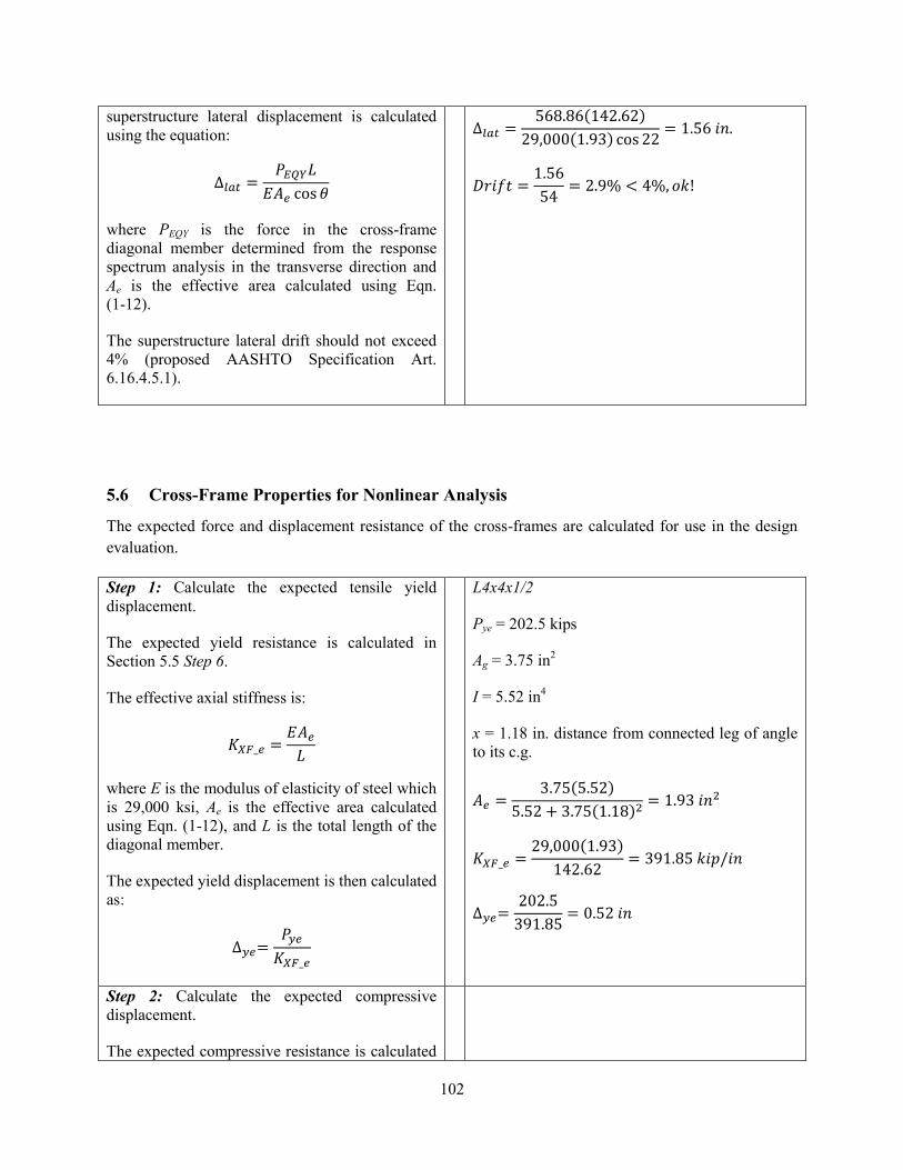
102
superstructure lateral displacement is calculated
using the equation:
where PEQY is the force in the cross-frame
diagonal member determined from the response
spectrum analysis in the transverse direction and
Ae is the effective area calculated using Eqn.
(1-12).
The superstructure lateral drift should not exceed
4% (proposed AASHTO Specification Art.
6.16.4.5.1).
( )
( )
5.6 Cross-Frame Properties for Nonlinear Analysis
The expected force and displacement resistance of the cross-frames are calculated for use in the design
evaluation.
Step 1: Calculate the expected tensile yield
displacement.
The expected yield resistance is calculated in
Section 5.5 Step 6.
The effective axial stiffness is:
where E is the modulus of elasticity of steel which
is 29,000 ksi, Ae is the effective area calculated
using Eqn. (1-12), and L is the total length of the
diagonal member.
The expected yield displacement is then calculated
as:
L4x4x1/2
Pye = 202.5 kips
Ag = 3.75 in2
I = 5.52 in4
x = 1.18 in. distance from connected leg of angle
to its c.g.
( )
( )
( )
Step 2: Calculate the expected compressive
displacement.
The expected compressive resistance is calculated
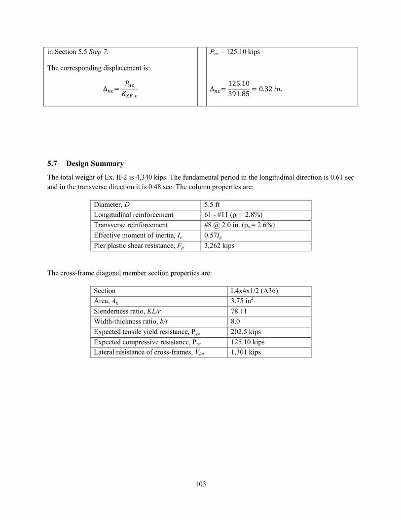
103
in Section 5.5 Step 7.
The corresponding displacement is:
Pnc = 125.10 kips
5.7 Design Summary
The total weight of Ex. II-2 is 4,340 kips. The fundamental period in the longitudinal direction is 0.61 sec
and in the transverse direction it is 0.48 sec. The column properties are:
Diameter, D 5.5 ft
Longitudinal reinforcement 61 - #11 (ρl = 2.8%)
Transverse reinforcement #8 @ 2.0 in. (ρs = 2.6%)
Effective moment of inertia, Ie 0.57Ig
Pier plastic shear resistance, Fp 3,262 kips
The cross-frame diagonal member section properties are:
Section L4x4x1/2 (A36)
Area, Ag 3.75 in2
Slenderness ratio, KL/r 78.11
Width-thickness ratio, b/t 8.0
Expected tensile yield resistance, Pye 202.5 kips
Expected compressive resistance, Pnc 125.10 kips
Lateral resistance of cross-frames, Vlat 1,301 kips
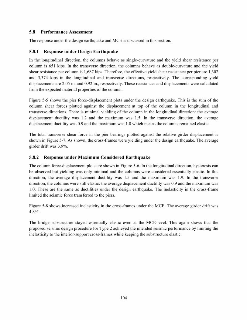
104
5.8 Performance Assessment
The response under the design earthquake and MCE is discussed in this section.
5.8.1 Response under Design Earthquake
In the longitudinal direction, the columns behave as single-curvature and the yield shear resistance per
column is 651 kips. In the transverse direction, the columns behave as double-curvature and the yield
shear resistance per column is 1,687 kips. Therefore, the effective yield shear resistance per pier are 1,302
and 3,374 kips in the longitudinal and transverse directions, respectively. The corresponding yield
displacements are 2.05 in. and 0.92 in., respectively. These resistances and displacements were calculated
from the expected material properties of the column.
Figure 5-5 shows the pier force-displacement plots under the design earthquake. This is the sum of the
column shear forces plotted against the displacement at top of the column in the longitudinal and
transverse directions. There is minimal yielding of the column in the longitudinal direction: the average
displacement ductility was 1.2 and the maximum was 1.5. In the transverse direction, the average
displacement ductility was 0.9 and the maximum was 1.0 which means the columns remained elastic.
The total transverse shear force in the pier bearings plotted against the relative girder displacement is
shown in Figure 5-7. As shown, the cross-frames were yielding under the design earthquake. The average
girder drift was 3.9%.
5.8.2 Response under Maximum Considered Earthquake
The column force-displacement plots are shown in Figure 5-6. In the longitudinal direction, hysteresis can
be observed but yielding was only minimal and the columns were considered essentially elastic. In this
direction, the average displacement ductility was 1.5 and the maximum was 1.9. In the transverse
direction, the columns were still elastic: the average displacement ductility was 0.9 and the maximum was
1.0. These are the same as ductilities under the design earthquake. The inelasticity in the cross-frame
limited the seismic force transferred to the piers.
Figure 5-8 shows increased inelasticity in the cross-frames under the MCE. The average girder drift was
4.8%.
The bridge substructure stayed essentially elastic even at the MCE-level. This again shows that the
proposed seismic design procedure for Type 2 achieved the intended seismic performance by limiting the
inelasticity to the interior-support cross-frames while keeping the substructure elastic.

105
Longitudinal Direction Transverse Direction
(a) DE1
(b) DE2
(c) DE3
(d) DE4
Figure 5-5 Column force-displacement under the design earthquake
-1500
-1000
-500
0
500
1000
1500
-4 -2 0 2 4
Forc
e (k
)
Displacement (in)
-2000
-1500
-1000
-500
0
500
1000
1500
2000
2500
-1 -0.5 0 0.5 1
Forc
e (k
)
Displacement (in)
-1500
-1000
-500
0
500
1000
1500
-2 -1 0 1 2
Forc
e (k
)
Displacement (in)
-2000
-1500
-1000
-500
0
500
1000
1500
2000
2500
-1 -0.5 0 0.5 1
Forc
e (k
)
Displacement (in)
-1500
-1000
-500
0
500
1000
1500
-4 -2 0 2 4
Forc
e (k
)
Displacement (in)
-2000
-1500
-1000
-500
0
500
1000
1500
2000
2500
-1 -0.5 0 0.5 1
Forc
e (k
)
Displacement (in)
-1500
-1000
-500
0
500
1000
1500
-3 -2 -1 0 1 2 3
Forc
e (k
)
Displacement (in)
-2000
-1500
-1000
-500
0
500
1000
1500
2000
-1 -0.5 0 0.5 1
Forc
e (k
)
Displacement (in)

106
Longitudinal Direction Transverse Direction
(a) MCE1
(b) MCE2
(c) MCE3
(d) MCE4
Figure 5-6 Column force-displacement under the MCE
-1500
-1000
-500
0
500
1000
1500
2000
-6 -4 -2 0 2 4
Forc
e (k
)
Displacement (in)
-2000
-1500
-1000
-500
0
500
1000
1500
2000
2500
-1 -0.5 0 0.5 1
Forc
e (k
)
Displacement (in)
-1500
-1000
-500
0
500
1000
1500
-3 -2 -1 0 1 2 3
Forc
e (k
)
Displacement (in)
-2500
-2000
-1500
-1000
-500
0
500
1000
1500
2000
2500
-1 -0.5 0 0.5 1
Forc
e (k
)
Displacement (in)
-1500
-1000
-500
0
500
1000
1500
-4 -2 0 2 4
Forc
e (k
)
Displacement (in)
-2000
-1500
-1000
-500
0
500
1000
1500
2000
2500
-1.5 -1 -0.5 0 0.5 1
Forc
e (k
)
Displacement (in)
-1500
-1000
-500
0
500
1000
1500
-4 -2 0 2 4
Forc
e (k
)
Displacement (in)
-2000
-1500
-1000
-500
0
500
1000
1500
2000
-1 -0.5 0 0.5 1
Forc
e (k
)
Displacement (in)

107
(a) DE1 (b) DE2
(c) DE3 (d) DE4
Figure 5-7 Superstructure transverse shear force – displacement under the design earthquake
(a) MCE1 (b) MCE2
(c) MCE3 MCE4
Figure 5-8 Superstructure transverse shear force – displacement under the MCE
-2000
-1500
-1000
-500
0
500
1000
1500
-2 -1.5 -1 -0.5 0 0.5
She
ar F
orc
e (
kip
)
Displacement (in)
-2000
-1500
-1000
-500
0
500
1000
1500
-3 -2 -1 0 1
Shea
r Fo
rce
(kip
)
Displacement (in)
-2000
-1500
-1000
-500
0
500
1000
1500
2000
-3 -2 -1 0 1
Shea
r Fo
rce
(kip
)
Displacement (in)
-2000
-1500
-1000
-500
0
500
1000
1500
2000
-1 0 1 2 3
Shea
r Fo
rce
(kip
)
Displacement (in)
-2000
-1500
-1000
-500
0
500
1000
1500
2000
-3 -2 -1 0 1 2
Shea
r Fo
rce
(kip
)
Displacement (in)
-2000
-1500
-1000
-500
0
500
1000
1500
2000
-4 -3 -2 -1 0 1 2
Shea
r Fo
rce
(kip
)
Displacement (in)
-2000
-1500
-1000
-500
0
500
1000
1500
2000
-3 -2 -1 0 1 2
Shea
r Fo
rce
(kip
)
Displacement (in)
-2000
-1500
-1000
-500
0
500
1000
1500
2000
-2 -1 0 1 2 3
Shea
r Fo
rce
(kip
)
Displacement (in)

108
Chapter 6 Example III-1: Bridge with Wall Piers Designed using the
Type 1 Strategy
6.1 Bridge Description
The overall geometry of Ex. III-1 is described in Section 1.3.3. From the final design iteration, the
reinforced concrete (R/C) wall pier is 40 ft wide and 4 ft thick. The vertical and horizontal steel
reinforcement ratios are both 0.69% (#9 spaced at 6 in.). Figure 6-1 shows the elevation at piers. The
cross-frames are of X-type pattern with diagonal members made of L8x8x1 single angles while the top
and bottom chords are 2L4x4x1/2 double angles.
6.2 Computational Model
The extruded view of the computational model is shown in Figure 6-2 and details of the model are shown
in Figure 6-3. The equivalent concrete section properties of superstructure are summarized in Table 6-1.
The local axes of the superstructure are shown in Figure 6-1. Deck cracking was accounted for in an
approximate fashion in the calculation of these properties by using 50% of the gross concrete modulus of
elasticity (Ec).
The wall pier was modeled as a vertical beam element as shown in Figure 6-3a. The top of wall is then
connected to a horizontal rigid beam element where the link elements representing the bearings are
connected as shown in Figure 6-3b. To ensure correct modeling of the boundary condition at the top of
the wall, the nodes of the horizontal beam element are assigned with rigid constraint such that there is no
relative deformation and rotation between them.
For the nonlinear response history analysis, the cross-frames were modeled with multi-linear plastic link
element with the force-deformation relationship shown in Figure 1-5 to account for inelasticity in case it
occurred. Calculation of the expected forces and deformations is shown in Section 6.6.
Table 6-1 Ex.II-1 superstructure section properties
Area, A (in2) 16,195
Moment of inertia about horizontal axis, I2 (in4) 10,316,084
Moment of inertia about vertical axis, I3 (in4) 8.22 x 10
8
Torsional constant, J (in4) 285,124

109
Figure 6-1 Elevation at pier of Ex. III-1
Figure 6-2 Extruded view of analytical model of Ex. III-1
2
3

110
Figure 6-3 Analytical model of Ex. III-1
(a) 3D view of model
(b) Detail at piers
(c) Detail at abutments
Beam element located at
superstructure c.g.
Walls and pier cap = beam
element
Link element to
transfer
superstructure
vertical and
longitudinal
forces to bearings
x
z y
Rigid beam element
located at deck c.g.
Rigid links to connect rigid
beam element to top chord
Gap link element
Soil link element
Link element for
vertical support only
(i.e. free to translate
in any horizontal
direction)
Cross-frames =
beam elements in
elastic analysis,
multi-linear plastic
link elements in
nonlinear analysis.
Rigid beam element
located at on top
ofwall Nodes along the top of wall are
assigned with rigid constraints

111
6.3 Analysis
6.3.1 Gravity Loads – DC and DW
The total DC load (i.e. total bridge dead load) is 4,704 kips and the total DW load is 844 kips. The
reactions at the base of wall due to these loads are 1,991 kips and 332 kips, respectively. These loads were
used to calculate the effective section properties, as illustrated in Section 6.3.2 Steps 1 and 2.
6.3.2 Earthquake Loads – EQ
Step 1: Calculate wall axial loads due to gravity
loads, Pcol.
This will be used to determine the effective
moment of inertia, Ie, of the pier wall.
( ) ( )
Step 2: Determine effective moment of inertia, Ie.
This is accomplished through a section analysis of
the wall. The required parameters are: wall
dimensions, longitudinal and transverse
reinforcements, axial load, and material properties
of the concrete and steel reinforcement.
The calculated Ie is assigned to the beam elements
representing the wall pier in the model.
The following are the pier wall properties:
w = 40 ft
t = 4 ft
ρv = 0.69% (#9 at 6 in. both face for a total of 158
- #9)
ρh = 0.69% (#9 @ 6 in.)
f’c = 4 ksi
fy = 60 ksi
Pcol = 2,787 kips
From section analysis:
Ie/Ig = 0.24
Step 3: Estimate the soil displacement, Δsoil, and
calculate the effective abutment stiffness, Ke.
The joint gap is included in the calculation of this
stiffness, as shown in the figure below.
Δsoil = 3.75 in.
( )( ⁄ )
( )( ⁄ )
Check Δsoil against Δgap + Δy to determine if the
soil is yielding.

112
Figure 6-4 Abutment force-displacement
The soil passive resistance, Pp, and initial soil
stiffness, Ki, are calculated based on the
recommended values in Caltrans SDC.
( ⁄ ) ( )
( ⁄ ) ( )
where Ae (ft2) is the effective backwall area, h (ft)
is the backwall height, and w is the backwall
width.
Under EQ in the longitudinal direction, only one
abutment is engaged in one direction. To account
for this in the elastic analyses such as modal and
response spectrum analyses, half of Ke is applied
to both abutments.
This 1/2Ke is then distributed to the link elements
representing the soil. The gap link elements shown
in Figure 6-3c were assigned with high stiffness
with no opening during elastic analysis.
Since this is smaller than Δsoil, the soil is yielding
and the effective stiffness is:
Since there are 12 soil springs at each abutment,
the effective stiffness assigned to each is:
( )
Step 4: Perform a modal analysis and determine
the required number of modes needed for
multimode spectral analysis.
After the effective stiffnesses of the elements are
determined, a modal analysis is performed to
determine the fundamental vibration periods and
the required number of modes needed in the
response spectrum analysis. The AASHTO
Specifications requires that the total number of
modes used should ensure participation of at least
90% of the total bridge mass.
Table 6-2 shows the result of the modal analysis.
Although only the first 7 modes are shown in this
table, a total of 30 modes were used in the
response spectrum analysis with total mass
participation of 100% in both the longitudinal
and transverse directions.
The first mode with period of 0.67 sec is
longitudinal translation mode; the second with a
period of 0.57 sec is the vertical vibration mode;
the transverse translation modes are the fifth and
seventh modes with periods of 0.30 sec and 0.17
sec, respectively.
Table 6-2 Modal periods and mass participation
Mode Period Mass Participation
No Sec x-dir y-dir
1 0.67 0.900 0.000
2 0.57 0.000 0.000
3 0.35 0.000 0.000
4 0.34 0.000 0.000
5 0.30 0.000 0.420
6 0.29 0.000 0.000
7 0.17 0.000 0.390

113
Step 5: Perform a response spectrum analysis in
the longitudinal direction (EQx), determine Δsoil,
and check against the initial value in Step 3.
The design spectrum is applied in the longitudinal
direction. Multimode spectral analysis is used and
the modal responses are combined using the
Complete Quadratic Combination (CQC).
From a response spectrum analysis, Δsoil = 3.72
in. This is within less than 5% of the assumed
value, thus, no further iteration is needed.
Step 6: Obtain the column forces due to EQx.
These forces will be combined with the forces due
to EQy to determine the design forces.
Table 6-3 Column forces due to EQx
Load P
(kip)
Fx
(kip)
Fy
(kip)
Mx
(k-ft)
My
(k-ft)
EQx 37 1,136 0 0 27,326
The seismic base shear of the bridge in the
longitudinal direction is 4,014 kips.
Step 7: Perform a response spectrum analysis in
the transverse direction (EQy) and determine the
column forces.
Table 6-4 Column forces due to EQy
Load P
(kip)
Fx
(kip)
Fy
(kip) Mx
(k-ft)
My
(k-ft)
EQy 0 0 2,548 75,952 0
The seismic base shear of the bridge in the
transverse direction is 5,095 kips.

114
6.3.3 Design Loads
The 100%-30% combination was used to combine the EQx and EQy forces. The results are shown in
Table 6-5.
Table 6-5 Combination of forces due to EQx and EQy
Load/Combination P
(kip)
Fx
(kip)
Fy
(kip)
Mx
(k-ft)
My
(k-ft)
EQx 37 1,136 0 0 27,326
EQy 0 0 2,548 75,952 0
EQ1: 1.0EQx + 0.3EQy 37 1,136 764 22,786 27,326
EQ2: 0.3EQx + 1.0EQy 11 341 2,548 75,952 8,198
The response modification factor, R, is then applied to EQ1 and EQ2 moments. The piers are designed as
wall in both directions thus R is equal to 2.0. The resulting forces are then combined with the DC and DW
forces to determine the design forces. The load factors are based on the Extreme Event I load combination
and the result is shown in Table 6-6.
Table 6-6 Design loads
Load/Combination P
(kip)
Fx
(kip)
Fy
(kip)
Mx
(k-ft)
My
(k-ft)
DC 1,991 0 0 0 0
DW 332 0 0 0 0
EQ1/R 37 568 382 11,393 13,663
EQ2/R 11 171 1,274 37,976 4,099
LC1: 1.25DC + 1.5DW + 1.0EQ1 3,024 568 382 11,393 13,663
LC2: 1.25DC + 1.5DW + 1.0EQ2 2,998 171 1,274 37,976 4,099

115
6.4 Design of Wall Pier
Step 1: Determine the design axial load and
resultant moment from Section 6.3.3.
Table 6-7 Design axial load and resultant moment
Load
Comb.
P
(kip)
Mx
(kip-ft)
My
(kip-ft)
Mres
(kip-ft)
LC1 3,024 11,393 13,663 17,790
LC2 2,998 37,976 4,099 38,197
Step 2: Develop the axial force-moment (P-M)
interaction curve and check if the design loads are
inside the P-M curve.
The AASHTO ϕ factors are used in the interaction
curve.
Since the pier is rectangular, an interaction curve
needs to be developed for each load combination.
From the final iteration the wall properties are:
w = 40 ft
t = 4 ft
ρv = 0.69% (#9 @ 6 in. = 158 - #8) vertical reinf.
ρh = 0.69% (#9 @ 6 in.) horizontal reinf.
f’c = 4 ksi
fy = 60 ksi
For LC1:
The interaction curve for θ = 40o is:
0
10000
20000
30000
40000
50000
60000
0 100000 200000 300000 400000
ϕP
n (
kip
)
ϕMn (kip-ft)
P-M curve @ 40 deg for LC1
Mx = 11,393 kip-ft
My = 13,663 kip-ft
θ = 40o
Mres = 17,790 kip-ft

116
Since the design of the wall section is governed
by the forces in the weak axis direction, the
capacity in this direction is also checked against
the forces due to the earthquake in the
longitudinal direction EQx.
For LC2:
The interaction curve for θ = 84o is:
For EQx:
P = 3,024
My = 13,663 kip-ft (R = 2)
The interaction curve for θ = 0o is:
Therefore, the selected section and its
reinforcement are adequate.
Step 3: Determine the shear resistance in the
transverse direction.
The transverse direction is the strong direction of
the wall.
ρh = 0.0069
b = 48 in.
d = 472 in.
0
10000
20000
30000
40000
50000
60000
0 50000 100000 150000 200000 250000 300000 350000ϕ
Pn
(k
ip)
ϕMn (kip-ft)
P-M curve @ 84 deg for LC2
0
10000
20000
30000
40000
50000
60000
0 10000 20000 30000 40000 50000
ϕP
n (
kip
)
ϕMn (kip-ft)
P-M curve @ 0 deg for EQx
Mx = 37,976 kip-ft
My = 4,099 kip-ft
θ = 84o
Mres = 38,197 kip-ft

117
The factored shear resistance, Vr, of the wall pier
is taken as the lesser of (AASHTO Specifications
Art. 5.10.11.4.2):
√ and
* √ +
where ρh is the horizontal steel reinforcement
ratio.
√ ( )( )
[ √ ( )]( )( )
Therefore, Vr = 11,011 kips
The maximum shear demand is 1,274 kips from
Table 6-6.
Step 5: Check the vertical and horizontal
reinforcements.
The minimum vertical and horizontal
reinforcement ratio shall satisfy (AASHTO
Specifications Art. 5.10.11.4.2):
The spacing of vertical and horizontal
reinforcement shall satisfy (AASHTO
Specifications Art. 5.10.11.4.2):

118
6.5 Seismic Design of Support Cross-Frames
Step 1: Determine the design cross-frame force.
Designing the cross-frames based on the shear
resistance of the wall pier may result in large
uneconomical sections due to the large shear
resistance of the wall piers. Therefore, in this case,
the diagonal member design force is taken as the
lesser of:
( )
and
where n is the number of bays, θ is the angle of
the diagonal member measured from the
horizontal, and PEQY is the force in the diagonal
member from the response spectrum analysis in
the transverse direction.
Vr = 11,011 kips
n = 5 bays
θ = 22 degrees
( )( )
From response spectrum analysis in the
transverse direction:
Therefore, the design axial load in the diagonal
member is:
Step 2: Cross-frame member section properties.
Note that the size of the cross-frames may be
governed by slenderness requirements.
Section: L8x8x1
Fy = 36 ksi
Ag = 15.0 in2
rx = ry = 2.43 in.
rz = 1.56 in.
L = 142.62 in.
Step 3: Calculate the tensile resistance
( )( )
Step 4: Calculate the compressive resistance
Under seismic loading, the cross-frames are
primary members in the transverse direction as
they transmit the deck seismic forces to the
bearings. The actual maximum slenderness ratio is
checked against the limiting slenderness ratio for
primary member which is 120 (AASHTO
Specifications Art. 6.9.3).
( )

119
Equal-leg single angle sections are used as the
diagonal members. The effective slenderness ratio
is calculated according to AASHTO
Specifications Art. 6.9.4.4.
o If l/rx < 80
(
)
o If l/rx > 80
(
)
The compressive resistance is calculated
according to AASHTO Specifications Art. 6.9.2.1,
6.9.4.1.1, and 6.9.4.1.2
( )
The slender element reduction factor, Q, is equal
to 1.0 when:
√
o If Pe/Po > 0.44
[ ( ⁄ )]
o If Pe/Po < 0.44
( )
Note that although the calculations shown here are
for single angle sections, double angles may be
also used as diagonal members of cross-frames
under the Type 1 design strategy.
l/rx = 142.62/2.43 = 58.69 < 80
(
)
( )
( )
( )
√
( )( )
[ ]( )
Step 5: Calculate the minimum nominal shear
resistance of the cross-frames

120
( )
In this equation, only the compression resistance,
Pn, is used to determine the minimum nominal
shear resistance. Note that Pn is smaller than the
tensile resistance, Pr, which means buckling
would occur first in any of the diagonal members
before yielding is reached. Thus, VXF is the
minimum shear force before inelasticity starts to
occur in the cross-frames.
Although this is Type 1 design strategy, VXF may
be less than shear resistance of the wall pier. As
noted in Step 1, in cases where the pier shear
resistance is very large, the cross-frames are
designed based on the response spectrum analysis.
This means that the cross-frames may become
inelastic before the shear resistance of the pier is
reached.
(
)
This is less than the nominal shear resistance of
the wall pier:
6.6 Cross-Frame Properties for Nonlinear Analysis
The expected force and displacement resistances of the cross-frames are calculated for use in the design
evaluation.
Step 1: Calculate the expected tensile yield and
displacement resistance.
The expected yield resistance is:
where Fye is the expected yield stress and is equal
to RyFy. For A36 steel sections, Ry = 1.5.
The effective axial stiffness is:
where E is the modulus of elasticity of steel which
is 29,000 ksi, Ae is the effective area calculated
using Eqn. (1-12), and L is the total length of the
diagonal member.
L8x8x1
Fye = 1.5(36) = 54 ksi
Ag = 15.0 in2
I = 89.1 in4
x = 2.40 in. distance from connected leg of angle
to its c.g.
( )
( )
( )
( )

121
The expected yield displacement is then calculated
as:
Step 2: Calculate the expected compressive
resistance and associated displacement.
The (Kl/r)eff and Pe are the same as calculated in
Section 6.5 Step 4. The expected yield strength is
used to calculate Po.
The expected compressive resistance is then
calculated as:
o If Pe/Po > 0.44
[ ( ⁄ )]
o If Pe/Po < 0.44
The corresponding displacement is:
( )( )
( )
6.7 Design Summary
The total weight of Ex. III-1 is 4,383 kips. From modal and response spectrum analyses, the periods,
forces, and displacements are:
Parameter Longitudinal Direction Transverse Direction
Fundamental period, T (sec) 0.91 0.31
Base shear, Vb (kip) 2,877 5,151
Pier displacement, Δpier (in) 4.76 0.21
Pier Base Shear, Fb (kip) 544 2,576
Deck displacement, Δdeck (in) 4.94 0.61
The wall pier properties are:
Width, w 40 ft
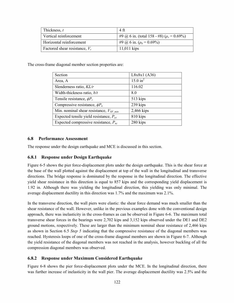
122
Thickness, t 4 ft
Vertical reinforcement #9 @ 6 in. (total 158 - #8) (ρv = 0.69%)
Horizontal reinforcement #9 @ 6 in. (ρh = 0.69%)
Factored shear resistance, Vr 11,011 kips
The cross-frame diagonal member section properties are:
Section L8x8x1 (A36)
Area, A 15.0 in2
Slenderness ratio, KL/r 116.02
Width-thickness ratio, b/t 8.0
Tensile resistance, ϕPr 513 kips
Compressive resistance, ϕPn 239 kips
Min. nominal shear resistance, VXF_min 2,466 kips
Expected tensile yield resistance, Pye 810 kips
Expected compressive resistance, Pnc 280 kips
6.8 Performance Assessment
The response under the design earthquake and MCE is discussed in this section.
6.8.1 Response under Design Earthquake
Figure 6-5 shows the pier force-displacement plots under the design earthquake. This is the shear force at
the base of the wall plotted against the displacement at top of the wall in the longitudinal and transverse
directions. The bridge response is dominated by the response in the longitudinal direction. The effective
yield shear resistance in this direction is equal to 857 kips and the corresponding yield displacement is
1.92 in. Although there was yielding the longitudinal direction, this yielding was only minimal. The
average displacement ductility in this direction was 1.7% and the maximum was 2.1%.
In the transverse direction, the wall piers were elastic: the shear force demand was much smaller than the
shear resistance of the wall. However, unlike in the previous examples done with the conventional design
approach, there was inelasticity in the cross-frames as can be observed in Figure 6-6. The maximum total
transverse shear forces in the bearings were 2,702 kips and 3,152 kips observed under the DE1 and DE2
ground motions, respectively. These are larger than the minimum nominal shear resistance of 2,466 kips
as shown in Section 6.5 Step 5 indicating that the compressive resistance of the diagonal members was
reached. Hysteresis loops of one of the cross-frame diagonal members are shown in Figure 6-7. Although
the yield resistance of the diagonal members was not reached in the analysis, however buckling of all the
compression diagonal members was observed.
6.8.2 Response under Maximum Considered Earthquake
Figure 6-8 shows the pier force-displacement plots under the MCE. In the longitudinal direction, there
was further increase of inelasticity in the wall pier. The average displacement ductility was 2.5% and the
123
maximum was 3.2%. This evaluation showed that the AASHTO Specifications response modification
factor for bridges with wall piers is adequate for this bridge since the maximum displacement ductilities
under the design earthquake and the MCE are close to the R factor used in the seismic design.
In the transverse direction, the shear force demand is still well below the wall shear resistance. There was
further inelasticity in the cross-frames as shown in Figure 6-9. The maximum total transverse shear forces
in the bearings were 3,527 kips and 3,779 kips observed under the MCE1 and MCE2 ground motions,
respectively. Hysteresis loops in Figure 6-10 show that the diagonal members in the support cross-frames
have buckled.
This evaluation showed that the cross-frames in bridges with stiff substructures may become inelastic
even though they are designed using the Type 1 strategy. This is due to the large shear resistance of the
wall pier in the transverse direction such that the support cross-frames yield before the yield shear
resistance of the piers is reached. In this case, preventing the support cross-frames from going nonlinear
may result in an uneconomical section. Bridge designers should be cautioned about this finding since the
connections of the cross frames and the bearings are not designed as capacity protected for this failure
mode.

124
Longitudinal Direction Transverse Direction
(a) DE1
(b) DE2
Figure 6-5 Wall pier force-displacement under the design earthquake
(a) DE1 (b) DE2
Figure 6-6 Superstructure transverse shear force – displacement under the design earthquake
(a) DE1 (b) DE2
Figure 6-7 Hysteresis loops in one of the cross-frame diagonal members under the design earthquake
-1000
-500
0
500
1000
1500
-6 -4 -2 0 2 4
Shea
r Fo
rce
(ki
p)
Displacement (in)
-4000
-3000
-2000
-1000
0
1000
2000
3000
-0.2 -0.1 0 0.1 0.2
Shea
r Fo
rce
(ki
p)
Displacement (in)
-800
-600
-400
-200
0
200
400
600
800
-3 -2 -1 0 1 2 3
Shea
r Fo
rce
(ki
p)
Displacement (in)
-4000
-3000
-2000
-1000
0
1000
2000
3000
4000
-0.2 -0.1 0 0.1 0.2 0.3
Shea
r Fo
rce
(ki
p)
Displacement (in)
-3000
-2000
-1000
0
1000
2000
3000
-0.3 -0.2 -0.1 0 0.1 0.2 0.3
She
ar F
orc
e (
kip
)
Displacement (in)
-3000
-2000
-1000
0
1000
2000
3000
4000
-0.4 -0.2 0 0.2 0.4
She
ar F
orc
e (
kip
)
Displacement (in)
-400
-300
-200
-100
0
100
200
300
-0.3 -0.2 -0.1 0 0.1 0.2
Axi
al F
orc
e (
kip
)
Deformation (in)
-400
-300
-200
-100
0
100
200
300
400
-0.3 -0.2 -0.1 0 0.1 0.2 0.3
Axi
al F
orc
e (
kip
)
Deformation (in)

125
Longitudinal Direction Transverse Direction
(a) MCE1
(b) MCE2
Figure 6-8 Wall pier force-displacement under the MCE
-2000
-1000
0
1000
2000
3000
4000
-10 -5 0 5 10
Shea
r Fo
rce
(ki
p)
Displacement (in)
-4000
-3000
-2000
-1000
0
1000
2000
3000
4000
5000
-0.3 -0.2 -0.1 0 0.1 0.2 0.3
Shea
r Fo
rce
(ki
p)
Displacement (in)
-1200
-1000
-800
-600
-400
-200
0
200
400
600
800
1000
-4 -2 0 2 4
Shea
r Fo
rce
(ki
p)
Displacement (in)
-5000
-4000
-3000
-2000
-1000
0
1000
2000
3000
4000
5000
-0.3 -0.2 -0.1 0 0.1 0.2 0.3
Shea
r Fo
rce
(ki
p)
Displacement (in)

126
(a) MCE1 (b) MCE2
Figure 6-9 Superstructure transverse shear force – displacement under the MCE
(a) MCE1 (b) MCE2
Figure 6-10 Hysteresis loops in one of the support cross-frame diagonal members under the MCE
-4000
-3000
-2000
-1000
0
1000
2000
3000
4000
-0.4 -0.2 0 0.2 0.4 0.6
She
ar F
orc
e (
kip
)
Displacement (in)
-4000
-3000
-2000
-1000
0
1000
2000
3000
4000
5000
-0.6 -0.4 -0.2 0 0.2 0.4 0.6 0.8
She
ar F
orc
e (
kip
)
Displacement (in)
-400
-300
-200
-100
0
100
200
300
400
500
-0.4 -0.3 -0.2 -0.1 0 0.1 0.2 0.3
Axi
al F
orc
e (
kip
)
Deformation (in)
-400-300-200-100
0100200300400500600700
-0.6 -0.4 -0.2 0 0.2 0.4
Axi
al F
orc
e (
kip
)
Deformation (in)

127
Chapter 7 Example III-2: Bridge with Wall Piers Designed using the
Type 2 Strategy
7.1 Bridge Description
The overall geometry of Ex. III-2 is described in Section 1.3.3. From the final design iteration, the
reinforced concrete (R/C) wall pier is 40 ft wide and 4 ft thick. The vertical and horizontal steel
reinforcement ratios are both 0.69% (#9 spaced at 6 in.). Figure 7-1 shows the elevation of Ex. III-2 at the
piers. The cross-frames are an X-type pattern with diagonal members made of L4x4x3/4 single angles
while the top and bottom chords are 2L2x2x3/8 double angles
7.2 Computational Model
The extruded view of the computational model is shown in Figure 7-2 and details of the model are shown
in Figure 7-3. The equivalent concrete section properties of superstructure are summarized in Table 7-1.
The local axes of the superstructure are shown in Figure 7-1. Deck cracking was approximately accounted
for in the calculation of these properties by using 50% of the gross concrete modulus of elasticity (Ec).
For elastic analysis, only one of the diagonal members of the cross-frames is included in the model as
shown in Figure 7-3b. This is because the cross-frames are designed and detailed to yield and buckle
under the design earthquake. Under transverse loading, in each cross-frame panel, one diagonal is under
tension and the other is in compression. Consequently, the diagonal in compression would buckle and its
stiffness becomes essentially close to zero.
For nonlinear response history analysis, the cross-frames were modeled with multi-linear plastic link
elements with the force-deformation relationship shown in Figure 1-5. The two cross-frame diagonal
members are modeled because buckling is accounted for in the definition of link force-deformation
relationship. Calculation of the expected forces and deformations is shown in Sections 7.5 and 7.6.
Table 7-1 Ex.II-1 superstructure section properties
Area, A (in2) 16,195
Moment of inertia about horizontal axis, I2 (in4) 10,316,084
Moment of inertia about vertical axis, I3 (in4) 8.22 x 10
8
Torsional constant, J (in4) 285,124

128
Figure 7-1 Elevation at piers of Ex. III-2
Figure 7-2 Extruded view of analytical model of Ex. III-2
2
3

129
Figure 7-3 Analytical model of Ex. III-2
(a) 3D view of model
(b) Detail at piers
(c) Detail at abutments
Beam element located at
superstructure c.g.
Walls and pier cap = beam
element
Link element
to transfer
superstructure
vertical and
longitudinal
forces to
bearings
x
z y
Rigid beam element
located at deck c.g.
Rigid links to connect rigid
beam element to top chord
Gap link element
Soil link element
Link element for
vertical support only
(i.e. free to translate
in any horizontal
direction)
Cross-frames =
beam elements in
elastic analysis,
multi-linear plastic
link elements in
nonlinear analysis.
Rigid beam element
located at on top
ofwall Nodes along the top of wall are
assigned with rigid constraints

130
7.3 Analysis
7.3.1 Gravity Loads – DC and DW
The total DC load (i.e. total bridge dead load) is 4,704 kips and the total DW load is 844 kips. The
reactions at the base of wall due to these loads are 1,991 kips and 332 kips, respectively. These loads were
used to calculate the effective section properties, as illustrated in Section 7.3.2 Steps 1 and 2.
7.3.2 Earthquake Loads – EQ
Step 1: Calculate the wall axial loads due to
gravity loads, Pcol.
This will be used to determine the effective
moment of inertia, Ie, of the pier wall.
( ) ( )
Step 2: Determine effective moment of inertia, Ie.
This is accomplished through section analysis of
the wall. The required parameters are: wall
dimensions, longitudinal and transverse
reinforcements, axial load, and material properties
of the concrete and steel reinforcement.
The calculated Ie is assigned to the beam elements
representing the wall pier in the model.
The following are the column properties:
w = 40 ft
t = 4 ft
ρv = 0.69% (#9 at 6 in. both face for a total of 158
- #9)
ρh = 0.69% (#9 @ 6 in.)
f’c = 4 ksi
fy = 60 ksi
Pcol = 2,787 kips
From section analysis:
Ie/Ig = 0.24
Step 3: Estimate soil displacement, Δsoil, and
calculate the effective abutment stiffness, Ke.
The joint gap is included in the calculation of this
stiffness, as shown in the figure below.
Figure 7-4 Abutment force-displacement
Δsoil = 3.75 in.
( )( ⁄ )
( )( ⁄ )
Check Δsoil against Δgap + Δy to determine if the
soil is yielding.
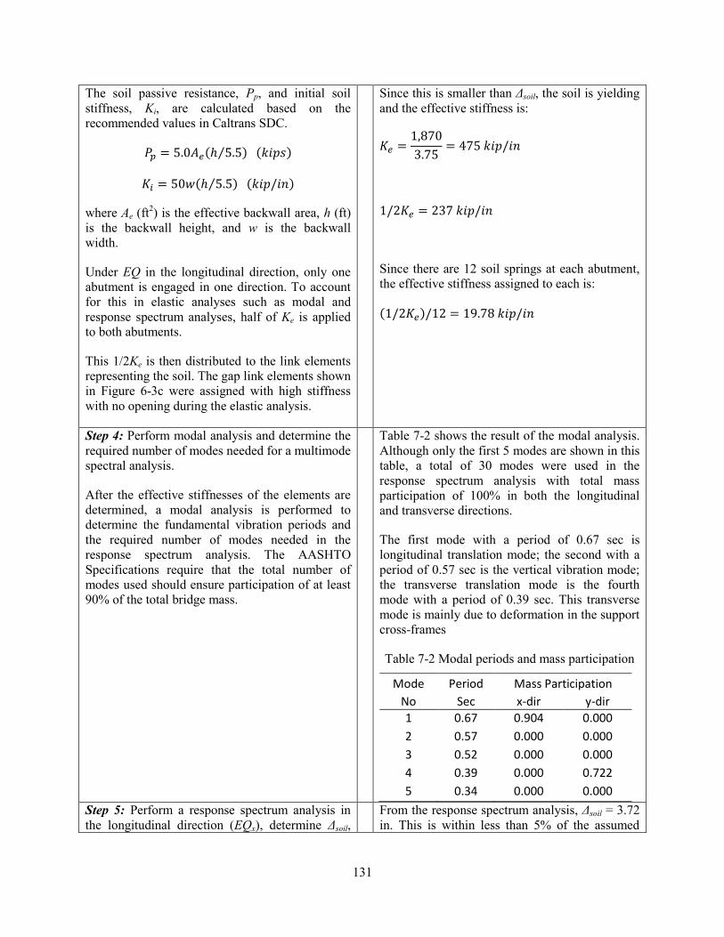
131
The soil passive resistance, Pp, and initial soil
stiffness, Ki, are calculated based on the
recommended values in Caltrans SDC.
( ⁄ ) ( )
( ⁄ ) ( )
where Ae (ft2) is the effective backwall area, h (ft)
is the backwall height, and w is the backwall
width.
Under EQ in the longitudinal direction, only one
abutment is engaged in one direction. To account
for this in elastic analyses such as modal and
response spectrum analyses, half of Ke is applied
to both abutments.
This 1/2Ke is then distributed to the link elements
representing the soil. The gap link elements shown
in Figure 6-3c were assigned with high stiffness
with no opening during the elastic analysis.
Since this is smaller than Δsoil, the soil is yielding
and the effective stiffness is:
Since there are 12 soil springs at each abutment,
the effective stiffness assigned to each is:
( )
Step 4: Perform modal analysis and determine the
required number of modes needed for a multimode
spectral analysis.
After the effective stiffnesses of the elements are
determined, a modal analysis is performed to
determine the fundamental vibration periods and
the required number of modes needed in the
response spectrum analysis. The AASHTO
Specifications require that the total number of
modes used should ensure participation of at least
90% of the total bridge mass.
Table 7-2 shows the result of the modal analysis.
Although only the first 5 modes are shown in this
table, a total of 30 modes were used in the
response spectrum analysis with total mass
participation of 100% in both the longitudinal
and transverse directions.
The first mode with a period of 0.67 sec is
longitudinal translation mode; the second with a
period of 0.57 sec is the vertical vibration mode;
the transverse translation mode is the fourth
mode with a period of 0.39 sec. This transverse
mode is mainly due to deformation in the support
cross-frames
Table 7-2 Modal periods and mass participation
Mode Period Mass Participation
No Sec x-dir y-dir
1 0.67 0.904 0.000
2 0.57 0.000 0.000
3 0.52 0.000 0.000
4 0.39 0.000 0.722
5 0.34 0.000 0.000
Step 5: Perform a response spectrum analysis in
the longitudinal direction (EQx), determine Δsoil,
From the response spectrum analysis, Δsoil = 3.72
in. This is within less than 5% of the assumed

132
and check against the initial value in Step 3.
The design spectrum is applied in the longitudinal
direction. Multimode spectral analysis is used and
the modal responses are combined using the
Complete Quadratic Combination (CQC).
value, thus, no further iteration is needed.
Step 6: Obtain the column forces due to EQx.
These forces will be combined with the forces due
to EQy to determine the design forces.
Table 7-3 Column forces due to EQx
Load P
(kip)
Mx
(k-ft)
My
(k-ft)
EQx 37 0 27,326
The seismic base shear of the bridge in the
longitudinal direction is 4,014 kips.
7.3.3 Design Loads
In the Type 2 design strategy, the design loads are from the DC, DW, and EQx only. A proposed R factor
of 1.5 is applied to EQx moments. The forces based on the Extreme Event I load combination are shown
in Table 7-4.
Table 7-4 Design loads for wall pier
Load/Combination P
(kip)
Mx
(k-ft)
My
(k-ft)
DC 1,991 0 0
DW 332 0 0
EQx 37 0 27,326
EQ1 = EQx/R 0 0 18,217
LC1: 1.25DC + 1.5DW + 1.0EQ1 3,024 0 18,217

133
7.4 Design of Wall Pier
Step 1: Determine the design axial load and
resultant moment from Section 7.3.3.
Table 7-5 Design axial load and resultant moment
Load
Comb.
P
(kip)
Mx
(kip-ft)
My
(kip-ft)
LC1 3,024 0 18,217
Step 2: Develop the axial force-moment (P-M)
interaction curve and check if the design loads are
inside the P-M curve.
The AASHTO ϕ factors are used in the interaction
curve.
The interaction curve about the weak axis (θ = 0o)
is developed.
From the final iteration the wall properties are:
w = 40 ft
t = 4 ft
ρv = 0.69% (#9 @ 6 in. = 158 - #8) vertical reinf.
ρh = 0.69% (#9 @ 6 in.) horizontal reinf.
f’c = 4 ksi
fy = 60 ksi
P = 3,024
My = 18,217 kip-ft (R = 1.5)
The interaction curve for θ = 0o is:
Therefore, the selected section and its
reinforcement are adequate.
0
10000
20000
30000
40000
50000
60000
0 10000 20000 30000 40000 50000
ϕP
n (
kip
)
ϕMn (kip-ft)
P-M curve @ 0 deg for EQx

134
Step 3: Determine the shear resistance in the
transverse direction.
Transverse direction is the strong direction of the
wall.
The factored shear resistance, Vr, of the wall pier
is taken as the lesser of (AASHTO Specifications
Art. 5.10.11.4.2):
√ and
* √ +
where ρh is the horizontal steel reinforcement
ratio.
ρh = 0.0069
b = 48 in.
d = 472 in.
√ ( )( )
[ √ ( )]( )( )
Therefore, Vr = 11,011 kips
Step 5: Check the vertical and horizontal
reinforcements.
The minimum vertical and horizontal
reinforcement ratio shall satisfy (AASHTO
Specifications Art. 5.10.11.4.2):
The spacing of vertical and horizontal
reinforcement shall satisfy (AASHTO
Specifications Art. 5.10.11.4.2):

135
7.5 Design of Support Ductile Cross-Frames
Step 1: Determine cross-frame force based on
nominal shear resistance of the pier.
The cross-frame shear force is equal to nominal
shear resistance of pier in the transverse direction.
where Vr is the factored shear resistance of wall
pier.
The corresponding cross-frame diagonal member
axial force with R factor applied is:
where N is the number of panels, θ is the angle of
the diagonal from the horizontal, and R is the
cross-frame response modification factor taken
equal to 4.0. In this equation, only one diagonal is
assumed resisting the shear force. This is because,
in a panel, one diagonal is in tension and the other
one is in compression. The compression diagonal
is expected to buckle in which case its post-
buckling resistance is considerably smaller, thus
the resistance is largely due to the yield resistance
of the diagonal in tension.
Vr = 11,011 kips
n = 5
θ = 22o
( )
Step 2: Determine the cross-frame force from the
response spectrum analysis in the transverse
direction.
Step 3: The design cross-frame force is the
smaller of PXF1 or PXF2.
In bridges with wall piers, it is expected that PXF2
would govern due to large shear resistance of
wall.
PXF = 152.43 kips
Step 4: Determine the cross-frame size.
The required area is:
A36 single angle
Fy = 36 ksi
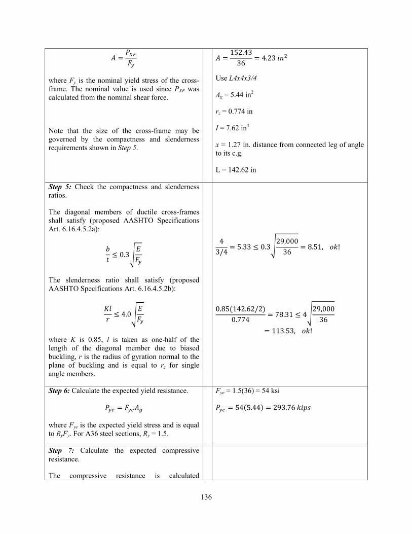
136
where Fy is the nominal yield stress of the cross-
frame. The nominal value is used since PXF was
calculated from the nominal shear force.
Note that the size of the cross-frame may be
governed by the compactness and slenderness
requirements shown in Step 5.
Use L4x4x3/4
Ag = 5.44 in2
rz = 0.774 in
I = 7.62 in4
x = 1.27 in. distance from connected leg of angle
to its c.g.
L = 142.62 in
Step 5: Check the compactness and slenderness
ratios.
The diagonal members of ductile cross-frames
shall satisfy (proposed AASHTO Specifications
Art. 6.16.4.5.2a):
√
The slenderness ratio shall satisfy (proposed
AASHTO Specifications Art. 6.16.4.5.2b):
√
where K is 0.85, l is taken as one-half of the
length of the diagonal member due to biased
buckling, r is the radius of gyration normal to the
plane of buckling and is equal to rz for single
angle members.
√
( )
√
Step 6: Calculate the expected yield resistance.
where Fye is the expected yield stress and is equal
to RyFy. For A36 steel sections, Ry = 1.5.
Fye = 1.5(36) = 54 ksi
( )
Step 7: Calculate the expected compressive
resistance.
The compressive resistance is calculated

137
according to AASHTO Specifications Art. 6.9.2.1,
6.9.4.1.1, and 6.9.4.1.2
(
)
The slender element reduction factor, Q, is equal
to 1.0 when:
√
o If Pe/Po > 0.44
[ ( ⁄ )]
o If Pe/Po < 0.44
( )
( ) ( )
√
( )( )
[ ( )]( )
Step 8: Calculate the maximum expected lateral
resistance of the cross-frames and compare against
the pier nominal shear resistance.
The maximum lateral resistance is the maximum
of:
( )
where Pt = 1.2Pye is the tensile resistance of the
diagonal member. The 1.5 factor is to account for
the upper bound of tensile resistance. The 0.3Pnc
term is taken to represent the post-buckling
resistance of the diagonal member. Vlat1 typically
governs particularly with relatively slender
diagonal members. Vlat2 may govern in cases
where the diagonal members are short and stocky.
The cross-frame maximum lateral resistance is
compared against the pier nominal shear
resistance to ensure elastic response.
( )
[ ( )]( )
[ ( )]( )
Therefore, Vlat = 2,295 kips
Step 9: Determine the superstructure drift and
check against limit.

138
After the cross-frame is designed, the
superstructure drift is determined. The
superstructure lateral displacement is calculated
using the equation:
where, PEQY is the force in the cross-frame
diagonal member determined from the response
spectrum analysis in the transverse direction and
Ae is the effective area calculated using Eqn.
(1-12).
The superstructure lateral drift should not exceed
4% (proposed AASHTO Specification Art.
6.16.4.5.1).
( )
( )
( )
( )
7.6 Cross-Frame Properties for Nonlinear Analysis
The expected force and displacement resistance of the cross-frames are calculated for use in the design
evaluation.
Step 1: Calculate the expected tensile yield
displacement.
The expected yield resistance is calculated in
Section 7.5 Step 6.
The effective axial stiffness is:
where E is the modulus of elasticity of steel which
is 29,000 ksi, Ae is the effective area calculated
using Eqn. (1-12), and L is the total length of the
diagonal member.
The expected yield displacement is then calculated
as:
L4x4x3/4
Pye = 293.76 kips
Ag = 5.44 in2
I = 7.62 in4
x = 1.27 in. distance from connected leg of angle
to its c.g.
( )
( )
( )
Step 2: Calculate the expected compressive

139
displacement.
The expected compressive resistance is calculated
in Section 7.5 Step 7.
The corresponding displacement is:
Pnc = 181.00 kips
7.7 Design Summary
The total weight of Ex. III-2 is 4,374 kips. From modal and response spectrum analyses, the periods,
forces, and displacements are:
Parameter Longitudinal Direction Transverse Direction
Fundamental period, T (sec) 0.67 0.39
Base shear, Vb (kip) 4,014 5,771
Pier displacement, Δpier (in) 3.57 0.15
Pier Base Shear, Fb (kip) 1,136 2,885
Deck displacement, Δdeck (in) 3.74 1.39
The wall pier properties are:
Width, w 40 ft
Thickness, t 4 ft
Vertical reinforcement #9 @ 6 in. (total 158 - #9) (ρv = 0.69%)
Horizontal reinforcement #9 @ 6 in. (ρh = 0.69%)
Factored shear resistance, Vr 11,011 kips
The cross-frame diagonal member section properties are:
Section L4x4x3/4 (A36)
Area, A 5.44 in2
Expected tensile yield resistance, Pye 294 kips
Expected compressive resistance, Pnc 181 kips
Maximum lateral resistance, Vlat 2,295 kips

140
7.8 Performance Assessment
The response under the the design earthquake and the MCE is discussed in this section.
7.8.1 Response under Design Earthquake
Figure 7-5 shows the pier force-displacement plots under the design earthquake. This is the shear force at
the base of the wall plotted against the displacement at top of the wall in the longitudinal and transverse
directions. The bridge response is dominated by the response in the longitudinal direction. The effective
yield shear resistance in this direction is equal to 857 kips and the corresponding yield displacement is
1.92 in. Although there is yielding the longitudinal direction, this yielding is only minimal. The average
displacement ductility in this direction was 1.7% and the maximum was 2.1%. In the transverse direction,
the wall piers are elastic: the shear force demand is much smaller than the shear resistance of the wall.
The inelasticity of the cross-frames even limited the shear force in this direction.
Figure 7-7 shows the total transverse shear force in the pier bearings plotted against the relative girder
displacement. Yielding in the cross-frames is apparent in these plots. The average girder drift was 2.3%.
7.8.2 Response under Maximum Considered Earthquake
Figure 7-6 shows the pier force-displacement plots under the MCE. In the longitudinal direction, there
was further increase of inelasticity in the wall pier. The average displacement ductility was 2.5% and the
maximum was 3.2%. The average displacement ductility in the longitudinal direction increases to 2.5%
indicating further increase of inelasticity. In the transverse direction, the force-displacement under the
MCE is about the same as that under the design earthquake due to yielding of the cross-frames.
Figure 7-8 shows further increase in the cross-frame inelasticity. The average girder drift under the MCE
was 3.7%.
This evaluation showed that the bridge behaved as designed. However, it can be observed that the wall
pier displacement ductilities in the longitudinal direction in this example are the same as those in Ex. III-
1. The bridge response is dominated by the longitudinal direction because the wall is significantly
stronger in the transverse direction.

141
Longitudinal Direction Transverse Direction
(a) DE1
(b) DE2
Figure 7-5 Wall pier force-displacement under the design earthquake
Longitudinal Direction Transverse Direction
(a) MCE1
(b) MCE2
Figure 7-6 Wall pier force-displacement under the MCE
-1000
-500
0
500
1000
1500
-6 -4 -2 0 2 4
Shea
r Fo
rce
(ki
p)
Displacement (in)
-3000
-2000
-1000
0
1000
2000
3000
-0.2 -0.1 0 0.1 0.2
Shea
r Fo
rce
(ki
p)
Displacement (in)
-800
-600
-400
-200
0
200
400
600
800
-3 -2 -1 0 1 2 3
Shea
r Fo
rce
(ki
p)
Displacement (in)
-3000
-2000
-1000
0
1000
2000
3000
-0.2 -0.1 0 0.1 0.2
Shea
r Fo
rce
(ki
p)
Displacement (in)
-2500
-2000
-1500
-1000
-500
0
500
1000
1500
2000
-10 -5 0 5 10
Shea
r Fo
rce
(ki
p)
Displacement (in)
-3000
-2000
-1000
0
1000
2000
3000
4000
-0.2 -0.1 0 0.1 0.2
Shea
r Fo
rce
(ki
p)
Displacement (in)
-1200
-1000
-800
-600
-400
-200
0
200
400
600
800
1000
-4 -2 0 2 4
Shea
r Fo
rce
(ki
p)
Displacement (in)
-3000
-2000
-1000
0
1000
2000
3000
-0.2 -0.1 0 0.1 0.2
Shea
r Fo
rce
(ki
p)
Displacement (in)

142
(a) DE1 (b) DE2
Figure 7-7 Superstructure transverse shear force – displacement under the design earthquake
(a) MCE1 (b) MCE2
Figure 7-8 Superstructure transverse shear force – displacement under the MCE
-2500
-2000
-1500
-1000
-500
0
500
1000
1500
2000
2500
-1 -0.5 0 0.5 1 1.5
She
ar F
orc
e (
kip
)
Displacement (in)
-2500
-2000
-1500
-1000
-500
0
500
1000
1500
2000
2500
-1.5 -1 -0.5 0 0.5 1
She
ar F
orc
e (
kip
)
Displacement (in)
-2500
-2000
-1500
-1000
-500
0
500
1000
1500
2000
2500
-2 -1.5 -1 -0.5 0 0.5 1
She
ar F
orc
e (
kip
)
Displacement (in)
-2500
-2000
-1500
-1000
-500
0
500
1000
1500
2000
2500
-3 -2 -1 0 1 2
She
ar F
orc
e (
kip
)
Displacement (in)

143
Chapter 8 Summary of Designs and Nonlinear Evaluation
8.1 Overview
The DSCF system is one of several techniques that can be used to protect columns from damage during
an earthquake. One advantage of this system over other forms of seismic protection is the smaller
superstructure and substructure displacements. However, the beneficial effect of the DSCF system is
diminished when: (a) the piers are designed to be flexible and (b) when the piers have a large ductility
demand (i.e. large R factor) in the longitudinal direction. The DSCF system works effectively when it is
more flexible than the piers. If the piers are more flexible, then they will yield before the cross-frames
undergo inelasticity. When the piers are designed to have a large ductility demand in the longitudinal
direction, the bridge response is dominated by the longitudinal response and the columns will yield even
though the DSCF system limits the transverse seismic forces transferred to the columns.
Experimental and analytical investigations showed that the DSCF system reduces the force and
displacement demand in the transverse direction of the substructure. The DSCF system is ineffective in
the longitudinal direction for a straight bridge due to its location and orientation. However, nonlinear
analyses of bridges designed using the Type 2 strategy showed that the bridge response in one direction
affects the total response. For example, the reduction of force in the column in the transverse direction
reduces the overall (resultant) force in the column. This overall response is important particularly when
bridge serviceability (i.e. minimal damage to the substructure) is required after an earthquake.
The nonlinear analyses showed that the proposed design procedure for the Type 2 strategy is adequate
since the bridges that were examined responded as intended. There was minimal yielding in the columns
such that they could be considered as essentially elastic even at the MCE level.
8.2 Design Summary
The example bridges designed using the Type 1 and 2 strategies are summarized in Table 8-1; the bridge
responses under the elastic multimodal spectral analyses are summarized in Table 8-2; and the plastic
shear capacities of the pier columns/wall are shown in Table 8-3.
As shown, the Type 2 design strategy resulted in a larger column size and more reinforcement. The
plastic shear capacities of the piers in the Type 2 design were more than 3 times the capacities of the piers
in the Type 1 design. However, the displacement demands in the Type 2 designs were less. In the bridges
with single-column piers, the transverse displacements were reduced by one-half when the Type 2
strategy was used. These comparisons may not be totally fair however because the two strategies are
based on different performance criteria. Damage in the substructure is expected when the Type 1 strategy
is utilized, while in the Type 2 strategy, bridge serviceability (i.e. minimal damage to the substructure) is
achieved even at the MCE level.

144
The interior-support cross-frames designed using the Type 1 strategy were significantly larger: the
diagonal member areas were about 3 to 4 times larger than those designed using the Type 2 strategy. No
special detailing is required for cross-frames designed using the Type 1 strategy; thus, the cross-frame
size is typically governed by the slenderness requirements. In the Type 2 strategy, the diagonal members
are detailed to promote biased buckling by welding the members at the point where they cross. Thus,
buckling of the diagonal member occurs only at half-length (length between the end of the diagonal
member and point where the diagonals cross) resulting in a smaller slenderness ratio. Due to the large
capacity and size of the cross-frames in the Type 1 strategy, the gusset plate connections may become
complicated.
Table 8-1 Summary of example designs
Pier Type Example
No.
Design
Strategy Pier Size
Reinforcement Support
Cross-Frames Long. Trans.
Single-
column
I-1 Type 1 4 ft diameter 1% 1% L8x8x5/8
I-2 Type 2 5.5 ft diameter 2.1% 1% L3x3x3/8
Two-
column
II-1 Type 1 4 ft diameter 1% 1.4% L8x8x5/8
II-2 Type 2 5.5 ft diameter 2.8% 2.6% L4x4x1/2
Wall III-1 Type 1 40 ft wide, 4 ft thick 0.69% 0.69% L8x8x1
III-2 Type 2 40 ft wide, 4 ft thick 0.69% 0.69% L4x4x3/4
Table 8-2 Summary of elastic seismic analyses results for the example bridges
Example
No.
Fundamental Period
(sec)
Bridge Base Shear
(kip)
Bridge Displacement
(in)
Longitudinal Transverse Longitudinal Transverse Longitudinal Transverse
I-1 0.92 2.23 1,285 524 4.92 11.58
I-2 0.64 1.27 1,943 975 3.49 5.78
II-1 0.98 0.68 2,676 3,731 5.06 3.37
II-2 0.61 0.48 4,350 5,569 3.34 2.25
III-1 0.67 0.30 4,014 5,095 3.74 0.58
III-2 0.67 0.39 4,014 5,771 3.74 1.39

145
Table 8-3 Summary of plastic shear capacities of the columns/wall
Example
No.
Plastic Shear Capacity
(kip)
Longitudinal Transverse
I-1 158 158
I-2 523 523
II-1 346 868
II-2 1,288 3,262
III-1 1,052 10,339
III-2 1,052 10,339
8.3 Summary of Nonlinear Design Evaluation
The performance of the substructures designed using the two strategies is assessed through displacement
ductility. This parameter is the ratio of maximum displacement to the yield displacement. It is deemed as
the best indicator of the magnitude of inelasticity or damage in the columns.
Figure 8-1 shows the comparison of the displacement ductility of the columns in the bridges with single-
column piers. The benefit of the Type 2 design is most apparent in the transverse direction where the
displacement ductilities are less than 1.0 even at the MCE level indicating that the columns were elastic.
In the longitudinal direction, the Type 2 design resulted in a smaller ductility, but the reduction was not as
large as that in the transverse direction. Nevertheless, the columns designed using the Type 2 strategy
were elastic.
Figure 8-2 shows the comparison of the displacement ductility of the columns in the bridges with two-
column piers. In these bridges, the difference in the ductility in the transverse direction is more
pronounced indicating the increased effectiveness of the ductile cross-frames. The ductilities in the
columns designed using the Type 2 strategy were all below 1.0.
Figure 8-3 shows the comparison of displacement ductility of the walls in the bridges with wall piers. The
ductility shown is for the longitudinal direction only because the wall behaves like a column in this
direction. The displacements in the transverse direction were exceedingly small. The ductility ratios were
the same for both bridges because the wall section is the same. This is because the R factors used in the
two designs were about the same: 2.0 for the Type 1 strategy and 1.5 for the Type 2 strategy. The
difference between the two strategies is in the wall transverse shear forces. The maximum transverse
shear forces in Ex. III-1 were 3,147 kips and 4,214 kips under the design earthquake and the MCE,
respectively. The maximum transverse shear forces in Ex. III-2 were 2,621 kips and 2,763 kips under the

146
design earthquake and MCE, respectively. The inelasticity and smaller cross-frames in Ex. III-2 resulted
in smaller transverse shear forces in the wall. Although inelasticity was also observed in the cross-frames
in Ex. III-1, the cross-frames in Ex. III-1 were larger resulting in larger transverse shear forces. As
discussed in Section 6.8, the cross-frames in Ex. III-1 experienced inelastic activity even though they
were designed using the Type 1 strategy. This was due to the large shear resistance of the wall pier in the
transverse direction causing the support cross-frames to undergo inelasticity before the yield shear
resistance of the piers was reached. This finding should serve as a cautionary alert when utilizing the
Type 1 design strategy for bridges with a stiff substructure. Inelastic response may occur in the
superstructure, which also suggests that failure may occur in the bearings and support cross-frame
connections.
These nonlinear evaluations showed that elastic columns can be achieved using the Type 2 design
strategy even at the MCE level. Therefore, this is one of several strategies that can be used to ensure
bridge serviceability after an earthquake. It was also shown that the pier support cross-frames will become
inelastic, even those designed according to the Type 1 strategy, as the pier transverse stiffness increases.
This suggests that, in bridges with non-integral wall piers, the pier support cross-frames should be
designed and detailed to undergo inelasticity even when the Type 1 strategy is used in the design.
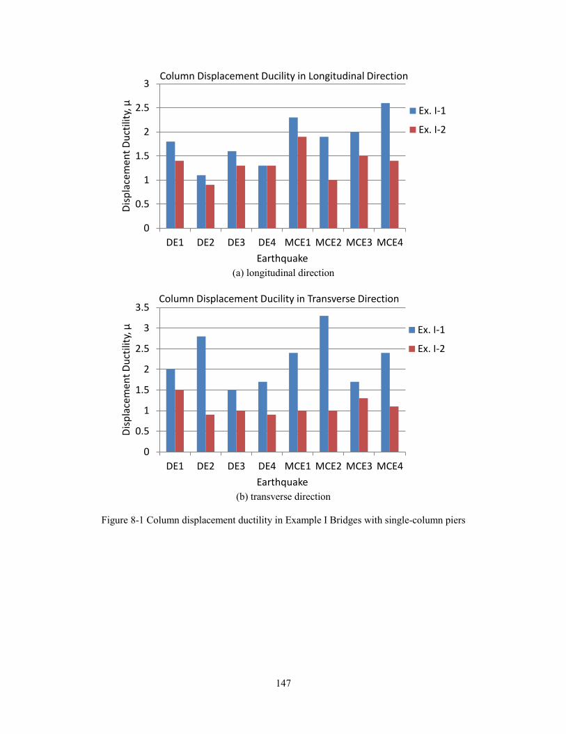
147
(a) longitudinal direction
(b) transverse direction
Figure 8-1 Column displacement ductility in Example I Bridges with single-column piers
0
0.5
1
1.5
2
2.5
3
DE1 DE2 DE3 DE4 MCE1 MCE2 MCE3 MCE4
Dis
pla
cem
en
t D
uct
ility
, μ
Earthquake
Column Displacement Ducility in Longitudinal Direction
Ex. I-1
Ex. I-2
0
0.5
1
1.5
2
2.5
3
3.5
DE1 DE2 DE3 DE4 MCE1 MCE2 MCE3 MCE4
Dis
pla
cem
en
t D
uct
ility
, μ
Earthquake
Column Displacement Ducility in Transverse Direction
Ex. I-1
Ex. I-2

148
(a) longitudinal direction
(b) transverse direction
Figure 8-2 Column displacement ductility in Example II Bridges with two-column piers
0
0.5
1
1.5
2
2.5
DE1 DE2 DE3 DE4 MCE1 MCE2 MCE3 MCE4
Dis
pla
cem
en
t D
uct
ility
, μ
Earthquake
Column Displacement Ducility in Longitudinal Direction
Ex. II-1
Ex. II-2
0
1
2
3
4
5
6
DE1 DE2 DE3 DE4 MCE1 MCE2 MCE3 MCE4
Dis
pla
cem
en
t D
uct
ility
, μ
Earthquake
Column Displacement Ducility in Transverse Direction
Ex. II-1
Ex. II-2

149
Figure 8-3 Displacement ductility in Example III Bridges with wall piers
0
0.5
1
1.5
2
2.5
3
3.5
DE1 DE2 MCE1 MCE2
Dis
pla
cem
en
t D
uct
ility
, μ
Earthquake
Column Displacement Ducility in Longitudinal Direction
Ex. III-1
Ex. III-2

150
References
AASHTO. 2012. AASHTO LRFD Bridge Design Specifications, American Association of State Highway
and Transportation Officials, Washington, D.C.
AASHTO. 2011. AASHTO Guide Specifications for LRFD Bridge Seismic Design, American Association
of State Highway and Transportation Officials, Washington, D.C.
AISC. 2010a. Specifications for Structural Steel Buildings, American Institute of Steel Construction,
Chicago, IL.
AISC. 2010b. Seismic Provisions for Structural Steel Buildings, American Institute of Steel Construction,
Chicago, IL.
Alfawakhiri, F. and Bruneau, M. 2001. ―Local versus Global Ductility Demands in Simple Bridges,‖
Journal of Structural Engineering, 127(5), 554-560.
Astaneh-Asl, A., Goel, S.C. and Hanson, R.D., 1985, Cyclic Out-of-Plane Buckling of Double Angle
Bracing. Report UCB/CE-STEEL-94/01. Department of Civil Engineering, University of California at
Berkeley, Berkeley, CA.
Bahrami, H., Itani, A.M., and Buckle, I.G. 2010. Guidelines for the Seismic Design of Ductile End Cross-
Frames in Steel Girder Bridge Superstructures, CCEER Report No. 09-04, Center for Civil Engineering
Research, University of Nevada, Reno, NV.
Carden, L.P., Itani, A.M., and Buckle, I.G. 2005a. Seismic Load Path in Steel Girder Bridge
Superstructures, CCEER Report No. 05-03, Center for Civil Engineering Research, University of
Nevada, Reno, NV.
Carden, L.P., Itani, A.M., and Buckle, I.G. 2005b. Seismic Performance of Steel Girder Bridge
Superstructures with Ductile End Cross-Frames and Seismic Isolation, CCEER Report No. 05-04, Center
for Civil Engineering Research, University of Nevada, Reno, NV.
Carden, L.P., Garcia-Alvarez, F., Itani, A.M., and Buckle, I.G. 2006. ―Cyclic Behavior of Single Angles
for Ductile End Cross-Frames,‖ AISC Engineering Journal, 2nd
Quarter, 2006, 111-125.
CSI. 2012. SAP2000, Computers and Structures, Inc., Berkeley, CA>
Goel, S.C. and El-Tayem, A. 1986. ―Cyclic Load Behavior of Angle X-Bracing,‖ Journal of Structural
Engineering, 112(11), 2528-2539.
Itani, A.M. and Goel, S.C. 1991. Earthquake Resistant Design of Open Web Framing Systems, Research
Report No. UMCE 91-21, Department of Civil and Environmental Engineering, University of Michigan,
Ann Arbor, MI.

151
Itani, A.M., Bruneau, M., Carden, L., and Buckle, I.G. 2004. ―Seismic Behavior Steel Girder Bridge
Superstructures,‖ Journal of Bridge Engineering, 1(8), 243-249.
Monzon, E.V., Itani, A.M., and Buckle, I.G. 2013a. Seismic Modeling and Analysis of Curved Steel Plate
Girder Bridges, CCEER Report No. 13-05, Center for Civil Engineering Research, University of Nevada,
Reno, NV.
Monzon, E.V., Itani, A.M., and Buckle, I.G. 2013b. Seismic Performance of Curved Steel Plate Girder
Bridges with Seismic Isolation, CCEER Report No. 13-06, Center for Civil Engineering Research,
University of Nevada, Reno, NV.
PEER. 2013. PEER Ground Motion Database, Pacific Earthquake Engineering Research Center,
Berkeley, CA.