NOTICE: When government or other drawings, speci- fications or other data are vised for any purpose other than in connection with a definitely related government procurement operation, the U. S. Government thereby incurs no responsihility, nor any obligation -whatsoever; and the fact that the Govern- ment may have formulated, furnished, or in any way supplied the said drawings, specifications, or other data is not to be regarded by implication or other- wise as in any manner licensing the holder or any other person or corporation, or conveying any rights or permission to manufacture, use or sell any patented invention that may in any way be related thereto.

»' -

REPORT NO. 1291262

00

^ ^AN INTRODUCTION TO MODULATION,

§ Q CODING, INFORMATION THEORY,

PROJECT TRIDENT

TECHNICAL REPORT

«=C GO C3 «cc

AND DETECTION

00

iß

ARTHUR D. LITTLE, INC. 35 ACORN PARK CAMBRIDGE, MASSACHUSETTS

DEPARTMENT OF THE NAVY BUREAU OF SHIPS NObsr-81564 S-7OO1-O307

DECEMBER 1962

DDC

TtölA o ■--' i

REPORT NO. 1291262

PROJECT TRIDENT

TECHNICAL REPORT

AN INTRODUCTION TO MODULATION,

CODING, INFORMATION THEORY,

AND DETECTION

by

Gordon Raisbeck

ARTHUR D. LITTLE, INC. 35 ACORN PARK CAMBRIDGE, MASSACHUSETTS

DEPARTMENT OF THE NAVY

BUREAU OF SHIPS NObsr-81564 S-7O01-O3O7

DECEMBER 1962

PREFACE

This is one of a series of technical reports

being issued by Arthur D. Little, Inc., under

Contract NObsr-81564 with the Bureau of Ships

as part of the Project TRIDENT.

attbur ZD.HittleJnr. S-7001-0307

FOREWORD

The object of this report is to explain some of the ideas in modern information theory and to show how they can be applied to certain problems in signal transmission and signal detection. It is not intended as a text or reference work. It evolved from several sets of lectures at various times and places to audiences of scientists and engineers who had no specialized knowledge of communications or information theory. The earliest sections, which introduce the fundamental ideas of amount of information and channel capacity, may nevertheless be of interest to readers with less technical back- ground .

We thank the Institute for Defense Analyses for permission to use herein portions of IDA Technical Note 60-19, "Modulation, Coding and In- formation Theory," which was written with the support of Contract NOSD-50 with the Advance Research Projects Agency; our colleagues J. Kaiser, G. Sutton, and others at IDA, who heard and criticized a series of lectures on which the Technical Note was based; our colleagues at Bell Telephone Laboratories, Inc., and Arthur D. Little, Inc., who likewise criticized sub- sequent oral presentations; Hugh Leney, M.S. Klein, and Paul B. Coggins of A. D. Little, Inc., and Professor John Wozencraft of M.I.T., who read and criticized the manuscript; and Claude E. Shannon, E. N. Gilbert, J. R. Pierce, C. C. Cutler, R. M. Fano and others from whose publications we have borrowed liberally.

iv

ABSTRACT

This is an expository essay on information theory for engineers interested in communications, sonar, and radar who have no specialized knowledge of statistical communica- tion theory. The fundamental concepts of information theory, and in particular, quantity of information and channel capacity, are defined and explained in simple terms. These concepts are used to make a quantitative estimate of the performance of several common modulation schemes and to analyze the performance of search and detection systems. The effectiveness of repeated or prolonged observations on detection thresholds and reliability of detection, and the relative performance of coherent and incoherent integration, are explained and illustrated quantitatively

artlnir ZB.HittlcJnr. S-7001-0307

TABLE OF CONTENTS

Page

List of Figures viii

List of Tables x

I. INTRODUCTION 1

II. GENERALIZED COMMUNICATION SYSTEM 2

III. DEFINITION OF INFORMATION 3

IV. APPLICATIONS TO DISCRETE CHANNELS 13

V. ENCODERS 15

VI. CHANNEL CAPACITY 22

A. CHANNEL CAPACITY OF AN ANALOG CHANNEL 22

B. CHANNEL CAPACITY OF SOME REPRESENTATIVE CHANNELS 30

C. COMPARISON OF VARIOUS PRACTICAL COMMUNICATION CHANNELS 32

VII. A NOTE ON PROBABILITY DISTRIBUTION 44

VIII. DETECTION AS A COMMUNICATION PROCESS 46

IX. COHERENT AND INCOHERENT INTEGRATION 56

X. CONCLUSION 72

BIBLIOGRAPHY 74

Vll

artbur ai.TUttlc.ilnc S-7001-0307

LIST OF FIGURES

Figure No. Page

1 A Generalized Communication System 4

2 An Idealized Information Source 4

3 Two Information Sources Combined into One 7

4 An Idealized Source with Outputs of Unequal Probability 7

5 Illustrating the Summing of Information from Two Independent Sources: H(x)=H(y>+H(z) 12

6 Illustrating the Summing of Information from Two Non- independent Sources: H(x)< H(y>+H(z) 12

7 Information in a 40-Letter Text Coded with a Simple Substitution Code 16

8 The Output of a Communication Channel Regarded as an Information Source 16

9 An Information Source 19

10 A Communication Channel 19

11 Sampling of a 3and-Limited Function of Bandwidth W 23

12 Multi-Dimensional Geometry 24

13 Transmitted and Received Signals in 2WT-Dimensional Signal-Space 26

14 Normalized Energy Per Bit Required to Signal Over a Noisy Channel 34

15 Spectrum of AM, Suppressed Carrier, SSB, and FM Waves when the Baseband Signal is a Single Cosinusoid 38

Vlll

LIST OF FIGURES (Continued)

Figure No. Page

16 Frequency-Modulation-With-Feedback (FMFB): Block Diagram of a Detector 41

17 Spectrum and Short-Time Spectral Density of an FM Wave 42

18 A Pulse for Constructing Band-Limited Function from Equally Spaced Samples 47

19 A Band-Limited Function Synthesized from Samples, Using the Pulse of Figure 18 47

20 Noise n(t) with and without a Low-Level Signal s(t) 49

21 Probability Distribution of Output of a Coherent Detector Whose Input is Waveforms like those in Figure 20 53

22 Random Noise n(t) with and without Superimposed Signal s(t) = S, Showing Samples 58

23 Samples, Squares of Samples, and Absolute Values of Samples in the Absence and in the Presence of Signals 59

^fk'Z ^ andL\i 24 / f, , 7 f, , and > f, in the Absence and in the Presence ■^ k i—- K ^—i I k|

of Signals, Compared with Expected Values 61

25 Distribution of Observations for Coherent, Square-Law, and Linear Rectifier Detection for Two Different Integration Times 62

IX

artbur ai.lUttle.ilnr. S-700i-0307

LIST OF TABLES

Table No. Page

I Probability of False Alarm Error and of Miss Error as a Function of Threshold Level and Signal-To-Noise Ratio 54

11 Expected Value and Variance of the Outputs of Several Types of Detectors 69

i s I

I. INTRODUCTION

Some paradoxes and misunderstandings about information have arisen in recent years as the science of information theory has been disseminated. The first misunderstanding is the belief that any intelligent person ought to know what the word information means.

In any specialized study, new concepts arise which have to have names Sometimes we name the concept after a person: Doppler shift, Plank's constant. Sometimes we give it a number or letter: The first law of thermodynamics. X-rays Sometimes we make up a new word: Meson, radio. But often we use a common word: Current, mass.

When a new technical concept is named with a common word, the word acquires a new meaning. It is impossible to use the word in a technical context im til that new meaning has been defined. Pressing a suit does not mean the same thing to a lawyer that it does to a tailor. And information does not mean the same thing to a communications engineer that it does to a police detective. There is no reason to expect anyone to know what the word information means to an information theorist unless he has been told.

In this report, we shall give the information theorist's definition of inform- ation, and some examples of how the word is used in its technical sense. In this way, we shall indicate why the concept is useful enough to be worth a name of its own, and attempt to show that the concept has enough in common with a nontechnical idea of information that no real violence is done to the language in appropriating this word to name it. Then we shall use the new concept as a tool to investigate the prop- erties of certain communication systems and detection systems.

It is possible simply to state a mathematical definition of information and proceed to demonstrate some of its properties. However, such an approach is like ly to be unconvincing, because the definition itself does not indicate just why it was chosen As an alternative, we shall discuss some reasonable and useful properties which we can hope a new definition of information will have, and use them to narrow down the search.

3rthur JH.lLittlcJnr. S-7001-0307

II. GENERALIZED COMMUNICATION SYSTEM

A generalized communication system is illustrated in Figure 1. The first element of this system is an information source. Although we have not yet defined what we mean by information, assume that the information source is a person talking. The output of the information source is called a message. If the information source is a person talking, the message is what he says.

The next element in the communication system is a transmitter ■ The transmitter transforms the message in some way and produces a signal suitable for transmission over the next element of this system, the communication channel. The input to the transmitter is the message, and the output of the transmitter is the signal. If the transmitter is a telephone handset, the signal is an electrical current proportional to the pressure of the sound waves impinging on the mouth- piece of the instrument.

The next element of this communication system is the channel. This is the medium used to transmit the signal from the transmitter to the receiver. While going through the channel, the signal may be altered by noise or distortion. In principle, noise and distortion may be differentiated on the basis that distortion is a fixed operation applied to the signal, while noise involves statistical and un- predictable perturbations. All or part of the effect of distortion can be corrected by applying the inverse operation or a partial inverse operation, but a perturbation due to noise cannot always be removed, because the signal does not always undergo the same change during transmission. In practice, the gamut of perturbation runs from noise to distortion. The input to the channel is the signal, sometimes called the transmitted signal. The output of the channel is the received signal, supposed to be in some sense a faithful representation of the transmitted signal.

The next element in this idealized communication system is the receiver. This operates on the received signal and attempts to reproduce from it the original message. It will ordinarily perform an operation which is approximately the in- verse of the operation performed by the transmitter. The two operations may dif- fer somewhat, however, because the receiver may also be required to combat the noise and distortion in the channel. The input to the receiver is the received signal, and the output of the receiver is the received message.

The last element of this communication system is the destination. This is the person or thing for whom the message is intended.

III. DEFINITION OF INFORMATION

An intuitively and esthetically desirable definition of amount of inform- ation will be a measure of time or cost of transmitting messages. When applied to a message source, the definition will give us a measure of the cost or time required to send the output of the message source to the destination. When applied to a channel, in the form information capacity of a channel, it will give a measure of how long it takes to transmit the message generated by one message source, or of how many message sources can be accommodated by one channel. We would like to be able to say that two comparable information sources generate twice as much information as one, and that two comparable transmission channels could transmit twice as much information as one.

The moment we identify information with the cost or the time which it takes to transmit a message from a message source to a destination, an interest- ing new fact emerges: Information is not so much a property of an individual mes- sage as it is a property of the whole experimental situation which produces the messages. For example, such utterances as: "How are you?, " "Glad to meet you, " "Happy Birthday, " "Congratulations on the birth of your child, " "Best Wishes to Mother on Mother's Day," carry very little information. These phrases belong to a very small set of polite stereotyped utterances, normally used in certain stereotyped circumstances. The telegraph company has taken advantage of this fact by listing on its telegraph blanks some 100 stereotyped messages for use in appropriate stereotyped situations. Tue customer chooses a message, and the signal transmitted by the telegraph company contains only the few symbols neces- sary to identify the particular message which has been chosen. At the receiving office, a clerk reconstitutes the stereotyped message for transmission to the des tination. The fact that such a stereotyped message contains less information than most utterances containing the same number of words is reflected in the lower cost to send such a message.

In order to get an effective definition of information, then, we shall con- sider not only the message generated or transmitted, but also the set of all mes sages of which the one chosen is a member. The message source may be con sidered as an experimental setup capable of producing many different outcomes at different times or under different stimuli, and the messages as the outcome of one particular experiment.

Consider an experiment X whose outcome is to be transmitted (see Figure 2). We will be particularly interested in cases in which the outcome of experiment X is an honest message, say written English or a television picture but for the moment consider experiments in general. First of all, suppose ex periment X has n equally likely outcomes. In this special case the definition of information evolves naturally from the following argument.

atthur JD.lUttlcJrtr. 3-7001-0307

TRANSMITTED MESSAGE

\

TRANSMITTED SIGNAL \

RECEIVED / SIGNAL

/

RECEIVED ^ MESSAGE

INFORMATION

SOURCE v TRANS-

MITTER /. CHANNEL 1 . RECEIVER /. DESTINATION

NOISE AND DISTORTION

FIGURE 1 A GENERALIZED COMMUNICATION SYSTEM

'EXPERIMENT X

INFORMATION

SOURCE

n EQUALLY LIKELY

OUTCOMES

FIGURE 2 AN IDEALIZED INFORMATION SOURCE

I

i The information in the message about X will be some function f(n).

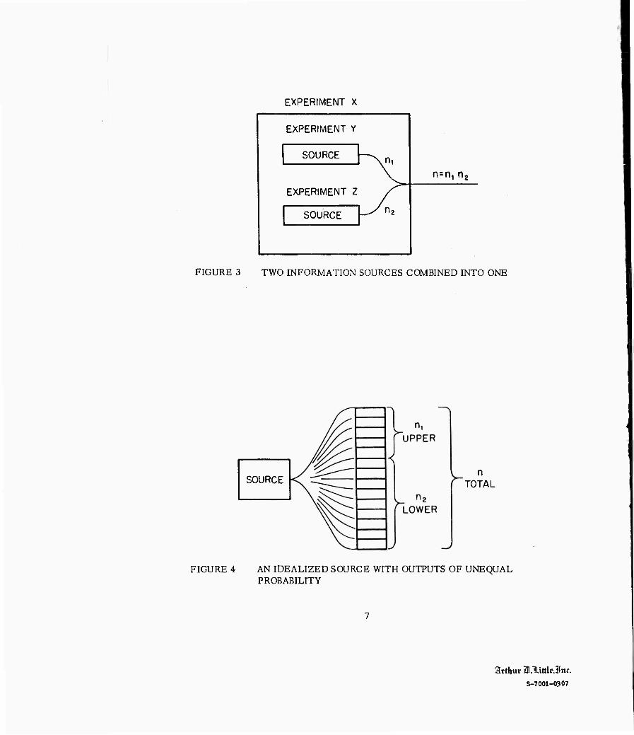
Suppose X is a compound experiment (see Figure 3) consisting of two independ- ent experiments , Y and Z, which have n^ and n2 equally likely outcomes. The total number of outcomes of the compound experiment is the product of nj and n2 , Transmitting the outcome of X is equivalent to transmitting the outcomes of Y and Z separately. Thus the information of X must be the sum of the informa- tions of Y and Z that is^

f(n)=f(n1) +f(n2)

where

n = n1n2.

This functional equation has many solutions. For example, f(n) might be the logarithm of nj or f(n) might be the number of factors into which n may be decomposed as a product of primes. However, there are other re- quirements of f(n). The time required to transmit the outcome of experiment X will certainly be an increasing function of n. Hence, we need consider only those solutions of the functional equation which are increasing functions of n. The only such solutions turn out to be constant multiples of log n, that is,

f (n) = c log n.

The simplest possible experiment we can imagine is one which has two equally likely outcomes, like flipping a coin. We use the information asso- ciated with such an experiment as the unit for measurement of information and call it one bit When this unit has been defined, the information in an experi- ment with n equally likely outcomes is then precisely log n bits.

Let us now test this definition of information and see if it does the things that we expect from it. For example, what is the information associated with an experiment whose outcome is certain? The experiment might be, for example to see whether the sun will rise between midnight and noon tomorrow. There is only one outcome possible:

n = 1.

The information associated with this experiment is

H = log2 1 = 0.

When the outcome of the experiment is a foregone conclusion, the information carried by the conclusion is zero.

attbur 31.luttlc.ilnr. S-7001-0307

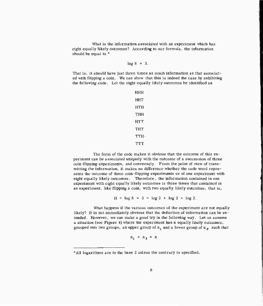
What is the information associated with an experiment which has eight equally likely outcomes? According to our formula, the information should be equal to *

log 8=3.

That is, it should have just three times as much information as that associat- ed with flipping a coin. We can show that this is indeed the case by exhibiting the following code. Let the eight equally likely outcomes be identified as

HHH

HHT

HTH

THH

HTT

THT

TTH-

TTT

The form of the code makes it obvious that the outcome of this ex- periment can be associated uniquely with the outcome of a succession of three coin-flipping experiments, and conversely. From the point of view of trans- mitting the information, it makes no difference whether the code word repre- sents the outcome of three coin-flipping experiments or of one experiment with eight equally likely outcomes. Therefore , the information contained in one experiment with eight equally likely outcomes is three times that contained in an experiment, like flipping a coin, with two equally likely outcomes, that is,

H = log 8 = 3 = log 2 + log 2 + log 2.

What happens if the various outcomes of the experiment are not equally likely? It is not immediately obvious that the definition of information can be ex- tended. However, we can make a good try in the following way. Let us assume a situation (see Figure 4) where the experiment has n equally likely outcomes, grouped into two groups, an upper group of nl and a lower group of n2, such that

nl + Hj = n

•"All logarithms are to the base 2 unless the contrary is specified.

EXPERIMENT X

EXPERIMENT Y

~"\ni SOURCE

EXPERIMENT Z

X\'X\y T\z

^y^z SOURCE

FIGURE 3 TWO INFORMATION SOURCES COMBINED INTO ONE

SOURCE n

TOTAL

FIGURE 4 AN IDEALIZED SOURCE WITH OUTPUTS OF UNEQUAL PROBABILITY

atthur ai.littlfjlnr. S-7001-0307

!

Let us assume that we are not really interested in the particular message gen- erated by the experiment, but only in whether the message is of the upper or of the lower group. We then have a situation where the significant output is one of two messages, having probabilities

for the upper message, and

Pi - ni + n2

P2 =

n2

i^ + n2

for the lower, respectively. One way to find out how much information is asso- ciated with this is to start with the information associated with the n equally probable outcomes, and subtract the excess information with the ^ or n, possible messages in the two sub-groups. The information associated with one message among n equally likely messages is

logn

The information associated with one message among nj^ equally likely messages is

log nj

This occurs not all the time, however, but only for a proportion of the time equal to n j/n. The information associated with one of nj equally likely messages is

logn2

and this occurs for a proportion of the time equal to ^/n.

Performing the arithmetic, we get

n n H = logn-—^— logni — log n2

= "Pi log P1 ■ P2 logp2.

I I I

Since Pj^ and p2 are less than unity, their logarithms are negative. Thus, one can see that the information H is positive.

This argument suggests a form for the amount of information in a message generated by experiment X having n possible outcomes which are not all equally likely. Let the various outcomes have probabilities pj, p 2, . . ., pn. In this case, the amount of information in the message generated by the experiment X is defined to be

H(x) = -p, log p - p log p - .. . -p log p *■*.£.£. n n

n

= ü "Pi iogPi 1=1

This sum bears a formal resemblance to a quantity called entropy in statistical mechanics. For tliis reason H(x) is also called the entropy function of p^ p2,

" " " Pn"

Let us now look at this definition to see if we think it is appropriate as a measure of information. First of all, when the n outcomes are equally likely,

1 Pi = n

log p. = logn

X -V0^i = 2 'n 1=1 i=l

= log n

logn

as it should.

It can be shown that for a fixed number of outcomes, the case of equally likely outcomes is the one in which H(x) attains its maximum value. This fits our intuitive notion very well: If all outcomes of the experiment are equally likely, the message gives a maximum of information; but if we have some a priori information that one outcome is more probable than another, then carrying out the experiment does not give quite so much information.

artbur ZD.HittlcJnc S-7001-0307

What if the experiment X consists of two independent experiments Y and Z? (See Figure 5.) Here the arithmetic is quite complicated, but ultim- ately one finds

H(x) = H(y) f H(z)

hi words, the information associated with X is the sum of information of its constituent experiments Y and Z. If Y and Z are not statistically independent* (see Figure 6), then

H(x) < H(y) + H(z)

This again is reasonable. Some of the H(y) bits of information about the Y ex- periment give information about the possible outcome of the Z experiment and so are counted twice in the sum H(y) + 11(2). So far, the definition of informa- tion which we have come up with seems satisfactory.

Let us recapitulate briefly. We started out with a model for a com- munication system which had an information source at one end and a destination at the other end. We have been looking for a definition of information which would be proportional to the time or the cost it takes to transmit the message from the message source to the destination. In order to get a firm hold on the problem, we successively restricted the information source until it was capable simply of putting forth n equally probable messages. In this case, we success- fully defined information as log n. We have generalized this definition slightly to the entropy function, which defines the amount of information generated by a message source capable of generating one of a finite set of n messages with known probability distribution. We have verified that this definition of informa- tion fulfills some elementary intuitive notions of how a measure of quantity of information ought to behave.

In a way, it does not seem that we have gone very far. The message source that we considered is extremely restricted, for it allows nothing more general than signals made up of discrete> uniquely distinguishable characters, such as teletypewriter messages. It does not include any message represented by a continuous wave form, such as the sound pressure of speech or the video signal which will generate a television picture. But surprisingly, the major

*Imagine the experiments Y and Z performed many times, and suppose that the results of the Y experiment are classified into sets according to the outcome of the Z experiment. Examine the probability distribution of the results of the Y experiment in each set: if the distribution does not vary from set to set, Y and Z are statistically independent. In plain but less precise language, the expected result of Y is the same whatever the result of Z.

10

I hurdle in defining quantity of information has already been passed. In spite of the fact that speech waves and television video signals are continuous signals, in any real life situation it is possible to distinguish only a finite number of tones or of picture intensities. The case of continuous messages can be re- duced to the case of discrete messages already discussed above, and the defini- tion of quantity of information can be directly adapted to this use.

11

arthur ai.\ittlc,3!nr. S-7001-0307

EXPERIMENT X

EXPERIMENT Y H(y)

INDEPENDENT

EXPERIMENT Z HU)

H(x)

FIGURE 5 ILLUSTRATING THE SUMMING OF INFORMATION FROM TWO INDEPENDENT SOURCES: H(x) = H(y)+ H(z)

EXPERIMENT X

EXPERIMENT Y H{y)

NOT INDEPENDENT

EXPERIMENT Z H(z)

H(x)

FIGURE 6 ILLUSTRATING THE SUMMING OF INFORMATION FROM TWO NONINDEPENDENT SOURCES: H(x) < H(y) + H(z)

12

1

IV. APPLICATIONS TO DISCRETE CHANNELS

Let us now look at some applications of the definition of information which has just been stated. Let us suppose that the experiment under considera- tion is that of shuffling a deck of 52 cards, and that the message is the particular order of the cards in the deck after shufQing. We shall define a perfect shuffle to mean that all of the possible orderings of the 52 cards are equally probable. Let us see how much information there is in a perfect shuffling experiment. The num- ber of possible arrangements of the cards, according to well known formulas in combinatorial analysis, is 52.' * The amount of information associated with this experiment is

log 52.' = 225.7 bits.

Now let us look at another kind of shuffling experiment: Cut the deck into two packs, top (T) and bottom (B), at a random place, and then interleave T and B together. The interleaving operation consists of 52 steps, at each of which the bottom card of either T or B falls onto the top of the shuffled deck. The shuf- fle is completely described by a sequence of 52 letters T or B. (The i-th letter is T if at the i-th step the card fell from the bottom of packet T.) The position of the cut may be found from the sequence by counting the number of T's. There are only 2 possible sequences of T and B, and hence only 252 possible outcomes of the shufflingexperiment. Even if we suppose all these outcomes to be equally probable, the maximum amount of information associated with this shuffling ex- periment is log of 252 , or 52 bits .

Suppose we now ask the question, how many times do you have to cut and interleave a deck in order to achieve something approximating a perfect shuffle? We learned earlier that the information associated with a sequence of independent experiments is not greater than the sum of the informations developed by the experiments independently. Each cut and interleave shuffling operation generates at most 52 bits of information. A perfect shuffle generates 225.7 bits of information. Therefore, no sequence of fewer than 5 cutting and interleaving shuffles could possibly generate a perfect shuffle. We can say with confidence that to shuffie a deck fairly by cutting and interleaving, you must repeat the operation at least five times. There is no guarantee, of course, that this will produce a perfect shuffling operation: All we have found out is that if you cut and interleave fewer than five times, it certainly will not produce a perfect shuffle.

»n'. = n(n-l)---3.2.1, e.g., 3'. = 3.2.1 = 6, 4'. = 4.3.2.1=24.

13

arthur ZD.lUttlcJnr. S-7001-0307

As another example, let us consider the information content of ordinary written English. To simplify the problems, let us Calk about "telegraph English, " which has no punctuation, no paragraphs, no lower case letters, and so forth. In this case, we have 27 symbols, the letters a to z and a space.

To get an upper limit to the amount of information, we can simply assume that all 27 symbols are equally probable. This sets an upper limit to the amount of information of log 27 = 4.76 bits per letter.

This estimate is certainly pessimistic, because we know that the letters are not equally probable. By carrying out a count of letters in a sufficiently large sample of text, we can get an idea of the relative probabilities of spaces and letters in English text. Using this data, we can apply the formula we have developed to find out that the information in English text is not more than about four bits per letter.

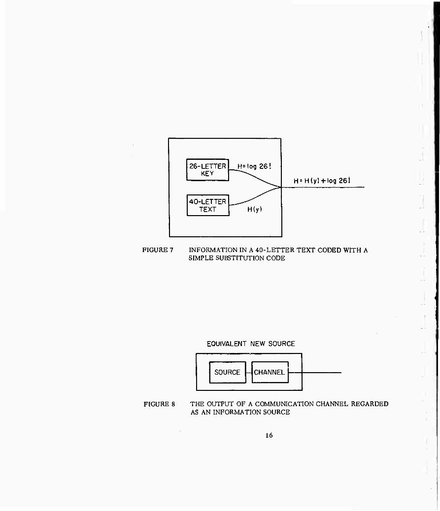
This estimate can be refined somewhat with observations taken from cryptography. Consider the construction of a substitution cryptogram. In such a cryptogram, for each letter in the alphabet some other letter is substituted. The table which tells which letter is substituted for which is called the key, and it is not hard to find that the number of possible keys is 26'.. If we view the cryptogram (see Figure 7) as a compound experiment X whose two parts are Y, the communi- cation of the clear text, and Z, the choice of a key from one of 26'. possibilities, the total information associated with this compound experiment is no greater than H(y) + log 26'. bits . We understand that substitution cryptograms of 40 letters can usually be solved, i.e., that given a 40-letter CJ yptogram, the information in both the text and the key can be recovered. Since 40 letters can contain no more than 40 log 27 bits of information, one concludes tliat

40 log 27 ^ H(y) + log 26'.

and hence that the information in a 40-letter English message is

H(y) «C 40 log 27 - log 26'. —100

The information in an English message is consequently no greater than 2.5 bits per letter.

By using more and more refined arguments, it has been shown* that the information content oi ordinary English text is about one bit per letter.

"See Reference 6 in the Bibliography.

14

V. ENCODERS

It is useful here to introduce the idea of an encoder. An encoder may be described as a purely deterministic device which converts a message in one set of symbols into a new message, usually in a different set of symbols. For example, a handwritten English message may be converted into a pattern of holes punched on a tape, then into a sequence of electrical impulses on a tele- type wire, back into English letters by a teletypewriter, and finally translated from English into French. The first three of these four operations are revers- ible encodings. That means that each incoming message can be encoded in only one way, and conversely, that no two different incoming messages are ever en- coded alike. Translation from English into French, however, is not usually an encoding, because it involves random choices. For example, the English word "robbery" may be translated into either "vol" or "brigandage." Even assuming that all such choices were settled in advance, one would undoubtedly find some French words representing several English ones, for example, "vol" for both "robbery" and "theft." Then the encoding would not be reversible.

A reversible encoder transforms messages into encoded messages in a one-to-one way; one gets the same amount of information from the encoded message as from the original message. One would like to conclude that a re- versible encoder driven by an information source is a new information source which generates information at the same rate as the driving source, However, this conclusion requires further assumptions about the encoder. For example, the encoder might just store the incoming message, and re-emit it at a slower rate. Such an encoder would ultimately require an unlimited amount of storage space. However, if a reversible encoder has only a finite number of internal states (for example, if it is made from a finite number of relays or magnetic cores or switching tubes with a finite memory), then the encoder output has the same information rate as its input.

We also need to talk about an idealized noiseless channel for trans- mission of discrete messages. An ideal channel has a finite list of symbols which it can transmit without error. A certain time is required to transmit each symbol. The times required to transmit the various symbols may not be the same.

The combination of a channel fed by a source may be regarded as a new source which generates the message at the receiving end (see Figure 8). The information rate of the received message will depend on the transmitting source. For example, suppose a channel can transmit English letters and word spaces at the rate of one symbol per second. When the channel transmits English text, it has a rate, as we have seen before, of about one bit per second. If the same channel is connected to a source which produces letters and spaces independently, with probability 1/27 for each kind of symbol, the rate is log 27 = 4.76 bits per second. The largest rate at which one can signal over a channel, for all choices of the source, is called the capacity of the channel. The capacity of the English letter channel just discussed is 4.76 bits per second,

arthur SLlMeJnr. S-7001-0307

H=log 261

H(y)

26-LETTER KEY

H=H(y) + log26!

40-LETTER TEXT

FIGURE 7 INFORMATION IN A 40-LETTER TEXT CODED WITH A SIMPLE SUBSTITUTION CODE

EQUIVALENT NEW SOURCE

SOURCE CHANNEL

FIGURE 8 THE OUTPUT OF A COMMUNICATION CHANNEL REGARDED AS AN INFORMATION SOURCE

16

I

In the example : of the English text source connected to the English letter channel, one feels that much of the capability of the channel is wasted. With an English text source as input, the channel transmits information at a rate much lower than that attainable with other sources.

Is it possible to speed up the source and still use the same channel? The answer is yes, and an encoder provides the means for doing so. It is possible to encode English text reversibly in such a way that the encoded mes- sages use fewer letters than the original messages. Then the encoded text may be transmitted at a higher information rate than the original text could.

In general, if we say that a channel has a capacity of C bits per second, we mean that the output of any source of information rate less than C bits per second may be transmitted over the channel by placing a suitable re- versible encoder between the source and the channel. No reversible encoder will transform the output of any source having an information rate greater than C so that it can be transmitted through the channel without error.

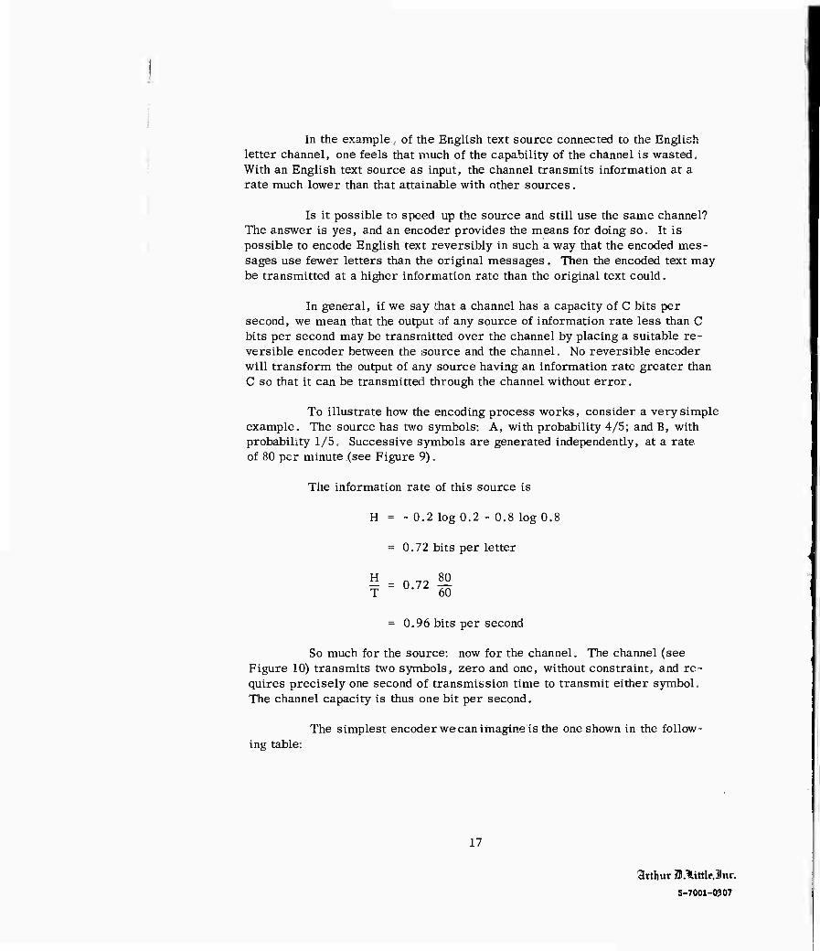
To illustrate how the encoding process works, consider a very simple example. The source has two symbols: A, with probability 4/5; and B, with probability 1/5. Successive symbols are generated independently, at a rate of 80 per minute (see Figure 9).

The information rate of this source is

H = - 0.2 log 0.2 - 0.8 log 0.8

= 0.72 bits per letter

M = 0.72 |° T 60

= 0.96 bits per second

So much for the source: now for the channel. The channel (see Figure 10) transmits two symbols, zero and one, without constraint, and re- quires precisely one second of transmission time to transmit either symbol. The channel capacity is thus one bit per second.

The simplest encoder we can imagine is the one shown in the follow- ing table:

17

Arthur ai.Htttlcilnr. S-7001-0307

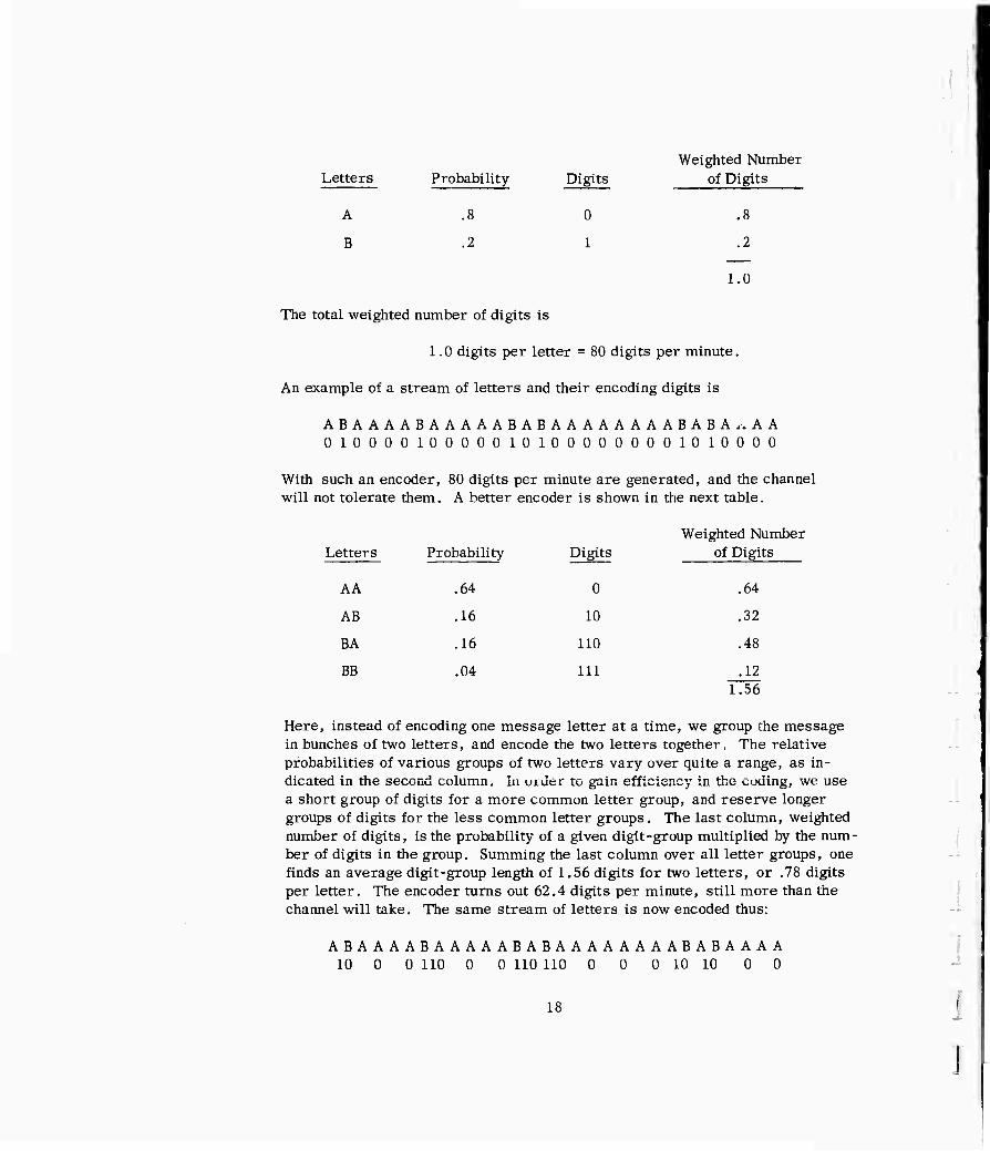
Weighted Number Letters Probability Digits of Digits

A .8 0 .8

B .2 1 .2

1.0

The total weighted number of digits is

1.0 digits per letter = 80 digits per minute.

An example of a stream of letters and their encoding digits is

ABAAAABAAAAABABAAAAAAAABABA^AA 010000100000101000000001010000

With such an encoder, 80 digits per minute are generated, and the channel will not tolerate them. A better encoder is shown in the next table.

Weighted Number Letters Probability

.64

Digits

0

of Digits

AA .64

AB .16 10 .32

BA .16 110 .48

BB .04 111 .12 1.56

Here, instead of encoding one message letter at a time, we group the message in bunches of two letters, and encode the two letters together. The relative probabilities of various groups of two letters vary over quite a range, as in- dicated in the second column. In uider to gain efficiency in the coding, we use a short group of digits for a more common letter group, and reserve longer groups of digits for the less common letter groups, The last column, weighted number of digits, is the probability of a given digit-group multiplied by the num- ber of digits in the group. Summing the last column over all letter groups, one finds an average digit-group length of 1.56 digits for two letters, or .78 digits per letter. The encoder turns out 62.4 digits per minute, still more than the channel will take. The same stream of letters is now encoded thus:

ABAAAABAAAAABABAAAAAAAABABAAAA 10 0 0 110 0 0 110 110 0 0 0 10 10 0 0

18

SOURCE OF 80 LETTERS PER MINUTE

A (prob. 0.8)

Blprob. 0.2)

FIGURE 9 AN INFORMATION SOURCE

CHANNEL TRANSMITS Oor 1

AT SIXTY SYMBOLS PER MINUTE

FIGURE 10 A COMMUNICATION CHANNEL (Will the Information from the Source

of Figure 9 pass through the Channel?)

19

atthur a.littlejnr. 8-7001-0307

■

The thirty letters are now encoded in 24 digits, 9 one's and 15 zero's. The reader can verify that if the digits are run together without spaces, they can still be separated unambiguously into symbols from our finite alphabet. Such a code is called segmented.

We can carry this a bit further, as shown in the next table.

Weighted Number Letters Probability

.512

Digits

0

of Digits

AAA .512

AAB .128 100 .384

ABA .128 101 .384

BAA .128 110 .384

ABB .032 11100 .160

BAB .032 11101 .160

BBA ,032 11110 .160

BBB .008 Hill .040

2.184

In this example, each group of three letters is encoded in a single digit-group. The more common letter groups are encoded in short digit-groups, and the less common groups in longer digit-groups. Doing the arithmetic exactly as before, we find that the average digit-group length for three letters is 2.184 digits. This results in an average of .728 digits per letter, and the coder produces 58.24 digits per minute, which can be transmitted by the channel. We already know that the information content of this source is .72 bits per letter, and therefore, no reversible encoder could encode it in less than .72 digits per letter on the average. The encoder illustrated is only about 1% less efficient than the ideal. The stream of letters given before is now encoded thus:

ABAAAABAAAAABABAAAAAAAABABAAAA 101 0 110 0 11101 0 0 100 101 0

The stream of 30 letters is now encoded in 22 digits, 11 one's and 11 zero's. The fact that the number of one's and zero's grow closer and closer together is not an accident. We know that the maximum capacity of a two-symbol source is reached only when the two symbols have equal probability. Our coder must bow to this fact if it is to use the channel efficiently.

20

This encoder must have some storage capacity, and must introduce some delay. For example, three incoming letters must arrive and be stored before the outgoing digit-group is identified. Furthermore, the long digit-groups are transmitted more slowly than the incoming three-letter groups are generated; and signals must be stored until a string of AAA's allows the encoder and trans- mission channel to catchup. In this simple example, no finite storage capacity will guarantee flawless performance, but the probability of exceeding a storage requirement of a few hundred symbols is extremely small.

The above example illustrates the general coding theorem, which can be loosely expressed as follows: Given a channel and a message source which generates information at a rate less than the channel capacity, it is possible to devise an encoder which will allow Lhe output of the message source, suitably encoded, to be transmitted through the channel.

21

arthur Ü.lAttlcJnr. 8-7001-0307

i

VI. CHANNEL CAPACITY

A. CHANNEL CAPACITY OF AN ANALOG CHANNEL

In the coding theorem stated in the previous section, we have implicitly defined the channel capacity of a channel: If a channel can transmit C binary dig- its per second (but no more), its channel capacity is C. It is easy to apply this definition to a channel which transmits strings of zero's and one's at a fixed rate, as in the example above. It is equally easy to apply it to a teletypewriter trans- mission channel which transmits sequences of letters and spaces at a rate fixed by the terminal equipment. But this is not really very useful, because there has never been very much doubt about the capacity of such a channel. Suppose we have a more general channel: How do we determine its channel capacity?

This question really hinges on a determination of how many distin- guishable signals the channel can transmit. To answer this question, we would like to have a way of identifying individual signals and distinguishing them one from another. What we really need is a catalog of signals.

Let us take as an example a channel capable of transmitting continuous waves with a finite bandwidth, free of distortion, but with uniform Gaussian noise of known power. Let us now identify and catalog the signals which can be trans- mitted through this channel.

We can get immediate help from the sampling theorem, a purely mathematical theorem now well known in the communication art, which will be stated here without proof (see Figure 11).

If a funtion of time f(t) contains no frequencies higher than W cycles per second, the function is uniquely determined by giving its ordinates a series of points spaced 1/(2W) seconds apart.

If we now let W be the bandwidth of the communication channel in question, we can identify any signal which the channel can transmit with a sequence of ordinates spaced 1/(2W) seconds apart. If we take a piece of this signal lasting only a finite time, say T, then the number of ordinates falling in this time range is 2TW.

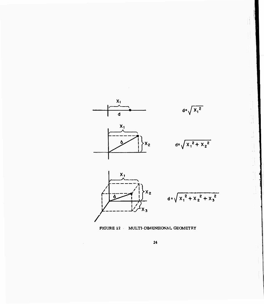
We can now introduce some geometrical ideas to help us along with the cataloging process (Figure 12). A quantity which is identified by one number can be represented as a point on the straight line. A quantity identified by two numbers can be represented by a point on a plane: This is the familiar procedure used to plot graphs A quantity identified by three numbers can be represented by a point in three-dimensional space. Similarly, our signal identified by 2TW

22

!

2WT SAMPLES

T

FIGURE 11 SAMPLING OF A BAND-LIMITED FUNCTION OF BANDWIDTH W

23

atthur JDAittlcJnr. S-7001-0307

Xi

«s/xi

•s/x7 2+x92

. A ^

7] I^X;

w ^ -PV^X

/x7+>^ + x7

FIGURE 12 MULTI-DIMENSIONAL GEOMETRY

24

numbers can be identified with a point in a (necessarily imaginary) geometrical space of 2TW dimensions. We imagine the 2TW identifying numbers to be the coordinates of a point, measured along 2TW mutually perpendicular axes.

If we compute energy E in the signal, we find, except for a scale factor, * that

p = 1 V 2 2W ZJ

Xn

where xn is the nth coordinate, i.e., the nth sample of f(t). If we compute the distance from the origin to a point in the space which represents the same signal, we find

d -Jl ^ Thus

d2 = 2WE

= 2WTP

wheic F is the bigaal power. Iii oilier WüIUS, in tills geometric visualization of continuous signals, geometrical distance is proportional to the square root of the power. The distance between two points in space is proportional to the square root of the power of the difference of the two signals which the points represent. Signals of power less than P all lie within the sphere of radius d = •Jl'WTP.

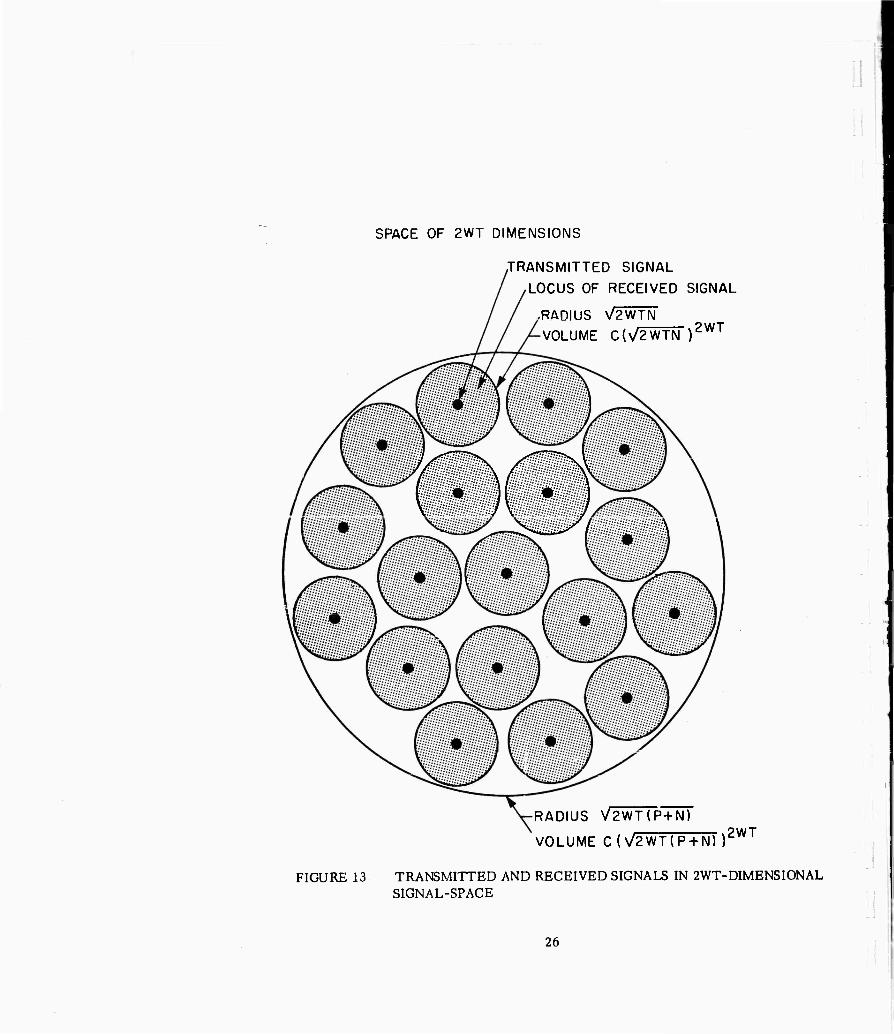
Now let us consider what happens to a signal as it goes through our channel. In Figure 13, we follow the geometric analogy, but represent the space of 2WT dimensions as two-dimensional space. A given input signal or output signal is represented by a point in the space. The distance between two points is proportional to the square root of the power of the difference of the two signals. Assume that the signal power is P, and that the power addedby the noise in the channel is N. Assume that we know the position of the point in space representing the signal before it is transmitted through the channel. Where is this point at the output end of the channel? We do not know exactly, but we know approximately. It is somewhere in a sphere of radiusN/2WTN centered around the point represent- ing the transmitted signal. In the figure, this sphere is represented by a hatched circle. Just as the area of a circle is proportional to the square of its radius, and the volume of the sphere is proportional to the cube of its radius, so the

''If the signal is electrical and f(t) is the instantaneous amplitude in volts, the scale factor is the real part of the circuit admittance in mhos. All sums are over the range (1, 2TW), unless otherwise stated.

25

artliur l.littlejnt. 8-7001-0307

SPACE OF 2WT DIMENSIONS

TRANSMITTED SIGNAL LOCUS OF RECEIVED SIGNAL

RADIUS V2WTN VOLUME C(\/2WTN ) 2WT

DQ

RADIUS V2WT(P+N)

VOLUME C(\/2WT(P + N) ) 2WT

FIGURE 13 TRANSMITTED AND RECEIVED SIGNALS IN 2WT-DIMENSIONAL SIGNAL-SPACE

26

volume of this hypersphere is proportional to the 2WT power of its radius, say,

' 2WT V = K( J2WTNJ

\ / where K is a constant whose numerical value is not important here.

The output of this channel consists of a signal plus noise, and has power approximately P + N. If we consider the whole family of possible outputs, they lie in a sphere of radius/s/2WT(P + N). In the figure, this is represented by the large circle. The volume of this hypersphere is

V = Kjsy^WT^-' w ' 2W1

where K is the same unspecified constant as before. Now let us assume that we have a number, M, of transmitted signals such that the regions of uncertainty associated with them when they are perturbed by the noise are nonoverlapping. Then the large hypersphere contains M nonoverlapping small hyperspheres. The volume of the large hypersphere is at least M times the volume of one of the small hyperspheres . If we write down this inequality and solve for M we get

/" "\ S \ II 12WT / / \2WT K(72WT(P+N)j ^MK 72WTN

2 WT //NTP\

ZVV1 TW

The ratio P/N is the familiar signal-to-noise ratio We can find the average rate of information transfer thus

logM<^ TWlog(l+P/N)

^ log M ^ W log (1 + P/N)

This gives us an upper limit for the channel capacity of this channel.

To get a more useful result, we need a lower limit also. In fact, the lower limit turns nut to be the same as the upper limit: We have an equality in- stead of an inequality. The details of the mathematical development are rather complex, and it is unnecessary to work them out here However, we shall sketch the idea behind the pre of, because it yields some important results.

27

artliur JJJUttlpJnr. 8-7001-0307

The idea is as follows. Oie fixes a certain number, M, of points in this space as signals, without regard for spacing to avoid overlapping regions, x^ particular selection of M points constitutes a particular code for transmitting signals. After having picked M particular points, one computes the probability of error at the receiving end. This"Is the probability that a point in the space (observed at the receiving end of the channel) which is close to one code point is also close enough to another point so that it might be wrongly identified. The probability of error is then averaged over all possible choices of codes. After going through all the arithmetic, geometry, and trigonometry, we obtain the following result:

i logM^Wlog(l+P/N) + ^logEav

where E is the averaged probability of error. (Note that E <^ 1, so that av o r- J av

log E is negative.)

We need to observe two things about this inequality. First, for some code choices, the error rate must be at least as low as the average error rate. Second, if we make T sufficiently large, we can make 1/T log E as small as desired, and hence we can make

— log M i

as close as we desire to

W log (1 + P/N)

and still make the average error rate as small as we please. Another way of saying this is

l.u.b. <i logMf = W logO ! P/N)

(where l.u.b. signifies least upper bound) for any value of average error rate, no matter how small.

We define this bound as the channel capacity, and can assert with confidence that there exist codes which permit transmission at a rate as close as desired to the channel capacity.

C = W log (1 + P/N)

with an arbitraily small error rate.

28

Some secondary conclusions can be drawn from this argument. First, the points which represent the signals in the code must be fairly well distributed throughout the space. This means that the wave form of these signals will look more or less like noise, not like anytliing with systematic structure.

Secondly, in order to achieve high signalling rates and low error rates, it is necessary to use a space with a large number of dimensions and a large number of distinct signals. For a model whose performance is reasonably typical of what can be done, Fano* finds error rate and signalling alphabet size to be related by

P(e)'^K 2 - va C/R

where

or

P(e) is the probablility of error

K is a constant of the order of unity

v is the number of binary digits constituting a message

2 is die nuiubei ui uistinct messages in the alphabet

C is the channel capacity

R is the actual signalling rate

and a is a particular function of R and C of the following form:

■R\ 1 R a = a ^ ^ i

AR C 4 ^ C ^

The model is a straightforward one in which the alphabet consists of two orthogonal signal wave-forms of equal energy, S, and equal duration, T; and in each time interval of length T, one and only one of the wave-forms is transmitted. For example, to achieve an error probability P(e) = 10 "5 with a signalling rate 95% of the capacity, i.e., R/C = ,95, requires v ~25, 000 bits per message .

*See Reference 4 in the Bibliography.

29

Stthur ai.1Uttlc.3lnf. S-7001-0307

There is a third effect which is troublesome: In such a coding system, the threshold effect gets very sharp. As long as the noise power density is no greater than that assumed, the error rate is small, but if the noise power exceeds a certain level, then a point is reached very suddenly where the error rate jumps to a large value.

Nevertheless, this formula is very useful, for it provides a standard of comparison against which transmission channels and transmission systems can be judged. As we shall see presently, it also suggests ways to increase the channel capacity of certain practical types of communication systems.

B. CHANNEL CAPACITY OF SOME REPRESENTATIVE CHANNELS

Let us now compute the channel capacity of some typical transmission channels. First, what is the channel capacity of a 100-word-per-minute tele- type (TTY) channel? This channel can transmit 600 letter or space characters per minute, or 10 characters per second. We saw before that the maximum in- formation associated with one such character is 4.76 bits, so that the capacity of this channel is 47 .6 bits per second - say 50 bits per second.

What is the channel capacity of an audio circuit for the transmission of speech? Being rother liberal, let us say that the signal-tn-nnise ratio P/N is 36 db, and that the bandwidth W is 4500 cycles per second. Such a channel is better than a telephone channel, and comparable to an AM broadcast radio channel. Working out the formula, we find that the channel capacity is 48, 000 bits per second - let us say 50, 000 bits per second.

What is the channel capacity of a channel used to transmit a video signal? Being rather liberal again, let us say that the signal-to-noise ratio P/N is 30 db, and that the bandwidth W is 5, 000, 000 cycles per second. Application of the formula in this case yields a channel capacity of 50, 000, 000 bits per second.

Thus, a ^oice circuit has about 1, 000 times the channel capacity of a teletypewriter channel, and a video circuit has about 1, 000 times the channel capacity of a voic:; circuit.

But is i: possible to send the output of 1,000 voice circuits through a single video channel, or to send the output of 1, 000 teletypewriter circuits through one voice channel? Not necessarily. As a matter of fact, many channels designed for video transmission will transmit very nearly 1, 000 voice circuits, but no one has ever squeezed 1, 000 teletypewriter channels into one voice channel of the kind just described and we do not expect that anyone ever will accomplish this feat.

30

'

We are usually satisfied to get 16 teletype channels into such a voice circuit, but sometimes use more elaborate equipment to get 48 circuits. By the use of ex- tremely elaborate terminal equipment, we appear to be able to get 100 or even 200 teletype channels into such a voice circuit.

There are three reasons for this limitation. First, an actual voice transmission channel usually is not an ideal channel in the sense we have described it, uniform, invariant with time, with no perturbation other than random noise. Most radio and telephone voice channels have distortion and nonrandom noise, such as interference and cross talk, but of a nature which does not interfere with human voice communication. These perturbations may disturb other kinds of signals, and hence effectively reduce the channel capacity. Second, when we deal with discrete signals, we normally have a very small signalling alphabet, and at the same time demand low error rates. For example, if we send in the form of pulses through an apparatus that detects the pulses one at a time, so that v = 1, about five pulses are required for each character; and if we require a character error rate of less than 10"4, then the error rate for an individual pulse must be P(e)^'2.10' . Solving the above equation for R/C gives R/QvO.OS; i.e., the number of teletype channels which could be multiplexed through one voice channel is about 0.03 x 1000 = 30. This value compares reasonably well with the observed value of 16, especially when we consider that the voice circuit for which the teletype multiplexer must be designed is usually a marginally satisfactory circuit having lower signal-to-noise ratio and smaller bandwith than the audio circuit described above. This consideration does not prevail in con- verting from television to voice and back, for the human listener does not decode the speech one bit at a time. He rather listens for whole phonemes, syllables, words, and even sentences before committing himself finally to a decision about what he has just heard.

Third, there is some loss, nevertheless, when a large channel is sub- divided, just as wood is wasted when a tree is sawed into planks . However, in a system (such as the Bell System L-3 cable carrier transmission system) which is designed to carry voice or television signals, the trade-off is at the rate of 600 to 800 voice channels per television channel, and most of the remaining discrep- ancy is accounted for by "Guard bands, " empty bands of frequency inserted be- tween adjacent channels to make channel separation easier at the terminals.

Let us recapitulate briefly. We have defined quantity of information, and the rate at which information is generated by a discrete source. We have computed the information generated by certain kinds of sources. We have de- fined the channel capacity of a discrete channel. We have defined the channel capacity of a band-limited channel with Gaussian white noise, and used the defini- tion to compute the channel capacity of certain kinds of channels. We have stated in loose form a theorem about encoding, to the effect that any channel can transmit the information from a source which generates information at a rate less than the channel capacity of the channel.

31

atthur ai.lUttlrJnr. S-7001-0307

C. COMPARISON OF VARIOUS PRACTICAL COMMUNICATION CHANNELS

Let us now go back to the formula expressing the channel capacity of a band-limited noisy channel, and do some manipulation with it. For example, how much energy must be supplied to transmit one bit of information?

Let

P = signal energy in watts per cycle-per-second

W = signal bandwidth in cycles-per-second

Then

PW = signal power in watts

Since

C = channel capacity in bits per second

then

PW C

Using the formula above for channel capacity C, one finds

—^ = energy in joules per ßit

PW = N ^/N_ C log ( 1 + P/N)

where

N = noise energy in watts per cycle-per-second.

In many practical situations, the noise energy per unit bandwidth is physically traceable to thermal effects, and is related to temperature by the formula

-23 N = KT = 1.37-10 T watts/cycle-per-second

where K is Boltzmann's constant and T is the absolute temperature. This rela- tion leads to the definition of an effective temperature or noise temperature

T = N/K e

even when the actual noise N may not be of thermal origin.

32

i The number of joules required to transmit one bit is directly propor-

tional to the noisiness or noise temperature of the channel, a relation which is quite understandable, and also to a certain function of the signal-to-noise ratio P/N. This function is plotted (Figure 14) as a function of the signal-to-noise ratio for easier analysis of its behavior. It is a steadily increasing function of P/N. Its minimum value is 0.693, which is approached when P/N is zero, that is, when the signal is very small compared to the noise. When the signal power density is as great as the noise power density, that is, when P/N equals one, the value of this function has risen from .693 to unity. Beyond that point it rises very rapidly. For the signal-to-noise ratios that we like to think of in communica- tions, 30 or 40 db, this function exceeds 100. The energy required to transmit one bit of information is 100 times greater when the signal-to-noise ratio is 30 db than when the signal-to-noise ratio is less than zero db.

This observation is not new, but it still comes as a shock to a great many people. Many will insist that it is not in accordance with experience, Why do we persist in using communication systems which use so much more energy than necessary to transmit information?

There are three principal technical reasons why most communication systems do not approach this ideal.

First, the modulation system does not make efficient use of bandwidth in reducing power required.

Second, the signal in its original form does not make efficient use of the channel provided, that is, the signal characteristics and the channel charac- teristics are not well matched.

Third, the information content of the signal is not commensurate with its characteristics. Most signals which it is desired to transmit contain a great deal of unnecessary detail, that is, they are greatly redundant. Redundancy may be useful, since it adds to the reliability, or accuracy of the message, but it is not usually present in a very efficient form.

All of these technical objections could be overcome or alleviated, at least in some degree, but the ultimate decision faced by the communications sys- tem engineer is based not on the desire to transmit a bit with the least possible amount of energy, but on the desire to satisfy a particular communication need at the minimum cost, hi most communication systems designed in the past, the cost of power has not been one of the principal system costs. However, when power does become an important part of the cost of the communication system, the designers will be driven to systems which operate with broader bandwidth and lower signal-to-noise ratio, in order to make the best possible use of power.

33

arthur HS.HittleJnc. S-7001-0307

100

10

P/N logd+P/N)

0.1

/

/

'— — .693

-10 10 20 (P/N) IN DECIBELS

30 40

FIGURE 14 NORMALIZED ENERGY PER BIT REQUIRED TO SIGNAL OVER A NOISY CHANNEL

34

In electronics systems involving the use of unattended equipment in satellites, power becomes an important factor because it must be generated by solar batteries or by some other relatively uneconomical means—uneconomical not only because of initial cost, but also because the power supply may take up a significant part of the total available space and weight. In passive communication satellite experiments such as Project ECHO, power is once again one of the limiting factors in performance . There is good reason to believe, therefore, that designers of communication equipment for use in active and in passive satellite communication relay systems will try to exploit the advantages of broad bandwidth, low signal-to-noise-ratio communication in the future.

In sending signals by radio, we can use various systems of modulation. These require various bandwidths and powers, and have various advantages depending upon the signal characteristics and system requirements. Let us see how close they approach the ideal of using only 0 693N joules to send a bit.

We will consider first three comparatively well-known modulation schemes: single sideband modulation (SSB), frequency modulation (FM), and frequency modulation with feedback (FMFB).

In single sideband modulation (SSB). a constant radio frequency is added to all frequencies in the baseband (voice, TV, or other) signal. For example, a baseband signal a cos 2 T ft might be represented as a modulation wave oCOs2ic(f0 + f)t, where fo is the carrier frequency. Figure 15 a and d illustrates the spectra of such signals. The rf bandwidth required is the same as the base- band bandwidth b The signal-to-noise ratio in the recovered baseband signal is the same as the rf signal-to noise ratio (assuming that no noise is added in amplification). That is,

S = P N _ N

where

S = baseband signal spectrum power density in watts per cycle- per-second (joules)

and P and N are defined as before. Thus

C = W log (1 + S/N)

= W log (1 + P/N)

35

atthuv aiJUölcJttr. 8-7001-0307

and

PW _ N P/N C log (1 + P/N)

P/N = (0.693N) 1.44

log (1 + P/N)

The system is less efficient than the ideal by a factor

P/N 1.44

log (1 + P/N)

For output signal-to-noise ratios required for good quality speech or television, this factor makes the system several hundred times less efficient than the ideal. The main advantage of SSB is its economy of bandwidth.

In amplitude modulation (AM), the baseband signal a cos 2 n ft is represented by the modulated signal (l+cos^nft) (cos 2n fot). By trigonometric identities this signal can be shown to be equal to

(a/2) cos 2 - (f - f) t+cos 2Tt f t+^/2) cos 2 TT:(f + f)t o o o

The AM spectrum is illustrated in Figure 15b. The constant carrier term, cos 2 K f0t can be removed by filtering to get a suppressed carrier AM signal, whose spectrum is illustrated in Figure 15c.

In AM, an rf band twice as big as the base bandwidth is required, be- cause two sidebands are transmitted. At full modulation, AM requires three times as much power, and with ordinary signal statistics, many times as much power, as SSB. However, when the carrier is suppressed, the system has the same power requirement as SSB, but still requires twice the bandwidth. The chief advantage of AM over SSB is the circuit simplicity.

In frequency modulation, the baseband signal n cos 2 rtft is represented by the modulated signal

cos (2 7if t + M cos 2"; ft) o

This cannot be expressed as a finite number of cosinusoids. How- ever, it can be expressed as

V J (M) cos 2 - (f + n f)t / . n i o

where J (M) is the Bessel function of order n and argument M.

36

i

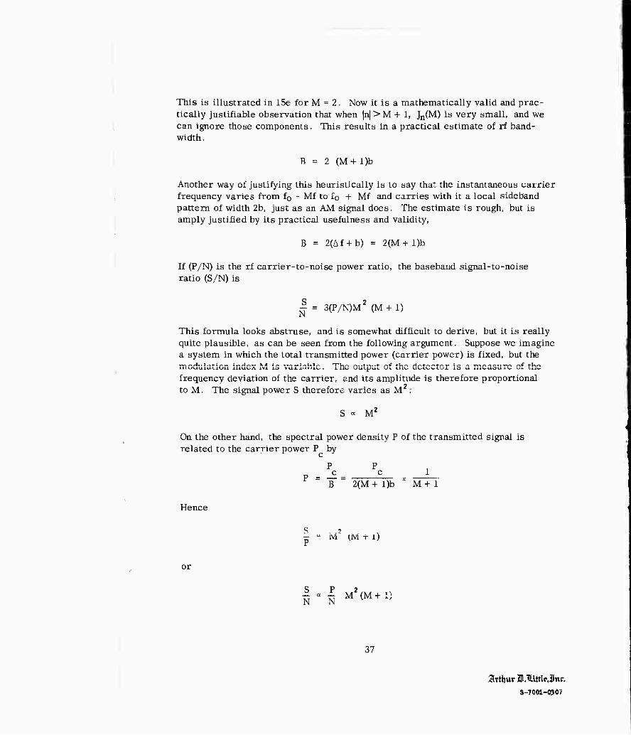
This is illustrated in 15e for M = 2. Now it is a mathematically valid and prac- tically justifiable observation that when |n|>M + 1, Jn(M) is very small, and we can ignore those components. This results in a practical estimate of rf band- width .

B = 2 (M+l)b

Another way of justifying this heuristically is to say that the instantaneous carrier frequency varies from fo - Mf to fo + Mf and carries with it a local sideband pattern of width 2b, just as an AM signal does. The estimate is rough, but is amply justified by its practical usefulness and validity,

B = 2(Af+ b) = 2(M+ l)b

If (P/N) is the rf carrier-to-noise power ratio, the baseband signal-to-noise ratio (S/N) is

| = 3(P/N)M2 (M+l)

This formula looks abstruse, and is somewhat difficult to derive, but it is really quite plausible, as can be seen from the following argument. Suppose we imagine a system in which the total transmitted power (carrier power) is fixed, but the iiiOOUi-«^L±Uli XilU^A iVl XO Vd..L-LU-lJiC- . illV^ wUL^Ui- ^Ji- LI 1^ UOL^WL^J. iO *A Ai.!^ lAO U-t. W <J± i-XiC

frequency deviation of the carrier, and its amplitude is therefore proportional to M. The signal power S therefore varies as M2 :

S - M2

On the other hand, the spectral power density P of the transmitted signal is related to the carrier power P by

Hence

P =

S

P

P P c c

B 2(M + l)b M + 1

M ^M + t)

or

S P 2 — « — M (M + 1)

37

Arthur ai.üittlcjnr. S-7001-03Ö7

BASEBAND SIGNAL

f

(o)

AMPLITUDE MODULATED

SIGNAL

^•BASEBAND b

fcH i

fo

|fo+f (b)

SUPPRESSED RF BAND 2b—-^

CARRIER AM v-. Ho+f (0

SINGLE RF BAND 2b—'

;

SIDEBAND |Vf (d)

FREQUENCY RF BAND b — JZ r~

MODULATION ■ (e) OF INDEX 2 . . 1 1 1 JL 1

RF BAND (approximate) 2b(2+1)

FIGURE 15 SPECTRUM OF AM, SUPPRESSED CARRIER, SSB, AND FM WAVES WHEN THE BASEBAND SIGNAL IS A SINGLE COSINUSOID

38

There only remains the evaluation of the constant of proportionality. A more detailed analysis shows that the correct value is three. The analysis is com- plicated by the fact that the demodulated noise spectrum density of an FM channel is not uniform, but is proportional to demodulated frequency.

For an FM detector system to work, it is necessary that the carrier amplitude be large in comparison with the noise amplitude. It is not hard to see why: the discriminator must be able to follow unambiguously the coherent pattern of peaks and dips in the sinusoidally oscillating signal. If the noise is too big, a loop of the sinusoid will be cancelled out from time to time, or an extra peak or dip added. Under these conditions, the discriminator will make an erroneous identification of phase and will skip or add an apparent full cycle. Practically speaking, this hazard is reduced to negligible proportions only if the carrier-to- noise ratio is at least

~ = 16, or 12 db N

As the index M is increased, the required rf bandwidth is increased; hence, the total rf noise is increased, and the minimum permissible transmitted power is increased. On the other hand, increasing the deviation makes the baseband signal-to-noise ratio greater than the carrier-to-noise ratio.

The channel capacity at minimum power level is

C = b log (1 + S/N)

= b log

Hence, the energy per bit is

2 71 1 +48MZ (1 +M) !

PB - (0.693N) 46(1+M)

C " ^•"7""' log [1+48M2(1 + M)]

The energy is greater than the ideal of 0.693N by a factor

46 (1 + M)

log i 1 + 48M2 (1 + M)|

This factor has an optimum value of about 15, consistent with an index, M, of two and an output, S/N, of 600 or 27 db. Thus, ordinary FM is at best about 15 times less efficient in the use of power than the ideal. The efficiency of FM is relatively

39

arthur ZD.IUttleJnc. S-7001-0?07

.1

insensitive to variation of index M from 1 to 4. The corresponding range of signal- to-noise ratios is 20 to 35 db. This range is of considerable practical interest for voice and many other analog signals.

Figure 16 shows a block diagram of frequency modulation with feedback, called also Chaffee system or FMFB.

In an FMFB system, we use the output of the discriminator to cause a beating oscillator partially to track changes in carrier frequency. Of course, it cannot track perfectly, for in that case the output of the mixer would have constant frequency and there would be no signal for the discriminator to detect. However, if a frequency change 5f at the detector causes a change |i6f in the voltage tuned oscillator, then the deviation M. in the intermediate frequency amplifier is reduced to

M. i 1 + ji

Here p. is completely analogous to the gain in the feedback loop of a linear ampli- fier, and the amount of feedback in db is

feedback = 20 log 0 g. db

Thus we can cut down the intermediate frequency bandwidth B. to a value

. 2 / M A , \i + u j

Inasmuch as the IF bandwidth is less than the total rf bandwidth, the noise in the IF band is less than that in the rf band. We will still need a 12-db carrier-to-noise ratio at the discriminator, but the rf carrier-to-noise ratio can be less by the ratio of the IF bandwidth to the rf bandwidth.

Another way of expressing this idea is illustrated in Figure 17. The spectrum of the FM wave, as described before, extends from f - 3 to f + 3..

o f o f This spectrum is illustrated in Figure 17a. However, over a short period of time an investigation of spectral energy density will show the energy to be concentrated about the instantaneous frequency in a band of breadth about 2b. This is depicted in Figure 17b. A filter of bandwidth 2b located at the right center-frequency would pass almost all the signal energy. The effect of the feedback loop in the detector is to shift the effective center frequency of the IF filter almost in synchronism with the instantaneous frequency of the incoming carrier.

40

FM INPUT BANDWIDTH S BANDWIDTH B, BANDWIDTH b-

MIXER l-F FILTER

AND AMPLIFIER

LIMITER

VOLTAGE TUNED

OSr.lLLATOR

FREQUENCY DETECTOR

FIGURE 16 FREQUENCY-MODULATION-WITH-FEEDBACK (FMFB): BLOCK DIAGRAM OF A DETECTOR

41

arthur ZB.lUttlcIlwf. S-7001-0307

AMPLITUDE

SPECTRUM OF AN FM WAVE

C0S(2Trf0t+ ZCOSZTTM) (0)

fo-3f | Ml0 I fo+3f

^ I ! I LJ L_i ^_

SHORT-TERM SPECTRAL DENSITY OF AN FM WAVE

TIME

FREQUENCY

(b)

INSTANTANEOUS FREQUENCY

2b

FREQUENCY

FIGURE 17 SPECTRUM AND SHORT-TIME SPECTRAL DENSITY OF AN FM WAVE

i

42

I

The minimum allowable signal-to-noise ratio now becomes

^ = 16 MB.

i

An analysis like the one performed above leads to a required energy-per-bit of

^ / M ,\

c ' n ..„>,»„. M log |"l+48M2(l+T^-)J

This energy is greater than the ideal by a factor

46(IT^+1)

log[l+48M2(l + Y^J]

This expression is only approximate, because when M is very large, the minimum allowable discriminator signal-to-noise ratio is greater than 12 db. When this is accounted for, this factor is found to go asymptotically to a theoretical value of two as M is increased. Experimentally, it appears that one can achieve a value around three, i.e., that one can operate with only three times the minimum theoretical power requirement given by information theory.

That is, it is possible to receive information with a receiver power of:

P = 3(0.693)CN

= 3(0.695)CKT watts

where T is the effective noise temperature, and K is Boltzmann's constant, e

Phase lock reception is similar to the foregoing system except that the local oscillator is in effect made to track the received signal in phase.

Some pulse transmission systems, such as pulse position modulation, appear to be capable of as great a power efficiency as FMFB. Whether or not they are competitive will depend upon equipment economy and, in some cases, upon the kind of information that is to be transmitted.

It should be noted that the channel capacities attributed to various modulation systems above are not binary digit signalling rates. We have accepted at face value the value which the channel capacity formula gives for the demodulated baseband channel, and compared that with the rf power. This comparison is still fair, however, if we are dealing exclusively with analog channels.

43

Arthur ai.lLtttlcJnr.

S-7001-0307

VII. A NOTE ON PROBABILITY DISTRIBUTION

In dealing with collections of numbers having properties of randomness, such as observations of electrical noise, it is convenient to introduce certain concepts from statistical analysis. In particular, let us assume we have a col- lection of numbers x , x , x x^,, and define the following:

N

m = the mean = — / , x N fe=j m

N 2 , 1 ^T1 2 2

s = the variance = — > x - m N /j m 1

m=l

The mean is what we call in plain language the average. The variance is more esoteric: the square root of the variance, s, is called the standard deviation, and is a measure of the extent to which the numbers x^,, scatter from the mean value m.

Under many circumstances the set of N numbers is taken from a much larger or infinite set, called the population. This set of N numbers is then called a sample. The population mean |i and population variance o2 are defined just as

the number of elements, N, in the sample is large, we are often justified in treating the sample mean m and variance s as about equal to the population mean n and variance 0 .

If each element xm of the population is the sum of a large number of statistically independent numbers then (with certain technical restrictions) the distribution of values of the elements Xjn will approach a particular distribution, called the Gaussian or normal distribution, characterized thus: in any random sample of N elements, the number of elements having a value between x and x + Ax is approximately

I— ~|

N Pi (x -l-O/o A x/o j o —i

where P(u) is the normal probability distribution function

1 - u2/2 P(u) = .= e

44

The normal probability dislribution has been extensively studied, and is a satisfactory model for a wide variety of statistical phenomena. Sums and dif- ferences of normally distributed independent numbers are also normally dis- tributed. For example, we can take sums of the elements x M at a time, thus

M 2M (k+l)M yo = E V yi = S V yk = E x

1 M+l kM+1

n

n

Then the population of all possible values of y^ has a mean M \j, and a variance Ma2- This and other properties of normal distributions will be referred to often in the next sections, and are described and proved in texts on probability.

45

aitbuT ai.lUttlcJnr. 8-7001-0307

Vm. DETECTION AS A COMMUNICATION PROCESS

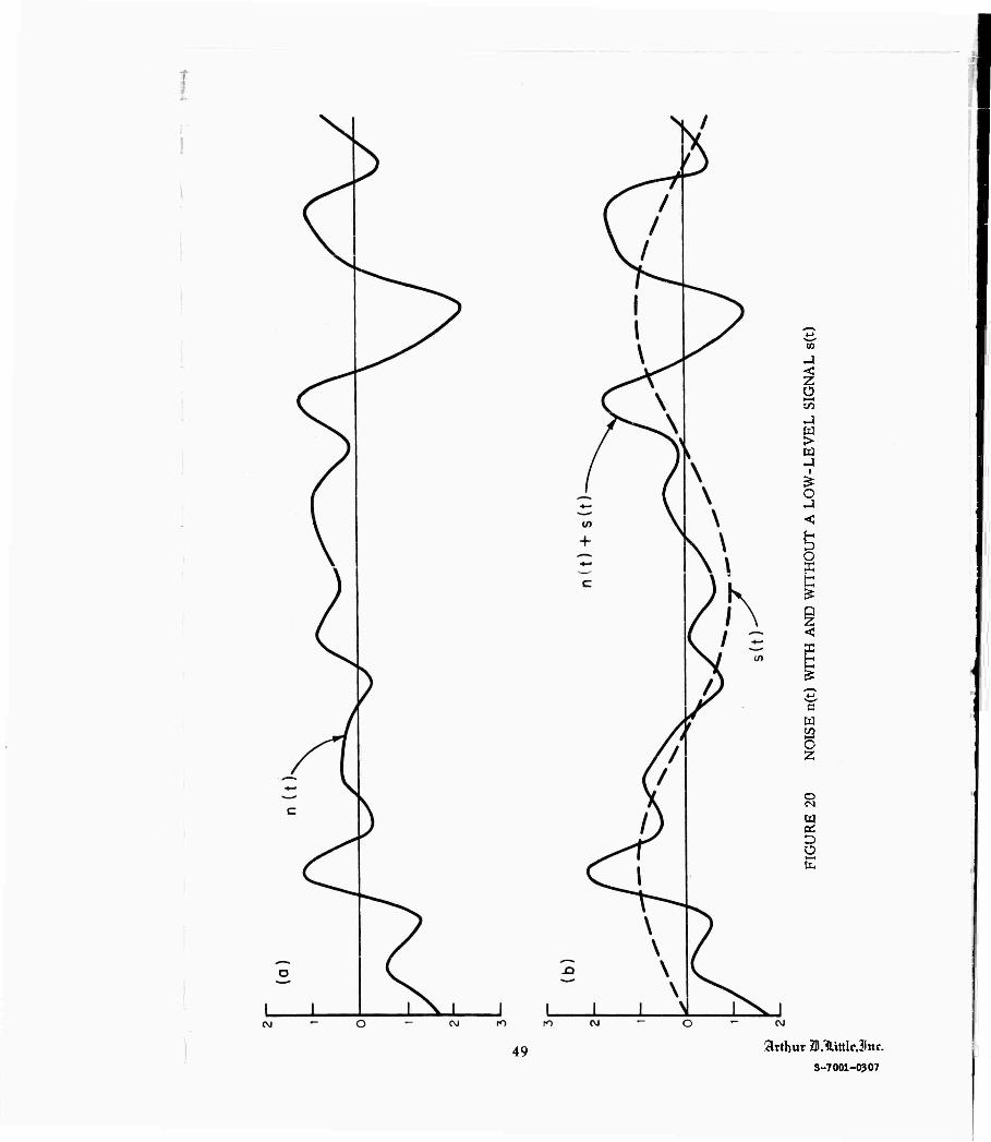
Detection of a signal such as a radar echo in a background of noise may be treated as a communication process also. Suppose, for example, a situation exists where a signal s(t) may or may not be present in a background of noise n(t). Let us suppose for illustration that the noise is Gaussian with a uniform power density spectrum N up to a maximum frequency W, that the signal falls in the same frequency range, and that our observation is limited to the period of time O^t ^T, which is supposed to include all of the nonzero part of the signal s(t).

Using the sampling theorem as before, we can represent the signal by a point in 2WT-dimensional space. It is convenient to make a slight scale-change and represent a function f(t) by*

2TW

where

k=l

,(t)= v/2W

k^k

sin 2TiW(t - k/2W) ^' = ^ "W 2rtW(t-k/2W)

f. = ^L f(k/2W)

Figures 18 and 19 show graphically how a function f(t) is built up of such ele- ments cp.

It is not hard to show that c

q, (t)(p„ (t) dt = 0 if k ? l 1 if k = -C

Given two functions f(t) and g(t), we can define a scalar product

2TW

f(t) ■ g(t) = 2 fkgk

"Unless otherwise indicated all sums are over the range (1, 2TW) and all integrals over the range (-cc, «;).

46

!

/ /

/"

/

/

\ \ \ \

SIN 2TrWT 2irwT

.-^*-

FIGURE 18 A PULSE FOR CONSTRUCTING BAND-LIMITED FUNCTION FROM EQUALLY SPACED SAMPLES

SIN 2TnwT-1)

FIGURE 19 A BAND-LIMITED FUNCTION SYNTHESIZED FROM SAMPLES, USING THE PULSE OF FIGURE 18

47

artbur i.mttlejttc. S-7001-0307

From the above integral relation it follows that

°? 2TW

'A

which provides an alternative formula for the scalar product. Following this notation we let

3(t) =2 sk<Pk, n(t) =y nv k k

We may call the total signal energy S, and we see that, in suitable units,

s2 (t) dt = S = V

The total noise energy is the product of noise spectral density, bandwidth, and time.

p(t)dt =7^ NWT = | n^t) dt = > n*

ihe expected value of r^. for any k is therefore N/2. To avoid a sticky prob- lem, we can assume the noise sample amplitudes n^ have expected value zero and variance N/2 and that they are independent and normally distributed. This is a satisfactory definition of white Gaussian noise of power density spectrum N and bandwidth W.

Now let us consider the detection problem where the noise field n(t) is present, and the signal s(t) may or may not be present. We observe a received signal f(t) where

f(t) = s(t) + n(t) =y (s + n ) <p when the signal is present.

= n(t) = ^V-1 n <p when the signal is absent.

Figure 20, a and b, illustrates a pair of such wave-forms. When no signal is present, the expected value of each coordinate f^ Is zero, and Its variance is N/2. When the signal is present, the expected value of f^ is sk, and the variance is still N/2.

48

10

Ü

w > w

!

I

w o

o

§ D Ü

49 Arthur ai.lLittlcJIrtr. S-7001-0307

Now we introduce the geometrical concept of rotation of coordinates. The probability distribution of our observations is spherically symmetrical with respect to their centers, and hence retains the same form with a rota- tion of axes, i.e., the probability distribution of the new coordinate will still be normal with variance N/2 regardless of the new directions of the axes.

For skeptics, we shall illustrate these concepts for the simplest nontrivial case, two dimensions . Suppose x and y are given, statistically independent, with normal distribution about 0 with variance N/2. Rotate the coordinate axes by an angle 9. Then

u = x cos 9 + y sin 9

v = -x sin 9 + y cos 9

Let us look now at the mean* and variance of u:

u = x cos 9 + y sin 9 = x cos 9 + y sin 9=0

u2 = (x cos 9 + y sin G)2 = xz cos2 9 + 2 x y sin 9 cos 9 + y2 sin2 9

Note that the assumption that x and y are independent means simply that xy = x y, which implies xy = 0. Hence

u2 = N/2

s2 = u2 - T?= N/2

Similarly, the variance of v is N/2. Finally, u and v are statistically independ- ent, for

u v = (x cos 9 + y sin 9 ) (- x sin 9 + y cos 9 )

= (-x2 + y^ ) sin 9 cos 9=0

*A horizontal bar over an expression signifies an average taken over a suitable range, usually an average over the statistical ensemble or a time average. Under a wide range of circumstances of interest (those satisfying ergodic conditions), the ensemble average and the time average are equal.

50

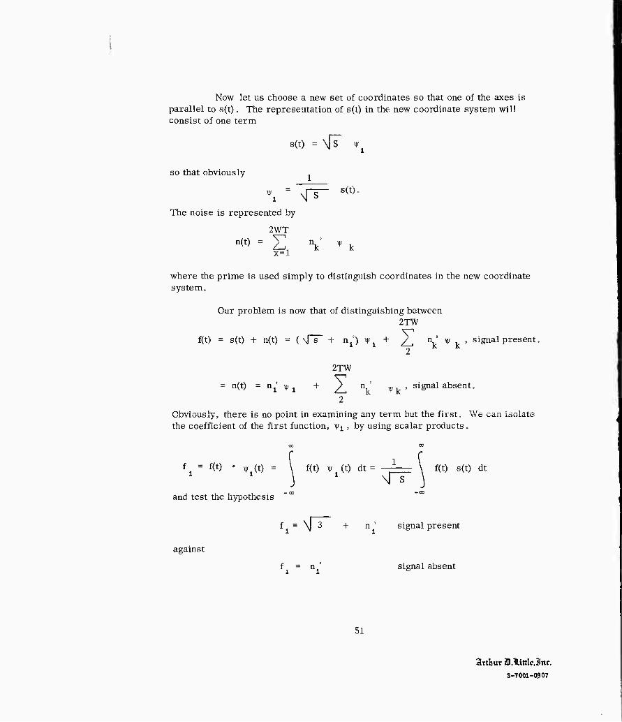
Now let us choose a new set of coordinates so that one of the axes is parallel to s(t). The representation of s(t) in the new coordinate system will consist of one term

s(t) = \JT vi

so that obviously

\ = Nfs" S(t)- The noise is represented by

2WT n(t) = X; nk' w k

x=l

where the prime is used simply to distinguish coordinates in the new coordinate system.

Our problem is now that of distinguishing between 2TW

f(t) = s(t) + n(t) = ( xTs- + n') V, + /_, V ^ ir ' signal Present■

2TW

n(t) = n,' V/1 + ^ n. k ^k

, signal absent.

Obviously, there is no point in examining any term but the first. We can isolate the coefficient of the first function, v1 , by using scalar products.

f = f(t) • w (t) = \ f(t) f (t) dt= -—= f(t) s(t) dt

and test the hypothesis

r^ 3 + n signal present

against

f. = ni' signal absent

51

Arthur ai.HittlcJnr. S-7001-0307

We know that ni is normally distributed aboutzerowith variance N/2just like any among the original components n^, for we assumed a pure rotation of the coordinate system (even though we never explicitly found the new coordinate system). The two distributions are illustrated in Figure 21. The problem is reduced to that of identifying the quantity \[S- when perturbed by a noise with variance N/2. The ratio of the signal to the standard deviation of the noise is

d = ^

\[N/2 = \

2S N

For reliable detection d must be somewhat greater than unity. If the probabil- ity that s(t) will be present is about 50%, and the penalty for missing it when it is present (which we call miss) is the same as the penalty for detecting it when it is not present (which we call false alarm or FA), then we would probably put the threshold of detection near 1/2 \[S. This makes the error probability the same for the two circumstances. They are shown in the first two columns of Table I. In a true search situation, we are searching for a "needle in a hay- stack," and the signal is expected to be absent nearly always. Cutting down the false alarm rate becomes an operational problem, and it is advantageous to raise the threshold. The table shows two examples.

In any case, a value of d of about 5 is needed, and we can nay roughly

\ _2S N

_2S N

_S_ N

32

32N

52

i

SIGNAL PLUS NOISE

FIGURE 21 PROBABILITY DISTRIBUTION OF OUTPUT OF A COHERENT DETECTOR WHOSE INPUT IS WAVEFORMS LIKE THOSE IN FIGURE 20

53

arthur JB.IUttleJnr. S-7001-0207

TABLE I

■

PROBABILITY OF FALSE ALARM ERROR AND OF MISS ERROR AS A FUNCTION OF THRESHOLD LEVEL AND SIGNAL-TO-NOISE RATIO

Threshold 1/2 \| S " XT^ ■ \lN/2 \fr - 2\|N/2

FA Miss FA Miss FA d =\|2S/N Miss

4 2.3 TO'2 2.3 TO"2 1.4 TO*3 1.6 TO"1 2.3T0"2 2.3-10 "2

5 6.2-10"3 6.2T0'? 3.2-10'5 1.6 TO'1 1.4T0"3 2.3-10 "2

6 1.4 TO'3 1.4 TO'3 2.9 TO"7 1.6 TO"1 3.2T0"5 2.3-10'Z

7 2.3 TO'11 2.3 TO"* 2.0T0'9 1.6 TO"1 2.9T0"7 2.3-10-2

8 3.2T0'5 3.2T0'5 2.6T0-12 1.6T0"1 2.0T0"9 2.3-in"2

Let us compare that practical signal-to-noise ratio with the ideal case. Suppose we are concerned with a detection scheme in which there are 1,000,000 cells to look in. If we look and find something, then we have poten- tially distinguished among about 106 possibilities, and receive potentially about 20 bils. We shall, therefore, expect to need

S = 20 x 0.693N = 13.9N

in signal energy.

However, there is error rate to consider. In a detection process, a rather liberal error rate is allowable, say P (e)^-' .01. Referring to the previous- ly quoted formula

- v a C/R P(e)~2 WK

we recall that 2 is the number of binary digits constituting a message; by analogy, v =20. Solving for R/C, one finds

R/C ,41

Hence, the amount of energy required in the signal to achieve an error rate of 0.01 is really

S = 20x 0.693 N/,41 = 33N

54

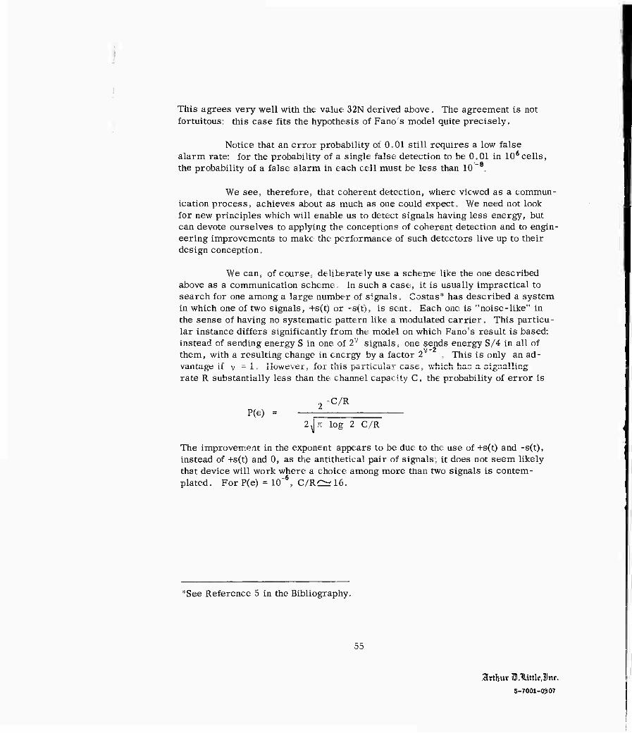
This agrees very well with the value 32N derived above. The agreement is not fortuitous; this case fits the hypothesis of Famrs model quite precisely.

Notice that an error probability of 0.01 still requires a low false alarm rate: for the probability of a single false detection to be 0.01 in 106cells, the probability of a false alarm in each cell must be less than 10 "8.

We see, therefore, that coherent detection, where viewed as a commun- ication process, achieves about as much as one could expect. We need not look for new principles which will enable us to detect signals having less energy, but can devote ourselves to applying the conceptions of coherent detection and to engin- eering improvements to make the performance of such detectors live up to their design conception.

We can, of course, deliberately use a scheme like the one described above as a communication scheme, in such a case, it is usually impractical to search for one among a large number of signals „ Gostas* has described a system in which one of two signals, +s(t) or -s(t), is sent. Each one is "noise-like" in the sense of having no systematic pattern like a modulated carrier. This particu- lar instance differs significantly from the model on which Fano's result is based: instead of sending energy S in one of 2V signals, one sends energy S/4 in all of them, with a resulting change in energy by a factor 2V . This is only an ad- vantage Li v =1. However, for this 'particular case, which has a signalling rate R substantially less than the channel capacity C, the probability of error is

P(e) = 2 C/R

2Jix log 2 C/R

The improvement in the exponent appears to be due to the use of +s(t) and -s(t), instead of -t-s(t) and 0, as the antithetical pair of signals; it does not seem likely that device will work where a choice among more than two signals is contem- plated. ForP(e) = 10"6, C/RC=rl6.

*See Reference 5 in the Bibliography,

55

arthuv B.TUttlcJrtf. S-7001-(Ö07

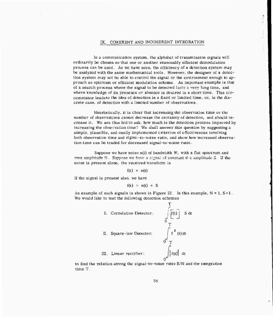
IX. COHERENT AND INCOHERENT INIEGRATION

In a communication system, the alphabet of transmission signals will ordinarily be chosen so that one or another reasonably efficient demodulation process can be used. As we have seen, the efficiency of a detection system may be analyzed with the same mathematical tools. However, the designer of a detec- tion system may not be able to control the signal or the environment enough to ap- proach an optimum or efficient modulation scheme. An important example is that of a search process where the signal to be detected lasts a very long time, and where knowledge of its presence or absence is desired in a short time. This cir- cumstance leadsto the idea of detection in a fixed or limited time, or, in the dis- crete case, of detection with a limited number of observations.

Heuristically, it is clear that increasing the observation time or the number of observations cannot decrease the certainty of detection, and should in- crease it. We are thus led to ask, how much is the detection process improved by increasing the observation time? We shall answer this question by suggesting a simple, plausible, and easily implemented criterion of effectiveness involving both observation time and signal-to-noise ratio, and show how increased observa- tion time can be traded for decreased signal-to-noise ratio.

Suppose we have noise n(t) of bandwidth W, with a flat spectrum and rms amplitude N. Suppose we have a signal of constant d-c amplitude 3. If the noise is present alone, the received waveform is

f(t) = n(t)

If the signal is present also, we have

f(t) = n(t) + S

An example of such signals is shown in Figure 22. In this example, N = 1, S =1. We would like to test the following detection schemes

T r-

i r- _

I. Correlation Detector: |f(t) S dt

II. Square-law Detector:

0 T

f(t)| dt III. Linear rectifier:

to find the relation among the signal-to-noise ratio S/N and the integration time T.

56

First, use the sampling theorem to characterize f(t) as a sequence

f = f(k/2W) k = 1,2, ---, 2TW

n = n(k/2W)

Figure 22 shows how the samples are related to the continuous function f(t). The various samples f^ are independent and have a Gaussian distribution with variance N^ (to avoid another proof, we can define this as Gaussian white noise of band- width W). To a high degree of approximation, we can replace the integrals (with appropriate constant multiplying factors) by sums:

T

I. I

II. 11

III. S III

2TW

A fk- 2w r 5

f(^

1 0 T

2TW fk-

2W | f2(t) dt ^

i J 0

2TW

1

ifkF

T

0

i(t) \*

S dt

We shall devote the rest of the discussion to the sums Sp Sjp and SJJJ,

and try to see how they depend on the integration-time and signal-to-noise ratio. The constant 2W and 2W/S is a scale factor and is not important for the present discussion.

2 Figure 23 shows the samples f^, the squares of the samples f, , and

the absolute values of the samples | ih

Figure 22. for the noise, with and without signal, of

If we look at the signal f(t) at any instant; i.e., if we look at a single sample f, , it has

k

mean value u, s

= S

^0 = 0

variance a 2 s

= N

0o2 = N

if signal present

if signal absent

if signal present

if signal absent

57 3rthur ai.lLittlc.3lnr.

S-7001-W07

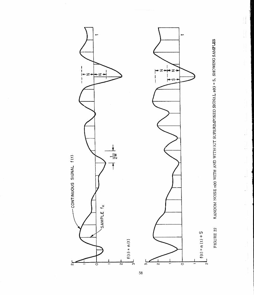
w o

S 8 z

w D Ü

58

O z w

< w

c ii

<M

'in + it c

11

m in

+ c

L. m

,00

Ü

_* >

CD

c

c c II

L_ in

L_ m O

a,

WD

It O

w D < > W H D O

<■

D

W _l a.

C en

-A S

2 o I—t en CL, O

&z

OH ^ S W

< E

CO

W PS D Ü t-H

59 arthur B.lltttlc.ilnr. S-7001-0307

The two variances are the same, and we can ignore the distinction implied by the subscript. We can use (^s - ^o) 1° as a measure of effectiveness of a detection process. For a single sample of the signal, this is just the signal-to- noise ratio S/N. Figure 23a and b shows the samples fjj for the noise and for the signal plus noise shown in Figure 22. Figure 24a shows the sum

5i=S fk = Z <s +v

as a function of 2TW. The expected value of S is p, is

2TWS, and its variance

V Z/s + V| r \

(S + n.) - (2TWS)'

V V (S2 + Sn. + Snk + n n) - (2TWS)2

(2TW)2S2 + 0 + 0 + V nf' - (2TWS)2

V 2

1 nk

= 2TWN

Repeating the computation with S = 0, we find that the mean value and

variance of > n, are M- =0 and o = 2TWN . _, k o o

Figure 25a and b illustrates the distribution of observations to be expected after integration over a time such that 2TW = 20 and 100 respectively. The observations are distributed according to the well-known bell-shaped normal probability distribution. The center of the normal distribution curve is at the expected value |i, and the standard deviation is ö , the square root of the variance. In order to make an effective detector, it is necessary to set a threshold somehow

60

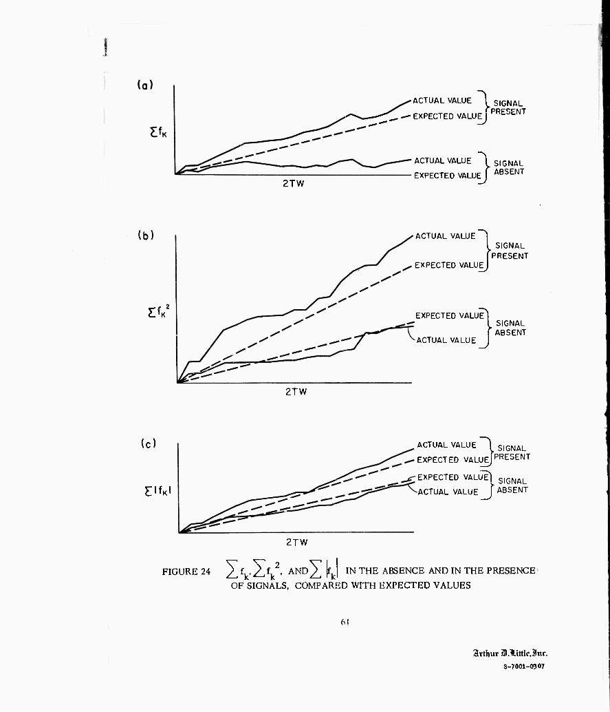
ACTUAL VALUE

—-,'^-. — EXPECTED VALUEJ

l SIGNA r- rPRESE

2TW

ACTUAL VALUE

EXPECTED VALUE

SIGNAL NT

SIGNAL ABSENT

(b)

(c)

vw

ACTUAL VALUE

EXPECTED VALUE

EXPECTED VALUE!

ACTUAL VALUE

SIGNAL PRESENT

SIGNAL ABSENT

2TW

ACTUAL VALUE "^ S|GNAL

EXPECTED VALUEJF,RESENT

EXPECTED VALUT) S|GNAL

ACTUAL VALUE \ ABSENT

2TW

FIGURE 24 2^ fk' 2A2' AND^ LI IN THE ABSENCE AND IN THE PRESENCE'

OF SIGNALS, COMPARED WITH EXPECTED VALUES

atthur ZD.llttleJttc.

S-7001-0307

to

o 8

<t-i

o

in CM

W Pi 5 Ü [I-

62

so that an observation will nearly always fall on one side of the threshold when the signal is present, and nearly always fall on the other side of the threshold where the signal is absent. Inasmuch as the probability distributions overlap (the overlapping part is cross-hatched in the figure), there is no place to establish a threshold which will give error-free results. A reasonable and useful measure of the effectiveness is the ratio of the distance between the peaks, n s - |i o. and the width of the peak, measured by a . When only one sample is taken, we have seen that the ratio is S/N. When 2TW samples are integrated in a coherent detector, the measure of effectiveness is

's " "o 2TWS-0 =v^ S

TirwN 2 N

i.e., the effect of integration over time T is equal to the effect of improving the S/N ratio by a factor V 2TW.

2 2 In a square-law detector, the sample is squared to get i^ = nj, or

(nj, + S) (Figure 23c and d). Let us examine the build-up of the sum,

S £ = /_, (s + nk)2 ~ / (S2 + 2S\ + nD (signal present)

or = ) n* (signal absent)

2 2 Its expected value is 2TWS + 2TWN if the signal is present, and

2TWN2 if the signal is absent

_ o _JV for both cases. Figure 24b shows the actual growth of ^ f^ compared with the expected value.

We could find the variance of SJJ by brute force. However, it is easier to work indirectly, and to define a new population whose members are

zk = S2+2Snk + nk

2

and find sample mean and sample variance, and work indirectly to the sums.

If we define

nv = Nxk

63

artbur l.llittlejnr.

S-7001-0307

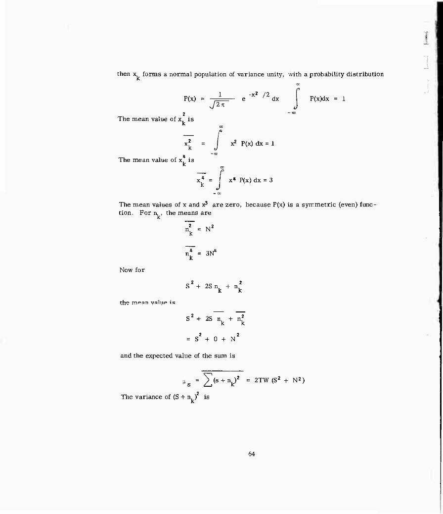
then x^ forms a normal population of variance unity, with a probability distribution cc

P(x) = J__ e 'x2 /2 dx P(x)dx = 1 J^ J

2 The mean value of x, is

k

.2 Xk = J x2 P(X) ^= 1

4 The mean value of x, is

k — P x* = j x» P(x) dx = 3 k J

- oc

The mean values of x and x3 are zero, because P(x) is a syrrmetric (even) func- tion. For n, , the means are

K

Z= N2 k

Z= 3N4 k

Now for

tVip» mpqn valiip is

S2 + 2S n, + n,2

k k

S2 + 2S n, + nf k k

2 2 = S + 0 + N

and the expected value of the sum is

h s ^(s + n^2 = 2TW (S2 + N2)

2 The variance of (S + n ) is

64

YJ{s+\y' - (S+V22

U3 22 3422 S + 4S n + 6S n 4- 4SIL, + n' - (S + N )

4 2 2 tt U 2 _2 U = S + 0 + 6S N + 0 + 3N - S - 2S >r - N

= 4S2N2 + 2N4

Hence the variance of the sum is

n2 = V (S + n?) =2TW(4S2N2 + 2N4) as / . k

By repeating the computation with S = 0, we can find

M, = 2TWN2

0

2 = 2TWN'1

o o

Figure 25c and d shows normal distribution curves with these means and variances for 2TW = 20 and 100.

An aggravating factor here is that the variance is different when the signal is present than it is when the signal is absent. Let us agree that we are most inter- ested in the case S/N < < 1. Then

2TW(4S2N2 + 2N4)r^2TW • 2N4 = 4TWN'1

independent of whether the signal is present.

Using the same criterion as before, we measure the effectiveness of the detector by

ls "u o _ 2TW [j(S2 + N2 ) - (N2 fl _ fs N 4~™

i.e., integrating a time T is equivalent to improving S/N by a factor 4/ TW.

65

Arthur l.HittlcJnr. S-7001-0307

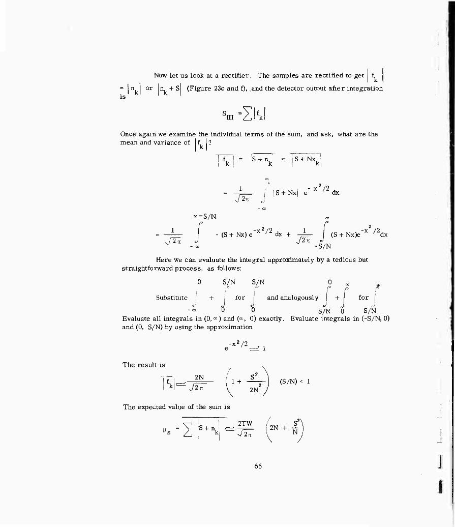
_ n, 1 or n, + S kl k IS

Now let us look at a rectifier. The samples are rectified to get 1

(Figure 23c and f), and the detector output after integration

SIII

=SKI Once again we examine the individual terms of the sum, and ask, what are the mean and variance of f

k?

f = S + n = ! S + Nx, ! I k i k ki

J2K J - x /2

! S + Nxi e ' dx

x=S/N

^J2n

- (S + Nx)e'x2/2 dx + -L- (S + Nx)e'X /2dx J2n J

-S/N

Here we can evaluate the integral approximately by a tedious but straightforward process, as follows:

0 S/N S/N 0

Substitute + j for and analogously + for

0 S/N 0 S/N Evaluate all integrals in (0, <=) and {<*>, 0) exactly. Evaluate integrals in (-S/N, 0) and (0, S/N) by using the approximation

e-x2/2^ 1

The result is

2N

i kl~" J2K \

The expected value of the sum is

1 + 2N

(S/N) < 1

!S + n. 2TW //1XT S

2N

-1=- 2N + TTF

V

66

when the signal is present, and

|i = / I n o Z-J k

2TW

'in' 2N

when the signal is absent. The difference is

2TW S "' N s/2Tt

What about the variance? The mean square value is easy to evaluate; for the absolute value operation is trivial when the function is squared:

S + n, 2 2 2

(S + n ) = S + N

One must be careful not to jump to conclusions, however. The mean val". laboriously computed above must now be used.

var v i S + n, n k

) S + n, S + n,

2 2 -y S + N

4N 2n

4S 1 S 2 it 2^ 2

N

2N 2TW S' + N

If S/N < < 1, this is approximately

0 2 — 2TWN2 (1-1)

Similarly

2TWN (1 - -)

2S

2 KN

These probability distributions are plotted in Figure 25e and f for 2TW = 20 and 100.

67

arthur ai.HittlcJnr. S-7001-0307

The measure of merit of the detector is

^S " ^0 2TWS

S N

Jin ■ 0

x/zTW ,.1). N

/ ( s J TW \ N <7 K - 2 /

i.e., the effect of integration for a time T is equivalent to the effect of improving

S . .. , / TW

— by a factor 4/ —

Note that this is just a shade worse than 4/ TV/.

The ratio is 4/ -—" or approximately 0.1 db.

Table II summarizes the expected values and variances of the outputs of these three kinds of detectors. The effect of integration with a coherent deteccor over a time T is equivalent to an improvement in the input signal-to- noise ratio of a factor \/2TW. This is sometimes stated as 3 db improvement per doubling of integration time. The effect of integration with an incoherent square-law or linear rectifier detector over a time T is equivalent (when the

input S/N is low) to an improvement in the signal-to-noise ratio of 4/ TW or

4/ TW/(TI - 2) respectively. This is sometimes stated as 1.5 db improvement per doubling of integration time .

There is another respect in which the square-law and linear rectifier detectors are inferior to the coherent detector. The distributions in Figure 25 and in Table II show that the expected value of the output of a coherent detector depends on the signal only, and the variances on the noise only; whereas in square-law and linear rectifier detectors the expected values and variances de- pend jointly on signal and noise. Now to a first approximation, the best place to put the detection threshold depends on the expected value of the output, and not on the variance. This means that the threshold can be set in a coherent detector independent of the noise. This is not possible in linear or square-law detectors, for the output wanders back and forth as the noise level varies. Unless the noise is very uniform, as, for example, is thermal noise in a low-noise electronic amplifier, some extra provision must be made to compensate for secular varia- tions in noise level.

68

<

O

o

h

w CO

&< o

PL,

H D O w S

O w u z < < > Q 2 < W D

Q w H U w

1 M 1 St 2

Ü3 fc' ^^. CN

=f .-k z cslt- (N 1

(U CM .—1

B 'z + •t-t u

eg

2 CM

rt CN + > CM CM C/3

1 - 1 w 1 1

T3 0) *-J 0) O 3 (U ■—i

& > W

to

IM

0) CM

H 2 2 ^ u h

>1 al (N

^1 > s O 0) CO

-^H o 2 ■a

0) -t-j OJ u 3 a) a X

al > o

m

H IN

2

2

2

o

co|2 + 2

<N| t

2

H CM

/

h 0 ^J

o

o a) 4-)

VH u D O (U j-) 4-J H

B S 4^

ä ^ o i—i a) 0)

S ►J öS F 0) M )H )H aj ü tD Ä ^3 d O cr U CO 3

69

arthur Zn.lUttlcJnr. S-7001-O?07

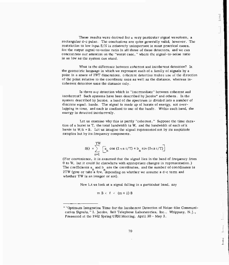
These results were derived for a very particular signal waveform, a rectangular d-c pulse. The conclusions are quite generally valid, however. The restriction to low input S/N is relatively unimportant in most practical cases, for the output signal-to-noise ratio in all three of these detectors, and we can concentrate our attention on the "worst case, " where the signal-to-noise ratio is as low as the system can stand.

What is the difference between coherent and incoherent detection? In the geometric language in which we represent each of a family of signals by a point in a space of 2WT dimensions., coherent detection makes use of the direction of the point relative to the coordinate axes as well as the distance, whereas in- coherent detection uses the distance only.

Is there any detection which is "intermediate" between coherent and incoherent? Such systems have been described by Jacobs* and others. In the system described by Jacobs, a band of the spectrum is divided into a number of discrete equal bands. The signal is made up of bursts of energy, not over- lapping in time, and each is confined to one of the bands. Within each band, the energy is detected incoherently.

Let us examine why this is partly "coherent." Suppose the time dura- tion of a burst is T, the total bandwidth is W, and the bandwidth of each of k bands is W/k = B. Let us imagine the signal represented not by its amplitude samples but by its frequency components .

TW

f(t) = > fa cos (2 it n t/T) + b sin(2rrnt/T) / , I n n -J n=l

(For convenience, it is assumed that the signal lies in the band of frequency from 0 to W, but it could lie elsewhere with appropriate changes in representation.) The coefficients a and b are the coordinates, and the number of coordinates is

n n 2TW (give or take a few, depending on whether we assume a d-c term and whether TW is an integer or not).

Now let us look at a signal falling in a particular band, say

mB< f < (m + l)B

* "Optimum Integration Time for the Incoherent Detection of Noise-like Communi- cation Signals, " I. Jacobs, Bell Telephone Laboratories, Inc., Whippany, N.J., Presented at the 1962 Spring URSI Meeting, April 30 - May 3.

70

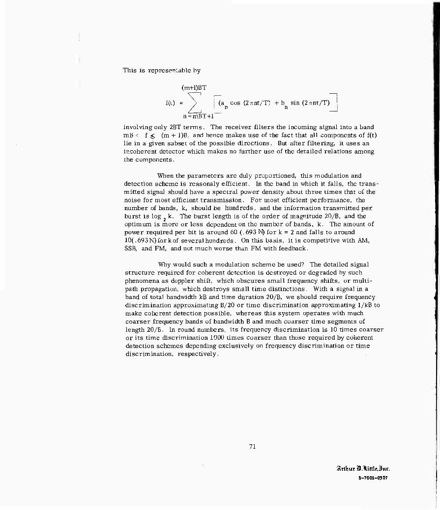
This is represenlable by

(m+l)BT

1(0 = ) j (a cos (2 7xnt/rn +b sin (2 rnit/T) ' ■ D n

n = mB r+1

involving only 2BT terms. The receiver filters the incoming signal into a band mB < f ^ (m + 1)B; and hence makes use of the fact that all components of f(t) lie in a given subset of the possible directions. But after filtering, it uses an incoherent detector which makes no further use of the detailed relations among the components.

When the parameters are duly proportioned, this modulation and detection scheme is reasonaly efficient. In the band in which it falls, the trans- mitted signal should have a spectral power density about three times that of the noise for most efficient transmission. For most efficient performance, the number of bands, k, should be hundreds, and the information transmitted per burst is log k. The burst length is of the order of magnitude 20/B, and the optimum is more or less dependent on the number of bands, k. The amount of power required per bit is around 60 (.693 N) for k = 2 and falls to around 10( .693N)forkof several hundreds. On this basis, it is competitive with AM, SSB, and FM, and not much worse than FM with feedback.

Why would such a modulation scheme be used? The detailed signal structure required for coherent detection is destroyed or degraded by such phenomena as doppler shift, which obscures small frequency shifts, or multi- path propagation, which destroys small time distinctions. With a signal in a band of total bandwidth kB and time duration 20/B, we should require frequency discrimination approximating B/20 or time discrimination approximating 1/kB to make coherent detection possible, whereas this system operates with much coarser frequency bands of bandwidth B and much coarser time segments of length 20/B. In round numbers, its frequency discrimination is 10 times coarser or its time discrimination 1000 times coarser than those required by coherent detection schemes depending exclusively on frequency discrimination or time discrimination, respectively.

71

Arthur Zn.lLittlcJnr. S-7001-0307

X. CONCLUSION

Where, now, has this comparison of modulation and detection systems brought us? It has been shown that there is a minimum average energy required to transmit one bit of information in the presence of random noise of fixed in- tensity and uniform spectral distribution. The degree to which amplitude modu- lation, single-sideband modulation, frequency modulation, frequency modulation with feedback, and a particular frequency-band-limited noise-pulse modulation system approach the ideal has been estimated, and all were found to require three to 100 times more energy per bit than the ideal minimum. Detection of a signal in a noisy background , as in a radar, was viewed as a communication process, and it was found that the energy required per bit of effective informa- tion received is only slightly more than the ideal minimum.

Implicitly, we have seen how to encode an information-carrying signal of relatively narrow bandwidth and high signal-to-noise ratio in a new form having broad bandwidth and low signal-to-noise ratio. When the formula for channel capacity was developed, it became obvious at once that channels having a high signal-to-noise ratio used more power than is necessary to transmit their information. On the other hand, for a communication channel to be use- ful to the ultimate users, the received message must have a relatively high rnessage-to-noise ratio, that is, the error rate must be low. In all of the more straightforward and naive ways of modulating and demodulating, the signal is so much like the message that to keep a high message-to-noise ratio, we must have a high signal-to-noise ratio.

The derivation we gave of the channel-capacity formula suggests one relatively complex way to signal through a noisy channel without introducing errors into the message: by using almost countless numbers of noise-like wave- forms as an alphabet of digital signals. This solution to the problem is con- ceptually easy to handle, and on paper allows us to reach significant results. However, everyone seems to agree that this is an undesirable way to modulate and demodulate, or to code and decode, because it would require extremely complex equipment. But now frequency-modulation-with-feedback is a way of making a trade among bandwidth, power,and signal-to-noise ratio which does not involve resorting to complicated digital codes.

Other advantages besides saving of transmitter power arise from the efficient use of a communication channel. For example, if we consider the efficient utilization of space in our signal-space of 2WT dimensions, we realize that in signal-space any noise is as good as any signal, and no signal is any better than any noise. Thus, we find that in such a contextit is impossible to have especially obnoxious jamming signals. There is no more efficient signal

72

I

for jamming than random noise, and we already know that under these circum- stances the system can be designed to operate with a very low signal-to-noise ratio. We can see that to jam such a system successfully, we must put into the receiver more jamming power than signal power. This makes jamming costly.

There is another benefit from operating with a very low signal-to-noise ratio. If we can really work a communications system so that the signal power- level is much lower than the noise power-level, we introduce the poösibility of signalling in such a way that it is hard to tell whether any signal is being trans - mitted at all. We can thus indirectly make the jamming problem more diffi- cult again, for the jammer must first hunt around to find out where there is something to jam before he knows whether to waste his effort trying to jam it.

By looking at seaching for the presence of a signal as a communication process, we have learned that there is a limit to the detectibility of a single signal in a noise background, and that this limit is described in terms of. the noise, energy density and the received signal energy. The shape of the signal wave is not significant as long as it is fully known in advance to the detector. The process of measuring the correlation between the known signal waveform and the received wave is known as coherent detection. If the signal waveshape is not completely known, certain kinds of incoherent detection, which vary according to the degree of ignorance of the signal waveshape, are possible. The less that is known about the signal waveshape, the more signal energy is required to assure positive detection. If the signal is a single pulse or a burst of a sinusoidal wave, one can use very simple detectors which approach the theoretical limit of search performance. Many signals which at first contact appear to be quite specific, such as, for example, the acoustic signal resulting from the spoken sound "ee," do in fact vary over a wide range, and are corre- spondingly hard to detect reliably.

In summary, the ultimate limit to the rate of transmission of informa- tion in a noisy background, or to the detection of a signal in a noisy background, is primarily determined by the noise power density and the signal power or energy. To approach this theoretical limit, the receiver must have precise de- tailed knowledge of the possible waveshapes of the transmitted signal. In the absence of such knowledge, more signalling power or energy is required.

73

Arthur JDAittlcJnr. S-7001-0307

BIBLIOGRAPHY

1. "Communication in the Presence of Noise," C. E. Shannon, Proc. LR.E., Vol. 47, No. 1, January 1959, pp. 10-21.

2. "An Outline of Information Theory," E. N. Gilbert, The American Statistician, Vol. 12, February 1958, pp. 13-19.

3. "Interplanetary Communications," J. R. Pierce and C, C. Cutler, Advances in Space Science, Vol. 1, ed. by F. I. Ordway, III, Academic Press, 1959.

4. Transmission of Information, Robert M. Fano, MIT Press and John Wiley & Sons, New York, 1961. .

5. "Poisson, Shannon and the Radio Amateur," J. P. Costas, Proc. I.R.E., Vol. 47, No. 12, pp. 2058-2068, December 1959.

6. "Prediction and Entropy of Printed English," C. E. Shannon, Bell System Technical Journal, Vol. 30(1951), pp. 50-64.

74

i

DISTRIBUTION LIST

No. of Copies

Bureau of Ships, Code 370 10 Department of the Navy Washington 25, D.C.

Chief of Navai Operations (OP-71) 10 Department of the Navy Washington 25, D.C.

Commanding Officer & Director 4 U.S. Navy Underwater Sound Laboratory Fort Trumbull, New London, Conn.

Attn: Mr. H. E. Nash

Office of Naval Research, Code 400X 2 Department of the Navy Washington 25, D C.

Director 2 U.S. Naval Research Laboratory Washington 25, D.C.

Attn: Dr. H. Saxton

Chief, Bureau of Naval Weapons 2 Department of the Navy Washington 25, D.C.

Attn: Mr. I. H. Gatzke

Commanding Officer 2 U.S. Naval Air Development Center Johnsville, Pa.

Attn: Mr. R. I. Mason

Commanding Officer & Director 2 U S. Navy Electronics Laboratory San Diego 52, California

Attn: Dr. D. A. Wilson

75

artbur JJ.TUttlcJnc S-7001-0307

Commander, Antisubmarine Warfare Force U. S. Pacific Fleet Navy No. 128, c/o FPO San Francisco, California

Marine Physical Laboratory of the Scripps Institution of Oceanography

San Diego 52, California

Technical Library (Code P80962) U.S. Naval Ordnance Test Station Pasadena Annex 3202 East Foothill Blvd. Pasadena 8, California

Officer in Charge U.S. Naval Oceanographic Unit Building #1, Treasure Island San Francisco 30, California

Commander Oceanographic System Atlantic Norfolk 11, Virginia

Commander, Antisubmarine Warfare Force U.S. Atlantic Fleet Norfolk 11, Virginia

Commanding Officer U.S. Navy Underwater Sound Laboratory Research Detachment Navy No. 138, c/o FPO New York, N. Y.

Attn: Dr. W. A. Von Winkle

Hudson Laboratories P. O. Box 239 Dobbs Ferry, N. Y.

Attn: Dr. R. A. Frosch

No. of Copies

2

76

No. of Copies

President Naval War College Newport, Rhode Island

Commander Destroyer Development Group Two U. S. Atlantic Fleet Newport, Rhode Island

Director of Research Institute of Naval Studies 185 Ale wife Brook Parkway Cambridge 38, Mass.

Director, ASW Systems Analysis Group Undersea Warfare R&D Planning Council U.S. Naval Ordnance Laboratory White Oak, Silver Spring, Md.

77

Arthur ZD.HittlcJInr. S-7001-OJ07

PROJECT TRIDENT TECHNICAL REPORTS

Report No. Title

1011260 COLOSSUS I, December, 1960 (C)

1021260 THEORETICAL INVESTIGATION OF CROSS-FIX PROBLEMS AND CORRELATION EFFECTS, December, 1960 (C)

1031260 THE SUBMARINE AS A SURVEILLANCE PLATFORM, Dec- ember, 1960 (S)

1041260 Title Classified, December, 1960 (S)

1051260 AIRBORNE JEZEBEL, December, 1960 (S)

1061260 SURFACE-SHIP SONARS IN OCEAN-AREA SURVEILLANCE, December, 1960 (S)

1071260 Title Classified, December, 1960 (S)

1080361 LOW-POWER ENERGY SOURCES, March, 1961 (C)

1090561 SOLUS, May, 1961 (C)

1100561 NONACOUSTIC METHODS FOR SUBMARINE DETECTION, May, 1961 (S)

1110561 ARTEMIS, May, 1961 (S)

1120561 COLOSSUS II, May, 1961 (S)

1130961 RELIABILITY OF UNATTENDED ELECTRONICS EQUIPMENT, September, 1961 (U)

1141061 NUTMEG, October, 1961 (S)

1150162 DEEP JULIE, January, 1962 (S)

1160262 METHODS FOR ANALYZING THE PERFORMANCE OF DIS- TRIBUTED FIELDS OF DETECTORS, February, 196z (C)

1170262 MAGNETIC ANOMALY DETECTORS IN FIXED SHALLOW WATER BARRIERS, February, 1962 (S)

79

atthur ZDAlttlcJnr. S-7001-0307

Report No. Title

1180262 ELECTRICAL CONDUCTIVITY, COMPRESSIBILITY, AND VISCOSITY OF AQUEOUS ELECTROLYTIC SOLUTIONS, February, 1962 (U)

1190462 A FEASIBILITY STUDY OF THE PASSIVE DETECTION OF QUIET SUBMARINES, April, 1962 (S)

1200562 Title Classified, May, 1962 (S)

1210562 RADIATED NOISE CHARACTERISTICS OF DIESEL-ELEC- TRIC SUBMARINES, May, 1962 (S)

1220562 DIRECTIVE RECEIVING ARRAYS, May, 1962 (C)

1230662 ANALYTICAL BACKGROUND OF COMPUTATIONAL METHODS FOR UNDERWATER SOUND PROPAGATION, June, 1962 (U)

1240762 MARINE CORROSION AND FOULING, July, 1962 (U)

1250862 SURVEY ON AMBIENT SEA NOISE, August, 1962 (C)

1260862 DEEP SUBMERSIBLE WORK VEHICLES, August, 1962(C)

1270862 THE EFFECT OF PRESSURE ON THE ELECTRICAL CON- DUCTIVITY OF SEA WATER, August, 1962 (U)

.1 n81262 ENGINEERING PROPERTIES OF MARINE SEDIMENTS, December, 1962 (U)

80

I 1

9^

0) p

o S

11 I a

11

3 D T]

5 I

B2

Z H o w

E a

.'•a 8

1

0 si, e

o a H ö ID q . U

aj 4i g a»

■S s § ^ ) y « m a

! I I I S !■§" g i

■ ill I III I

Ü OD M

§•3'S a

" y

8.9 S| ä 3 SI" IK

&•§,

PI pH Ö

«i 5 " s

e-S ä a •all 8« S

a a

P s rs

ä a u *,

.III' a -a S J8 j

8 & ü a «!

■a -o.

Jj s

r ~i

o

b

I "I a w U fi s

o

" 1 -a 3- IBS- 8 M TJ B 3 ^ s -S

I ä a g II • " I«

81

1^ a E 3< jj

3 3 S f 3 v p

--v "an

frl s a I 3 ■ s - = 1 I all

&s s

o 2 n

a |§|s

sis H &. "o

01 s O -J 4J

III Q) 5 u s S .a

ill

L3 fi ■3 i .

ill