Relationship between local and global modulus of...
12
ORIGINALS ORIGINALARBEITEN Relationship between local and global modulus of elasticity in bending and its consequence on structural timber grading Michela Nocetti • Loı ¨c Brancheriau • Martin Bacher • Michele Brunetti • Alan Crivellaro Received: 19 June 2012 / Published online: 1 March 2013 Ó Springer-Verlag Berlin Heidelberg 2013 Abstract The study analyses the relationship between local and global modulus of elasticity and develops and evaluates different models to predict local from global modulus measurements. The mechanical tests were per- formed on four species commonly used in Italy for struc- tural purposes: fir, Douglas-fir, Corsican pine and chestnut. Two or three cross-sections and two provenances were sampled for each species. A theoretical analysis showed that the local–global modulus relationship was of polyno- mial form with only one coefficient. The effect of the species on the relationship was significant as well as the cross-section but only for softwoods. The effect of the cross-section was explained by the presence and the size of defects in the mid span. The different models were applied and then compared by means of the optimum grading: only slight differences among models emerged. Although optimum grading was strongly dependent on the sampling and on the grade combination, for softwoods the model for species and section showed very similar results to the grading with the true local modulus; inclusion of the knot values in the model led to only slight improvements. For chestnut all models were found to be comparable. Zusammenhang zwischen lokalem und globalem Biege-E-Modul und dessen Auswirkung auf die Festigkeitssortierung Zusammenfassung Diese Studie untersucht den Zusam- menhang zwischen lokalem und globalem E-Modul von Schnittholz und entwickelt und vergleicht verschiedene Modelle, um den lokalen E-Modul aus globalen Messun- gen zu bestimmen. Die Versuche wurden an vier in Italien ha ¨ufig als Bauholz verwendeten Holzarten durchgefu ¨hrt: Tanne, Douglasie, Korsische Schwarzkiefer und Edelkast- anie. Je Holzart wurden zwei oder drei Querschnitte aus jeweils zwei Wuchsgebieten beschafft. Eine theoretische Untersuchung zeigte, dass der Zusammenhang zwischen lokalem und globalem E-Modul einer Polynom-Funktion mit nur einem Koeffizienten entspricht. Signifikanten Einfluss auf den Zusammenhang hatte die Holzart und bei Nadelho ¨lzern auch der Querschnitt, was durch das Vorhandensein und die Gro ¨ße der A ¨ ste im mittleren Pru ¨f- bereich begru ¨ndet wurde. Die verschiedenen Modelle wurden angewandt und bezu ¨glich ihrer Auswirkung auf die optimale Sortierung verglichen: Es zeigten sich nur geringe Unterschiede. Obwohl die optimale Sortierung sehr stark von der Probenahme und der Sortierklassen-Kombination abhing, fu ¨hrte das Modell auf Basis von Holzart und Querschnitt bei den Nadelho ¨lzern zu sehr a ¨hnlichen Ergebnissen wie eine Sortierung nach dem gemessenen lokalen E-Modul; die Beru ¨cksichtigung der Astwerte fu ¨hrte M. Nocetti (&) M. Brunetti CNR-IVALSA, Istituto per la Valorizzazione del Legno e delle Specie Arboree, Via Madonna del Piano 10, 50019 Sesto Fiorentino (FI), Italy e-mail: [email protected] L. Brancheriau CIRAD-De ´partement PERSYST, Performances des syste `mes de production et de transformation tropicaux, UPR 40 Production et valorisation des bois tropicaux, TA B-40/16, 73 Rue Jean Franc ¸ois Breton, 34398 Montpellier Cedex 5, France M. Bacher MiCROTEC Srl, Via Julius Durst Straße 98, 39042 Bressanone, Italy A. Crivellaro Department of Land, Environment, Agriculture and Forestry, University of Padova, Viale dell’Universita ` 16, 35020 Legnaro (PD), Italy 123 Eur. J. Wood Prod. (2013) 71:297–308 DOI 10.1007/s00107-013-0682-7
Transcript of Relationship between local and global modulus of...
ORIGINALS ORIGINALARBEITEN
Relationship between local and global modulus of elasticityin bending and its consequence on structural timber grading
Michela Nocetti • Loıc Brancheriau •
Martin Bacher • Michele Brunetti • Alan Crivellaro
Received: 19 June 2012 / Published online: 1 March 2013! Springer-Verlag Berlin Heidelberg 2013
Abstract The study analyses the relationship betweenlocal and global modulus of elasticity and develops and
evaluates different models to predict local from global
modulus measurements. The mechanical tests were per-formed on four species commonly used in Italy for struc-
tural purposes: fir, Douglas-fir, Corsican pine and chestnut.
Two or three cross-sections and two provenances weresampled for each species. A theoretical analysis showed
that the local–global modulus relationship was of polyno-
mial form with only one coefficient. The effect of thespecies on the relationship was significant as well as the
cross-section but only for softwoods. The effect of the
cross-section was explained by the presence and the size ofdefects in the mid span. The different models were applied
and then compared by means of the optimum grading:
only slight differences among models emerged. Although
optimum grading was strongly dependent on the samplingand on the grade combination, for softwoods the model for
species and section showed very similar results to the
grading with the true local modulus; inclusion of the knotvalues in the model led to only slight improvements. For
chestnut all models were found to be comparable.
Zusammenhang zwischen lokalem undglobalem Biege-E-Modul und dessenAuswirkung auf die Festigkeitssortierung
Zusammenfassung Diese Studie untersucht den Zusam-
menhang zwischen lokalem und globalem E-Modul vonSchnittholz und entwickelt und vergleicht verschiedene
Modelle, um den lokalen E-Modul aus globalen Messun-
gen zu bestimmen. Die Versuche wurden an vier in Italienhaufig als Bauholz verwendeten Holzarten durchgefuhrt:
Tanne, Douglasie, Korsische Schwarzkiefer und Edelkast-
anie. Je Holzart wurden zwei oder drei Querschnitte ausjeweils zwei Wuchsgebieten beschafft. Eine theoretische
Untersuchung zeigte, dass der Zusammenhang zwischenlokalem und globalem E-Modul einer Polynom-Funktion
mit nur einem Koeffizienten entspricht. Signifikanten
Einfluss auf den Zusammenhang hatte die Holzart und beiNadelholzern auch der Querschnitt, was durch das
Vorhandensein und die Große der Aste im mittleren Pruf-
bereich begrundet wurde. Die verschiedenen Modellewurden angewandt und bezuglich ihrer Auswirkung auf die
optimale Sortierung verglichen: Es zeigten sich nur geringe
Unterschiede. Obwohl die optimale Sortierung sehr starkvon der Probenahme und der Sortierklassen-Kombination
abhing, fuhrte das Modell auf Basis von Holzart und
Querschnitt bei den Nadelholzern zu sehr ahnlichenErgebnissen wie eine Sortierung nach dem gemessenen
lokalen E-Modul; die Berucksichtigung der Astwerte fuhrte
M. Nocetti (&) ! M. BrunettiCNR-IVALSA, Istituto per la Valorizzazione del Legno e delleSpecie Arboree, Via Madonna del Piano 10, 50019 SestoFiorentino (FI), Italye-mail: [email protected]
L. BrancheriauCIRAD-Departement PERSYST, Performances des systemes deproduction et de transformation tropicaux, UPR 40 Production etvalorisation des bois tropicaux, TA B-40/16, 73 Rue JeanFrancois Breton, 34398 Montpellier Cedex 5, France
M. BacherMiCROTEC Srl, Via Julius Durst Straße 98,39042 Bressanone, Italy
A. CrivellaroDepartment of Land, Environment, Agriculture and Forestry,University of Padova, Viale dell’Universita 16,35020 Legnaro (PD), Italy
123
Eur. J. Wood Prod. (2013) 71:297–308
DOI 10.1007/s00107-013-0682-7
nur zu geringen Verbesserungen. Fur die Edelkastanie
waren alle Modelle vergleichbar.
1 Introduction
The standard EN 338 (2009) defines timber strength classesapplied when designing structures. The modulus of elas-
ticity is one of the three wood properties (together with
bending strength and wood density) used to allocate singletimber elements to the strength classes. An accurate mod-
ulus of elasticity measurement is therefore essential to use
timber properly: an overestimation could lead to unsafestructures, while an underestimation to yield losses.
The standard EN 408 (2012) provides two methods for
the determination of the static modulus of elasticity inbending, defined as local (Elocal) and global (Eglobal)
modulus, and both methods have advantages and disad-
vantages. In the Elocal determination method the mid-spandeflection is measured. It represents the pure bending
deflection (no shear effect), but it is also subject to higher
risks of measurement errors due to the reference points fordeflection measurement, initial specimen twist and, mainly,
due to the little deflection size (Bostrom et al. 1996; Solli
1996; Bostrom 1997; Kallsner and Ormarsson 1999; Solli2000). Besides, the Elocal is measured in the third span and
considers only a small part of the test specimen volume
(Bogensperger et al. 2006). The Eglobal determinationmethod provides the measurement of the total deflection,
which is representative of the whole span, less subject to
measurement errors (although it may include higherdeflection measures due to the local indentation at the
loading points), but it combines bending and shear defor-
mation (Solli 2000).Previous studies investigated the relationship between
local and global modulus. Bostrom (1999) found an effect
of the shear deformation, the specimen depth and the woodquality (critical defect) on the relationship between local
and global modulus in Norway spruce and Scots pine from
Sweden. For high values of the modulus of elasticity, Elocal
was higher than Eglobal, the opposite for low values; the
ratio Elocal/Eglobal was mainly affected by shear deforma-
tions for large dimension specimens, while for smalldimension timber there was a greater influence of the
critical defect on Elocal than Eglobal. Holmqvist and
Bostrom (2000) and Solli (2000) reported similar resultsfor Norway spruce. The linear models were: Elocal =
1.13 9 Eglobal - 800 (R2 = 0.82, N = 800, Holmqvist
and Bostrom 2000) and Elocal = 1.18 9 Eglobal - 856(R2 = 0.89, N = 200, Solli 2000). Denzler et al. (2008)
showed that in spruce the ratio Elocal/Eglobal was above theunity for high values of modulus of elasticity and below the
unity for low values in spruce. The regression model for
spruce was: Elocal = 1.224 9 Eglobal - 1,584 (R2 = 0.90;
N = 3491). On the contrary Ravenshorst and van deKuilen (2009) showed a very constant relationship between
Elocal and Eglobal both for spruce, some tropical hardwoods
and chestnut, while no effect of depth was reported. Theregression model for the 1,354 specimens was: Eloca-
l = 1.16 9 Eglobal - 257 (R2 = 0.88; spruce N = 601,
chestnut N = 300, cumaru N = 192, massarandubaN = 54, purpleheart N = 45, tauari vermelho N = 51 and
azobe N = 111). Finally, Ridley-Ellis et al. (2009) mea-sured both bending modulus of elasticity and shear mod-
ulus in specimen of Sitka spruce and concluded that the
main reason of the difference between Elocal and Eglobal
was the high variability of Elocal within the specimen, not
shear deformation.
The determination of the characteristic values of struc-tural timber (EN 384 2010) provides the measurement of
Eglobal for the modulus of elasticity and the following
conversion equation to pure bending modulus (EEN384) isapplied: EEN384 = 1.3 9 Eglobal - 2,690. Such equation
was tested for Central European species and it seemed to
underestimate Elocal, independently by size, species(spruce, pine, Douglas-fir and larch were analysed), nor
wood quality. However, the difference was considered
marginal and the authors suggested to keep the EN 384equation unchanged (Denzler et al. 2008). Bogensperger
et al. (2006), on the contrary, discussed the mechanical
inconsistency of the EN384 linear equation and proposedthe substitution by a hyperbolic function. Nevertheless,
most of the cited studies were concerned with Central or
Northern European species and provenances. The aim ofthis study was thus (a) to analyse the effects of species, size
and wood quality over the relationship between Elocal and
Eglobal for structural timber of Italian provenances; (b) todevelop models that include such factors, aimed to predict
Elocal from Eglobal measurements; (c) to evaluate the
models and, thus, to verify the fitting of EN384 conversionequation to South Europe timber.
2 Materials and methods
2.1 Sampling
Tests were performed on a total of 1,939 specimens of four
species: fir (Abies alba Mill.—ABAL) and Douglas-fir(Pseudotsuga menziesii Franco—PSMN) sampled in cen-
tral Italy; Corsican pine (Pinus nigra Arnold subsp. laricio(Poir.) Maire—PNNL) and chestnut (Castanea sativaMill.—CTST) sampled in southern Italy. For each species
2 or 3 cross-sections and 2 provenances were sampled. The
number of specimens grouped by species and size isreported in Table 1 (Nocetti et al. 2010).
298 Eur. J. Wood Prod. (2013) 71:297–308
123
2.2 Methods
After kiln-drying to a nominal moisture content of 12 %,
the knot characteristics of each specimen were recorded bymeans of GoldenEye (MiCROTEC Srl). The machine uses
X-ray technology to detect the presence of each knot in the
timber element and measures knot dimension and positionand returns a ‘‘knot parameter’’ (KN) calculated by an
algorithm that combines the projected knot area over a
window length of 150 mm and the knot position. Thegreater the defect the higher is KN (Giudiceandrea 2005;
Bacher 2008). Here, the highest KN detected in the mid-
test span (selected as described in the following) wasassigned to the specimen.
Four point edgewise bending tests were then carried out
in accordance with EN 408 (2012). The critical section ofeach specimen was defined by visual grading and placed in
the mid-test span. The local deformations were measured in
the neutral axis on both sides of the beam and the mean ofthe two measures was used to calculate Elocal (Eq. 1). In the
same test setup, the total deformations were measured in the
central point on the tension (for the large cross-sections—80 9 150 mm only) or compression (for medium and small
cross-sections) edge of the beam and used to calculate Eglobal
(Eq. 2). The load was applied until failure and the bendingstrength parallel to grain (fm) was computed (Eq. 3).
Elocal "3al21P
4bh3wlocal#1$
Eglobal "l3P
bh3wglobal
3a
4l
! "% a
l
# $3% &
#2$
fm " 3aPmax
bh2#3$
With P: the applied load increment, Pmax: the load at
failure, l: the length between the two supports, b: the
thickness, h: the width, a: the distance between the load
point and the nearest support, l1: the central gauge length,wlocal and wglobal: the deformation increments.
Following testing, density and moisture content were
determined cutting a small specimen from each test piecein accordance with EN 408 (oven-dry method). The
moisture content adjustment for modulus of elasticity and
the size adjustment for bending strength were madeaccording to EN 384 (2010).
2.3 Data analysis
After the development of the theoretical aspects of thestatic modulus determination, non-linear (second degree
polynomial equation) as well as linear models were cal-
culated assuming Elocal as dependent variable and Eglobal aspredictor variable.
Then, the General Linear Model (GLM) was used to
conduct analysis of variance for experiments with factorsand covariates: the effect of the species and of the cross-
section in the relationship between local and global mod-
ulus of elasticity was investigated. In this case, thedependant variable was the Elocal, the fixed effect was
the species in a first step and the cross-section later, and the
covariate was the Eglobal. This type of model encompassesboth analysis of variance and regression.
A partitioning cluster analysis was then performed to
study the effect of the presence of defects (knots) on thestatic modulus determination. The algorithm of Hartigan
and Wong (1979) was used (k-means clustering); the knot
parameter (KN) was used as explanatory variable and twoclusters were specified.
Finally, multivariate linear models were calculated
keeping the Elocal as dependent variable and Eglobal as wellas KN as predictors.
The statistical analysis was made using R software
version 2.13 (R Development Core Team 2011).
2.3.1 Optimum grading
The optimum grading procedure was applied to analyse the
effect of the modulus of elasticity measurement and its
calculation over the timber grading. The optimum gradeswere computed by following the instructions of the stan-
dard EN 14081-2 (EN 2010). An important point to high-
light was that no unique algorithm existed for optimumgrading, while the grading results were obviously strongly
dependent on the algorithm used. The algorithm used is
detailed in the following:
1. The adjusted bending strength values were sorted in
descending order and the maximum number of piecesthat satisfied the required strength values for the
Table 1 Number of specimens grouped by cross-section and speciesTab. 1 Anzahl der Prufkorper getrennt nach Querschnitt und Holzart
Crosssection(mm)
Abiesalba(ABAL)
Pinusnigrasubsplaricio(PNNL)
Pseudoztugamenziesii(PSMN)
Castaneasativa(CTST)
Total
50 9 70 253 256 293 – 802
70 9 110 173 155 198 – 526
80 9 150 109 99 103 – 311
80 9 80 – – – 130 130
50 9 100 – – – 170 170
Total 535 510 594 300 1,939
The species code from EN 13556 (2003) is in brackets
Kurzzeichen der Holzarten gemaß EN 13556 (2003) stehen inKlammern
Eur. J. Wood Prod. (2013) 71:297–308 299
123
highest strength class tested (EN 338 2009) was
identified.
2. Step (1) was repeated for the modulus of elasticityvalues and for the density values. Thus 3 groups of
pieces were identified, one for each grade determining
property.3. The group with the highest number of pieces was
selected and sorted again for the two other properties
(i.e., if the largest group was the one initially rankedfor strength, then it was selected and ranked firstly for
modulus and secondly for density and strength; the
maximum number of pieces that satisfied the require-ment for modulus were then identified, and the
procedure was repeated, ranking firstly for density
and secondly for modulus and strength; finally themaximum number of pieces that satisfied the require-
ment for density were selected).
4. The characteristic values of the population so identi-fied were computed and compared to the highest class
thresholds. When not all the requirements were met,
steps (1), (2) and (3) were repeated for the selectedpopulation.
5. When all the requirements were met, the population
was checked to be higher than 20 pieces and,subsequently, the pieces were assigned to the tested
grade. The process went back to step (1) considering
the next grade and without considering the populationpreviously graded.
3 Results
3.1 Descriptive statistics and measurement uncertainty
Table 2 presents the mean and the standard deviation val-ues for static mechanical parameters, wood density and
moisture content. It was verified that the moisture content
of each species was close to the nominal value of 12 %without a high dispersion of values. It was also verified that
a significant difference existed between Elocal and Eglobal
(means comparison on paired samples, t = 28.4;p\ 0.001; N = 1,939), and between Elocal and EEN384
(t = 3.2; p = 0.001; N = 1,939): the mean ratio Elocal/
Eglobal was found to be between 1.07 and 1.11 (mean rel-ative difference of 8.6 %).
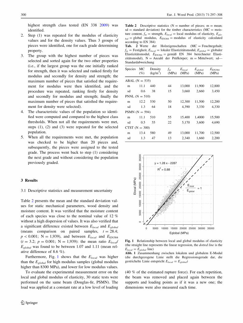
Furthermore, Fig. 1 shows that the Elocal was higher
than the Eglobal for high modulus samples (global modulushigher than 8300 MPa), and lower for low modulus values.
To evaluate the experimental measurement error on the
local and global modulus of elasticity, 30 static tests wereperformed on the same beam (Douglas-fir, PSMN). The
load was applied at a constant rate at a low level of loading
(40 % of the estimated rupture force). For each repetition,the beam was removed and placed again between the
supports and loading points as if it was a new one; the
dimensions were also measured each time.
Table 2 Descriptive statistics (N = number of pieces; m = mean;sd = standard deviation) for the timber characteristics (MC = mois-ture content, fm = strength, Elocal = local modulus of elasticity, Eglo-
bal = global modulus, EEN384 = modulus of elasticity calculatedaccording to EN 384)Tab. 2 Werte der Holzeigenschaften (MC = Feuchtegehalt;fm = Festigkeit, Elocal = lokaler Elastizitatsmodul, Eglobal = globalerElastizitatsmodul, EEN384 = gemaß EN 384 berechneter Elasti-zitatsmodul), N = Anzahl der Prufkorper; m = Mittelwert; sd—Standardabweichung
Species MC(%)
Density(kg/m3)
fm(MPa)
Elocal
(MPa)Eglobal
(MPa)EEN384
(MPa)
ABAL (N = 535)
m 11.1 440 44 13,000 11,900 12,800
sd 0.6 38 15 3,660 2,660 3,450
PNNL (N = 510)
m 12.2 530 50 12,300 11,500 12,200
sd 1.3 64 18 4,390 3,330 4,330
PSMN (N = 594)
m 11.1 510 55 15,400 1,4000 15,500
sd 0.5 55 22 5,170 3,600 4,690
CTST (N = 300)
m 13.4 580 49 13,000 11,700 12,500
sd 1.3 47 13 2,340 1,660 2,200
0 5000 10000 15000 20000 25000 30000 35000
050
0010
000
1500
020
000
2500
030
000
3500
0
Eglobal (MPa)
Elo
cal (
MP
a)
E local
Eglobal
______ = 1
y = 1.28 x - 2287
R2 = 0.88
Fig. 1 Relationship between local and global modulus of elasticity(the straight line represents the linear regression, the dotted line is theElocal = Eglobal line)Abb. 1 Zusammenhang zwischen lokalem und globalem E-Modul(die durchgezogene Linie stellt die Regressionsgerade dar, diegestrichelte Linie entspricht Elocal = Eglobal)
300 Eur. J. Wood Prod. (2013) 71:297–308
123
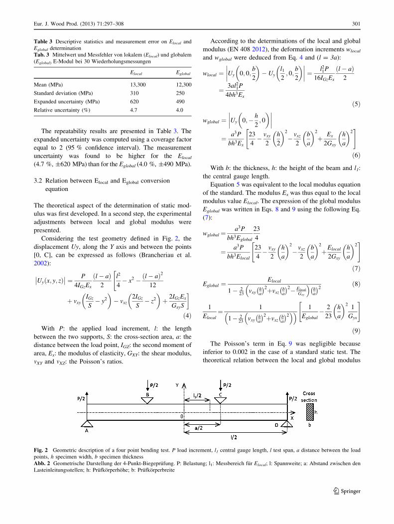
The repeatability results are presented in Table 3. The
expanded uncertainty was computed using a coverage factor
equal to 2 (95 % confidence interval). The measurementuncertainty was found to be higher for the Elocal
(4.7 %, ±620 MPa) than for the Eglobal (4.0 %, ±490 MPa).
3.2 Relation between Elocal and Eglobal conversion
equation
The theoretical aspect of the determination of static mod-
ulus was first developed. In a second step, the experimental
adjustments between local and global modulus werepresented.
Considering the test geometry defined in Fig. 2, the
displacement Uy, along the Y axis and between the points[0, C], can be expressed as follows (Brancheriau et al.
2002):
Uy x; y; z# $'' '' " P
4IGzEx
l% a# $2
l2
4% x2 % l% a# $2
12
"
& vxyIGzS
% y2! "
% vxz2IGzS
% z2! "
& 2IGzEx
GxyS
&
#4$
With P: the applied load increment, l: the length
between the two supports, S: the cross-section area, a: thedistance between the load point, IGZ: the second moment of
area, Ex: the modulus of elasticity, GXY: the shear modulus,
mXY and mXZ: the Poisson’s ratios.
According to the determinations of the local and global
modulus (EN 408 2012), the deformation increments wlocal
and wglobal were deduced from Eq. 4 and (l = 3a):
wlocal " Uy 0; 0;b
2
! "% Uy
l12; 0;
b
2
! "''''
'''' "l21P
16IGzEx
l% a# $2
" 3al21P
4bh3Ex
#5$
wglobal " Uy 0;% h
2; 0
! "''''
''''
" a3P
bh3Ex
23
4% vxy
2
h
2
! "2
% vxz2
b
a
! "2
& Ex
2Gxy
h
a
! "2" #
#6$
With b: the thickness, h: the height of the beam and l1:the central gauge length.
Equation 5 was equivalent to the local modulus equation
of the standard. The modulus Ex was thus equal to the local
modulus value Elocal. The expression of the global modulusEglobal was written in Eqs. 8 and 9 using the following Eq.
(7):
wglobal "a3P
bh3Eglobal
23
4
" a3P
bh3Elocal
23
4% vxy
2
h
a
! "2
%vxz2
b
a
! "2
&Elocal
2Gxy
h
a
! "2" #
#7$
Eglobal "Elocal
1% 223 vxy h
a
( )2&vxz ba
( )2% ElocalGxy
# $ha
( )2 #8$
1
Elocal" 1
1% 223 vxy h
a
( )2&vxz ba
( )2# $# $ 1
Eglobal% 2
23
h
a
! "2 1
Gyx
" #
#9$
The Poisson’s term in Eq. 9 was negligible becauseinferior to 0.002 in the case of a standard static test. The
theoretical relation between the local and global modulus
Table 3 Descriptive statistics and measurement error on Elocal andEglobal determinationTab. 3 Mittelwert und Messfehler von lokalem (Elocal) und globalem(Eglobal) E-Modul bei 30 Wiederholungsmessungen
Elocal Eglobal
Mean (MPa) 13,300 12,300
Standard deviation (MPa) 310 250
Expanded uncertainty (MPa) 620 490
Relative uncertainty (%) 4.7 4.0
Fig. 2 Geometric description of a four point bending test. P load increment, l1 central gauge length, l test span, a distance between the loadpoints, h specimen width, b specimen thicknessAbb. 2 Geometrische Darstellung der 4-Punkt-Biegeprufung. P: Belastung; l1: Messbereich fur Elocal; l: Spannweite; a: Abstand zwischen denLasteinleitungsstellen; h: Prufkorperhohe; b: Prufkorperbreite
Eur. J. Wood Prod. (2013) 71:297–308 301
123
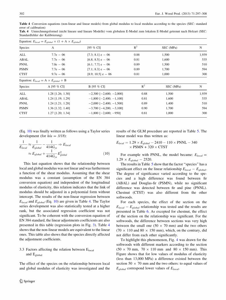
(Eq. 10) was finally written as follows using a Taylor series
development (for h/a = 3/18):
1
Elocal' 1
Eglobal% 1
414Gyx) Elocal
' Eglobal &1
414GyxE2global #10$
This last equation shows that the relationship between
local and global modulus was not linear andwas furthermore
a function of the shear modulus. Assuming that the shearmodulus was a constant (assumption of the EN 384
conversion equation) and independent of the longitudinal
modulus of elasticity, this relation indicates that the link ofmodulus should be adjusted in a polynomial form without
intercept. The results of the non-linear regression between
Elocal and Eglobal (Eq. 10) are given in Table 4. The Taylorseries development was also statistically tested at a higher
rank, but the associated regression coefficient was not
significant. To be coherent with the conversion equation ofEN 384 standard, the linear adjustments coefficients are also
presented in this table (regression plots in Fig. 3). Table 4
shows that the non-linear models are equivalent to the linearones. This table also shows that the species directly affected
the adjustment coefficients.
3.3 Factors affecting the relation between Elocal
and Eglobal
The effect of the species on the relationship between local
and global modulus of elasticity was investigated and the
results of the GLM procedure are reported in Table 5. The
linear model was thus written as:
Elocal " 1:29( Eglobal % 2410% 110( PNNL% 340( PSMN + 320( CTST
For example with PNNL, the model became: Elocal =1.29 9 Eglobal - 2520.
The results in Table 5 show that the factor ‘‘species’’ has a
significant effect on the linear relationship Elocal - Eglobal.The degree of significance varied according to the spe-
cies and a high difference was found between fir
(ABAL) and Douglas-fir (PSMN), while no significantdifference was detected between fir and pine (PNNL).
Chestnut (CTST) was also different from the other
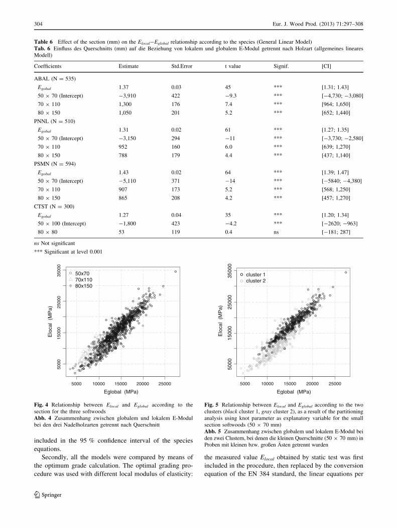
softwoods.For each species, the effect of the section on the
Elocal - Eglobal relationship was tested and the results are
presented in Table 6. As excepted for chestnut, the effectof the section on the relationship was significant. For the
softwoods, the difference between sections was very high
between the small one (50 9 70 mm) and the two others(70 9 110 and 80 9 150 mm), which, on the contrary, did
not differ from each other significantly.
To highlight this phenomenon, Fig. 4 was drawn for thesoftwoods with different markers according to the section
(50 9 70 mm, 70 9 110 mm and 80 9 150 mm). This
Figure shows that for low values of modulus of elasticity(less than 13,000 MPa) a difference existed between the
section 50 9 70 mm and the two others: to equal values of
Eglobal correspond lower values of Elocal.
Table 4 Conversion equations (non-linear and linear models) from global modulus to local modulus according to the species (SEC: standarderror of calibration)Tab. 4 Umrechnungsformel (nicht lineare und lineare Modelle) vom globalem E-Modul zum lokalem E-Modul getrennt nach Holzart (SEC:Standardfehler der Kalibrierung)
Equation: Elocal = Eglobal 9 (1 ? A 9 Eglobal)
Species A [95 % CI] R2 SEC (MPa) N
ALL 7.7e - 06 [7.3; 8.1] e - 06 0.88 1,500 1,939
ABAL 7.7e - 06 [6.8; 8.5] e - 06 0.81 1,600 535
PNNL 7.0e - 06 [6.1; 7.7] e - 06 0.89 1,500 510
PSMN 7.7e - 06 [7.1; 8.3] e - 06 0.89 1,700 594
CTST 9.7e - 06 [8.9; 10.5] e - 06 0.81 1,000 300
Equation: Elocal = A 9 Eglobal ? B
Species A [95 % CI] B [95 % CI] R2 SEC (MPa) N
ALL 1.28 [1.26; 1.30] -2,300 [-2,600; -2,000] 0.88 1,500 1,939
ABAL 1.24 [1.19; 1.29] -1,800 [-2,400; -1,100] 0.81 1,600 535
PNNL 1.24 [1.21; 1.28] -2,000 [-2,400; -1,500] 0.89 1,400 510
PSMN 1.36 [1.32; 1.40] -3,700 [-4,200; -3,100] 0.90 1,700 594
CTST 1.27 [1.20; 1.34] -1,800 [-2,600; -950] 0.81 1,000 300
302 Eur. J. Wood Prod. (2013) 71:297–308
123
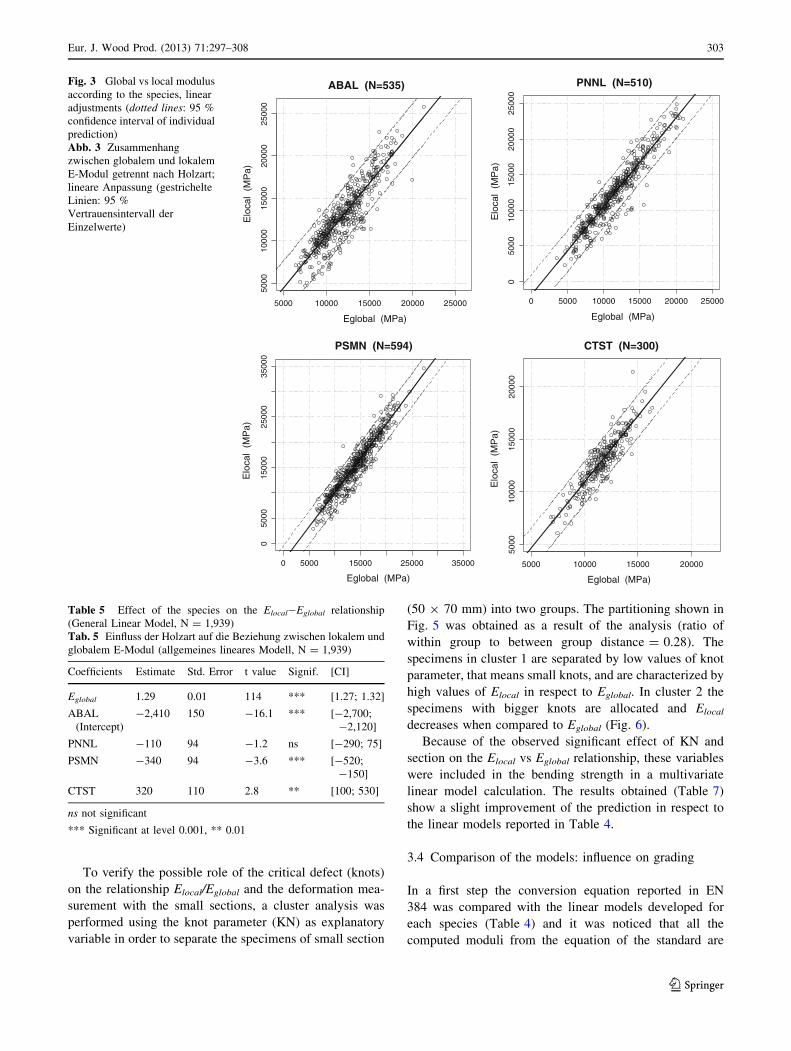
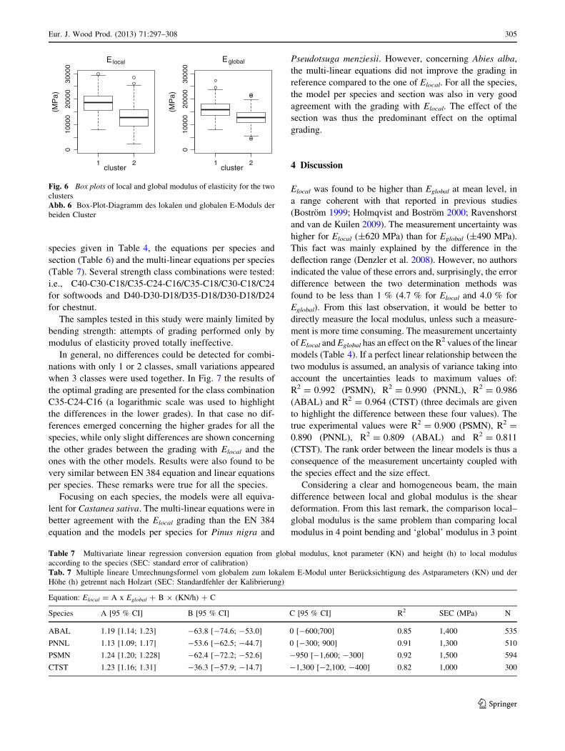
To verify the possible role of the critical defect (knots)
on the relationship Elocal/Eglobal and the deformation mea-surement with the small sections, a cluster analysis was
performed using the knot parameter (KN) as explanatory
variable in order to separate the specimens of small section
(50 9 70 mm) into two groups. The partitioning shown inFig. 5 was obtained as a result of the analysis (ratio of
within group to between group distance = 0.28). The
specimens in cluster 1 are separated by low values of knotparameter, that means small knots, and are characterized by
high values of Elocal in respect to Eglobal. In cluster 2 the
specimens with bigger knots are allocated and Elocal
decreases when compared to Eglobal (Fig. 6).
Because of the observed significant effect of KN andsection on the Elocal vs Eglobal relationship, these variables
were included in the bending strength in a multivariate
linear model calculation. The results obtained (Table 7)show a slight improvement of the prediction in respect to
the linear models reported in Table 4.
3.4 Comparison of the models: influence on grading
In a first step the conversion equation reported in EN384 was compared with the linear models developed for
each species (Table 4) and it was noticed that all the
computed moduli from the equation of the standard are
5000 10000 15000 20000 25000
5000
1000
015
000
2000
025
000
Eglobal (MPa)
Elo
cal
(MP
a)
ABAL (N=535)
0 5000 10000 15000 20000 25000
050
0010
000
1500
020
000
2500
0
Eglobal (MPa)
Elo
cal
(MP
a)
PNNL (N=510)
0 5000 15000 25000 35000
050
0015
000
2500
035
000
Eglobal (MPa)
Elo
cal
(MP
a)
PSMN (N=594)
5000 10000 15000 20000
5000
1000
015
000
2000
0
Eglobal (MPa)
Elo
cal
(MP
a)
CTST (N=300)
Fig. 3 Global vs local modulusaccording to the species, linearadjustments (dotted lines: 95 %confidence interval of individualprediction)Abb. 3 Zusammenhangzwischen globalem und lokalemE-Modul getrennt nach Holzart;lineare Anpassung (gestrichelteLinien: 95 %Vertrauensintervall derEinzelwerte)
Table 5 Effect of the species on the Elocal-Eglobal relationship(General Linear Model, N = 1,939)Tab. 5 Einfluss der Holzart auf die Beziehung zwischen lokalem undglobalem E-Modul (allgemeines lineares Modell, N = 1,939)
Coefficients Estimate Std. Error t value Signif. [CI]
Eglobal 1.29 0.01 114 *** [1.27; 1.32]
ABAL(Intercept)
-2,410 150 -16.1 *** [-2,700;-2,120]
PNNL -110 94 -1.2 ns [-290; 75]
PSMN -340 94 -3.6 *** [-520;-150]
CTST 320 110 2.8 ** [100; 530]
ns not significant
*** Significant at level 0.001, ** 0.01
Eur. J. Wood Prod. (2013) 71:297–308 303
123
included in the 95 % confidence interval of the species
equations.Secondly, all the models were compared by means of
the optimum grade calculation. The optimal grading pro-
cedure was used with different local modulus of elasticity:
the measured value Elocal obtained by static test was first
included in the procedure, then replaced by the conversionequation of the EN 384 standard, the linear equations per
Table 6 Effect of the section (mm) on the Elocal-Eglobal relationship according to the species (General Linear Model)Tab. 6 Einfluss des Querschnitts (mm) auf die Beziehung von lokalem und globalem E-Modul getrennt nach Holzart (allgemeines linearesModell)
Coefficients Estimate Std.Error t value Signif. [CI]
ABAL (N = 535)
Egobal 1.37 0.03 45 *** [1.31; 1.43]
50 9 70 (Intercept) -3,910 422 -9.3 *** [-4,730; -3,080]
70 9 110 1,300 176 7.4 *** [964; 1,650]
80 9 150 1,050 201 5.2 *** [652; 1,440]
PNNL (N = 510)
Egobal 1.31 0.02 61 *** [1.27; 1.35]
50 9 70 (Intercept) -3,150 294 -11 *** [-3,730; -2,580]
70 9 110 952 160 6.0 *** [639; 1,270]
80 9 150 788 179 4.4 *** [437; 1,140]
PSMN (N = 594)
Egobal 1.43 0.02 64 *** [1.39; 1.47]
50 9 70 (Intercept) -5,110 371 -14 *** [-5840; -4,380]
70 9 110 907 173 5.2 *** [568; 1,250]
80 9 150 865 208 4.2 *** [457; 1,270]
CTST (N = 300)
Egobal 1.27 0.04 35 *** [1.20; 1.34]
50 9 100 (Intercept) -1,800 423 -4.2 *** [-2620; -963]
80 9 80 53 119 0.4 ns [-181; 287]
ns Not significant
*** Significant at level 0.001
5000 10000 15000 20000 25000
5000
1500
025
000
3500
0
Eglobal (MPa)
Elo
cal
(MP
a)
°
°
°
°
°°
° °°
°
°°
°
°
°°
°
°°°
°°
°
°
°°
°°°
°°°
°
°°°
°°
°
°°
°
°°
°°°
°°
°°°°°°°
°
°°°
°
°
°
°
°
°
°
° °
°
°°°°
°
°
°
°
°
°
°
°
°
°
°°
°
°
°°
°°
°
°
°
°
°°°°
°° °°
°°°°
°°
°
°°
°°
°
°
°
°°°
°
°°
°
° °°
°°
°
°°
°°
°
°
°°°
°°
°
°
°°
°
°°
°
°°
°°
°°
°
°°°
°°°
°°°
°°
°
°
°°°°
°
°
°°°
°
°°°° °°
°°°
°°
°
°
°
°°
°
°
°
°°
°°
°°
°°°
°°°°
°
°
°°°°
°°
° °°° °
°
°°
°
°
°°
°
°°
° °
°
°
°
°°
°°
°
°
°°
°°
°°°
°
°°°
°
°°
°
°° °
°
°
°°
°
°°
°
° °
°°
°°°°
°
°°
°°
° °
°°
°
°
°°
°
°
°
°°
°
°
°
°°°
°
°°°
°
°
°
° °°
°
° °°
°°
°
°°
°
°
°
°°
°°°°
°
°
°
°°
°
°
°
°°
°°°
°°
°°
°°°
°
°°°
°°°°
°°
°° °°
°
°°
°
°
°°°
°°
°°° °°
°
°
°
°
° °
°°°° °
°
° °
°
°
°°°°
°
°°
°
°°°°°°
°
°
°°
°
°°
°
°
°
°
°
°
°°
°
°°
°
°
°°
°
°°
°
°°
°°
°
°
°°
°
°
°
°
°
°
°
°
°°°
°°
°
°
°° °
°°°°
°
°
°°
° °°
°
°°°
°° °
°°°°°
°
°°
°
°
°
°
°
°°°
°°
°
°
°
°
°
°
°°
° °
°° °
°
°°
°°°
°
°
°
°
° °
°°
°
°
° °°°
°
°
°
°°
°
°°
°° °°°
°
° °
°
°°
°°
°
°°
°°
°
°
°° °
°°°
°
°
°°
°
°° °
°°
°
°
°
°
°
°°
°
°
°°
°
°
°
°
°
°°
°°°
°°°°
°
°
°
°
°°
°°° °
°°
°
°
°
°
° °
°
°° °
°
° °°
°
°
°°
°°
°°
°°
°
°°
°°
°
°
°
°
°
°
°
°
°°
°
°
°
°°
°°
°
°°
°
°
°°°
°°
° °°
°°°
°
°
°
°
°°
° °
°°
°°
°
°
°°°
°
°
°°
° °°°
°°
°°°°
°°°
°
°°
°°
°°°
°
°°
°
°°
°
°
°°°
°°
°° °
°
°
°°
°
°
°°
°°
°°°
°
°
°°°°°° °° °°
°
°°
°°°°°
°°°°
°°
°
°°
°°
°
°
°°
°
°
°°
°°
°°°
° °°
°
°°
°°°°°
°
50x7070x11080x150
Fig. 4 Relationship between Elocal and Eglobal according to thesection for the three softwoodsAbb. 4 Zusammenhang zwischen globalem und lokalem E-Modulbei den drei Nadelholzarten getrennt nach Querschnitt
5000 10000 15000 20000 25000
5000
1500
025
000
3500
0
Eglobal (MPa)
Elo
cal
(MP
a)
°
°°°
°°
°
°°
°°°
°
°°
°°
°
°°
°
°
°
°°°
°°
°°
°°°°
°°°°°°
°
°°
° °
°
°
°
°
° °
°
°
° °°
° °
°
°°
°
°
°°
°
°
°
°
°°°°
°°°
°°
°
°° °
°
°
°
°
° °
°
°
°
°°
°
°
°
°
°
°
°
°
°
°°
°
°°°°°
°°°
°°
°
°°
°
°
°
°
°
°
°
°° °
°
°°°
°
°
°°
°
°
° °°° °°°°
°°
°°
°
°
°°
°
°
°
°
°°
°°
°°°
°°
°°
°°
°
°°°
°
°
°
°
°°
°
° °°
°°
°
°°
°
°
°
°
°
°
°°
°°°° °
°
° °
°
°
°
°
°
°°°
°
°
°
°°°°
°
°
°°
°°
°
°
°
°
°°
°
°
°°
°° °
°
°
°°
° °°
°°
°°
°°°°°
°
°
°
°°
°
°
°°
°
° °
°°
°
°
°
°
°
°
°
°°°
°
°°°
°
°°
°° °°°
°
°°
°
°°
°
°
°
°
°°
°
°
°
°
°°
°
°
°
°°
°°° °
°°
° °°
°
°°
°°° °°
°°
°°
°
°°
°°
°
°
°
°
°°°
°
°°
°°
°°
°
°°
°
° °°
°°°
°°°
°°
°
°°
°°°
°°°
°°°
°°°°
°°
°°
°
°°°°
°°
°
°
°°°
°°°
°
°
°
°°
°°°
°°
°°
° °
°°°°°°°
°
°°
°°°°
° °°
°
°°°
°
°
°
°°
°°
°
°°
°
°
°
° °°
°
°°°
°
°
°°
°
°
°
°
°°°°
°
°°
°°°
°°°°
°
°°
°
° ° °
°°
°°°°
°
°°
°° °
°
°
°°
°°
°
°
°°
°°° °
°°
°
°
°°
°
°
°°°°
°°°
°°
°
°°°°
°°°°°
°
°°
°°
° °°
°°
°°
°°°
°
°°°
°°°
°°
°° °°°°°
°
°°°
°°
°°° °°
°
°
°
°
° °
°
°
°°°°°°°°°°
°
°
°
°
°°
°
°
°
°
° °°
°°
°°
°
°°°
°
°°°°°
°
°
°°
°
°
°°°°°
° °
°
°
°°
°°°
°
°
°°
°°
° °
°
°°°°
°
°
°° °
°°°
°°
°
°
°° °
°°
°°
°°
°
°°
°°
°°°°°
°
°°
°
°° °°° °
°
°
°
°
°°
°
°
°
°
°
°
°
°
°
°°
°°
° °°°°
°
°°
° °
°°
°°°
°
°
°
°°°
°°°
°°°
°°
°
°
°
°° °
°°
°
°
°°°
°°°°°°°°
°°°°°°°
°°
° °°
°
°
°°
°°°
°°°
°
° °°
°°°°
oo
cluster 1cluster 2
Fig. 5 Relationship between Elocal and Eglobal according to the twoclusters (black cluster 1, gray cluster 2), as a result of the partitioninganalysis using knot parameter as explanatory variable for the smallsection softwoods (50 9 70 mm)Abb. 5 Zusammenhang zwischen globalem und lokalem E-Modul beiden zwei Clustern, bei denen die kleinen Querschnitte (50 9 70 mm) inProben mit kleinen bzw. großen Asten getrennt wurden
304 Eur. J. Wood Prod. (2013) 71:297–308
123
species given in Table 4, the equations per species and
section (Table 6) and the multi-linear equations per species(Table 7). Several strength class combinations were tested:
i.e., C40-C30-C18/C35-C24-C16/C35-C18/C30-C18/C24
for softwoods and D40-D30-D18/D35-D18/D30-D18/D24for chestnut.
The samples tested in this study were mainly limited by
bending strength: attempts of grading performed only bymodulus of elasticity proved totally ineffective.
In general, no differences could be detected for combi-nations with only 1 or 2 classes, small variations appeared
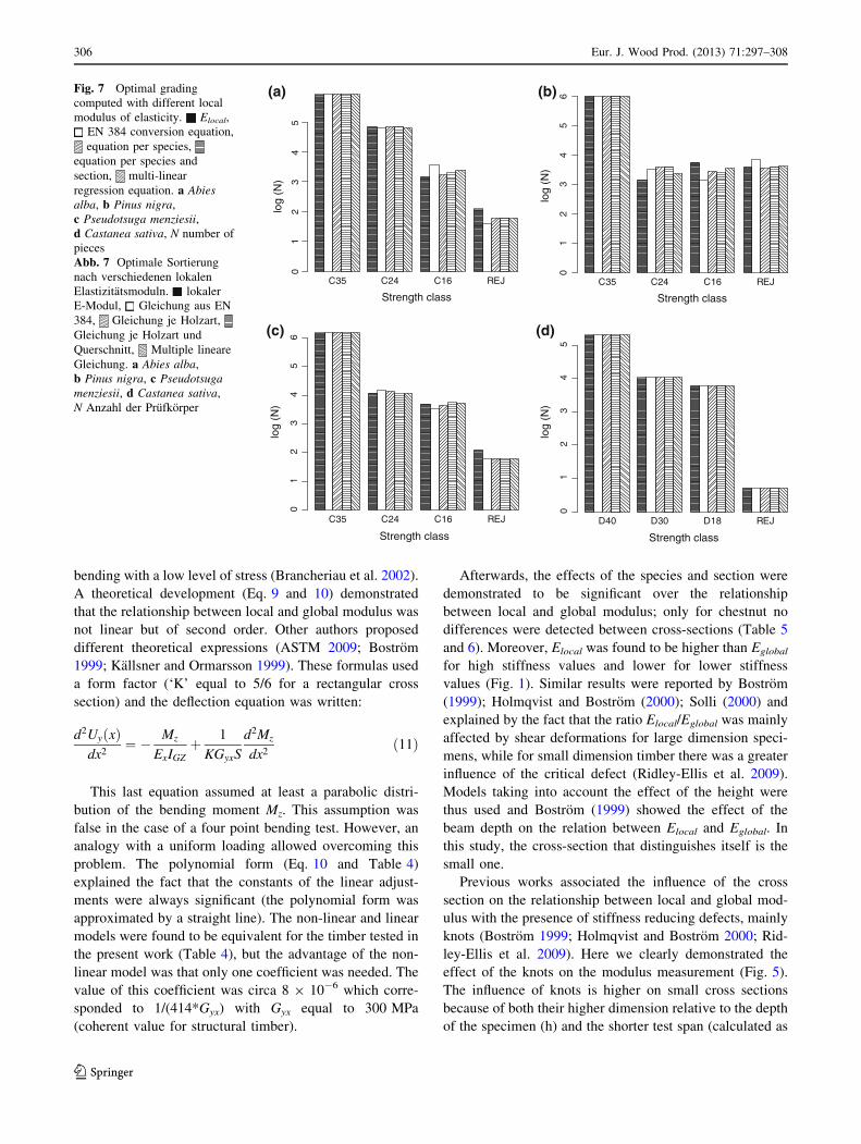
when 3 classes were used together. In Fig. 7 the results of
the optimal grading are presented for the class combinationC35-C24-C16 (a logarithmic scale was used to highlight
the differences in the lower grades). In that case no dif-
ferences emerged concerning the higher grades for all thespecies, while only slight differences are shown concerning
the other grades between the grading with Elocal and the
ones with the other models. Results were also found to bevery similar between EN 384 equation and linear equations
per species. These remarks were true for all the species.
Focusing on each species, the models were all equiva-lent for Castanea sativa. The multi-linear equations were in
better agreement with the Elocal grading than the EN 384
equation and the models per species for Pinus nigra and
Pseudotsuga menziesii. However, concerning Abies alba,the multi-linear equations did not improve the grading inreference compared to the one of Elocal. For all the species,
the model per species and section was also in very good
agreement with the grading with Elocal. The effect of thesection was thus the predominant effect on the optimal
grading.
4 Discussion
Elocal was found to be higher than Eglobal at mean level, in
a range coherent with that reported in previous studies(Bostrom 1999; Holmqvist and Bostrom 2000; Ravenshorst
and van de Kuilen 2009). The measurement uncertainty was
higher for Elocal (±620 MPa) than for Eglobal (±490 MPa).This fact was mainly explained by the difference in the
deflection range (Denzler et al. 2008). However, no authors
indicated the value of these errors and, surprisingly, the errordifference between the two determination methods was
found to be less than 1 % (4.7 % for Elocal and 4.0 % for
Eglobal). From this last observation, it would be better todirectly measure the local modulus, unless such a measure-
ment is more time consuming. The measurement uncertainty
of Elocal and Eglobal has an effect on the R2 values of the linear
models (Table 4). If a perfect linear relationship between the
two modulus is assumed, an analysis of variance taking into
account the uncertainties leads to maximum values of:R2 = 0.992 (PSMN), R2 = 0.990 (PNNL), R2 = 0.986
(ABAL) and R2 = 0.964 (CTST) (three decimals are given
to highlight the difference between these four values). Thetrue experimental values were R2 = 0.900 (PSMN), R2 =
0.890 (PNNL), R2 = 0.809 (ABAL) and R2 = 0.811
(CTST). The rank order between the linear models is thus aconsequence of the measurement uncertainty coupled with
the species effect and the size effect.
Considering a clear and homogeneous beam, the maindifference between local and global modulus is the shear
deformation. From this last remark, the comparison local–
global modulus is the same problem than comparing localmodulus in 4 point bending and ‘global’ modulus in 3 point
1 2
010
000
2000
030
000
E local
cluster
(MP
a)
1 2
010
000
2000
030
000
Eglobal
cluster(M
Pa)
Fig. 6 Box plots of local and global modulus of elasticity for the twoclustersAbb. 6 Box-Plot-Diagramm des lokalen und globalen E-Moduls derbeiden Cluster
Table 7 Multivariate linear regression conversion equation from global modulus, knot parameter (KN) and height (h) to local modulusaccording to the species (SEC: standard error of calibration)Tab. 7 Multiple lineare Umrechnungsformel vom globalem zum lokalem E-Modul unter Berucksichtigung des Astparameters (KN) und derHohe (h) getrennt nach Holzart (SEC: Standardfehler der Kalibrierung)
Equation: Elocal = A x Eglobal ? B 9 (KN/h) ? C
Species A [95 % CI] B [95 % CI] C [95 % CI] R2 SEC (MPa) N
ABAL 1.19 [1.14; 1.23] -63.8 [-74.6; -53.0] 0 [-600;700] 0.85 1,400 535
PNNL 1.13 [1.09; 1.17] -53.6 [-62.5; -44.7] 0 [-300; 900] 0.91 1,300 510
PSMN 1.24 [1.20; 1.228] -62.4 [-72.2; -52.6] -950 [-1,600; -300] 0.92 1,500 594
CTST 1.23 [1.16; 1.31] -36.3 [-57.9; -14.7] -1,300 [-2,100; -400] 0.82 1,000 300
Eur. J. Wood Prod. (2013) 71:297–308 305
123
bending with a low level of stress (Brancheriau et al. 2002).
A theoretical development (Eq. 9 and 10) demonstratedthat the relationship between local and global modulus was
not linear but of second order. Other authors proposed
different theoretical expressions (ASTM 2009; Bostrom1999; Kallsner and Ormarsson 1999). These formulas used
a form factor (‘K’ equal to 5/6 for a rectangular cross
section) and the deflection equation was written:
d2Uy x# $dx2
" % Mz
ExIGZ& 1
KGyxS
d2Mz
dx2#11$
This last equation assumed at least a parabolic distri-
bution of the bending moment Mz. This assumption was
false in the case of a four point bending test. However, ananalogy with a uniform loading allowed overcoming this
problem. The polynomial form (Eq. 10 and Table 4)
explained the fact that the constants of the linear adjust-ments were always significant (the polynomial form was
approximated by a straight line). The non-linear and linear
models were found to be equivalent for the timber tested inthe present work (Table 4), but the advantage of the non-
linear model was that only one coefficient was needed. The
value of this coefficient was circa 8 9 10-6 which corre-sponded to 1/(414*Gyx) with Gyx equal to 300 MPa
(coherent value for structural timber).
Afterwards, the effects of the species and section were
demonstrated to be significant over the relationshipbetween local and global modulus; only for chestnut no
differences were detected between cross-sections (Table 5
and 6). Moreover, Elocal was found to be higher than Eglobal
for high stiffness values and lower for lower stiffness
values (Fig. 1). Similar results were reported by Bostrom
(1999); Holmqvist and Bostrom (2000); Solli (2000) andexplained by the fact that the ratio Elocal/Eglobal was mainly
affected by shear deformations for large dimension speci-
mens, while for small dimension timber there was a greaterinfluence of the critical defect (Ridley-Ellis et al. 2009).
Models taking into account the effect of the height were
thus used and Bostrom (1999) showed the effect of thebeam depth on the relation between Elocal and Eglobal. In
this study, the cross-section that distinguishes itself is the
small one.Previous works associated the influence of the cross
section on the relationship between local and global mod-ulus with the presence of stiffness reducing defects, mainly
knots (Bostrom 1999; Holmqvist and Bostrom 2000; Rid-
ley-Ellis et al. 2009). Here we clearly demonstrated theeffect of the knots on the modulus measurement (Fig. 5).
The influence of knots is higher on small cross sections
because of both their higher dimension relative to the depthof the specimen (h) and the shorter test span (calculated as
(a) (b)
(c) (d)
C35 C24 C16 REJ
Strength class
log
(N)
01
23
45
C35 C24 C16 REJ
Strength class
log
(N)
01
23
45
6
C35 C24 C16 REJ
Strength class
log
(N)
01
23
45
6
D40 D30 D18 REJ
Strength classlo
g (N
)
01
23
45
Fig. 7 Optimal gradingcomputed with different localmodulus of elasticity. Elocal,
EN 384 conversion equation,equation per species,
equation per species andsection, multi-linearregression equation. a Abiesalba, b Pinus nigra,c Pseudotsuga menziesii,d Castanea sativa, N number ofpiecesAbb. 7 Optimale Sortierungnach verschiedenen lokalenElastizitatsmoduln. lokalerE-Modul, Gleichung aus EN384, Gleichung je Holzart,Gleichung je Holzart undQuerschnitt, Multiple lineareGleichung. a Abies alba,b Pinus nigra, c Pseudotsugamenziesii, d Castanea sativa,N Anzahl der Prufkorper
306 Eur. J. Wood Prod. (2013) 71:297–308
123
a function of h). Besides, the stiffness reducing effect is
higher on local than on global modulus because of theposition of knots relative to the reference points for
deflection measurement (closer for local modulus
determination).Finally the comparison of the conversion models was
investigated by means of the optimum grading, such as to
analyse the possible influence of the different conversionfunctions on timber grading. First of all it has to be said
that the study was difficult because the optimum gradingwas strongly dependent on the timber resource (strength
limited timber) and on the grade combination. Several
grade combinations were tested and one combination wasshown, which was able to highlight the differences between
the models (Fig. 7).
Similar results were found between EN 384 equationand linear equations per species. The means were signifi-
cantly different (t test on paired samples): mean differ-
ence = -281 MPa for fir, -121 MPa for pine, 76 MPa forDouglas-fir and -536 MPa for chestnut (Table 2). How-
ever, all the computed moduli from the equation of the
standard were included in the 95 % confidence interval ofthe species equations and the optimum grading procedure
used individual values for grouping the beams by grade.
This remark explained the observed similarity.For softwood, the effect of the section was found to be
the predominant effect on the optimum grading and the
equation per species and section gave similar gradingresults to the Elocal.
A multiple linear model including the amount of defect
in the section and the depth was thus tested. This choicewas motivated because it constituted the simplest type of
multivariate model. However, the efficiency was not better
than a model per species for fir and it was only slightlybetter than the model per species and per section for pine
and Douglas-fir.
The relationship between the local modulus and theseparameters was probably not linear and a specific study
should be done to determine the best non-linear model.
For chestnut, no predominant effect could be identifiedand all the models were comparable. This could be
explained either by the similarity of the cross-sections
tested (80 9 80 mm and 50 9 100 mm), or by a lessinfluence of the defects (knots) on the modulus of elasticity
determination in hardwoods. Therefore, further studies are
needed before a conclusion on that can be drawn.In the end, the conversion equation in the current
European standard (EN 384 2010) can be improved but, in
practice, the conversion equation used can have animportant effect mainly for stiffness limited material: the
optimum grading is dependent on the resource and on the
grade combination. The EN 338 (2009) standard definesthresholds for the characteristic values of density, modulus
of elasticity and bending strength. These thresholds are
ordered from the class the less resistant to the strongestclass. In the two-dimensional space generated by the
modulus of elasticity and the bending strength, the
thresholds are a curve that bounds the resources strength-limited and stiffness-limited. Populations with the modu-
lus-strength point lying below this curve are limited in
strength. The parameter determining the grading is thus thebending strength because for a nearby bending strength of
the threshold value, the average modulus is always greaterthan the standard threshold value. In this particular case,
the bias induced by a conversion equation will have little
influence on the final grading. On the contrary, when themodulus- strength point lies above the curve, the popula-
tions are stiffness-limited. As grading algorithms seek to
approach more closely the boundaries of class, a bias in theconversion equation will have a significant effect on the
final result for the stiffness-limited populations.
The bias of the conversion equation is the uncertainty(confidence interval) induced by the statistical fit between
the local and the global modulus. If this uncertainty is low,
it will be possible to divide the resource in several groups(classes) with a low probability of recovery; that means
quasi-equality between grading from the local modulus and
grading from the conversion equation. The number ofclasses will decrease when uncertainty increases to keep
this quasi-equality between local modulus and conversion
equation. The maximum difference between optimumgrading with the EN 384 equation and with a direct
determination of the local modulus would be reached in the
case of a combination of many grades (3 or more, not verycommon in practice) applied on a stiffness limited resource
(when the modulus of elasticity is the main grading
parameter). However, no difference would be found in thecase of one grade applied to a strength limited resource (in
this case, the main parameter is the modulus of rupture).
Moreover, the EN 384 equation as well as the use oflinear models may lead to higher estimation errors for low
stiffness material (Bogensperger et al. 2006) and, therefore,
to bigger consequences for timber grading. Thus, theconversion equation should be in better agreement with the
theory: Eq. 10 with or without the development in Taylor
series or an equivalent proposed for example by Bogen-sperger et al. (2006). Further analysis could be very
interesting in this direction.
5 Conclusion
Determination of local and global modulus was performed
on 1,939 structural beams of four species with different
cross-sections. The mean value of the local modulus washigher than the global modulus in a ratio of 8.6 %.
Eur. J. Wood Prod. (2013) 71:297–308 307
123
However, the difference was not constant: the local mod-
ulus was superior to the global modulus for the highmodulus samples, and inferior for low modulus values.
The measurement uncertainty was ± 620 MPa for the
local modulus and ± 490 MPa for the global modulus.Nevertheless, the error difference between the two deter-
mination methods was found to be less than 1 %, so as to
reconsider the possibility to directly measure the localmodulus.
A theoretical analysis showed that the relationshipbetween local and global modulus was not linear. This
analysis also indicated that the link of modulus should be
adjusted in a polynomial form with only one coefficient.The factor ‘‘species’’ was found to be significant for the
linear relationship between local and global modulus and
the degree of significance varied according to the species;while the effect of the section was highly significant for the
softwoods, but not for chestnut. The section effect was
explained by the presence and the size of defects in the midspan (knots).
In order to analyse the effect of the different conversion
equations, the local modulus (true values, EN 384 equation,equations per species, equations per species and per sec-
tion, and multi-linear equations per species) were com-
pared by means of the optimum grade calculation. No bigdifferences in the grading results emerged due to the use of
the various models for the timber tested in this work
(strength limited), but dissimilarities could be expectedwhen low stiffness material is analysed.
Acknowledgments The authors thank the Autonomous Province ofTrento (Italy) for funding the mechanical tests; Luciano Scaletti andPaolo Pestelli for the laboratory work.
References
ASTM D198 (2009) Standard test methods of static tests of lumber instructural sizes. ASTM International, West Conshohocken, USA
Bacher M (2008) Comparison of different machine strength gradingprinciples. In: COST E53 Conference 29th–30th October, Delft,The Netherlands, pp 183–193
Bogensperger Th, Schickhofer G, Unterwieser H (2006) Themechanical inconsistence in the evaluation of the modulus ofelasticity according to EN384. CIB W18 Meeting 39, Florence,Italy. Paper 39-21-2
Bostrom L (1997) Measurement of modulus of elasticity in bending.CIB W18 Meeting 30, Vancouver, Canada. Paper 30-10-2
Bostrom L (1999) Determination of the modulus of elasticity inbending of structural timber—comparison of two methods. HolzRoh- Werkst 57(2):145–149
Bostrom L, Ormarsson S, Dahlblom O (1996) On determination ofmodulus of elasticity. CIB W18 Meeting 29, Bordeaux, France.Paper 29-10-3
Brancheriau L, Bailleres H, Guitard D (2002) Comparison betweenmodulus of elasticity values calculated using 3 and 4 pointbending tests on wooden samples. Wood Sci Technol 36(5):367–383
Denzler JK, Stapel P, Glos P (2008) Relationship between global andlocal MOE. CIB W18 Meeting 41, St. Andrews, Canada. Paper41-10-3
EN 13556 (2003) Round and sawn timber—nomenclature of timbersused in Europe. CEN European Committee for Standardization,Brussels
EN 14081-2 (2010) Timber structures—strength graded structuraltimber with rectangular cross section. Part 2: Machine grading;additional requirements for initial type testing. CEN EuropeanCommittee for Standardization, Brussels
EN 338 (2009) Structural timber—strength classes. CEN EuropeanCommittee for Standardization, Brussels
EN 384 (2010) Structural timber—determination of characteristicvalues of mechanical properties and density. CEN EuropeanCommittee for Standardization, Brussels
EN 408 (2012) Timber structures—Structural timber and gluedlaminated timber—determination of some physical and mechan-ical properties. CEN European Committee for Standardization,Brussels
Giudiceandrea F (2005) Stress grading lumber by a combination ofvibration stress waves and X-ray scanning. In: 11th InternationalConference on scanning technology and process optimization inthe wood industry (ScanTech 2005), pp 99–108
Hartigan JA, Wong MA (1979) A K-means clustering algorithm.Appl Stat 28:100–108
Holmqvist C, Bostrom L (2000) Determination of the modulus ofelasticity in bending of structural timber—comparison of twomethods. In: Proceedings of the 6th World Conference onTimber Engineering, 31st July–3rd August, Whistler, Canada
Kallsner B, Ormarsson S (1999) Measurement of modulus ofelasticity in bending of structural timber. RILEM symposiumon timber engineering, Stockholm, pp 639–648
Nocetti M, Bacher M, Brunetti M, Crivellaro A, van de Kuilen JW(2010) Machine grading of Italian structural timber: preliminaryresults on different wood species. In: Proceedings of the 11thWorld Conference on Timber Engineering, 20th–24th June, Rivadel Garda, Italy
R Development Core Team (2011) R: a language and environment forstatistical computing. Available: http://www.r-project.org
Ravenshorst GJ, van de Kuilen JW (2009) Relationship betweenlocal, global and dynamic modulus of elasticity for soft- andhardwoods. CIB W18 Meeting 42, Dubendorf, Switzerland.Paper 42-10-1
Ridley-Ellis D, Moore J, Khokhar A (2009) Random acts of elasticity:MoE, G and EN408. In: Wood EDG Conference, 23rd April2009, Bled, Slovenia
Solli KH (1996) Determination of modulus of elasticity in bendingaccording to EN-408. CIB W18 Meeting 29, Bordeaux, France.Paper 29-10-2
Solli KH (2000) Modulus of elasticity—local or global values. In:Proceedings of the 6th World Conference on Timber Engineer-ing, 31st July–3rd August, Whistler, Canada
308 Eur. J. Wood Prod. (2013) 71:297–308
123