BIS Working PapersNo 417

Relationship and Transaction Lending in a Crisis by Patrick Bolton, Xavier Freixas, Leonardo Gambacorta and Paolo Emilio Mistrulli

Monetary and Economic Department

July 2013

JEL classification: E44, G21

Keywords: Relationship Banking, Transaction Banking, Crisis

BIS Working Papers are written by members of the Monetary and Economic Department of the Bank for International Settlements, and from time to time by other economists, and are published by the Bank. The papers are on subjects of topical interest and are technical in character. The views expressed in them are those of their authors and not necessarily the views of the BIS.

This publication is available on the BIS website (www.bis.org).

© Bank for International Settlements 2013. All rights reserved. Brief excerpts may be reproduced or translated provided the source is stated.

ISSN 1020-0959 (print)

ISBN 1682-7678 (online)

Relationship and Transaction Lendingin a Crisis

Patrick Bolton� Xavier Freixasy Leonardo Gambacortaz

Paolo Emilio Mistrullix

June, 3 2013

AbstractWe study how relationship lending and transaction lending vary

over the business cycle. We develop a model in which relationshipbanks gather information on their borrowers, which allows them toprovide loans for pro�table �rms during a crisis. Due to the servicesthey provide, operating costs of relationship-banks are higher thanthose of transaction-banks. In our model, where relationship-bankscompete with transaction-banks, a key result is that relationship-banks charge a higher intermediation spread in normal times, buto¤er continuation-lending at more favorable terms than transactionbanks to pro�table �rms in a crisis. Using detailed credit registerinformation for Italian banks before and after the Lehman Brothers�default, we are able to study how relationship and transaction-banksresponded to the crisis and we test existing theories of relationshipbanking. Our empirical analysis con�rms the basic prediction of themodel that relationship banks charged a higher spread before the cri-sis, o¤ered more favorable continuation-lending terms in response tothe crisis, and su¤ered fewer defaults, thus con�rming the informa-tional advantage of relationship banking.JEL: E44, G21Keywords: Relationship Banking, Transaction Banking, Crisis

�Columbia University, NBER and CEPR.yUniversitat Pompeu Fabra, Barcelona Graduate School of Economics and CEPR.zBank for International Settlements.xBanca d�Italia.

1

1 Introduction1

What is the role of banks in the real economy? Beyond providing loans to�rms and households, commercial banks have long been thought to play alarger role than simply that of screening loan applicants one transaction ata time. By building a relationship with the �rms they lend to, banks canalso play a continuing role of managing �rms��nancial needs as they arise, inresponse to either new investment opportunities or to a crisis. What deter-mines whether a bank and a �rm should seek to build a long-term relation-ship, or whether they should simply seek to engage in a one-o¤ transaction?Or, equivalently, how do relationship loans di¤er from transaction loans? Weaddress these questions from both a theoretical and an empirical perspective.Relationship banking can take many forms. Moreover, in developed �nan-

cial markets �rms have many options available to them and can choose anycombination of cheaper transaction borrowing and more expensive relation-ship banking that best suits their risk characteristics. Obviously, a �rm willonly choose the more expensive relationship-banking option if the servicesit obtains from the relationship bank are su¢ ciently valuable. Accordingly,the question arises of what type of bene�ts the �rm obtains from a bankingrelationship, and how these bene�ts shape the choice between transactionand relationship banking.The �rst models on relationship banking portray the relationship between

the bank and the �rm in terms of an early phase during which the bankacquires information about the borrower, and a later phase during whichit exploits its information monopoly position (Sharpe 1990). While these�rst-generation models provide an analytical framework describing how thelong-term relationship between a bank and a �rm might play out, they do not

1We would like to thank Claudio Borio, Lars Norden, Greg Udell and in particular twoanonymous referees for comments and suggestions. The opinions expressed in this paperare those of the authors only and do not necessarily re�ect those of the Bank of Italy or theBank for International Settlements. Support from 07 Ministerio de Ciencia e Innovación,Generalitat de Catalunya, Barcelona GSE, Ministerio de Economía y Competitividad) -ECO2008-03066, Banco de España-Excelencia en Educación-�Intermediación Financieray Regulación� is gratefully acknowledged. This study was in part developed while PaoloEmilio Mistrulli was ESCB/IO expert in the Financial Research Division at the EuropeanCentral Bank.

2

consider a �rm�s choice between transaction lending and relationship bankingand which types of �rms are likely to prefer one form of borrowing over theother.The second-generation papers on relationship banking that consider this

question and that have been put to the data focus on three di¤erent and in-terconnected roles for a relationship bank (or R�bank for short): insurance,monitoring and screening. The literature emphasizes these last three rolesdi¤erently, with a �rst strand focusing more on the (implicit) insurance roleof R-banks (for future access to credit and future credit terms) (Berger andUdell, 1992; Berlin and Mester 1999); a second strand underscoring more themonitoring role of R�banks (Holmstrom and Tirole 1997, Boot and Thakor2000, Hauswald andMarquez 2000); and a third strand playing up the greaterscreening abilities (of new loan applications) of R-banks due to their accessto both hard and soft information about the �rm (Agarwal and Hauswald2010, Puri et al. 2010).A fourth somewhat distinct role of relationship banks, which we center on

in this paper, is learning about borrower�s type over time. This role is closerto the one emphasized in the original contributions by Rajan(1992) and VonThadden(1995), and puts the R�bank in the position of o¤ering continuationlending terms that are better adapted to the speci�c circumstances in whichthe �rm may �nd itself in the future. The model of relationship-lendingwe develop here builds on Bolton and Freixas (2006), which considers �rms�choice of the optimal mix of �nancing between borrowing from an R�bankand issuing a corporate bond. Most �rms in practice are too small to beable to tap into the corporate bond market, and the choice between issuinga corporate bond or borrowing from a bank is not really relevant to them.However, as we know from Detragiache, Garella and Guiso (2000) and oth-ers,2 these �rms do have a choice between multiple sources of bank lending,and in particular they have a choice between building a banking relationship(by borrowing from an R�bank) or simply seeking a loan on a one-o¤ basisfrom a transaction lender (or T�bank for short). Accordingly, we modify themodel of Bolton and Freixas (2006) to allow for a choice between borrowingfrom an R�bank or a T�bank (or a combination of the two). The other key

2Our model thus also relates to the rich literature on �rms�choice of the number ofbanks they deal with (Houston and James, 1996; Farinha and Santos, 2002; Detragiache,Garella and Guiso, 2000). This literature, typically does not distinguish between M orT�banks and mainly considers the diversi�cation bene�ts of relying on multiple bankfunding sources.

3

modi�cation of the Bolton and Freixas (2006) model is to introduce aggre-gate business-cycle risk, to allow �rms to di¤er in their exposure to this risk,and to consider how the response of R�banks to a crisis di¤ers from that ofT�banks.The main predictions emerging from the theoretical analysis are that

�rms will generally seek a mix of R�banking and T�banking in an e¤ort toreduce their cost of borrowing. Mainly, the �rms relying on R�banking arethe ones that are more exposed to business-cycle risk and that have the riskiercash �ows. These �rms are prepared to pay higher borrowing costs on theirrelationship loans in order to secure better continuation �nancing terms in acrisis. The �rms relying on a banking relationship are better able to weathera crisis and are less likely to default than �rms relying only on transactionlending, even though the underlying cash �ow risk of �rms borrowing froman R�bank is higher than that of �rms relying only on T�banking.As intuitive as these predictions are, they di¤er in important ways from

those of other relationship banking theories. Table 1 summarizes the maindi¤erences in the empirical predictions of the four di¤erent types of mod-els of relationship banking. Our main �nding is that, consistent with ourpredictions and those of ex-ante screening models, R�banks display lowerloan delinquency rates relative to T�bank. However, unlike the predictionsof screening-based models, we also �nd that T�banks raised loan interestrates more than R�banks in crisis times, providing further support for ourlearning hypothesis of relationship lending.Our study is the �rst to consider how relationship lending responds to

a crisis in a comprehensive way both from a theoretical and an empiricalperspective. Similar to Detragiache, Garella and Guiso (2000) we rely ondetailed credit register information on loans granted by Italian banks to Ital-ian �rms. Our sample covers loan contracts between a total of 179 Italianbanks and more than 72.000 �rms during the period 2007-2010, with thecollapse of Lehman Brothers marking the transition to the crisis. The degreeof detail of our data goes far beyond what has been available in previousstudies of relationship banking. For example, one of the most important ex-isting studies by Petersen and Rajan (1994) only has data on �rms�balancesheets and on the characteristics of their loans, without additional speci�cinformation on the banks �rms are borrowing from.3 As a result they cannot

3They have a dummy variable taking the value 1 if the loan was granted by a bank and0 if granted by another �nancial institution, but they do not have information on which

4

control for bank speci�c characteristics. We are able to do so for both bankand �rm characteristics since we observe each bank-�rm relationship. Moreimportantly, by focusing on multiple lender situations we can run estimateswith both bank and �rm �xed e¤ects, thus controlling for observable andunobservable supply and demand factors. We are therefore able to uncoverthe e¤ects of bank-�rm relationship characteristics on lending precisely. Therichness of our data set allows us to estimate our model with and withoutbank and �rm �xed e¤ects. It turns out that our results di¤er signi�cantlydepending on whether we include or exclude these �xed e¤ects, suggestingthat further research may be called for to corroborate Petersen and Rajan�s�ndings as well as those of other similar studies. Also, unlike the vast ma-jority of the studies, our database includes detailed information on interestrates for each loan. This allows us to investigate bank interest rate settingin good and bad times in a direct way, without relying on any assumptions.4

Overall, our study suggests that relationship banking plays an importantrole in dampening the e¤ects of negative shocks following a crisis. The �rmsthat rely on relationship banks are less likely to default on their loans and arebetter able to withstand the crisis thanks to the more favorable continuationlending terms they can get from R�banks. These �ndings suggest that thefocus of Basel III on core capital and the introduction of countercyclicalcapital bu¤ers could enhance the role of R�banks in crises and reduce therisk of a major credit crunch especially for the �rms that choose to rely onR�banks.The paper is structured as follows. In section 2 we describe the theoretical

model of T�banking and R�banking and in section 3 we deal with how �rmscombine the two forms of funding. In section 4 we compare the �rm�s bene�tsfrom pure T�banking with the ones of mixed �nance, and the implication for

bank granted the loan and they do not have balance sheet information on the bank.4In one related paper Gambacorta and Mistrulli (2013) investigate whether bank and

lender-borrower relationship characteristics had an impact on the transmission of theLehman default shock by analysing changes in bank lending rates over the period 2008:Q3-2010:Q1. Bonaccorsi di Patti and Sette (2012) take a similar approach over the period2007:Q2-2008:Q4, while Gobbi and Sette (2012) consider 2008:Q3-2009:Q3. Albertazziand Marchetti (2010) and De Mitri et al. (2010) complement the previous studies byinvestigating the e¤ect of the �nancial crisis on lending growth. In this paper, we focusinstead on the level of lending rates and the quantity of credit (instead than their respec-tive changes). Moreover, we analyse the behaviour of relationship and transactional banksby comparing bank prices and quantities both in �normal�times and in a crisis. Althoughour results are not perfectly comparable, they are consistent with the above cited papers.

5

the capital bu¤ers the banks have to hold. In Section 5 we test the empiricalimplications of the model and section 6 concludes.

2 The model

We consider the �nancing choices of a �rm that may be more or less ex-posed to business-cycle risk. The �rm may borrow from a bank o¤eringrelationship-lending services, an R�bank, or from a bank o¤ering only trans-action services, a T�bank. As we explain in greater detail below, R�bankshave higher intermediation costs than T�banks, �R > �T , because they haveto hold more equity capital against the expectation of more future roll-overlending. We shall assume that the banking sector is competitive, at leastex ante, before a �rm is locked into a relationship with an R�bank. There-fore, in equilibrium each bank just breaks even and makes zero supra-normalpro�ts. We consider in turn, 100% T� bank lending, 100% R�bank lending,and �nally a combination of R and T�bank lending.

2.1 The Firm�s Investment and Financial Options

The �rm�s manager-owners have no cash but have an investment projectthat requires an initial outlay of I = 1 at date t = 0 to be obtained throughexternal funding. If the project is successful at time t = 1, it returns V H . Ifit fails, it is either liquidated, in which case it produces V L at time t = 1,or it is continued in which case the project�s return depends on the �rm�stype, H or L. For the sake of simplicity, we assume that the probability ofsuccess of a �rm is independent of its type. An H��rm�s expected secondperiod cash �ow is V H , while it is zero for an L��rm. The probability that a�rm is successful at time t = 1 is observable, and the proportion of H��rmsis known. Moreover, both the probability of success and the proportion ofH��rms change with the business cycle, which we model simply as twodistinct states of the world: a good state for booms (S = G) and a bad statefor recessions (S = B). Figure 1 illustrates the di¤erent possible returns ofthe project depending on the bank�s decision to liquidate or to roll over theunsuccessful �rm at time t = 1.5

5A model with potentially in�nitely-lived �rms subject to periodic cash-�ow shocksand that distinguishes between the value to the �rm and to society of being identi�ed asan H-type, would be a better representation of actual phenomena. In a simpli�ed way our

6

We denote the �rms�probability of success at t = 1 as pS, with pG > pB �0. We further simplify our model by making the idiosyncratic high (V H) andlow (0) returns of �rms at time t = 2 independent of the business cycle; onlythe population of H��rms, which we denote by �S will be sensitive to thebusiness cycle. Finally, recession states (S = B) occur with probability �and boom states (S = G) occur with the complementary probability (1� �).The prior probability (at time t = 0) that a �rm is of type H is denoted

by �. This probability belief evolves to respectively �B in the recession stateand �G in the boom state at time t = 1, with �B < �G. The conditionalprobability of a �rm being of type H knowing it has defaulted in time t = 1will be denoted by

� � (1� �)(1� pG)�G + �(1� pB)�B(1� p)

:

As in Bolton and Freixas (2006), we assume that the �rm�s type is privateinformation at time t = 0 and that neither R nor T banks are able to identifythe �rm�s type at t = 0. At time t = 1 however, R�banks are able to observethe �rm�s type perfectly by paying a monitoring cost m > 0, while T�bankscontinue to remain ignorant about the �rm�s type (or future prospects).Firms di¤er in the observable probability of success p = �pB + (1� �)pG.

For the sake of simplicity we take pG = pB + � and assume that pG isuniformly distributed on the interval [�; 1], so that pB is U � [0; 1��] andp is U � [(1� �)�; 1� ��]. Note that for every p there is a unique pair(pB; pG) so that all our variables are well de�ned.Firms can choose to �nance their project either through a transaction

bank or through a relationship bank (or a combination of transaction and re-lationship loans). To keep the corporate �nancing side of the model as simpleas possible, we do not allow �rms to issue equity. The main distinguishingfeatures of the two forms of lending are the following:

1. Transaction banking: a transaction loan speci�es a gross repaymentrT (p) at t = 1. If the �rm does not repay, the bank has the right toliquidate the �rm and obtains V L. But the bank can also o¤er to roll

model can be reinterpreted so that the value of � takes already into account this long runimpact on the �rms�reputation. Still, a systematic analysis of intertemporal e¤ects wouldrequire tracking the balance sheets for both the �rm and of two types of banks as statevariables of the respective value functions and would lead to an extremely complex model.

7

over the �rm�s debt against a promise to repay rST (pS) at time t = 2.This promise rST (pS) must, of course, be lower than the �rm�s expectedsecond period pledgeable cash �ow, which is V H for an H��rm andzero for an L��rm. Thus, if the transaction bank�s belief �S that it isdealing with an H��rm is high enough, so that

rST (pS) � �SVH ;

the �rm can continue to period t = 2 even when it is unable to repayits debt rT (p) at t = 1. If the bank chooses not to roll over the �rm�sdebt, it obtains the liquidation value of the �rm�s assets V L at t = 1.

The market for transaction loans at time t = 1 is competitive andsince no bank has an informational advantage on the credit risk of the�rm the roll-over terms rST (pS) are set competitively. Consequently, ifgross interest rates are normalized to 1, competition in the T�bankingindustry implies that

�SrST (pS) = rT (p); (1)

(when the project fails at time t = 1 the �rm has no cash �ow availabletowards repayment of rT (p); it therefore must roll over the entire loanto be able to continue to date t = 2).

For simplicity, we will assume that in the boom state an unsuccessful�rm will always be able to get a loan to roll over its debt rT (p):

rT (p)

�G� V H : (2)

A su¢ cient condition for this inequality to hold is that it is satis�edfor pG = �.6

By the same token, in a recession state �rms with a high probabilityof success will be able to roll over their debt rT (p) if �B is such that

rT (p)

�B� V H ; (3)

This will occur only for values of pB above some threshold p̂B for whichcondition (3) holds with equality, a condition that, under our assump-tions, is equivalent to p � bp; where bp = p̂B + (1� �)�. In other words,

6Note that the condition is not necessary as in equilibrium some �rms with low p maynot be granted credit at time t = 0 anyway.

8

for low probabilities of success p < bp, an unsuccessful �rm at t = 1in the recession state will simply be liquidated, and the bank then re-ceives V L, and for higher probabilities of success, p � bp (or pB � p̂B)an unsuccessful �rm at t = 1 in the recession state will be able to rollover its debt. Figure 2 illustrates the di¤erent contingencies for thecase pB � p̂B.

2. Relationship banking: Under relationship banking the bank incursa monitoring cost m > 0 per unit of debt,7 which allows the bank toidentify the type of the �rm perfectly in period 1. A bank loan in period0 speci�es a repayment rR(p) in period 1 that has to compensate thebank for its higher funding costs �R > �T .

The higher cost of funding is due to the need of holding higher amountsof capital that are required in anticipation of future roll-overs. It canbe shown, by an argument along the lines of Bolton and Freixas (2006),that as the R-banks are �nancing riskier �rms, even if, on average theirinterest rates will cover the losses, they need additional capital. In ad-dition R-banks re�nance H-�rms and they do so by supplying lendingto those �rms that do not receive a roll-over from T�banks. As a con-sequence, they also need more capital because of capital requirementsdue to the expansion of lending to H��rms.If the �rm is unsuccessful at t = 1 the relationship bank will be ableto extend a loan to all the �rms it has identi�ed as H��rms and thendetermines a second period repayment obligation of r1R. As the bankis the only one to know the �rm�s type, there is a bilateral negotiationover the terms r1R between the �rm and the bank. We let the �rm�sbargaining power be (1 � �) so that the outcome of this bargainingprocess is r1R = �V H and the H��rm�s surplus from negotiations is(1� �)V H .

In sum, the basic di¤erence between transaction lending and relationshiplending is that transaction banks have lower funding costs at time t = 0 butat time t = 1 the �rm�s debt may be rolled over at dilutive terms if thetransaction bank�s beliefs that it is facing an H��rm �B are too pessimistic.

7Alternatively, the monitoring cost could be a �xed cost per �rm, and the cost wouldbe imposed on the proportion � of good �rms in equilibrium. This alternative formulationwould not alter our results.

9

Moreover, the riskiest �rms with p < bp will not be able to roll over theirdebts with a transaction bank in the recession state. Relationship bankinginstead o¤ers higher cost loans initially against greater roll-over security butonly for H��rms.

3 Equilibrium Funding

Our set up allow us to determine the structure of funding and interest ratesat time t = 1 and t = 2 under alternative combinations of transaction andrelationship loans. We will consider successively the cases of pure transactionloans, pure relationship loans, and a combination of the two types of loans.We assume for simplicity that the intermediation cost of dealing with a bank,whether T�bank or R�bank is entirely �capitalized�in period 0 and re�ectedin the respective costs of funds, �T and �R:We will assume as in Bolton andFreixas (2000, 2006) thatH��rms move �rst and L��rms second. The latterhave no choice but to imitate H��rms by pooling with them, for otherwisethey would perfectly reveal their type and receive no funding.

Transaction Banking: Suppose that the �rm funds itself entirely throughtransaction loans. Then the following proposition characterizes equilibriuminterest rates and funding under transaction loans.Proposition 1: Under T�banking, �rms characterized by p � bp are

never liquidated and pay an interest rate

rST =1

�S

on their rolled over loans.For �rms with p < bp there is no loan roll-over in recessions, and the

roll-over of debts in booms is granted at the equilibrium repayment promise:

rGT =1

�G:

The equilibrium lending terms in period 0 are then:

rT (p) = 1 + �T for p � bp: (4)

rT (p) =1 + �T � �(1� pB)V

L

�pB + 1� �for p < bp:

10

Proof: See the Appendix. �

Relationship Banking: Consider now the other polar case of exclu-sive lending from an R�bank. The equilibrium interest rates and fundingdynamics are then given in the following proposition.

Proposition 2: Under relationship-banking there is always a debt roll-over for H��rms at equilibrium terms

r1R = �V H :

The equilibrium repayment terms in period 0 are then given by:

rR(p) =1 + �R � (1� p)[(1� �)V L + �(1�m)�V H ]

�pB + (1� �)pG: (5)

Proof: See the Appendix. �Combining T and R�banking: In the previous two cases of either

pure T banking or pure R�banking the structure of lending is independentof the �rm�s type. When we turn to the combination of T and R�banking,the �rms�choice might signal their type. As mentioned this implies that theL��rms will have no choice but to mimick the H��rms.Given that transaction loans are less costly (�T < �R) it makes sense for

a �rm to rely as much as possible on lending by T�banks. However, there isa limit on how much a �rm can borrow from T�banks, if it wants to be ableto rely on the more e¢ cient debt restructuring services of R�banks. Thelimit comes from the existence of a debt overhang problem if the �rms areoverindebt with T�banks.To see this, let LR and LT denote the loans granted by respectively

R�banks and by T�banks at t = 0, with LR+LT = 1. Also, let rRTR and rRTTdenote the corresponding repayment terms under each type of loan. When a�rm has multiple loans an immediate question arises: what is the senioritystructure of these loans? As is common in multiple bank lender situations,we shall assume that R�bank loans and T�bank loans are pari passu in theevent of default. Under this assumption, the following proposition holds:

Proposition 3: The optimal loan structure for H��rms is to maxi-mize the amount of transactional loans subject to satisfying the relationshiplender�s incentive to roll over the loans at t = 1.

11

The �rm borrows:

LT =(p+ (1� p)�)

��V H(1�m)� V L

�1 + �T � V L

: (6)

in the form of a transaction loan, and (1�LT ) from an R-bank at t = 0at the following lending terms:

rRTT =(1 + �T )� (1� p)(1� �)V L

p+ (1� p)�; (7)

and,

rRTR =1

p

�(1 + �R)�

(1� p)V L

(1� LT )

�: (8)

At time t = 1 both transaction and relationship-loans issued by H � �rmsare rolled over by the R-bank. Neither loan issued by an L � �rm is rolledover.

Proof: See the Appendix. �As intuition suggests: i) pure relationship lending is dominated under our

assumptions; and ii) if the bank has access to securitization or other forms offunding to obtain funds on the same terms as T�banks, then it can combinethe two.Note �nally that, as T�loans are less expensive, a relatively safe �rm

(with a high p) may still be better o¤ borrowing only from T�banks andtaking the risk that with a small probability it won�t be restructured inbad times. We turn to the choice of optimal mixed borrowing versus 100%T��nancing in the next section.

4 Optimal funding choice

When would a �rm choose mixed �nancing over 100% T��nancing? Toanswer this question we need to consider the net bene�t to an H��rm fromchoosing a combination of R and T�bank borrowing over 100% T�bankborrowing. We will make the following plausible simplifying assumptions inorder to focus on the most interesting parameter region and limit the numberof di¤erent cases to consider:

12

Assumption A1: Both (�R � �T ) and m are small enough.

Assumption A2: �V H � V L is not too large so that it satis�es:

�V H � V L < min

((1 + �T )[

(1��)�G

+ ��B� 1]

(1� [(1� �)�G + ��B]);�(1� pB)(V

H � V L)

(1� p)(1� �)

)

These two conditions essentially guarantee that relationship banking hasan advantage over transaction banking. For this to be true, it must be thecase that: First, the intermediation cost of relationship banks is not too largerelative to that of transaction banks. Assumption A1 guarantees that this isthe case. Second, the cost of rolling over a loan with the R�bank should notbe too high. This means that the R�bank should have a bounded ex postinformation monopoly power. This is guaranteed by assumption A2.To simplify notation and obtain relatively simple analytical expressions,

we shall also assume that V H > rT (p)�B. The last inequality further implies

that V H > rT (p)�G

; as �G > �B; so that the �rm�s debts will be rolled over bythe T�bank in both boom and bust states of nature. Note that when this isthe case the transaction loan is perfectly safe, so that rT (p) = 1 + �T ; as inequation (4).We denote by ��(p) = �T (p)��RT (p) the di¤erence in expected payo¤s

for anH��rm from choosing 100% T��nancing over choosing a combinationof T and R�loans and establish the following proposition.

Proposition 4: Under assumptions A1 and A2, the equilibrium fundingin the economy will correspond to one of the three following con�gurations:

1. ��(pmin) � ��((1 � �)�) > 0: monitoring costs are excessively highand all �rms prefer 100% transactional banking.

2. ��(pmax) � ��(1���) > 0 and ��(pmin) � ��((1��)�) < 0: Safe�rms choose pure T�banking and riskier �rms choose a combinationof T�banking and R-banking.

3. ��(pmax) � ��(1 � ��) < 0: all �rms choose a combination ofT�banking and R�banking.

13

Proof: See the Appendix. �

We are primarily interested in the second case, where we have coexistenceof 100% T�banking by the safest �rms along with other �rms combiningT�Banking and R�banking. Notice, that under assumptions A1 and A2, itis possible to write

��((1� �)�) = (�R � �T )(1� L�T ) + (1� (1� �)�)��m�V H

�+��(1 + �T ) + (1� (1� �)�)(1� �)(�V H � V L)

�(1 + �T )[(1� �)(1��)

�G+

�

�B] (9)

and

��(1� ��) = (1 + �R)� (�R � �T )L�T � ��

��(1�m)�V H + (1� �)V L

��(1� ��)(1 + �T ) + ���V H

�(1 + �T )[��

�B]: (10)

Under assumption A1 (�R � �T ) and m are small, so that a su¢ cientcondition to obtain ��(1� ��) > 0 is to have �� su¢ ciently close to zero.Indeed, then we have:

��(1� ��) � (�R � �T )(1� L�T ) > 0

To summarize the predictions of our theoretical model on the basis of theparameter constellation corresponding to case 2 are the following:

� R�banks charge higher lending rates at the initial stage.

� The safest �rms will choose to be �nanced through transaction loans.R�banks will specialize in riskier �rms that will combine R�loans withan amount of transaction loans that is su¢ ciently small not to destroythe incentives of the bank to invest in relationship banking.

14

� In the recession state �rms �nanced exclusively by T�banks will eitherbe denied credit or will face higher interest rates to roll over their loansthan R�banks.

� In a crisis, the rate of default on �rms �nanced exclusively throughtransaction loans will be higher than the rate on �rms �nanced byR�banks:

� Finally, the capital bu¤er of an R-bank will have to be higher than theone of a T�bank, which is consistent with R�banks quoting higherinterest rates in normal times.

5 Empirical analysis

We now turn to the empirical investigation of relationship banking over thebusiness cycle. How do relationship banks help their corporate borrowers?As we have argued, the literature can be divided into four di¤erent typesof theories of relationship banking: 1) relationship-banks o¤er implicit inter-est rate and lending insurance to �rms; 2) relationship-banks monitor �rmsand prevent them from engaging in projects that are not creating value; 3)relationship-banks screen �rm types and weed out excessively risky borrow-ers; and 4) relationship-banks learn the �rm�s type as it evolves and o¤erroll-over loan at favorable terms to the most creditworthy �rms in recessions.These four di¤erent categories of relationship-banking theories have dif-

ferent predictions in terms of delinquency rates, cost of credit, and creditavailability over the business cycle (see Table 1). We test these di¤erentpredictions and speci�cally ask whether:1) According to the (implicit) insurance theory, R�banks do not have

better knowledge about �rms�types and therefore delinquency rates are sim-ilar to those experienced by T�banks in crisis times (see panel I in Table 1).Moreover, by this theory �rms that borrow from R�banks pay higher lendingrates in return for more loans in both states of the world (see, respectively,panel II and III in Table 1).2) According to the monitoring theory (in the vein of Holmstrom and

Tirole, 1997), only �rms with low equity capital choose a monitored bankloan from an R�bank, while �rms with su¢ cient cash (or collateral) choose

15

cheaper loans from a T�bank. By this theory adverse selection is a minorissue, and monitoring is simply a way to limit the �rm�s interim moral haz-ard problems. The monitoring theory predicts higher delinquency rates forR�banks than T�banks, as well as higher lending rates given that R�banksbuild relationships mainly with high-risk low-capital �rms.3) According to the ex-ante screening theory, whereby R�banks rely on

both hard and soft information to weed out bad loan applicants, R�bankshave lower default rates in crisis times than T�banks. And also, given theex-post monopoly of information advantage for R�banks, whether R�bankscharge higher lending rates both in good times and in bad times for the loansthey roll over.4) According to the learning theory, R�banks do not know the �rm�s type

initially but learn it over time. This theory predicts that R�banks chargehigher lending rates in good times on the loans they roll over, but in badtimes they lower rates to help their best clients through the crisis. In contrast,T�banks o¤er cheaper loans in good times but roll over fewer loans in badtimes. Also, according to this theory we should observe lower delinquencyrates in bad times for R�banks that roll over their loans (note that thislatter prediction is also consistent with the ex-ante screening theory).

5.1 Methodology and data

To test these predictions, we proceed in two steps. First we analyze how�rms�default probability in bad times is in�uenced by the fact that the loanis granted by an R�bank or a T�bank. Second, we analyze (and compare)lending and bank interest rate setting in good times and bad times.The �rst challenge is to select two dates that represent di¤erent states of

the world, possibly caused by an exogenous shock that hit the economy. Tothis end we investigate bank-�rm relationships prior and after the LehmanBrothers�default (September 2008) the date typically used to evaluate thee¤ects of the global �nancial crisis (Schularick and Taylor, 2011).In particular, we consider the case of Italy that is an excellent laboratory

for three reasons. First, the global �nancial crisis was largely unexpected(exogenous) and had a sizable impact on Italian �rms, especially small andmedium-sized ones that are highly dependent on bank �nancing. AlthoughItalian banks have been a¤ected as well by the �nancial crisis, systemic sta-bility has not been endangered and government intervention has been negligi-ble in comparison to other countries (Panetta et al. 2009). Second, multiple

16

lending is a long-standing characteristic of the bank-�rm relationship in Italy(Foglia et al. 1998, Detragiache et al. 2000). Third, the detailed data avail-able for Italy allow us to test hypothesis of the theoretical model withoutmaking strong assumptions. For example, the availability of data at thebank-�rm level on both quantity and prices allows us to overtake some ofthe identi�cation limits encountered by the bank lending channel literaturein disentangling loan demand from loan supply shifts (Kashyap and Stein,1995; 2000).The visual inspection of lending and bank interest rates dynamics in Fig-

ure 3 helps us to pick up two dates that can be considered good and badtimes. In particular, we select the second quarter of 2007 as good times be-cause lending dynamic reached a peak, while the interest rate spread appliedon credit lines levelled to a minimum value (see the green circles in panel(a) and (b) of Figure 3). We consider a bad time the �rst quarter of 2010characterized by a negative growth of bank lending to �rms and a very highlevel of the intermediation spread (see the red circles in panel (a) and (b) ofFigure 3). The selection of these two dates is remains consistent also by usingalternative indicators such as real GDP and stock market capitalization (seepanel (c) in Figure 3). We have not considered in our analysis the periodfrom 2011 onwards that has been in�uenced by the e¤ects of the Sovereigndebt crisis.The second choice to be made is how to distinguish T�banks fromR�banks.

As we have seen in the theoretical part of the paper relationship lending isa sort of implicit contract that ensures the availability of �nance to the �rmand allows the bank to partake in the returns. The theoretical literatureagrees on the fact that in order to establish long-lasting and close relation-ships banks need to gather information about the �rm (Boot 2000; Bergerand Udell 2006).As measure of relationship banking we consider in the baseline regressions

the informational distance between lenders and borrowers.8 The empiricalliterature has clearly shown that the distance a¤ects the ability of banks togather soft information, i.e. information that is di¢ cult to codify, which is acrucial aspect of lending relationships (see Berger et al. 2005, Agarwal andHauswald 2010). We therefore divide R�banks and T�banks according to

8There is not a clear consensus in the literature on the way relationship characteris-tics are identi�ed. In Appendix C, we have checked the robustness of the results usingalternative measures for relationship lending.

17

the distance between the lending bank headquarters and �rm headquarters,that we interpret as a form of informational distance. Branches of foreignbanks are considered as T�banks.We argue that distance is strictly related to monitoring costs and, in

general, to the ability of banks to gather soft information. In particular, weargue that the distance between banks�and �rms�headquarters is a proxy forthe cost of producing soft information. Indeed, distance a¤ects the ability ofloan o¢ cers, typically in charge of gathering this kind of information,9 to passit through many hierarchical layers within a bank. Stein (2002) shows thatwhen the production of soft information is decentralized, the incentives togather it crucially depends on the ability of the agent to convey informationto the principal.Distance may a¤ect the transmission of information (i.e. the ability of

branch loan o¢ cers to harden soft information) within banks since banks�headquarters may be less able to interpret the information they receive fromdistant branch loan o¢ cers than from close ones. This is in line with Cre-mer, Garicano and Prat (2007) showing that there is a trade-o¤ betweenthe e¢ ciency of communication within organizations and the scope of theiractivity. In other terms, communication is more di¢ cult when headquartersand branches �di¤er�a lot. Di¤erences of this kind are related to distance forthree main reasons. First, the more banks�headquarters are far away fromborrowers the more costly is for headquarters to gather information directlyand, as a consequence, the greater is the information asymmetry betweenheadquarters and branches. This may reasonably imply a high risk of mis-understandings between branches and headquarters. Second, distance mayalso be a proxy for cultural di¤erences, which again may render the transmis-sion of information di¢ cult. Third, communication problems may stem fromdi¤erences between headquarters and loan o¢ cers in terms of their �institu-tional�memory which are more likely to occur in case branch loan o¢ cersand headquarters are located in very di¤erent areas (Berger and Udell 2004).In particular, to take into account of informational distance, we introduce

two dummy variables: R�bank is equal to 1 if �rm k is headquartered in

9Soft information it is gathered through repeated interaction with the borrower andthen it requires proximity. Banks in order to save on transportation costs delegate theproduction of soft information to branch loan o¢ cers since they are those within bankorganizations which are the closest to borrowers. Alternatively, one can consider thegeographical distance between bank branches and �rms�headquarters. However, Degryseand Ongena (2005) �nd that this measure has little relation to informational asymmetries.

18

the same province where bank j has its headquarters; T�bank is equal to1 if R�bank=0. Monitoring costs can be considered as a positive functionof the distance. This means that a bank can act as an R�bank for a �rmheadquartered in the same province and as a T�bank for �rms that are faraway.Regarding credit risk, the challenge we face is to identify risk and to

distinguish it from asymmetric information, so that we need two di¤erentmeasures. Our theoretical framework is here helpful in clarifying the issue.Indeed, ex ante all banks know that some �rms are more risky than otherswithout investing in relationship banking. This is the knowledge T�banksposses that is represented in our model by p, the probability of success and bya Z�score in our empirical analysis. The Z�score constitutes an indicatorof the ex-ante probability of default. These scores can be mapped into fourlevels of risk: 1) safe; 2) solvent; 3) vulnerable; 4) risky. The Z�scoreis inversely related to the probability of �rms� success p analyzed in thetheoretical model which is a proxy for how sensitive �rms are with respectto the business cycle. The model predicts that it exists a critical thresholdfor the probability of success in bad time p̂B such that for any pB > p̂B�rms prefer pure transactional banking and for any pB < p̂B �rms prefer tocombine the maximum of transactional banking and the minimal amount ofrelationship banking. This means that we should investigate the existence ofa minimum bZ�score such that for any Z < bZ �rms prefer pure transactionalbanking and for any Z > bZ �rms prefer to combine the two kinds of bankingrelationship.Measuring asymmetric information and the role of relationship banks in

gathering it is more complex. Indeed, no contemporaneous variable couldre�ect soft information that is private to the �rm and the relationship bank.Consequently it is only ex post that a variable may re�ect the skills of rela-tionship banking in re�nancing the good �rms and liquidating the bad ones.This superior soft information will imply that relationship banking will havea lower rate of defaults. This is why in order to distinguish H��rms fromL��rms we can observe the realization of defaults.The data come from the Credit Register (CR) maintained by the Bank of

Italy and other sources. Table 2 gives some basic information on the datasetafter having dropped outliers (for more information see the data AppendixB).The table is divided horizontally into three panels: i) all �rms, ii)H��rms

(not gone into default after during the �nancial crisis) and iii) L��rms (de-

19

faulted ones). In the rows we divide bank-�rm relationships in: i) pure rela-tionship lending: �rms which have business relationship with R�banks only;ii) mixed banking relationship: �rms which have business relationships withboth R�banks and T�banks; iii) pure transactional lending: �rms whichhave business relationship with T�banks only.Several clear patterns emerge. First, the situations in which �rms have

only relationships with R�banks (10% of the cases) and T�banks (44% ofthe cases) are numerous but the majority of �rms borrow from both kinds ofbanks (46%). Second, the percentage of defaulted �rms that received lendingby T�banks only is relatively high (64% of the total). Third, in the case ofpure R�banking or combined RT �banking �rms bene�t of a lower increaseof the spread in bad time. Fourth, R�banking is associated with a higherlevel of the capital ratio to be used as bu¤er against contingencies in goodtimes. The slack depends upon the business cycle and it is absorbed in badtimes. Interestingly, the size of the average T�bank is four times that of theaverage R�bank (100 vs 25 billions). This is in line with Stein (2002) whopoints out that the internal management problem of very large intermediariesmay induce these banks to rely solely on hard information, in order to alignthe incentives of the local managers with the headquarters.These patterns are broadly in line with the prescription of the theoretical

model. However, these indications are only very preliminary because thebank-lending relationship is in�uenced not only by �rms�type but also byother factors (sector of �rm�s activity, �rm�s age, �rm�s location, bank-speci�ccharacteristics, etc) for which we are not able to control for in the sampledescriptive statistics reported in Table 2.

5.2 Empirical model and results

As a �rst step of the analysis we focus on the relationship between the proba-bility for a �rm k to go into default and the composition of her transactionalvs relationship �nancing. The baseline cross section equation estimates themarginal probability of �rm k to go into default in the 6 quarters that fol-lowed Lehman�s collapse (2008:q3-2010:q1) as a function of the share of loansthat such �rm has borrowed form a T�bank in 2008:q2. In particular, weestimate the following marginal probit model:

MP (Firm k�s default=1 ) = �+ � + �T � sharek + "k (11)

20

where � and � are, respectively, vectors of bank and industry-�xed e¤ectsand T � sharek is the pre-crisis proportion of transactional loans (in value)for �rm k. The results reported in Table 3 indicate that a �rm �nancedvia T�banking has a higher probability to go into default.10 This marginale¤ect increase with the share of T�bank �nancing and reach the maximum ofaround 0.3% when T�sharek is equal to 1. This e¤ect is not only statisticallysigni�cant but also relevant from an economic point of view because theaverage default rate for the whole sample in the period of investigation wasaround 1.0%. This result remains pretty stable by enriching the set of controlswith additional �rm-speci�c characteristics (see panel II in Table 3) or bycalculating the proportion of transactional loans T � sharek not in value butin terms of the number of banks that �nance �rm k (see panel III in Table3).The positive coe¢ cient � is consistent with two possible explanations of

the nature of relationship lending, namely �learning�and �ex-ante screening�(see Table 1): in both cases relationship banks (R�banks) are better ablethan transactional banks (T�banks) in learning �rms type. Therefore, todistinguish between these two cases we need to analyze lending and interestrate settings of R�banks and T�banks in good times and in bad times (seepanel II and III of Table 1).In the second step of the analysis we investigate bank�s loan and price

setting. Our focus on multiple lending is very useful to solve potential iden-

10In principle the reliability of this test may be bias by the possible presence of �ever-greening�, a practice aimed at postponing the reporting of losses in the balance sheet.Albertazzi and Marchetti (2010) �nd some evidence of �evergreening�practices in Italy inthe period 2008:Q3-2009:Q1, although limited to small banks. We think that evergreeningis less of a concern in our case for three reasons.First, evergreening is a process that by nature cannot postpone the reporting of losses

for a too long time. In our paper, we consider the period 2008:Q3-2010:Q1 that is 18months after Lehmann�s default and therefore there is a higher probability that bankshave reported losses.Second, there is no theoretical background to argue that evergreening can explain the

di¤erence we document between T -banks and R-banks. Both kinds of banks may havea similar incentive to postpone the reporting of losses to temporarily in�ate stock pricesand pro�tability.Third, in the case that R-banks have more incentive to evergreen loans the de�nition of

default used in the paper limits the problem. In particular, we consider a �rm as in defaultwhen at least one of the loans extended is reported to the credit register as a defaultedone (�the �ag is up when at least one bank reports the client as bad�). This means thata R-bank cannot e¤ectively postpone the loss simply because a T -banks will report it.

21

ti�cation issue because the availability of data at the bank-�rm level allowus to include in the econometric model both bank and �rm �xed e¤ects. Inparticular, the inclusion of �xed e¤ects allows us to control for all (observableand unobservable) time-invariant bank and borrower characteristics and todetect in a very precise way the e¤ects of bank-�rm relationship on the bankrate and the lending quantity over time.We estimate two cross-sectional equations for the interest rate (rj;k) ap-

plied by bank j on the credit line of �rm k and the logarithm of outstandingloans in real terms (Lj;k) supplied by bank j on total credit lines of �rm k:

rj;k = � + � + T -bankj;k + "j;k (12)

Lj;k = � + �+ �T -bankj;k + "j;k (13)

where � and � are bank-�xed e¤ects and � and � are �rm-�xed e¤ects. HereZ�scores (proxies for the prior probability of success p) are not includedbecause (observable and unobservable) �rm characteristics are captured by�rm-�xed e¤ects. Both equations are estimated over good time (2007:q2)and bad time (2010:q1).

The results are reported in Table 4.11 In line with the prediction of themodel, the coe¢ cients show that T�banks (compared to R�banks) provideloans at a cheaper rate in good time and at a higher rate in bad time (seecolumns I and II). The di¤erence between the two coe¢ cients B� G =:123 � (�:081) = :204��� is statistically signi�cant. As for loan quantities,other things being equal, T�banks always provide on average a lower amountof lending, especially in bad times (see columns III and IV). In this case thedi¤erence �G� �B = �:313�(�:275) = �0:038�� indicates that, other thingsbeing equal, T�banks supply around 4% less loans in bad times, relativelyto good state of the world.

11Following Albertazzi and Marchetti (2010) and Hale and Santos (2009) we clusterstandard errors ("j;k) at the �rm level in those regressions that include bank �xed e¤ects.Vice versa in those regressions that include speci�c �rm �xed e¤ects (but no bank �xede¤ects) we cluster standard errors at the bank group level. In this way we are able tocontrol for the fact that, due to the presence of an internal capital market, probably�nancial conditions of each bank in the group is not independent of one another. For ageneral discussion on di¤erent approaches used to estimating standard errors in �nancepanel data sets, see Petersen (2009).

22

Equations (12) and (13) can be further enriched with interaction termsbetween bank-types and the Z�score in order to analyze if R-banks andT�banks behave di¤erently with respect to borrowers with a di¤erent degreeof risk:

rj;k = �+�+ T �bankj;k+ ZT �bankj;k �Z+�ZR�bankj;k �Z+�X+"j;k(14)

Lj;k = �+�+�T�bankj;k+�ZT�bankj;k �Z+ ZR�bankj;k �Z+�X+"j;k(15)

In the above equations we can include only bank �xed e¤ects because theintroduction of the interaction terms between bank type and the Z�scores(this linear combination is invariant for each �rm) prevent us from including�rm-�xed e¤ects. For this reason we enrich the set of controls by including acomplete set of industry-province dummies (�) and a vectorX with a numberof �rm-speci�c characteristics. In particular X contains:

� a dummy US>GR that takes the value of 1 for those �rms that haveused their credit lines for an amount greater than the value granted bythe bank, and zero elsewhere;

� a dummy that takes the value of 1 if a company is organized to give itsowners limited liability, and zero elsewhere (LTD);

� a dummy that takes the value of 1 for �rms with less than 20 employees(SMALL_FIRM), and zero elsewhere; this dummy aims at controllingfor the fact that small �rms, due to their great opacity, do not issuebonds as larger �rms do;

� the length of the borrower�s credit history (CREDIT HISTORY) mea-sured by the number of years elapsed since the �rst time a borrowerwas reported to the Credit Register. This variable also tells us howmuch information has been shared among lenders through the CreditRegister over time and it is a proxy for �rms�reputation acquisition.

The results are reported in Table 5. Firms that use their credit linesfor an amount greater than the value granted by the bank have to pay ahigher spread that increase in bad times. Repeated interaction with the

23

banking system also has an e¤ect on bank interest rate setting and loansupply. The variable CREDIT_HISTORY, representing the number of yearselapsed since the �rst time a borrower was reported to the Credit Register, isnegatively (positively) correlated with rates applied to credit lines (amountof outstanding loans). Firms organized with the juridical form of an LTDpay a lower spread and need less lending because they can tap funds also onthe equity and the bond markets.The graphical interpretation of the interaction terms between bank-types

and the Z�score is reported in Figure 4. The upper panels (a) and (b)describes the e¤ects on the interest rate, the bottom panels (c) and (d)those on the logarithm of real loans. The graph on the left illustrate thecase of good times, while the second one bad times. In each graph thehorizontal axis report the Z�score, where Z goes from 1 (safe �rm) to 4(risky �rm). Transactional banking (T�banks) is indicated with a dottedline while relationship banking (R�banks) with a solid line.The visual inspection of all graphs shows that both interest rates and

loans quantities are positively correlated with Z�score. The positive corre-lation between risk and bank �nancing depends probably upon the fact thatrisky �rms have a limited access to market �nancing. As expected also theinterest rate increases with �rms�risk.In line with the prescription of the model the cost of credit of transactional

lending is always lower than relationship banking in good times: the dottedline is always below the solid one for all Z�scores (see panel (a) of Figure 4).This pattern is reversed in bad times (panel (b)) when banks with a stronglending relationship (R�banks) o¤er lower rates to risky �rms (those witha Z�score greater than 1). It is interesting to note that in line with the pre-scription of the model, it is always cheaper for safe �rms to use transactionalbanking because they obtain always a lower rate from T�banks.Moreover the two bottom panels of Figure 4 highlight that the roll-over

e¤ects ofR�banks on lending is in place prevalently for risky �rms while safe�rms obtain always a greater level of �nancing from T�banks both in goodand bad times (the dotted line is always above the solid line for Z=1 bothin panel (c) and panel (d)).An important prescription of the theoretical model is that banks need a

capital bu¤er to be used in order to preserve the lending relationship in badtimes. Since equity is costly this implies that banks with regulatory capitalslack will charge higher interest rates in good times. To test this prescriptionwe focus on the e¤ects of bank capital on interest rate and lending. It is worth

24

stressing that the analysis of interest rates applied on credit lines is partic-ularly useful for our purposes for two reasons. First, these loans are highlystandardized among banks and therefore comparing the cost of credit among�rms is not a¤ected by unobservable (to the econometrician) loan-contract-speci�c covenants. Second, overdraft facilities are loans granted neither forsome speci�c purpose, as is the case for mortgages, nor on the basis of aspeci�c transaction, as is the case for advances against trade credit receiv-ables. As a consequence, according to Berger and Udell (1995) the pricing ofthese loans is highly associated with the borrower-lender relationship, thusproviding us with a better tool for testing the role of lending relationships inbank interest rate setting.In particular, we estimate the following equations where we include the

regulatory capital-to-risk weighted assets ratio (CAP , lagged one period tomitigate endogeneity problems), a set of bank-zone dummies (z) and a setof other bank-speci�c controls (Y ).

rj;k = � + z + T � bankj;k + �CAPj +Y + "j;k (16)

Lj;k = �+ z + �T � bankj;k + �CAPj + �Y + "j;k (17)

The vector Y contains in particular the dummy US > GR, described above,and:

� a dummy for mutual banks (MUTUAL), which are subject to a specialregulatory regime (Angelini et al., 1998);

� a dummy equal to 1 if a bank belongs to a group and 0 elsewhere;

� a dummy equal to 1 if a bank has received government assistance and0 elsewhere.

The results reported in Table 6 indicate that banks with larger capitalratios are better able to protect the lending relationship with their clients.Well-capitalized banks have an higher capacity to insulate their credit port-folio from the e¤ects of an economic downturn by granting an higher amountof lending at a lower interest rate. To get a sense of the economic impact ofthe above-mentioned results, during a downturn a bank with a capital ratio5 percentage points greater with respect to another one supplies 5% moreloans at an interest rate 20 basis points lower. This result on the e¤ects of

25

bank capital is in line with the bank lending channel literature which indi-cates that well-capitalized banks are better able to protect their clients inthe case of monetary policy shocks (Kishan and Opiela, 2000; Gambacortaand Mistrulli, 2004).Interestingly, the positive e¤ect of bank capital in protecting the lending

relationship is more important for R�banks that for T�banks. This can betested by replacing �CAP in equation (16) with

vTT � bank � CAP + vRR� bank � CAP

and �CAP in equation (17) with

�TT � bank � CAP + �RR� bank � CAP

In particular, the coe¢ cients vT and vR take the values of -0.054*** (s.e.0.008) and -0.038*** (s.e. 0.010), respectively, and are statistically di¤erent.A similar result is obtained in the lending equation, where �T and �R havethe values of -0.025*** (s.e. 0.005) and -0.006* (s.e. 0.003), respectively,and are statistically di¤erent one from the other. Making a parallel withthe example above, this means that during a downturn a R�bank (T�bank)with a capital ratio 5 percentage points greater with respect to another onesupplies 12% more loans at an interest rate 27 basis points lower (3% and 19basis point for a T�bank).As a �nal step of the empirical evidence we test the theoretical pre-

scription on bank capital endowments (see Section 5). In particular, sinceT�banks have a lower incentive of making additional loans to good �rms indistress we should observe that these banks detain a lower bu¤er of capitalagainst contingencies with respect to R�banks prior to the crisis.In order to test this prediction we have estimated the following cross

sectional equation on our sample of 179 banks:

CAPj = z + �T � sharej +Y + �Z + "j (18)

where the dependent variable CAPj is the regulatory capital-to-risk weightedassets of bank j at 2008:q2, prior to Lehman�s default. The variable T �sharej is the proportion of transactional loans (in value) for bank j, a setof bank-zone dummies (z), a set of bank-speci�c controls (Y ) and a setof bank credit portfolio-speci�c controls (Z). Bank speci�c characteristicsinclude not only bank�s size and the liquidity ratio (liquid assets over total

26

assets) but also the retail ratio between deposits and total bank funding(excluding capital). All explanatory variables are taken at 2008:q1 in orderto mitigate endogeneity problems. The results reported in Table 7 indicatethat, indipendently of the model speci�cation chosen, a pure T�bank thathave a credit portfolio composed excludively of transactional loans (T �sharej = 1) have a capital bu¤er more than 3 percentage points lower than apure R�bank, whose portfolio is composed exclusively of relationship loans(T � sharej = 0).One distinctive feature of our dataset is that, by focusing on multiple

lending, we are allowed to run estimates with both bank and �rm �xed e¤ects,controlling for observable and unobservable supply and demand factors. Inthis way we are able to clearly detect the e¤ects of bank-�rm relationshipcharacteristics on lending, not biased by the omission of some variables thatmay a¤ect credit conditions. To show this we have therefore re-run all themodels without bank and �rm �xed e¤ects. These new set of results, notreported for the sake of brevity but available from the authors upon request,indicates that T�bank coe¢ cients are often di¤erent, and even change theirsign in one third of the cases. In particular, not introducing �xed-e¤ects,T�banks are shown to supply relatively more lending but at higher prices.This is an important aspect of our work because we show that not controllingfor all unobservable bank and �rm characteristics biases the results and inparticular, the bene�ts of relationship lending tends to be overestimated onprices and underestimated on quantities.The bias can be shown by comparing Figure 4 (that gives a graphical

interpretation of the results of the models with �xed e¤ects reported in Table)with Figure 5 that shows the graphical analysis of the same models reportedin Table 5 without �xed e¤ects. In Figure 5 the dotted line for T�banksmove upwards with respect to Figure 4, in other words T�banks supplyrelatively more loans and charge higher interest rates when �xed e¤ects aredropped compared to the case when they are plugged into the equation.Interestingly from our perspective, this last result also supports the way

we identify transactional and relationship banking. Indeed, the sign of thisbias is consistent with the view that R�banks are better able than T�banksat gathering soft information and then better able at discriminating betweengood and bad borrowers. To explain this let�s think about two �rms thathave the same Z�score but one is, in reality, riskier than the other. Ac-cording to our model, R�banks are better able to discriminate between thetwo while T�banks are not. This happens because T�banks use only hard

27

information (incorporated in the Z�scores) while R�banks rely on bothhard and soft information. If this is true then the riskiest �rm would pre-fer to ask T�banks for a loan since these banks are less able to distinguishgood from bad borrowers. As a consequence, the riskiest �rm will in theoryget better price conditions and a larger amount of credit compared to thecase in which T�banks were able to evaluate their risk correctly. However,T�banks are perfectly aware that the bank-�rm matching is not random andin particular that their set of the pool of applicants is, on average, riskierthan R�banks. As a consequence, T�banks will charge higher interest rates,anticipating that they will tend to make more mistakes in their loan restruc-turing choices, compared to R�banks or, in other terms, that they will tendto lend �too much� and this is exactly what we get in Figure 5 where weare not controlling for this endogenous matching. On the contrary, by using�xed e¤ects we get rid of the fact that the bank-�rm matching is not ran-dom since we compare R�banks�and T�banks�behavior keeping constantand homogenous the level of default risk between banks�type. Only in thislast case we are able to compare R�banks with T�banks perfectly since theinterest rate spread between these two types of banks (and their di¤erentlending behavior) only re�ect the di¤erent role they perform in the creditmarket. Thus the interest spread between R�banks and T�banks in goodtimes reported in Figure 4 (using �xed e¤ects) is a unbiased measure of thepremium that �rms pay in order to get a loan restructuring in bad times.

6 Conclusion

We have found that relationship banking is an important mitigating factorof crises. By helping pro�table �rms to retain access to credit in time ofcrisis relationship banks dampen the e¤ects of a credit crunch. However,the role relationship banks can play in a crisis is limited by the amount ofexcess equity capital they are able to hold in anticipation of a crisis. Banksentering the crisis with a larger equity capital cushion are able to performtheir relationship banking role more e¤ectively. These results are consistentwith other empirical �ndings for Italy (see, amongst others, Albertazzi andMarchetti (2010) and Gobbi and Sette (2012)).Our analysis suggests that if more �rms could be induced to seek a long-

term banking relation, and if relationship banks could be induced to hold abigger equity capital bu¤er in anticipation of a crisis, the e¤ects of crises on

28

corporate investment and economic activity would be smaller. However, ag-gressive competition by less well capitalized and lower-cost transaction banksis undermining access to relationship banking. As these banks compete moreaggressively more �rms will switch away from R�banks and take a chancethat they will not be exposed to a crisis. And the more �rms switch thehigher the costs of R�banks. Overall, the �ercer competition by T�bankscontributes to magnifying the amplitude of the business cycle and the pro-cyclical e¤ects of bank capital regulations.

References

[1] Agarwal, S. and Hauswald R. (2010), �Distance and Private Informationin Lending�, Review of Financial Studies, 23, 2757-2788.

[2] Albertazzi, U. and Marchetti D. (2010), �Credit Supply, Flight to Qual-ity and Evergreening: An Analysis of Bank-Firm Relationships afterLehman�, Bank of Italy, Temi di discussione, 756.

[3] Angelini, P., Di Salvo P. and Ferri G. (1998), �Availability and Cost ofCredit for Small Businesses: Customer Relationships and Credit Coop-eratives�, Journal of Banking and Finance, 22, 925-954.

[4] Berger, A.N., Miller N.H., Petersen M.A. , Rajan R.G., Stein J.C.(2005),�Does function follow organizational form? Evidence from the lendingpractices of large and small banks�, Journal of Financial Economics,76(2), 237-269.

[5] Berger, A.N. and Udell G.F. (1992), �Some Evidence on the EmpiricalSigni�cance of Credit Rationing�, Journal of Political Economy, 100(5),1047-1077.

[6] Berger, A.N. and Udell G.F. (1995). �Relationship Lending and Linesof Credit in Small Firm Finance�, Journal of Business, 68, 351�379.

[7] Berger, A.N. and Udell, G.F. (2004), �The Institutional Memory Hy-pothesis and the Procyclicality of Bank Lending Behavior�, Journal ofFinancial Intermediation, 13, 458-495.

29

[8] Berger, A.N. and Udell, G.F. (2006), �A More Complete ConceptualFramework for SME Finance�, Journal of Banking and Finance, 30,2945�2966.

[9] Berlin, M. and Mester, L. (1999), �Deposits and Relationship Lending�,Review of Financial Studies, 12(3), 579-607.

[10] Bolton, P. and X. Freixas (2000), �Equity, Bonds and Bank Debt: Cap-ital Structure and Financial Market Equilibrium under Asymmetric In-formation�, Journal of Political Economy, 108, 324�351.

[11] Bolton, P. and Freixas X. (2006), �Corporate Finance and the MonetaryTransmission Mechanism�, Review of Financial Studies, 3, 829�870.

[12] Bonaccorsi di Patti, E. and Sette, E. (2012), �Bank Balance Sheets andthe Transmission of Financial Shocks to Borrowers: Evidence from the2007-2008 Crisis�, Bank of Italy, Temi di discussione, 848.

[13] Boot, A.W.A. (2000), �Relationship banking: What do we know?�,Journal of Financial Intermediation, 9, 7-25.

[14] Boot, A. and A. Thakor, (2000), �Can Relationship Banking SurviveCompetition?,�Journal of Finance, American Finance Association, vol.55(2), 679-713, 04.

[15] Cremer, J., Garicano L., and Prat A. (2007), �Language and the Theoryof the Firm�, Quarterly Journal of Economics, 1, 373-407.

[16] De Mitri, S., Gobbi G. and Sette E. (2010), �Relationship Lending in aFinancial Turmoil,�Bank of Italy, Temi di discussione, 772.

[17] Degryse, H. and Ongena S. (2005), �Distance, Lending Relationships,and Competition,�Journal of Finance, 60(1), 231-266.

[18] Detragiache, E., Garella, P. and Guiso, L. (2000), �Multiple versus Sin-gle Banking Relationships: Theory and Evidence�, Journal of Finance,55, 1133-1161.

[19] Farinha, L.A. and Santos J.A.C. (2002), �Switching from Single toMultiple Bank Lending Relationships: Determinants and Implications�,Journal of Financial Intermediation, 11(2), 124�151.

30

[20] Foglia, A., Laviola, S. and Marullo Reedtz, P. (1998), �Multiple Bank-ing Relationships and the Fragility of Corporate Borrowers�, Journal ofBanking and Finance, 22, 1441-1456.

[21] Gambacorta, L. and Mistrulli P. (2004), �Does Bank Capital A¤ectLending Behavior?�, Journal of Financial Intermediation, 13, 436�457.

[22] Gambacorta, L. and Mistrulli P. (2013), �Bank Heterogeneity and Inter-est Rate Setting: What Lessons have we Learned since Lehman Broth-ers?�, Journal of Money Credit and Banking, forthcoming.

[23] Gobbi, G. and Sette E. (2012), �Relationship Lending in a FinancialTurmoil�, Bank of Italy, mimeo.

[24] Hale, G. and Santos, J.A.C. (2009), �Do banks price their informationalmonopoly?�, Journal of Financial Economics, 93, 185-206.

[25] Hauswald, R. and R. Marquez (2000), �Relationship Banking, LoanSpecialization and Competition�, Proceedings, Federal Reserve Bank ofChicago, May, 108-131.

[26] Holmstrom, B. and Tirole J. (1997), �Financial Intermediation, Loan-able Funds and the Real Sector�, Quarterly Journal of Economics,112(3), 663�691.

[27] Houston, J. and James C. (1996), �Bank Information Monopolies andthe Mix of Private and Public Debt Claims�, The Journal of Finance,51(5), 1863�1889.

[28] Kashyap, A. and Stein J.C. (1995), �The Impact of Monetary Policy onBank Balance Sheets�, Carnegie Rochester Conference Series on PublicPolicy, 42, 151-195.

[29] Kashyap, A. and Stein J.C. (2000), �What Do a Million Observationson Banks Say About the Transmission of Monetary Policy�, AmericanEconomic Review, 90, 407-428.

[30] Kishan, R.P. and Opiela T.P. (2000), �Bank Size, Bank Capital and theBank Lending Channel�, Journal of Money, Credit and Banking, 32,121�141.

31

[31] Panetta, F., Angelini P. (coordinators), Albertazzi, U., Columba, F.,Cornacchia, W., Di Cesare, A., Pilati, A., Salleo, C., Santini, G., (2009),�Financial sector pro-cyclicality: lessons from the crisis�, Bank of ItalyOccasional Papers Series, 44.

[32] Petersen, M.A. (2009), �Estimating Standard Errors in Finance PanelData Sets: Comparing Approaches�, Review of Financial Studies, 22,435�480.

[33] Petersen, M. and Rajan R. (1994), �The Bene�ts of Lending Relation-ships: Evidence from Small Business Data�, The Journal of Finance,49, 3�37.

[34] Puri, M., Rocholl J. and Sascha S. (2010) �On the Impor-tance of Prior Relationships in Bank Loans to Retail Cus-tomers�; mimeo, SSRN: http://ssrn.com/abstract=1572673 orhttp://dx.doi.org/10.2139/ssrn.1572673

[35] Rajan, R. (1992), �Insiders and Outsiders: The Choice Between In-formed Investors and Arm�s Lenght Debt�, Journal of Finance, 47(4),1367�1400.

[36] Schularick, M. and Taylor A.M. (2011), �Credit booms gone bust: mon-etary policy, leverage and �nancial crises, 1870-2008�, American Eco-nomic Review, forthcoming.

[37] Sharpe, S.A. (1990), �Asymmetric Information, Bank Lending and Im-plicit Contracts: A Stylized Model of Customer Relationships�, Journalof Finance, 45(4), 1069�1087.

[38] Stein, J.C. (2002), �Information Production and Capital Allocation: De-centralized Versus Hierarchical Firms�, Journal of Finance, 57, 1891-1921.

[39] Von Thadden, E. L. (1995), �Long-term contracts, short-term invest-ment and monitoring�, Review of Economic Studies, 62, 557�575.

32

Appendix A. Mathematical proofs

Proof of Proposition 1We shall characterize the equilibrium lending terms and loan re�nancing

using backwards induction. These lending terms and roll-over decisions willdepend on whether we are considering a safe �rm for which condition (3)holds (p � bp) or a risky �rm (p < bp).� If the project is successful, �rms are able to repay their loan out oftheir cash �ow V H . This occurs with probability pS. In this case the�rm continues to period 2 and gets V H if it is an H��rm.

� If the project fails at time t = 1, �rms with p � bp will be able to rollover their debts. Their debt will then be rolled over against a promisedrepayment of rST (pS) that re�ects state of nature S. When with p � bp,H��rms are able to make su¢ ciently high promised expected repay-ments �BrBT (pB) even in the recession state, so that for these �rms wehave rT (p) given by the break-even condition:

rT (p) = 1 + �T :

� If, instead p < bp, liquidation occurs in state B if the �rm is not suc-cessful, which happens with probability �(1 � pB). The gross interestrate rT (p) is then given by the break even condition:

[p+ (1� �)(1� pG)] rT (p) + �(1� pB)VL = 1 + �T :

Proof of Proposition 2H��rms are then able to secure new lending at gross interest rate r1R =

�V H in both recession and boom states. Under these conditions, the �rstperiod gross interest rate rR(p) is given by the break-even condition:

prR(p) + (1� p)[�(1�m)�V H + (1� �)V L] = 1 + �R;

where12

� � (1� �)(1� pG)�G + �(1� pB)�B(1� p)

12We assume again that the intermediation cost of dealing with an R�bank is entirely�capitalized�in period 0.

33

Proof of Proposition 3IfR�banks have no incentive to roll over the �rm�s joint debts ofH��rms,

then the bene�ts of combining the two types of debt are lost and the �rmwould be better o¤ with 100% T�bank �nancing. Consequently, the combi-nations of the two types of debt, LR and LT ; is of interest only in so far asthe R�bank has an incentive to use its information to restructure the debtsof unsuccessful H��rms.This means that combining both types of debts only makes sense if the

following constraint is satis�ed:

�V H(1�m)� rRTT LT � LRVL: (19)

The LHS represents what the R�bank obtains by rolling over all the periodt = 1 debts of an unsuccessful H��rm. When there is a combination ofT�debt and R�debt, a roll-over requires not only that the R�bank extendsa new loan to allow the �rm to repay rRTR at t = 1, but also that it extends aloan to allow the �rm to repay rRTT to the T�bank. As a result, the R�bankcan hope to get only �V H(1 �m) � rRTT LT by rolling over an unsuccessfulH��rm�s debts. This amount must be greater than what the R�bank canget by liquidating the �rm at t = 1; namely LRV L.

T�banks know that if they are lending to an H��rm their claim willbe paid back by the R�bank, provided the above condition (19) is met. Sothey will obtain the par value, rRTT for sure if they lend to an H��rm and afraction LT of the residual value V L if, instead the �rm is an L��rm. Thecorresponding rate is therefore:

rRTT =(1 + �T )� (1� p)(1� �)V L

p+ (1� p)�: (20)

As intuition suggests, constraint (19) holds only if the amount of T�bankdebt the �rm takes on is below some threshold. To establish this, note thatreplacing LR = 1� LT condition (19) can be rewritten as:

�(1�m)V H � V L � LT (rRTT � V L): (21)

Substituting for rRTT we obtain that the following maximum amount oftransaction lending is consistent with e¢ cient restructuring:

LT

�(1 + �T )� (1� p)(1� �)V L

p+ (1� p)�� V L

�� �V H(1�m)� V L; (22)

34

which simpli�es to:

LT

�(1 + �T )� V L

p+ (1� p)�

�� �V H(1�m)� V L (23)

Implying that:

LT �(p+ (1� p)�)

��V H(1�m)� V L

�1 + �T � V L

:

As the �rm optimally chooses the amounts LT and LR; it will choose thecombination that maximizes �RT , which is equivalent to minimizing the totalfunding cost �

� = p rRTR (p)(1� LT ) + p rRTT LT

under the constraint (19) that guarantees that the R�bank has an incentiveto restructure H��rms.The expression for � can be simpli�ed by using the break even constraint

for the R�bank, which is given by:

p rRTR (1� LT ) + (24)

(1� p)��((1�m)�V H � rRTT LT ) + (1� �)(1� LT )V

L�

= (1 + �R)(1� LT )

or,p rRTR (1� LT ) =

(1 + �R)(1� LT )� (1� p)��((1�m)�V H � rRTT LT ) + (1� �)(1� LT )V

L�

Collecting terms in LT on the right hand side we then get:

p rRTR (1� LT ) =

LT [�(1 + �R) + (1� p)(�rRTT + (1� �)V L)] + (1 + �R) (25)

�(1� p)��(1�m)�V H + (1� �)V L

�Replacing prRTR (1�LT ) by its value in (25) and ignoring constant factors

we thus obtain the equivalent funding cost minimization problem :

minLT[�(1 + �R) + ((1� p)� + p)rRTT + (1� p)(1� �)V L)]LT

35

But notice that the coe¢ cient

[�(1 + �R) + ((1� p)� + p)rRTT + (1� p)(1� �)V L)] > 0

as rRTT satis�es

((1� p)� + p)rRTT + (1� p)(1� �)V L = 1 + �T

and �R > �T .Consequently the condition (19) is always binding. This allows to replace

LT in (24) leading to:

prRTR (1� LT ) + (1� p)V L = (1 + �R)(1� LT ) (26)

thus obtaining the expression for rRTR .Proof of Proposition 4Let �� = �T � �RT denote the di¤erence in expected payo¤s for an

H��rm from choosing 100% T��nancing over mixed �nancing, where

�T = p(2V H�rT (p))+(1��)(1�pG)(V H� rT (p)

�G)+�(1�pB)(V H� rT (p)

�B)

for p � bp, where rT (p) = 1 + �T and�T = p(2V H � rT (p)) + (1� �)(1� pG)(V

H � rT (p)

�G)

for p < bp, whererT (p) =

1 + �T � �(1� pB)VL

�pB + 1� �

and,

�RT = p(2V H � rRTR (p)(1� LT )� rRTT (p)LT ) + (1� p)(1� �)V H

� Consider �rst the case p � bpCombining these expressions �� can be written as follows:

��(p) = p(rRTR (p)(1� LT ) + rRTT (p)LT � rT (p)) (27)

+(1� �)(1� pG)[�VH � rT (p)

�G] +

+�(1� pB)(�VH � rT (p)

�B)

36

The �rst term,

p(rRTR (1� LT ) + rRTT (p)LT )� rT (p));

re�ects the di¤erence in the costs of funding when the �rm is successful,which occurs with probability p. The other terms measure the di¤erence fora non successful �rm between the bene�ts of relationship banking and thoseof transactional banking.To simplify the expression for ��(p) let

� � p[rRTR (p)(1� LT ) + rRTT (p)LT ]

From the break even condition (24) we then obtain that

� = (1 + �R)(1� LT ) + (1� p)� rRTT (p)LT

+p rRTT (p)LT � (1� p)��(1�m)�V H + (1� �)(1� LT )V

L�

Substituting for

rRTT =(1 + �T )� (1� p)(1� �)V L

p+ (1� p)�

the above expression simpli�es to:

� = (1+�R)�(�R��T )LT�(1�p)��(1�m)�V H + (1� �)(1� LT )V

L��(1�p)(1��)LTV L

(28)

Substituting for � in ��(p) we obtain:

��(p) = �� p rT (p) + (1� �)(1� pG)[(1� �)V H � rT (p)

�G] +

�(1� pB)

��)V H � rT (p)

�B

�we obtain:

37

��(p) = (1 + �R)� (�R � �T )L�T � (29)

(1� p)��(1�m)�V H + (1� �)V L

�� p(1 + �T ) + (1� p)�V H

�(1 + �T )[(1� �)(1� pG)

�G+�(1� pB)

�B]

Di¤erentiating with respect to pB and noting that

dpGdpB

=dp

dpB= 1

and that:dL�Tdp

=(1� �)

��V H(1�m)� V L

�1 + �T

d��(p)

dpB= �(�R � �T )

dL�TdpB

� d(1� p)�

dpB

�(1�m)�V H � VL

�(30)

+VL � (1 + �T )� �MVH

+(1 + �T )[(1� �)

�G+

�

�B]

Usingd(1� p)�

dpB= � [(1� �)�G + ��B]

anddL�TdpB

=

�(1�m)�V H � V L

�1 + �T

(1� [(1� �)�G + ��B])

we further obtain:

38

d��(p)

dpB= �(�R � �T )

�(1�m)�V H � V L

�1 + �T

(1� [(1� �)�G + ��B])(31)

+ [(1� �)�G + ��B]�(1�m)�V H � V L

�+V L � (1 + �T )� �V H

+(1 + �T )[(1� �)

�G+

�

�B]

Or, equivalently,

d��(p)

dpB= �(�R � �T )

�(1�m)�V H � V L

�1 + �T

(1� [(1� �)�G + ��B])(32)

� [(1� �)�G + ��B]m�VH

�(�V H � V L)(1� [(1� �)�G + ��B])

+(1 + �T )[(1� �)

�G+

�

�B� 1]

Now, under assumption A1 the �rst two terms are negligeable, whileunder assumption A2 the last two terms are positive, leading to d��(p)

dpB> 0 .

� Next, consider the case p < bp:Proceeding as before, �� can be written as follows:

��(p) = p(rRTR (p)(1� LT ) + rRTT (p)LT � rT (p)) (33)

+(1� �)(1� pG)[�VH � rT (p)

�G] +

��(1� pB)(1� �)V H

We will simply show that A1 and A2 are su¢ cient conditions for��(p) <0

39

The �rst term,

p(rR(p)(1� LT ) + rRTT (p)LT )� rT (p));

re�ects the di¤erence in the costs of repaying the loan when the �rm is suc-cessful, which occurs with probability p. The other terms measure the dif-ference for a non successful �rm between the bene�ts of relationship bankingand those of transactional banking.To simplify the expression for ��(p) let

� � p[rRTR (p)(1� LT ) + rRTT (p)LT ]

From the break even condition (24) we then obtain that

� = (1 + �R)(1� LT ) + (1� p)�rRTT (p)LT

+p rRTT (p)LT � (1� p)��(1�m)�V H + (1� �)(1� LT )V

L�

Substituting for

rRTT =(1 + �T )� (1� p)(1� �)V L

p+ (1� p)�

the above expression simpli�es to:

� = (1 + �R)� (�R � �T )LT � (1� p)��(1�m)�V H + (1� �)V L

�(34)

Substituting for � in ��(p) we obtain:

��(p) = �� p rT (p) + (1� �)(1� pG)[(�VH � rT (p)

�G] +

��(1� pB)�(1� �)V H

�As �G < 1; the expression p rT (p)+(1��)(1�pG) rT (p)�G

has a lower bound� = rT (p) [p+ (1� �)(1� pG)]but p+ (1� �)(1� pG) = �pB + 1� �; so that replacing rT (p) we obtain

� = 1 + �T � �(1� pB)VL

40

As a consequence, we obtain

��(p) < �� � + (1� �)(1� pG)�VH +

��(1� pB)�(1� �)V H

�which after replacement of � and � leads to

��(p) < (�R � �T )(1� L�T ) (35)

�(1� p)��(1�m)�V H + (1� �)V L

�+ (1� p)�V H

+�(1� pB)VL � �(1� pB)V

H

Rearranging terms this expression becomes:

��(p) < (�R � �T )(1� L�T ) + (1� p)m�V H (36)

�(1� p)���V H + (1� �)V L

�+ (1� p)�V H

��(1� pB)(VH � V L)

that is

��(p) < (�R � �T )(1� L�T ) + (1� p)m�V H (37)

+(1� p)(1� �)��V H � V L

���(1� pB)(V

H � V L)

Under A1 the �rst two terms are small. Under A2��V H � V L

�is also

small so that the last term dominates and ��(p) < 0:

41

Appendix B. Technical details regarding thedata

We construct the database by matching four di¤erent sources.i) The Credit Register (CR) containing detailed information on all

loan contracts granted to each borrower (i.e. the amount lent, the type ofloan contract, the tax code of the borrower).ii) The Bank of Italy Loan Interest Rate Survey, including information

on interest rates charged on each loan reported to the CR and granted bya sample of more than 200 Italian banks; this sample accounts for morethan 80% of loans to non-�nancial �rms and is highly representative of theuniverse of Italian banks in terms of bank size, category and location. Weinvestigate overdraft facilities (credit lines) for three main reasons. First,this kind of lending represents the main liquidity management tool for �rms�especially the small ones (with fewer than 20 employees) that are prevalentin Italy �which cannot a¤ord more sophisticated instruments. Second, sincethese loans are highly standardized among banks, comparing the cost ofcredit among �rms is not a¤ected by unobservable (to the econometrician)loan-contract-speci�c covenants. Third, overdraft facilities are loans grantedneither for some speci�c purpose, as is the case for mortgages, nor on thebasis of a speci�c transaction, as is the case for advances against trade creditreceivables (Berger and Udell, 1995).iii) The Supervisory Reports of the Bank of Italy, from which we ob-

tain the bank-speci�c characteristics (size, liquidity, capitalization, fundingstructure). Importantly, for all the banks in the sample, we obtain informa-tion on the credit concentration of the local credit market in June 2008. Wecompute Her�ndahl indexes for each province (similar to counties in the US)using the data on loans granted by banks.iv) The CERVED database, which includes balance sheet information

on about 500,000 companies, mostly privately owned. Balance sheet data aretaken at t � 1. This is important since credit decisions in t on how to set�rms�interest rates on credit lines are based on balance sheet informationthat has typically a lag.13

We match these four sources obtaining a dataset of bank-�rm lending re-

13For more information, see http://www.cerved.com/xportal/web/eng/aboutCerved/aboutCerved.jsp.The methodology for the calculation of the Z�score, computed annually by CERVED, isprovided in Altman et al. (1994).

42

Figure 1: Table B1 Summary statistics

Zscorein2008:Q4 Obs. T­bank(1)

CreditHistory

(2)LTD Log

Loans

Spread2007:Q2

(3)

Spread2010:Q1

(3)1=Safe 4,045 0.68 10.92 0.991 7.48 3.81 5.382=Solvent 7,968 0.69 10.36 0.995 7.65 3.94 5.653=Vulnerable 67,614 0.71 10.33 0.981 7.89 4.39 6.334=Risky 106,697 0.72 9.35 0.963 7.91 4.88 7.33Total 186,324 0.72 9.78 0.971 7.88 4.64 6.86

Note:(1)Shareofloansthatisgrantedbyabankthathasitsheadquarteroutsidethesameprovincewherethefirmhasitsheadquarter.(2)NumberofyearselapsedsincethefirsttimeaborrowerwasreportedtotheCreditregister.(2)Interestrateoncreditlinesminusonemonthinterbankrate.

lationships. In the paper we focus on multiple lending by selecting those �rmswhich have a credit line with at least two Italian banks in June 2008. Thislimits the analysis to 216,000 observations. However, around 80% of Italiannon-�nancial �rms have multiple lending relationships, so this selection doesnot limit our study from a macroeconomic point of view.We clean outliers from the data, cutting the top and bottom �fth per-

centile of the distribution of the dependent variables we use in the regression.An observation has been de�ned as an outlier if it lies within the top or bot-tom �fth percentile of the distribution of the dependent variables (rj;k andLj;k). After these steps our sample reduces to around 185,000 observations(75,000 �rms), which we use for the empirical analysis. The following tablegives some basic information on the main variables used in the regressions.

Appendix C. Robustness checks

We have checked the robustness of the results in several ways.(1) Main bank. As there is not a clear consensus on the way rela-

tionship characteristics are identi�ed, we have tested the robustness of theresults by including in the baseline regressions an additional measure of re-lationship banking, namely a dummy for the �main bank�. In particular,we have �rst calculated the share of loans granted by each bank to the �rmand constructed two variables: i) the highest share of lending granted by the

43

main bank (Maxsh); ii) a dummy (Main) that is equal to one if that bankgrants the highest share of lending to the �rm. However, as in several casesmany banks had a pretty low and similar share of total lending, we havedecided to consider as �main bank�only those �nancial intermediaries thatgranted not only the highest share but also at least one quarter of the totalloans.We have therefore modi�ed equations (11)-(13) for the marginal probit

model, the interest rate (rj;k ) and outstanding loans in real terms (Lj;k) inthe following way:

MP (Firm k�s default= 1 ) = �+�+�T�sharek+�Maxshk+�(T�sharek�Maxshk)+"k(11�)

rj;k = �+�+ T �bankj;k+$Mainj;k+ �(T �bankj;k �Mainj;k)+"j;k (12�)

Lj;k = �+�+�T �bankj;k+�Mainj;k+�(T �bankj;k �Mainj;k)+"j;k (13�)

where �, � and � are bank-�xed e¤ects, � is a vector of industry �xed e¤ects,� and � are �rm-�xed e¤ects.The results reported in Table C1.1 indicates that the highest the share

of loan granted to a �rm the lower is the probability that the �rm goesinto default. At the same time, the e¤ect of transactional loans on defaultprobability is still in place and similar in magnitude with respect to that inTable 3. In particular, the probability for a �rm to go into default increaseswith the share of T�bank �nancing and reach the maximum of around 0.4%when T �sharek is equal to 1. This result remains pretty stable by enrichingthe set of controls with additional �rm-speci�c characteristics (see panel II inTable C1) or by calculating the proportion of transactional loans T � shareknot in value but in terms of the number of banks that �nance �rm k (seepanel III in Table C1).The main results of our work remain also with respect to the two cross-

sectional equations (12�) and (13�). In line with the predictions of the model,Table C2 indicates that T�banks (compared to R�banks) provide loans ata cheaper rate in good time and at a higher rate in bad time (see columnsI and II). As for loan quantities, other things being equal, T-banks always

44

provide on average a lower amount of lending, especially in bad times (seecolumns III and IV). Interestingly, we �nd that a bank with a high shareof lending to a given �rm tends to grant always lower interest rates and tofurther reduce the cost of credit by more in time of crisis. However, we also�nd that the main bank reduce the amount of loans in a crisis. This �ndingis consistent with the result in Gambacorta and Mistrulli (2013) and maybe interpreted as the e¤ect of more bank risk aversion and a greater need todiversify credit risk following the crisis.(2) Region instead than province. One possible objection to the de�nition

used for the relationship dummy R�bank is that considering the bank andthe �rm as "close" only if both have headquarter in the same province couldbe too restrictive. For example, banks may be able to get soft information,i.e. information that is di¢ cult to codify, which is a crucial aspect of lendingrelationships, also if they are headquartered inside the same region where the�rm has is main seat.We have therefore replicated the results of Table 3 and Table 4 in the main

text by using a di¤erent de�nition for relationship and transaction banks. Inparticular, the R�bank dummy is equal to 1 if �rm k is headquartered in thesame region (instead than the province) where bank j has its headquarters;T�bank is equal to 1 if R�bank=0. Results reported in Tables C3 and C4are very similar to those in the main text. Interestingly, the absolute valuesof coe¢ cients are slightly reduced pointing to the fact that informationalasymmetries increase with functional distance.(3) All foreign banks are T-banks. In the paper we divide R�banks and

T�banks according to the distance between the lending bank headquarters(at the single bank level, not at the group level) and �rm headquarters.This raises some questions for foreign banks (subsidiaries and branches offoreign banks). Following this de�nition, branches of foreign banks are alwaysT�banks: This classi�cation is correct because lending strategic decisions aretypically taken by the bank�s headquarter located outside Italy.However, these loans have not a big weigh in the database and represent

only 0.04% of the cases. On the contrary, subsidiaries of foreign banks aretreated as the Italian banks. This hypothesis seems plausible as these bankshave legal autonomy and are subject to Italian regulation. However, to testthe robustness of the results we have therefore replicated the estimationsreported in Table 3 and Table 4 by imposing that all foreign bank head-quartered in Italy and with legal autonomy (around 7% of observations) areT�banks. This means that the T�bank dummy is equal to 1 if �rm k is

45

not headquartered in the same province where bank j has its headquartersor bank j is a foreign bank; R�bank is equal to 1 if T�bank= 0. Even inthis robustness test results are very similar to the baseline case (see TablesC5 and C6).(4) New �rms. One of the main hypothesis of the model is that at t = 0

no bank can distinguish �rms�type. To make the empirical part closer to thetheoretical onet we have therefore estimated equation (11)-(13) on a subsetof around 6,000 �new �rms�, that entered the credit register in the period2005:Q2:2007:Q2. The results are qualitatively very similar to that obtainedfrom the baseline equations (see Tables C7 and C8).

46

47

Figure 1

Average firm cash flows in state S

48

Figure 2

100% Transactional Banks Payoff

49

Figure 3

Bank lending, interest rates and the business cycle in Italy

(a) Bank lending to the private sector1, 2

–5

0

5

10

15

20

2003 2004 2005 2006 2007 2008 2009 2010

Medium and large non-financial firmsSmall non-financial firmsHouseholds

(b) Interest rate on overdraft and interbank rate1, 3

0

2

4

6

8

2003 2004 2005 2006 2007 2008 2009 2010

Interest on overdrafts (a)3-month interbank rate (b)Spread (a) - (b)

(c) Real GDP and stock market capitalization4, 5

750

1,000

1,250

1,500

1,750

2,000

2,250

345

350

355

360

365

370

375

2003 2004 2005 2006 2007 2008 2009 2010

Real GDP (right axis)Stock market capitalization

Notes. The vertical line indicates Lehman’s default. 1 Monthly data. 2 Annual growth rates. Bad loans are excluded. The series are corrected for the impact of securitization activity. 3 Percentage points. Current account overdrafts are expressed in euro. 4 Quarterly data. 5 Real GDP in billions of euro. Stock market capitalization refers to the COMIT Globale Index, 31 Dec. 1972 = 100.

Sources: Bank of Italy; Bloomberg.

50

Figure 4 Lending supply and interest rate setting by banks’ type and state of the world1

(a1) Interest rate: good times (2007:q2) (a2) Interest rate: bad times (2010:q1)

(b1) Lending: good times (2007:q2) (b2) Lending: bad times (2010:q1)

1 This figure reports a graphical representation of the results in Table 5. The horizontal axis of each graph reports the Z-score, an indicator of the probability of default of firms. These scores can be mapped into four levels of risk: 1) safe; 2) solvent; 3) vulnerable; 4) risky. The vertical axis of graphs (a1) and (a2) indicate the level of the interest rate applied by the two bank types on credit lines to the 4 different kinds of firms; those of graphs (b1) and (b2) report the log of lending in real terms supplied by the two bank types.

51

Figure 5 Graphical analysis of the results in Table 5 without fixed effects1

(a1) Interest rate: good times (2007:q2) (a2) Interest rate: bad times (2010:q1)

(b1) Lending: good times (2007:q2) (b2) Lending: bad times (2010:q1)

1 This figure reports a graphical representation of the results obtained re-running the same models reported in Table 5 without fixed effects. The horizontal axis of each graph reports the Z-score, an indicator of the probability of default of firms. These scores can be mapped into four levels of risk: 1) safe; 2) solvent; 3) vulnerable; 4) risky. The vertical axis of graphs (a1) and (a2) indicate the level of the interest rate applied by the two bank types on credit lines to the 4 different kinds of firms; those of graphs (b1) and (b2) report the log of lending in real terms supplied by the two bank types.

52

Table 1 Relationship vs transactional lending: Theory

Possible explanations of

relationship vs transactional

lending

I.

Delinquency rate

II.

Lending rates

III.

Lending quantities

Bad time Good time Bad time Good time Bad time

1. Risk-sharing R=T R>T R>T R>T R>T

2. Interim monitoring R>T R>T R>T ? ?

3. Ex-ante screening R<T R>T R>T R=T R=T

4. Learning R<T R>T R<T ? ?

Notes: R= Relationship bank (R-bank); T= Transaction bank (T-bank)

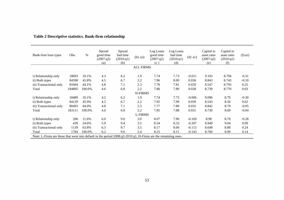
53

Table 2 Descriptive statistics. Bank-firm relationship

Bank-firm loan types

Obs.

%

Spread good time(2007:q2)

(a)

Spread bad time (2010:q1)

(b)

(b) -(a)

Log Loans good time (2007:q2)

(c )

Log Loansbad time (2010:q1)

(d)

(d) -(c)

Capital to asset ratio(2007:q2)

(e)

Capital to asset ratio (2010:q1)

(f)

(f)-(e)

ALL FIRMS i) Relationship only 18693 10.1% 4.3 6.2 1.9 7.74 7.73 -0.011 9.103 8.794 -0.31 ii) Both types 84598 45.8% 4.5 6.7 2.2 7.96 8.00 0.036 8.843 8.743 -0.10 iii) Transactional only 81604 44.1% 4.8 7.1 2.3 7.78 7.81 0.029 8.547 8.793 0.25 Total 184895 100.0% 4.6 6.8 2.2 7.86 7.89 0.028 8.739 8.770 0.03

H-FIRMS i) Relationship only 18489 10.1% 4.2 6.2 1.9 7.74 7.73 -0.006 9.096 8.79 -0.30 ii) Both types 84129 45.9% 4.5 6.7 2.2 7.95 7.99 0.039 8.543 8.56 0.02 iii) Transactional only 80493 44.0% 4.8 7.1 2.3 7.77 7.80 0.032 8.842 8.79 -0.05 Total 183111 100.0% 4.6 6.8 2.2 7.85 7.88 0.031 8.730 8.69 -0.04

L-FIRMS i) Relationship only 206 11.6% 6.0 9.0 3.0 8.07 7.90 -0.169 8.98 8.70 -0.28 ii) Both types 439 24.6% 5.9 9.4 3.5 8.54 8.33 -0.207 8.949 9.04 0.09 iii) Transactional only 1139 63.8% 6.3 9.7 3.5 8.17 8.06 -0.113 8.648 8.88 0.24 Total 1784 100.0% 6.2 9.6 3.4 8.25 8.11 -0.143 8.760 8.90 0.14 Note: L-Firms are those that went into default in the period 2008:q3-2010:q1, H-Firms are the remaining ones.

54

Table 3 Effect of Bank-firm relationship on the marginal probability of a firm’s default

Dependent variable: P(defaultk=1)

(I) Baseline equation

(II) Firm specific characteristics

(III) Alternative

Weight

Coef. Sig. Coef. Sig. Coef. Sig.

T-share (in value) 0.0032 *** 0.0029 ***

(0.0008) (0.0007) T-share (number of banks) 0.0028 ***

(0.0007) 0.0051 *** 0.0051 *** (0.0005) (0.0001) LTD -0.0002 -0.0002

(0.0018) (0.0018) Small firm -0.0021 -0.0021

(0.0034) (0.0034) CREDIT_HISTORY -0.0002 *** -0.0001 *** (0.0000) (0.0000) Bank fixed effects Yes Yes Yes

Industry-province dummies Yes Yes Yes

Number of obs. 72,489 72,489 72,489

Pseudo R2 0.1273 0.1395 0.1397

The models estimate the marginal probability for a firm k to go into default in the period 2008:q3-2010:q1. All explanatory variables are evaluated at 2008:q2, prior Lehman's default. The variable T- Share indicates the proportion of loans that firm k has borrowed from a transactional bank. We report the share both in loan value and in terms of number of T-banks. Parameter estimates are reported with robust standard errors in brackets (cluster at individual bank level). The symbols *, **, and *** represent significance levels of 10%, 5%, and 1% respectively. Coefficients for industry-province dummies and bank fixed effects are not reported.

55

Table 4 T-banking and R-banking in good times and bad times

Variables

Interest rate good time (2007:q2)

(I)

Interest rate bad time (2010:q1)

(II)

Log Loans good time (2007:q2)

(III)

Log Loans bad time (2010:q1)

(IV) T-Bank -0.0805*** 0.1227*** -0.2753*** -0.3129*** (0.0174) (0.0210) (0.0123) (0.0110) Bank fixed effects yes yes yes yes Firm fixed effects yes yes yes yes Number of obs. 184,859 184,859 184,859 184,859 Adjusted R-squared 0.529 0.585 0.426 0.473 Notes: The models in column (I) and (III) are estimated in 2007:q2; those in columns (II) and (IV) in 2010:q1. The dummy T-Bank takes the value of 1 if the lending relationship is with a transactional bank. The coefficients represent the difference relative to relationship banking (R-banks). Parameter estimates are reported with robust standard errors in brackets (cluster at individual firm level). The symbols *, **, and *** represent significance levels of 10%, 5%, and 1% respectively. Coefficients for fixed effects are not reported.

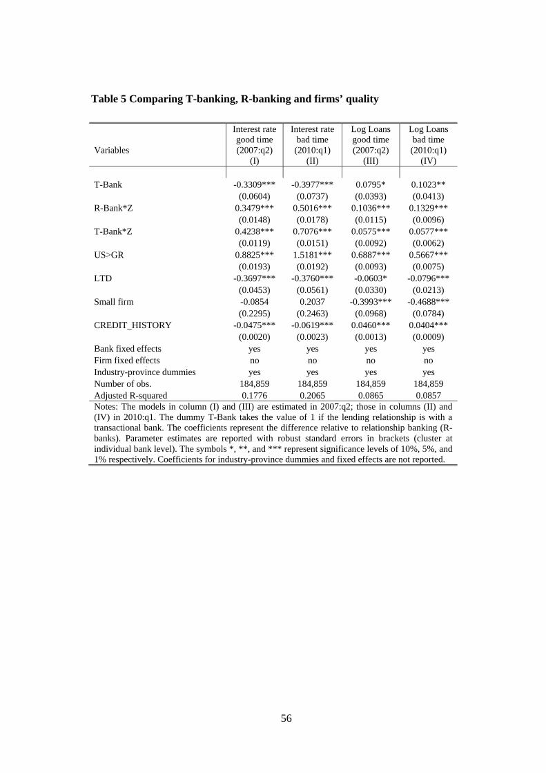
56

Table 5 Comparing T-banking, R-banking and firms’ quality

Variables

Interest rategood time (2007:q2)

(I)

Interest ratebad time (2010:q1)

(II)

Log Loans good time (2007:q2)

(III)

Log Loans bad time (2010:q1)

(IV) T-Bank -0.3309*** -0.3977*** 0.0795* 0.1023** (0.0604) (0.0737) (0.0393) (0.0413) R-Bank*Z 0.3479*** 0.5016*** 0.1036*** 0.1329*** (0.0148) (0.0178) (0.0115) (0.0096) T-Bank*Z 0.4238*** 0.7076*** 0.0575*** 0.0577*** (0.0119) (0.0151) (0.0092) (0.0062) US>GR 0.8825*** 1.5181*** 0.6887*** 0.5667*** (0.0193) (0.0192) (0.0093) (0.0075) LTD -0.3697*** -0.3760*** -0.0603* -0.0796*** (0.0453) (0.0561) (0.0330) (0.0213) Small firm -0.0854 0.2037 -0.3993*** -0.4688*** (0.2295) (0.2463) (0.0968) (0.0784) CREDIT_HISTORY -0.0475*** -0.0619*** 0.0460*** 0.0404*** (0.0020) (0.0023) (0.0013) (0.0009) Bank fixed effects yes yes yes yes Firm fixed effects no no no no Industry-province dummies yes yes yes yes Number of obs. 184,859 184,859 184,859 184,859 Adjusted R-squared 0.1776 0.2065 0.0865 0.0857 Notes: The models in column (I) and (III) are estimated in 2007:q2; those in columns (II) and (IV) in 2010:q1. The dummy T-Bank takes the value of 1 if the lending relationship is with a transactional bank. The coefficients represent the difference relative to relationship banking (R-banks). Parameter estimates are reported with robust standard errors in brackets (cluster at individual bank level). The symbols *, **, and *** represent significance levels of 10%, 5%, and 1% respectively. Coefficients for industry-province dummies and fixed effects are not reported.

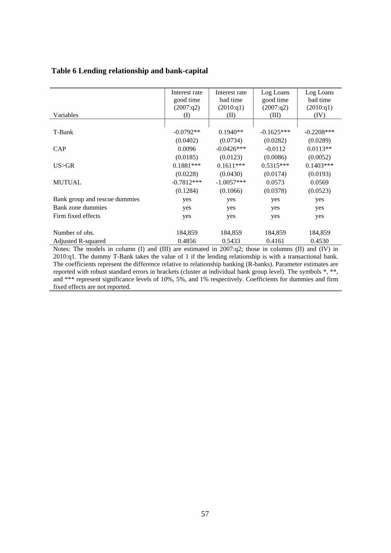
57

Table 6 Lending relationship and bank-capital

Variables

Interest rate good time (2007:q2)

(I)

Interest rate bad time (2010:q1)

(II)

Log Loans good time (2007:q2)

(III)

Log Loans bad time (2010:q1)

(IV) T-Bank -0.0792** 0.1940** -0.1625*** -0.2208*** (0.0402) (0.0734) (0.0282) (0.0289) CAP 0.0096 -0.0426*** -0.0112 0.0113** (0.0185) (0.0123) (0.0086) (0.0052) US>GR 0.1881*** 0.1611*** 0.5315*** 0.1403*** (0.0228) (0.0430) (0.0174) (0.0193) MUTUAL -0.7812*** -1.0057*** 0.0573 0.0569 (0.1284) (0.1066) (0.0378) (0.0523) Bank group and rescue dummies yes yes yes yes Bank zone dummies yes yes yes yes Firm fixed effects yes yes yes yes Number of obs. 184,859 184,859 184,859 184,859 Adjusted R-squared 0.4856 0.5433 0.4161 0.4530 Notes: The models in column (I) and (III) are estimated in 2007:q2; those in columns (II) and (IV) in 2010:q1. The dummy T-Bank takes the value of 1 if the lending relationship is with a transactional bank. The coefficients represent the difference relative to relationship banking (R-banks). Parameter estimates are reported with robust standard errors in brackets (cluster at individual bank group level). The symbols *, **, and *** represent significance levels of 10%, 5%, and 1% respectively. Coefficients for dummies and firm fixed effects are not reported.

58

Table 7 Capital endowment and bank type

Variables

Baseline model

(I)

Bank-specific characteristics

(II)

Firm-specific characteristics

(III)

Financially constrained

firms (IV)

T-share -3.839*** -3.276** -3.091** -3.203** (0.890) (1.301) (1.267) (1.265) Bank size -0.040 0.090 0.092 (0.280) (0.268) (0.264) Bank liquidity ratio -0.009 -0.011 -0.003 (0.016) (0.019) (0.017) Retail ratio 0.049*** 0.031* 0.029* (0.017) (0.017) (0.017) Proportion of small firms in the bank’s credit portfolio 6.169 5.972 (4.248) (4.115) Proportion of LTD firms in the bank’s credit portfolio -2.422 -2.141 (3.723) (3.712) Average Z-score of the bank’s credit portfolio -1.611 -1.337 (2.468) (2.563) Proportion of financially constrained firms (US>GR) 5.392 (6.603) Bank zone dummies yes yes yes yes Number of obs. 179 179 179 179 Adjusted R-squared 0.130 0.185 0.217 0.218 Notes: The dependent variable is the regulatory capital/risk-weighted asset ratio at 2008:q2 prior to Lehman’s default. The variable T-share represents the proportion of transactional loans (in value) for bank j. It takes the value from 0 (pure R-bank) to 1 (pure T-bank). All bank-specific characteristics and credit portfolio characteristic are at 2008:q1. Parameter estimates are reported with robust standard errors in brackets (cluster at individual bank level). The symbols *, **, and *** represent significance levels of 10%, 5%, and 1% respectively. Coefficients for bank zone dummies are not reported.

59

Table C1 Effect of Bank-firm relationship on the marginal probability of a firm’s default. Including Main bank dummy and its interaction with T-share.

Dependent variable: P(defaultk=1)

(I) Baseline equation

(II) Firm specific characteristics

(III) Alternative

Weight

Coef. Sig. Coef. Sig. Coef. Sig.

T-share (in value) 0.0042 *** 0.0036 ***

(0.0011) (0.0009) T-share (number of banks) 0.0036 ***

(0.0015) Maxsh -0.0123 *** -0.0108 *** -0.0106 *** (0.0022) (0.0018) (0.0019) Maxsh*T-share(in value) -0.0041 * -0.0033 *

(0.0023) (0.0019) Maxsh*T-share(number of banks) -0.0035 *

(0.0020) 0.0048 *** 0.0048 *** (0.0004) (0.0004) LTD -0.0006 -0.0006

(0.0017) (0.0017) Small firm -0.0020 -0.0020

(0.0032) (0.0032) CREDIT_HISTORY -0.0002 *** -0.0002 *** (0.0001) (0.0001) Bank fixed effects Yes Yes Yes

Industry-province dummies Yes Yes Yes

Number of obs. 72,489 72,489 72,489

Pseudo R2 0.0782 0.1190 0.1190 The models estimate the marginal probability for a firm k to go into default in the period 2008:q3-2010:q1. All explanatory variables are evaluated at 2008:q2, prior Lehman's default. The variable T- Share indicates the proportion of loans that firm k has borrowed from a transactional bank. We report the share both in loan value and in terms of number of T-banks. The variable Maxsh indicates the highest share of lending that is granted by the main bank. Parameter estimates are reported with robust standard errors in brackets (cluster at individual bank level). The symbols *, **, and *** represent significance levels of 10%, 5%, and 1% respectively. Coefficients for industry-province dummies and bank fixed effects are not reported.

60

Table C2 T-banking and R-banking in good times and bad times. Including Main bank dummy and its interaction with T-bank.

Variables

Interest rate good time (2007:q2)

(I)

Interest rate bad time (2010:q1)

(II)

Log Loans good time (2007:q2)

(III)

Log Loans bad time (2010:q1)

(IV) T-Bank -0.0896*** 0.1086*** -0.1504*** -0.2067*** (0.0201) (0.0243) (0.0121) (0.0116) Main -0.0969*** -0.1705*** 1.1652*** 0.8594*** (0.0232) (0.0281) (0.0130) (0.0130) Main*T-Bank -0.0080 -0.0233 0.0325 0.0125 (0.0301) (0.0361) (0.0366) (0.0164) Bank fixed effects yes yes yes yes Firm fixed effects yes yes yes yes Number of obs. 184,859 184,859 184,859 184,859 Adjusted R-squared 0.529 0.586 0.585 0.570 Notes: The models in column (I) and (III) are estimated in 2007:q2; those in columns (II) and (IV) in 2010:q1. The dummy T-Bank takes the value of 1 if the lending relationship is with a transactional bank. The coefficients represent the difference relative to relationship banking (R-banks). The dummy Main is equal to one if that bank grants the highest share of lending to that firm. Parameter estimates are reported with robust standard errors in brackets (cluster at individual firm level). The symbols *, **, and *** represent significance levels of 10%, 5%, and 1% respectively. Coefficients for fixed effects are not reported.

61

Table C3 Effect of Bank-firm relationship on the marginal probability of a firm’s default. Changing relationship lending definition from province to region.

Dependent variable: P(defaultk=1)

(I) Baseline equation

(II) Firm specific characteristics

(III) Alternative

Weight

Coef. Sig. Coef. Sig. Coef. Sig.

T-share (in value) 0.0024 *** 0.0024 ***

(0.0007) (0.0007) T-share (number of banks) 0.0034 ***

(0.0007) 0.0051 *** 0.0051 *** (0.0004) (0.0004) LTD -0.0002 -0.0002

(0.0018) (0.0018) Small firm -0.0020 -0.0018

(0.0034) (0.0035) CREDIT_HISTORY -0.0001 ** -0.0002 ** (0.0000) (0.0000) Bank fixed effects Yes Yes Yes

Industry-province dummies Yes Yes Yes

Number of obs. 72,489 72,489 72,489

Pseudo R2 0.0612 0.1004 0.1003

The models estimate the marginal probability for a firm k to go into default in the period 2008:q3-2010:q1. All explanatory variables are evaluated at 2008:q2, prior Lehman's default. The variable T- Share indicates the proportion of loans that firm k has borrowed from a transactional bank. We report the share both in loan value and in terms of number of T-banks. Parameter estimates are reported with robust standard errors in brackets (cluster at individual bank level). The symbols *, **, and *** represent significance levels of 10%, 5%, and 1% respectively. Coefficients for industry-province dummies and bank fixed effects are not reported.

62

Table C4 T-banking and R-banking in good times and bad times. Changing relationship lending definition from province to region.

Variables

Interest rate good time (2007:q2)

(I)

Interest rate bad time (2010:q1)

(II)

Log Loans good time (2007:q2)

(III)

Log Loans bad time (2010:q1)

(IV) T-Bank -0.0748*** 0.1038*** -0.2428*** -0.256*** (0.0182) (0.0217) (0.0123) (0.0110) Bank fixed effects yes yes yes yes Firm fixed effects yes yes yes yes Number of obs. 184,859 184,859 184,859 184,859 Adjusted R-squared 0.529 0.585 0.426 0.472 Notes: The models in column (I) and (III) are estimated in 2007:q2; those in columns (II) and (IV) in 2010:q1. The dummy T-Bank takes the value of 1 if the lending relationship is with a transactional bank. The coefficients represent the difference relative to relationship banking (R-banks). Parameter estimates are reported with robust standard errors in brackets (cluster at individual firm level). The symbols *, **, and *** represent significance levels of 10%, 5%, and 1% respectively. Coefficients for fixed effects are not reported.

63

Table C5 Effect of Bank-firm relationship on the marginal probability of a firm’s default. All foreign banks subsidiaries are T-banks.

Dependent variable: P(defaultk=1)

(I) Baseline equation

(II) Firm specific characteristics

(III) Alternative

Weight

Coef. Sig. Coef. Sig. Coef. Sig.

T-share (in value) 0.0031 *** 0.0027 ***

(0.0009) (0.0007) T-share (number of banks) 0.0027 ***

(0.0007) 0.0051 *** 0.0051 *** (0.0004) (0.0004) LTD -0.0002 -0.0002

(0.0018) (0.0018) Small firm -0.0021 -0.0021

(0.0034) (0.0034) CREDIT_HISTORY -0.0002 ** -0.0002 ** (0.0000) (0.0000) Bank fixed effects Yes Yes Yes

Industry-province dummies Yes Yes Yes

Number of obs. 72,489 72,489 72,489

Pseudo R2 0.0600 0.0994 0.0994

The models estimate the marginal probability for a firm k to go into default in the period 2008:q3-2010:q1. All explanatory variables are evaluated at 2008:q2, prior Lehman's default. The variable T- Share indicates the proportion of loans that firm k has borrowed from a transactional bank. We report the share both in loan value and in terms of number of T-banks. Parameter estimates are reported with robust standard errors in brackets (cluster at individual bank level). The symbols *, **, and *** represent significance levels of 10%, 5%, and 1% respectively. Coefficients for industry-province dummies and bank fixed effects are not reported.

64

Table C6 T-banking and R-banking in good times and bad times. All foreign

banks subsidiaries are T-banks.

Variables

Interest rate good time (2007:q2)

(I)

Interest rate bad time (2010:q1)

(II)

Log Loans good time (2007:q2)

(III)

Log Loans bad time (2010:q1)

(IV) T-Bank -0.0844*** 0.1030*** -0.2737*** -0.2970*** (0.0180) (0.0218) (0.0128) (0.0115) Bank fixed effects yes yes yes yes Firm fixed effects yes yes yes yes Number of obs. 184,859 184,859 184,859 184,859 Adjusted R-squared 0.529 0.585 0.426 0.473 Notes: The models in column (I) and (III) are estimated in 2007:q2; those in columns (II) and (IV) in 2010:q1. The dummy T-Bank takes the value of 1 if the lending relationship is with a transactional bank. The coefficients represent the difference relative to relationship banking (R-banks). Parameter estimates are reported with robust standard errors in brackets (cluster at individual firm level). The symbols *, **, and *** represent significance levels of 10%, 5%, and 1% respectively. Coefficients for fixed effects are not reported.

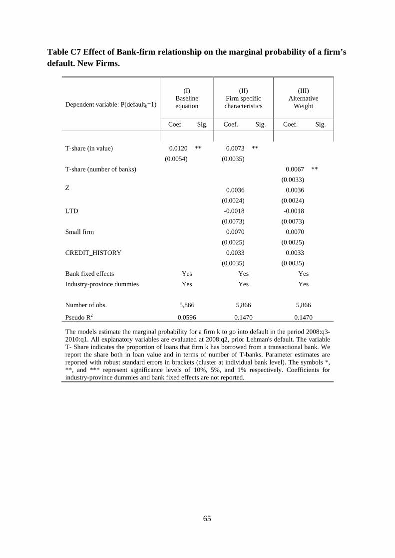
65

Table C7 Effect of Bank-firm relationship on the marginal probability of a firm’s default. New Firms.

Dependent variable: P(defaultk=1)

(I) Baseline equation

(II) Firm specific characteristics

(III) Alternative

Weight

Coef. Sig. Coef. Sig. Coef. Sig.

T-share (in value) 0.0120 ** 0.0073 **

(0.0054) (0.0035)

T-share (number of banks) 0.0067 **

(0.0033) 0.0036 0.0036 (0.0024) (0.0024)

LTD -0.0018 -0.0018

(0.0073) (0.0073)

Small firm 0.0070 0.0070

(0.0025) (0.0025)

CREDIT_HISTORY 0.0033 0.0033 (0.0035) (0.0035)

Bank fixed effects Yes Yes Yes

Industry-province dummies Yes Yes Yes

Number of obs. 5,866 5,866 5,866

Pseudo R2 0.0596 0.1470 0.1470

The models estimate the marginal probability for a firm k to go into default in the period 2008:q3-2010:q1. All explanatory variables are evaluated at 2008:q2, prior Lehman's default. The variable T- Share indicates the proportion of loans that firm k has borrowed from a transactional bank. We report the share both in loan value and in terms of number of T-banks. Parameter estimates are reported with robust standard errors in brackets (cluster at individual bank level). The symbols *, **, and *** represent significance levels of 10%, 5%, and 1% respectively. Coefficients for industry-province dummies and bank fixed effects are not reported.

66

Table C8 T-banking and R-banking in good times and bad times. New Firms.

Variables

Interest rate good time (2007:q2)

(I)

Interest rate bad time (2010:q1)

(II)

Log Loans good time (2007:q2)

(III)

Log Loans bad time (2010:q1)

(IV) T-Bank -0.0844*** 0.1030*** -0.2737*** -0.2970*** (0.0180) (0.0218) (0.0128) (0.0115) Bank fixed effects yes yes yes yes Firm fixed effects yes yes yes yes Number of obs. 5,866 5,866 5,866 5,866 Adjusted R-squared 0.529 0.585 0.426 0.473 Notes: The models in column (I) and (III) are estimated in 2007:q2; those in columns (II) and (IV) in 2010:q1. The dummy T-Bank takes the value of 1 if the lending relationship is with a transactional bank. The coefficients represent the difference relative to relationship banking (R-banks). Parameter estimates are reported with robust standard errors in brackets (cluster at individual firm level). The symbols *, **, and *** represent significance levels of 10%, 5%, and 1% respectively. Coefficients for fixed effects are not reported.