RELATED INTERPRETATIONS OF ELLIPTIC CURVES

RELATED INTERPRETATIONS OF ELLIPTIC CURVES

ALEKSANDER SKENDERI

Abstract. The goal of this expository paper is to explore the relations be-

tween many interpretations of elliptic curves over C. Introducing elliptic curves

as algebraic varieties, we then discuss their algebraic interpretation as groups,their topological interpretation as complex tori, and briefly also mention the

complex analytic structures that they possess. Thus the study of elliptic curves

serves as a beautiful representation of the unity of mathematics, using toolsfrom algebra, topology, and analysis. This paper assumes a good familiarity

with fundamental ideas in algebra, complex analysis, and hyperbolic geometry.

Contents

1. Introduction 12. The Group Law on Elliptic Curves 22.1. Preliminaries on Algebraic Plane Curves 22.2. Lattices and Fundamental Regions 22.3. Basic Results on Elliptic Functions 42.4. An Addition Theorem and the Group Law 93. Complex Tori and Elliptic Curves 113.1. Tori and Moduli 123.2. The Modular Function 133.3. The Lattice Associated to a Cubic 15Acknowledgments 20References 20

1. Introduction

The study of elliptic curves is interesting for many reasons. One such reasonis the incredible role they play in modern mathematics, such as in the proofs ofthe Modularity Theorem and Fermat’s Last Theorem. Another reason, that whichconcerns this paper, is that the study of elliptic curves serves to relate many differentbranches of mathematics; indeed, algebra, analysis, and topology all play a rolein the study of elliptic curves. The goal of this paper is to precisely elucidatethese relations. Beginning with the definition of an elliptic curve as the zero setof a particular polynomial, we then discuss how elliptic curves can be thought ofas groups and complex tori, and briefly also discuss the analytic structures theypossess.

1

2 ALEKSANDER SKENDERI

2. The Group Law on Elliptic Curves

2.1. Preliminaries on Algebraic Plane Curves. Let k be a field of character-istic different from 2 or 3, and define the affine plane A2

k to be the set of all points(a, b) with a, b ∈ k. An affine plane curve is the collection of all points (x, y) in A2

k

that satisfy

f(x, y) = 0,(2.1)

for some nonconstant polynomial f ∈ k[x, y]. Typically, the field k we will beworking with will be either R or C. The degree of the polynomial f in (2.1) is alsocalled the degree of the curve. A degree 2 curve is called a conic and a degree 3curve is called a cubic. In the Euclidean space R2, the familiar examples of conicsare the parabola, ellipse, and hyperbola. We will be primarily interested in cubics;in particular, in a special type of cubic called an elliptic curve. We first need thefollowing definition.

Definition 2.2. A point P is a singular point or singularity of the affine curvedefined by f(x, y) = 0 if

∂f

∂x(P ) =

∂f

∂y(P ) = 0.

A point is nonsingular if it is not singular, and a curve all of whose points arenonsingular is called nonsingular or smooth.

Definition 2.3. An elliptic curve is the set of points defined by an equation of theform

y2 = x3 + ax+ b,

where the cubic f(x, y) = y2 − x3 − ax− b is nonsingular.

A priori it is not intuitively clear that one can impose a group law on such acurve. Our present goal is to show how this is possible.

2.2. Lattices and Fundamental Regions. Let f be a function defined on thecomplex plane C. A complex number ω ∈ C is called a period of f if

f(z + ω) = f(z)

for all z ∈ C. The function f is called periodic if it has a period ω 6= 0. Familiarexamples of periodic functions are sinz and cosz, which have a period 2π, and theexponential function ez, which has a period 2πi. The set of periods of each of thesefunctions is of the form Ω = nω : n ∈ Z, for some fixed ω ∈ C \ 0, and istherefore isomorphic to the integers Z. The functions we are presently interestedin will have their set of periods of the form

Ω(ω1, ω2) = nω1 +mω2 : n,m ∈ Z,

for some fixed ω1, ω2 ∈ C \ 0, where ω1 and ω2 are linearly independent over R;such a set is called a lattice. Notice that Ω(ω1, ω2) ∼= Z × Z. If f contains somelattice in its set of periods, then f is said to be doubly periodic. Currently, our onlyexample of doubly periodic functions are the constant functions. It is a nontrivialtask to construct nonconstant doubly periodic functions, as we shall soon see. Wefirst discuss a few more properties of lattices. If Ω(ω1, ω2) has the set ω1, ω2

RELATED INTERPRETATIONS OF ELLIPTIC CURVES 3

as a basis, it is clear that it can have many other types of bases. For instance,ω1 + ω2, ω2 is also a basis, since if ω ∈ Ω(ω1, ω2), then

ω = nω1 +mω2 = n(ω1 + ω2) + (m− n)ω2,

where n,m − n ∈ Z. The following simple exercise in linear algebra explains howwe find other bases in more generality.

Lemma 2.4. Let a, b, c, and d be integers and let Ω(ω1, ω2) be a lattice. Theequations

ω′2 = aω2 + bω1

ω′1 = cω2 + dω1

define a basis for Ω(ω1, ω2) if and only if ad− bc = ±1.

Proof. See section 3.4 of [1].

Given a lattice Ω, we say that z1, z2 ∈ C are congruent mod Ω, written z1 ∼ z2

mod Ω (or simply z1 ∼ z2) if z1 − z2 ∈ Ω. This is easily seen to be an equivalencerelation, with the equivalence classes being the cosets z + Ω of the subgroup Ω ofthe additive group C. Since each ω ∈ Ω induces the translation tω : z 7→ z + ω ofC, and since tω1+ω2

= tω1 tω2

we have a group isomorphism Ω ∼= tω : ω ∈ Ω.Hence, two points of C are congruent mod Ω if and only if they lie in the sameorbit under the action of Ω on C.

Definition 2.5. A closed, connected subset P of C is said to be a fundamental regionfor Ω if

(i) for each z ∈ C, P contains at least one point in the same Ω-orbit as z, and(ii) no two points in the interior of P are in the same Ω-orbit.

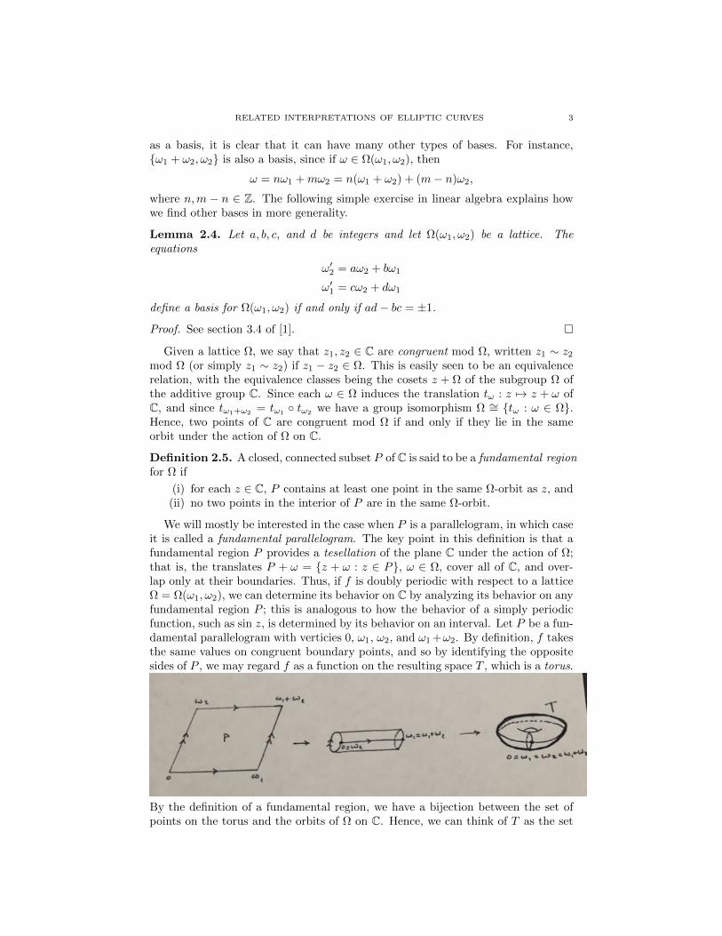
We will mostly be interested in the case when P is a parallelogram, in which caseit is called a fundamental parallelogram. The key point in this definition is that afundamental region P provides a tesellation of the plane C under the action of Ω;that is, the translates P + ω = z + ω : z ∈ P, ω ∈ Ω, cover all of C, and over-lap only at their boundaries. Thus, if f is doubly periodic with respect to a latticeΩ = Ω(ω1, ω2), we can determine its behavior on C by analyzing its behavior on anyfundamental region P ; this is analogous to how the behavior of a simply periodicfunction, such as sin z, is determined by its behavior on an interval. Let P be a fun-damental parallelogram with verticies 0, ω1, ω2, and ω1 +ω2. By definition, f takesthe same values on congruent boundary points, and so by identifying the oppositesides of P , we may regard f as a function on the resulting space T , which is a torus.

By the definition of a fundamental region, we have a bijection between the set ofpoints on the torus and the orbits of Ω on C. Hence, we can think of T as the set


of Ω-orbits on C; that is T is the collection of cosets C/Ω. Since C is abelian, thesubgroup Ω is normal, and thus T = C/Ω has the structure of an abelian group.Furthermore, T is compact since the function that identifies boundary points is acontinuous function from the compact set P onto T .

2.3. Basic Results on Elliptic Functions.

Definition 2.6. A meromorphic function f : C → Σ := C ∪ ∞ is elliptic withrespect to a lattice Ω ⊂ C if f is doubly periodic with respect to Ω. 1

If f is elliptic with respect to Ω, then our previous discussion shows that wemay regard f as a function f : T → Σ, where T is the torus T = C/Ω. Fix c ∈ Σand suppose f is not identically equal to c. As f is meromorphic, the solutionsof f(z) = c must be isolated, and each solution must have finite multiplicity, withcongruent solutions z1, z2 ∈ C having the same multiplicity (i.e., they are zeroes ofthe same order for the function g(z) = f(z)−c). If P is a fundamental parallelogramfor Ω, then the compactness of P and the fact that the solutions of f(z) = c areisolated shows that P contains only finitely many of these solutions. By replacingP by P +w (w ∈ C) if necessary, we can assume that there are no solutions on theboundary ∂P of P . Let the solutions within P be z = z1, ..., zn, with multiplicitiesk1, ..., kn. Set N = k1 + ...+kn. Then there are N solutions, counting multiplicities,of f(z) = c within P . As z1, ..., zn are representatives for the congruence classes ofsolutions of f(z) = c for z ∈ C, we may view N as the sum of the multiplicities of thesolutions of f([z]) = c, where [z] ∈ T = C/Ω is the congruence class correspondingto z ∈ C. This leads to the following definition.

Definition 2.7. The order ord(f) of an elliptic function f : C/Ω → Σ is thenumber of solutions, counting multiplicites, of f([z]) =∞; that is, it is the sum ofthe orders of the congruence classes of the poles of f .

For the following theorems, we assume that f is elliptic with respect to Ω =Ω(ω1, ω2), that ord(f) = N , and that P is a fundamental parallelogram for Ωhaving verticies t, t + ω1, t + ω2, t + ω1 + ω2, where t ∈ C is chosen so that ∂Pcontains no zeroes or poles of f .

Theorem 2.8. The function f is constant if and only if N = 0 (in particular, anyanalytic elliptic function must be constant).

Proof. If f is constant, then it is analytic. Hence it has no poles in C, and thusN = 0. Conversely, suppose that N = 0, so that f has no poles in C, and istherefore analytic. By the definition of P , we have f(P ) = f(C). As P is compactand f is continuous, f(P ) ⊂ C is compact, and therefore bounded. Hence f is abounded, entire function on C, whence Liouville’s theorem implies that f must beconstant.

Theorem 2.9. The sum of the residues of f within P is zero.

Proof. Since f is meromorphic and ∂P was chosen so as not to contain any ze-roes or poles of f , we see that the sum of the residues of f within P is given by

12πi

∫∂P

f(z)dz. Let Γ1,Γ2,Γ3, and Γ4 be the sides of P connecting t and t + ω1,

1For a historical perspective on elliptic functions, see section 3.6 of [1].


t + ω1 and t + ω1 + ω2, t + ω1 + ω2 and t + ω2, and t, respectively, so that theorientation of ∂P is the counterclockwise (positive) orientation. Then,

1

2πi

∫∂P

f(z)dz =1

2πi

4∑k=1

∫Γk

f(z)dz.(2.10)

Now as ω2 is a period of f and Γ3 = Γ1 +ω2 with the reverse orientation, we obtain∫Γ1

f(z)dz =

∫Γ1

f(z + ω2)dz = −∫

Γ3

f(z + ω2)d(z + ω2) = −∫

Γ3

f(z)dz,

where in the last equality, with an abuse of notation, we performed a change of vari-ables setting z−ω2 for z. A similar argument shows that

∫Γ2f(z)dz = −

∫Γ4f(z)dz.

By (2.10), we see that the sum of the residues of f within P is zero.

Corollary 2.11. There are no elliptic functions of order N = 1.

Proof. If f were an elliptic function of order N = 1, then f would have a singleresidue of order 1 at some point z0 ∈ P . In some small neighborhood of z0, thefunction f then has a Laurent series expansion

f(z) =

∞∑n=−1

an(z − z0)n,

where a−1 6= 0. Then the sum of the resides of f within P is a−1 6= 0, contradictingthe preceding theorem.

Theorem 2.12. If f has order N > 0, then f takes each value c ∈ Σ exactly Ntimes.

Proof. If c = ∞, then this is just the definition of N ; assume then that c ∈ C.Replacing f by f − c (which has the same order as f), we may assume that c = 0.Now f ′/f is meromorphic and ∂P contains no zeroes or poles of f , so that f ′/f isanalytic on ∂P . Furthermore, since f is elliptic, so is f ′, and thus so is the quotientf ′/f . Thus integrating f ′/f around ∂P and applying the argument of Theorem2.9, we see that ∫

∂P

f ′(z)

f(z)dz = 0.

By Cauchy’s Argument Principle, we conclude that f has the same number ofzeroes as its number of poles, counting multiplicities. Thus, f(z) = 0 has exactlyN solutions, as desired.

Corollary 2.11 tells us that if we want nonconstant elliptic functions, then theymust have order at least 2. Just as how the familiar trigonometric and exponentialfunctions are obtained by means of power series, elliptic functions will be obtainedby means of power series; the only difference now is that the indexing set is somelattice Ω = Ω(ω1, ω2). As the series we consider are typically absolutely convergent,they are invariant under rearrangements, and so the particular order of the seriesis not essential. It is not too difficult to construct elliptic functions of order N ≥ 3,as the following theorem shows.

Theorem 2.13. For each integer N ≥ 3, the function FN (z) =∑ω∈Ω(z − ω)−N

is elliptic of order N with respect to Ω.


Proof. See Theorem 3.9.3 of [1].

The proof is primarily based upon the fact for s ∈ R, the series∑ω∈Ω\0 |ω|−s

converges if and only if s > 2 (notice the similarity with how the series∑n∈N\0 |n|−s

converges if and only if s > 1). Thus, in order to obtain elliptic functions of order2, we need to subtract an additional term from the summand to guarantee absoluteconvergence.

Definition 2.14. The Weierstrass ℘ function associated to a lattice Ω, denotedby ℘(z,Ω) (or just ℘(z), when the lattice is understood) is defined by

℘(z) =1

z2+

∑ω∈Ω\0

(1

(z − ω)2− 1

ω2

).(2.15)

We now show that this represents an elliptic function of order 2. One shows thatthis series represents a well-defined meromorphic function by comparing it with theseries

∑ω∈Ω\0 |ω|−3 in a similar fashion to the argument of Theorem 2.13. In

particular, this argument shows that it is uniformly convergent on compact subsetsof C, so that we can differentiate and integrate this series term-by-term. A moreinteresting question is how one shows that it is elliptic. Indeed, this is not clear apriori, as the series is not of the form

∑ω∈Ω f(z − ω). Our method is based upon

relating ℘ to one of the series FN (z) mentioned above.

Theorem 2.16. The function ℘(z) is an elliptic function with Ω as its lattice Ω℘of periods.

Proof. We described above how to show that ℘(z) is meromorphic, so we only showthat Ω = Ω℘. As the series (2.15) defining ℘(z) is uniformly convergent on compactsubsets of C, we can differentiate term-by-term to obtain

℘′(z) =−2

z3−

∑ω∈Ω\0

(2

(z − ω)3

)= −2

∑ω∈Ω

1

(z − ω)3= −2F3(z),

where F3(z) is elliptic of order 3 by Theorem 2.13. We conclude that for eachω ∈ Ω, ℘′(z + ω)− ℘′(z) = 0, so that ℘(z +w)− ℘(z) is some constant cω. Settingz = −ω/2 and noticing that ℘(z) is even, we find that

cω = ℘(ω

2

)− ℘

(− ω

2

)= 0,

showing that each ω ∈ Ω is a period of ℘(z). Thus, Ω ⊂ Ω℘. To prove the reverseinclusion, we notice that since 0 is a pole of ℘(z), there is a pole of ℘(z) at everypoint in Ω℘. But the expression for ℘(z) shows that it has no poles in C\Ω. Hence,Ω℘ ⊂ Ω.

Theorem 2.17. ℘(z) has order 2 and ℘′(z) has order 3.

Proof. ℘(z) has a pole of order 2 at each lattice point and no other poles. Thus ithas a single congruence class of poles of order 2, showing that it has order 2. Inthe above proof, we saw that ℘′(z) = −2F3(z). Since F3(z) has a single congruenceclass of poles of order 3, ℘′(z) has order 3.

It is a theorem that the field of all even elliptic functions over C is preciselythe field of rational functions in ℘(z), and that the field of all elliptic functionsover C is the field of rational functions in ℘(z) and ℘′(z) (see Theorem 3.11.1 of


[1]). Thus, just as every simply periodic meromorphic function has a Fourier seriesexpansion in terms of sin(z) and cos(z) (with even functions being expressed solelyin terms of cos(z)), where sin(z) and cos(z) are related by sin′(z) = cos(z), we havesimilar results for elliptic functions. We also know that sin(z) and cos(z) satisfythe algebraic equation x2 + y2 − 1 = 0, where x = cos(z) and y = sin(z). It is thennatural to ask whether ℘(z) and ℘′(z) satisfy a similar equation. Moreover, sincethe algebraic equation relating sin(z) and cos(z) is what gives us parametrizationsof conics such as the circle and (more generally) the ellipse, we should be hopefulthat if we find an algebraic equation connecting ℘(z) and ℘′(z), then we mightbe able to parametrize some type of plane curve. We now derive the differentialequation relating ℘(z) and ℘′(z), and then explain how this allows us to induce thegroup law on an elliptic curve.

To derive this equation, we need to find a Laurent series for ℘(z) in a smallneighborhood of z = 0. We begin by obtaining a Laurent series for the function

ζ(z) =1

z+

∑ω∈Ω\0

(1

z − ω+

1

ω+

z

ω2

).(2.18)

Let m = min|ω| : ω ∈ Ω \ 0, and let D = z ∈ C : |z| < m be the largest opendisc centered at zero containing no nonzero lattice point of Ω. Since

1

z − ω+

1

ω+

z

ω2=

z2

ω2(z − ω),

we see by comparison with∑ω∈Ω\0 |ω|−3 that ζ(z) is absolutely convergent for

all z ∈ C \ Ω (and uniformly convergent on compact subsets of C where this seriesis defined, so that it may be differentiated term-by-term). Additionally, for allω ∈ Ω \ 0, the binomial series

1

z − ω= −

∞∑n=1

zn−1

ωn

is absolutely convergent for all z ∈ D. We may then substitute this expression in(2.18) to obtain the Laurent series

ζ(z) =1

z+

∑ω∈Ω\0

(− z2

ω3− z3

ω4− ...

)

=1

z−∞∑n=2

Gn+1zn,

valid for all z ∈ D, where

Gk = Gk(Ω) =∑

ω∈Ω\0

ω−k.

The Gk give what is called the Eisenstein series for Ω. Notice that they are ab-solutely convergent for all k ≥ 3 by Theorem 2.13. For odd k, we have that(−ω)k = −ωk, yielding Gk = 0. The Laurent series for ζ(z) then simplifies to

ζ(z) =1

z−∞∑n=2

G2nz2n−1,


for z ∈ D. Differentiating, we find that

℘(z) = −ζ ′(z) =1

z2+

∞∑n=2

(2n− 1)G2nz2n−2,

yielding a Laurent series for ℘(z), valid for z ∈ D. By explicitly writing out thefirst several terms for the power series ℘′(z)2, 4℘(z)3, and 60G4℘(z), we find that

℘′(z)2 − 4℘(z)3 + 60G4℘(z) + 140G6 = z2φ(z),(2.19)

where φ(z) is some power series convergent in D. Since ℘ and ℘′ are elliptic withrespect to Ω, so is the left hand side of (2.19), which we denote by f(z). Nowf(z) = z2φ(z) in D, and since f(0) = 0, this implies that f vanishes at all ω ∈ Ω.But by construction, f can only have poles at the poles of ℘ or ℘′, which are thelattice points of Ω. Hence f is analytic, and so by Theorem 2.8 f must be constant;this constant is 0 as f(0) = 0. This proves that

Theorem 2.20. ℘′(z)2 = 4℘(z)3 − 60G4℘(z)− 140G6.

It is traditional to write g2(Ω) = g2 for 60G4 and g3(Ω) = g3 for 140G6 so thatthis differential equation becomes

℘′(z)2 = 4℘(z)3 − g2℘(z)− g3.(2.21)

This suggests that we may be able to parametrize the elliptic curve y2 = 4x3 −g2x − g3 by setting x = ℘(z) and y = ℘′(z). To show that we can indeed do this,we need the following results.

Theorem 2.22. Let Ω be a lattice with basis ω1, ω2, and let ω3 = ω1 + ω2. If Pis a fundamental parallelogram for Ω having 0, 1

2ω1,12ω2, and 1

2ω3 in its interior,

then 12ω1,

12ω2, and 1

2ω3 are the zeroes of ℘′ in P .

Proof. By Theorem 2.17, we know that ℘′(z) has three poles and three zeroes in P ,counting multiplicity. Since ℘′(z) is odd, if ω ∈ Ω satisfies 1

2ω ∼ −12ω mod Ω, then

℘′( 12ω) = −℘′( 1

2ω), so that ℘′( 12ω) is either 0 or ∞. Since ℘′ has a pole of order 3

at 0 ∈ P , we conclude that 12ω1,

12ω2, and 1

2ω3 are the zeroes of ℘′ in P .

We now define ej := ℘( 12ωj) for j = 1, 2, 3. As S = [ 1

2ω1] ∪ [ 12ω2] ∪ [ 1

2ω3] is theset of all zeroes of ℘′ in C, we deduce that e1, e2, e3 = ℘(S) is independent of theparticular choice of basis ω1, ω2 of Ω.

Corollary 2.23. For all c ∈ Σ \ e1, e2, e3, the equation ℘(z) = c has two simplesolutions; for c = e1, e2, e3, or ∞, the equation has one double solution.

Proof. By Theorems 2.12 and 2.17, ℘(z) takes each value c ∈ Σ twice, giving eithertwo simple solutions (z and −z, since ℘(z) is even) or one double solution. If c ∈ C,then ℘(z) = c has a double solution if and only if ℘′(z) = 0, so that z ∼ 1

2ωj modΩ (where j = 1, 2, 3), showing that c = ej . If c = ∞, then ℘(z) has a double poleat z = 0, and so ℘(z) =∞ has a double solution.

Theorem 2.24. The values e1, e2, and e3 are mutually distinct.

Proof. Consider fj(z) = ℘(z)− ej for j = 1, 2, 3. Since the poles of the fj are thesame as those of ℘(z), the fj are elliptic functions of order 2 and therefore each hastwo classes of zeroes, counting multiplicities. Since

fj

(1

2ωj

)= f ′j

(1

2ωj

)= 0,


fj has a double class of zeroes on [ 12ωj ] and thus no other zeroes. This implies that

fj(12ωk) 6= 0 for j 6= k; that is, ej 6= ek for j 6= k.

By the differential equation (2.21), we see that the polynomial p(x) = 4x3 −g2x − g3 has its zeroes at the points x = ℘(z) where ℘′(z) = 0. Thus, the aboveresults show that p(x) has the three distinct zeroes e1, e2, and e3.

2.4. An Addition Theorem and the Group Law. From the differential equa-tion (℘′(z))2 = p(℘(z)), where p(x) = 4x3 − g2x − g3, we see that each t ∈ C/Ωdetermines a point (℘(t), ℘′(t)) on the elliptic curve

E = (x, y) ∈ Σ× Σ : y2 = p(x).As we now show, the converse is also true. Moreover, the parametrization of E interms of ℘ and ℘′ shows that E is topologically equivalent (over C, in the analytictopology) to the torus C/Ω. 2

Theorem 2.25. The map θ : C/Ω → E given by θ(t) = (℘(t), ℘′(t)) is a homeo-morphism.

Proof. By Corollary 2.23, we know that t0 = [0] is the only point mapped to(∞,∞) and that tj = [ 1

2ωj ] are the only points mapped to (ej , 0), where j = 1, 2, 3,respectively. If (x, y) ∈ E is any other point, then x 6= ∞, ej and y 6= ∞, 0.Corollary 2.23 then tells us that the equation ℘(t) = x has two simple solutionst = ±t1. As ℘′ is odd, we have that ℘′(t1) = −℘′(−t1) 6= ℘′(−t1) (as t1 6= [ 1

2ωj ]).

Hence, one of either ℘′(t1) or ℘′(−t1) takes the value of y =√p(x) =

√p(℘(t)), so

that one of ±t1 is mapped uniquely onto (x, y) by θ. This shows that θ is a bijection.Finally, as ℘ and ℘′ are meromorphic and nonconstant, they are continuous openmaps; hence so is θ, showing that both θ and θ−1 are continuous.

We saw earlier that T = C/Ω has the structure of an abelian group. If P1 = θ(t1)and P2 = θ(t2) are any two points in E, then we can impose an abelian groupstructure on E by simply defining P1 +P2 = θ(t1 + t2). The above theorem showedthat θ was a bjiection, so that we have forced θ to be an isomorphism. Using this,we see that the identity element on E is

θ([0]) = (℘(0), ℘′(0)) = (∞,∞).

If θ(t) = (x, y) ∈ E, then its inverse is

θ(−t) = (℘(−t), ℘′(−t)) = (℘(t),−℘′(t)) = (x,−y).

If our elliptic curve E were a subset of R2∪(∞,∞) instead of Σ×Σ, then findingthe inverse of (x, y) ∈ E \ (∞,∞) amounts to reflecting the point about thex-axis.

Describing the sum of two points on an elliptic curve in terms of their coordinatesis more difficult. Let Pj = θ(tj), j = 1, 2, be two points on E. Then

P1 + P2 = θ(t1 + t2) = (℘(t1 + t2), ℘′(t1 + t2)).

So as to avoid trivial cases, we assume P1, P2, and P1 +P2 are all non-zero in E. Ifwe can find an addition theorem for the Weierstrass ℘ function, then we can alsoexpress the coordinates of P1 + P2 in terms of those of P1 and P2. Recall that a

2Notice that we have defined E as a subset of Σ × Σ ∼= P1 × P1, instead of as a subset of P2,as it is typically defined. However, in both cases E is the one-point compactification of the finite

part of the elliptic curve, and so the two perspectives can in this way be seen as the same.


function f is said to possess an addition theorem if there exists a non-zero rationalfunction R with complex coefficients in three variables satisfying

R(f(z1), f(z2), f(z1 + z2)) = 0

for all z1, z2 ∈ C (familiar examples of functions possessing addition theoremsinclude the exponential and trigonometric functions). As we already have a differ-ential equation relating ℘ and ℘′, it would be very useful if we could construct anelliptic function g in terms of ℘ and ℘′ that also possesses some relation betweent1, t2, and t1 + t2. For this we need the following theorem, whose proof follows asimilar strategy to that of Theorem 2.12, and is therefore omitted; the interestedreader may consult Theorem 3.6.7 in [1].

Theorem 2.26. Let f be an elliptic function with respect to a lattice Ω havingcongruence classes of zeroes and poles [a1], ..., [ar] and [b1], ..., [bs], with multiplicitiesk1, ..., kr, and l1, ..., ls, respectively. Then,

r∑j=1

kjaj ∼s∑j=1

ljbj mod Ω.

By this theorem, if we can construct an elliptic function g of order 3 having atriple pole at [0] and simple zeroes at t1 and t2 (or a double zero at t1, if t1 = t2),then the third zero t3 of g must satisfy t1 + t2 + t3 = [0]. That is, t3 = −(t1 + t2),and so P1 + P2 = θ(−t3) = (℘(t3),−℘′(t3)). We now construct such a function g.Consider the function

g(t) = ℘′(t)− α℘(t)− β,(2.27)

where α, β ∈ C are to be determined. Then g is certainly elliptic of order 3, andhas a triple pole at [0]. If t1 6= t2, then g has the required zeroes provided that

℘′(tj) = α℘(tj) + β, that is,

yj = αxj + β.(2.28)

where (xj , yj) = (℘(tj), ℘′(tj)) for j = 1, 2. Since t1 + t2 6= [0] by hypothesis, we

have t1 6= ±t2. We also have t1, t2 6= [0], and so x1 and x2 are distinct and finite.Thus we can find α, β ∈ C satisfying (2.28). As t3 = −(t1 + t2) is also a root,(x3, y3) = (℘(t3), ℘′(t3)) also satisfies (2.28). Continuing with the assumption thatt1 6= t2, (2.28) yields

α =y1 − y2

x1 − x2.(2.29)

As y2j = p(xj), we have

p(xj)− (αxj + β)2 = 0,

for j = 1, 2, 3. That is, the xj are the roots of the polynomial

4x3 − α2x2 − (2αβ + g2)x− (β2 + g3) = 0.(2.30)

Using the formula for the sum of the roots, we obtain

x1 + x2 + x3 =α2

4.


Now using (2.29) and that ℘(t1 + t2) = ℘(−(t1 + t2)) = ℘(t3) = x3, we have

℘(t1 + t2) =1

4

(℘′(t1)− ℘′(t2)

℘(t1)− ℘(t2)

)2

− ℘(t1)− ℘(t2),(2.31)

provided t1, t2, t1 ± t2 6= [0]. This gives us the addition theorem for ℘ (striclyspeaking, we would have to use the relation between (℘′)2 = p(℘) to obtain anexpression solely in terms of ℘, but this is not essential for our purposes).

Returning to the group structure of E, we see that P1 +P2 = (℘(t3),−℘′(t3)) =(x3,−y3) has coordinates

x3 = ℘(t3) = ℘(t1 + t2) =1

4

(y1 − y2

x1 − x2

)2

− x1 − x2,

and

y3 = αx3 + β,

where

β = y1 − αx1 =x1y2 − y1x2

x1 − x2,

and thus

y3 =(x3 − x2)y1 − (x3 − x1)y2

x1 − x2.

Thus, we can express the coordinates of P1 +P2 in terms of rational expressions ofthe coordinates of P1 and P2.

To interpret this geometrically, let

ER := (x, y) ∈ E : x, y ∈ R ∪ (∞,∞).

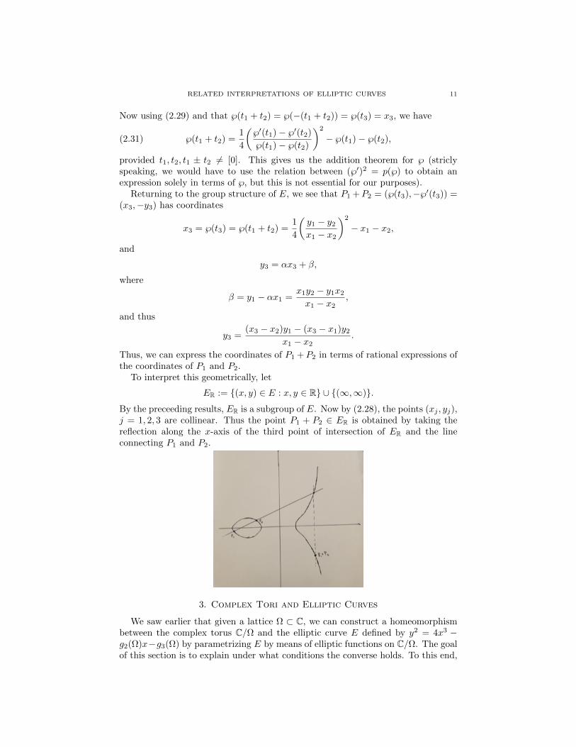
By the preceeding results, ER is a subgroup of E. Now by (2.28), the points (xj , yj),j = 1, 2, 3 are collinear. Thus the point P1 + P2 ∈ ER is obtained by taking thereflection along the x-axis of the third point of intersection of ER and the lineconnecting P1 and P2.

3. Complex Tori and Elliptic Curves

We saw earlier that given a lattice Ω ⊂ C, we can construct a homeomorphismbetween the complex torus C/Ω and the elliptic curve E defined by y2 = 4x3 −g2(Ω)x−g3(Ω) by parametrizing E by means of elliptic functions on C/Ω. The goalof this section is to explain under what conditions the converse holds. To this end,


we will employ some basic results from hyperbolic geometry; references [1] and [6]provide excellent treatments of this subject for the uninitiated reader.

3.1. Tori and Moduli. One of the difficulties we face in attempting to associatea torus to an elliptic curve is that there may be many tori that are homeomorphicto a given elliptic curve. If we can impose an equivalence relation on the set of allcomplex tori, then we are in a better position to investigate our question. But anytwo complex tori C/Ω and C/Ω′ are determined by their lattices Ω and Ω′, and soit suffices to impose an equivalence relation on the set of all lattices in C.

Definition 3.1. Two lattices Ω,Ω′ ⊂ C are said to be similar or homothetic ifthere exists some µ ∈ C \ 0 such that Ω′ = µΩ := µω : ω ∈ Ω.

It is not difficult to check that this is an equivalence relation. Furthermore, it is anon-trivial result that two complex tori C/Ω and C/Ω′ are conformally equivalent(meaning that they have the same complex analytic structures) if and only if Ωand Ω′ are similar (see Theorem 4.18.1 of [1]). Our present goal now becomes todetermine when two tori are similar; that is, we want to construct a function onthe set of all complex tori that takes on the same value at different tori if and onlyif the tori are similar.

By Lemma 2.4, if ω1, ω2 and ω′1, ω′2 are bases for Ω and Ω′ = µΩ, whereµ ∈ C \ 0, then there exist a, b, c, d ∈ Z with ad− bc = ±1 such that

ω′2 = µ(aω2 + bω1),

ω′1 = µ(cω2 + dω1).(3.2)

As ω1 and ω2 are linearly independent over R, we have Im (ω2/ω1) 6= 0. Inter-changing ω1 and ω2 if necessary, we can assume that Im (ω2/ω1) > 0. We nowdefine the modulus of the basis ω1, ω2 to be

τ =ω2

ω1,

where the numbering of the basis elements is chosen so that Im(τ) > 0. As eachlattice Ω has many bases, it determines a set of moduli. Since µω2/µω1 = ω2/ω1,similar lattices have the same set of moduli. Setting τ = ω2/ω1 and τ ′ = ω′2/ω

′1

(the moduli of the above bases for Ω and Ω′), we see from (3.2) that Ω and Ω′ aresimilar if and only if

τ ′ =aτ + b

cτ + d,(3.3)

where a, b, c, d ∈ Z and ad− bc = ±1. By the definition of the modulus of a basis,both τ and τ ′ lie in the upper half-plane H = z ∈ C : Im(z) > 0. Now ifad − bc = −1, then the Mobius transformation T : z 7→ (az + b)/(cz + d) maps Honto the lower half-plane, and we must therefore have ad − bc = 1. Conversely, ifa, b, c, d ∈ Z and ad− bc = 1, then from (3.2) we have a basis ω′1, ω′2 for a latticeΩ′ that is similar to Ω. Recall that the collection of all Mobius transformationsT : z 7→ (az + b)/(cz + d) with a, b, c, d ∈ Z and ad − bc = 1 forms the discretesubgroup PSL(2,Z) of PSL(2,R), which is called the modular group and which wewill denote by Γ. Our above argument has proved the following:

Theorem 3.4. If Ω = Ω(ω1, ω2) and Ω′ = Ω′(ω′1, ω′2) are lattices in C with moduli

τ = ω2/ω1 and τ ′ = ω′2/ω′1, then Ω and Ω′ are similar if and only if τ ′ = T (τ) for

some T ∈ Γ.


In other words, we can think of the equivalence classes of similar lattices ascorresponding to points of the quotient-space H/Γ.

3.2. The Modular Function. By Theorem 3.4, we have converted our problem ofdetermining when two lattices are similar to the problem of constructing a functionthat takes on the same value at two points τ, τ ′ ∈ H if and only if τ and τ ′ lie inthe some orbit of the action of Γ on H. Previously, we saw that the Weierstrass ℘function satisfies the differential equation ℘′ =

√p(℘), where p is a cubic polynomial

of the form

p(z) = 4z3 − c2z − c3 (c2, c3 ∈ C).(3.5)

A polynomial of the form (3.5) is said to be in Weierstrass normal form. Since anycubic polynomial can be brought in this form by means of a substitution of thetype φ : z 7→ az + b (a, b ∈ C, a 6= 0) and since φ : C → C is a bijection preservingthe multiplicities of roots, we will henceforth restrict our attention to polynomialsp in Weierstrass normal form. If e1, e2, and e3 are the roots of our polynomial p in(3.5), then we define the discriminant of p to be

∆p = 16(e1 − e2)2(e2 − e3)2(e1 − e3)2,

where we see that the ei are distinct if and only if ∆p 6= 0.3 Using the definitionof the discriminant and the relations between the roots of a polynomial and itscoefficients, it is relatively straightforward to see that ∆p = c32 − 27c23 (see section6.2 of [1], for example). As an immediate consequence, we deduce the following:

Corollary 3.6. The polynomial p(z) = 4z3− c2z− c3 has distinct roots if and onlyif c32 − 27c23 6= 0.

By Theorem 2.20, we know that the Weierstrass ℘ function associated to thelattice Ω satisfies ℘′(z) =

√p(℘), where p(z) = 4z3 − g2z − g3 and

g2 = g2(Ω) = 60∑

ω∈Ω\0

ω−4,

g3 = g3(Ω) = 140∑

ω∈Ω\0

ω−6.

If we let ∆(Ω) denote the discriminant ∆p of p, then by Theorem 2.24 and Corol-lary 3.6, we see that ∆(Ω) = g2(Ω)3 − 27g3(Ω)2 6= 0. Thus we may define themodular function J(Ω) by

J(Ω) =g2(Ω)3

∆(Ω)=

g2(Ω)3

g2(Ω)3 − 27g3(Ω)2.(3.7)

Now for a similar lattice µΩ (here µ 6= 0), we have

g2(µΩ) = 60∑

ω∈Ω\0

(µω)−4 = µ−4g2(Ω),

g3(µΩ) = 140∑

ω∈Ω\0

(µω)−6 = µ−6g3(Ω), and

∆(µΩ) = µ−12∆(Ω).

3This definition of the discriminant differs from how it is usually presented in texts on abstractalgebra; we have included the factor of 16 to conclude that ∆p = c32 − 27c23.


Therefore

J(µΩ) = J(Ω)(3.8)

for all µ ∈ C \ 0, showing that similar lattices determine the same value of J .In order to regard g2, g3,∆, and J as functions on the upper half-plane H, we

evaluate them at τ ∈ H by evaluating them on the lattice Ω(1, τ) that has τ as oneof its moduli. We then obtain

g2(τ) = 60∑

m,n∈Z\0

(m+ nτ)−4, and

g3(τ) = 140∑

m,n∈Z\0

(m+ nτ)−6.(3.9)

Additionally,

∆(τ) = g2(τ)3 − 27g3(τ)3,(3.10)

and

J(τ) =g2(τ)3

∆(τ).

Now if τ ′ = T (τ) for some T ∈ Γ, then by Theorem 3.4 the lattices Ω = Ω(1, τ)and Ω′ = Ω′(1, τ ′) are similar, and so (3.8) implies that J(Ω) = J(Ω′). This provesthe following:

Theorem 3.11. J(T (τ)) = J(τ) for all τ ∈ H and T ∈ Γ.

Thus J(τ) is invariant under the action of the modular group Γ. It will alsobe useful to understand how the action of Γ, as well as the orientation reversingtransformations of H, affect g2, g3, and ∆. Firstly, if T : τ 7→ (aτ + b)/(cτ + d) isan element of Γ, then

g2(T (τ)) = 60∑

m,n∈Z\0

(m+ n

(aτ + b)

(cτ + d)

)−4

= 60(cτ + d)−4∑

m,n∈Z\0

((md+ nb) + (mc+ na)τ)−4.

Since ad − bc = 1, Lemma 2.4 implies that the transformation (m,n) 7→ (md +nb,mc + na) simply permutes the elements of the set (m,n) ∈ Z × Z \ (0, 0).Then by the absolute convergence of our series (Theorem 2.13), we can rearrangethe elements to obtain

g2(T (τ)) = 60(cτ + d)−4∑

m,n∈Z\0

(m+ nτ)−4 = (cτ + d)−4g2(τ).(3.12)

We similarly find that

g3(T (τ)) = (cτ + d)−6g3(τ),(3.13)

and finally that

∆(T (τ)) = (cτ + d)−12∆(τ),(3.14)

from which we immediately deduce another proof of Theorem 3.11. In the particularcase when a = b = d = 1 and c = 0 so that T : τ 7→ τ + 1, we have the followingresult:


Theorem 3.15. The functions g2(τ), g3(τ), ∆(τ), and J(τ) are periodic withrespect to Z.

We will also need to understand how the above functions behave under the actionof the orientation reversing transformations of H, which are those of the form

T (τ) =aτ + b

cτ + d, (a, b, c, d ∈ Z, ad− bc = −1).(3.16)

Entirely analogous computations to those performed above show that

g2(T (τ)) = (cτ + d)−4g2(τ),

g3(T (τ)) = (cτ + d)−6g3(τ),

∆(T (τ)) = (cτ + d)−12∆(τ), and

J(T (τ)) = J(τ).

(3.17)

These formulas will soon play an important role in allowing us to show that Jprovides us with a surjection of the upper half-plane H onto the complex plane C.In particular, we will show that each c ∈ C is the pre-image under J of preciselyone orbit of the action of Γ on H. Before we can do this, we still need a bit moreinformation about g2(τ), g3(τ),∆(τ), and J(τ). The proofs of the following resultsare not conceptually difficult, but are rather long and technical; we now statethe results without proof, so as not to detract from the main idea of our currentexposition. For the proofs, see section 6.4 of [1].

Theorem 3.18. The functions g2, g3,∆, and J : H→ C are analytic on H.

Theorem 3.19. Let τ ∈ H and write q = e2πiτ so that 0 < |q| < 1. Then themodular function J : H→ C has a Laurent series expansion

J(τ) =1

1728

(1

q+

∞∑n=0

cnqn

),

where the cn are all integers.

3.3. The Lattice Associated to a Cubic. In this section, we achieve our aimof proving that if p(z) = 4z3 − c2z − c3 is a polynomial in the Weierstrass normalform (3.5) with distinct roots, then there exists a lattice Ω such that gk(Ω) = ckfor k = 2, 3. The key ingredient in this proof is the fact that J surjects H onto C.To prove this statement, we first need some more basic results.

Lemma 3.20. Let τ ∈ H.

(i) If 2Re(τ) ∈ Z, then g2(τ), g3(τ),∆(τ), and J(τ) are all real.

(ii) If |τ | = 1, then g2(τ) = τ4g2(τ), g3(τ) = τ6g3(τ), ∆(τ) = τ12∆(τ), and

J(τ) = J(τ).

Proof. The main idea of both parts is to use the hypotheses on τ to construct anorientation reversing transformation of H that fixes τ . In this way, the equations(3.17) give us relations between the images of τ under the functions g2, g3,∆, andJ , and the conjugates of these images, respectively.

(i) If 2 Re(τ) = n ∈ Z, then τ is fixed by the map T : τ → n− τ , which is of theform (3.16), with a = −1, b = n, c = 0, d = 1. The result is now immediate from(3.17).


(ii) If |τ | = 1, then τ is fixed by the map T : τ → 1/τ (geometrically, thismap represents the composition of an inversion with respect to the unit circle andreflection about the real axis). This map is again of the form (3.16), now witha = 0, b = 1, c = 1, and d = 0. Thus by (3.17), we obtain

g2(τ) = g2(1/τ) = (τ)−4g2(τ) = τ4g2(τ),

and similarly for the other functions.

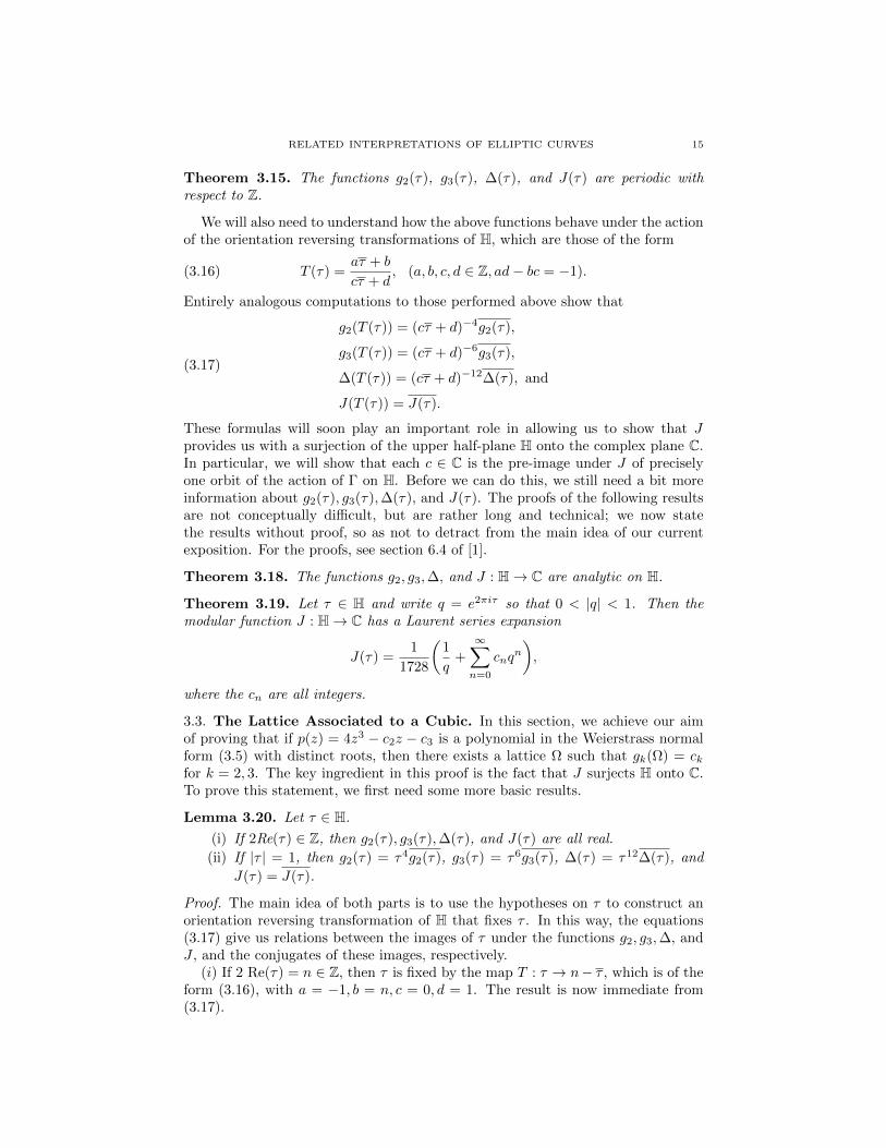
Recalling that the modular group Γ has as a fundamental region the set

F =

τ ∈ H : |τ | ≥ 1 and |Re(τ)| ≤ 1

2

,

the previous result allows us to immediately deduce the following.

Corollary 3.21. J(τ) is real whenever τ is on the imaginary axis or on the bound-ary ∂F of F .

Furthermore, Lemma 3.20 allows us to compute the value of J at certain specialpoints on ∂F .

Corollary 3.22. Let ρ = e2πi/3. Then g2(ρ) = g3(i) = J(ρ) = 0 and J(i) = 1.

Proof. Part (i) of Lemma 3.20 shows that g2 and g3 both take on real values at thepoints i and ρ. This along with part (ii) of the lemma shows that g2(ρ) = ρg2(ρ)and g3(i) = −g3(i). Therefore, g2(ρ) = g3(i) = 0, and by the formula for J we alsoobtain J(ρ) = 0 and J(i) = 1.

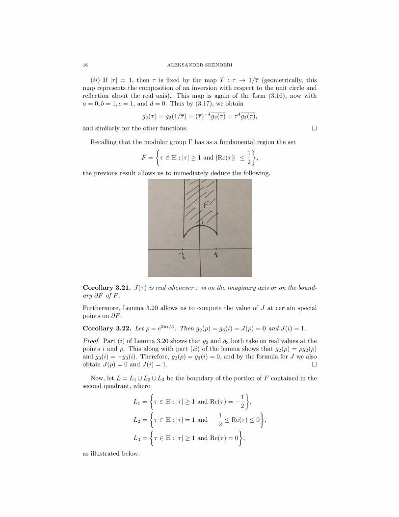
Now, let L = L1 ∪L2 ∪L3 be the boundary of the portion of F contained in thesecond quadrant, where

L1 =

τ ∈ H : |τ | ≥ 1 and Re(τ) = −1

2

,

L2 =

τ ∈ H : |τ | = 1 and − 1

2≤ Re(τ) ≤ 0

,

L3 =

τ ∈ H : |τ | ≥ 1 and Re(τ) = 0

,

as illustrated below.


By Corollary 3.21, we know that J(L) ⊂ R. We now show that the reverse inclusionalso holds.

Theorem 3.23. The modular function J maps the set L onto R.

Proof. The main idea is to use the Laurent series expansion of J given in Theorem3.19 to deduce some topological information about the image set J(L). The factthat J is analytic on H, which is guaranteed by Theorem 3.18, will then forceJ(L) = R.

If τ ∈ L3, then we have τ = iy for y ≥ 1. Hence q = e2πiτ = e−2πy, and asy →∞, we have q → 0, through positive real values. Since

J(τ) =1

1728

(1

q+

∞∑n=0

cnqn

).

we have J(τ)→∞ as q → 0. Similarly if τ ∈ L1, then τ = −1/2 + iy, where y ≥ 1,and therefore q = −e−2πy. Thus as y → ∞, we have q → 0 through negative realvalues, and therefore J(τ)→ −∞. This shows that as a real-valued function on L(Corollary 3.21), J is unbounded from above and below. But Theorem 3.18 tellsus that J is analytic on H, and so, in particular, J is continuous on H; since L isconnected, it follows that J(L) is connected. But any connected subset of R thatis unbounded from above and below must be R itself, and thus J(L) = R.

Notice that if we did not include the set L2 in the definition of L, but simplydefined L = L1 ∪L3, then the above argument would not work, since L would thennot be connected.

The following result is the culmination of our studies of the J function and willplay a crucial role in proving the main theorem of this section.

Theorem 3.24. For each c ∈ C, there is exactly one orbit of Γ in H on which Jtakes the value c.

Proof. By the definition of a fundamental region for a Fuchsian group, we knowthat each orbit of Γ meets F at either a unique point in the interior F o of F , or atone or two equivalent points on ∂F .

Suppose first that c ∈ C \ R. By Corollary 3.21 we have J(∂F ) ⊂ R (moreprecisely, by using Theorem 3.23, we have J(∂F ) = R) and so it suffices to showthat there is precisely one solution of J(τ) = c in F o. The idea is to express


the number of solutions of the equation J(τ) = c as the number of residues of anappropriate function, so that we may use Cauchy’s Residue Theorem (a similarstrategy was employed earlier in the proof of Theorem 2.12). By Theorem 3.18 andCorollary 3.22, we know that J is analytic and not identically equal to c, and sothe function

g(τ) =J ′(τ)

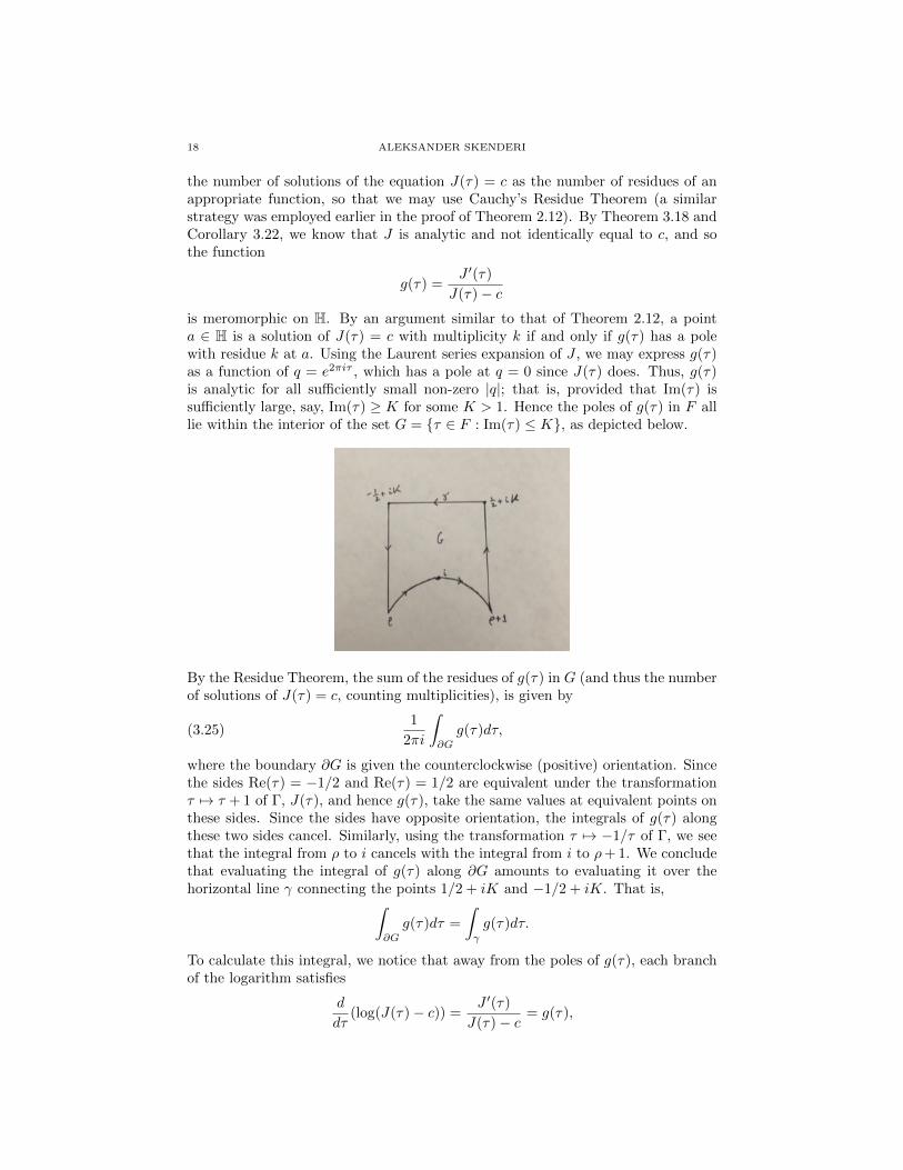
J(τ)− cis meromorphic on H. By an argument similar to that of Theorem 2.12, a pointa ∈ H is a solution of J(τ) = c with multiplicity k if and only if g(τ) has a polewith residue k at a. Using the Laurent series expansion of J , we may express g(τ)as a function of q = e2πiτ , which has a pole at q = 0 since J(τ) does. Thus, g(τ)is analytic for all sufficiently small non-zero |q|; that is, provided that Im(τ) issufficiently large, say, Im(τ) ≥ K for some K > 1. Hence the poles of g(τ) in F alllie within the interior of the set G = τ ∈ F : Im(τ) ≤ K, as depicted below.

By the Residue Theorem, the sum of the residues of g(τ) in G (and thus the numberof solutions of J(τ) = c, counting multiplicities), is given by

1

2πi

∫∂G

g(τ)dτ,(3.25)

where the boundary ∂G is given the counterclockwise (positive) orientation. Sincethe sides Re(τ) = −1/2 and Re(τ) = 1/2 are equivalent under the transformationτ 7→ τ + 1 of Γ, J(τ), and hence g(τ), take the same values at equivalent points onthese sides. Since the sides have opposite orientation, the integrals of g(τ) alongthese two sides cancel. Similarly, using the transformation τ 7→ −1/τ of Γ, we seethat the integral from ρ to i cancels with the integral from i to ρ+ 1. We concludethat evaluating the integral of g(τ) along ∂G amounts to evaluating it over thehorizontal line γ connecting the points 1/2 + iK and −1/2 + iK. That is,∫

∂G

g(τ)dτ =

∫γ

g(τ)dτ.

To calculate this integral, we notice that away from the poles of g(τ), each branchof the logarithm satisfies

d

dτ(log(J(τ)− c)) =

J ′(τ)

J(τ)− c= g(τ),


and so ∫γ

g(τ)dτ = log(J(τ)− c)∣∣γ,

where the change in the value of log(J(τ) − c) arises from analytic continuationalong γ. Indeed, as τ follows γ, the point q winds once (in the clockwise, negativedirection) around the circle C given by |q| = e−2πk, beginning and finishing at−e−2πK . By Theorem 3.19, q(J(τ) − c) is analytic and non-zero for all 0 ≤ |q| ≤e−2πK . Since this set is simply connected, the monodromy theorem implies that

log(q(J(τ)− c))∣∣γ

= 0,

and therefore

log(J(τ)− c)∣∣γ

=[log(q(J(τ)− c))− logq

]γ

= [−log(q)]γ = 2πi.

By (3.25), we have that the number of solutions of J(τ) = c in F is equal to 1, asrequired.

Finally suppose that c ∈ R. By Theorem 3.23, there is at least one orbit of Γ onwhich J takes the value c. If there were two such orbits, then there would exist twonon-equivalent solutions τ1 and τ2 of the equation J(τ) = c. By choosing c′ ∈ C\Rsufficiently close to c, we would obtain two non-equivalent solutions to the equationJ(τ) = c′. But we have already shown that this is impossible; hence τ1 and τ2 mustbe in the same orbit of Γ, and thus the orbit is unique.

We are finally able to prove the converse to Theorem 2.25.

Theorem 3.26. If c2, c3 ∈ C satisfy c32 − 27c23 6= 0, then there is a lattice Ω ⊂ Cwith gk(Ω) = ck, for k = 2, 3. That is, if p(z) = 4z3 − c2z − c3, where c2 and c3are as above, then the elliptic curve y2 = p(z) is homeomorphic to C/Ω for somelattice Ω.

Proof. There are three separate cases to consider. Suppose first that c2 = 0. Thenby hypothesis, c3 6= 0. By Corollary 3.22, we know that g2(ρ) = 0, and since∆(τ) = g2(τ)3 − 27g3(τ)2 never vanishes on H, we conclude that g3(ρ) 6= 0. Thusthere exists some µ ∈ C \ 0 such that µ−6g3(ρ) = c3. So, if we set

Ω = µΩ(1, ρ) = Ω(µ, µρ),

then we have g2(Ω) = µ−4g2(ρ) = 0 = c2, and g3(Ω) = µ−6g3(ρ) = c3, as required.Suppose now that c3 = 0, so that c2 6= 0. By Corollary 3.22, g3(i) = 0, and so

similarly to as before, we must have g2(i) 6= 0. Hence, there exists µ ∈ C \ 0 suchthat µ−4g2(i) = c2. Setting

Ω = µΩ(1, i) = Ω(µ, µi),

we find that g2(Ω) = µ−4g2(i) = c2, and g3(Ω) = µ−6g3(i) = 0 = c3, as desired.We now consider the general case when c2, c3 6= 0. By Theorem 3.24, there exists

some τ ∈ H such that

g2(τ)3

g2(τ)3 − 27g3(τ)2= J(τ) =

c32c32 − 27c23

.

As c2 6= 0, we have g2(τ) 6= 0. We also see that g3(τ) 6= 0, since if g3(τ) = 0,then J(τ) = 1, and hence c3 = 0, a contradiction. Thus after some algebraic


manipulations, we obtain the well-defined equality of non-zero complex numbers

c32g2(τ)3

=c23

g3(τ)2.(3.27)

There exists some µ ∈ C \ 0 such that µ−4 = c2/g2(τ). By (3.27), we obtain

µ−12 =c32

g2(τ)3=

c23g3(τ)2

, and so,

µ−6 = ± c3g3(τ)

.

Replacing µ by iµ if necessary, we have µ−4 = c2/g2(τ) and µ−6 = c3/g3(τ). Thus

Ω = µΩ(1, τ) = Ω(µ, µτ)

is our desired lattice. The second statement of the theorem is immediate fromTheorem 2.25.

As a final remark, we note that it is actually possible to prove a stronger result.Namely, if p(z) is a polynomial with distinct roots (so that is can be put in theWeierstrass normal form 4z3 − c2z − c3, with c32 − 27c23 6= 0), then the Riemann

surface of w =√p(z) is in fact conformally equivalent to C/Ω for some lattice

Ω ⊂ C (see Theorem 6.5.11 of [1]). As we remarked below Definition 3.1, twotori C/Ω and C/Ω′ are conformally equivalent if and only if they are similar. ByTheorem 3.4, this occurs if and only if their moduli τ and τ ′ are in the same orbit ofΓ on H. Thus the points of the quotient space H/Γ represent the set of all complexstructures that may be placed on an elliptic curve, yielding yet another beautifulresult concerning elliptic curves over C.

Acknowledgments

I would like to thank Professor Matthew Emerton for meeting with me manytimes throughout the summer to teach me about elliptic curves; my knowledge ofthe subject was greatly enriched by having the opportunity to learn from him. Iwould also like to thank Thomas Hameister for the many helpful discussions wehad about elliptic curves and algebraic geometry, and for his reading this paperand providing me with very useful feedback. Additionally, I thank Yuchen Chenand Ethan Schondorf for the several discussions we had about this subject. Lastbut certainly not least, I would like to thank Professor Peter May for the efforthe puts into organizing the UChicago REU, and for giving me the opportunity toparticipate in it.

References

[1] Jones, G.A. and Singerman, D Complex Functions: An algebraic and geometric viewpoint

Cambridge University Press, Cambridge, 1987.

[2] Shafarevich, I. Basic Algebraic Geometry I: Varieties in Projective SpaceSpringer-Verlag, 2013.

[3] Silverman, Joseph H. The Arithmetic of Elliptic Curves

Springer, 2009.[4] Reid, Miles. Undergraduate Algebraic Geometry

Cambridge University Press, 1988.[5] Shurman, Jerry. Complex Tori as Elliptic Curves

https : //people.reed.edu/ jerry/311/toriec.pdf


[6] Fraser, Jonathan M. MT 5830: Topics in Geometry and Analysis

http : //www.mcs.st− andrews.ac.uk/ jmf32/teaching.html 2017.

RELATED INTERPRETATIONS OF ELLIPTIC CURVES

Documents

Transcript of RELATED INTERPRETATIONS OF ELLIPTIC CURVES