Introduction To Elliptic Curves - uni-heidelberg.dehb3/publ/pseoul.pdfThe torsion subgroup of...
51
Introduction To Elliptic Curves Franz Lemmermeyer August 9, 2011
Transcript of Introduction To Elliptic Curves - uni-heidelberg.dehb3/publ/pseoul.pdfThe torsion subgroup of...
Introduction To Elliptic Curves
Franz Lemmermeyer
August 9, 2011
2
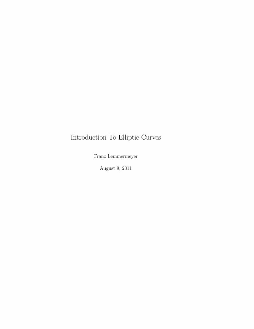
These are the notes for some lectures on the arithmetic of elliptic curvesgiven in Seoul in August 2002.
Lecture 1 Aug. 08, 2002
Lecture 2 Aug. 09, 2002
Lecture 3 Aug. 12, 2002
Lecture 4 Aug. 13, 2002
Lecture 5 Aug. 14, 2002
Contents
1. The Rank of Elliptic Curves 51.1 Introduction . . . . . . . . . . . . . . . . . . . . . . . . . . . . . . 51.2 Rational Points on Elliptic Curves . . . . . . . . . . . . . . . . . 61.3 Simple 2-descent . . . . . . . . . . . . . . . . . . . . . . . . . . . 81.4 Tate’s Method . . . . . . . . . . . . . . . . . . . . . . . . . . . . 11
2. Local Solvability 132.1 Example . . . . . . . . . . . . . . . . . . . . . . . . . . . . . . . . 132.2 Quartics over Fp . . . . . . . . . . . . . . . . . . . . . . . . . . . 142.3 Reichardt’s Counterexample to the Hasse Principle . . . . . . . . 17
3. Conics 193.1 Parametrization . . . . . . . . . . . . . . . . . . . . . . . . . . . . 193.2 The Group Law . . . . . . . . . . . . . . . . . . . . . . . . . . . . 193.3 The Group Structure . . . . . . . . . . . . . . . . . . . . . . . . . 213.4 Computing the Rank . . . . . . . . . . . . . . . . . . . . . . . . . 23
4. 2-Descent (Proofs) 294.1 2-Isogenies . . . . . . . . . . . . . . . . . . . . . . . . . . . . . . . 294.2 The Snake Lemma . . . . . . . . . . . . . . . . . . . . . . . . . . 324.3 Tate’s formula . . . . . . . . . . . . . . . . . . . . . . . . . . . . 334.4 Heights . . . . . . . . . . . . . . . . . . . . . . . . . . . . . . . . 344.5 Selmer and Tate-Shafarevich Groups . . . . . . . . . . . . . . . . 35
5. Nontrivial Elements in qq[2] 375.1 Pepin’s Claims . . . . . . . . . . . . . . . . . . . . . . . . . . . . 375.2 Applications of Genus Theory . . . . . . . . . . . . . . . . . . . . 375.3 Using 2-descent . . . . . . . . . . . . . . . . . . . . . . . . . . . . 39
6. 3-Descent 436.1 3-Descent on Curves with Rational 3-Torsion . . . . . . . . . . . 436.2 The 3-Isogenous Curve . . . . . . . . . . . . . . . . . . . . . . . . 456.3 The Rank Formula . . . . . . . . . . . . . . . . . . . . . . . . . . 476.4 The Image of α and β . . . . . . . . . . . . . . . . . . . . . . . . 49
3

4
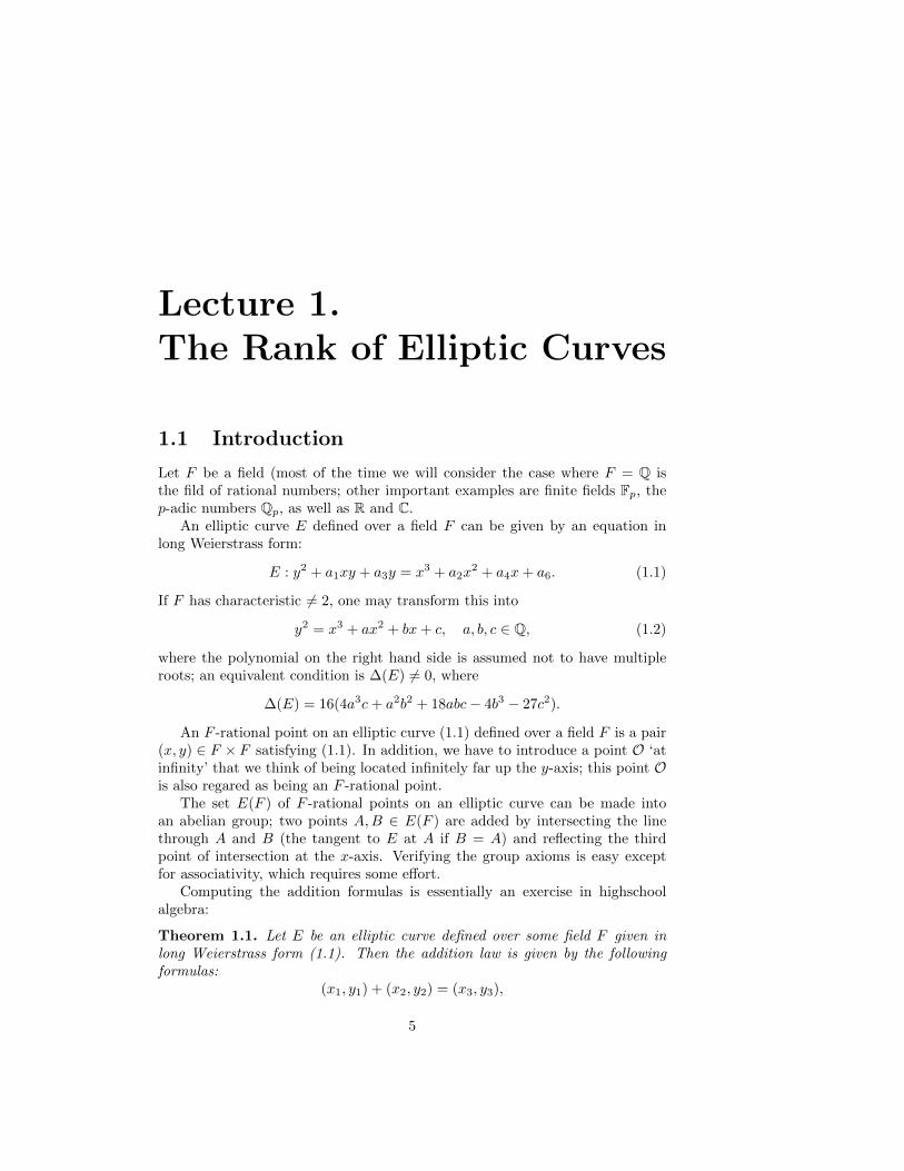
Lecture 1.The Rank of Elliptic Curves
1.1 Introduction
Let F be a field (most of the time we will consider the case where F = Q isthe fild of rational numbers; other important examples are finite fields Fp, thep-adic numbers Qp, as well as R and C.
An elliptic curve E defined over a field F can be given by an equation inlong Weierstrass form:
E : y2 + a1xy + a3y = x3 + a2x2 + a4x+ a6. (1.1)
If F has characteristic 6= 2, one may transform this into
y2 = x3 + ax2 + bx+ c, a, b, c ∈ Q, (1.2)
where the polynomial on the right hand side is assumed not to have multipleroots; an equivalent condition is ∆(E) 6= 0, where
∆(E) = 16(4a3c+ a2b2 + 18abc− 4b3 − 27c2).
An F -rational point on an elliptic curve (1.1) defined over a field F is a pair(x, y) ∈ F × F satisfying (1.1). In addition, we have to introduce a point O ‘atinfinity’ that we think of being located infinitely far up the y-axis; this point Ois also regared as being an F -rational point.
The set E(F ) of F -rational points on an elliptic curve can be made intoan abelian group; two points A,B ∈ E(F ) are added by intersecting the linethrough A and B (the tangent to E at A if B = A) and reflecting the thirdpoint of intersection at the x-axis. Verifying the group axioms is easy exceptfor associativity, which requires some effort.
Computing the addition formulas is essentially an exercise in highschoolalgebra:
Theorem 1.1. Let E be an elliptic curve defined over some field F given inlong Weierstrass form (1.1). Then the addition law is given by the followingformulas:
(x1, y1) + (x2, y2) = (x3, y3),
5
6 Franz Lemmermeyer 1. The Rank of Elliptic Curves
where
x3 = −x1 − x2 − a2 + a1m+m2
y3 = −y1 − (x3 − x1)m− a1x3 − a3
and
m =
y2 − y1x2 − x1
if x1 6= x2
3x21 + 2a2x1 + a4 − a1y12y1 + a1x1 + a3
if x1 = x2
1.2 Rational Points on Elliptic Curves
The structure of the abelian group E(Q) is described by the following theorem:
Theorem 1.2 (Mordell-Weil). The group E(Q) is finitely generated. In partic-ular,
E(Q) = E(Q)tors ⊕ Zr,
where E(Q)tors is a finite group, and where r ≥ 0 is a non-negative integer calledthe Mordell-Weil rank of E.
Theorem 1.2 was first proved by Mordell in the 1920s; as Weil has shownin 1928, it holds with Q replaced by any number field, and even with ellipticcurves replaced by abelian varieties. Observe the analogy with number fields K:the units UK of K form a finitely generated abelian group, and by Dirichlet’sunit theorem we have
UK ' (UK)tors ⊕ Zr,
where (UK)tors is the group of roots of unity in K, and where r is the unit rank,which can be computed in terms of the number of real and complex embeddingsof K. For elliptic curves, determining r is a much more difficult problem.
The proof of the Mordell-Weil Theorem consists of two parts. The algebraicpart is called the Weak Mordell-Weil Theorem:
Theorem 1.3. Given an elliptic curve E defined over Q, there is an integerm > 1 such that E(Q)/mE(Q) is finite.
Actually, this is true for any integer m > 1, but one such m is sufficient forthe proof. The simplest proofs use m = 2.
For showing that E(Q) is finitely generated we need a second ingredient:heights. These are machines that measure how complicated rational pointsare. We first define the height H(x) of rational numbers x ∈ Q by writingx = m
n with gcd(m,n) = 1 and then putting H(x) = max{|m|, |n|}. Note thatH(0) = H( 0
1 ) = 1. Observe that there are only finitely many rational numbersof height < C for any fixed constant C > 0.
Rational Points on Elliptic Curves 7
For a rational point P ∈ E(Q) on an elliptic curve E we can now put
h(P ) =
{1 if P = O,logH(x) if P = (x, y).
Again it is easy to see that on a given elliptic curve E there are only finitelypoints of height bounded by some constant C > 0.
The second part of the proof of the Mordell-Weil theorem consists in checkingthat the height defined above is ‘compatible’ with the group law in the sensethat one can bound h(P +Q) in terms of h(P ) and h(Q).
The torsion part of E(Q) is rather easy to compute:
Theorem 1.4 (Nagell-Lutz). Let E : y2 = x3 + ax+ b be an elliptic curve witha, b ∈ Z. If P = (x, y) ∈ E(Q) is a torsion point, theni) x, y ∈ Z;ii) y = 0 or y2 | D = 4a3 + 27b2.
As an example, consider the curve E : y2 = x3 + 1. Here D = 27, so if(x, y) ∈ E(Q)tors, then y = 0 or y2 | 27. By going through all these cases wefind the following candidates of torsion points: O, (−1, 0), (0,±1), (2,±3). Weclaim that these are in fact torsion; for a proof it is sufficient to show that theyare all killed by 6.
In fact, using the addition formulas we easily show that
2 · (2, 3) = (0, 1),
3 · (2, 3) = (0, 1) + (2, 3) = (−1, 0),
4 · (2, 3) = 2 · (0, 1) = (0,−1),
5 · (2, 3) = (0, 1) + (−1, 0) = (2,−3),
6 · (2, 3) = 2 · (−1, 0) = O.
Thus E(Q)tors ' Z/6Z.
For elliptic curves in short Weierstrass form (1.2), torsion points of order 2can be described explicitly: if x1, x2, x3 ∈ C denote the roots of the polynomialx3 + ax2 + bx+ c, then
E(Q)[2] = {O, (x1, 0), (x2, 0), (x3, 0)}.
Thus E has a rational point of order 2 if and only if x3 + ax2 + bx + c has arational root.
The torsion subgroup of elliptic curves defined over Q can be computed usingpari. Elliptic curves are described by the long Weierstraß equation
y2 + a1xy + a3y = x3 + a2x2 + a4x+ a6
(for memorizing, give x weight 2, y weight 3, and ak weight k; then each termhas weight 6), so our curve has a1 = a2 = a3 = a4 = 0, a6 = 1, and we initialize
8 Franz Lemmermeyer 1. The Rank of Elliptic Curves
by typing e = ellinit([0,0,0,0,1]). Then elltors(e) produces the output[6, [6], [[2,3]]]: the first number is the cardinality of E(Q)tors, the secondterm [6] symbolizes the abstract structure Z/6Z of E(Q)tors, and [2, 3] is a pointgenerating the torsion subgroup.
The following deep result describes all possible torsion groups of ellipticcurves over Q:
Theorem 1.5 (Mazur). Let E be an elliptic curve defined over Q. ThenE(Q)tors is isomorphic to one of the following 15 groups:
E(Q)tors '
Z/2Z× Z/2mZ fur 1 ≤ m ≤ 4;
Z/(2m− 1)Z fur 1 ≤ m ≤ 5;
Z/2mZ fur 1 ≤ m ≤ 6.
(1.3)
Loic Merel recently proved that the cardinality of E(K)tors of elliptic curvesover number fields K can be bounded in terms of the degree (K : Q).
1.3 Simple 2-descent
In this section we are interested in studying rational points on cubic curves ofthe form
E : y2 = x3 + ax2 + bx+ c, (1.4)
where a, b, c are assumed to be integers. The rational points on (1.4) have avery special form:
Lemma 1.6. Let P = (x, y) be a rational point on (1.4); then there existm,n, e ∈ Z such that x = m/e2, y = n/e3, and (m, e) = (n, e) = 1.
Proof. Write x = m/M und y = n/N with m,n ∈ Z, M,N ∈ N and (m,M) =(n,N) = 1. We want to show that M3 | N2 and N2 | M3, since this impliesM3 = N2, that is, M = e2 and N = e3 for some e ∈ N (here we are using uniquefactorization: N2 = M3 implies that the exponent with which each prime factorappears is divisible by 2 and 3, hence by 6).
From y2 = x3 + ax2 + bx+ c we get
M3n2 = N2m3 + aN2Mm2 + bN2M2m+ cN2M3.
Since the right hand side is divisible by N2, and since we know that (n,N) =1, we conclude that N2 | M3. On the other hand we have M | N2m3 and(m,M) = 1, hence M | N2. This implies M2 | N2m3, that is, M | N , andrunning through this argument once more we find M3 | N2.
From now on we consider curves (1.4) with c = 0:
y2 = x(x2 + ax+ b), a, b ∈ Z, b(a2 − 4b) 6= 0. (1.5)
Simple 2-descent 9
These curves have the rational point T = (0, 0); since 2T = O, this is a torsionpoint of order 2.
Now let us take such a rational point P = (x, y) on such a curve (1.5) withx = m/e2 and y = n/e3 as in Lemma 1.6. Plugging this into equation (1.5) weget
n2 = m(m2 + ame2 + be4).
Thus we have two integers whose product is a square; if these integers werecoprime we could conclude that each of them is a square since the integers form aUFD. Let us compute a bit: gcd(m,m2+ame2+be4) = gcd(m, be4) = gcd(m, b),since (m, e) = 1 by Lemma 1.6. If we write b1 = gcd(m, b), then b = b1b2 andm = b1u. This gives
n2 = b1u(b21u2 + ab1ue
2 + b1b2e4),
and with n = b1z we get
z2 = u(b1u2 + aue2 + b2e
4).
Let us assume for now that n 6= 0. The two factors now are coprime (wejust divided through by the greatest common divisor), and we see that u mustbe a square up to a unit factor. But by choosing the sign of b1 appropriately wemay assume that u = M2 and b1u
2 + aue2 + b2e4 = N2 for integers M,N ∈ N
with MN = z. Replacing u by M2 in the second equation we finally get
T (ψ)(b1) : N2 = b1M4 + aM2e2 + b2e
4. (1.6)
Thus every point (x, y) ∈ E(Q) gives rise to a point (N,M, e) on the curveT (ψ)(b1), where b1 is given by b1 = gcd(m, b) and x = m
e2 . Conversely, given
(N,M, e) on T (ψ)(b1), we can get back our point (x, y) by reversing the con-struction. We know that MN = z and n = b1z; moreover M2 = u and b1u = m.Thus (x, y) = (b1(M/e)2, b1NM/e3). In particular, b1 and x differ only by asquare factor. This is a surprising result: if (x, y) ∈ E(Q), then even if E(Q) isinfinite, there are only finitely many b1 such that x/b1 is a square.
Before we explore this further, let us address the case n = 0. If m = 0, then(x, y) = (0, 0), hence b1 = gcd(m, b) = b, and in fact N2 = bM4+aM2e2+e4 hasthe solution (N,M, e) = (1, 0, 1) giving rise to the point (0, 0) ∈ E(Q). Assumenow that m 6= 0. Then (x, 0) must be a rational 2-torsion point different from(0, 0); since torsion points have integral coordinates, we have P = (c, 0) andQ = (d, 0) for integers c, d; in particular we have e = 1. From x2 + ax + b =(x−c)(x−d) we read off a = −c−d and b = cd, so for P we get b1 = gcd(m, b) =gcd(c, cd) = c, and similarly b1 = d for Q. Thus in these cases, b1 is given bythe x-coordinate of the point.
We have shown that every rational point on (1.5) corresponds to a non-trivial1 primitive2 integral solution of one of the finitely many3 curves (1.6);
1That is, we do not count the solution N = M = e = 0.2This is our abbreviation for (N, e) = (M, e) = 1.3There are only finitely many divisors b1 of b.
10 Franz Lemmermeyer 1. The Rank of Elliptic Curves
these curves are called torsors of the elliptic curve (1.5) and will be denoted byT (ψ)(b1) in the following (the superscript (ψ) will be explained below). Torsorswith a rational point are called trivial. By reversing our construction we alreadyhave seen that every integral point on (1.6) yields a rational point on (1.5): infact, if (N,M, e) is a solution of (1.6), then P = (x, y) is a rational point on (1.5),where x = b1M
2/e2 and y = b1MN/e3; solutions with e = 0 correspond to therational point O at infinity. Such a solution occurs if and only if N2 = b1M
4,that is, if and only if b1 is a square.
We also see that the solvability of (1.6) only depends on b1 modulo squares:in fact, if (N,M, e) solves the torsor T (ψ)(b1), then (fN,M, fe) solves the torsorT (ψ)(b1f
2). Thus we only need to look at squarefree values of b1:
Theorem 1.7. The rational points on the elliptic curve (1.5) are in bijectionwith non-trivial primitive integral solutions on the torsors (1.6), where b1 runsthrough the squarefree divisors of b = b1b2.
Given (N,M, e) on T (ψ)(b1), the point (x, y) = (b1M2/e2, b1MN/e3) is a
rational point on E(Q). Conversely, P = (x, y) ∈ E(Q) gives a primitive integralsolution (N,M, e) on the torsor T (ψ)(b1), where b1 is the squarefree numberdetermined by α(P ) = b1Q× 2, where α : E(Q) −→ Q×/Q× 2 is the map givenby
α(P ) =
1Q× 2 if P = O;
bQ× 2 if P = (0, 0);
xQ× 2 if P = (x, y) ∈ E(Q) \ {O, (0, 0)}.(1.7)
Observe that if (N,M, e) is a rational point on some torsor, and if d is theproduct of the denominators of N , M and e, then (d2N, dM, de) is a point onthe torsor with integral coordinates, and this point gives rise to the same pointon E as (N,M, e).
Remark. Note that in our proof we have shown that gcd(N,M) = 1; wedid, however, not assume that b1 is squarefree. Thus we may assume thatgcd(N,M) = 1 as long as b1 runs through all divisors of b. If we restrict thevalues of b1 to the squarefree divisors of b, then we have to allow commondivisors of N and M . In any case we may assume that (N, e) = (M, e) = 1: acommon prime divisor of N and e divides M since b1 is squarefree, and we maycancel the fourth power of the common divisor; similarly we can ensure that(M, e) = 1.
We shall call α : E(Q) −→ Q×/Q× 2 the Weil map (it was introduced byAndre Weil in his proof of Mordell’s theorem). We found the Weil map from thegroup of rational points on E to the group Q×/Q× 2 by studying the rationalpoints on elliptic curves (1.6). Later we shall prove that this map is actually agroup homomorphism; here we stayed away from everything involving the grouplaw on elliptic curves and only used ‘classical’ methods, namely nothing beyondunique factorization.
Tate’s Method 11
1.4 Tate’s Method
In this section we want to describe Tate’s method for computing the rank of(certain) elliptic curves E : y2 = x(x2 + ax + b). The idea is to consider E
simultaneously with the 2-isogenous curve E : y2 = x(x2 + a x + b ), where
a = −2a and b = a2 − 4b. Here’s what to do:
1. List all torsors T (ψ)(b1) : N2 = b1M4 + aM2e2 + b2e
4, where b1 runsthrough the squarefree divisors of b = b1b2; the number of such torsorsthat have a rational point 6= (0, 0, 0) is a power of 2, say 2w.
2. List all torsors T (φ)(b1) : N2 = b1M4 + aM2e2 + b2e
4, where b1 runs
through the squarefree divisors of b = b1b2; the number of such torsorsthat have a rational point 6= (0, 0, 0) is a power of 2, say 2w .
3. The rank of E (and of E) is given by r = w + w − 2.
Example. 1. Consider E : y2 = x(x2 + 1). There are only two squarefreedivisors of b = 1, but only T (ψ)(1) has a rational point:
b1 T (ψ)(b1) (N,M, e) P
1 N2 = M4 + e4 (1, 1, 0) O
− 1 N2 = −M4 − 5e4
Thus w = 0.2. Consider E : y2 = x(x2 − 4). Here we find four torsors:
b1 T (φ)(b1) (N,M, e) P
1 N2 = M4 − 4e4 (1, 1, 0) O
− 1 N2 = −4M4 + e4 (1, 0, 1) (0, 0)
2 N2 = 2M4 − 2e4 (0, 1, 1) (2, 0)
− 2 N2 = −2M4 + 2e4 (0, 1, 1) (−2, 0)
Thus w = 2.3. Now Tate’s formula gives r = 0 + 2−2 = 0, that is, E(Q) = E(Q)tors and
E(Q) = E(Q)tors. Determining these torsion groups using Nagell-Lutz is left asan exercise.
As we will see, the main problem with this method is that we do not havean algorithm for deciding which of the torsors T (b1) have rational points andwhich don’t.
12 Franz Lemmermeyer 1. The Rank of Elliptic Curves
Lecture 2.Local Solvability
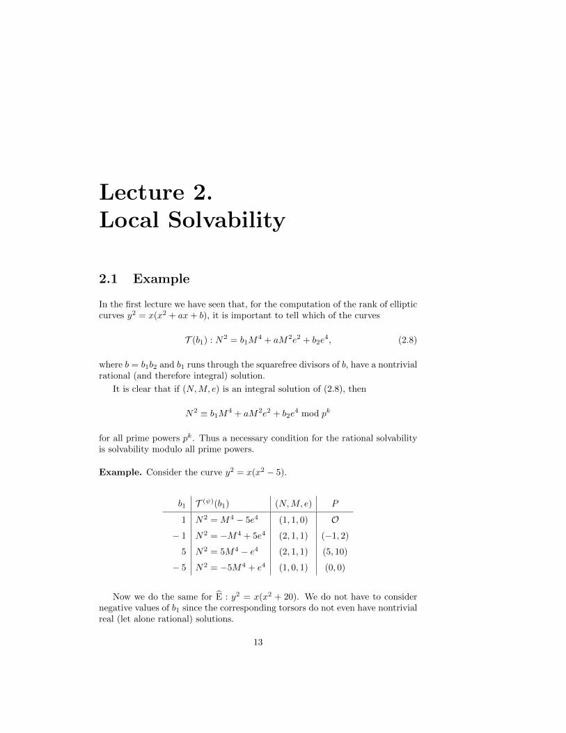
2.1 Example
In the first lecture we have seen that, for the computation of the rank of ellipticcurves y2 = x(x2 + ax+ b), it is important to tell which of the curves
T (b1) : N2 = b1M4 + aM2e2 + b2e
4, (2.8)
where b = b1b2 and b1 runs through the squarefree divisors of b, have a nontrivialrational (and therefore integral) solution.
It is clear that if (N,M, e) is an integral solution of (2.8), then
N2 ≡ b1M4 + aM2e2 + b2e4 mod pk
for all prime powers pk. Thus a necessary condition for the rational solvabilityis solvability modulo all prime powers.
Example. Consider the curve y2 = x(x2 − 5).
b1 T (ψ)(b1) (N,M, e) P
1 N2 = M4 − 5e4 (1, 1, 0) O
− 1 N2 = −M4 + 5e4 (2, 1, 1) (−1, 2)
5 N2 = 5M4 − e4 (2, 1, 1) (5, 10)
− 5 N2 = −5M4 + e4 (1, 0, 1) (0, 0)
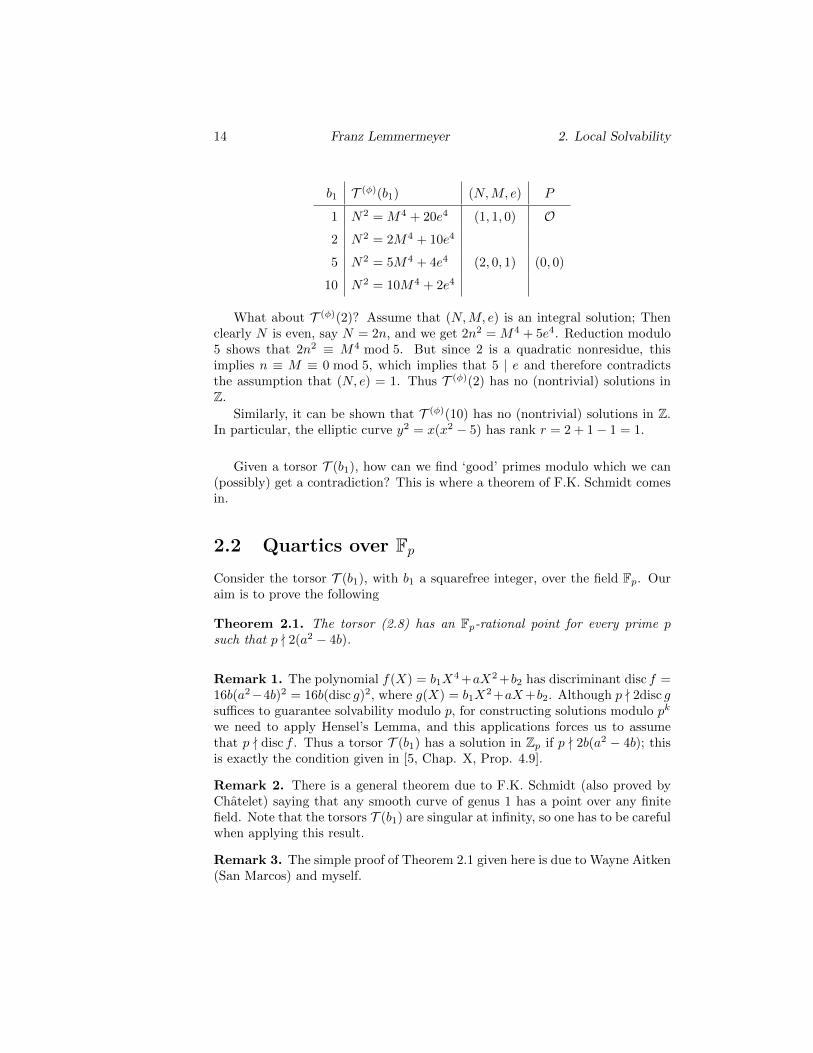
Now we do the same for E : y2 = x(x2 + 20). We do not have to considernegative values of b1 since the corresponding torsors do not even have nontrivialreal (let alone rational) solutions.
13
14 Franz Lemmermeyer 2. Local Solvability
b1 T (φ)(b1) (N,M, e) P
1 N2 = M4 + 20e4 (1, 1, 0) O
2 N2 = 2M4 + 10e4
5 N2 = 5M4 + 4e4 (2, 0, 1) (0, 0)
10 N2 = 10M4 + 2e4
What about T (φ)(2)? Assume that (N,M, e) is an integral solution; Thenclearly N is even, say N = 2n, and we get 2n2 = M4 + 5e4. Reduction modulo5 shows that 2n2 ≡ M4 mod 5. But since 2 is a quadratic nonresidue, thisimplies n ≡ M ≡ 0 mod 5, which implies that 5 | e and therefore contradictsthe assumption that (N, e) = 1. Thus T (φ)(2) has no (nontrivial) solutions inZ.
Similarly, it can be shown that T (φ)(10) has no (nontrivial) solutions in Z.In particular, the elliptic curve y2 = x(x2 − 5) has rank r = 2 + 1− 1 = 1.
Given a torsor T (b1), how can we find ‘good’ primes modulo which we can(possibly) get a contradiction? This is where a theorem of F.K. Schmidt comesin.
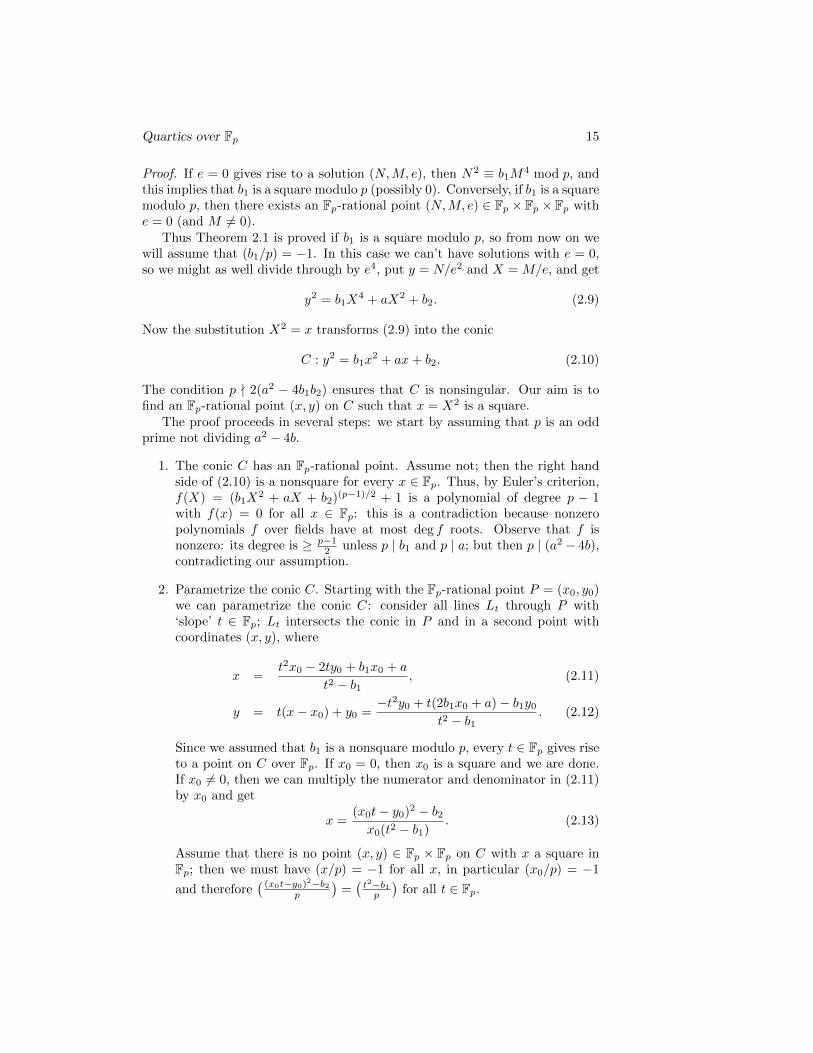
2.2 Quartics over FpConsider the torsor T (b1), with b1 a squarefree integer, over the field Fp. Ouraim is to prove the following
Theorem 2.1. The torsor (2.8) has an Fp-rational point for every prime psuch that p - 2(a2 − 4b).
Remark 1. The polynomial f(X) = b1X4+aX2+b2 has discriminant disc f =
16b(a2−4b)2 = 16b(disc g)2, where g(X) = b1X2+aX+b2. Although p - 2disc g
suffices to guarantee solvability modulo p, for constructing solutions modulo pk
we need to apply Hensel’s Lemma, and this applications forces us to assumethat p - disc f . Thus a torsor T (b1) has a solution in Zp if p - 2b(a2 − 4b); thisis exactly the condition given in [5, Chap. X, Prop. 4.9].
Remark 2. There is a general theorem due to F.K. Schmidt (also proved byChatelet) saying that any smooth curve of genus 1 has a point over any finitefield. Note that the torsors T (b1) are singular at infinity, so one has to be carefulwhen applying this result.
Remark 3. The simple proof of Theorem 2.1 given here is due to Wayne Aitken(San Marcos) and myself.
Quartics over Fp 15
Proof. If e = 0 gives rise to a solution (N,M, e), then N2 ≡ b1M4 mod p, and
this implies that b1 is a square modulo p (possibly 0). Conversely, if b1 is a squaremodulo p, then there exists an Fp-rational point (N,M, e) ∈ Fp × Fp × Fp withe = 0 (and M 6= 0).
Thus Theorem 2.1 is proved if b1 is a square modulo p, so from now on wewill assume that (b1/p) = −1. In this case we can’t have solutions with e = 0,so we might as well divide through by e4, put y = N/e2 and X = M/e, and get
y2 = b1X4 + aX2 + b2. (2.9)
Now the substitution X2 = x transforms (2.9) into the conic
C : y2 = b1x2 + ax+ b2. (2.10)
The condition p - 2(a2 − 4b1b2) ensures that C is nonsingular. Our aim is tofind an Fp-rational point (x, y) on C such that x = X2 is a square.
The proof proceeds in several steps: we start by assuming that p is an oddprime not dividing a2 − 4b.
1. The conic C has an Fp-rational point. Assume not; then the right handside of (2.10) is a nonsquare for every x ∈ Fp. Thus, by Euler’s criterion,f(X) = (b1X
2 + aX + b2)(p−1)/2 + 1 is a polynomial of degree p − 1with f(x) = 0 for all x ∈ Fp: this is a contradiction because nonzeropolynomials f over fields have at most deg f roots. Observe that f isnonzero: its degree is ≥ p−1
2 unless p | b1 and p | a; but then p | (a2 − 4b),contradicting our assumption.
2. Parametrize the conic C. Starting with the Fp-rational point P = (x0, y0)we can parametrize the conic C: consider all lines Lt through P with‘slope’ t ∈ Fp; Lt intersects the conic in P and in a second point withcoordinates (x, y), where
x =t2x0 − 2ty0 + b1x0 + a
t2 − b1, (2.11)
y = t(x− x0) + y0 =−t2y0 + t(2b1x0 + a)− b1y0
t2 − b1. (2.12)
Since we assumed that b1 is a nonsquare modulo p, every t ∈ Fp gives riseto a point on C over Fp. If x0 = 0, then x0 is a square and we are done.If x0 6= 0, then we can multiply the numerator and denominator in (2.11)by x0 and get
x =(x0t− y0)2 − b2x0(t2 − b1)
. (2.13)
Assume that there is no point (x, y) ∈ Fp × Fp on C with x a square inFp; then we must have (x/p) = −1 for all x, in particular (x0/p) = −1
and therefore( (x0t−y0)2−b2
p
)=(t2−b1p
)for all t ∈ Fp.
16 Franz Lemmermeyer 2. Local Solvability
3. By Corollary 2.4 below we have y0 = 0 and b2 = x20b1. This gives 0 =y20 = b1x
20 + ax0 + b2 = b1x
20 + ax0 + b1x
20, hence a = −2b1x0. But then
a2−4b = a2−4b1b2 = 4b21x20−4b1(b1x
20) = 0 contradicting the assumption
that p - (a2 − 4b).
This concludes the proof.
It remains to prove Corollary 2.4. We start with
Lemma 2.2. Let f, g ∈ Fp[X] be quadratic polynomials over Fp. If f(t)n =g(t)n for all t ∈ Fp and some integer n ≤ p−1
2 , then there exists a constantc ∈ Fp such that f = c · g.
Proof. Clearly deg fn = ndeg f ≤ p−1, hence the polynomial fn−gn has degree≤ p− 1 and at least p roots 0, 1, . . . , p− 1. Since Fp is a field, polynomials ofdegree m have at most m roots; hence we conclude that fn = gn.
Now factor f and g into linear factors over some finite extension of Fp; thenevery root α with multiplicity m is a root of multiplicity mn of fn, thus of gn,hence a root of multiplicity m of g. Thus f and g have the same roots (withmultiplicity) over some extension of Fp, hence they are equal up to some constantc (which necessarily is an element of the base field Fp since the coefficients of fand g are).
Proposition 2.3. Assume that f, g ∈ Fp[X] are quadratic polynomials over Fpsuch that ( f(t)p ) = ( g(t)p ) for all t ∈ Fp. Then there exists a constant c ∈ Fp suchthat f = c · g.
Proof. By Euler’s criterion we know that ( f(t)p ) ≡ f(t)n (mod p) with n = p−12 ;
thus the assumptions imply that f(t)n ≡ g(t)n (mod p) for all t ∈ Fp, so theclaim follows from Lemma 2.2.
Remark. It would be interesting to know whether the condition that ( f(t)p ) =
( g(t)p ) for all t ∈ Fp can be weakened.
Corollary 2.4. If( (x0t−y0)2−b2
p
)=(t2−b1p
)for t = 0, 1, . . . , p− 1, then y0 = 0
and b2 = b1x20.
Proof. The converse of the claim is trivially true. On the other hand, applyingProp. 2.3 to the assumption shows that f(X) = (x0X − y0)2 − b2 and g(X) =X2 − b1 differ by a constant factor c; comparing the coefficients of the leadingterm shows that c = x20 whereas comparing linear terms gives y0 = 0. Finally,comparing constant terms shows that b2 = b1x
20.
Reichardt’s Counterexample 17
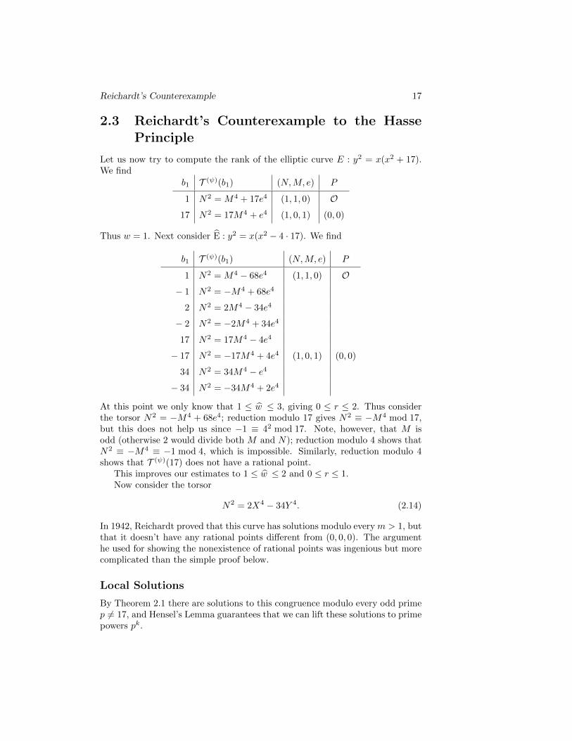
2.3 Reichardt’s Counterexample to the HassePrinciple
Let us now try to compute the rank of the elliptic curve E : y2 = x(x2 + 17).We find
b1 T (ψ)(b1) (N,M, e) P
1 N2 = M4 + 17e4 (1, 1, 0) O
17 N2 = 17M4 + e4 (1, 0, 1) (0, 0)
Thus w = 1. Next consider E : y2 = x(x2 − 4 · 17). We find
b1 T (ψ)(b1) (N,M, e) P
1 N2 = M4 − 68e4 (1, 1, 0) O
− 1 N2 = −M4 + 68e4
2 N2 = 2M4 − 34e4
− 2 N2 = −2M4 + 34e4
17 N2 = 17M4 − 4e4
− 17 N2 = −17M4 + 4e4 (1, 0, 1) (0, 0)
34 N2 = 34M4 − e4
− 34 N2 = −34M4 + 2e4
At this point we only know that 1 ≤ w ≤ 3, giving 0 ≤ r ≤ 2. Thus considerthe torsor N2 = −M4 + 68e4; reduction modulo 17 gives N2 ≡ −M4 mod 17,but this does not help us since −1 ≡ 42 mod 17. Note, however, that M isodd (otherwise 2 would divide both M and N); reduction modulo 4 shows thatN2 ≡ −M4 ≡ −1 mod 4, which is impossible. Similarly, reduction modulo 4shows that T (ψ)(17) does not have a rational point.
This improves our estimates to 1 ≤ w ≤ 2 and 0 ≤ r ≤ 1.Now consider the torsor
N2 = 2X4 − 34Y 4. (2.14)
In 1942, Reichardt proved that this curve has solutions modulo every m > 1, butthat it doesn’t have any rational points different from (0, 0, 0). The argumenthe used for showing the nonexistence of rational points was ingenious but morecomplicated than the simple proof below.
Local Solutions
By Theorem 2.1 there are solutions to this congruence modulo every odd primep 6= 17, and Hensel’s Lemma guarantees that we can lift these solutions to primepowers pk.
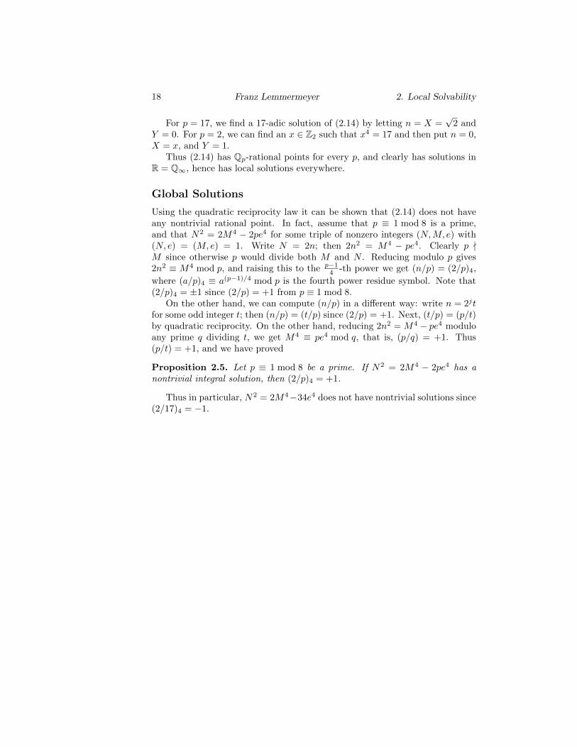
18 Franz Lemmermeyer 2. Local Solvability
For p = 17, we find a 17-adic solution of (2.14) by letting n = X =√
2 andY = 0. For p = 2, we can find an x ∈ Z2 such that x4 = 17 and then put n = 0,X = x, and Y = 1.
Thus (2.14) has Qp-rational points for every p, and clearly has solutions inR = Q∞, hence has local solutions everywhere.
Global Solutions
Using the quadratic reciprocity law it can be shown that (2.14) does not haveany nontrivial rational point. In fact, assume that p ≡ 1 mod 8 is a prime,and that N2 = 2M4 − 2pe4 for some triple of nonzero integers (N,M, e) with(N, e) = (M, e) = 1. Write N = 2n; then 2n2 = M4 − pe4. Clearly p -M since otherwise p would divide both M and N . Reducing modulo p gives2n2 ≡ M4 mod p, and raising this to the p−1
4 -th power we get (n/p) = (2/p)4,
where (a/p)4 ≡ a(p−1)/4 mod p is the fourth power residue symbol. Note that(2/p)4 = ±1 since (2/p) = +1 from p ≡ 1 mod 8.
On the other hand, we can compute (n/p) in a different way: write n = 2jtfor some odd integer t; then (n/p) = (t/p) since (2/p) = +1. Next, (t/p) = (p/t)by quadratic reciprocity. On the other hand, reducing 2n2 = M4 − pe4 moduloany prime q dividing t, we get M4 ≡ pe4 mod q, that is, (p/q) = +1. Thus(p/t) = +1, and we have proved
Proposition 2.5. Let p ≡ 1 mod 8 be a prime. If N2 = 2M4 − 2pe4 has anontrivial integral solution, then (2/p)4 = +1.
Thus in particular, N2 = 2M4−34e4 does not have nontrivial solutions since(2/17)4 = −1.
Lecture 3.Conics
Elliptic curves are nonsingular cubic curves with a rational point and have genus1; conics are quadratic curves and have genus 0. In this lecture we will presenta theory of conics that is closely analogous to that of elliptic curves. First,however, we will talk about parametrization, a technique that only works forcurves of genus 0.
3.1 Parametrization
Parametrization of conics is a technique that allows to find all rational points ona conic if at least one such point is known. Note that there are conics withoutany rational point such as x2 + y2 = 3.
It will be sufficient to present an example: the unit circle C : x2 + y2 = 1.We start with the known point P = (−1, 0) and consider all lines through Pwith slope t: y = t(x + 1). Next we compute the points of intersection of theline and C: we find
0 = x2 + t2(x+ 1)2 − 1 = (x+ 1)(x− 1 + t2(x+ 1)).
The solution to x+1 = 0 corresponds to P ; the solution to x−1+ t2(x+1) = 0,
namely x = 1−t21+t2 , corresponds to the second point of intersection, and we find
y = t(x+ 1) = 2t1+t2 .
Now if t is rational, then these formulas will give a rational point on C.Conversely, if Q = (x, y) is any rational point on C different from P = (−1, 0),then the line through P and Q will have a rational slope t = y
x+1 and willtherefore be given by the formulas above.
3.2 The Group Law
We can study plane algebraic curves both over the affine plane and over theprojective plane. If we want to give elliptic curves a group law, we have to usethe projective plane; similarly, we can give conics a group law as long as westick to the affine plane.
19
20 Franz Lemmermeyer 3. Conics
For the unit circle C : x2 + y2 = 1 over the real numbers we can define agroup law simply by ‘adding angles’: fix a rational point N on C, say N = (1, 0),and define A+B to be the point P such that ∠NOA+ ∠NOB = ∠NOP .
The group law on non-degenerate conics C defined over a field F is quitesimple: fix any rational point N on C; for computing the sum of two rationalpoints A,B ∈ C(F ), draw the line through N parallel to AB, and denote itssecond point of intersection with C by A+B. It is a simple geometric exercise toshow that, in the case of the unit circle in the Euclidean plane, both definitionsagree.
It is straight forward to write down formulas for the addition of points on aconic, but it takes some effort to simplify these formulas to the one given in thenext proposition:
Proposition 3.1. Consider the conic C : X2−dY 2 = c over a field K with oddcharacteristic, and assume that cd 6= 0. Let N = (x, y) be a K-rational pointon C. Then the group law on C with neutral element N is given by
(r, s) + (t, u) =(x(rt+ dsu)− dy(ru+ st)
c,x(ru+ st)− y(rt+ dsu)
c
).
Proof. For adding the points P = (r, s) and Q = (t, u), we have to draw aparallel to the line PQ through N and compute its second point of intersectionwith C.
If P = Q, then the slope m can be computed by taking the derivative of thecurve equation and solving for Y ′; we find Y ′ = x
dy , hence m = rds in P = (r, s).
A simple calculation yields
X =x(r2 + ds2)− 2rsdy
r2 − ds2=x(r2 + ds2)− 2rsdy
c.
Now assume that P 6= Q; if r = t, then (r, s) = P = −Q = (t,−u) andP + Q = N = (x, y), which agrees with the claimed formula. Thus we mayassume that r 6= t; the line through PQ has slope m = s−u
r−t , hence the parallelthrough N is given by the equation Y − y = m(X − x). Intersecting this linewith C leads to
(X − x)[X + x− dm2(X − x)− 2mdy
]= 0;
since X = x gives the point N , the X-coordinate of the second point of inter-section is given by
X =2mdy − (1 + dm2)x
1− dm2.
Plugging in m = s−ur−t , we find
X =2(s− u)(r − t)dy − [(r − t)2 + d(s− u)2]x
(r − t)2 − d(s− u)2.
We now take a closer look at the denominator. We find
(r − t)2 − d(s− u)2 = r2 − ds2 + t2 − du2 − 2rt+ 2dsu = 2(c− rt+ dsu).
The Group Structure 21
Next
(c− rt+ dsu)(ru+ st) = c(r − t)(u− s).
This shows that2y(s− u)(r − t)
(r − t)2 − d(s− u)2= −y(ru+ st)
c;
and that the X-coordinates of both sides agree if x = 0.I haven’t seen yet how to transform the term involving x.
Algebraically, the group law on a conic X2 − aY 2 = c with neutral elementN = (x, y) can be described as follows: identify points (r, s) on the conic withthe algebraic number r + s
√d of norm c; then
(r + s√d ) ∗ (t+ u
√d ) =
(r + s√d )(t+ u
√d )
x+ y√d
corresponds to the point (r, s) + (t, u) on the conic.Proposition 3.1 implies that the group law on conics Y 2−aX2 = 1 is defined
over Z, hence over any ring! In general, the group law of Y 2−aX2 = c is definedover the ring Z[ 1c ].
What about associativity? It is easy to see that associativity of the grouplaw on conics is equivalent to a special case of Pascal’s theorem:
Proposition 3.2. Let ABCPNQ be a hexagon inscribed into a conic. Thenthe points of intersection of the lines AB and PN , BC and NQ, CP and QAare collinear.
The special case we need is when the line containing these points of inter-section is the line at infinity, that is, when the lines in question are parallel inthe affine plane.
For checking that (A+B)+C = A+(B+C), put P = A+B and Q = B+C.Associativity is equivalent to P + C = A + Q, which in turn holds if and onlyif QA ‖ CP . But since AB ‖ PN and BC ‖ NQ by construction and thedefinition of the group law, this follows immediately from Pascal’s theorem.
Exercise. Show that the addition on a parabola P : y = x2 with neutralelement O = (0, 0) is given by (a, a2) + (b, b2) = (c, c2) with c = a+ b; in otherwords: P(R) ' (R,+) is the additive group of the ring over which we work.
Exercise. Show that the addition on a hyperbola H : xy = 1 with neutralelement O = (1, 1) is given by (a, 1/a) + (b, 1/b) = (c, 1/c) with c = ab; in otherwords: H(R) ' R× is the group of units of the ring over which we work.
3.3 The Group Structure
For conics, we have the following nice result (our rings have an identity preservedby ring homomorphisms):
22 Franz Lemmermeyer 3. Conics
Proposition 3.3. If C is a conic defined over Z, and if f : R −→ S is a ringhomomorphism, then f∗(x, y) = (f(x), f(y)) induces a group homomorphismf∗ : C(R) −→ C(S). If f is injective (bijective), then so is f∗.
Proof. A simple exercise. Note that surjectivity of f does not imply surjectivityof f∗.
In particular, the Chinese Remainder Theorem applies to conics in the sensethat
C(Z/NZ) '∏i
C(Z/paiZ)
whenever N =∏i pai , that is, if
Z/NZ '∏i
Z/paiZ.
The structure of C(Fp) for odd primes p and conics C : x2−ny2 = 1 can bedetermined easily: we have
C(Fp) '
{Z/(p− 1)Z if (n/p) = +1
Z/(p+ 1)Z if (n/p) = −1.
In particular, we have #C(Fp) = p− (n/p) for all primes p - 2n.
Primality tests
Proposition 3.4. Let C : x2−dy2 = 1 be a conic, pick N = (1, 0) as the neutralelement, and assume that q ≡ 7 mod 8 is an integer such that (dq ) = −1. Then
q is prime if and only if there exists a point P ∈ C(Z/qZ) such that
i) (q + 1)P = (1, 0);
ii) q+1r P 6= (1, 0) for any prime r dividing (q + 1).
In the special case of Mersenne numbers q = 2p− 1 (note that q ≡ 7 mod 12for p ≥ 3), we have q+1
2 = 2p−1, and if we choose C : x2−3y2 = 1 and P = (2, 1),then the test above is nothing but the Lucas-Lehmer test.
Factorization Methods
The factorization method based on elliptic curves is very well known. Can wereplace the elliptic curve by conics? Yes we can, and what we get is the p− 1-factorization method for integers N if #C(Z/pZ) = p − 1 for all primes p | N(for example if we work with the conic H : xy = 1), the p + 1-factorizationmethod if #C(Z/pZ) = p+ 1 for all p | N , and some hybrid method otherwise.
The only exposition of primality tests and factoring using conics in the math-ematical literature seems to be [9].
The Group Structure 23
3.4 Computing the Rank
Now let us compare the structure of the groups of rational points: for ellipticcurves, we have the famous theorem of Mordell-Weil that E(Q) ' E(Q)tors⊕Zr,where E(Q)tors is the finite group of points of finite order, and r is the Mordell-Weil rank. For conics, on the other hand, we have two possibilities: eitherC(Q) = ∅ (for example if C : x2 + y2 = 3) or C(Q) is infinite, and in fact notfinitely generated (see Tan [8]). The analogy can be saved, however, by lookingat integers instead of rational numbers: Shastri [4] has shown that for the unitcircle C : x2 + y2 = 1 over number fields K we have C(OK) ' Z/4Z ⊕ Zr,where r = s − 1 if K contains a square root of −1, and r = s otherwise; heres is the number of complex primes of K. More generally, we consider rings OSof S-integers for finite sets S of primes; an element of K is an S-integer if itsdenominator is divisible at most by primes in S. Then we find
C(OK) ' C(OK)tors ⊕ Zr E(K) ' E(K)tors ⊕ Zr
where r ≥ 0 is an integer that – in the case of conics x2 − dy2 = 1 – can bedetermined in terms of the number of complex primes in K.
Proposition 3.5. Let C be the conic defined by x2 − dy2 = 1. Let K be anumber field, S a finite set of prime ideals in K, OS the ring of S-integers inK. Then
C(OS) = C(OS)tors ⊕ Zk
for some integer k ≥ 0 and a finite group C(OS)tors.In the special case S = ∅, let r and 2s denote the number of real and complex
embeddings of K. Then OS = OK , and
C(OK) = C(OK)tors ⊕ Zk,
where
k =
r + s− 1 if
√d ∈ K;
r + s if√d 6∈ K and d > 0,
s if√d 6∈ K and d < 0.
Moreover,
C(OK) '
{Z/4Z if d = 1,
Z/2Z if d 6= 1.
The proof given in Shastri [4] works with only minor modifications. Observethat by choosing conics C : x2 − dy2 = c such that the set S of primes dividingc is large, we can make the rank of the group C(ZS) of S-integral points on Carbitrarily large.
Exercise. Let (t, u) be a solution of t2 − u2m = 1; show that (t, u√−m ) is a
solution of x2 + y2 = 1 over Q(√−m ).
24 Franz Lemmermeyer 3. Conics
There is very close analogy between elliptic curves and conics x2 − ny2 = 1:
object conics elliptic curvesgroup structure in affine plane projective planedefined over rings fieldsgroup elements integral points rational pointsgroup structure C(OS)tors ⊕ Zr E(K)tors ⊕ Zrassociativity Pascal’s theorem Bezout’s theorem
Consider x2 − dy2 = 1 over ZS = Z[ 1s ], where S = {p : p | s}. Thendy2 = (x− 1)(x+ 1); write
δ = gcd(x− 1, x+ 1) =
{1 if 2 | x,2 if 2 - x.
Observe that δ = 1 implies d ≡ 3 mod 4.
Assume δ = 2. Then x+ 1 = 2ar2, x− 1 = 2bs2, with ab = d and 2rs = y.Thus 1 = ar2 − bs2.
If d ≡ 3 mod 4 and δ = 1, then x+ 1 = ar2, x− 1 = bs2, where ab = d andrs = y. Thus 2 = ar2 − bs2.
Consider the map α : C(ZS) −→ Q×/Q× 2 defined by
(x, y) 7−→
{2(x+ 1)Q× 2 if x 6= −1,
−dQ× 2 if x = −1.
Note that 2(x+ 1)Q× 2 = aQ× 2 if δ = 2 and 2(x+ 1)Q× 2 = 2aQ× 2 if δ = 1.
Claim. α is a group homomorphism.
Thus given points P = (r, s), Q = (t, u) ∈ C(ZS) we have to show thatα(P )α(Q) = α(P +Q). The left hand side is 2(r+ 1) ·2(t+ 1)Q× 2 = (r+ 1)(t+1)Q× 2; the right hand side equals 2(rt + dsu + 1)Q× 2, and the problem is toshow that (r + 1)(t+ 1) and 2(rt+ dsu+ 1) differ at most by a square factor.
Proposition 3.6. The image of α consists of all square classes δaQ× 2 suchthat ar2 − bs2 = 2/δ has an S-integral solution.
Proof. If δaQ× 2 ∈ imα, then there is a P = (x, y) ∈ C(ZS) such that α(P ) =δaQ× 2, and by our construction above the point P comes from an integral pointon ar2 − bs2 = 2/δ. The converse is also true.
The kernel of α is easy to compute:
Proposition 3.7. We have kerα = 2C(ZS).
The Group Structure 25
This implies that we have an exact sequence
0 −−−−→ 2C(ZS) −−−−→ C(ZS) −−−−→ Q×/Q× 2.
Thus we have C(ZS)/2C(ZS) ' imα; in particular, C(ZS)/2C(ZS) is finitesince #imα | 2s+2. In fact, using the theory of heights (or by generalizingShastri’s proof) we can show that C(ZS) is finitely generated, hence C(ZS) 'C(ZS) ⊕ Zr for some integer r ≥ 0; since C(ZS) is a subgroup of Z/4Z andtherefore cyclic, we have C(ZS)/2C(ZS) ' (Z/2Z)r+1.
Example 1.
Consider C(Z) for C : x2 − 2y2 = 1. The associated curves are
r2 − 2s2 = 1 (r, s) = (1, 0)
2r2 − s2 = 1 (r, s) = (1, 1)
−r2 + 2s2 = 1 (r, s) = (1, 1)
−2r2 + s2 = 1 (r, s) = (1, 0)
Thus C(Z) ' Z/2Z⊕ Z.
Example 2.
Consider C(Z) for C : x2 − 6y2 = 1. The associated curves are
r2 − 6s2 = 1 (r, s) = (1, 0)
2r2 − 3s2 = 1
3r2 − 2s2 = 1 (r, s) = (1, 1)
6r2 − s2 = 1
−r2 + 6s2 = 1
−2r2 + 3s2 = 1 (r, s) = (1, 1)
−3r2 + 2s2 = 1
−6r2 + s2 = 1 (r, s) = (0, 1)
Thus C(Z) ' Z/2Z⊕ Z.
Selmer and Tate-Shafarevich Group
The subset of curves ar2 − bs2 = 2/δ with a rational point corresponds toa subgroup Sel2(C) of Q×/Q× 2 called the 2-Selmer group of C. The Tate-Shafarevich group X2(C) is then defined by the exact sequence
1 −−−−→ imα −−−−→ Sel2(C) −−−−→ X2(C) −−−−→ 1.
In Example 2, the Selmer group is given by Sel2(C) = 〈−2Q× 2, 3Q× 2〉; sinceimα = Sel2(C), we have X2(C) = 0. These calculations are valid in ZS for allfinite sets S.
26 Franz Lemmermeyer 3. Conics
Example 3.
Consider C(Z) for C : x2 − 3y2 = 1. The associated curves are
r2 − 3s2 = 1 (r, s) = (1, 0)
3r2 − s2 = 1
−r2 + 3s2 = 1
−3r2 + s2 = 1 (r, s) = (0, 1)
r2 − 3s2 = 2
3r2 − s2 = 2 (r, s) = (1, 1)
−r2 + 3s2 = 2 (r, s) = (1, 1)
−3r2 + s2 = 2
Thus C(Z) ' Z/2Z⊕ Z.
Example 3.
Consider C(Z) for C : x2 − dy2 = 1; the necessary calculations for producingthe table below are left as an exercise.
d C(Z) Sel2(Z) X2(Z)7 Z/2Z⊕ Z (Z/2Z)2 0
34 Z/2Z⊕ Z (Z/2)3 Z/2Z−1 Z/4Z Z/2Z 0−3 Z/2Z Z/2Z 0−5 Z/2Z Z/2Z 0−6 Z/2Z Z/2Z 0−17 Z/2Z (Z/2Z)2 Z/2Z
Here are some details for d = 34: the associated curves are
r2 − 34s2 = 1 (r, s) = (1, 0)
2r2 − 17s2 = 1 (r, s) = (3, 1)
17r2 − 2s2 = 1 (r, s) = (13 ,
23 )
34r2 − s2 = 1 (r, s) = (13 ,
53 )
−r2 + 34s2 = 1 (r, s) = (53 ,
13 )
−2r2 + 17s2 = 1 (r, s) = (23 ,
13 )
−17r2 + 2s2 = 1 (r, s) = (1, 3)
−34r2 + s2 = 1 (r, s) = (0, 1)
Consider 17r2−2s2 = 1; since it has a rational point, it represents an elementin the Selmer group Sel2(C). We claim that it does not have a nontrivial integral
The Group Structure 27
point. Assume it does; then gcd(r, s) = 1, hence (−2/17)4(s/17) = +1. Now(−1/17)4 = 1; writing s = 2jt we find (s/17) = (t/17) = (17/t) = +1, hencethe existence of an integral point implies (2/17)4 = 1, which is not true.
Thus Sel(C) ' (Z/2)3, C(Z) ' Z/2Z ⊕ Z, and X2(Z) ' Z/2Z; moreover,C(Z3) ' Z/2Z⊕ Z2 and X2(Z3) = 1.
Theorem 3.8. For squarefree integers d, then the conic C : x2 − dy2 = 1 hasTate-Shafarevich group X2(Z) ' Cl +(k)2/Cl +(k)4.
Corollary 3.9. For conics C : x2−dy2 = 1, the Tate-Shafarevich group X2(Z)can have arbitrarily large 2-rank as d varies.
Corollary 3.10. For conics C : x2 − dy2 = 1, the rank of C(ZS) can becomearbitrarily large as d and S vary.
By defining X(Z) for C : x2 − dy2 = 1 using Galois cohomology it shouldbe possible to show that X(Z) ' Cl +(k)2 for k = Q(
√d ).
28 Franz Lemmermeyer 3. Conics
Lecture 4.2-Descent (Proofs)
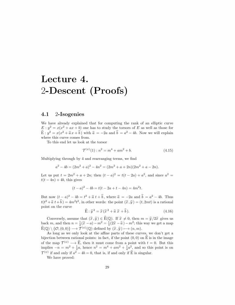
4.1 2-Isogenies
We have already explained that for computing the rank of an elliptic curveE : y2 = x(x2 + ax + b) one has to study the torsors of E as well as those for
E : y2 = x(x2 + a x + b ) with a = −2a and b = a2 − 4b. Now we will explainwhere this curve comes from.
To this end let us look at the torsor
T (ψ)(1) : n2 = m4 + am2 + b. (4.15)
Multiplying through by 4 and rearranging terms, we find
a2 − 4b = (2m2 + a)2 − 4n2 = (2m2 + a+ 2n)(2m2 + a− 2n).
Let us put t = 2m2 + a + 2n; then (t − a)2 = t(t − 2a) + a2, and since a2 =t(t− 4n) + 4b, this gives
(t− a)2 − 4b = t(t− 2a+ t− 4n) = 4m2t.
But now (t − a)2 − 4b = t2 + a t + b , where a = −2a and b = a2 − 4b. Thus
t(t2 + a t+ b ) = 4m2t2, in other words: the point (x , y ) = (t, 2mt) is a rationalpoint on the curve
E : y 2 = x (x 2 + a x + b ). (4.16)
Conversely, assume that (x , y ) ∈ E(Q). If x 6= 0, then m = y /2x gives usback m, and then n = 1
2 (x −a)−m2 = 14 (2x − a )−m2; this way we get a map
E(Q) \ {O, (0, 0)} −→ T (ψ)(Q) defined by (x , y ) 7−→ (n,m).As long as we only look at the affine parts of these curves, we don’t get a
bijection between rational points: in fact, if the point (0, 0) on E is in the image
of the map T (ψ) −→ E, then it must come from a point with t = 0. But thisimplies −n = m2 + 1
2a, hence n2 = m4 + am2 + 14a
2, and so this point is on
T (ψ) if and only if a2 − 4b = 0, that is, if and only if E is singular.We have proved:
29
30 Franz Lemmermeyer 4. 2-Descent (Proofs)
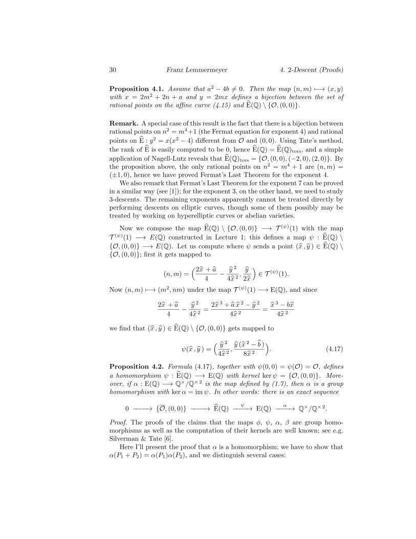
Proposition 4.1. Assume that a2 − 4b 6= 0. Then the map (n,m) 7−→ (x, y)with x = 2m2 + 2n + a and y = 2mx defines a bijection between the set ofrational points on the affine curve (4.15) and E(Q) \ {O, (0, 0)}.
Remark. A special case of this result is the fact that there is a bijection betweenrational points on n2 = m4+1 (the Fermat equation for exponent 4) and rational
points on E : y2 = x(x2 − 4) different from O and (0, 0). Using Tate’s method,
the rank of E is easily computed to be 0, hence E(Q) = E(Q)tors, and a simple
application of Nagell-Lutz reveals that E(Q)tors = {O, (0, 0), (−2, 0), (2, 0)}. Bythe proposition above, the only rational points on n2 = m4 + 1 are (n,m) =(±1, 0), hence we have proved Fermat’s Last Theorem for the exponent 4.
We also remark that Fermat’s Last Theorem for the exponent 7 can be provedin a similar way (see [1]); for the exponent 3, on the other hand, we need to study3-descents. The remaining exponents apparently cannot be treated directly byperforming descents on elliptic curves, though some of them possibly may betreated by working on hyperelliptic curves or abelian varieties.
Now we compose the map E(Q) \ {O, (0, 0)} −→ T (ψ)(1) with the map
T (ψ)(1) −→ E(Q) constructed in Lecture 1; this defines a map ψ : E(Q) \{O, (0, 0)} −→ E(Q). Let us compute where ψ sends a point (x , y ) ∈ E(Q) \{O, (0, 0)}; first it gets mapped to
(n,m) =(2x + a
4− y 2
4x 2,y
2x
)∈ T (ψ)(1).
Now (n,m) 7−→ (m2, nm) under the map T (ψ)(1) −→ E(Q), and since
2x + a
4− y 2
4x 2=
2x 3 + a x 2 − y 2
4x 2=x 3 − bx
4x 2
we find that (x , y ) ∈ E(Q) \ {O, (0, 0)} gets mapped to
ψ(x , y ) =( y 2
4x 2,y (x 2 − b )
8x 2
). (4.17)
Proposition 4.2. Formula (4.17), together with ψ(0, 0) = ψ(O) = O, defines
a homomorphism ψ : E(Q) −→ E(Q) with kernel kerψ = {O, (0, 0)}. More-over, if α : E(Q) −→ Q×/Q× 2 is the map defined by (1.7), then α is a grouphomomorphism with kerα = imψ. In other words: there is an exact sequence
0 −−−−→ {O, (0, 0)} −−−−→ E(Q)ψ−−−−→ E(Q)
α−−−−→ Q×/Q× 2.
Proof. The proofs of the claims that the maps φ, ψ, α, β are group homo-morphisms as well as the computation of their kernels are well known; see e.g.Silverman & Tate [6].
Here I’ll present the proof that α is a homomorphism; we have to show thatα(P1 + P2) = α(P1)α(P2), and we distinguish several cases:
2-Isogenies 31
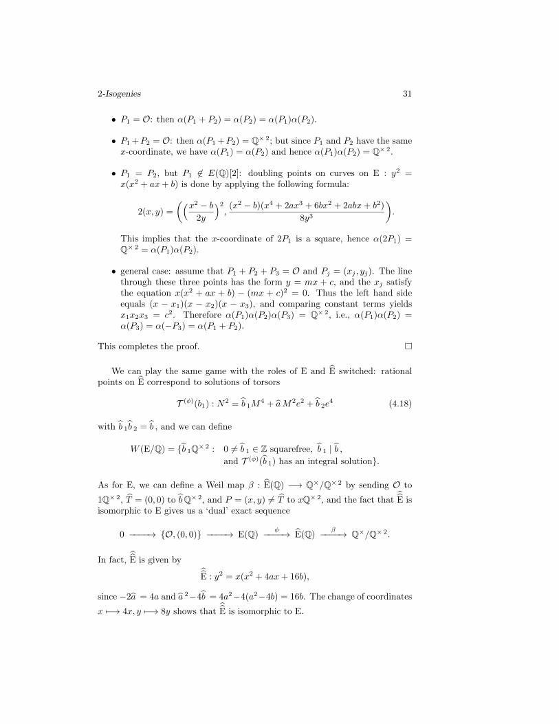
• P1 = O: then α(P1 + P2) = α(P2) = α(P1)α(P2).
• P1 +P2 = O: then α(P1 +P2) = Q× 2; but since P1 and P2 have the samex-coordinate, we have α(P1) = α(P2) and hence α(P1)α(P2) = Q× 2.
• P1 = P2, but P1 6∈ E(Q)[2]: doubling points on curves on E : y2 =x(x2 + ax+ b) is done by applying the following formula:
2(x, y) =
((x2 − b2y
)2,
(x2 − b)(x4 + 2ax3 + 6bx2 + 2abx+ b2)
8y3
).
This implies that the x-coordinate of 2P1 is a square, hence α(2P1) =Q× 2 = α(P1)α(P2).
• general case: assume that P1 + P2 + P3 = O and Pj = (xj , yj). The linethrough these three points has the form y = mx + c, and the xj satisfythe equation x(x2 + ax + b) − (mx + c)2 = 0. Thus the left hand sideequals (x − x1)(x − x2)(x − x3), and comparing constant terms yieldsx1x2x3 = c2. Therefore α(P1)α(P2)α(P3) = Q× 2, i.e., α(P1)α(P2) =α(P3) = α(−P3) = α(P1 + P2).
This completes the proof.
We can play the same game with the roles of E and E switched: rationalpoints on E correspond to solutions of torsors
T (φ)(b1) : N2 = b 1M4 + aM2e2 + b 2e
4 (4.18)
with b 1b 2 = b , and we can define
W (E/Q) = {b 1Q× 2 : 0 6= b 1 ∈ Z squarefree, b 1 | b ,and T (φ)(b 1) has an integral solution}.
As for E, we can define a Weil map β : E(Q) −→ Q×/Q× 2 by sending O to
1Q× 2, T = (0, 0) to bQ× 2, and P = (x, y) 6= T to xQ× 2, and the fact thatE is
isomorphic to E gives us a ‘dual’ exact sequence
0 −−−−→ {O, (0, 0)} −−−−→ E(Q)φ−−−−→ E(Q)
β−−−−→ Q×/Q× 2.
In fact,E is given by
E : y2 = x(x2 + 4ax+ 16b),
since −2a = 4a and a 2−4b = 4a2−4(a2−4b) = 16b. The change of coordinates
x 7−→ 4x, y 7−→ 8y shows thatE is isomorphic to E.
32 Franz Lemmermeyer 4. 2-Descent (Proofs)
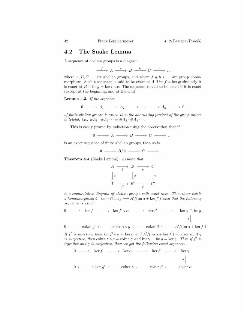
4.2 The Snake Lemma
A sequence of abelian groups is a diagram
f−−−−→ Ag−−−−→ B
h−−−−→ Ci−−−−→ . . .
where A,B,C, . . . are abelian groups, and where f, g, h, i, . . . are group homo-morphism. Such a sequence is said to be exact at A if im f = ker g; similarly itis exact at B if im g = ker i etc. The sequence is said to be exact if it is exact(except at the beginning and at the end).
Lemma 4.3. If the sequence
0 −−−−→ A1 −−−−→ A2 −−−−→ . . . −−−−→ An −−−−→ 0
of finite abelian groups is exact, then the alternating product of the group ordersis trivial, i.e., #A1 ·#A3 · · · = #A2 ·#A4 · · · .
This is easily proved by induction using the observation that if
0 −−−−→ A −−−−→ B −−−−→ C −−−−→ . . .
is an exact sequence of finite abelian groups, then so is
0 −−−−→ B/A −−−−→ C −−−−→ . . .
Theorem 4.4 (Snake Lemma). Assume that
A −−−−→f
B −−−−→g
Cyα yβ yγA′ −−−−→
f ′B′ −−−−→
g′C ′
is a commutative diagram of abelian groups with exact rows. Then there existsa homomorphism δ : ker γ ∩ im g −→ A′/(imα+ ker f ′) such that the followingsequence is exact:
0 −−−−→ ker f −−−−→ ker f ′ ◦ α −−−−→ kerβ −−−−→ ker γ ∩ im g
δ
y0 ←−−−− coker g′ ←−−−− coker γ ◦ g ←−−−− coker β ←−−−− A′/(imα+ ker f ′)
If f ′ is injective, then ker f ′ ◦ α = kerα and A′/(imα + ker f ′) = coker α; if gis surjective, then coker γ ◦ g = coker γ and ker γ ∩ im g = ker γ. Thus if f ′ isinjective and g is surjective, then we get the following exact sequence:
0 −−−−→ ker f −−−−→ kerα −−−−→ kerβ −−−−→ ker γ
δ
y0 ←−−−− coker g′ ←−−−− coker γ ←−−−− coker β ←−−−− coker α
Tate’s formula 33
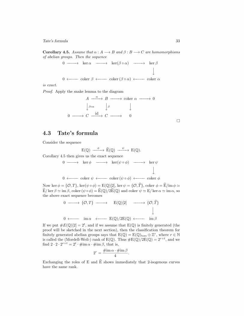
Corollary 4.5. Assume that α : A −→ B and β : B −→ C are homomorphismsof abelian groups. Then the sequence
0 −−−−→ kerα −−−−→ ker(β ◦ α) −−−−→ kerβy0 ←−−−− coker β ←−−−− coker (β ◦ α) ←−−−− coker α
is exact.
Proof. Apply the snake lemma to the diagram
Aα−−−−→ B −−−−→ coker α −−−−→ 0yβ◦α yβ y
0 −−−−→ Cid−−−−→ C −−−−→ 0
4.3 Tate’s formula
Consider the sequence
E(Q)φ−−−−→ E(Q)
ψ−−−−→ E(Q).
Corollary 4.5 then gives us the exact sequence
0 −−−−→ kerφ −−−−→ ker(ψ ◦ φ) −−−−→ kerψy0 ←−−−− coker ψ ←−−−− coker (ψ ◦ φ) ←−−−− coker φ
Now kerφ = {O, T}, ker(ψ ◦φ) = E(Q)[2], kerψ = {O, T}, coker φ = E/imφ 'E/ kerβ ' imβ, coker (ψ ◦φ) = E(Q)/2E(Q) and coker ψ ' E/ kerα ' imα, sothe above exact sequence becomes
0 −−−−→ {O, T} −−−−→ E(Q)[2] −−−−→ {O, T}y0 ←−−−− imα ←−−−− E(Q)/2E(Q) ←−−−− imβ
If we put #E(Q)[2] = 2t, and if we assume that E(Q) is finitely generated (theproof will be sketched in the next section), then the classification theorem forfinitely generated abelian groups says that E(Q) = E(Q)tors ⊕ Zr, where r ∈ Nis called the (Mordell-Weil-) rank of E(Q). Thus #E(Q)/2E(Q) = 2r+t, and wefind 2 · 2 · 2r+t = 2t ·#imα ·#imβ, that is,
2r =#imα ·#imβ
4.
Exchanging the roles of E and E shows immediately that 2-isogenous curveshave the same rank.
34 Franz Lemmermeyer 4. 2-Descent (Proofs)
4.4 Heights
Let us now quickly sketch the theory of heights which is needed for the sec-ond part of the proof of the theorem of Mordell-Weil. Recall that the heightH(x) of rational numbers x = m
n with gcd(m,n) = 1 was defined as H(x) =max{|m|, |n|}.
Our first task is to study how heights change when x is replaced by f(x) forsome polynomial f ∈ Z[X].
Lemma 4.6. If f(X) = anXn + . . . + a1X + a0 ∈ Z[X], then H(f(x)) ≤
(n+ 1)mH(x)n for all x ∈ Q, where m = max{|a0|, |a1|, . . . , |an|}.
We shall give the proof to give you an idea of the techniques used here:
Proof. Write x = pq with gcd(p, q) = 1; then H(x) = max{|p|, |q|}, and in
particular we have |p| ≤ H(x) and |q| ≤ H(x). Now
|qnf(x)| = |anpn + an−1pn−1q + . . .+ a1q
n−1p+ a0qn|
≤ |an||p|n + |an−1||p|n−1|q|+ . . .+ |a1||p||q|n−1 + |a0||q|n
≤ (n+ 1)mH(x)n,
because |ak| ≤ m and |p|r|q|n−r ≤ H(x)rH(x)n−r = H(x)n.
Finding a lower bound of the same order of magnitude is much more difficult.Yet it can be done:
Lemma 4.7. Let f, g ∈ Z[X] be coprime, and put n = max{deg f, deg g}. Thenthere exist constants C1, C2 > 0 such that for all x ∈ Q we have
C1H(x)n ≤ H(f(x)
g(x)
)≤ C2H(x)n.
The proof of this lemma is elementary but rather involved.The height of a rational point P ∈ E(Q) on an elliptic curve E is defined by
H(P ) =
{1 if P = O,H(x) if P = (x, y).
It is often convenient to use the logarithmic height h(P ) = logH(P ).A first simple observation is the following:
Lemma 4.8. Let E be an elliptic curve defined over Q. Then for all κ > 0, theset {P ∈ E(Q) : H(P ) < κ} of rational points with bounded height is finite.
The height on elliptic curves satisfies certain relations that will be needed inour proof of the Mordell-Weil theorem. We’ll start with
Lemma 4.9. Let E an elliptic curve defined over Q. Then there exists someC > 0 such that H(2P ) ≥ CH(P )4 for all P ∈ E(Q).
Selmer and Tate-Shafarevich Groups 35
The second estimate we need is
Lemma 4.10. Let E be an elliptic curve defined over Q, and let P0 ∈ E(Q).Then there is a C0 > 0 such that H(P + P0) ≤ C0H(P )2 for all P ∈ E(Q).
Both of these lemmas are simple applications of Lemma 4.7. Now we canprove
Theorem 4.11 (Mordell’s Theorem). Let E be an elliptic curve defined overQ. If E(Q)/2E(Q) is finite, then E(Q) is finitely generated.
Proof. The following proof is taken from the notes [7] of Bart de Smit. Notethat we have proved that E(Q)/2E(Q) is finite for elliptic curves E : y2 =x(x2 + ax+ b).
Let S be a set of rational points P on E such that the P represent all cosetsof E(Q)/2E(Q). Since E(Q)/2E(Q) is finite, we can choose S to be finite aswell.
By Lemma 4.10, for each Pj ∈ S there is a constant cj > 0 such thatH(Q − Pj) ≤ cjH(Q)2. Thus for C = max{cj : Pj ∈ S} (here we use the factthat E(Q)/2E(Q) is finite) we have H(Q − P ) ≤ C · H(Q)2 for all Q ∈ E(Q)and all P ∈ S. Moreover, we have H(2Q) ≥ C−11 H(Q)4 for all Q ∈ E(Q).
Now let T denote the union of S and the (finitely many) rational pointsR ∈ E(Q) of height H(R) < B := 4
√C1C. We claim that E(Q) is generated by
the points in T .We shall prove this by induction on the height. Clearly every Q ∈ E(Q) with
H(Q) < B is generated by a point in T since Q ∈ T .Now assume that all rational points of height < h are generated by points
in T , and assume that H(Q) < 2h. There is a P ∈ S such that Q − P = 2R,and we find
H(R)4 ≤ C1 ·H(Q− P ) ≤ C1C ·H(Q)2.
If H(R) > H(Q)/2, thenH(Q)4/16 < H(R)4 ≤ C1C ·H(Q)2, that is, H(Q) < Band therefore Q ∈ T ; if H(R) ≤ H(Q)/2 = h, then R is generated by points inT by induction assumption, hence so is Q = P + 2R.
4.5 Selmer and Tate-Shafarevich Groups
For computing the rank of an elliptic curve E : y2 = x(x2 + ax+ b) we have todecide whether certain torsors have rational points or not, that is, we have tocompute #imα and #imβ. This is a difficult problem. On the other hand, it isrelatively easy to decide whether these torsors have local solutions everywhere,that is, whether they have solutions modulo all prime powers and in the reals.The classes b1Q× 2 corresponding to such everywhere locally solvable torsorsT (ψ)(b1) (these are the torsors that have solutions modulo every prime power
as well as real solutions) form a group Sel(ψ)(E/Q) containing W (E/Q) := imαas a subgroup. The following exact sequence then defines the ψ-part of theTate-Shafarevich group of E:
0 −−−−→ W (E/Q) −−−−→ Sel(ψ)(E/Q) −−−−→ X(E/Q)[ψ] −−−−→ 0
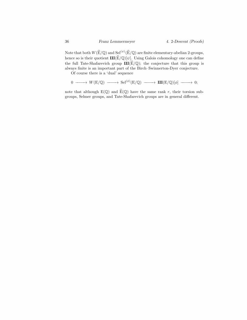
36 Franz Lemmermeyer 4. 2-Descent (Proofs)
Note that bothW (E/Q) and Sel(ψ)(E/Q) are finite elementary-abelian 2-groups,
hence so is their quotient X(E/Q)[ψ]. Using Galois cohomology one can define
the full Tate-Shafarevich group X(E/Q); the conjecture that this group isalways finite is an important part of the Birch–Swinnerton-Dyer conjecture.
Of course there is a ‘dual’ sequence
0 −−−−→ W (E/Q) −−−−→ Sel(φ)(E/Q) −−−−→ X(E/Q)[φ] −−−−→ 0;
note that although E(Q) and E(Q) have the same rank r, their torsion sub-groups, Selmer groups, and Tate-Shafarevich groups are in general different.
Lecture 5.Nontrivial Elements in qq[2]
In this lecture we will present various techniques for constructing nontrivialelements in the Tate-Shafarevich group.
5.1 Pepin’s Claims
The following is taken from [1].It is well known that curves of genus 0 defined over Q satisfy the Hasse
principle: they have a rational point if and only if they have a Qp-rational pointfor every completion Qp of Q. It is similarly well known that the Hasse principlefails to hold for curves of genus 1, the first counter example 2z2 = x4 − 17y4
being due to Lind [Li] and Reichardt [Re].In a series of articles [P1, P2, P3, P4], Theophile Pepin announced 93 the-
orems asserting that certain equations of the type aX4 + bY 4 = Z2 were notsolvable in integers (nontrivially, that is). In order to get nontrivial results,Pepin looks at equations whose underlying conics ax2 + by2 = z2 do have ratio-nal solutions (see [P1]):
Les cas ou l’equation indeterminee aX4 + bY 4 = Z2 n’admet pasde solution rationnelle sont fort nombreux, meme quand l’equationax2 + by2 = z2 est resoluble en nombres entiers. Neanmoins on neconnait encore qu’un petit nombre de theoremes sur ce sujet.
He then starts listing his results without proof, and among his examples thereare some that claim the nonexistence of rational points on some curves of genus 1that are everywhere locally solvable. To the best of my knowledge no proofs forPepin’s claims have been supplied yet. The proofs that we give below are basedon connections with the 2-class groups of complex quadratic number fields.
5.2 Applications of Genus Theory
Let us start with the following assertion taken from [P2]:
37
38 Franz Lemmermeyer 5. Nontrivial Elements in X
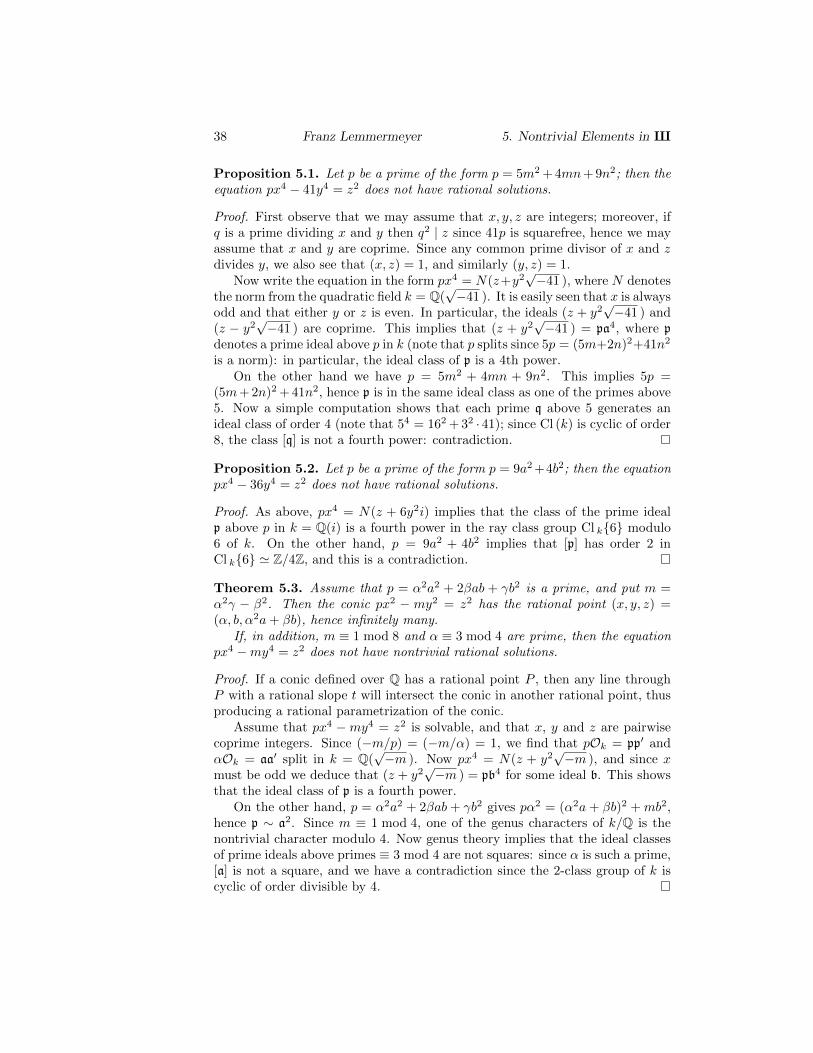
Proposition 5.1. Let p be a prime of the form p = 5m2 + 4mn+ 9n2; then theequation px4 − 41y4 = z2 does not have rational solutions.
Proof. First observe that we may assume that x, y, z are integers; moreover, ifq is a prime dividing x and y then q2 | z since 41p is squarefree, hence we mayassume that x and y are coprime. Since any common prime divisor of x and zdivides y, we also see that (x, z) = 1, and similarly (y, z) = 1.
Now write the equation in the form px4 = N(z+y2√−41 ), where N denotes
the norm from the quadratic field k = Q(√−41 ). It is easily seen that x is always
odd and that either y or z is even. In particular, the ideals (z + y2√−41 ) and
(z − y2√−41 ) are coprime. This implies that (z + y2
√−41 ) = pa4, where p
denotes a prime ideal above p in k (note that p splits since 5p = (5m+2n)2+41n2
is a norm): in particular, the ideal class of p is a 4th power.On the other hand we have p = 5m2 + 4mn + 9n2. This implies 5p =
(5m+ 2n)2 + 41n2, hence p is in the same ideal class as one of the primes above5. Now a simple computation shows that each prime q above 5 generates anideal class of order 4 (note that 54 = 162 + 32 · 41); since Cl (k) is cyclic of order8, the class [q] is not a fourth power: contradiction.
Proposition 5.2. Let p be a prime of the form p = 9a2 +4b2; then the equationpx4 − 36y4 = z2 does not have rational solutions.
Proof. As above, px4 = N(z + 6y2i) implies that the class of the prime idealp above p in k = Q(i) is a fourth power in the ray class group Cl k{6} modulo6 of k. On the other hand, p = 9a2 + 4b2 implies that [p] has order 2 inCl k{6} ' Z/4Z, and this is a contradiction.
Theorem 5.3. Assume that p = α2a2 + 2βab + γb2 is a prime, and put m =α2γ − β2. Then the conic px2 − my2 = z2 has the rational point (x, y, z) =(α, b, α2a+ βb), hence infinitely many.
If, in addition, m ≡ 1 mod 8 and α ≡ 3 mod 4 are prime, then the equationpx4 −my4 = z2 does not have nontrivial rational solutions.
Proof. If a conic defined over Q has a rational point P , then any line throughP with a rational slope t will intersect the conic in another rational point, thusproducing a rational parametrization of the conic.
Assume that px4 −my4 = z2 is solvable, and that x, y and z are pairwisecoprime integers. Since (−m/p) = (−m/α) = 1, we find that pOk = pp′ andαOk = aa′ split in k = Q(
√−m ). Now px4 = N(z + y2
√−m ), and since x
must be odd we deduce that (z + y2√−m ) = pb4 for some ideal b. This shows
that the ideal class of p is a fourth power.On the other hand, p = α2a2 + 2βab+ γb2 gives pα2 = (α2a+ βb)2 +mb2,
hence p ∼ a2. Since m ≡ 1 mod 4, one of the genus characters of k/Q is thenontrivial character modulo 4. Now genus theory implies that the ideal classesof prime ideals above primes ≡ 3 mod 4 are not squares: since α is such a prime,[a] is not a square, and we have a contradiction since the 2-class group of k iscyclic of order divisible by 4.
Pepin’s Claims 39
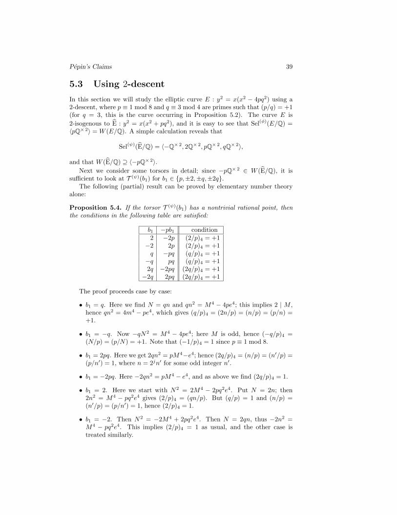
5.3 Using 2-descent
In this section we will study the elliptic curve E : y2 = x(x2 − 4pq2) using a2-descent, where p ≡ 1 mod 8 and q ≡ 3 mod 4 are primes such that (p/q) = +1(for q = 3, this is the curve occurring in Proposition 5.2). The curve E is
2-isogenous to E : y2 = x(x2 + pq2), and it is easy to see that Sel(φ)(E/Q) =〈pQ× 2〉 = W (E/Q). A simple calculation reveals that
Sel(ψ)(E/Q) = 〈−Q× 2, 2Q× 2, pQ× 2, qQ× 2〉,
and that W (E/Q) ⊇ 〈−pQ× 2〉.Next we consider some torsors in detail; since −pQ× 2 ∈ W (E/Q), it is
sufficient to look at T (ψ)(b1) for b1 ∈ {p,±2,±q,±2q}.The following (partial) result can be proved by elementary number theory
alone:
Proposition 5.4. If the torsor T (ψ)(b1) has a nontrivial rational point, thenthe conditions in the following table are satisfied:
b1 −pb1 condition2 −2p (2/p)4 = +1−2 2p (2/p)4 = +1q −pq (q/p)4 = +1−q pq (q/p)4 = +12q −2pq (2q/p)4 = +1−2q 2pq (2q/p)4 = +1
The proof proceeds case by case:
• b1 = q. Here we find N = qn and qn2 = M4 − 4pe4; this implies 2 | M ,hence qn2 = 4m4 − pe4, which gives (q/p)4 = (2n/p) = (n/p) = (p/n) =+1.
• b1 = −q. Now −qN2 = M4 − 4pe4; here M is odd, hence (−q/p)4 =(N/p) = (p/N) = +1. Note that (−1/p)4 = 1 since p ≡ 1 mod 8.
• b1 = 2pq. Here we get 2qn2 = pM4−e4; hence (2q/p)4 = (n/p) = (n′/p) =(p/n′) = 1, where n = 2jn′ for some odd integer n′.
• b1 = −2pq. Here −2qn2 = pM4 − e4, and as above we find (2q/p)4 = 1.
• b1 = 2. Here we start with N2 = 2M4 − 2pq2e4. Put N = 2n; then2n2 = M4 − pq2e4 gives (2/p)4 = (qn/p). But (q/p) = 1 and (n/p) =(n′/p) = (p/n′) = 1, hence (2/p)4 = 1.
• b1 = −2. Then N2 = −2M4 + 2pq2e4. Then N = 2qn, thus −2n2 =M4 − pq2e4. This implies (2/p)4 = 1 as usual, and the other case istreated similarly.
40 Franz Lemmermeyer 5. Nontrivial Elements in X
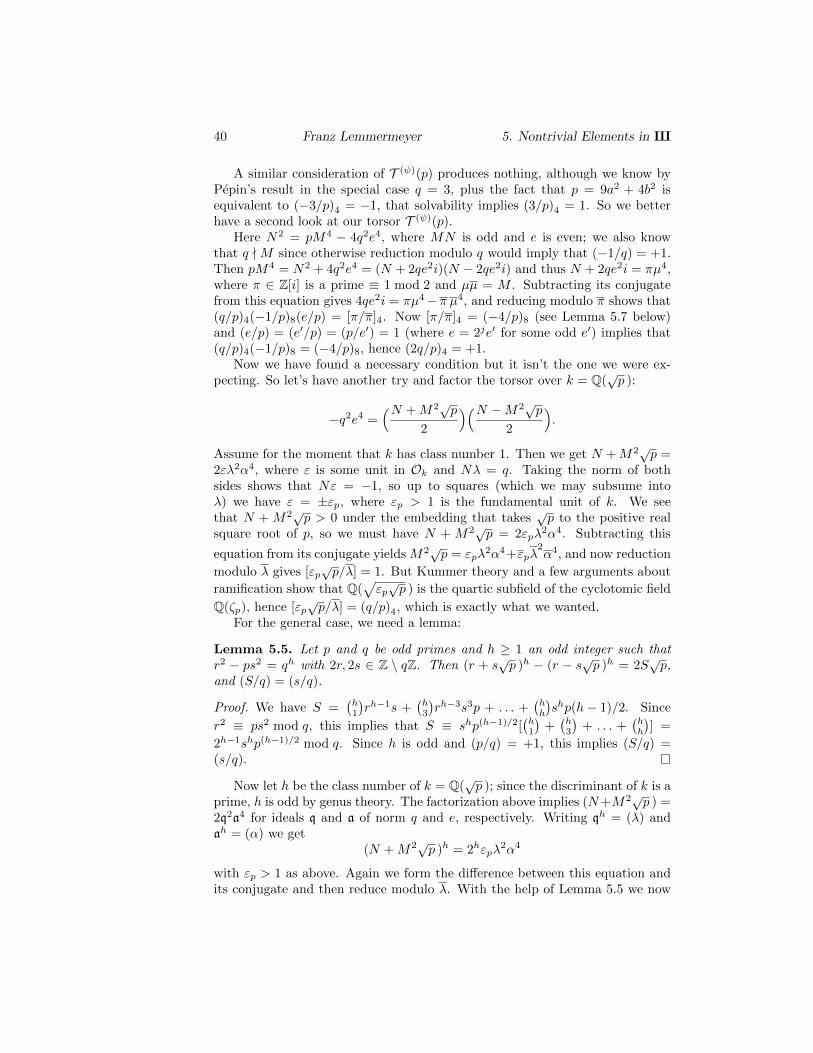
A similar consideration of T (ψ)(p) produces nothing, although we know byPepin’s result in the special case q = 3, plus the fact that p = 9a2 + 4b2 isequivalent to (−3/p)4 = −1, that solvability implies (3/p)4 = 1. So we betterhave a second look at our torsor T (ψ)(p).
Here N2 = pM4 − 4q2e4, where MN is odd and e is even; we also knowthat q -M since otherwise reduction modulo q would imply that (−1/q) = +1.Then pM4 = N2 + 4q2e4 = (N + 2qe2i)(N − 2qe2i) and thus N + 2qe2i = πµ4,where π ∈ Z[i] is a prime ≡ 1 mod 2 and µµ = M . Subtracting its conjugatefrom this equation gives 4qe2i = πµ4−π µ4, and reducing modulo π shows that(q/p)4(−1/p)8(e/p) = [π/π]4. Now [π/π]4 = (−4/p)8 (see Lemma 5.7 below)and (e/p) = (e′/p) = (p/e′) = 1 (where e = 2je′ for some odd e′) implies that(q/p)4(−1/p)8 = (−4/p)8, hence (2q/p)4 = +1.
Now we have found a necessary condition but it isn’t the one we were ex-pecting. So let’s have another try and factor the torsor over k = Q(
√p ):
−q2e4 =(N +M2√p
2
)(N −M2√p2
).
Assume for the moment that k has class number 1. Then we get N +M2√p =2ελ2α4, where ε is some unit in Ok and Nλ = q. Taking the norm of bothsides shows that Nε = −1, so up to squares (which we may subsume intoλ) we have ε = ±εp, where εp > 1 is the fundamental unit of k. We seethat N + M2√p > 0 under the embedding that takes
√p to the positive real
square root of p, so we must have N + M2√p = 2εpλ2α4. Subtracting this
equation from its conjugate yields M2√p = εpλ2α4+εpλ
2α4, and now reduction
modulo λ gives [εp√p/λ] = 1. But Kummer theory and a few arguments about
ramification show that Q(√εp√p ) is the quartic subfield of the cyclotomic field
Q(ζp), hence [εp√p/λ] = (q/p)4, which is exactly what we wanted.
For the general case, we need a lemma:
Lemma 5.5. Let p and q be odd primes and h ≥ 1 an odd integer such thatr2 − ps2 = qh with 2r, 2s ∈ Z \ qZ. Then (r + s
√p )h − (r − s√p )h = 2S
√p,
and (S/q) = (s/q).
Proof. We have S =(h1
)rh−1s +
(h3
)rh−3s3p + . . . +
(hh
)shp(h− 1)/2. Since
r2 ≡ ps2 mod q, this implies that S ≡ shp(h−1)/2[(h1
)+(h3
)+ . . . +
(hh
)] =
2h−1shp(h−1)/2 mod q. Since h is odd and (p/q) = +1, this implies (S/q) =(s/q).
Now let h be the class number of k = Q(√p ); since the discriminant of k is a
prime, h is odd by genus theory. The factorization above implies (N+M2√p ) =2q2a4 for ideals q and a of norm q and e, respectively. Writing qh = (λ) andah = (α) we get
(N +M2√p )h = 2hεpλ2α4
with εp > 1 as above. Again we form the difference between this equation andits conjugate and then reduce modulo λ. With the help of Lemma 5.5 we now
Pepin’s Claims 41
see that [√p/λ] = [εp/λ], and this proves as above that (q/p)4 = 1 is necessary
for T (ψ)(p) to be solvable.We summarize our discussion in the following
Theorem 5.6. Consider the elliptic curve E : y2 = x(x2 − 4pq2), where p ≡1 mod 8 and q ≡ 3 mod 4 are primes such that (p/q) = +1. If the torsorT (ψ)(p) : N2 = pM4−4q2e4 has a rational solution, then (2/p)4 = (q/p)4 = +1.
Moreover, we always have X(E/Q)[2] = 0, and X(E/Q)[2] has order divisibleby 4 unless possibly when (2/p)4 = (q/p)4 = +1.
Our results aren’t as complete as we might want them: if (2/p)4 = 1 and(q/p)4 = −1, for example, then we know that the torsors T (ψ)(b1) are not solv-able for b1 ∈ {−1, q,−q}, and we also know that one of T (ψ)(2) and T (ψ)(−2) is
not solvable (assuming the finiteness of X(E/Q) we can even predict that ex-actly one of them is solvable), but we can not tell which. It would be interestingto find criteria that allow us to do this.
We still have to provide a proof for
Lemma 5.7. Let π = a + bi be a prime in Z[i] with norm p ≡ 1 mod 8, andassume that 4 | b and a ≡ 1 mod 4. Then [π/π]4 = (−4/p)8.
Proof. Since π = a + bi ≡ 2bi mod π, we find [π/π]4 = [2iπ]4[b/π]4. Now[2i/π]4 = (−4/p)8 since −4 = (2i)2, hence it is sufficient to prove that [b/π]4 =1.
Assume first that b ≡ 4 mod 8; then b = 4b′ for some odd b′, and using[−1/π]4 = +1 we find [b/π]4 = (2/p)[b′/π]4 = [b′/π]4 = [π/b′]4 = [a/b′]4. Butquartic residue symbols whose entries are rational integers are trivial and ourclaim follows. If 8 | b, then [2/π]4 = (2/p)4 = +1, hence writing b = 2jb′ forsome odd b′ gives [b/π]4 = [b′/π]4 = [π/b′]4 = [a/b′]4 = +1.
References
[Li] C.-E. Lind, Untersuchungen uber die rationalen Punkte der ebenen kubi-schen Kurven vom Geschlecht Eins, Diss. Univ. Uppsala 1940
[P1] Th. Pepin, Theoremes d’analyse indeterminee, C. R. Acad. Sci. Paris 78(1874), 144–148
[P2] Th. Pepin, Theoremes d’analyse indeterminee, C. R. Acad. Sci. Paris 88(1879), 1255–1257
[P3] Th. Pepin, Nouveaux theoremes sur l’equation indeterminee ax4 + by4 =z2, C. R. Acad. Sci. Paris 91 (1880), 100–101
[P4] Th. Pepin, Nouveaux theoremes sur l’equation indeterminee ax4 + by4 =z2, C. R. Acad. Sci. Paris 94 (1882), 122–124
[Re] H. Reichardt, Einige im Kleinen uberall losbare, im Großen unlosbare dio-phantische Gleichungen, J. Reine Angew. Math. 184 (1942), 12–18
42 Franz Lemmermeyer 5. Nontrivial Elements in X
Lecture 6.3-Descent
The computation of the Mordell-Weil groups of certain elliptic curves usingsimple 2-descent worked for curves with a rational 2-torsion point. The ‘simple’3-descent works for elliptic curves with a rational 3-torsion point, and, in fact,more generally for curves with a ‘rational’ 3-torsion group.
The first 3-descent was used by Euler in his (almost complete) proof ofFermat’s Last Theorem for the exponent 3. More recently, Selmer [Se], Cassels[C1, C2], Quer [Qu], Satge [S1, S2], Top [To], Yen-Mei Julia Chen [Ch] and M.DeLong [D1] worked out the theory of 3-descents.
6.1 3-Descent on Curves with Rational 3-Torsion
Consider the elliptic curve
E : y2 = x3 +D2. (6.19)
The points T = (0, D) and −T = (0,−D) are torsion points of order 3, and{O,±T} is a subgroup of the torsion group E(Q)tors; in fact, it is equal toE(Q)[3]. (Observe that y2 = x3 + c6 has at least six torsion points generated by(−c2, 0) + (0, c3).)
By Lemma 1.6, every rational point (x, y) 6= O on E(Q) has the form x =m/e2, y = n/e3 for integers n,m, e such that (m, e) = (n, e) = 1. Plugging thisinto E gives
m3 = n2 −D2e6 = (n−De3)(n+De3).
Put d = gcd(n − De3, n + De3); then d divides 2n and 2De3, hence d |gcd(2n, 2De3) = 2 gcd(n,De3) = 2 gcd(n,D). Write 2D = dD1 and m = dm1;
since n−De3d and n+De3
d are coprime and since their product equals m3/d2 =dm3
1, we findn−De3 = dd1a
3, n+De3 = dd2b3 (6.20)
with d1d2 = d and ab = m1. Subtracting the equations (6.20) from each otherand canceling d gives
D1e3 = d2b
3 − d1a3.
43
44 Franz Lemmermeyer 6. 3-Descent
Observe that d1d2D1 = dD1 = 2D.We have proved:
Proposition 6.1. Every rational point (x, y) 6= O on (6.19) gives rise to arational point (u, v, w) on
Ta,b : au3 + bv3 + cw3 = 0, (6.21)
where a, b, c ∈ Z satisfy abc = 2D.Conversely, any rational point (u, v, w) on (6.21) yields a rational point on
(6.19): we find
e = w; m = −abuv; n = a2bu3 +Dw3,
hence
(x, y) =(−abuv
w2,a2bu3 +Dw3
w3
).
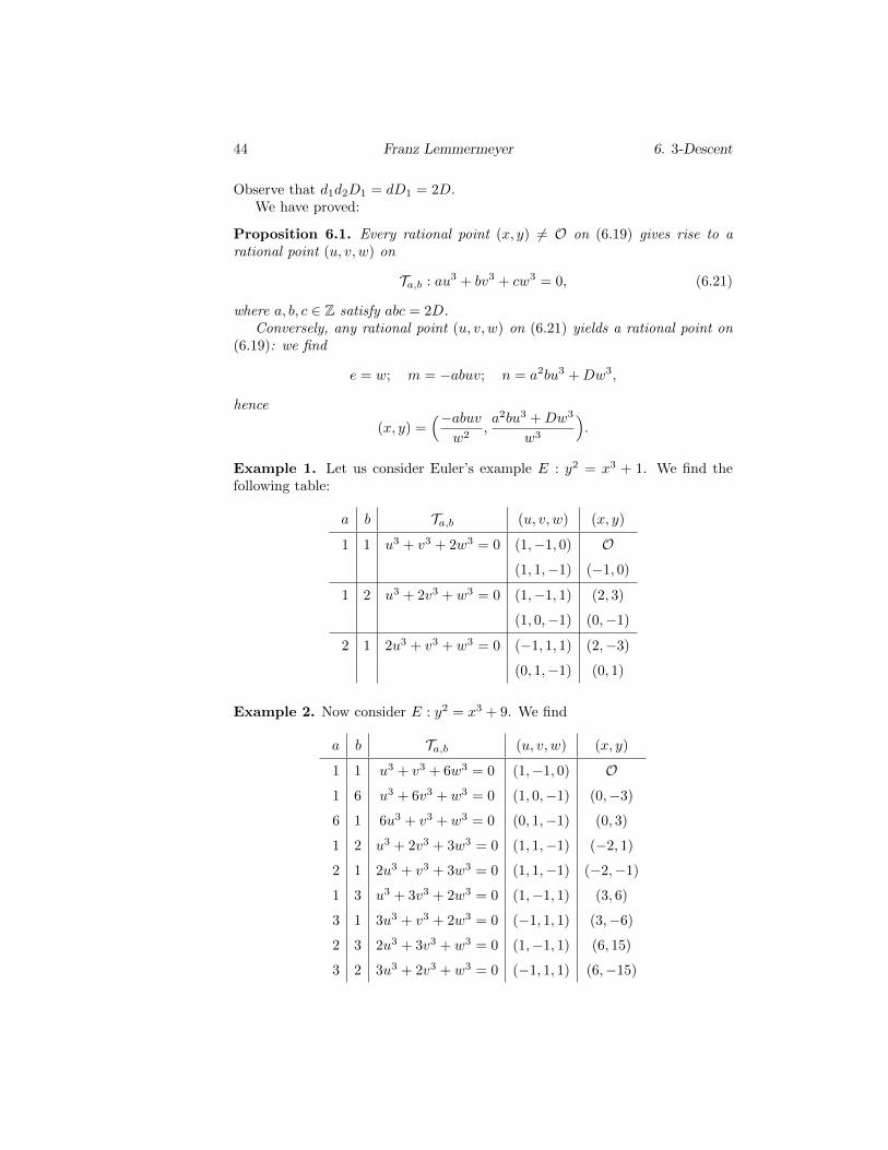
Example 1. Let us consider Euler’s example E : y2 = x3 + 1. We find thefollowing table:
a b Ta,b (u, v, w) (x, y)
1 1 u3 + v3 + 2w3 = 0 (1,−1, 0) O
(1, 1,−1) (−1, 0)
1 2 u3 + 2v3 + w3 = 0 (1,−1, 1) (2, 3)
(1, 0,−1) (0,−1)
2 1 2u3 + v3 + w3 = 0 (−1, 1, 1) (2,−3)
(0, 1,−1) (0, 1)
Example 2. Now consider E : y2 = x3 + 9. We find
a b Ta,b (u, v, w) (x, y)
1 1 u3 + v3 + 6w3 = 0 (1,−1, 0) O
1 6 u3 + 6v3 + w3 = 0 (1, 0,−1) (0,−3)
6 1 6u3 + v3 + w3 = 0 (0, 1,−1) (0, 3)
1 2 u3 + 2v3 + 3w3 = 0 (1, 1,−1) (−2, 1)
2 1 2u3 + v3 + 3w3 = 0 (1, 1,−1) (−2,−1)
1 3 u3 + 3v3 + 2w3 = 0 (1,−1, 1) (3, 6)
3 1 3u3 + v3 + 2w3 = 0 (−1, 1, 1) (3,−6)
2 3 2u3 + 3v3 + w3 = 0 (1,−1, 1) (6, 15)
3 2 3u3 + 2v3 + w3 = 0 (−1, 1, 1) (6,−15)
The 3-Isogenous Curve 45
So far, everything is analogous to to the situation of 2-descents on curveswith a rational point of order 2. There, the torsor analogous to T1,1 turned out
to be isomorphic to an elliptic curve E, and there was a 2-isogeny E −→ E.Something similar holds here:
Proposition 6.2. Over any field of characteristic not dividing 6, the torsorT1,1 : u3 + v3 + 2Dw3 = 0 is isomorphic to the elliptic curve
E : y2 = x3 − 27D2, (6.22)
and the composition E −→ T1,1 −→ E is a 3-isogeny, that is, a homomorphismbetween elliptic curves with a kernel of order 3.
6.2 The 3-Isogenous Curve
We would like to go on as in the case of 2-descents, but at this point we runinto trouble: the elliptic curve E : y2 = x3 − 27D2 does not have the formy2 = x3 + d2, and it fact does not have a rational point of order 3: it seemsthat our approach breaks down. There is, however, a way to get around thisproblem: just work over Q(
√−3 ), where −27D2 = (3
√−3D)2 is a square.
Using the arithmetic in Z[ρ], where ρ2 + ρ+ 1 = 0, we get as above
m3 = n2 + 27D2e6 = (n+ 3√−3De3)(n− 3
√−3De3).
Let δ = gcd(n+ 3√−3De3, n− 3
√−3De3) denote the greatest common divisor
of the two factors on the right.
Lemma 6.3. We have δ ∈ Z or δ ∈ 3√−3Z.
Proof. This follows directly from δ | (n+3√−3De3) and δ | (n+3
√−3De3).
Clearly δ divides 2n and 2D√−3
3e3, hence δ | 2 gcd(n,
√−3
3D). Now there
are two cases:
1. δ ∈ Z. Then unique factorization in Z[ρ] shows
n− 3√−3De3 = δδ1α
3, n+ 3√−3De3 = δδ2β
3,
where δ1δ2 = δ, and where we have absorbed units into the δi. Since bothelements on the left hand side are conjugate, and since δ ∈ Z, we musthave β = ±α and δ2 = ±δ1.
2. δ ∈ 3√−3Z. Then δ = 3
√−3δ′ for some δ′ ∈ Z, as well as n = 9n′, hence
dividing both sides through by 3√−3 and repeating the argument above
shows that
n− 3√−3De3 = δδ1(α
√−3 )3, n+ 3
√−3De3 = δδ2(−α
√−3 )3,
where δ1δ2 = δ′ and δ2 is the conjugate of δ1.
46 Franz Lemmermeyer 6. 3-Descent
We can subsume both cases into one by putting
τ =
{1 if δ ∈ Z;√−3 if δ ∈ 3
√−3Z.
Observing that
n+ 3√−3De3 = δ21δ2(τα)3, n− 3
√−3De3 = δ1δ
22(τα)3,
and putting ν = δ2/δ1 we find ν = ν−1, hence
n+ 3√−3De3 = νγ3, n− 3
√−3De3 = ν−1γ3,
where γ = δ1τα. Thus
νγ3 − ν−1γ3 = 2D(√−3e)3.
Dividing through by√−3
3and putting µ = γ/
√−3, µ = −γ/
√−3 (note that
µ still is the conjugate of µ), we get
νµ3 + ν−1µ3 = 2De3.
Now write ν = a+b√−3
a−b√−3 and put
u =1
2
( µ
a− b√−3
+µ
a+ b√−3
),
v =1
2√−3
( µ
a− b√−3− µ
a+ b√−3
),
w = e
Then u, v, w ∈ Q satisfy the equation
au3 − 9bu2v − 9auv2 + 9bv3 =D
a2 + 3b2w3. (6.23)
In fact, put r = µa−b√−3 and s = µ
a+b√−3 ; then
u3 =1
8(r3 + 3r2s+ 3rs2 + s3)
u2v =1
24
√−3(r3 + r2s− rs2 − s3)
uv2 =1
24(r3 − r2s− rs2 + s3)
v3 =1
72
√−3(r3 − 3r2s+ 3rs2 − s3),
hence the sum of the terms involving r3 in (6.23) becomes ( 4a8 −
4b8
√−3 )r3 =
12 (a − b
√−3 )r3 = νµ3/2(a2 + 3b2). Similarly, we find that the terms involving
The Rank Formula 47
r2s and rs2 add up to 0, whereas those involving s3 add up to a+b√−3
2 s3 =ν−1µ/2(a2 + 3b2). Thus
au3 − 9bu2v − 9auv2 + 9bv3 =1
2(a2 + 3b2)(νµ3 + ν−1µ3)
=1
2(a2 + 3b2)(2De3) =
D
a2 + 3b2w3.
Proposition 6.4. Every rational point (X,Y ) on E : Y 2 = X3 − 27D2 givesrise to a rational point (x, y, z) on one of the torsors
Ta,b : au3 − 9bu2v − 9auv2 + 9bv3 =D
a2 + 3b2w3,
where a, b ∈ Z are determined as follows: write X = m/e3, Y = n/e3, and letd = gcd(n+ 3
√−3e3, n+ 3
√−3e3). Then d ∈ Z and 4d = a2 + 3b2. Conversely,
every rational point (u, v, w) on Ta,b gives rise to a rational point on E.
Example 1. Consider E : y2 = x3 + 1; then E : y2 = x3 − 27. Here δ = 1,hence
a b Ta,b (u, v, w) (x, y)
1 0 u3 − 9uv2 = w3 (0, 1, 0) O
(1, 0, 1) (3, 0)
− 12
12 u3 + 9uv2 − 9uv2 − 9v3 = 2w3
− 12 − 1
2 u3 − 9uv2 − 9uv2 + 9v3 = 2w3
The two torsors corresponding to (a, b) = (− 12 ,±
12 ) are not solvable modulo 9
since 2 is not a cube modulo 9.
Example 2. Consider E : y2 = x3 + 9; then E : y2 = x3 − 243.
a b Ta,b (u, v, w) (x, y)
1 0 u3 − 9uv2 = 3w3 (0, 1, 0) O
(3, 1, 0)
(3, 2,−3) (7, 10)
6.3 The Rank Formula
Consider the elliptic curveEk : y2 = x3 + k (6.24)
48 Franz Lemmermeyer 6. 3-Descent
where k ∈ Z is assumed to be free of sixth powers. Define
k′ =
{−27k if 27 - k,− k
27 if 27 | k.
Note that (k′)′ = k for all integers k not divisible by 36. These curves alwayshave a rational group of 3-torsion points, that is, a group of three points killedby 3 and invariant under the action of Gal (Q/Q).
Theorem 6.5. Put
δ =
{1 if 27 - k,3 if 27 | k.
The map φ : Ek −→ Ek′ defined by
P 7−→
{O, if 3P = O, i.e.P = O, (0,±
√k );(
x3+4k(δx)2 , y(x
3−8k)(δx)2
), if P = (x, y), 3P 6= O,
is an isogeny of degree 3 defined over Q. If ψ denotes the corresponding isogenyEk′ −→ Ek, then ψ ◦ φ = [3] is multiplication by 3 on Ek, and φ ◦ ψ = [3] ismultiplication by 3 on Ek′ .
Proof.
Now put F = Q(√k ). We define a map α : Ek(Q) −→ F×/F× 3 by
α(P ) =
1 · F× 3 if P = O,1
2√k· F× 3 if P = (0,−
√k ),
(y +√k ) · F× 3 if P = (x, y), P 6= (0,−
√k ).
Note that the second line only applies if P ∈ Ek(Q), that is, if k is a square. We
can similarly define a map β : Ek′(Q) −→ F ′×/F ′× 3
defined over the quadraticnumber field F ′ = Q(
√k′ ) = Q(
√−3k ).
Theorem 6.6. We have the following exact sequences:
Ek′(Q)ψ−−−−→ Ek(Q)
α−−−−→ F×/F× 3,
Ek(Q)φ−−−−→ Ek′(Q)
β−−−−→ F ′×/F ′× 3.
Proof.
Consider the sequence
Ek(Q)φ−−−−→ Ek′(Q)
ψ−−−−→ Ek(Q);
as before we get the exact sequence
0 −−−−→ kerφ −−−−→ Ek(Q)[3] −−−−→ kerψy0 ←−−−− imα ←−−−− Ek(Q)/3Ek(Q) ←−−−− imβ
The Image of α and β 49
We find
#Ek(Q)[3] =
{3 if k = −432 or
√k ∈ Q;
1 otherwise;
# kerφ =
{3 if
√k ∈ Q,
1 otherwise;
# kerψ =
{3 if
√−3k ∈ Q,
1 otherwise;
in particular
3u := # kerφ ·# kerψ =
{3 if
√k ∈ Q or
√−3k ∈ Q,
1 otherwise.
Now let 3t = #Ek(Q)[3] with t ∈ {0, 1}; then #Ek(Q)/3Ek(Q) = 3r+t, hence
3r =#imα ·#imβ
# kerφ ·# kerψ.
Note that kerψ = 0 if k is a square; thus 3r+1 = #imα ·#imβ in this case.In particular, E : y2 = x3 + 1 has rank 0.
6.4 The Image of α and β
Now we will have to characterize the image of α and β.
Proposition 6.7. We have
imα ⊆
{Q×/Q× 3 if
√k ∈ Q;
kerN if√k 6∈ Q,
where N : F×/F× 3 −→ Q×/Q× 3 is the homomorphism defined by N(α·F× 3) =NF/Qα ·Q× 3.
Proof.
References
[C1] J.W. Cassels, The rational solutions of the diophantine equation y2 =x3 −D, Acta Math. 82 (1950), 243–273
[C2] J.W. Cassels, Arithmetic on curves of genus 1. I. On a conjecture ofSelmer, J. Reine Angew. Math. 202 (1959), 52–99
50 Franz Lemmermeyer 6. 3-Descent
[Ch] Y.-M. J. Chen, Descent via 3-isogenies on elliptic curves, Ph.D. Diss.Brown Univ. 1993
[D1] M. DeLong, Relating elliptic curves to 3-ranks of quadratic number fields,Ph.D. thesis Univ. Michigan, 1988
[D2] M. DeLong, A formula for the Selmer group of a rational 3-isogeny,
[Ge] J. Gebel,
Diss. Univ. Saarbrucken
[Qu] J. Quer, Sobre el 3-rang dels cossos quadraticos i la corba elliptica y2 =x3 +M , Ph.D. thesis Barcelona 1987
[S1] Ph. Satge, Une generalisation du calcul de Selmer, Semin. Theor. Nom-bres Paris, 1981–82 (1983), 245–265
[S2] Ph. Satge, Groupes de Selmer et corps cubiques, J. Number Theory 23(1986), 294–317
[Se] E.S. Selmer, The diophantine equation ax3 + by3 + cz3 = 0, Acta Math.85 (1951), 203–362
[To] J. Top, Descent by 3-isogeny and 3-rank of quadratic fields, Adv. NumberTheory (1993), 303–317
Bibliography
[1] F. Lemmermeyer, A note on Pepin’s counter examples to the Hasse prin-ciple for curves of genus 1, Abh. Math. Sem. Hamburg 69 (1999), 335–34530, 37
[2] F. Lemmermeyer, On Tate-Shafarevich groups of some elliptic curves, Proc.Conf. Graz 1998, (2000), 277–291
[3] F. Lemmermeyer, Some families of non-congruent numbers, Acta Arith.,to appear
[4] P. Shastri, Integral points on the unit circle, J. Number Theory 91 (2001),67–70 23
[5] J. Silverman, The arithmetic of elliptic curves, Springer-Verlag 14
[6] J. Silverman, J. Tate, Rational points on elliptic curves, Springer-Verlag30
[7] B. de Smit, Handouts, Seminar Leiden 2001, athttp://www.math.leidenuniv.nl/∼desmit/ell/ 35
[8] Lin Tan, The group of rational points on the unit circle, Math. Mag. 69(1996), no. 3, 163–171 23
[9] M.Z. Zhang, Factoring integers with conics (Chinese. English summary),Sichuan Duxue Xuebao 33 (1996), 356–359 22
51