Computers & Geosciences, Vol. 3, pp. 341-346. Pergamon Press, 1977. Printed in Great Britain

REGULARIZATIO� OF A SEMIVARIOGRAM

ISOBEL CLARK

Department of Mineral Resources Engineering, Imperial College of Science and Technology,

Prince Consort Road, London SW7 2BP, England

(Received 1 October 1976)

Abstract - The production of estimates using the technique of kriging, and the evaluation of the

accuracy of these estimates depends completely on the production of a model for the

semivariogram of the deposit. The process of choosing such a model can be complicated in

practice by the bulk and geometry of the samples taken. Some aspects of this problem are

discussed and some formulae and a FORTRAN IV subroutine are presented to ease the task of

modeling.

Key Words: FORTRAN, Kriging, Regionalized variables, Semivariogram.

I�TRODUCTIO�

It has been said that the semivariogram is the basic tool of the Theory of Regionalized Variables.

The computation of an experimental semivariogram may be tedious, but rarely difficult. It is in

the interpretation and fitting of a model to a practical semivariogram that the real difficulties

arise. For instance, to carry out a kriging exercise of any type, we require for the deposit a

theoretical model of the semivariogram. This model produces for us the relationship between

two points a certain distance apart. Note, however, that we said points. Seldom in practice can

we measure a value, say the grade of a mineral, at a point. At the feasibility stage of mine

development we are concerned mostly with borehole cores; during development and production

we may have many different types of samples, but all of them have one thing in common. They

have a certain bulk, a certain geometrical shape and volume. In some instances, they may be

assayed using different techniques. All of these factors combine to form the "support" of the

samples. A semivariogram which has been calculated on one type of support will not be the

same as that calculated on another. The process, of averaging the grade over the bulk of a

sample, will influence the shape and behavior in such a manner that we must use an indirect

method to derive the theoretical model for the point semivariogram necessary to further analysis

and estimation.

REGULARIZATIO�

Suppose that we had a line of n point samples at regular intervals along a line (say a drive or a

raise). For example in Figure 1 points on the experimental semivariogram may be calculated

with ease:

These points may be plotted on a graph of γ* vs h, and a model for the point semivariogram

chosen and fitted directly to the data points.

Now suppose that, instead of a line of point samples, we are concerned with a borehole which

has been assayed in sections of length 1. We no longer know the assay value at some point x, but

rather the average value over a length (x− /2, x+ /2). How will this affect the semivariogram?

Let us consider the problem from an intuitive point of view.

Consider two segments, or "cores", of length a distance h apart as in Figure 2. Suppose that

we knew the grade at every point along both of those segments. Then we could calculate γ*(h)

for all the pairs of points, that distance h apart, by computing the difference in grade for each

pair, squaring the result, and averaging through all the pairs. However, suppose that we do not

know the grade at every point, but only the average grade of each segment. The semivariogram

calculated then must be denoted by

γ *(h), and this will be computed by taking the difference in the average grades, squaring and

averaging those. However, to obtain the average grade of the segment, all the variation of grades

within the segment has been eliminated. Thus, the average grade of the segment will be a more

regular variable than the average grade of individual points. If the variable is more regular, this

implies that the differences between any two of the values will be less. That is γ *(h) will of

necessity be less in value than the corresponding γ*(h), whatever the form of γ*(h). Now

consider those models for γ*(h) which possess a sill, and therefore a range of influence. Two

points which are farther apart than the range of influence, a, may be said to be independent. But,

two segments whose centers are a distance a apart will not be independent of one another,

because one-half of one segment will be within the range of influence of one-half of the other

segment. It is not until h = a + , that is the ends of the segments are a apart, that no point in

one segment influences the other. Thus, for a point model γ*(h) with a certain range of

influence, it is manifest that γ *(h) will have a range of influence units larger. This

phenomenon of the change in character of the semivariogram as the support of the sample

changes is known as regularization, and γ *(h) is termed the regularized semivariogram.

REGULARIZATIO� OF THE USUAL MODELS

The mathematics of the process of regularization are in Matheron (1971), and need not be

discussed here. However, it may be of advantage to outline the effect of regularization on the

more usual models of the semivariogram. The linear model of γ*(h) is the most widely used of

those without a sill, and is characterized by:

For samples of length , we determine that:

That is, for distances greater than - which is all we have in practice - the regularized

semivariogram is a straight line with the same slope as the point model, but with an intercept on

the γ axis of - p /3 (see Fig. 3), if the semivariogram is not complicated by a nugget effect.

Thus, the model for the point semivariogram may be obtained by estimating the slope for the

regularized semivariogram.

There are two usual models for semivariograms with a sill. The exponential model:

When regularized by , this becomes:

With a somewhat more complex form for the parabolic part with h< . The sill of this

regularized semivariogram obviously will be lower than the sill of the corresponding point

model. This can be shown to be:

We have experimentally values of the regularized semivariogram, that is γ *(h) for various

values of h< . We need to be able to estimate the parameters of the point semivariogram, a and

C, from γ * in some manner. Having done this, we may substitute these values into the equation

(1) to give 'theoretical' points on γ , for comparison with γ *.

The first step is to plot a graph of γ * against h (see Fig. 4). From this we can estimate C

immediately as the asymptote of the curve. In practice, of course, γ * will be more irregular. A

first approximation for a, now may be determined. Draw a straight line through the first few

points on γ * and extend it until it meets the sill level C . The value of h at which the two meet

should be approximately a . We have seen that a = a + , so an estimate for a follows

immediately.

Having estimated C and a (if only approximately) equation (2) may be used to determine an

approximation for C. These values, a and C, then may be used in equation (1) to produce values

of γ (h). Plotting these points on the same graph as γ *(h) will give a visual comparison

between the model and the data. The parameters can be adjusted if necessary to improve the fit,

and the process repeated. For example, if all the values of γ were slightly higher than the

corresponding γ *, either the estimate of the range of influence is too small or the estimate of the

sill is too high, or both. Visual inspection should reveal which. The process is repeated until we

produce a γ (h) which seems "close enough" to γ *(h) for our satisfaction. The final values of a

and C then can be used to characterize the point semivariogram for the deposit.

The third model - and perhaps the one in widest use in mineral valuation - is the spherical or

Matheron model. This semivariogram, expressed as:

is the popular one which exhibits linear behavior near the origin, gradually curves off, until at h

= a it reaches its sill and stays there permanently. Many mineral deposits seem to conform to

this sort of behavior, but the discontinuity in the formula renders the mathematical handling

more complex than the other models. This discontinuity also divides the resulting formula for γ

(h) into a series of alternatives given various boundary conditions on h and a. These formulae

will not be given in the text, but are presented in Appendix I in the form of a FORTRAN IV

subroutine which will be described more fully in a later section. However, we can say that the

relationship between the sill of γ (h) and that of γ(h) is given by:

If the linear behavior for the first few points of γ(h) is extended to meet the sill, the distance at

which this occurs is 2a/3 (see Fig. 5). So, we may approximate a and C as follows:

• guess C , the sill of the regularized semivariogram;

• produce the line through the first few points up to C , to give h = 2a /3, and hence a

;

• a = a - as before;

• calculate C from the appropriate part of equation (3);

• use attached subroutine to produce values of γ (h) using a and C;

• plot or graph; compare with γ *(h);

• adjust a and C if necessary; repeat, etc.

When a satisfactory fit has been obtained, we have the point spherical model for the deposit and

may proceed with estimation and kriging.

SUBROUTI�E REGSPH

The subroutine included in Appendix I is a FORTRAN IV routine to evaluate points of a

regularized spherical semivariogram given the following information;

NH - number of points to be evaluated.

A - range of influence of the point semivariogram.

C - sill of the point semivariogram

EL - length of samples producing regularization.

H - array containing values of h for which γ (h) is to be calculated

The subroutine is evoked by:

CALL REGSPH (GL, H, NH, A, C, EL)

and returns in array GL the values of the semivariogram γ (h) for the corresponding values of h

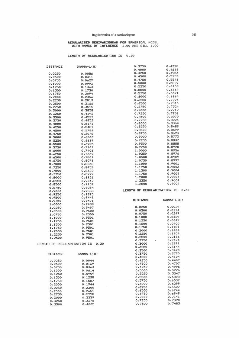
in H. Note that the distances in H need not be in ascending order. To assist the user in

implementing the subroutine and checking for possible mispunches, a program segment and

printout are included in Appendix II.

Acknowledgments The subroutine REGSPH was developed on the CDC 6400 installation at

Imperial College, London and the program and subroutine implemented on the DEC system-10

at Syracuse University, Syracuse, New York, while the author was Visiting Associate Professor

in the Department of Geology.

REFERE�CE

Matheron, G., 1971, The theory of regionalized variables and its applications: Cahiers du Centre

de Morphologie Mathematique de Fontainebleau, no. 5, 211 p.

APPE�DIX I