Regional Variation in Rental Costs for Larger Households

Arthur Grimes, Robert Sourell & Andrew Aitken

Motu Working Paper 05 - 02

Motu Economic and Public Policy Research

May 2005

© 2005 Motu Economic and Public Policy Research Trust. All rights reserved. No portion of this paper may be reproduced without permission of the authors. Motu Working Papers are research materials circulated by their authors for purposes of information and discussion. They have not necessarily undergone formal peer review or editorial treatment. ISSN 1176-2667.

Author contact details Arthur Grimes Motu Economic and Public Policy Research arthur.grimes@motu.org.nz Andrew Aitken Motu Economic and Public Policy Research andrew.aitken@motu.org.nz Robert Sourell Motu Economic and Public Policy Research robert@sourell.de Acknowledgements The authors thank the Ministry of Housing for access to tenancy bond data and Quotable Value New Zealand for provision of property price data. The Centre for Housing Research Aotearoa New Zealand (CHRANZ) provided funding for an earlier project that sparked our interest in the current topic; we thank Terrence Aschoff and CHRANZ for their ongoing interest in this and related work. We also thank our Motu colleagues for extremely helpful comments on a presentation of an early draft of this material.

Motu Economic and Public Policy Research PO Box 24390 Wellington New Zealand Email: info@motu.org.nz Telephone: +64-4-939-4250 Website: www.motu.org.nz

Abstract Housing costs comprise a major part of most household budgets. Larger

households require greater space than do smaller households but do not

necessarily have larger incomes. The cost of extra housing space (e.g. the cost of

an extra bedroom) may vary across different locations, both absolutely (dollars

per week) and proportionately (percentage of overall costs). If this is the case,

differential regional costs of additional space may provide an incentive for

different sized households to locate in particular areas where housing costs most

appropriately fit their needs. Our analysis uses tenancy bond rental data to analyse

the cost of renting an extra bedroom in different locations throughout New

Zealand. It discusses the theory of what determines rents. We then examine the

nature of regional rental costs, testing whether the documented patterns fit with

theoretical predictions. Finally, we reflect on what the results may imply for social

outcomes and housing policy in New Zealand. To give a flavour of the issues,

consider the following. In 2003, the average weekly rental cost of a two bedroom

dwelling in Auckland was $37 more than for a one bedroom dwelling. The cost of

a third bedroom was an extra $50 and the cost of a fourth bedroom was an

additional $90. Thus weekly rental cost for a four bedroom dwelling exceeded that

of a one bedroom dwelling by $177. In Manawatu-Wanganui, the cost of a two

bedroom dwelling was $38 more than for a one bedroom dwelling - almost

identical to the margin in Auckland. But the cost of additional bedrooms was

much lower than in Auckland: $29 for a third bedroom and $33 for a fourth

bedroom. This raw data might suggest that it would be beneficial for larger

households to locate in Manawatu-Wanganui and for smaller households to locate

in Auckland. However, the interaction with other factors has to be taken into

account before such a conclusion can be reached. At the minimum, the data

suggests there is a material issue to be addressed relating to disparities in regional

housing costs for different sized households.

JEL classification: R21; R31; R51 Keywords: House Rents; Deprivation; Regional Disparities

Contents

1 Introduction .....................................................................................................1

2 Theory..............................................................................................................5 2.1 General Aspects ......................................................................................5 2.2 Application..............................................................................................7

3 Data................................................................................................................10 3.1 Datasets .................................................................................................10 3.2 QVNZ data............................................................................................11 3.3 Tenancy bond data ................................................................................13

4 Relationship Between Rents & Prices ...........................................................14

5 Rental Costs of Extra Bedrooms ...................................................................24

6 Implications ...................................................................................................29

References ..............................................................................................................33

Appendix A : Rent/Price Relationships .................................................................34

Appendix B: Capital Gains Relationships..............................................................39

Table of figures Figure 1: Rent/Price Ratio (Houses) Related to Deprivation Index Score...............3

Figure 2: Identifying spurious sale prices ..............................................................12

Figure 3: Distribution of House Prices for New Zealand, 2001 ............................13

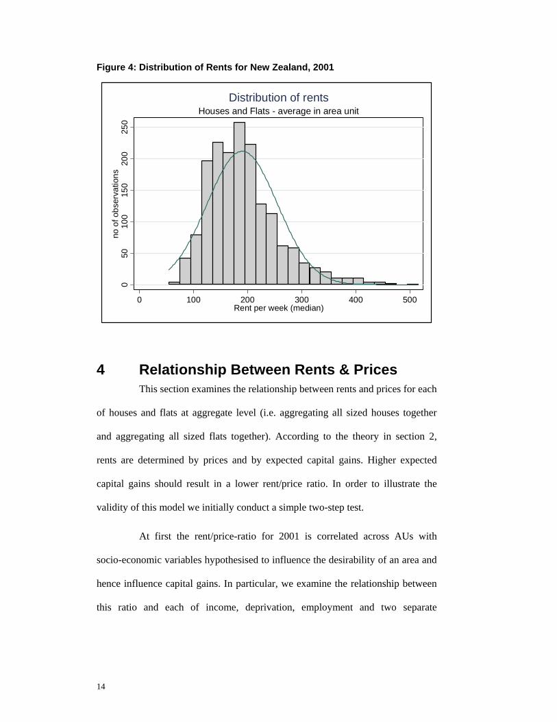
Figure 4: Distribution of Rents for New Zealand, 2001 ........................................14

Table of tables Table 1: Significant relationships between socio-economic factors & the

rent/price-ratio.........................................................................................15

Table 2: Impact of socio-economic factors on capital gains (2001/1996) .............16

Table 3: Results of estimating (7): Houses (Non-Linear)*....................................18

Table 4: Results of estimating (7): Apartments (Non-Linear)* .............................19

Table 5: Results of estimating (8): Houses (Linear)* ............................................22

Table 6: Results of estimating (8): Apartments (Linear)* .....................................23

Table 7: Results of estimating (9)* ........................................................................25

Table 8: Effect of Variables on Rents ($ per week) - OLS (2001 data)*...............27

Table 9: Effect of Variables on Rents ($ per week) - IV (1996 data)*..................27

1

1 Introduction Housing costs represent a large proportion of total income for many

households. In 2001, 33% of households spent at least a quarter of their income on

housing; 15% of households spent more than two-fifths of their income on

housing. Housing costs can therefore have a significant impact on living standards

for many people, and may be particularly germane for lower income households

that rent. One of the nine variables that comprise the deprivation index for New

Zealand is "not living in own home" (Crampton et al, 2000). While covering a

number of categories, the majority of people covered by this variable will be

renters. An understanding of the determinants of rents across different localities is

therefore vital for understanding the determinants of overall living standards,

especially for more deprived households.

Large families have a greater need for housing services than do smaller

families. A family with one child may receive quite satisfactory housing quality

through their rental of a one or two bedroom house or apartment, but a five child

household may need at least a four bedroom house to achieve the same housing

quality. In understanding living standard outcomes of large households, we

therefore need to understand the determinants of housing costs - in this case,

rentals - for dwellings of different sizes.1

In this study, we examine the determinants of rents for houses and

apartments of different sizes across locations in New Zealand. Initially, we

analyse the relationship of rents to house prices aggregating together houses of all

sizes and apartments of all sizes (but maintaining a segregation between houses

1 Henceforth "dwellings" refers to the combined set of houses and apartments; "size" refers to number of bedrooms. The terms "apartment" and "flat" are used interchangeably.

2

and apartments). We then extend our analysis to determining the costs of extra

bedrooms in houses across locations.

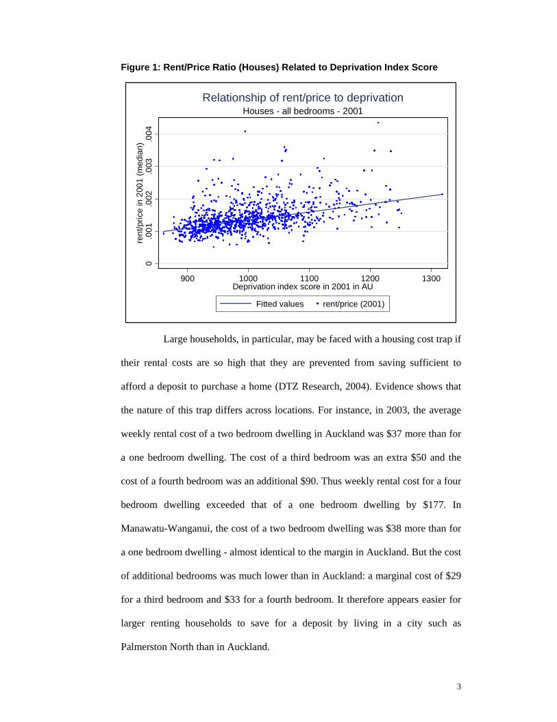
House prices can be taken as a summary statistic for the way purchasers

value the location, amenity and housing characteristics in each locality (Can,

1992; Dubin, 1992; Grimes et al, 2003; Grimes and Aitken, 2004; Meen, 2001). It

might therefore be reasonable to expect that rentals will be proportionate to house

prices across locations. But this is not the case. Using 2001 data for New Zealand

(discussed in greater detail in section 3), Figure 1 demonstrates that, on average,

rents are high relative to house prices in locations that have high levels of

deprivation (an increase in the deprivation scale indicates a more deprived area).

Given that more deprived households have a greater likelihood of renting than do

less deprived households (Crampton et al, 2000) these relationships imply that

such households may be caught in a housing cost trap. One contribution of this

paper is to analyse the reasons behind the existence of this trap.

3

Figure 1: Rent/Price Ratio (Houses) Related to Deprivation Index Score

0.0

01.0

02.0

03.0

04re

nt/p

rice

in 2

001

(med

ian)

900 1000 1100 1200 1300Deprivation index score in 2001 in AU

Fitted values rent/price (2001)

Houses - all bedrooms - 2001Relationship of rent/price to deprivation

Large households, in particular, may be faced with a housing cost trap if

their rental costs are so high that they are prevented from saving sufficient to

afford a deposit to purchase a home (DTZ Research, 2004). Evidence shows that

the nature of this trap differs across locations. For instance, in 2003, the average

weekly rental cost of a two bedroom dwelling in Auckland was $37 more than for

a one bedroom dwelling. The cost of a third bedroom was an extra $50 and the

cost of a fourth bedroom was an additional $90. Thus weekly rental cost for a four

bedroom dwelling exceeded that of a one bedroom dwelling by $177. In

Manawatu-Wanganui, the cost of a two bedroom dwelling was $38 more than for

a one bedroom dwelling - almost identical to the margin in Auckland. But the cost

of additional bedrooms was much lower than in Auckland: a marginal cost of $29

for a third bedroom and $33 for a fourth bedroom. It therefore appears easier for

larger renting households to save for a deposit by living in a city such as

Palmerston North than in Auckland.

4

These raw data suggest that it would be beneficial for larger households

to rent in Manawatu-Wanganui and for smaller households to rent in Auckland.

However, the interactions with income prospects and other factors have to be

taken into account before such a conclusion can be reached. At the minimum, the

data suggests there is a material issue to be addressed relating to disparities in

regional housing costs for different sized households. The data also suggest that

there are important issues to be addressed regarding support for renting versus

buying, especially for more deprived households facing high rental costs relative

to purchase costs (from the evidence in Figure 1).

We discuss some social policy implications of these issues in section 6

of the paper. Before doing so, we undertake an analysis of the determinants of the

observed data. Section 2 outlines a theoretical model of the relationship between

rents and house prices across different locations. This model provides a

framework for the subsequent empirical analysis and for interpreting the

implications of our findings. In particular, the framework demonstrates that

simple housing policy solutions, drawn at face value from the data, could place

low income families in some jeopardy if implemented. Section 3 briefly outlines

the data used in the study. Section 4 examines the relationship between rents and

prices for houses and apartments across locations. In this section, we aggregate

each of houses and apartments across all sizes (but still differentiate between

houses and apartments). Section 5 extends this analysis to determining the cost of

additional bedrooms in houses across localities.

5

2 Theory

2.1 General Aspects Following Capozza and Seguin (1996), we model the housing market as

one in which standard asset pricing relationships hold. Thus the purchaser of a

rental property should expect a total return equal to the cost of capital and the

seller of the rental property should expect a price that reflects this same

relationship. The cost of capital in turn reflects the risk free rate of interest (e.g. on

government bonds) plus a risk premium applicable to rental housing. Since

holdings of rental housing can be diversified across locations, in an efficient

market there should be no risk premium applicable to a particular location; any

such location-specific risk is diversifiable and so should have zero price. It is only

undiversifiable risk that is priced in an efficient market.2

We denote the cost of capital for rental housing in period t as tµ , the

one-period rental on a j-bedroom house in location i (set at the start of period t) as

tijR , the price of a j-bedroom house in location i (at the start of period t) as t

ijP and

the one period expected rate of capital gain on a j-bedroom house in location i (at

the start of period t) as tijK . The expected total return on the property in period t is

equal to the rental yield ( tijR / t

ijP ) plus the expected rate of capital gain. This total

return should equal the cost of capital as in (1): (see next page).

2 For example, see Brealey and Myers (2003). Recent work by CRESA (Saville-Smith and Fraser, 2004) indicates that a large proportion of the private rental stock in New Zealand is held by "hobbyist" landlords with only one or two rental properties each. They face undiversified location-specific risk and this risk may be reflected in a premium that they and/or their tenants bear. Our functional form accommodates the presence of such location-specific risk premia, although if premia exist they are indistinguishable from the expected capital gains component. We interpret this latter component purely as a capital gains component; if a location-specific risk premium is present, then this component should be thought of as a net capital gain where the location-specific risk premium is deducted from the expected capital gain.

6

( tijR / t

ijP ) + tijK = tµ ∀ i, j, t (1)

From (1) it is clear that the rental yield will only be constant across

locations in any period if expected capital gains on the price of rental houses are

equal across locations. This will not normally be the case. Where it is not the case,

the rental yield will differ across locations.

For instance, consider a simple example of two locations in which,

initially, the expected rental over time is constant. With constant cost of capital,

the house price in each location will be constant over time, the expected rate of

capital gain will therefore be zero and the rental yields will be equal. Now

consider a situation in which one location has a temporary downturn in

desirability - perhaps because of a major new construction project that will take 3

years to build, lowering rents that can be charged in the area for that period. The

house price will fall on announcement of the new project (because of the

reduction in present discounted value of rents that will be received) but will then

rise over the three years back to the same level as prior to the announcement (and

back to the same level as in the unaffected location). Expected capital gains will

therefore be positive during the project's construction phase as the length of time

of lower rents shortens. Since expected capital gains in this case are positive

through this period, the rental yield will be lower than in the unaffected location.

In general, in an efficient market, any factors that are thought to impact

on the future desirability of an area will be partly reflected in current prices and

partly reflected in expected capital gains and rentals in such a way as to ensure

that the relationship in (1) holds. The dynamics (i.e. the split between tijR / t

ijP

7

and tijK ) will depend on the dynamics of the factors affecting the current and

future desirability of the location.

2.2 Application Equation (1) can be rearranged to give the linear relationship which can

be estimated (if appropriate data were available):

tijR / t

ijP = tµ - tijK (2)

In practice, with cross-section data, a constant term can be substituted

for tµ (obviating the need to specify the determinants of the risk premium) and

variables influencing capital gains expectations can be substituted for tijK . This

raises the question of what determines expected capital gains. We address this

issue by estimating the relationship between past capital gains and variables

known at the start of the past period.

Let the set of variables hypothesised to have a potential effect on the

desirability of an area (and hence on the split between capital gains and rental

yield) be tijZ . The elements of t

ijZ are chosen from the literature on house price

determination (e.g. see Meen, 2001) provided corresponding data is available at

the required level of disaggregation. We then regress 1−tijK on each element of

1−tijZ and find the subset of variables that have a significant relationship with 1−t

ijK .

We denote this subset of variables as 1−tijY and use the current values of these

variables ( tijY ) to proxy t

ijK . This approach is a form of rational expectations

based on the maintained hypothesis that the same variables which determined past

relative capital gains across areas also determine currently expected relative

8

capital gains; i.e. that the housing market operates in a stable fashion across areas

over time. We do not impose the requirement that the capital gains coefficients

remain stable over time since different macroeconomic effects may change their

magnitudes.

Equation (2) imposes a unit elasticity on the relationship between rents

and prices, as indicated by theory. This relationship can be tested explicitly by

rearranging (2), incorporating the capital gains elements discussed above, and

estimating the non-linear relationship:

ln tijR = α1 ln t

ijP + ln (β0 + β tijY ) (3)

The unit price elasticity can be examined by testing whether the

restriction α1 = 1 can be rejected. The term β tijY proxies expected capital gains,

other than the constant term in that relationship which is incorporated into β0; β is

a vector of coefficients corresponding to the elements of tijY . The β0 term includes

the effect of the cost of capital.

As discussed in section 3, we have data for each of the i and j aspects of

tijR in 2001; i.e. we have data for median rents for each of 1 to 5 bedroom houses

across area units (AUs). We have data on a range of variables hypothesised to be

included in tijZ for each of 2001, 1996 and 1991 at the AU level and have data for

median house prices in each AU for each of 2001, 1996 and 1991. However we do

not have the data for house prices disaggregated by the number of bedrooms. For

our analysis in section 5, we therefore have to proxy tijP based on data for t

iP

where tiP denotes the median price for all-sized houses in area i at time t. To do

so, we adopt a structure that relates the (unobserved) price of a j-bedroom house

9

to the average sized house in an area based on dummies for the number of rented

bedrooms, as in (4):

ln tijP = Σ 5

1=j δjDj + Σ 51=j εjDjln t

iP (4)

where Dj (j = 1, …, 5) are dummy variables =1 where a rented house has j

bedrooms and =0 otherwise; δ1, …, δ5 are corresponding intercept coefficients and

ε1, …, ε5 are corresponding slope coefficients. In section 5, we enter (4) in place

of α1ln tijP within equation (3) to give equation (5):

ln tijR = Σ 5

1=j δjDj + Σ 51=j εjDjln t

iP + ln (β0 + β tijY ) (5)

The structure in (5) makes the δj and εj coefficients invariant to local

conditions. However the variables in tijY that interact with the housing market in

determining capital gains may also play a role in determining the price of a

bedroom across locations. To test whether this is the case, we add further non-

linearity to (5) by allowing each coefficient also to be a function of the elements

of tijY . Thus for each j, we allow:

δj = δj tijY (6a)

εj = εj tijY (6b)

where tijY includes a constant term and where δj and εj indicate the corresponding

coefficient vectors. We test whether we can restrict all elements of δj and εj (other

than those corresponding to the constant term) to zero. If we cannot do so, the

implication is that factors within tijY affect rents paid for additional bedrooms

10

across locations, even after allowance is made for the general price of housing and

expected capital gains across locations.

3 Data

3.1 Datasets We use three main datasets in our analysis, all at area unit (AU) level.

Area units correspond approximately to suburbs in major cities. The house price

dataset from Quotable Value New Zealand (QVNZ) provides the median sales

prices for residential property at AU level. QVNZ is a state-owned entity that

collects data on all property sales and which values properties for local authority

property tax purposes. We have measures, from this source, of the QVNZ

valuation of houses that are sold, and the median sales price. For our work we use

data from 1991, 1996 and 2001. The second dataset is the tenancy bond data at

AU level from 2001 obtained from the Ministry of Housing. It contains

information on the median weekly rent for houses and apartments depending on

the number of bedrooms. The third major dataset comprises variables from the

censuses of 1991, 1996 and 2001, as well as the deprivation index based on the

censuses prepared by the Wellington School of Medicine.

After preparing the datasets (described below) we cover 1215 area units

for 2001; 3,206,919 people live in these areas comprising 85.8 % of the New

Zealand population. The median sales price is $159,707.60 for houses and

$143,659.40 for flats respectively. The average rented dwelling has 2.66

bedrooms.

11

3.2 QVNZ data QVNZ provides data for residential dwellings covering a number of

categories. In order to gain sales price data for the dwelling types “House” and

“Flat” we group categories based on the question: “Is it possible to buy a single

flat in the house or does one have to buy the whole house?” (Our house sales price

is the weighted average (by number of sales) of the sales prices in the QVNZ

categories3 RC, RD and RH; our flats sales price uses categories RF and RR.)

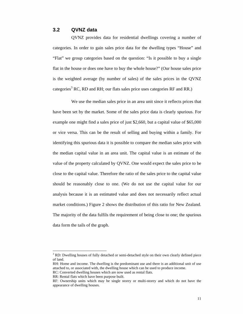
We use the median sales price in an area unit since it reflects prices that

have been set by the market. Some of the sales price data is clearly spurious. For

example one might find a sales price of just $2,660, but a capital value of $65,000

or vice versa. This can be the result of selling and buying within a family. For

identifying this spurious data it is possible to compare the median sales price with

the median capital value in an area unit. The capital value is an estimate of the

value of the property calculated by QVNZ. One would expect the sales price to be

close to the capital value. Therefore the ratio of the sales price to the capital value

should be reasonably close to one. (We do not use the capital value for our

analysis because it is an estimated value and does not necessarily reflect actual

market conditions.) Figure 2 shows the distribution of this ratio for New Zealand.

The majority of the data fulfils the requirement of being close to one; the spurious

data form the tails of the graph.

3 RD: Dwelling houses of fully detached or semi-detached style on their own clearly defined piece of land. RH: Home and income. The dwelling is the predominant use and there is an additional unit of use attached to, or associated with, the dwelling house which can be used to produce income. RC: Converted dwelling houses which are now used as rental flats. RR: Rental flats which have been purpose built. RF: Ownership units which may be single storey or multi-storey and which do not have the appearance of dwelling houses.

12

Figure 2: Identifying spurious sale prices

0.1

.2.3

.4.5

.6.7

.8.9

1cu

mul

ativ

e

0 1 2 3 4 5sales price / capital value (2001)

Identifying spurious sales prices

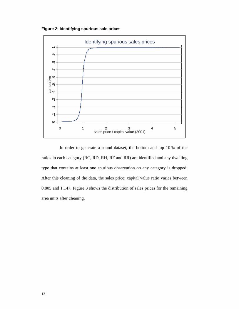
In order to generate a sound dataset, the bottom and top 10 % of the

ratios in each category (RC, RD, RH, RF and RR) are identified and any dwelling

type that contains at least one spurious observation on any category is dropped.

After this cleaning of the data, the sales price: capital value ratio varies between

0.805 and 1.147. Figure 3 shows the distribution of sales prices for the remaining

area units after cleaning.

13

Figure 3: Distribution of House Prices for New Zealand, 2001

020

0040

0060

00no

. of a

sses

smen

ts

0 100000 200000 300000 400000 500000 600000 700000Sales Price (median) 2001

Distribution of house prices after cleaning

3.3 Tenancy bond data An examination of the tenancy bond dataset indicates that it does not

contain obviously spurious observations. However we drop observations where

the owner may set rents that do not necessarily reflect market conditions. Hence

observations where Housing NZ or the Local Authority is the landlord are

dropped and only private landlords remain in the dataset. Furthermore, single

rooms are deleted from the dataset. Figure 4 shows the distribution of rents for the

remaining data.

14

Figure 4: Distribution of Rents for New Zealand, 2001

050

100

150

200

250

no o

f obs

erva

tions

0 100 200 300 400 500Rent per week (median)

Houses and Flats - average in area unitDistribution of rents

4 Relationship Between Rents & Prices This section examines the relationship between rents and prices for each

of houses and flats at aggregate level (i.e. aggregating all sized houses together

and aggregating all sized flats together). According to the theory in section 2,

rents are determined by prices and by expected capital gains. Higher expected

capital gains should result in a lower rent/price ratio. In order to illustrate the

validity of this model we initially conduct a simple two-step test.

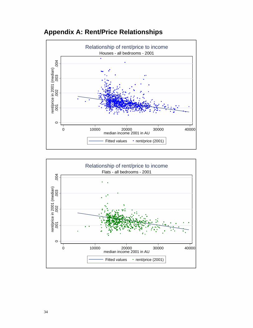
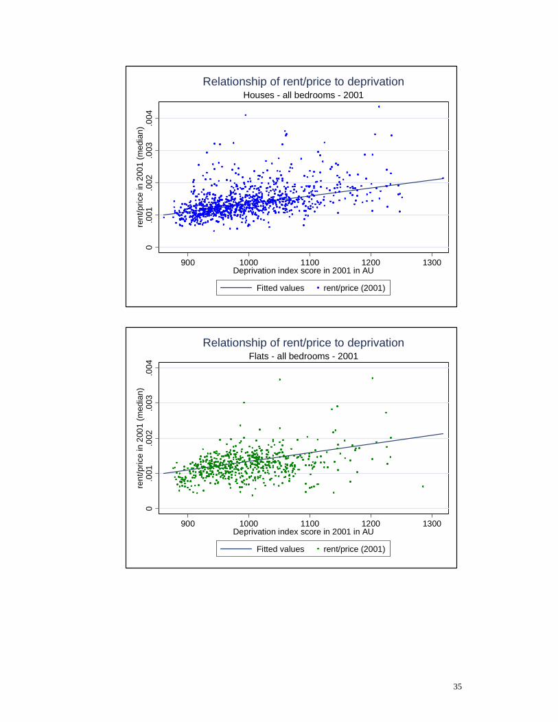
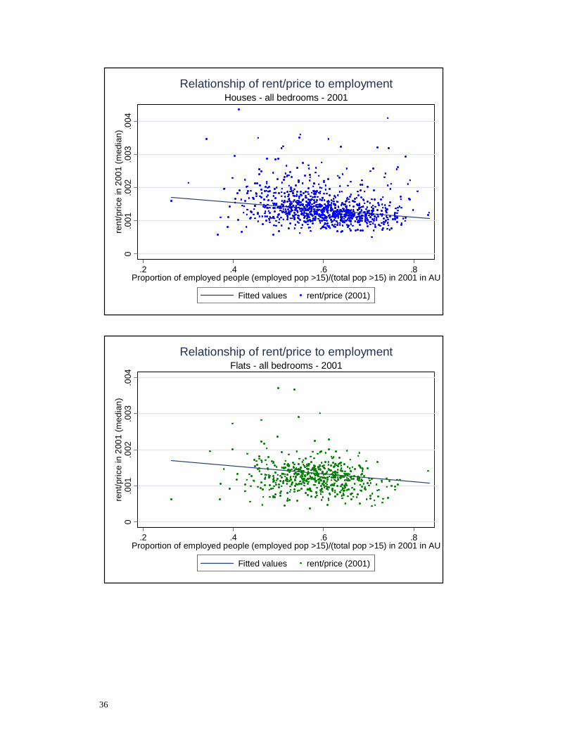
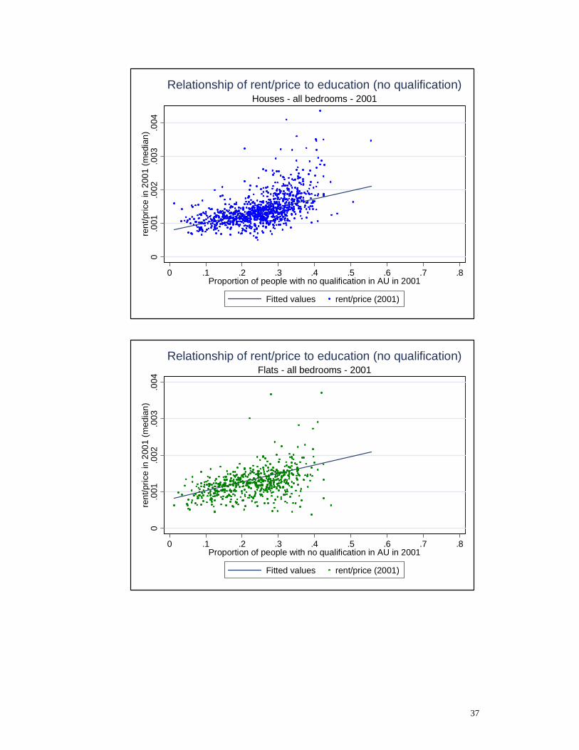
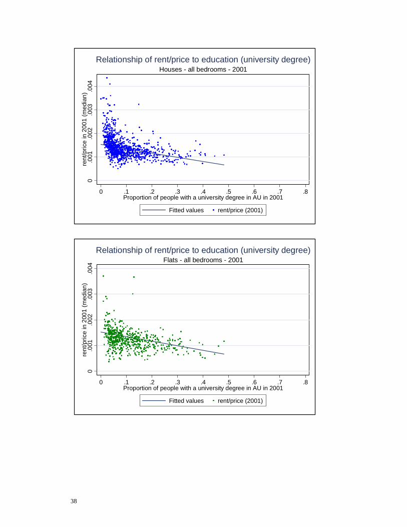
At first the rent/price-ratio for 2001 is correlated across AUs with

socio-economic variables hypothesised to influence the desirability of an area and

hence influence capital gains. In particular, we examine the relationship between

this ratio and each of income, deprivation, employment and two separate

15

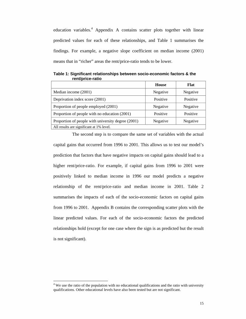
education variables.4 Appendix A contains scatter plots together with linear

predicted values for each of these relationships, and Table 1 summarises the

findings. For example, a negative slope coefficient on median income (2001)

means that in “richer” areas the rent/price-ratio tends to be lower.

Table 1: Significant relationships between socio-economic factors & the rent/price-ratio

House Flat

Median income (2001) Negative Negative

Deprivation index score (2001) Positive Positive

Proportion of people employed (2001) Negative Negative

Proportion of people with no education (2001) Positive Positive

Proportion of people with university degree (2001) Negative Negative All results are significant at 1% level.

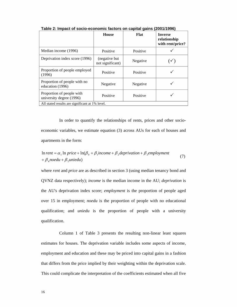
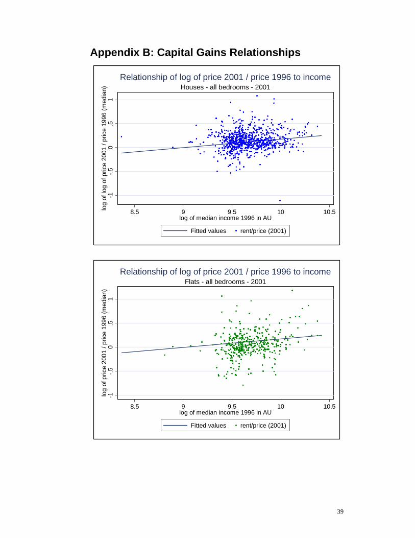
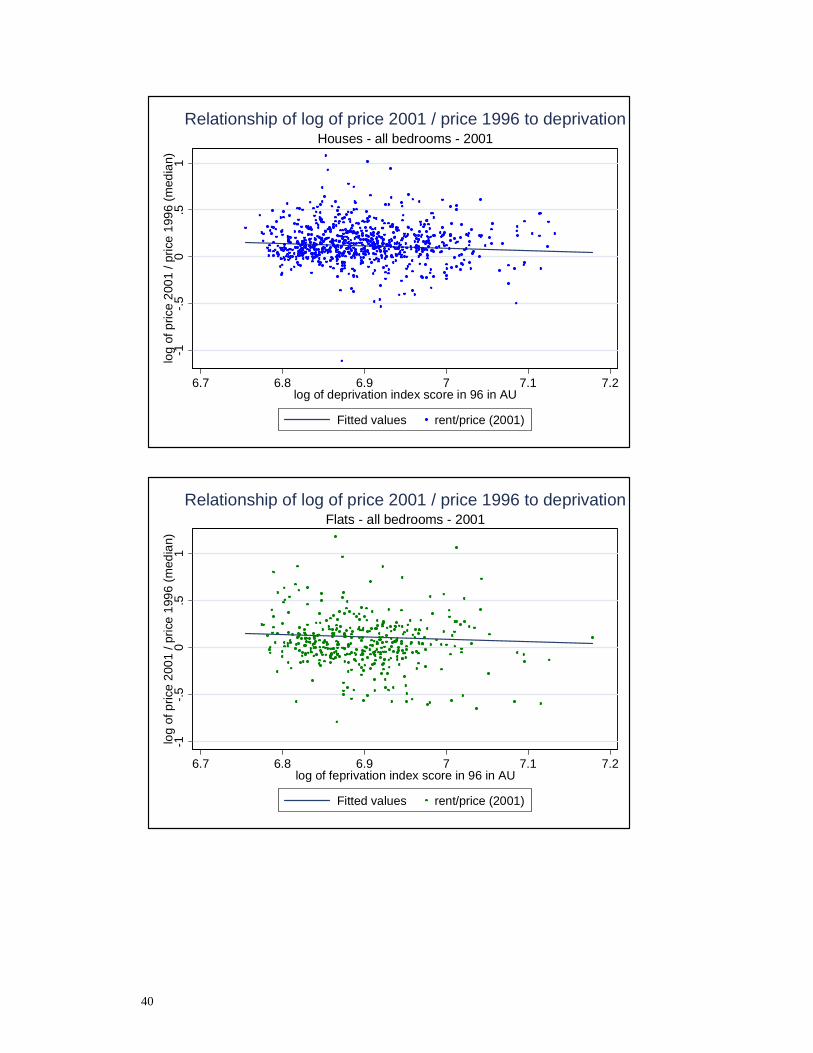
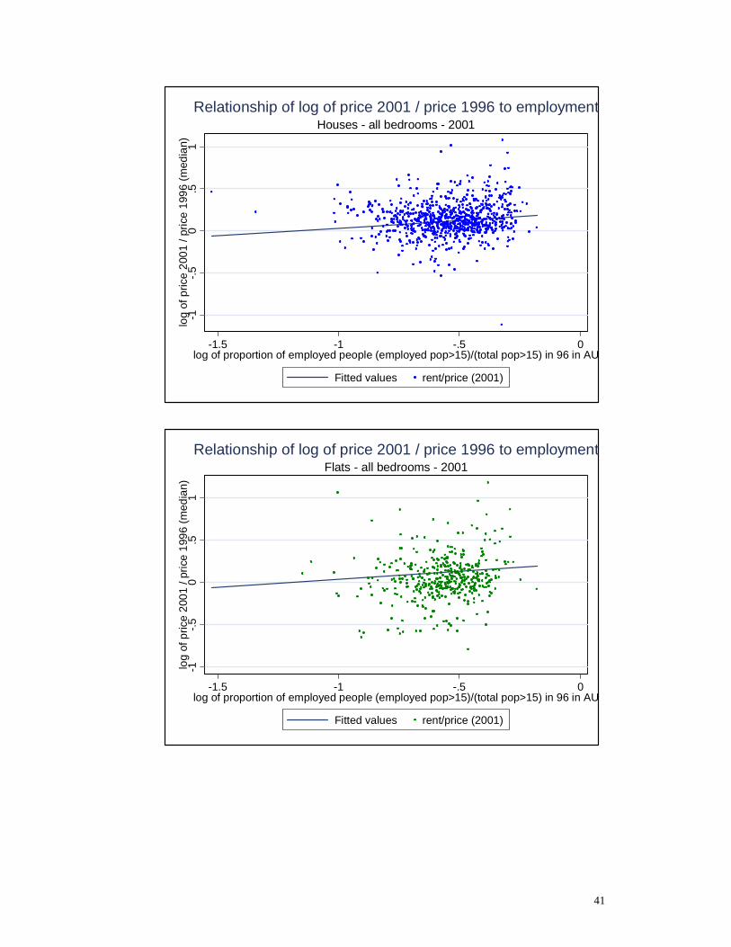
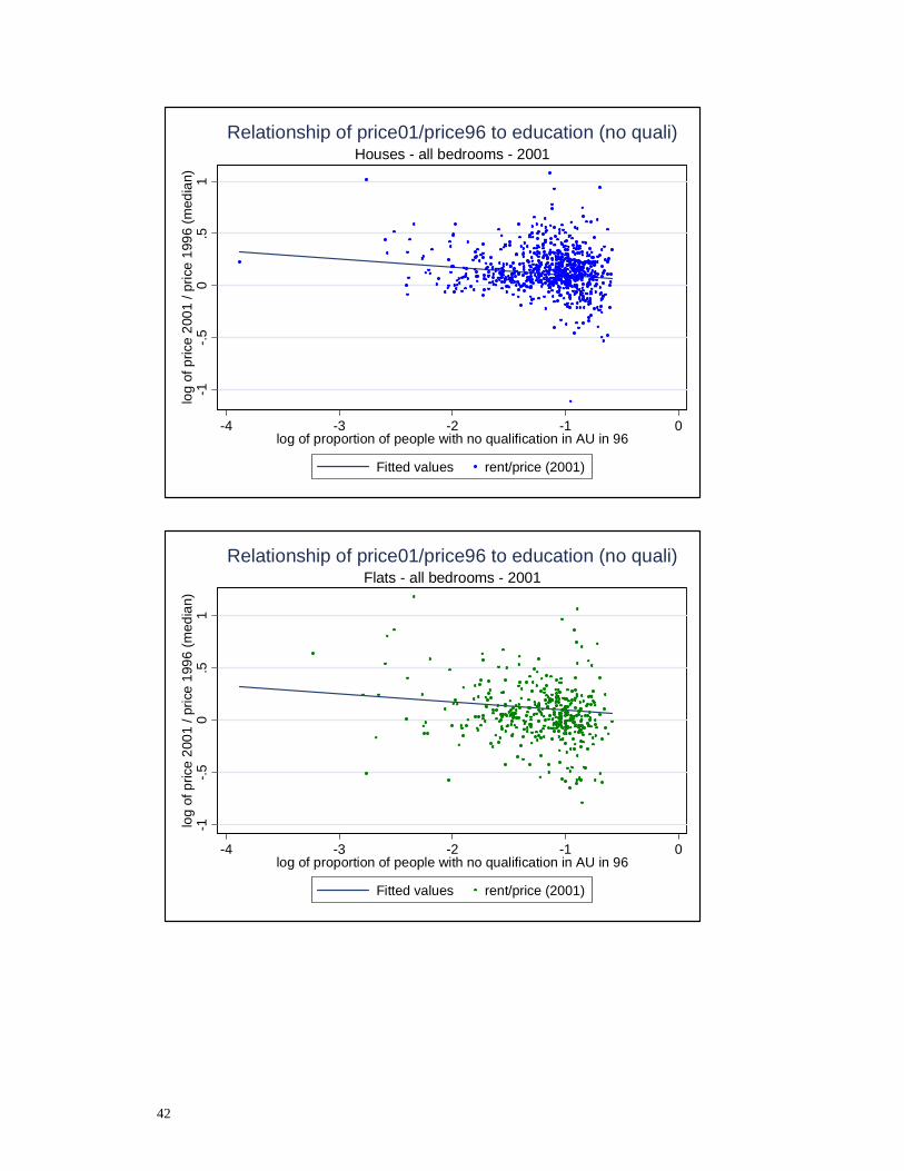
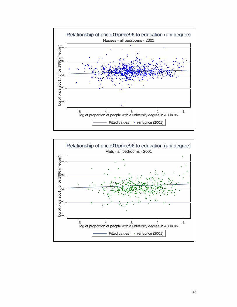
The second step is to compare the same set of variables with the actual

capital gains that occurred from 1996 to 2001. This allows us to test our model’s

prediction that factors that have negative impacts on capital gains should lead to a

higher rent/price-ratio. For example, if capital gains from 1996 to 2001 were

positively linked to median income in 1996 our model predicts a negative

relationship of the rent/price-ratio and median income in 2001. Table 2

summarises the impacts of each of the socio-economic factors on capital gains

from 1996 to 2001. Appendix B contains the corresponding scatter plots with the

linear predicted values. For each of the socio-economic factors the predicted

relationships hold (except for one case where the sign is as predicted but the result

is not significant).

4 We use the ratio of the population with no educational qualifications and the ratio with university qualifications. Other educational levels have also been tested but are not significant.

16

Table 2: Impact of socio-economic factors on capital gains (2001/1996) House Flat Inverse

relationship with rent/price?

Median income (1996) Positive Positive Deprivation index score (1996) (negative but

not significant) Negative ( )

Proportion of people employed (1996) Positive Positive

Proportion of people with no education (1996) Negative Negative

Proportion of people with university degree (1996) Positive Positive All stated results are significant at 1% level.

In order to quantify the relationships of rents, prices and other socio-

economic variables, we estimate equation (3) across AUs for each of houses and

apartments in the form:

)ln(lnln

54

32101

uniedunoeduemploymentndeprivatioincomepricerent

ββββββα

++++++=

(7)

where rent and price are as described in section 3 (using median tenancy bond and

QVNZ data respectively); income is the median income in the AU; deprivation is

the AU's deprivation index score; employment is the proportion of people aged

over 15 in employment; noedu is the proportion of people with no educational

qualification; and uniedu is the proportion of people with a university

qualification.

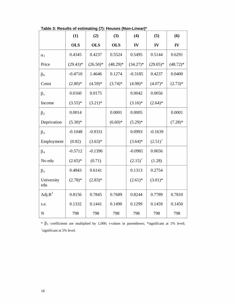
Column 1 of Table 3 presents the resulting non-linear least squares

estimates for houses. The deprivation variable includes some aspects of income,

employment and education and these may be priced into capital gains in a fashion

that differs from the price implied by their weighting within the deprivation scale.

This could complicate the interpretation of the coefficients estimated when all five

17

capital gains proxies are included. To test the robustness of our estimates to this

possibility, column 2 presents the results with deprivation omitted, while column

3 presents the results with deprivation included but with the remaining four capital

gains proxies excluded.

The results indicate that house prices are a major determinant of rents,

albeit with a coefficient of around one half rather than unity (we discuss possible

reasons for this further below). The socio-economic variables hypothesised to

influence capital gains are also important. Higher deprivation increases rents for a

given house price as indicated previously by the graphs. In addition, each of

income, employment and the two education variables impact significantly on rents

in at least one of the specifications.

18

Table 3: Results of estimating (7): Houses (Non-Linear)*

(1) (2) (3) (4) (5) (6)

OLS OLS OLS IV IV IV

α1 0.4345 0.4237 0.5524 0.5495 0.5144 0.6291

Price (29.43)* (26.50)* (48.29)* (34.27)* (29.05)* (48.72)*

β0 -0.4710 1.4646 0.1274 -0.3185 0.4237 0.0400

Const (2.80)* (4.59)* (3.74)* (4.98)* (4.07)* (2.73)*

β1 0.0160 0.0175 0.0042 0.0056

Income (3.55)* (3.21)* (3.16)* (2.64)*

β2 0.0014 0.0001 0.0005 0.0001

Deprivation (5.30)* (6.60)* (5.29)* (7.28)*

β3 -0.1048 -0.9331 0.0993 -0.1639

Employment (0.82) (3.63)* (3.64)* (2.51)+

β4 -0.5712 -0.1396 -0.0981 0.0656

No edu (2.65)* (0.71) (2.15)+ (1.28)

β5 0.4843 0.6141 0.1313 0.2754

University edu

(2.78)* (2.83)* (2.61)* (3.01)*

Adj.R2 0.8156 0.7845 0.7689 0.8244 0.7789 0.7810

s.e. 0.1332 0.1441 0.1490 0.1299 0.1459 0.1450

N 798 798 798 798 798 798

* β1 coefficients are multiplied by 1,000; t-values in parentheses; *significant at 1% level; +significant at 5% level.

19

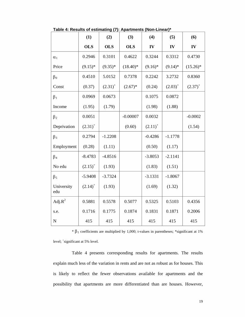
Table 4: Results of estimating (7): Apartments (Non-Linear)*

(1) (2) (3) (4) (5) (6)

OLS OLS OLS IV IV IV

α1 0.2946 0.3101 0.4622 0.3244 0.3312 0.4730

Price (9.15)* (9.35)* (18.40)* (9.16)* (9.14)* (15.26)*

β0 0.4510 5.0152 0.7378 0.2242 3.2732 0.8360

Const (0.37) (2.31)+ (2.67)* (0.24) (2.03)+ (2.37)+

β1 0.0969 0.0673 0.1075 0.0872

Income (1.95) (1.79) (1.98) (1.88)

β2 0.0051 -0.00007 0.0032 -0.0002

Deprivation (2.31)+ (0.60) (2.11)+ (1.54)

β3 0.2794 -1.2208 -0.4286 -1.1778

Employment (0.28) (1.11) (0.50) (1.17)

β4 -8.4783 -4.8516 -3.8053 -2.1141

No edu (2.15)+ (1.93) (1.83) (1.51)

β5 -5.9408 -3.7324 -3.1331 -1.8067

University edu

(2.14)+ (1.93) (1.69) (1.32)

Adj.R2 0.5881 0.5578 0.5077 0.5325 0.5103 0.4356

s.e. 0.1716 0.1775 0.1874 0.1831 0.1871 0.2006

N 415 415 415 415 415 415

* β1 coefficients are multiplied by 1,000; t-values in parentheses; *significant at 1%

level; +significant at 5% level.

Table 4 presents corresponding results for apartments. The results

explain much less of the variation in rents and are not as robust as for houses. This

is likely to reflect the fewer observations available for apartments and the

possibility that apartments are more differentiated than are houses. However,

20

some similarities with the house results are apparent, particularly the "low", but

significant, coefficient on the price variable.

In each case, there is the potential for endogeneity of the regressors to

cause inconsistent estimates. Our theory suggests that rents, prices and capital

gains expectations are formed simultaneously. Further, each of the socio-

economic variables could be affected by the level of rents (e.g. the proportion of

the population in an area with no formal education might be partially determined,

through migration and location choices, by rents charged in that area). To test the

sensitivity of our results to potential simultaneity bias, we re-estimate each of the

three equations for houses and for apartments using instrumental variables (IV).

We replace each of the six regressors with their 1996 values and present the

estimation results as columns 4 - 6 in the two tables.

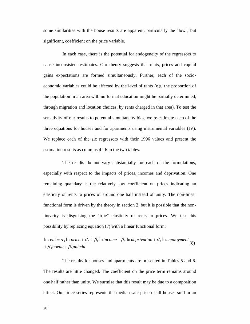
The results do not vary substantially for each of the formulations,

especially with respect to the impacts of prices, incomes and deprivation. One

remaining quandary is the relatively low coefficient on prices indicating an

elasticity of rents to prices of around one half instead of unity. The non-linear

functional form is driven by the theory in section 2, but it is possible that the non-

linearity is disguising the "true" elasticity of rents to prices. We test this

possibility by replacing equation (7) with a linear functional form:

uniedunoeduemploymentndeprivatioincomepricerent

54

32101 lnlnlnlnlnββ

ββββα++

++++=(8)

The results for houses and apartments are presented in Tables 5 and 6.

The results are little changed. The coefficient on the price term remains around

one half rather than unity. We surmise that this result may be due to a composition

effect. Our price series represents the median sale price of all houses sold in an

21

AU in a particular year. This includes rented and owner-occupied dwellings. In a

low price area, it is likely that the rental stock and owner-occupied stock are of

similar quality; hence the observed aggregate price is an adequate proxy for the

price of rental dwellings. By contrast, it is quite conceivable in high price areas

that relatively low quality houses within the area will tend to be rented. If this is

the case, the relationship of rentals prices to aggregate prices will be upward

sloping but with a coefficient of less than one. This relationship will then be

reflected in our estimates and, if the theoretical relationship outlined in section 2

holds, the elasticity of rents to prices would reflect this composition effect.

Without additional data, we cannot determine whether the estimated coefficient(s)

represent this effect or some other factor.5

5 Future work, using panel data, could identify if composition is having an effect on the estimates, provided composition effects are stable over time.

22

Table 5: Results of estimating (8): Houses (Linear)*

(1) (2) (3) (4) (5) (6)

OLS OLS OLS IV IV IV

α1 0.4311 0.4291 0.5528 0.5486 0.5217 0.6300

Price (28.75)* (26.26)* (48.31)* (34.61)* (29.40)* (48.88)*

β0 -12.310 -2.0285 -5.0344 -15.7505 -2.4866 -6.8125

Const (13.00)* (4.28)* (7.84)* (15.88)* (5.42)* (9.87)*

β1 0.2684 0.2021 0.2251 0.1484

Income (5.86)* (4.07)* (5.15)* (3.03)*

β2 1.4384 0.5402 1.8252 0.6786

Deprivation (12.23)* (6.57)* (14.67)* (7.82)*

β3 -0.0266 -0.3671 0.1912 -0.1653

Employment (0.40) (5.64)* (3.45)* (2.94)*

β4 -0.6460 -0.1387 -0.3743 0.1490

No edu (4.53)* (0.93) (3.30)* (1.23)

β5 0.4044 0.5368 0.4618 0.6679

University edu

(2.99)* (3.65)* (3.24)* (4.18)*

Adj.R2 0.8149 0.7802 0.7689 0.8245 0.7771 0.7813

s.e. 0.1335 0.1455 0.1492 0.1300 0.1465 0.1451

N 798 798 798 798 798 798

* t-values in parentheses; *significant at 1% level; +significant at 5% level.

.

23

Table 6: Results of estimating (8): Apartments (Linear)*

(1) (2) (3) (4) (5) (6)

OLS OLS OLS IV IV IV

α1 0.2905 0.3041 0.4610 0.3280 0.3302 0.4697

Price (9.00)* (9.12)* (18.23)* (9.09)* (8.95)* (15.01)*

β0 -10.2411 -1.5993 0.4206 -10.7423 -2.9959 2.4496

Const (5.97)* (2.09)+ (0.34) (5.57)* (3.41)* (1.82)

β1 0.4455 0.3380 0.5365 0.4437

Income (5.52)* (4.16)* (5.94)* (4.93)*

β2 1.1562 -0.1166 1.0277 -0.4221

Deprivation (5.58)* (0.75) (4.48)* (2.53)+

β3 -0.0697 -0.2295 -0.0987 -0.2221

Employment (0.58) (1.91) (0.79) (1.77)

β4 -1.7399 -1.2381 -1.0592 -0.6714

No edu (6.62)* (4.84)* (4.39)* (2.92)*

β5 -1.1039 -0.8565 -0.7548 -0.4848

University edu

(4.83)* (3.69)* (2.81)* (1.81)

Adj.R2 0.5905 0.5603 0.5079 0.5308 0.5088 0.4366

s.e. 0.1709 0.1771 0.1874 0.1830 0.1872 0.2005

N 415 415 415 415 415 415

* t-values in parentheses; *significant at 1% level; +significant at 5% level.

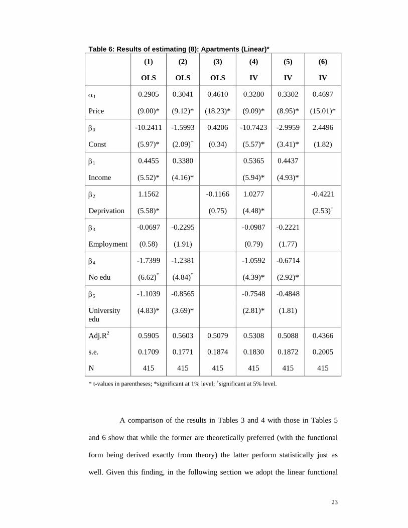
A comparison of the results in Tables 3 and 4 with those in Tables 5

and 6 show that while the former are theoretically preferred (with the functional

form being derived exactly from theory) the latter perform statistically just as

well. Given this finding, in the following section we adopt the linear functional

24

form in estimating the determinants of rents for additional bedrooms across areas.

This is particularly useful given the added coefficient non-linearities that we wish

to test in that work.

5 Rental Costs of Extra Bedrooms Having examined the determinants of rents at the aggregate (all

bedroom) level we turn now to estimating the cost of additional bedrooms across

areas. For reasons of space, and given the relative lack of observations on

apartments, we restrict our attention here to houses, although preliminary work

shows apartments to follow similar pricing principles. We omit five bedroom

houses owing to the small number of observations for that group.

We use equation (5) from section 2 as our basis. We express it in a

slightly different, but equivalent, form by including a constant term plus three

intercept dummies for 2, 3 and 4 bedroom houses; similarly, we include lnPi plus

three slope dummies representing interactions between the number of bedrooms

and the price. Given the results in section 4 showing little difference between the

linear and non-linear versions, we linearise the equation and estimate the form

shown in (9):

ln ijR = δ0 + Σ 42=j δjDj + ε0ln iP + Σ 4

2=j εjDj.ln iP + Σ 51=k βk kiY (9)

where Y1 is ln income

Y2 is ln deprivation

Y3 is ln employment

Y4 is noedu

Y5 is uniedu

Each of the variables is as defined in section 4. In keeping with section

4, we estimate the equations both with OLS on 2001 data and with IV using the

1996 data to instrument for each of the regressors. The results are shown in Table

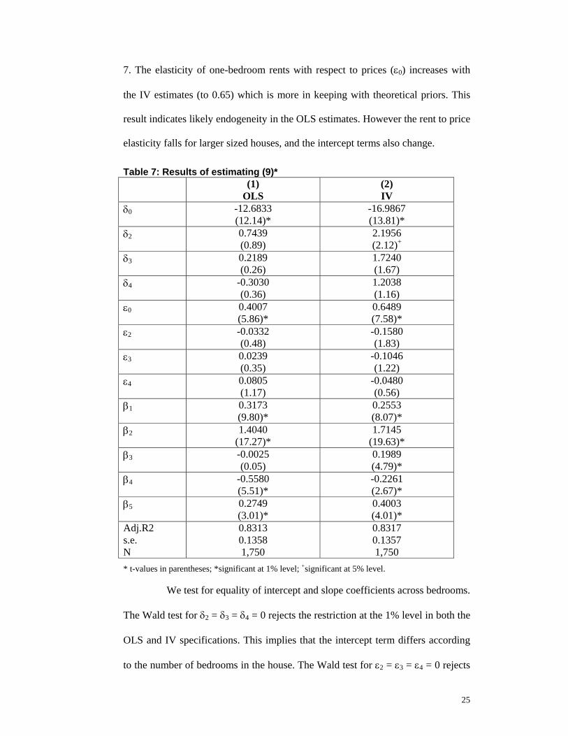
25

7. The elasticity of one-bedroom rents with respect to prices (ε0) increases with

the IV estimates (to 0.65) which is more in keeping with theoretical priors. This

result indicates likely endogeneity in the OLS estimates. However the rent to price

elasticity falls for larger sized houses, and the intercept terms also change.

Table 7: Results of estimating (9)* (1)

OLS (2) IV

δ0 -12.6833 (12.14)*

-16.9867 (13.81)*

δ2 0.7439 (0.89)

2.1956 (2.12)+

δ3 0.2189 (0.26)

1.7240 (1.67)

δ4 -0.3030 (0.36)

1.2038 (1.16)

ε0 0.4007 (5.86)*

0.6489 (7.58)*

ε2 -0.0332 (0.48)

-0.1580 (1.83)

ε3 0.0239 (0.35)

-0.1046 (1.22)

ε4 0.0805 (1.17)

-0.0480 (0.56)

β1 0.3173 (9.80)*

0.2553 (8.07)*

β2 1.4040 (17.27)*

1.7145 (19.63)*

β3 -0.0025 (0.05)

0.1989 (4.79)*

β4 -0.5580 (5.51)*

-0.2261 (2.67)*

β5 0.2749 (3.01)*

0.4003 (4.01)*

Adj.R2 s.e. N

0.8313 0.1358 1,750

0.8317 0.1357 1,750

* t-values in parentheses; *significant at 1% level; +significant at 5% level.

We test for equality of intercept and slope coefficients across bedrooms.

The Wald test for δ2 = δ3 = δ4 = 0 rejects the restriction at the 1% level in both the

OLS and IV specifications. This implies that the intercept term differs according

to the number of bedrooms in the house. The Wald test for ε2 = ε3 = ε4 = 0 rejects

26

this restriction at the 1% level in both the OLS and IV specifications. Thus the

slope coefficients on the price term also differ according to the number of

bedrooms. Finally, the joint set of restrictions that δ2 = δ3 = δ4 = ε2 = ε3 = ε4 = 0 is

rejected at the 1% level in both the OLS and IV specifications.

The results therefore indicate that not only does the average rent of

houses in an area increase with average sale prices in an area, but the rental price

of additional bedrooms also varies according to the price of houses. To give an

indication of how material each of the effects is, we calculate the estimated

weekly rent for each sized house (where R1, R2, R3, R4 correspond to the

estimated weekly rents for 1, 2, 3 and 4 bedroom houses respectively). The

estimates use mean values for each variable in 2001 and 1996 and use the

corresponding estimates from columns 1 and 2 of Table 7. The results are

presented in the first row of Tables 8 and 9 using the OLS and IV estimates

respectively. The last three columns of each table show the price of an additional

room (e.g. R2-R1 is the rent for a 2-bedroom house less the rent for a 1-bedroom

house). The estimated rents are very similar using the two sets of estimates.

27

Table 8: Effect of Variables on Rents ($ per week) - OLS (2001 data)* R1 R2 R3 R4 R2-R1 R3-R2 R4-R3

All @ means 119.40 169.28 197.56 230.02 49.88 28.28 32.46 Price: - 1SD 97.41 140.46 159.23 180.13 43.05 18.77 20.89Income: - 1SD 110.60 156.80 183.00 213.07 46.21 26.20 30.07Deprivation: - 1SD 132.03 187.19 218.47 254.36 55.16 31.27 35.89All (ex.Price): -1 SD 114.13 161.81 188.84 219.87 47.68 27.03 31.02All: -1SD 93.07 134.20 152.13 172.09 41.13 17.93 19.96All: +1SD 153.38 213.82 256.90 307.85 60.44 43.08 50.95All variable changes, other than the last row, are "for the worse"; i.e. a decrease in price, income, employment, university qualifications; and an increase in deprivation and no educational qualifications. Changes in the last row all "for the better". Table 9: Effect of Variables on Rents ($ per week) - IV (1996 data)*

R1 R2 R3 R4 R2-R1 R3-R2 R4-R3 All @ means 120.91 169.30 197.99 229.12 48.40 28.69 31.13 Price: - 1SD 89.70 135.08 154.14 173.79 45.38 19.06 19.65Income: - 1SD 114.22 159.95 187.05 216.46 45.72 27.10 29.41Deprivation: - 1SD 136.01 190.45 222.72 257.74 54.44 32.27 35.02All (ex.Price): -1 SD 118.50 165.93 194.05 224.56 47.43 28.12 30.51All: -1SD 87.92 132.39 151.07 170.33 44.47 18.68 19.26All: +1SD 166.22 216.44 259.40 308.12 50.22 42.97 48.71All variable changes, other than the last row, are "for the worse"; i.e. a decrease in price, income, employment, university qualifications; and an increase in deprivation and no educational qualifications. Changes in the last row all "for the better".

The second row of each table shows the rents for different sized houses

where house prices are reduced one standard deviation below their mean in 2001

and 1996 respectively. In 2001, this means reducing the house price from the

mean of $148,227 to $89,089, while in 1996, it means reducing the house price

from $128,695 to $81,244. The one standard deviation reductions are of different

sizes in the two years because of different distributions in the data, so the results

are not directly comparable across the two data sets. They are nevertheless

qualitatively similar; henceforth we discuss just the preferred IV (Table 9) results

unless otherwise specified. Rents, as may be expected, are reduced across the

board. More pertinent to the questions posed at the outset of this study is the

sizeable difference in the cost of an extra bedroom, especially for larger houses.

The cost of four bedrooms relative to two bedrooms falls from $59.82 to $38.71

per week (a fall of $10.65 per extra bedroom) whereas the cost of the second

28

bedroom relative to the first falls by only $3.02. Thus rents for larger houses tend

to be much cheaper in lower price areas relative to high price areas than is the

case with smaller houses.

Rows 3 and 4 show the effects of a one standard deviation reduction in

income, ceteris paribus, and a one standard deviation "worsening" in deprivation

(i.e. an increase in deprivation). A fall in incomes is reflected in lower rents while

greater deprivation leads to a rise in rents. The latter effect is particularly marked:

a one standard deviation worsening in deprivation is associated with a 12.5%

increase in rents across the board. This effect is theoretically associated with

lower capital gains expectations in more deprived areas.

It would, however, be unusual to see deprivation or income change in

isolation from other variables. Row 5 indicates the estimated rents for different

sized houses if all variables other than house prices were to worsen by one

standard deviation. In this case, the effects are more or less offsetting, and rents

are 98% of their mean level (using 1996 data; 95.6% using 2001 data). If prices

are also reduced by one standard deviation (row 6), the price effect dominates.

The cost of a third and a fourth bedroom is each around $19 per week, compared

with a cost of around $30 for each of the third and fourth bedroom when all

variables are at their means.

To further emphasise this contrast in the cost of extra bedrooms as price

and other variables change across areas, the last row increases all variables by one

standard deviation. Comparing the last two rows shows a realistic divergence in

rents for different sized houses between "rich" and "poor" suburbs. In rich

suburbs, not only are rents much higher, but also the price of each additional

bedroom stays in a range of $42 - $51 per week. By contrast, in poor suburbs, the

29

price of a second bedroom is in the same range, but the price of third and fourth

bedrooms falls to around $19 each.

The estimates presented above allow for socio-economic influences

such as deprivation to impact on rents in an area, but that specification does not

allow these influences to impact on the price of additional bedrooms across

different areas. To examine whether socio-economic influences impact on the

pricing of additional bedrooms, we interacted each of the income and deprivation

terms with the intercept and price terms as in (6a) and (6b) of section 2. We then

tested whether these interaction effects were significant with Wald tests. Each of

the interactions of deprivation with intercept and slope terms was not significantly

different from zero, and almost all income interactions were similarly

insignificant. (The only significant effect for the latter occurred for 1-bedroom

houses, but the effect was small.) We therefore do not report these results here.

6 Implications Our results are noteworthy in a number of respects. First, the rental

market appears to be efficient in the sense that areas with high expected capital

gains have lower rental yields than areas with low expected capital gains. This

finding is based on an assumption that capital gains expectations are formed in a

forward-looking manner based on latest information, using influences seen to be

important in determining past capital gains.

We show that high levels of deprivation are associated with low capital

gains expectations; in other words, deprived areas are expected to remain in the

doldrums, while areas of low deprivation are expected to outperform. Thus more

30

deprived areas have higher rent to price ratios than do less deprived areas. While

this may seem "unfair" for renters in more deprived areas, it is a natural

consequence of landlords (and house sellers) seeking the same return across all

areas when investing in (and selling) rental housing.

Overall, the influences on expectations are complex, reflecting income,

employment and education outcomes specifically, as well as overall deprivation.

Accounting for all these effects, the main determinant of rents in an area is house

prices in that area.

Our second major finding is that the relative rents of different sized

houses is crucially dependent on the level of house prices. Areas with low house

prices tend to have more compressed relativities between rents of large and small

houses than is the case with high house price areas (both in relative and absolute

terms).

This latter finding is important when considering housing in a social

policy context. After accounting for other influences, the effect of this

compression will be to induce larger families to locate in lower priced areas and

smaller families to locate in higher priced areas. On the assumption that children

are more likely to live in larger than average households, the effect is to group

households with children together in lower priced areas (over and above any life-

cycle affordability effects). This grouping may have certain social capital benefits

(e.g. through the grouping of households with shared interests) but it may also

have negative social consequences. In particular, it may place added stress on

resources required to service children and families in poorer (lower priced) areas.

If provision of such services fails to meet the more intensive demand, negative

31

consequences can emerge (e.g. through inadequate child-care, schooling, health

services, parks, etc).

Further, there may be employment and other social and environmental

consequences of this compression. Larger families may choose to locate in low

priced areas, but the low prices may reflect lack of job prospects (e.g. in some

rural or semi-rural locations). Rental costs of larger houses may therefore act to

increase mis-match between jobs and potential workforce participants - especially

those with families - across the country. Alternatively, people may locate to lower

priced areas, but with long commute times to available work, placing greater

pressure on transport links and energy use.

While these effects may each be important, potential policy responses

have to be considered with care. Policies to subsidise housing can be capitalised

into the price (and/or the rent) with benefits accruing primarily to the existing

owner, and not necessarily to the recipient of the subsidy. Policy responses that

ensure services are up to scratch in areas with larger families help address the

negative social impacts that may arise from the grouping together of such

households, but will also tend to be reflected (through pricing of amenity values)

in house prices. Policies to provide income relief to larger households have less of

a distortionary effect on the housing market but have other complications, not

least of which is fiscal cost and hence the overall burden of taxation.

Encouraging home ownership is often viewed as a policy with positive

outcomes both socially and for more disadvantaged people that become house

owners. However, our theoretical framework and empirical results indicate that

care must be taken with such a policy initiative. Encouraging home ownership

amongst renters in areas with high rents (relative to prices) may have the effect of

32

inducing lower income families to make housing investments in areas with low

prospective capital gains. This outcome could, in turn, perpetuate their relative

disadvantage.

Given the complexities associated with housing policy, it is likely that

some mixture of policy responses will be appropriate. Whatever the responses, it

is important to ensure that negative social effects arising from concentration of

large families in relatively cheap rental accommodation is minimised if long term

disadvantage associated with housing conditions is to be avoided.

33

References Brealey, R. and S. Myers. 2003. Principles of Corporate Finance, seventh ed., New York:

McGraw-Hill.

Can, A. 1992. "Specification and Estimation of Hedonic Housing Price Models," Regional Science and Urban Economics, 22:3, pp. 453-74.

Capozza, Dennis R and Paul J. Seguin. 1996. "Expectations, Efficiency, and Euphoria in the Housing Market," Regional Science and Urban Economics, 26, pp. 369-86.

Crampton, Peter; Clare Salmond, Russell Kirkpatrick, R. Scarborough and Chris Skelly. 2000. Degrees of Deprivation in New Zealand: An Atlas of Socioeconomic Difference, Auckland: David Bateman.

DTZ Research. 2004. "Housing Costs and Affordability," Report prepared for the Centre for Housing Research Aotearoa New Zealand, DTZ Research, Wellington. Available online at http://www.chranz.co.nz/ Last accessed 12/5/05.

Dubin, R. A. 1992. "Spatial Autocorrelation and Neighbourhood Quality," Regional Science and Urban Economics, 22:3, pp. 433-52.

Grimes, Arthur and Andrew Aitken. 2004. "What's the Beef With House Prices?: Economic Shocks and Local Housing Markets," Motu Working Paper 04-08, Motu Economic and Public Policy Research, Wellington, New Zealand. Available online at http://www.motu.org.nz/motu_wp_series.htm.

Grimes, Arthur; Suzi Kerr and Andrew Aitken. 2003. "Housing and Economic Adjustment," Motu Working Paper 03-09, Motu Economic and Public Policy Trust, Wellington, New Zealand. Available online at http://www.motu.org.nz/motu_wp_series.htm.

Meen, Geoffrey P. 2001. Modelling Spatial Housing Markets: Theory, Analysis and Policy, Boston: Kluwer Academic Publishers.

Smith, K. S. and R. Fraser. 2004. "National Landlords Survey: Preliminary Analysis of the Data," Centre for Research, Evaluation and Social Assessment, Wellington, New Zealand.

34

Appendix A: Rent/Price Relationships

0.0

01.0

02.0

03.0

04re

nt/p

rice

in 2

001

(med

ian)

0 10000 20000 30000 40000median income 2001 in AU

Fitted values rent/price (2001)

Houses - all bedrooms - 2001Relationship of rent/price to income

0.0

01.0

02.0

03.0

04re

nt/p

rice

in 2

001

(med

ian)

0 10000 20000 30000 40000median income 2001 in AU

Fitted values rent/price (2001)

Flats - all bedrooms - 2001Relationship of rent/price to income

35

0.0

01.0

02.0

03.0

04re

nt/p

rice

in 2

001

(med

ian)

900 1000 1100 1200 1300Deprivation index score in 2001 in AU

Fitted values rent/price (2001)

Houses - all bedrooms - 2001Relationship of rent/price to deprivation

0.0

01.0

02.0

03.0

04re

nt/p

rice

in 2

001

(med

ian)

900 1000 1100 1200 1300Deprivation index score in 2001 in AU

Fitted values rent/price (2001)

Flats - all bedrooms - 2001Relationship of rent/price to deprivation

36

0.0

01.0

02.0

03.0

04re

nt/p

rice

in 2

001

(med

ian)

.2 .4 .6 .8Proportion of employed people (employed pop >15)/(total pop >15) in 2001 in AU

Fitted values rent/price (2001)

Houses - all bedrooms - 2001Relationship of rent/price to employment

0.0

01.0

02.0

03.0

04re

nt/p

rice

in 2

001

(med

ian)

.2 .4 .6 .8Proportion of employed people (employed pop >15)/(total pop >15) in 2001 in AU

Fitted values rent/price (2001)

Flats - all bedrooms - 2001Relationship of rent/price to employment

37

0.0

01.0

02.0

03.0

04re

nt/p

rice

in 2

001

(med

ian)

0 .1 .2 .3 .4 .5 .6 .7 .8Proportion of people with no qualification in AU in 2001

Fitted values rent/price (2001)

Houses - all bedrooms - 2001Relationship of rent/price to education (no qualification)

0.0

01.0

02.0

03.0

04re

nt/p

rice

in 2

001

(med

ian)

0 .1 .2 .3 .4 .5 .6 .7 .8Proportion of people with no qualification in AU in 2001

Fitted values rent/price (2001)

Flats - all bedrooms - 2001Relationship of rent/price to education (no qualification)

38

0.0

01.0

02.0

03.0

04re

nt/p

rice

in 2

001

(med

ian)

0 .1 .2 .3 .4 .5 .6 .7 .8Proportion of people with a university degree in AU in 2001

Fitted values rent/price (2001)

Houses - all bedrooms - 2001Relationship of rent/price to education (university degree)

0.0

01.0

02.0

03.0

04re

nt/p

rice

in 2

001

(med

ian)

0 .1 .2 .3 .4 .5 .6 .7 .8Proportion of people with a university degree in AU in 2001

Fitted values rent/price (2001)

Flats - all bedrooms - 2001Relationship of rent/price to education (university degree)

39

Appendix B: Capital Gains Relationships

-1-.5

0.5

1lo

g of

log

of p

rice

2001

/ pr

ice

1996

(med

ian)

8.5 9 9.5 10 10.5log of median income 1996 in AU

Fitted values rent/price (2001)

Houses - all bedrooms - 2001Relationship of log of price 2001 / price 1996 to income

-1-.5

0.5

1lo

g of

pric

e 20

01 /

pric

e 19

96 (m

edia

n)

8.5 9 9.5 10 10.5log of median income 1996 in AU

Fitted values rent/price (2001)

Flats - all bedrooms - 2001Relationship of log of price 2001 / price 1996 to income

40

-1-.5

0.5

1lo

g of

pric

e 20

01 /

pric

e 19

96 (m

edia

n)

6.7 6.8 6.9 7 7.1 7.2log of deprivation index score in 96 in AU

Fitted values rent/price (2001)

Houses - all bedrooms - 2001Relationship of log of price 2001 / price 1996 to deprivation

-1-.5

0.5

1lo

g of

pric

e 20

01 /

pric

e 19

96 (m

edia

n)

6.7 6.8 6.9 7 7.1 7.2log of feprivation index score in 96 in AU

Fitted values rent/price (2001)

Flats - all bedrooms - 2001Relationship of log of price 2001 / price 1996 to deprivation

41

-1-.5

0.5

1lo

g of

pric

e 20

01 /

pric

e 19

96 (m

edia

n)

-1.5 -1 -.5 0log of proportion of employed people (employed pop>15)/(total pop>15) in 96 in AU

Fitted values rent/price (2001)

Houses - all bedrooms - 2001Relationship of log of price 2001 / price 1996 to employment

-1-.5

0.5

1lo

g of

pric

e 20

01 /

pric

e 19

96 (m

edia

n)

-1.5 -1 -.5 0log of proportion of employed people (employed pop>15)/(total pop>15) in 96 in AU

Fitted values rent/price (2001)

Flats - all bedrooms - 2001Relationship of log of price 2001 / price 1996 to employment

42

-1-.5

0.5

1lo

g of

pric

e 20

01 /

pric

e 19

96 (m

edia

n)

-4 -3 -2 -1 0log of proportion of people with no qualification in AU in 96

Fitted values rent/price (2001)

Houses - all bedrooms - 2001Relationship of price01/price96 to education (no quali)

-1-.5

0.5

1lo

g of

pric

e 20

01 /

pric

e 19

96 (m

edia

n)

-4 -3 -2 -1 0log of proportion of people with no qualification in AU in 96

Fitted values rent/price (2001)

Flats - all bedrooms - 2001Relationship of price01/price96 to education (no quali)

43

-1-.5

0.5

1lo

g of

pric

e 20

01 /

pric

e 19

96 (m

edia

n)

-5 -4 -3 -2 -1log of proportion of people with a university degree in AU in 96

Fitted values rent/price (2001)

Houses - all bedrooms - 2001Relationship of price01/price96 to education (uni degree)

-1-.5

0.5

1lo

g of

pric

e 20

01 /

pric

e 19

96 (m

edia

n)

-5 -4 -3 -2 -1log of proportion of people with a university degree in AU in 96

Fitted values rent/price (2001)

Flats - all bedrooms - 2001Relationship of price01/price96 to education (uni degree)

44

Motu Working Paper Series

05–01. Maré, David C., “Indirect Effects of Active Labour Market Policies”.

04–12. Dixon, Sylvia and David C Maré, “Understanding Changes in Maori Incomes and Income Inequality 1997-2003”.

04–11. Grimes, Arthur, “New Zealand: A Typical Australasian Economy?”

04–10. Hall, Viv and C. John McDermott, “Regional business cycles in New Zealand: Do they exist? What might drive them?”

04–09. Grimes, Arthur, Suzi Kerr and Andrew Aitken, “Bi-Directional Impacts of Economic, Social and Environmental changes and the New Zealand Housing Market”.

04–08. Grimes, Arthur, Andrew Aitken, “What’s the Beef with House Prices? Economic Shocks and Local Housing Markets”.

04–07. McMillan, John, “Quantifying Creative Destruction: Entrepreneurship and Productivity in New Zealand”.

04–06. Maré, David C and Isabelle Sin, “Maori Incomes: Investigating Differences Between Iwi”

04–05. Kerr, Suzi, Emma Brunton and Ralph Chapman, “Policy to Encourage Carbon Sequestration in Plantation Forests”.

04–04. Maré, David C, “What do Endogenous Growth Models Contribute?”

04–03. Kerr, Suzi, Joanna Hendy, Shuguang Liu and Alexander S.P. Pfaff, “Uncertainty and Carbon Policy Integrity”.

04–02. Grimes, Arthur, Andrew Aitken and Suzi Kerr, “House Price Efficiency: Expectations, Sales, Symmetry”.

04–01. Kerr, Suzi; Andrew Aitken and Arthur Grimes, “Land Taxes and Revenue Needs as Communities Grow and Decline: Evidence from New Zealand”.

03–19. Maré, David C, “Ideas for Growth?”.

03–18. Fabling, Richard and Arthur Grimes, “Insolvency and Economic Development:Regional Variation and Adjustment”.

03–17. Kerr, Suzi; Susana Cardenas and Joanna Hendy, “Migration and the Environment in the Galapagos:An analysis of economic and policy incentives driving migration, potential impacts from migration control, and potential policies to reduce migration pressure”.

03–16. Hyslop, Dean R. and David C. Maré, “Understanding New Zealand’s Changing Income Distribution 1983–98: A Semiparametric Analysis”.

03–15. Kerr, Suzi, “Indigenous Forests and Forest Sink Policy in New Zealand”.

03–14. Hall, Viv and Angela Huang, “Would Adopting the US Dollar Have Led To Improved Inflation, Output and Trade Balances for New Zealand in the 1990s?”

03–13. Ballantyne, Suzie; Simon Chapple, David C. Maré and Jason Timmins, “Movement into and out of Child Poverty in New Zealand: Results from the Linked Income Supplement”.

03–12. Kerr, Suzi, “Efficient Contracts for Carbon Credits from Reforestation Projects”.

03–11. Lattimore, Ralph, “Long Run Trends in New Zealand Industry Assistance”.

03–10. Grimes, Arthur, “Economic Growth and the Size & Structure of Government: Implications for New Zealand”.

03–09. Grimes, Arthur; Suzi Kerr and Andrew Aitken, “Housing and Economic Adjustment”.

03–07. Maré, David C. and Jason Timmins, “Moving to Jobs”.

03–06. Kerr, Suzi; Shuguang Liu, Alexander S. P. Pfaff and R. Flint Hughes, “Carbon Dynamics and Land-Use Choices: Building a Regional-Scale Multidisciplinary Model”.

45

03–05. Kerr, Suzi, “Motu, Excellence in Economic Research and the Challenges of 'Human Dimensions' Research”.

03–04. Kerr, Suzi and Catherine Leining, “Joint Implementation in Climate Change Policy”.

03–03. Gibson, John, “Do Lower Expected Wage Benefits Explain Ethnic Gaps in Job-Related Training? Evidence from New Zealand”.

03–02. Kerr, Suzi; Richard G. Newell and James N. Sanchirico, “Evaluating the New Zealand Individual Transferable Quota Market for Fisheries Management”.

03–01. Kerr, Suzi, “Allocating Risks in a Domestic Greenhouse Gas Trading System”.

All papers are available online at http://www.motu.org.nz/motu_wp_series.htm