Regimes of biological invasion in a predator–prey system ... · Main equations We c onsider the...

Bulletin of Mathematical Biology 67 (2005) 637–661

www.elsevier.com/locate/ybulm

Regimes of biological invasion in a predator–preysystem with the Allee effect

Sergei Petrovskiia,b,∗, Andrew Morozova,b, Bai-Lian Lib

aShirshov Institute of Oceanology, Russian Academy of Science, Nakhimovsky Prospekt 36,Moscow 117218, Russia

bEcological Complexity and Modeling Laboratory, Department of Botany and Plant Sciences,University of California at Riverside, Riverside, CA 92521-0124, USA

Received 28 April 2004; accepted 15 September 2004

Abstract

Spatiotemporal dynamics of a predator–prey system is considered under the assumption that preygrowth is damped by the strong Allee effect. Mathematically, the model consists of two coupleddiffusion-reaction equations. The initial conditions are describedby functions of finite support whichcorresponds to invasion of exotic species. By means of extensive numerical simulations, we identifythe main scenarios of the system dynamics as related to biological invasion. We construct the mapsin the parameter space of the system with different domains corresponding to different invasionregimes and show that the impact of the Allee effect essentially increases the system spatiotemporalcomplexity. In particular, we show that, as a result of the interplay between the Allee effect andpredation, successful establishment of exotic species may not necessarily lead to geographical spreadand geographical spread does not always enhance regional persistence of invading species.© 2004 Society for Mathematical Biology. Published by Elsevier Ltd. All rights reserved.

1. Introduction

Biological invasion has been attracting considerable attention recently due to itsnumerous adverse effects on ecosystem dynamics and biodiversity (Hengeveld, 1989;

∗ Corresponding author at: Shirshov Institute of Oceanology, Russian Academy of Science, NakhimovskyProspekt 36, Moscow 117218, Russia.

E-mail address: [email protected] (S. Petrovskii).

0092-8240/$30 © 2004 Society for Mathematical Biology. Published by Elsevier Ltd. All rights reserved.doi:10.1016/j.bulm.2004.09.003

http://www.elsevier.com/locate/ybulm

638 S. Petrovskii et al. / Bulletin of Mathematical Biology 67 (2005) 637–661

Hastings, 1996; Shigesada and Kawasaki, 1997; Frantzen and van den Bosch, 2000; Keittet al., 2001; Owen and Lewis, 2001; Wang and Kot, 2001). Although a considerableprogress has been made during the last decade in understanding basic scenarios of speciesinvasion, many important issues have not been properly addressed yet. Comprehensiveidentification of factors that affect rates of invasion and patterns of species spread and canpotentially either enhance or hamper species invasion, is expected to open a possibilityof biological control and to result in effective invasive species management (Sakai et al.,2001; Fagan et al., 2002).

Biological invasion is known to have a few more or less clearly distinguishable stages[cf. Shigesada and Kawasaki (1997), Sakai et al. (2001)]. The first stage is introductionwhen a few organisms of an exotic species are brought, deliberately or unintentionally,into the given ecosystem. The second stage is establishment when the introduced species isgetting adapted to the new environmental conditions. The third stage is, in case the previoustwo have been successful and did not result in species extinction, the ‘geographical’ spreadwhen the exotic species invades new areas at the scale much larger compared to the domainwhere it was originally introduced. Later stages are relatedto the impact of the new specieson the native ecological community and, possibly, on human health and society.

Apparently, each stage has its own basic processes and specific problems. In this paper,we mainly focus on the spatiotemporal dynamics of the introduced species typical forthe second and third stages of invasion. Thus, we are mainly interested in such issues aspopulation growth, species extinction/persistence, patterns of species spread and relatedecological pattern formation. Under what conditions the introduced species will fail toestablish itself in the new environment, may it happen that successful introduction willnot lead to geographical invasion, whether the spatial spread will take place throughpropagation of the population front or in a more complicated manner—all these questionsare highly relevant both from a theoretical point of view and from the point of immediatepractical applications.

From a theoretical perspective, it is well-known that many basic features of thespecies spread during biological invasion can be explained reasonably well by theinterplay between local population growth and local dispersal due to self-motion ofindividuals (Fisher, 1937; Skellam, 1951; Okubo, 1980; Shigesada and Kawasaki, 1997).Mathematically, this model is described by a diffusion-reaction equation whose propertiesappear to depend essentially on the type of the population growth. While early studiestended to assume it to be logistic, more recently much attention has been paid to theimpact of the Allee effect (Lewis and Kareiva, 1993; Owen and Lewis, 2001; Wang andKot, 2001) because the Allee effect was shown to affect virtually all aspects of speciesinteractions in space and time (Allee, 1938; Berryman, 1981; Dennis, 1989; Amarasekare,1998; Courchamp et al., 1999; Gyllenberg et al., 1999).

The Allee effect usually arises as a result of intraspecific interactions (Allee, 1938;Berryman, 1981). However, the impact of interspecific interactions on species invasion isimportant as well. In particular, it was shown that predation is likely to affect the rates ofinvasive species spread (Fagan and Bishop, 2000; Owen and Lewis, 2001; Petrovskii et al.,in press). The spatiotemporal dynamics of a predator–prey system relevant to biologicalinvasion has been recently studied in much detail in the case that population growth islogistic (Petrovskii et al., 1998; Petrovskii and Malchow, 2000). However, the impact of the

S. Petrovskii et al. / Bulletin of Mathematical Biology 67 (2005) 637–661 639

Allee effect has not been properly addressed, although it was shown that it can significantlyincrease the complexity of the system dynamics (Petrovskii et al., 2002a,b; Morozov, 2003;Morozov et al., 2004).

In this paper we consider a predator–prey system where prey growth is damped by theAllee effect. By means of extensive computer simulations, we fulfil a thorough study of thissystem in connection to biological invasion and give a detailed classification of possiblepatterns of species spread. We show that the system dynamics is remarkably rich and thatits complexity increases with anincrease of the prey maximum growth rate. In particular,we show that, for sufficiently large prey growth rate, there is a parameter range where thepattern of species spread exhibits nonuniquenesssubject to the initial conditions. We alsoshow that, as a result of the interplay between predation and the Allee effect, successfulestablishment of an exotic species does notnecessarily lead to its geographical spreadand that geographical spread, if/when it takes place, does not guarantee species regionalpersistence.

2. Main equations

We consider the following 1-D model of predator–prey interaction in a homogeneousenvironment:

∂ H (X, T )

∂T= D1

∂2H

∂ X2 + F(H ) − f (H, P), (1)

∂ P(X, T )

∂T= D2

∂2P

∂ X2 + κ f (H, P) − M P (2)

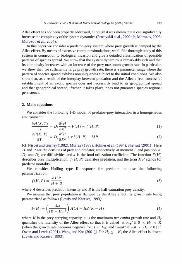
[cf. Nisbet and Gurney (1982), Murray (1989), Holmes et al. (1994), Sherratt (2001)]. HereH andP are the densities of prey and predator, respectively, at momentT and positionX .D1 and D2 are diffusivities andκ is the food utilization coefficient. The functionF(H )

describes prey multiplication,f (H, P) describes predation, and the termM P stands forpredator mortality.

We consider Holling type II response for predator and use the followingparametrization:

f (H, P) = AH P

H + B(3)

whereA describes predation intensity andB is the half-saturation prey density.We assume that prey population is damped by the Allee effect, its growth rate being

parametrized as follows (Lewis and Kareiva, 1993):

F(H ) =(

4ω

(K − H0)2

)H (H − H0)(K − H ) (4)

whereK is the prey carrying capacity,ω is the maximumper capita growth rate andH0quantifies the intensity of the Allee effect so that it is called ‘strong’ if 0< H0 < K(when the growth rate becomes negative forH < H0) and ‘weak’ if −K < H0 ≤ 0 [cf.Owen and Lewis (2001), Wang and Kot (2001)]. For H0 ≤ −K , the Allee effect is absent(Lewis and Kareiva, 1993).


For convenience, we introduce dimensionless variablesu = H/K , v = P/(κ K ),t = aT , x = X (a/D1)

1/2 wherea = Aκ K/B. Then, from Eqs. (1) and (2), we obtain:

∂u(x, t)

∂ t= ∂2u

∂x2 + γ u(u − β)(1 − u) − uv

1 + αu, (5)

∂v(x, t)

∂ t= ε

∂2v

∂x2+ uv

1 + αu− δv. (6)

Eqs. (5) and (6) contain five dimensionless parameters (against nine in the originalequations), i.e.,α = K/B, β = H0/K , γ = 4ωB K/(Aκ(K − H0)

2), δ = M/a andε = D2/D1. Thus, the behaviour of dimensionless solutionsu andv appears to dependon five dimensionless combinations of the original parameters rather than on each of themseparately.

Invasion of an alien species is usually started when a number of individuals of an exoticspecies is locally brought into the given ecosystem. From the point of model (5) and (6), itmeans that the initial species distribution should be described by functions of finite support.Thus, we consider initial conditions of the following form:

u(x, 0) = u0 for −∆u < x < ∆u, otherwise u(x, 0) = 0, (7)

v(x, 0) = v0 for −∆v < x < ∆v, otherwise v(x, 0) = 0 (8)

whereu0, v0 are the initial population densities and∆u , ∆v give the radius of the initiallyinvaded domain. Initial conditions (7) and (8) also correspond to the problem of biologicalcontrol when, soon enough after introduction of an exotic species, a predatory species isintroduced intentionally in an attempt to slow down or stop its spread [cf.Fagan and Bishop(2000), Owen and Lewis (2001), Petrovskii et al. (in press)].

Note that the initial conditions (7) and (8) aresomewhat idealized and in reality the formof the species initial distribution can be much more complicated. However, the results ofour computer simulations show that the type of the system dynamics depends more on theradius of the initially inhabited domain and onthe population density inside rather than onthe details of the population density profile.

3. Patterns of species spread

From the point of ecological applications, it is very important to distinguish betweenthe cases when invasion will likely be successful and the cases when it will likely fail.In practical ecology, invasion failure usually means that the introduced species fails toestablish itself in the new environment. Thus, an unsuccessful species is expected to goextinct soon after its introduction. However, it remains unclear whether invasion failuremay happen as well at later stages, i.e., whether invasive species can go extinct after havingalready spread over relatively large areas. Theresults that we present in this section showthat, for an invasive species affected by the Allee effect, extinction may take place at a laterstage after its geographical spread.

Moreover, it seems reasonable to distinguish between ‘geographical’ invasion and‘local’ invasion. We will call the invasion ‘local’ in the case when the new speciessuccessfully establishes itself locally, i.e., around the place of original introduction, but


does not spread over new areas due to the impact of certain factors. Correspondingly,we call the invasion ‘geographical’ in the case that the invasive species succeeds to spreadover largeareas. In many cases, local invasion of exotic species is followed by geographicalinvasion, although the time lag between these two stages can be as long as a few decades.The question that still needs to be answered is what environmental or biological factorsmake this lag so long and whether local invasion must always be followed, sooner or later,by geographical invasion. The results that wepresent below show that an exotic species caninvade locally but sometimes fails to invade geographically due to the interplay betweenpredation and the Allee effect.

Eqs. (5) and (6) with the initial conditions (7) and (8) were solved numerically in thedomain−L < x < L by finite-difference method. The steps of the numerical mesh werechosen asx = 0.2 andt = 0.001 and it was checked that a decrease of the mesh stepsdid not lead to any significant modification of the results. The ‘no-flux’ condition was usedat the boundaries and the radiusL of the numerical domain was chosen large enough inorder to make the impact of the boundaries as small as possible during the simulation time.Throughout this section we fixε = 1, the effect of differential diffusivity will be addressedin Section 5.

In order to identify different regimes and to reveal the corresponding structure of theparameter space, in total, over three thousand computer experiments were run for differentparameter values. We obtain that all regimes observed in our simulations can be classifiedinto three groups, seeFig. 1. These groups correspond to extinction, geographical invasionwhen the species keep spreading until they reach the domain boundaries, and regionalpersistence when the alien species invade locally and spread over a certain area but do notgo farther.

Before proceeding to regime description, the issue of regime dependence on the initialconditions should be clarified. It is well-known that in a predator–prey system with logisticgrowth for prey, although the population density can fall to very small values, the specieswill never go extinct in the strict mathematical sense because the extinction state (0, 0) isunstable (Gilpin, 1972) and thus acts as a ‘repeller’. Evolution of the initial conditions (7)and (8) eventually leads, for any biologically reasonable parameter values, to formation ofa travelling population front. Thus, the large-time asymptotical system dynamics does notdepend on the initial conditions as long asthey are described by finite functions (Volpertet al., 1994). Although the actual patterns of spread can be different for different parametervalues, e.g., front propagation can be followed either by a steady spatially homogeneousspecies distribution or by spatiotemporal pattern formation in the wake (Sherratt et al.,1995; Petrovskii et al., 1998; Petrovskii and Malchow, 2000), any introduction of a newspecies will lead to its geographical invasion. This prediction of inevitable species spreaddoes not seem realistic and was used as a justification for various modifications of themodel, e.g., by implementing a threshold at low population densities (Brauer and Soudack,1978; Wilson, 1998; Petrovskii and Shigesada, 2001).

The situation becomes different when the invasive prey is affected by the Allee effect.In this case, already single-species modelspredict that the introduced species does goextinct when the population size is not large enough (Lewis and Kareiva, 1993; Petrovskii,1994; Petrovskii and Shigesada, 2001). [Note that this phenomenon is often observed innature aswell, seeCourchamp et al. (1999).] The impact of predation makes this threshold


Fig. 1. Classification of invasion regimes.

behaviour more prominent, cf.Section 3.2. Essentially, for any value of parameters inEqs. (5) and (6), sufficiently smallu0 and/or∆u can turn any regime of species spread toextinction. In order to exclude this somewhat trivial case, in our computer experimentsu0and∆u are always chosen sufficiently large.

3.1. Regimes of geographical invasion

We begin with the regimes describing the unbounded spread of the invasive specieswhich corresponds to the geographical stage of biological invasion. We found threedifferent scenarios of the species spread, examples are shown inFigs. 2–8.

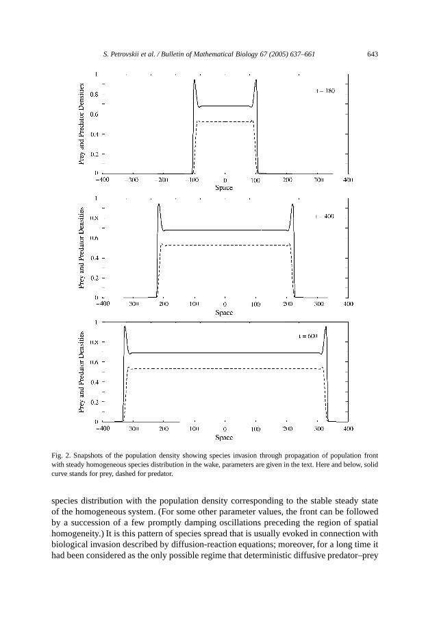
According to the first scenario, the species is spreading over space through propagationof a travelling population front, seeFigs. 2–5. In front of the front the species is absent,behind the front it is present in considerable densities. Apparently, this type of speciesspread corresponds to successful invasion. Depending on parameter values, in the wake ofthe front there can arise either a stationary spatially homogeneous species distribution orirregular spatiotemporal population oscillations.

Fig. 2shows the snapshots of the population density (solid curve stands for prey, dashedfor predator) obtained for parametersα = 0.5, β = 0.27, γ = 3, δ = 0.51. Hereand below (except forFig. 5), the initial conditions are∆u = 7, ∆v = 2, u0 = 1,v0 = 0.1. Propagation of the population front isfollowed by a stationary homogeneous


Fig. 2. Snapshots of the population density showing species invasion through propagation of population frontwith steady homogeneous species distribution in the wake, parameters are given in the text. Here and below, solidcurve standsfor prey, dashed for predator.

species distribution with the population density corresponding to the stable steady stateof the homogeneous system. (For some other parameter values, the front can be followedby a succession of a few promptly damping oscillations preceding the region of spatialhomogeneity.) It isthis pattern of species spread that is usually evoked in connection withbiological invasion described by diffusion-reaction equations; moreover, for a long time ithad been considered as the only possible regime that deterministic diffusive predator–prey


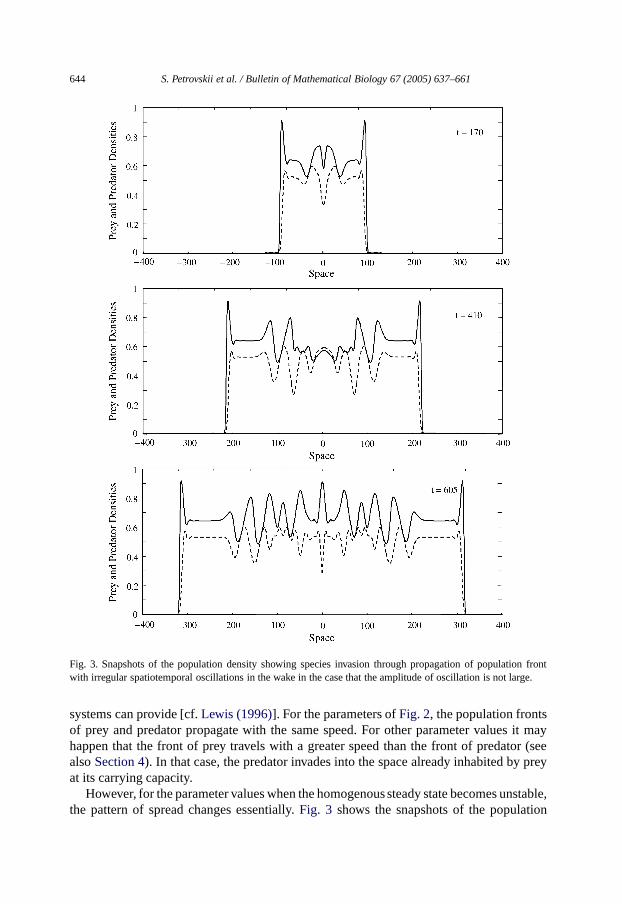
Fig. 3. Snapshots of the population density showing species invasion through propagation of population frontwith irregular spatiotemporal oscillations in the wake in the case that the amplitude of oscillation is not large.

systemscan provide [cf.Lewis (1996)]. For the parameters ofFig. 2, the population frontsof prey and predator propagate with the same speed. For other parameter values it mayhappen that the front of prey travels with a greater speed than the front of predator (seealsoSection 4). In that case, the predator invades into the space already inhabited by preyat its carrying capacity.

However, for the parameter values when the homogenous steady state becomes unstable,the pattern of spread changes essentially.Fig. 3 shows the snapshots of the population


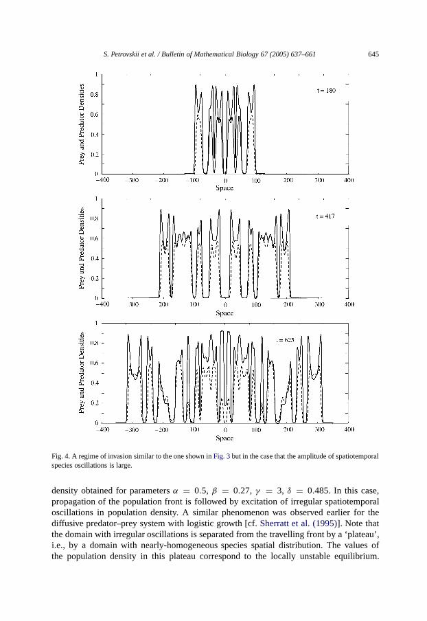
Fig. 4. A regime of invasion similar to the one shown inFig. 3but in thecase that the amplitude of spatiotemporalspecies oscillations is large.

density obtained for parametersα = 0.5, β = 0.27, γ = 3, δ = 0.485. In this case,propagation of the population front is followed by excitation of irregular spatiotemporaloscillations in population density. A similar phenomenon was observed earlier for thediffusive predator–prey system with logistic growth [cf.Sherratt et al. (1995)]. Note thatthe domain with irregular oscillations is separated from the travelling front by a ‘plateau’,i.e., by a domain with nearly-homogeneous species spatial distribution. The values ofthe population density in this plateau correspond to the locally unstable equilibrium.


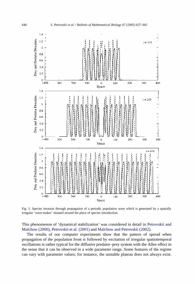
Fig. 5. Species invasion through propagation of a periodic population wave which is generated by a spatiallyirregular ‘wave-maker’ situated around the place of species introduction.

This phenomenon of ‘dynamical stabilization’ was considered in detail inPetrovskii andMalchow (2000), Petrovskii et al. (2001)andMalchow and Petrovskii (2002).

The results of our computer experiments show that the pattern of spread whenpropagation of the population front is followed by excitation of irregular spatiotemporaloscillations is rather typical for the diffusive predator–prey system with the Allee effect inthe sense that it can be observed in a wide parameter range. Some features of the regimecan vary with parameter values; for instance, the unstable plateau does not always exist.


Fig. 6. Snapshots of the population density (only half of the domain is shown) showing species spread over spacethrough propagation of a solitary moving population patch, or a ‘pulse’. Note that this pattern of spread does notlead to species invasion because thepopulation density in the wake is zero.

Also, for some parameters the amplitude of population oscillations becomes notably largerso that the pattern in the wake becomes more prominent, seeFig. 4obtained forα = 0.5,β = 0.27,γ = 3, δ = 0.47. Note that, although in this case the pattern as a whole lookslike an ensemble of separated patches, the scenario of species invasion is still essentiallythe same: close inspection of the population density snapshots clearly reveals the travellingpopulation front, cf. top, middle and bottom ofFig. 4.


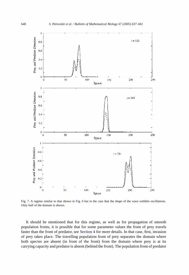
Fig. 7. A regime similar to that shown inFig. 6 but in the case that the shape of the wave exhibits oscillations.Only half of the domain is shown.

It should be mentioned that for this regime, as well as for propagation of smoothpopulation fronts, it is possible that for some parameter values the front of prey travelsfaster than the front of predator, seeSection 4for more details. In that case, first, invasionof prey takes place. The travelling population front of prey separates the domain whereboth species are absent (in front of the front) from the domain where prey is at itscarrying capacity and predator is absent (behind the front). The population front of predator


Fig. 8. A regime of invasion through propagation of separate patches and groups of patches.

propagates into the region already inhabited by prey, in the wake of the predator frontirregular population oscillations arise.

In the cases shown inFigs. 3and4, thepatches arising behind the front are irregular.For other parameter values, however, the spatial structure can be more regular.Fig. 5showsthe snapshots of the population density obtained for parametersα = 0.5,β = 0.28,γ = 7,δ = 0.46 and the initial conditions∆u = 5, ∆v = 3, u0 = 1, v0 = 1. In this case, speciesinvasion takes place through propagation of aperiodic travelling wave. The periodic waveis generated by an irregular ‘wave-maker’ situated about the place of the initial species


distribution, i.e., aroundx = 0. Depending on parameter values, the wave-maker eitherstays localized or gradually grows in size. In the latter case, the periodic oscillations areeventually displaced by irregular ones [cf.Petrovskii and Malchow (2001)for a similarphenomenon].

Al l the regimes described above correspond to species invasion through propagation ofa population front. According to the second scenario, the species spread over the domainvia propagation of a moving patch, or ‘pulse’, cf.Figs. 6and7 (only a half of the domain isshown). The dynamics is similar to predator–prey pursuit [cf.Murray (1989)]. In this case,the invasive species is absent both in frontof the pulse and in itswake which apparentlymeans that invasion fails in spite of the fact that geographical spread has taken place.Depending on parameter values, the travelling population pulse can be either stationarywhen its shape does not change with time, ornonstationary when its shape oscillates withtime; in both cases the pulse propagates with a constant speed.Fig. 6shows the snapshotsof the population density obtained for parametersα = 0.5, β = 0.28, γ = 3, δ = 0.44when the species spread over the system via propagation of a stationary travelling pulse.Fig. 7 is obtained forα = 0.5, β = 0.28, γ = 3, δ = 0.425, it shows propagation of anonstationary pulse.

Finally, there isanother, more exotic scenario of species geographical spread.Fig. 8shows the snapshots of the population density obtained for parametersα = 0.05,β = 0.28,γ = 3, δ = 0.52. In this case, invasion takes place through formation and propagation ofgroups of moving patches. However, the patch motion is now much more complicated thanthe simple locomotion in the case of travelling pulses. The patches interact with each other,they merge and split, some of the patches or even groups of patches can disappear, newpatches are formed, they can produce new groups of patches, etc. The inhabited area growsand eventually the groups of nonstationary patches occupy the whole domain. Althoughthere is certain visual similarity between this regime of invasion and the regime shownin Fig. 4, comparison between the snapshots obtained for different times immediatelyshows that in this case there is no stationary travelling population front. Another importantdistinction is that the size of the domain occupied by the moving patches does not growmonotonically, cf. top, middle and bottom ofFig. 8. That happens when the leading groupof patches goes extinct in the course of the system dynamics.

3.2. Regimes of anomalous extinction

The second group of regimes corresponds to species extinction. It is well-known that,in case the introduced species is affected by the Allee effect, it goes extinct if the initialpopulation size is not large enough, i.e., either the radius of originally inhabited domainor the population density inside are less than certain critical values (Lewis and Kareiva,1993; Petrovskii, 1994; Petrovskii and Shigesada, 2001). In this case, the population sizedecreases exponentially and the population stays localized in about the same domain whereit had originally been introduced. We will refer to this type of population dynamics as‘ordinary’ extinction.

When the introduced population is affected by predation, ‘ordinary’ extinction cantakes place as well. Although the critical values for theinitial radius and the initialprey density appear somewhat larger inthis case as a resultof the pressure from


the predator, the qualitative features of ‘ordinary’ extinction remain the same, cf.the previous paragraph. (Note that, in our model, extinction of prey inevitably leadsto extinction of both species.) However, due to the impact of predation, speciesextinction can also follow other, rather unusual scenarios. Depending on parametervalues, we observed two other regimes when species extinction is either preceded byformation of a distinct long-living spatiotemporal pattern or by long-distance populationspread.

Fig. 9shows the snapshots of the population density in the regime of species extinctionthrough ‘dynamical localization’ observed for parametersα = 0.1, β = 0.15, γ = 5,δ = 0.257. At an early stage of the system dynamics, a moving patch is formed whichpropagates with approximately constant speed over distances much longer compared to theradius of the initial species distribution. This stage of the system dynamics is apparentlysimilar to pulsepropagation, seeFig. 6. Finally, however, the prey is caught by the predatorand both species go extinct: starting from the moment shown in the bottom ofFig. 9 thepopulation size exhibits fast decay.

Fig. 10shows the regime of ‘patchy extinction’ (observed forα = 0.5,β = 0.2,γ = 1,δ = 0.365). In this case, the initial conditions eventually evolve into an ensemble of patchesallocated over the domain. The patches interact with each other in a complicated mannersomewhat similar to the patch dynamics shown inFig. 8; finally, however, the species goextinct.

Wewant to emphasize that, in both of these cases, the invasive population persists duringa remarkably long time before the actual population decay takes place (for the parametersof Figs. 9and 10, nearly one hundred times longer than it would be in the case of the‘ordinary’ extinction) and it can spread over large distances. During that period, the systemdynamics is very similar to the regimes of geographical spread shown inFigs. 6and8,respectively. These results seem to reveal a new aspect of the ‘extinction debt’ (Tilmanet al., 1994; Loehle and Li, 1996) and also evoke a more general discussion regarding theecological relevance of transient dynamics (Hastings, 2001): a population which is doomedto vanish, e.g., as a result ofcertain unfavourable environmental changes, can exhibit thedynamics which is, during a long time, virtually indistinguishable from the dynamics ofpersistent populations. The collapse comes unexpectedly and then it may be too late toapply a conservation strategy.

3.3. Regimes of local invasion

Remarkably, the two groups of the regimes described above, i.e., species extinction andunbounded spatial spread, do not exhaust all possible types of the system dynamics. Forcertain parameter values, evolution of the initial species distribution leads to formation ofquasistationary patches.Fig. 11 shows the snapshots obtained forα = 0.5, β = 0.32,γ = 3, δ = 0.455. In this case, at an early stage of the system dynamics (fort 100), twosymmetric dome-shaped patches are formed. At later stages, the position of their centresremains fixed and the shape of the patches changes with time in an oscillatory manner.A close inspection shows that, depending on the parameter values, the correspondingtemporal fluctuations in the population density can be either periodic or chaotic (Morozovet al., 2004).


Fig. 9. An example of ‘dynamical localization’: the population densities form a solitary moving patch whichpropagates a long distance before the speciesgo extinct. Only half of the domain is shown.

From the point of prospective ecological applications, this regime of the systemdynamics is probably the most interesting. Field observations give many examples whenthe invasive species, after introduction, remains localized inside a certain area during along time. Thus, their local invasion and subsequent regional persistence is not followedby geographical spread. There exist differentexplanations of this phenomenon such as theimpact of environmental borders, time-lag related tomutations and evolutionary changescaused by adaptation in the new environment, etc. Our results provide another explanation


Fig. 10. An example of long-living transients corresponding to the ‘patchy extinction’: species extinction ispreceded by spatiotemporal pattern formation going during a relatively long time.

and show that invasive species can be heldlocalized purely due to certain inter- andintraspecific interactions such as the interplay between the Allee effect and predation.

4. Parameter space structure

In the previous section, we demonstrated that the predator–prey system with the Alleeeffect for prey exhibits very rich dynamics and predicts a wide variety of patterns/regimes


Fig. 11. The regime of local invasion when the initial species introduction leads to formation of a few standingpatches. The position of the patches does not change with time while their shape is either stationary or oscillateswith time depending on parameter values.

of species spread. A natural question arising here is about the relation between theregimes and possible transition between themthat may take place in response to parametervariation. One way to address this issue is to study the structure of the system parameterspace in order to locate the domains corresponding to different regimes of invasion.

For that purpose, we fulfil a detailed numerical study of the system dynamics. In total,about three thousand computer experiments were run for different parameter values. The


Fig. 12. The map inthe parameter plane of the Eqs. (5) and (6) for γ = 1. Different domains correspond todifferent regimes, see details in the text.

results are shown inFigs. 12–14. Note that, since the model depends on four parameters(assuming here thatε = 1 is fixed,the caseε = 1 will be addressed separately in thenext section), it looks virtually impossible to accomplish a detailed study of the wholeR4+ parameter space. It is readily seen that in this case even as many as 104 computerexperiments, if run for parameter values spread homogeneously over the parameter space,would provide only meagre information about the position of different domains. In orderto overcome this difficulty, we apply a certain strategy in choosing parameter values. Sincethe main goal of this paper is to study the dynamics of invasive species subject to theinterplay between the impact of the Allee effect (quantified byβ) andpredation (quantifiedby δ), it looks more relevant to focus on the detailed structure of the(δ, β) plane.Correspondingly, we firstly choose a certain hypothetical value for the half-saturationdensity, i.e.,α = 0.5. Then we select a few values of the maximumper capita prey growthrate, i.e., in dimensionless units,γ = 1 (Fig. 12), γ = 3 (Fig. 13) andγ = 7 (Fig. 14).Then, for each of these values, the(δ, β) parameter plane was studied thoroughly.

In order to make the search in the(δ, β) plane more effective, one should also take intoaccount that nontrivial dynamics can only take place inside the rectangle0 < δ ≤ Ω =(1+α)−1, 0 < β ≤ 0.5. Hereδ is positive due to its biological meaning andβ is assumedto be positive because we are concerned with consequences of the strong Allee effect. Thevaluesδ > Ω = (1 + α)−1 correspond to predator extinction because the phase plane ofEqs. (5) and (6) in the spatially homogeneous case does not possess a co-existence steadystate in thebiologically meaningful domainu ≥ 0, v ≥ 0 and the ‘prey-only’ steady


Fig. 13. The map inthe parameter plane of the Eqs. (5) and (6) for γ = 3.

state (1, 0) is a stable node. The valuesβ > 0.5 are readily seen to always correspond tothe ‘ordinary extinction’ and thus are not of much interest either.

Fig. 12 shows themap in the (δ, β) plane obtained forγ = 1. Here domain 1corresponds to species extinction (including both ‘ordinary’ and ‘anomalous’ extinction).Domain 3 corresponds to geographical spread of invasive species either throughpropagation of population fronts with irregular spatiotemporal oscillation in the wake(Figs. 3and4) or through the spread of moving patches (Fig. 8). Since it is not alwayseasy to distinguish between these two regimes in numerical experiments, we are not goinginto the details of the ‘fine structure’ of domain 3. Domain 4 corresponds to geographicalinvasion through propagation of smooth population fronts with stationary homogeneousspecies distribution in the wake (Fig. 2). Sub-domain 4∗ corresponds to the case when thefront of invasive prey travels faster than the front of invasive predator, here the dashedcurve separating sub-domain 4∗ can be obtained analytically [cf.Petrovskii and Malchow(2000)]. Domain 5 corresponds to local invasion through formation of quasi-stationarypatches, seeFig. 11.

The structure of the(δ, β) parameter plane changes for larger values ofγ . Fig.13showsthe mapobtained forγ = 3, notations are the same as above. Now a new domain appears,i.e., domain 2 corresponding to propagation of solitary population pulses. Sub-domain 3∗corresponds to the case when the front of prey travels faster than the front of predator, cf.Section 3.1for details. A higher value ofγ corresponds to a ‘stronger’ prey; thus, it is notsurprising that the domain where the front of prey outruns the front of predator (below thedashed curve) has grown in size compared to the caseγ = 1 shown inFig. 12.


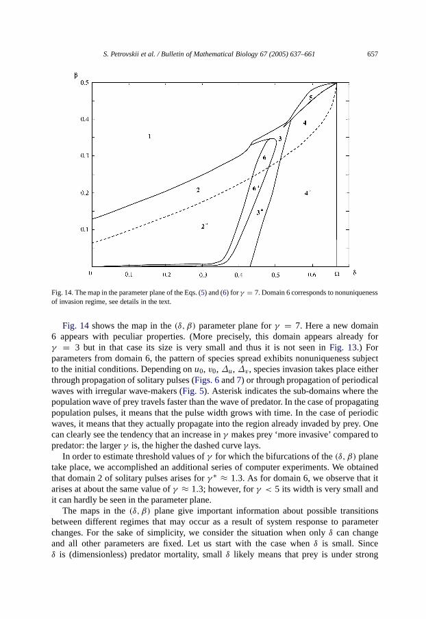
Fig. 14. The map inthe parameter plane of the Eqs. (5) and (6) for γ = 7. Domain 6 corresponds to nonuniquenessof invasion regime, see details in the text.

Fig. 14 shows themap in the(δ, β) parameter plane forγ = 7. Here a new domain6 appears with peculiar properties. (More precisely, this domain appears already forγ = 3 but in that case its size is very small and thus it is not seen inFig. 13.) Forparameters from domain 6, the pattern of species spread exhibits nonuniqueness subjectto the initial conditions. Depending onu0, v0, ∆u, ∆v, species invasion takes place eitherthrough propagation of solitary pulses (Figs. 6and7) or through propagation of periodicalwaves with irregular wave-makers (Fig. 5). Asterisk indicates the sub-domains where thepopulation wave of prey travels faster than the wave of predator. In the case of propagatingpopulation pulses, it means that the pulse width grows with time. In the case of periodicwaves, it means that they actually propagate into the region already invaded by prey. Onecan clearly see the tendency that an increase inγ makes prey ‘more invasive’ compared topredator: the largerγ is, thehigher the dashed curve lays.

In order to estimate threshold values ofγ for which the bifurcations of the(δ, β) planetake place, we accomplished an additional series of computer experiments. We obtainedthat domain 2 of solitary pulses arises forγ ∗ ≈ 1.3. As for domain 6, we observe that itarises at about the same value ofγ ≈ 1.3; however, forγ < 5 its width is very small andit can hardly be seen in the parameter plane.

The maps in the(δ, β) plane give important information about possible transitionsbetween different regimes that may occur as a result of system response to parameterchanges. For the sake of simplicity, we consider the situation when onlyδ can changeand all other parameters are fixed. Let us start with the case whenδ is small. Sinceδ is (dimensionless) predator mortality, smallδ likely means that prey is under strong


pressure from the predator. Thus, it is not surprising that smallδ typically correspondsto species extinction (unlessγ is sufficiently large andβ is sufficiently small, cf. theleft-hand bottom corner ofFig. 14). In order to avoid multivalence, we restrict furtheranalysis to the caseγ = 3. An increase inδ makes this pressure smaller and extinctionchanges, depending on other parameter values, either to local invasion (domain 5) or togeographical spread through pulse propagation (domain 2). Note that, since the impactof predation is still too strong, none of these two regimes lead to global persistenceof the invading species. However, further increase inδ changes these regimes first topatchy invasion (either preceded by population front propagation, cf.Figs. 3and4, or not,cf. Fig. 8) and then to invasion through propagation of smooth population fronts, seeFig. 2.Similar analysis can be made varying other parameters. In particular, it is straightforwardto see that similar succession of regimes takes place whenβ is varied from a large value toa smallone.

5. Concluding remarks

The impact of predation on the spread of invasive species has long been an issue ofsignificant interest (Murray, 1989; Sherratt et al., 1995; Shigesada and Kawasaki, 1997;Fagan and Bishop, 2000; Owen and Lewis, 2001; Petrovskii et al., in press). In mostcases, however, these studies were reduced to the case of populations with logistic growth.Meanwhile, for many ecological populations their growth rate is believed to be dampedby the Allee effect (Allee, 1938; Berryman, 1981). Although it was shown that the Alleeeffect can change population dynamics significantly (Dennis, 1989; Lewis and Kareiva,1993; Courchamp et al., 1999; Gyllenberg et al., 1999; Petrovskii et al., 2002a), its impacton species invasion has not been investigated in detail [but seeMorozov (2003)]. In thispaper we have shown, using a predator–prey system as a paradigm, that the spatiotemporaldynamics of invading species can become much more complex under the influence of theAllee effect and exhibit regimesof invasion that have not been studied theoretically before.A predator–prey system with the Allee effect for prey can exhibit such patterns of spreadas a patchy invasion (Fig. 8), geographical invasion without regional persistence (Figs. 6and 7) and local invasion without geographical spread (Fig. 11). Remarkably, similarpatterns are often observed in nature. In contrast, a predator–prey system without Alleeeffect only predicts species spread througheither smooth population waves or travellingfronts with population oscillations in the wake (similar to what is shown inFigs. 2, 3 and4respectively) [cf.Sherratt et al. (1995), Petrovskii et al. (1998), Petrovskii and Malchow(2000)].

By means of extensive numerical simulations, we revealed the structure of the parameterspace of the system. That structure gives important information about possible transitionsbetween different regimes of invasion. Here we consider one example how it can enhanceour understanding of various aspects of biological invasion. It is well-known that, betweenthe stage of exotic species establishment in the new environment and the stage of itsgeographical spread, there often exists a time-lag that can be sometimes as long as years,or even decades. The nature of this time-lag is widely seen in species adaptation to the newconditions. However, no specific dynamical mechanism has ever been proposed to explain


how species regional persistence actually changes to its geographical invasion. Our resultsseem to suggest such a mechanism. In an introduced species, the individual fitness undernew environmental conditionsis likely to be low which means that the species is moreprone to predation and to environmental stochasticity, so that the species is more likely togo extinct when it is at low density. Virtually, it means largeβ and/or smallδ. In terms ofthe diagrams shown inFigs. 12–14, it means that it falls either to domain 1 corresponding tospecies extinction or, in case fitness is not very low, to domain 5 corresponding to regionalpersistence. As a result of species adaptation to the new environment, the individual fitnessis likely to increase so that the parameters move from domain 5 either to domain 3or to domain 4; in both cases the regime of regional persistence gives way to speciesgeographical spread.

The results shown inFigs. 2–14wereobtained forε = D2/D1 = 1. However, we wantto emphasize that this not a principal limitation and the particular valueε = 1 was mainlychosen in order to exclude another parameter. Our tentative numerical simulations madefor 0.5 < ε < 2 show that all the regimes described above exist also in that case, althoughthe position of the domains in the(δ, β) plane is somewhat different.

The initial conditions that we used in numerical simulations correspond to the problemof biological control, see the lines after Eqs. (7) and (8). (Note that, in our computerexperiments, the radius of the domain initially inhabited by predator is always smallerthan that for prey.) Another biologically interesting case could be given by the situationwhen either prey is introduced into an ecosystem where predator is established, or predatoris introduced into an ecosystemwhere prey is established. Mathematically, it means thatonly one of the functionsu(x, 0) andv(x, 0) is finite. Although this problem still remainsto be investigated in detail, we fulfilled some tentative simulations to make an early insightinto the corresponding system dynamics. Our results indicate that, in this case, the numberof possible invasion regimes is likely to be less than it was for the problem (5)–(8);in particular we failed to observe the regimes shown inFigs. 6–11.

In this paper, our study of biological invasion has been restricted to the 1-D case. Thatwasdone mainly for practical reasons because thetime needed to fulfil necessary computersimulations increases essentially in the case of two spatial dimensions. However, we wantto mention that, although a regular investigation of this issue is still lacking, our tentativecomputer experiments indicate that the invasion patterns described above exist in the 2-Dpredator–prey system as well [cf. alsoPetrovskii et al. (2002a,b), Morozov (2003)].

In conclusion, we want to mention that the structure of the(δ, β) plane tends tobecome more complex with an increase inγ . This tendency can probably be easierunderstood if placed into a more general context of self-organization in dynamical systems.It is well-known from other branches of natural science that the dynamics of an opensystem becomes the more complicated the ‘more open’ it is, i.e., the higher is theenergy/mass input into a given system (Prigogine, 1980; Haken, 1983). In particular, ahigher energy/massinput drives the system further from its equilibrium state and enhancesformation of complex spatiotemporal patterns. [A classical example of this increasingcomplexity is given by the transition between laminar and turbulent flows in a pipewhich takes place when the speed of the fluid (and thus the mass/energy input) becomessufficiently high.] In the predator–prey model (1) and (2) the role of energy input that keepsthe system away from the trivial extinction equilibrium is played by the biomass increase


due to prey population growth. The prey growth is quantified by parameterγ ; thus, a highervalue ofγ makes the system ‘more open’ and increases its spatiotemporal complexity.

Acknowledgements

This work was partially supported by Russian Foundation for Basic Research undergrants 03-04-48018 and 04-04-49649, by U.S. National Science Foundation under grantsDEB-0080529 and DEB-0409984, by the University of California Agricultural ExperimentStation and by UCR Center for Conservation Biology.

References

Allee, W.C., 1938. The Social Life of Animals. Norton and Co, New York.Amarasekare, P., 1998. Interactions between local dynamics and dispersal: insights from single species models.

Theor. Popul. Biol. 53, 44–59.Berryman, A.A., 1981. Population Systems: A General Introduction. Plenum Press, New York.Brauer, F., Soudack, A.C., 1978. Response of predator–prey systems to nutrient enrichment and proportional

harvesting. Int. J. Control 27, 65–86.Courchamp, F., Clutton-Brock, T., Grenfell, B., 1999. Inverse density dependence and the Allee effect. TREE 14,

405–410.Dennis, B., 1989. Allee effects: population growth, critical density, and the chance of extinction. Nat. Res. Model.

3, 481–538.Fagan, W.F., Bishop, J.G., 2000. Trophic interactions during primary succession: herbivores slow a plant

reinvasion at Mount St. Helens. Am. Nat. 155, 238–251.Fagan, W.F., Lewis, M.A., Neubert, M.G., van den Driessche, P., 2002. Invasion theory and biological control.

Ecol. Lett. 5, 148–157.Fisher, R., 1937. The wave of advance of advantageous genes. Ann. Eugenics 7, 255–369.Frantzen, J., van den Bosch, F., 2000. Spread of organisms: can travelling and dispersive waves be distinguished?

Basic Appl. Ecol. 1, 83–91.Gilpin, M., 1972. Enriched predator–prey systems: theoretical stability. Science 177, 902–904.Gyllenberg, M., Hemminki, J., Tammaru, T., 1999. Allee effects can both conserve and create spatial

heterogeneity in population densities. Theor. Popul. Biol. 56, 231–242.Haken, H., 1983. Advanced Synergetics. Springer, Berlin.Hastings, A., 1996. Models of spatial spread: a synthesis. Biol. Conserv. 78, 143–148.Hastings, A., 2001. Transient dynamics and persistence of ecological systems. Ecol. Lett. 4, 215–220.Hengeveld, R., 1989. Dynamics of Biological Invasions. Chapman and Hall, London.Holmes, E.E., Lewis, M.A., Banks, J.E., Veit, R.R.,1994. Partial differential equations in ecology: spatial

interactions and population dynamics. Ecology 75, 17–29.Keitt, T.H., Lewis, M.A., Holt, R.D., 2001. Allee effects, invasion pinning, and species’ borders. Am. Nat. 157,

203–216.Lewis,M.A., 1996. A Tale of Two Tails: The Mathematical Links Between Dispersal, Patchiness and Variability

in Biological Invasion. Abstracts of the 3rd European Conference on Mathematics in Biology and Medicine,Heidelberg.

Lewis, M.A., Kareiva, P., 1993. Allee dynamics and the spread of invading organisms. Theor. Popul. Biol. 43,141–158.

Loehle, C., Li, B.-L., 1996. Habitat destruction and the extinction debt revisited. Ecol. Appl. 6, 784–789.Malchow, H., Petrovskii, S.V., 2002. Dynamical stabilization of an unstable equilibrium in chemical and

biological systems. Math. Comput. Model. 36, 307–319.Morozov, A.Y., 2003. Mathematical modelling of ecologicalfactors affecting stability and pattern formation in

marine plankton communities, Ph.D. Thesis, Shirshov Institute of Oceanology, Moscow, Russia.


Morozov, A.Y., Petrovskii, S.V., Li, B.-L., 2004. Bifurcations and chaos in a predator–prey system with the Alleeeffect. Proc. R. Soc. Lond. B 271, 1407–1414.

Murray, J.D., 1989. Mathematical Biology. Springer, Berlin.Nisbet, R.M., Gurney, W.S.C., 1982. Modelling Fluctuating Populations. Wiley, Chichester.Okubo, A., 1980. Diffusion and Ecological Problems:Mathematical Models. Springer, Berlin.Owen, M.R., Lewis, M.A., 2001. How predation can slow, stop or reverse a prey invasion. Bull. Math. Biol. 63,

655–684.Petrovskii, S.V., 1994. Approximate determination of themagnitude of the critical size in the problem of the

evolution of an impact. J. Eng. Phys. Thermophys. 66, 346–352.Petrovskii, S.V., Kawasaki, K., Takasu, F., Shigesada, N., 2001. Diffusive waves, dynamical stabilization and

spatio-temporal chaos in a community of three competitive species. Japan J. Indust. Appl. Math. 18, 459–481.Petrovskii, S.V., Malchow, H., 2000. Critical phenomena in plankton communities: KISS model revisited.

Nonlinear Analysis: Real World Applications 1, 37–51.Petrovskii, S.V., Malchow, H., 2001. Wave of chaos: new mechanism of pattern formation in spatio-temporal

population dynamics. Theor. Popul. Biol. 59, 157–174.Petrovskii, S.V., Malchow, H., Li, B.-L., 2004. An exact solution of a diffusive predator–prey system. Proc. R.

Soc. Lond. A (in press).Petrovskii, S.V., Shigesada, N., 2001. Some exact solutionsof a generalized Fisher equation related to the problem

of biological invasion. Math. Biosci. 172, 73–94.Petrovskii, S.V., Vinogradov, M.E., Morozov, A.Y.,1998. Spatial-temporal dynamics of a localized population

‘burst’ in a distributed prey–predator system. Oceanology 38, 796–804.Petrovskii, S.V., Morozov, A.Y., Venturino, E., 2002a. Allee effect makes possible patchy invasion in a

predator–prey system. Ecol. Lett. 5, 345–352.Petrovskii, S.V., Vinogradov, M.E., Morozov, A.Y., 2002b.Spatio-temporal horizontal plankton patterns caused

by biological invasion in a two-species model of plankton dynamics allowing for the Allee effect. Oceanology42, 384–393.

Prigogine, I., 1980. From Being to Becoming. Freeman and Co, San Francisco.Sakai, A.K. et al., 2001. The population biology ofinvasive species. Annu. Rev. Ecol. Syst. 32, 305–332.Sherratt, J.A., 2001. Periodic travelling waves in cyclic predator–prey systems. Ecol. Lett. 4, 30–37.Sherratt, J.A., Lewis, M.A., Fowler, A.C., 1995. Ecologicalchaos in the wake of invasion. Proc. Natl. Acad. Sci.

USA 92, 2524–2528.Shigesada, N., Kawasaki, K., 1997. Biological Invasions: Theory and Practice. Oxford University Press,

Oxford.Skellam, J.G., 1951. Random dispersal in theoretical populations. Biometrika 38, 196–218.Tilman, D., May, R.M., Lehman, C.L., Nowak, M.A., 1994. Habitat destruction and the extinction debt. Nature

371, 65–66.Volpert, A.I., Volpert, V.A., Volpert, V.A., 1994. Travelling Wave Solutions of Parabolic Systems. American

Mathematical Society, Providence.Wang, M.-E., Kot, M., 2001. Speeds of invasion in a model with strong or weak Allee effects. Math. Biosci. 171,

83–97.Wilson, W., 1998. Resolving discrepancies between deterministic population models and individual-based

simulations. Am. Nat. 151, 116–134.

Regimes of biological invasion in a predator–prey system ... · Main equations We c onsider the...

Documents

Transcript of Regimes of biological invasion in a predator–prey system ... · Main equations We c onsider the...