Reflection-Aware Sound Source Localization

Inkyu An1, Myungbae Son2, Dinesh Manocha3, and Sung-eui Yoon4

(http://sglab.kaist.ac.kr/RA-SSL)

Abstract— We present a novel, reflection-aware method for3D sound localization in indoor environments. Unlike priorapproaches, which are mainly based on continuous soundsignals from a stationary source, our formulation is designed tolocalize the position instantaneously from signals within a singleframe. We consider direct sound and indirect sound signalsthat reach the microphones after reflecting off surfaces suchas ceilings or walls. We then generate and trace direct andreflected acoustic paths using inverse acoustic ray tracing andutilize these paths with Monte Carlo localization to estimate a3D sound source position. We have implemented our methodon a robot with a cube-shaped microphone array and testedit against different settings with continuous and intermittentsound signals with a stationary or a mobile source. Acrossdifferent settings, our approach can localize the sound with anaverage distance error of 0.8 m tested in a room of 7 m by 7 marea with 3 m height, including a mobile and non-line-of-sightsound source. We also reveal that the modeling of indirect raysincreases the localization accuracy by 40% compared to onlyusing direct acoustic rays.

I. INTRODUCTION

Robots are increasingly used in our daily environments,and the demands on robots to interact with humans andthe environment using acoustic cues are getting stronger.The recent popularity of intelligent devices such as AmazonEcho and Google Home is giving rise to new challengesin acoustic scene analysis. One of the key issues in theseapplications is localizing the exact position of a sound sourcein the real world. Once a robot identifies the location of thesound source, it can approach the location and perform manyuseful tasks. The resulting problem, sound source localiza-tion (SSL), has been well-formulated and well-studied fordecades [1].

Most prior work in SSL has been related to the design ofmicrophone arrays and the use of digital signal processingtechniques. Nonetheless, it remains a challenging problemto exactly locate the sound source with limited informationavailable from the sensors equipped on a robot. In the mostgeneral setting, the localization problem tends to be ill-posed. Most of the research in the last two decades hasbeen dedicated to capturing the local characteristics of inputsignals, such as incoming directions of a sound. Specifically,Time Difference of Arrival (TDOA) based SSL techniqueshave been investigated for the last two decades, and mainlyutilize the difference of arrival time between two microphone

1Inkyu An, 2Myungbae Son, and 4Sung-eui Yoon (Corresponding author)are with the School of Computing, KAIST, Daejeon, South Korea; 3DineshManocha is with the Department of Computer Science, UNC-ChapelHill, USA; {inkyu.an, nedsociety}@kaist.ac.kr,dm@cs.unc.edu, sungeui@kaist.edu

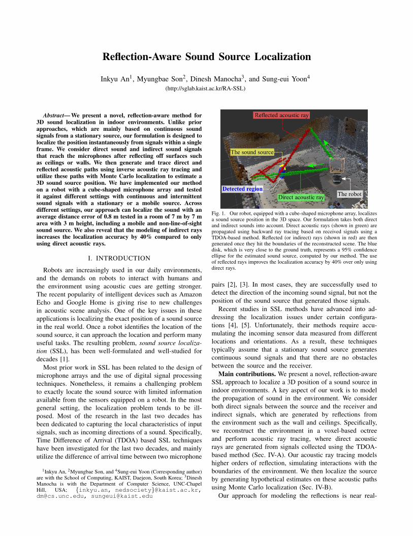
Fig. 1. Our robot, equipped with a cube-shaped microphone array, localizesa sound source position in the 3D space. Our formulation takes both directand indirect sounds into account. Direct acoustic rays (shown in green) arepropagated using backward ray tracing based on received signals using aTDOA-based method. Reflected (or indirect) rays (shown in red) are thengenerated once they hit the boundaries of the reconstructed scene. The bluedisk, which is very close to the ground truth, represents a 95% confidenceellipse for the estimated sound source, computed by our method. The useof reflected rays improves the localization accuracy by 40% over only usingdirect rays.

pairs [2], [3]. In most cases, they are successfully used todetect the direction of the incoming sound signal, but not theposition of the sound source that generated those signals.

Recent studies in SSL methods have advanced into ad-dressing the localization issues under certain configura-tions [4], [5]. Unfortunately, their methods require accu-mulating the incoming sensor data measured from differentlocations and orientations. As a result, these techniquestypically assume that a stationary sound source generatescontinuous sound signals and that there are no obstaclesbetween the source and the receiver.

Main contributions. We present a novel, reflection-awareSSL approach to localize a 3D position of a sound source inindoor environments. A key aspect of our work is to modelthe propagation of sound in the environment. We considerboth direct signals between the source and the receiver andindirect signals, which are generated by reflections fromthe environment such as the wall and ceilings. Specifically,we reconstruct the environment in a voxel-based octreeand perform acoustic ray tracing, where direct acousticrays are generated from signals collected using the TDOA-based method (Sec. IV-A). Our acoustic ray tracing modelshigher orders of reflection, simulating interactions with theboundaries of the environment. We then localize the sourceby generating hypothetical estimates on these acoustic pathsusing Monte Carlo localization (Sec. IV-B).

Our approach for modeling the reflections is near real-

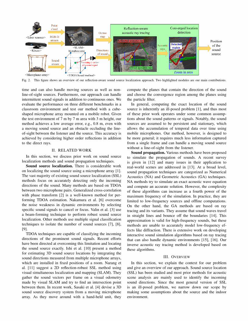
Fig. 2. This figure shows an overview of our reflection-aware sound source localization approach. Two highlighted modules are our main contributions.

time and can also handle moving sources as well as non-line-of-sight sources. Furthermore, our approach can handleintermittent sound signals in addition to continuous ones. Weevaluate the performance on three different benchmarks in aclassroom environment and test our method with a cube-shaped microphone array mounted on a mobile robot. Giventhe test environment of 7 m by 7 m area with 3 m height, ourmethod achieves a low average error, e.g., 0.8 m, even witha moving sound source and an obstacle occluding the line-of-sight between the listener and the source. This accuracy isachieved by considering higher order reflections in additionto the direct rays.

II. RELATED WORKIn this section, we discuss prior work on sound source

localization methods and sound propagation techniques.Sound source localization. There is considerable work

on localizing the sound source using a microphone array [1].The vast majority of existing sound source localization (SSL)methods focus on accurately detecting only the incomingdirections of the sound. Many methods are based on TDOAbetween two microphone pairs. Generalized cross-correlationwith phase transform [2] is a well-known method for per-forming TDOA estimation. Nakamura et al. [6] overcomethe noise weakness in dynamic environments by selectingspecific sound signals to cancel or focus. Valin et al. [3] usea beam-forming technique to perform robust sound sourcelocalization. Other methods use multiple signal classificationtechniques to isolate the number of sound sources [7], [8],[9].

TDOA techniques are capable of classifying the incomingdirections of the prominent sound signals. Recent effortshave been directed at overcoming this limitation and locatingthe sound source exactly. Ishi et al. [10] present a methodfor estimating 3D sound source locations by integrating thesound directions measured from multiple microphone arrays,which are installed in fixed positions of a room. Narang etal. [11] suggest a 2D reflection-robust SSL method usingvisual simultaneous localization and mapping (SLAM). Theygather the sound vectors per frame on a visual odometrymade by visual SLAM and try to find an intersection pointbetween them. In recent work, Sasaki et al. [4] devise a 3Dsound source discovery system from a moving microphonearray. As they move around with a hand-held unit, they

compute the planes that contain the direction of the soundand choose the convergence region among the planes usingthe particle filter.

In general, computing the exact location of the soundsource is inherently an ill-posed problem [1], and thus mostof these prior work operates under some common assump-tions about the sound patterns or signals. Notably, the soundsources are assumed to be persistent and stationary, whichallows the accumulation of temporal data over time usingmobile microphones. Our method, however, is designed tobe more general; it requires much less information capturedfrom a single frame and can handle a moving sound sourcewithout a line-of-sight from the listener.

Sound propagation. Various methods have been proposedto simulate the propagation of sounds. A recent surveyis given in [12] and many issues in their application toreal-world scenes are addressed in [13]. At a broad level,sound propagation techniques are categorized as NumericalAcoustics (NA) and Geometric Acoustics (GA) techniques.NA methods try to simulate an exact acoustic wave equationand compute an accurate solution. However, the complexityof these algorithms can increase as a fourth power of themaximum frequency of the simulation. In practice, they arelimited to low-frequency sources and offline computations.On the other hand, the GA methods are based on raytracing and its variants. They assume that sound waves travelin straight lines and bounce off the boundaries [14]. Thisapproximation is valid for high-frequency sounds, but thesemethods are unable to accurately model low-frequency ef-fects like diffraction. There is extensive work on developinginteractive sound simulation algorithms based on ray tracingthat can also handle dynamic environments [15], [16]. Ourinverse acoustic ray tracing method is developed based onthese algorithms.

III. OVERVIEW

In this section, we explain the context for our problemand give an overview of our approach. Sound source location(SSL) has been studied and most prior methods for acousticscene analysis are mainly used to identify the incomingsound directions. Since the most general version of SSLis an ill-posed problem, we narrow down our scope bymaking some assumptions about the source and the indoorenvironment.

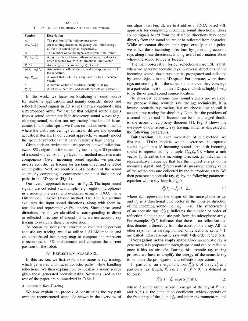
TABLE ITHIS TABLE LISTS COMMONLY APPEARING NOTATIONS.

Symbol Descriptionom The position of the microphone array.(vn, fn, ikn) An incoming direction, frequency and initial energy

of the n-th sound signal, respectively.N The number of sound signals at current time frame.Rn, rk

n, dn A ray path traced from n-th sound signal, and its k-thorder reflected ray with its directional unit vector.

Ikn(l′) An energy of the sound ray rk

n at l = l′.α( fn),αs( fn) Attenuation coeff. of the air, and absorption coeff. of

the reflection.phit ,Plocal A voxel that is hit by a ray, and its local, occupied

voxels.n A normal vector of a surface locally fit at phit .χt ,xi

t A set of W particles, and its i-th particle at iteration t.

In this work, we focus on localizing a sound sourcefor real-time applications and mainly consider direct andreflected sound signals in 3D scenes that are captured usinga microphone array. We assume that original sound signalsfrom a sound source are high-frequency sound waves (e.g.,clapping sound) so that our ray tracing based model is ac-curate. In a similar spirit, we focus on indoor environments,where the walls and ceilings consist of diffuse and specularacoustic materials. In our current approach, we mainly modelthe specular reflections that carry relatively high energy.

Given such an environment, we present a novel reflection-aware SSL algorithm for accurately localizing a 3D positionof a sound source. At a high level, our method uses two maincomponents. Given incoming sound signals, we performinverse acoustic ray tracing for tracking direct and reflectedsound paths. Next, we identify a 3D location of the soundsource by computing a convergence point of those tracedpaths in the 3D space (Fig. 1).

Our overall approach is shown in Fig. 2. The input soundsignals are collected via multiple (e.g., eight) microphonesin a microphone array and evaluated using a TDOA (TimeDifference Of Arrival) based method. The TDOA algorithmevaluates the input sound directions, along with their in-tensities and representative frequencies. Since these sounddirections are not yet classified as corresponding to director reflected directions of sound paths, we use acoustic raytracing to evaluate their characteristics.

To obtain the necessary information required to performacoustic ray tracing, we also utilize a SLAM module andan octree-based occupancy map to compute and representa reconstructed 3D environment and compute the currentposition of the robot.

IV. REFLECTION-AWARE SSLIn this section, we first explain our acoustic ray tracing,

which generates and traces acoustic paths, while handlingreflections. We then explain how to localize a sound sourcegiven those generated acoustic paths. Notations used in therest of the paper are summarized in Table I.

A. Acoustic Ray TracingWe now explain the process of constructing the ray path

over the reconstructed scene. As shown in the overview of

our algorithm (Fig. 2), we first utilize a TDOA based SSLapproach for computing incoming sound directions. Thesesound signals heard from the detected directions may comedirectly from the sound source or be reflected from obstacles.While we cannot discern their types exactly at this point,we utilize these incoming directions by generating acousticrays along these directions, finding useful information aboutwhere the sound source is located.

The main observation for our reflection-aware SSL is that,when we generate acoustic rays in reverse directions of theincoming sound, those rays can be propagated and reflectedby some objects in the 3D space. Furthermore, when thoserays are coming from the same sound source, they convergein a particular location in the 3D space, which is highly likelyto be the original sound source location.

To inversely determine how sound signals are received,we propose using acoustic ray tracing; technically, it isinverse acoustic ray tracing, but we choose just to call itacoustic ray tracing for simplicity. Note that the positions ofa sound source and its listener can be interchanged thanksto the acoustic reciprocity theorem [1]. Fig. 3 shows theoverview of our acoustic ray tracing, which is discussed inthe following paragraphs.

Initialization. On each invocation of our method, wefirst run a TDOA module, which discretizes the capturedsound signal into N incoming sounds. An n-th incomingsound is represented by a tuple (vn, fn, i0n), where a unitvector vn describes the incoming direction, fn indicates therepresentative frequency that has the highest energy of theincoming signal, and i0n represents its measured energy valueof the sound pressure collected by the microphone array. Wethen generate an acoustic ray, r0

n, by the following parametricequation with a ray length, l ≥ 0:

r0n(l) = d0

n · l + om, (1)

where om represents the origin of the microphone array,and d0

n is a directional unit vector in the inverted directionof the incoming sound, i.e., d0

n = −vn. The superscript kof an acoustic ray, rk

n(l), indicates the number or order ofreflection along an acoustic path from the microphone array.For example, r0

n(l) indicates that there is no reflection andthus denotes a direct ray from the microphone array. All theother rays with a varying number of reflections, i.e. k ≥ 1,are called indirect acoustic rays with k-th order reflections.

Propagation in the empty space. Once an acoustic ray isgenerated, it is propagated through space and can be reflectedonce it hits an obstacle. During this acoustic ray tracingprocess, we have to amplify the energy of the acoustic rayto simulate the propagation and reflection operations.

In particular, an energy function, Ikn(l′), of a ray rk

n at aparticular ray length, l′, i.e. l = l′ (l′ ≥ 0), is defined asfollows:

Ikn(l′) = ikn · exp(α( fn)l′), (2)

where ikn is the initial acoustic energy of the ray at l′ = 0,and α( fn) is the attenuation coefficient, which depends onthe frequency of the sound fn, and other environment-related

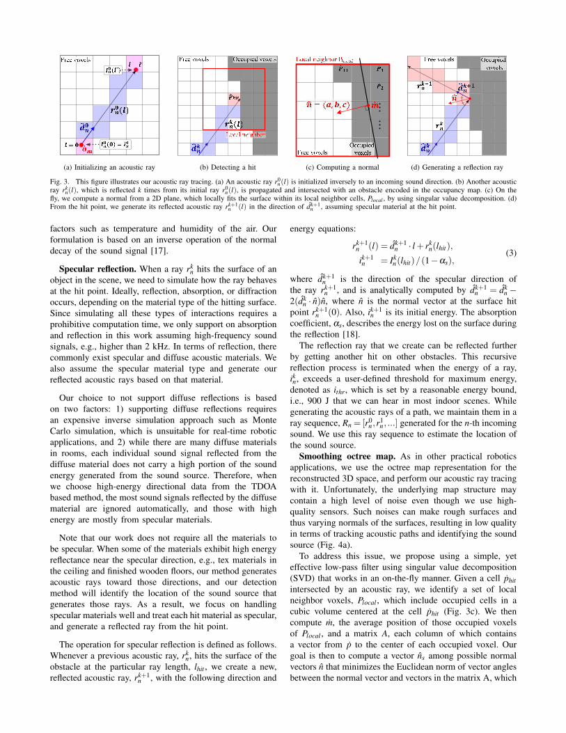
(a) Initializing an acoustic ray (b) Detecting a hit (c) Computing a normal (d) Generating a reflection ray

Fig. 3. This figure illustrates our acoustic ray tracing. (a) An acoustic ray r0n(l) is initialized inversely to an incoming sound direction. (b) Another acoustic

ray rkn(l), which is reflected k times from its initial ray r0

n(l), is propagated and intersected with an obstacle encoded in the occupancy map. (c) On thefly, we compute a normal from a 2D plane, which locally fits the surface within its local neighbor cells, Plocal , by using singular value decomposition. (d)From the hit point, we generate its reflected acoustic ray rk+1

n (l) in the direction of dk+1n , assuming specular material at the hit point.

factors such as temperature and humidity of the air. Ourformulation is based on an inverse operation of the normaldecay of the sound signal [17].

Specular reflection. When a ray rkn hits the surface of an

object in the scene, we need to simulate how the ray behavesat the hit point. Ideally, reflection, absorption, or diffractionoccurs, depending on the material type of the hitting surface.Since simulating all these types of interactions requires aprohibitive computation time, we only support on absorptionand reflection in this work assuming high-frequency soundsignals, e.g., higher than 2 kHz. In terms of reflection, therecommonly exist specular and diffuse acoustic materials. Wealso assume the specular material type and generate ourreflected acoustic rays based on that material.

Our choice to not support diffuse reflections is basedon two factors: 1) supporting diffuse reflections requiresan expensive inverse simulation approach such as MonteCarlo simulation, which is unsuitable for real-time roboticapplications, and 2) while there are many diffuse materialsin rooms, each individual sound signal reflected from thediffuse material does not carry a high portion of the soundenergy generated from the sound source. Therefore, whenwe choose high-energy directional data from the TDOAbased method, the most sound signals reflected by the diffusematerial are ignored automatically, and those with highenergy are mostly from specular materials.

Note that our work does not require all the materials tobe specular. When some of the materials exhibit high energyreflectance near the specular direction, e.g., tex materials inthe ceiling and finished wooden floors, our method generatesacoustic rays toward those directions, and our detectionmethod will identify the location of the sound source thatgenerates those rays. As a result, we focus on handlingspecular materials well and treat each hit material as specular,and generate a reflected ray from the hit point.

The operation for specular reflection is defined as follows.Whenever a previous acoustic ray, rk

n, hits the surface of theobstacle at the particular ray length, lhit , we create a new,reflected acoustic ray, rk+1

n , with the following direction and

energy equations:

rk+1n (l) = dk+1

n · l + rkn(lhit),

ik+1n = Ik

n(lhit)/(1−αs),(3)

where dk+1n is the direction of the specular direction of

the ray rk+1n , and is analytically computed by dk+1

n = dkn −

2(dkn · n)n, where n is the normal vector at the surface hit

point rk+1n (0). Also, ik+1

n is its initial energy. The absorptioncoefficient, αs, describes the energy lost on the surface duringthe reflection [18].

The reflection ray that we create can be reflected furtherby getting another hit on other obstacles. This recursivereflection process is terminated when the energy of a ray,ikn, exceeds a user-defined threshold for maximum energy,denoted as ithr, which is set by a reasonable energy bound,i.e., 900 J that we can hear in most indoor scenes. Whilegenerating the acoustic rays of a path, we maintain them in aray sequence, Rn = [r0

n,r1n, ...] generated for the n-th incoming

sound. We use this ray sequence to estimate the location ofthe sound source.

Smoothing octree map. As in other practical roboticsapplications, we use the octree map representation for thereconstructed 3D space, and perform our acoustic ray tracingwith it. Unfortunately, the underlying map structure maycontain a high level of noise even though we use high-quality sensors. Such noises can make rough surfaces andthus varying normals of the surfaces, resulting in low qualityin terms of tracking acoustic paths and identifying the soundsource (Fig. 4a).

To address this issue, we propose using a simple, yeteffective low-pass filter using singular value decomposition(SVD) that works in an on-the-fly manner. Given a cell phitintersected by an acoustic ray, we identify a set of localneighbor voxels, Plocal , which include occupied cells in acubic volume centered at the cell phit (Fig. 3c). We thencompute m, the average position of those occupied voxelsof Plocal , and a matrix A, each column of which containsa vector from p to the center of each occupied voxel. Ourgoal is then to compute a vector ns among possible normalvectors n that minimizes the Euclidean norm of vector anglesbetween the normal vector and vectors in the matrix A, which

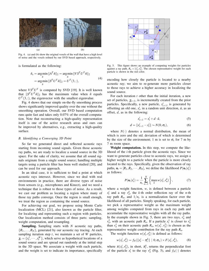
(a) (b)

Fig. 4. (a) and (b) show the original voxels of the wall that have a high levelof noise and the voxels refined by our SVD based approach, respectively.

is formulated as the following:

ns = argminn‖AT n‖2 = argmin

n‖V STUT n‖2

= argminn‖STUT n‖2 =UT (3, :),

(4)

where V STUT is computed by SVD [19]. It is well knownthat ‖STUT n‖2 has the maximum value when n equalsUT (3, :), the eigenvector with the smallest eigenvalue.

Fig. 4 shows that our simple on-the-fly smoothing processshows significantly improved quality over the one without thesmoothing operation. Overall, our SVD based computationruns quite fast and takes only 0.07% of the overall computa-tion. Note that reconstructing a high-quality representationitself is one of the active research areas and ours canbe improved by alternatives, e.g., extracting a high-qualitysurface.

B. Identifying a Converging 3D Point

So far we generated direct and reflected acoustic raysstarting from incoming sound signals. Given those acousticray paths, we are ready to localize a sound source in the 3Dspace. For the sake of clarity, we assume that all sound sig-nals originate from a single sound source; handling multipletargets using a particle filter has been well studied [20], andcan be used for our approach.

In an ideal case, it is sufficient to find a point at whichacoustic rays intersect. However, since we deal with realenvironments in practice, there are diverse types of noisefrom sensors (e.g., microphones and Kinect), and we need atechnique that is robust to those types of noise. As a result,we cast our problem as locating a region where many ofthose ray paths converge. Once the region is small enough,we treat the region as containing the sound source.

For achieving our goal, we propose using Monte Carlolocalization (MCL) [21], also known as the particle filter,for localizing and representing such a region with particles.Our localization method consists of three parts: sampling,weight computation, and resampling.

Sampling. Sampling starts with N acoustic ray paths,{R1, . . . ,RN}, generated by our acoustic ray tracing. At eachsampling iteration step t, we maintain a set of W particles,χt = {x1

t , · · · ,xWt }, which serve as hypothetical locations of a

sound source and are spread out randomly at the initial stepin the 3D space. We associate a weight with each particle,and the weight is set to indicate its importance, specifically

Fig. 5. This figure shows an example of computing weights for particlesagainst a ray path, Rn = [r1

n ,r2n ]. The chosen representative weight for each

particle is shown in the red color.

encoding how closely the particle is located to a nearbyacoustic ray; we aim to re-generate more particles closerto those rays to achieve a higher accuracy in localizing thesound source.

For each iteration t other than the initial iteration, a newset of particles, χt+1, is incrementally created from the priorparticles. Specifically, a new particle, xi

t+1, is generated byoffsetting an old one, xi

t , in a random unit direction, u, as anoffset, d, as in the following:

xit+1 = xi

t +d · u, (5)

d = ‖xit+1− xi

t‖∼ N(0,σs), (6)

where N(·) denotes a normal distribution, the mean ofwhich is zero and the std. deviation of which is determinedby the size of the environment; 1 m is set to σs for 7 m by7 m room space.

Weight computation. In this step, we compute the like-lihood of the i-th particle given the acoustic rays. Since wewant to generate particles close to acoustic rays, we assign ahigher weight to a particle when the particle is more closelylocated to the rays. Specifically, given the observation of raypaths, ot = [R1,R2, · · · ,RN ], we define the likelihood P(ot |xi

t)as follows:

P(ot |xit) =

1nc

N

∑n=1

{max

kw(xi

t ,rkn)

}, (7)

where a weight function, w, is defined between a particlexi

t and a ray rkn, the k-th order reflection ray of the n-th

ray path Rn, and 1/nc is a normalization factor over thelikelihood of all particles. Simply speaking, for each particle,we pick a representative weight as the maximum weightamong weights computed from rays in each ray path andaccumulate the representative weights with all the ray paths.In the example shown in Fig. 5, there are two rays, r1

n andr2

n, with an acoustic path Rn. If a particle x1t is closer to r2

nthan r1

n on their acoustic path Rn, w(x1t , r2

n) is chosen as therepresentative weight contribution for the ray path Rn.

The weight function w(xit ,r

kn) is defined as follows:

w(xit ,r

kn) = fN(‖xi

t −πki ‖ | 0,σw)×F(xi

t ,rkn), (8)

where π(xit ,r

kn), in short, πk

i , returns the perpendicular footof the particle xi

t to the ray rkn (Fig. 5), and fN(·) denotes

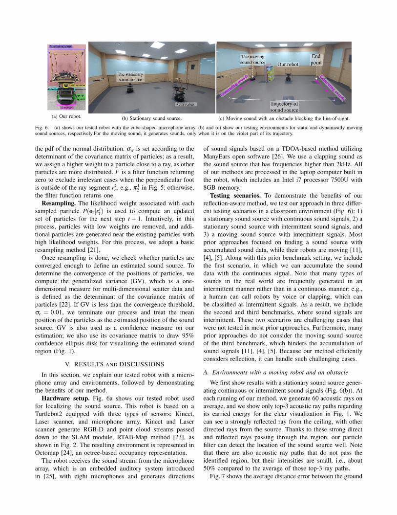
(a) Our robot. (b) Stationary sound source. (c) Moving sound with an obstacle blocking the line-of-sight.

Fig. 6. (a) shows our tested robot with the cube-shaped microphone array. (b) and (c) show our testing environments for static and dynamically movingsound sources, respectively.For the moving sound, it generates sounds, only when it is on the violet part of its trajectory.

the pdf of the normal distribution. σw is set according to thedeterminant of the covariance matrix of particles; as a result,we assign a higher weight to a particle close to a ray, as otherparticles are more distributed. F is a filter function returningzero to exclude irrelevant cases when the perpendicular footis outside of the ray segment rk

n, e.g., π12 in Fig. 5; otherwise,

the filter function returns one.Resampling. The likelihood weight associated with each

sampled particle P(ot |xit) is used to compute an updated

set of particles for the next step t + 1. Intuitively, in thisprocess, particles with low weights are removed, and addi-tional particles are generated near the existing particles withhigh likelihood weights. For this process, we adopt a basicresampling method [21].

Once resampling is done, we check whether particles areconverged enough to define an estimated sound source. Todetermine the convergence of the positions of particles, wecompute the generalized variance (GV), which is a one-dimensional measure for multi-dimensional scatter data andis defined as the determinant of the covariance matrix ofparticles [22]. If GV is less than the convergence threshold,σc = 0.01, we terminate our process and treat the meanposition of the particles as the estimated position of the soundsource. GV is also used as a confidence measure on ourestimation; we also use its covariance matrix to draw 95%confidence ellipsis disk for visualizing the estimated soundregion (Fig. 1).

V. RESULTS AND DISCUSSIONS

In this section, we explain our tested robot with a micro-phone array and environments, followed by demonstratingthe benefits of our method.

Hardware setup. Fig. 6a shows our tested robot usedfor localizing the sound source. This robot is based on aTurtlebot2 equipped with three types of sensors: Kinect,Laser scanner, and microphone array. Kinect and Laserscanner generate RGB-D and point cloud streams passeddown to the SLAM module, RTAB-Map method [23], asshown in Fig. 2. The resulting environment is represented inOctomap [24], an octree-based occupancy representation.

The robot receives the sound stream from the microphonearray, which is an embedded auditory system introducedin [25], with eight microphones and generates directions

of sound signals based on a TDOA-based method utilizingManyEars open software [26]. We use a clapping sound asthe sound source that has frequencies higher than 2kHz. Allof our methods are processed in the laptop computer built inthe robot, which includes an Intel i7 processor 7500U with8GB memory.

Testing scenarios. To demonstrate the benefits of ourreflection-aware method, we test our approach in three differ-ent testing scenarios in a classroom environment (Fig. 6): 1)a stationary sound source with continuous sound signals, 2) astationary sound source with intermittent sound signals, and3) a moving sound source with intermittent signals. Mostprior approaches focused on finding a sound source withaccumulated sound data, while their robots are moving [11],[4], [5]. Along with this prior benchmark setting, we includethe first scenario, in which we can accumulate the sounddata with the continuous signal. Note that many types ofsounds in the real world are frequently generated in anintermittent manner rather than in a continuous manner; e.g.,a human can call robots by voice or clapping, which canbe classified as intermittent signals. As a result, we includethe second and third benchmarks, where sound signals areintermittent. These two scenarios are challenging cases thatwere not tested in most prior approaches. Furthermore, manyprior approaches do not consider the moving sound sourceof the third benchmark, which hinders the accumulation ofsound signals [11], [4], [5]. Because our method efficientlyconsiders reflection, it can handle such challenging cases.

A. Environments with a moving robot and an obstacle

We first show results with a stationary sound source gener-ating continuous or intermittent sound signals (Fig. 6(b)). Ateach running of our method, we generate 60 acoustic rays onaverage, and we show only top-3 acoustic ray paths regardingits carried energy for the clear visualization in Fig. 1. Wecan see a strongly reflected ray from the ceiling, with otherdirected rays from the source. Thanks to these strong directand reflected rays passing through the region, our particlefilter can detect the location of the sound source well. Notethat there are also acoustic ray paths that do not pass theidentified region, but their intensities are small, i.e., about50% compared to the average of those top-3 ray paths.

Fig. 7 shows the average distance error between the ground

(a) Continuous sound

(b) Intermittent sound

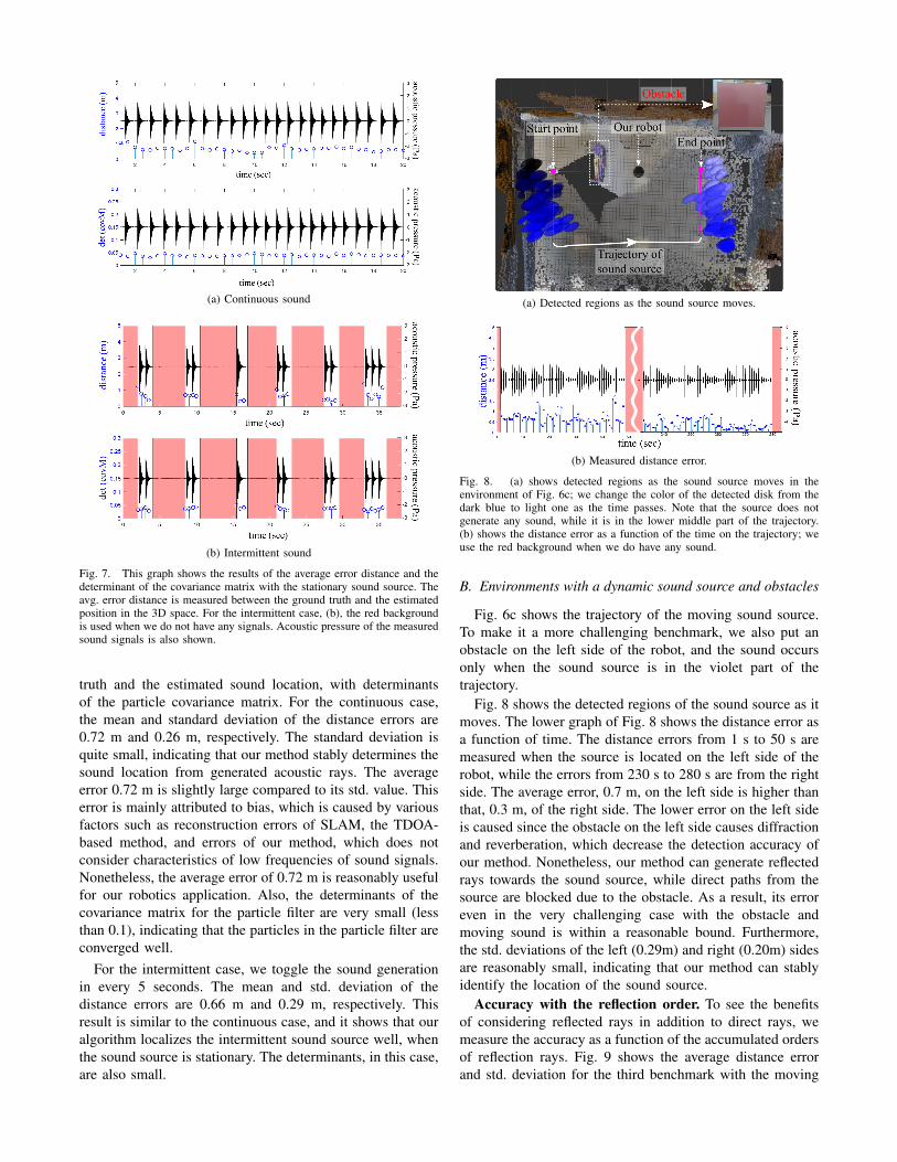
Fig. 7. This graph shows the results of the average error distance and thedeterminant of the covariance matrix with the stationary sound source. Theavg. error distance is measured between the ground truth and the estimatedposition in the 3D space. For the intermittent case, (b), the red backgroundis used when we do not have any signals. Acoustic pressure of the measuredsound signals is also shown.

truth and the estimated sound location, with determinantsof the particle covariance matrix. For the continuous case,the mean and standard deviation of the distance errors are0.72 m and 0.26 m, respectively. The standard deviation isquite small, indicating that our method stably determines thesound location from generated acoustic rays. The averageerror 0.72 m is slightly large compared to its std. value. Thiserror is mainly attributed to bias, which is caused by variousfactors such as reconstruction errors of SLAM, the TDOA-based method, and errors of our method, which does notconsider characteristics of low frequencies of sound signals.Nonetheless, the average error of 0.72 m is reasonably usefulfor our robotics application. Also, the determinants of thecovariance matrix for the particle filter are very small (lessthan 0.1), indicating that the particles in the particle filter areconverged well.

For the intermittent case, we toggle the sound generationin every 5 seconds. The mean and std. deviation of thedistance errors are 0.66 m and 0.29 m, respectively. Thisresult is similar to the continuous case, and it shows that ouralgorithm localizes the intermittent sound source well, whenthe sound source is stationary. The determinants, in this case,are also small.

(a) Detected regions as the sound source moves.

(b) Measured distance error.

Fig. 8. (a) shows detected regions as the sound source moves in theenvironment of Fig. 6c; we change the color of the detected disk from thedark blue to light one as the time passes. Note that the source does notgenerate any sound, while it is in the lower middle part of the trajectory.(b) shows the distance error as a function of the time on the trajectory; weuse the red background when we do have any sound.

B. Environments with a dynamic sound source and obstacles

Fig. 6c shows the trajectory of the moving sound source.To make it a more challenging benchmark, we also put anobstacle on the left side of the robot, and the sound occursonly when the sound source is in the violet part of thetrajectory.

Fig. 8 shows the detected regions of the sound source as itmoves. The lower graph of Fig. 8 shows the distance error asa function of time. The distance errors from 1 s to 50 s aremeasured when the source is located on the left side of therobot, while the errors from 230 s to 280 s are from the rightside. The average error, 0.7 m, on the left side is higher thanthat, 0.3 m, of the right side. The lower error on the left sideis caused since the obstacle on the left side causes diffractionand reverberation, which decrease the detection accuracy ofour method. Nonetheless, our method can generate reflectedrays towards the sound source, while direct paths from thesource are blocked due to the obstacle. As a result, its erroreven in the very challenging case with the obstacle andmoving sound is within a reasonable bound. Furthermore,the std. deviations of the left (0.29m) and right (0.20m) sidesare reasonably small, indicating that our method can stablyidentify the location of the sound source.

Accuracy with the reflection order. To see the benefitsof considering reflected rays in addition to direct rays, wemeasure the accuracy as a function of the accumulated ordersof reflection rays. Fig. 9 shows the average distance errorand std. deviation for the third benchmark with the moving

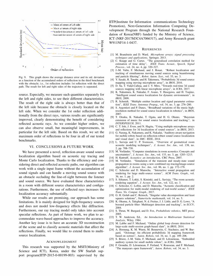
Fig. 9. This graph shows the average distance error and its std. deviationas a function of the accumulated orders of reflection in the third benchmarkwith the obstacle; i.e., 1st reflection includes 1st reflection with the directpath. The result for left and right sides of the trajectory is separated.

source. Especially, we measure such quantities separately forthe left and right sides, to see their different characteristics.The result of the right side is always better than that ofthe left side because the obstacle is closely located on theleft side. When we consider the 1st order reflection addi-tionally from the direct rays, various results are significantlyimproved, clearly demonstrating the benefit of consideringreflected acoustic rays. As we consider higher orders, wecan also observe small, but meaningful improvements, inparticular for the left side. Based on this result, we set themaximum order of reflections to be four in all of our testedbenchmarks.

VI. CONCLUSIONS & FUTURE WORK

We have presented a novel, reflection-aware sound sourcelocalization algorithm based on acoustic ray tracing andMonte Carlo localization. Thanks to the efficiency and con-sidering direct and reflected acoustic paths, our algorithm canwork with a single input frame without the accumulation ofsound signals and can handle a moving sound source withan obstacle occluding the line-of-sight between the listenerand sound source. We have evaluated these characteristicsin a room with different source characteristics and configu-rations. Furthermore, the use of reflected rays increases thelocalization accuracy substantially.

While our results are promising, our approach has somelimitations. It is mainly designed for high-frequency sourcesand does not model low-frequency effects like diffraction.Furthermore, our ray tracing model only takes into accountspecular reflections. As part of future work, we plan to ac-commodate wave-based approaches to improve the accuracy.Another key issue is to have an accurate 3D reconstructionof the scene and to classify acoustic materials that affect thereflections. Finally, we would like to extend them to multi-source localization.

ACKNOWLEDGMENT

This research was supported by the MSIT(Ministry ofScience and ICT), Korea, under the SW Starlab sup-port program(IITP-2015-0-00199-003) supervised by the

IITP(Institute for Information communications TechnologyPromotion), Next-Generation Information Computing De-velopment Program through the National Research Foun-dation of Korea(NRF) funded by the Ministry of Science,ICT (NRF-2017M3C4A7066317), and Army Research grantW911NF14-1-0437.

REFERENCES

[1] M. Brandstein and D. Ward, Microphone arrays: signal processingtechniques and applications, Springer, 2013.

[2] C. Knapp and G. Carter, “The generalized correlation method forestimation of time delay”, IEEE Trans. Acoust., Speech, SignalProcess., vol. 24, no. 4, pp. 320–327.

[3] J.-M. Valin, F. Michaud, and J. Rouat, “Robust localization andtracking of simultaneous moving sound sources using beamformingand particle filtering”, Robot. Auton. Syst., vol. 55, no. 3.

[4] Y. Sasaki, R. Tanabe, and H. Takemura, “Probabilistic 3d sound sourcemapping using moving microphone array”, in IROS, 2016.

[5] D. Su, T. Vidal-Calleja, and J. V. Miro, “Towards real-time 3d soundsources mapping with linear microphone arrays”, in ICRA, 2017.

[6] K. Nakamura, K. Nakadai, F. Asano, Y. Hasegawa, and H. Tsujino,“Intelligent sound source localization for dynamic environments”, inIROS, 2009.

[7] R. Schmidt, “Multiple emitter location and signal parameter estima-tion”, IEEE Trans. Antennas Propag., vol. 34, no. 3, pp. 276–280.

[8] S. Argentieri and P. Danes, “Broadband variations of the music high-resolution method for sound source localization in robotics”, in IROS,2007.

[9] T. Otsuka, K. Nakadai, T. Ogata, and H. G. Okuno, “Bayesianextension of music for sound source localization and tracking.”, inINTERSPEECH, 2011.

[10] C. T. Ishi, J. Even, and N. Hagita, “Using multiple microphone arraysand reflections for 3d localization of sound sources”, in IROS, 2013.

[11] G. Narang, K. Nakamura, and K. Nakadai, “Auditory-aware navigationfor mobile robots based on reflection-robust sound source localizationand visual slam”, in SMC. IEEE, 2014.

[12] L. Savioja and U. P. Svensson, “Overview of geometrical roomacoustic modeling techniques”, J. Acoust. Soc. Am., vol. 138, no.2, pp. 708–730.

[13] M. Vorlander, “Computer simulations in room acoustics: Concepts anduncertainties”, J. Acoust. Soc. Am., vol. 133, no. 3, pp. 1203–1213.

[14] H. Kuttruff, Acoustics: an introduction, CRC Press, 2007.[15] M. Vorlander, “Simulation of the transient and steady-state sound

propagation in rooms using a new combined ray-tracing/image-sourcealgorithm”, J. Acoust. Soc. Am., vol. 86, no. 1, pp. 172–178.

[16] C. Schissler and D. Manocha, “Interactive sound propagation andrendering for large multi-source scenes”, ACM Trans. Graph., vol.36, no. 1, pp. 2.

[17] S. Siltanen, T. Lokki, S. Kiminki, and L. Savioja, “The room acousticrendering equation”, J. Acoust. Soc. Am., vol. 122, no. 3.

[18] C. Schissler, C. Loftin, and D. Manocha, “Acoustic classification andoptimization for multi-modal rendering of real-world scenes”, IEEETrans. Vis. Comput. Graph., 2017.

[19] G. H. Golub and C. Reinsch, “Singular value decomposition and leastsquares solutions”, Numerische mathematik, vol. 14, no. 5.

[20] K. Okuma, A. Taleghani, N. d. Freitas, J. J. Little, and D. G. Lowe, “Aboosted particle filter: Multitarget detection and tracking”, in ECCV,2004.

[21] S. Thrun, W. Burgard, and D. Fox, Probabilistic robotics, MIT press,2005.

[22] T. W. Anderson, Ed., An Introduction to Multivariate StatisticalAnalysis, Wiley, 1984.

[23] M. Labbe and F. Michaud, “Online global loop closure detection forlarge-scale multi-session graph-based slam”, in IROS, 2014.

[24] A. Hornung, K. M. Wurm, M. Bennewitz, C. Stachniss, and W. Bur-gard, “Octomap: An efficient probabilistic 3d mapping frameworkbased on octrees”, Auton. Robots, vol. 34, no. 3, pp. 189–206.

[25] S. Briere, J.-M. Valin, F. Michaud, and D. Letourneau, “Embeddedauditory system for small mobile robots”, in ICRA, 2008.

[26] F. Grondin, D. Letourneau, F. Ferland, V. Rousseau, and F. Michaud,“The manyears open framework”, Auton. Robots, vol. 34, no. 3.