Reduction of a model of an excitable cell to a one ...medvedev/papers/physd05.pdf · Reduction of a...

Physica D 202 (2005) 37–59

Reduction of a model of an excitable cell to a one-dimensional map

Georgi S. Medvedev∗

Department of Mathematics, Drexel University, 3141 Chestnut Street, Philadelphia, PA 19104, USA

Received 13 August 2004; received in revised form 5 January 2005; accepted 27 January 2005Available online 3 March 2005

Communicated by C.K.R.T. Jones

Abstract

We use qualitative methods for singularly perturbed systems of differential equations and the principle of averaging to computethe first return map for the dynamics of a slow variable (calcium concentration) in the model of an excitable cell. The bifurcationstructure of the system with continuous time endows the map with distinct features: it is a unimodal map with a boundarylayer corresponding to the homoclinic bifurcation in the original model. This structure accounts for different periodic andaperiodic regimes and transitions between them. All parameters in the discrete system have biophysical meaning, which allowsfor precise interpretation of various dynamical patterns. Our results provide analytical explanation for the numerical studiesreported previously.© 2005 Elsevier B.V. All rights reserved.

Keywords:One-dimensional map; Singularly perturbed systems; Neurons

1. Introduction

Understanding mechanisms for patterns of electrical activity of neural cells (firing patterns) and principles fortheir selection and control is fundamental for determining how neurons function[10]. After a classical series ofpapers by Hodgkin and Huxley[18] nonlinear differential equations became the main framework for modelingneurons. The bifurcation theory for nonlinear ordinary differential equations[16,24] provides a powerful suite oftools for analyzing neuronal models. Many such models reside near multiple bifurcations. Consequently, in usingbifurcation analysis one often encounters rich and complicated bifurcation structure. Therefore, it is desirable todistinguish the universal features pertinent to a given dynamical behavior from the artifacts peculiar to a particularmodel. This is important in view of the unavoidable simplifications one makes in the process of modeling suchcomplex systems as neural cells, and under the conditions when many parameters are known approximately. The

∗ Tel.: +1 215 895 6612; fax: +1 215 895 1582.E-mail address:[email protected] (G.S. Medvedev).

0167-2789/$ – see front matter © 2005 Elsevier B.V. All rights reserved.doi:10.1016/j.physd.2005.01.021

38 G.S. Medvedev / Physica D 202 (2005) 37–59

goal of the present paper is to describe some general traits of the bifurcation structure of a class of models ofbursting neurons. They follow from the generic properties of two-dimensional flows near a homoclinic bifurcation.We present a method of reduction of a model of an excitable cell to a one-dimensional map. The bifurcation structureof the system with continuous time endows the map with distinct features: it is a unimodal map with a boundarylayer corresponding to the homoclinic bifurcation in the original model. The qualitative features of this map accountfor periodic and aperiodic regimes and transitions between them. Our analytical results are consistent with thenumerical results reported in the literature[6,7], which, in turn, reflect many salient features of the experimentaldata. Our approach in this paper is to describe general features of the bifurcation structure of the problem: we do notpursue the study of the fine structure in the (small) parameter windows of complex and possibly chaotic dynamics.We believe that more detailed information in these windows in the parameter space can be obtained using ourmethod. We think that the level of detail we achieve gives a comprehensive picture of the bifurcation structure ofthe problem, while keeping the analysis simple. Our approach retains the biophysical meaning of the parameters inthe process of reduction, which allows for precise interpretation of various dynamical patterns.

To illustrate our approach we choose a three-variable model of an excitable cell introduced by Chay[6]. Themodel in [6] is a unified model for both the neuronal and secretory excitable membranes[8,39–41]. We shallrefer to it as the Chay model. It captures many features of a more detailed physiological model of a pancreatic�-cell, the Chay–Keizer model[8]. In addition to providing a mathematical description for a complex and importantphysiological system (�-cells of the pancreas secrete insulin, a hormone that maintains the glucose blood levelwithin narrow range), it captures several essential features common to many other models of bursting neurons. Inthis respect, we mention models of pyramidal cells in the neocortex[47,48], thalamic cells[32,37]and those of cellsin the pre-Botzinger complex involved in the control of respiration[5]. These models possess similar dynamicalmechanisms for bursting, although the ionic bases may be different. Another interesting feature of the Chay modelis that it nicely illustrates the mechanism, by which calcium current controls the modes of activity in neural cells.We show that the variation of the maximal conductance of the voltage-dependent calcium current results in thetransition from tonic spiking to bursting, as well as in the transitions between various bursting regimes (Fig. 1).Therefore, our results may be relevant to other models of neural cells involving calcium dynamics.

Bursting oscillations are ubiquitous in the experimental and modeling studies of excitable cells (see[5,8,10,13,14,32,37,39–41,47–49]and references therein). Biological significance and dynamical complexity ofbursting oscillations stimulated mathematical investigations of the mechanisms of bursting behaviors[1,3,6,7,9,12–15,17,19,20,30,31,33–35,42,43,45,46,49,51]. Even minimal 3D models of bursting neurons exhibit a variety ofperiodic and aperiodic regimes under the variation of parameters. In particular, windows of chaotic dynamics wereidentified in the transitions from tonic spiking to bursting and in between different bursting regimes in a class ofmodels of excitable membranes[1,6,7,9,34]. In [45,46], Terman rigorously showed the existence of chaotic regimesin a three-variable model of a bursting neuron. The analyses in[45,46] used 2D flow-defined maps near a homo-clinic connection. Belykh et al.[3] proposed several mechanisms for the onset of bursting using 2D flow-definedmaps. Recent studies of the transitions from bursting to continuous spiking in[42,43]showed that such transitionsmay involve highly nontrivial bifurcation scenarios such as the blue-sky catastrophe and the Lukyanov–Shilnikovbifurcations. Therefore, a comprehensive description of the dynamical phenomena associated with the transitionsbetween different periodic regimes in the models of bursting neurons presents a challenging problem. Our studyis motivated by numerical results showing that one-dimensional first return maps constructed for the slow variableaccount for various periodic and aperiodic regimes in a class of models. This approach was used in[1,6,7,34]toexplain the origins of the chaotic dynamics in certain models. One-dimensional maps provide a valuable tool forstudying oscillatory dynamics in a variety of biological and physical models (see, e.g.,[22,25,26,28,38,44,52]). Inthe present paper, our goal was to derive the first return map for the dynamics of the slow variable in the Chay modeland to study its properties analytically. Our approach is similar to that used by Rinzel and Troy in their studies ofthe bursting patterns in a model for the Belousov–Zhabotinsky reaction[35,36]. In [27], we used a similar approachto analyze the bifurcation structure of the family of mixed-mode periodic solutions for a compartmental model ofthe dopamine neuron. As in[27], the first return map for the Chay model is computed using two functions of cal-

G.S. Medvedev / Physica D 202 (2005) 37–59 39

cium concentration: the period of oscillations and the average value of the voltage-dependent calcium current whenthe concentration of calcium is kept constant. We were able to obtain detailed information about these functionsusing the results from the geometric theory for differential equations[21,23]and bifurcation theory[16,24]. For allpractical purposes, these functions can be computed numerically. The latter approach may be useful in analyzinghigher dimensional models, for which analytical methods may not be available. We also envision that in certaincases these functions can be evaluated directly from the experimental data. We believe that our approach will beuseful for understanding mechanisms for firing patterns in a broad class of models.

The outline of the paper is as follows. In Section2, we describe the Chay model and present numerical examplesof the different spiking and bursting patterns generated by the model. Following[34], we identify the fast and theslow subsystems by separating timescales. Section3 contains the bifurcation analysis of the two-dimensional fastsubsystem. We show that under the variation of the control parameter, the fast subsystem undergoes a supercriticalAndronov–Hopf (AH) bifurcation, followed by a saddle-node (SN) bifurcation and a homoclinic (HC) bifurcation.This information is used in Section4, where we derive a one-dimensional first return map for the slow variable,the concentration of calcium. In Section5, we analyze the bifurcations in a one-parameter family of the first returnmaps and relate them to the transitions between different spiking and bursting regimes. Finally, several naturalgeneralizations of our results are given in Section6.

2. The model

The model in[6] describes the dynamics of the membrane potential,v(t), and calcium concentration,u(t), in acell with voltage-dependent sodium, potassium, and calcium channels, and calcium-dependent potassium channels:

dv

dt= gIm

3∞(v)h∞(v)(EI − vt) + gKVn

4(EK − v) + gKCu

1 + u(EK − v) + gL(El − v), (2.1)

dn

dt= n∞(v) − n

τ(v), (2.2)

du

dt= ρ(m3

∞(v)h∞(v)(ECa − v) − γu). (2.3)

The first equation is the current balance equation, where the first term models effective conductance through thecalcium and sodium channels. The activation of the voltage-dependent potassium channels changes according to(2.2). The calcium dynamics is modeled by the last equation. The intracellular calcium concentration,u(t), is scaledby its dissociation constant and is a nondimensional variable. To have a better picture of the timescales associatedwith Eqs.(2.1)–(2.3), we rescalev andt: v = kvv andt = ktt, wherekv = 10 mV andkt = 1/230 s−1. Using thesechanges of variables and by dividing both sides of(2.1)by gKV we obtain the following system of equations:

εv = am3∞(v)h∞(v)(EI − v) + n4(EK − v) + δu

1 + u(EK − v) + l(El − v), (2.4)

n = n∞(v) − n

τ(v), (2.5)

u = α(γ−1m3∞(v)h∞(v)(ECa − v) − u), (2.6)

where

ε = (gKVkt)−1, a = gI

gKV, l = gL

gKV, α = ργ, γ = γ

kv, ρ = ρkvkt, and δ = gKC

gKV.


Fig. 1. Plots of the time series ofv(t) for different values ofgKC demonstrate several firing patterns generated by(2.1)–(2.3): rhythmic singlespiking, doublets, irregular and rhythmic bursting.

For the values of parameters of the original model(2.1)–(2.3)we refer to[6]. In Appendix A, we present theparameter values for the nondimensional model(2.4)–(2.6)and the analytical expressions for the functionsm∞,h∞, n∞, andτ. The latter have typical sigmoid forms similar to the corresponding functions in the Hodgkin–Huxleymodel. In[6], it was shown numerically that by varyinggKC in the range 10–30 s−1, system of equations(2.1)–(2.3)has a variety of periodic and chaotic spiking and bursting solutions (Fig. 1). Following [6], we shall study thebifurcations of the periodic solutions of(2.4)–(2.6), usingδ as a control parameter.

Remark 2.1. It is interesting to note that the coefficients in front of the first two terms on the right-hand side of(2.4) are close to 1, whereas the last two terms have coefficients∼10−3 to 10−2. Since the system of equations(2.4)–(2.6) is close to several bifurcations, the smaller terms are significant on the scale set by the distance of thesystem to the closest bifurcation in the parameter space. Therefore, they cannot be neglected.

System(2.4)–(2.6) is a singularly perturbed system of equations[21,29]. Our analysis uses the disparatetimescales of the system dynamics, which are set by the small positive parametersα andε. Specifically, we separatethe equations in(2.4)–(2.6)into the fastandslow subsystems. The former is obtained by viewingu in (2.4) and


(2.5)as a parameter, i.e., by formally settingα = 0:

εv = am3∞(v)h∞(v)(EK − v) + n4(EK − v) + δu

1 + u(EK − v) + l(El − v), (2.7)

n = n∞(v) − n

τ(v). (2.8)

The remaining equation(2.6) forms the slow subsystem. Below we show that in the range of parameters of interestthe fast subsystems generates oscillations inv. Therefore, Eq.(2.6) is in the form suitable for application of themethod of averaging[4,16]. In Section4, we derive a map for the change inu after one cycle of oscillations of thefast subsystem:

u = P(u). (2.9)

The study of the dynamics and bifurcations in the original system(2.1)–(2.3)is then reduced to the analysis of theone-dimensional map(2.9).

3. Analysis of the fast subsystem

In the present section, we use phase plane techniques to determine the bifurcations in(2.7)and(2.8)under thevariation of

β = δu

1 + u, (3.1)

whereu is fixed. It turns out that the system resides in the vicinity of the two bifurcations: a supercritical AHbifurcation and a HC bifurcation. Near these bifurcations the properties of the periodic orbits follow from the well-known results of the bifurcation theory[16,24]. We use this information in the next section to obtain the qualitativeproperties of the map in(2.9)and to determine the bifurcations of(2.9)under the variation ofδ.

The fast subsystem is in turn a singularly perturbed system of two equations. For smallε > 0, the dynamicsof (2.7) and(2.8) can be deduced using the geometric methods for singularly perturbed systems[21,29]. For 2Dsystems, such as(2.7)and(2.8), a great deal of information can be obtained from the nullcline configuration in thephase plane. Thev- (n-)nullcline in the phase plane of(2.7)and(2.8) is the set of points wherev (n) vanishes. Bysetting the right-hand sides of the Eqs.(2.7) and (2.8)to zero, we obtain the equations for the nullclines:

n4 = am3∞(v)h∞(v)(EI − v) + l (El − v)

v− EK− β and n = n∞(v), (3.2)

whereβ is defined in(3.1).In the range of parameters of interest equations in(3.2) define two curves in then–v plane. Note that inn4–v

plane the variation ofβ results in a simple translation of thev-nullcline in vertical direction. Using this observation,we determine the following sequence of events:

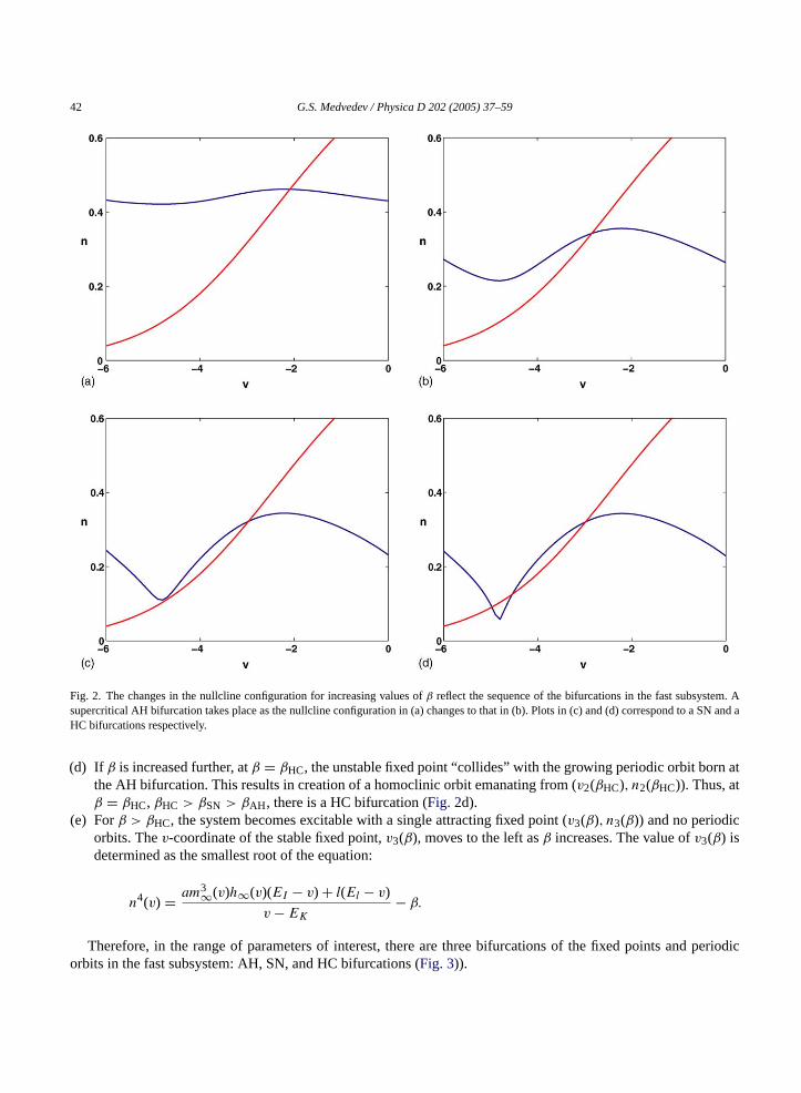
(a) For negative values ofβ near 0, the nullclines intersect at a single point (v1(β), n1(β)), n1(β) = n∞(v1(β)).Since the point of intersection lies to the right of the point of maximum of thev-nullcline (i.e., on the stablebranch of the slow manifold of(2.7) and (2.8)), it is a stable fixed point (Fig. 2a).

(b) Asβ increases, thev-nullcline moves down andv1(β) moves to the left. After it passes the point of the maximumof thev-nullcline,vmax, there is a supercritical AH bifurcation atβ = βAH (Fig. 2b).

(c) Asβ increases further, the lower knee of thev-nullcline touches then-nullcline atβ = βSN. This corresponds to asaddle-node (SN) bifurcation. It creates two fixed points: (v2(β), n2(β)) and (v3(β), n3(β)), n2,3 = n∞(v2,3(β)),v2(β) > v3(β). The former is unstable and is moving to the right for increasingβ (Fig. 2c).


Fig. 2. The changes in the nullcline configuration for increasing values ofβ reflect the sequence of the bifurcations in the fast subsystem. Asupercritical AH bifurcation takes place as the nullcline configuration in (a) changes to that in (b). Plots in (c) and (d) correspond to a SN and aHC bifurcations respectively.

(d) If β is increased further, atβ = βHC, the unstable fixed point “collides” with the growing periodic orbit born atthe AH bifurcation. This results in creation of a homoclinic orbit emanating from (v2(βHC), n2(βHC)). Thus, atβ = βHC, βHC > βSN > βAH, there is a HC bifurcation (Fig. 2d).

(e) Forβ > βHC, the system becomes excitable with a single attracting fixed point (v3(β), n3(β)) and no periodicorbits. Thev-coordinate of the stable fixed point,v3(β), moves to the left asβ increases. The value ofv3(β) isdetermined as the smallest root of the equation:

n4(v) = am3∞(v)h∞(v)(EI − v) + l(El − v)

v− EK− β.

Therefore, in the range of parameters of interest, there are three bifurcations of the fixed points and periodicorbits in the fast subsystem: AH, SN, and HC bifurcations (Fig. 3)).


Fig. 3. The bifurcation diagram for the fast subsystem(2.7) and (2.8). The dotted line corresponds to the minimal values ofv(t) taken on theperiodic orbits from the family of solutions born at the AH bifurcation and terminated at the HC bifurcation. The S-shaped curve correspondsto a curve of fixed points. For computational convenience, we usedu as a bifurcation parameter to generate this diagram. Clearly, the diagramdoes not change qualitatively, if one usesβ as a control parameter instead ofu, becauseβ is a monotone function ofu.

Remark 3.1.

(a) The bifurcation diagram inFig. 3was obtained with numerical continuation software XPPAUT[11]. However,the qualitative form of this bifurcation diagram follows from the considerations presented in (a)–(e). Moreover,the values ofβAH andβSN can be estimated analytically, using standard methods of the bifurcation theory[16,24]. We do not perform these calculations, because the qualitative information obtained with the phaseplane analysis is sufficient for our purposes.

(b) The family of periodic orbits emanating from the AH bifurcation may undergo a saddle-node of limit cyclesbifurcation before it limits onto the branch of equilibria. This situation is discussed inSection 6. In the mainpart of the paper, we assume that the limit cycles retain stability up to the HC bifurcation atβ = βHC.

For construction of map(2.9), we need to review some properties of periodic orbits near a supercritical AH andHC bifurcations. In 2D singularly perturbed systems, such as(2.7) and (2.8), a periodic orbit born at a supercriticalAH bifurcation undergoes a canard transition in a neighborhood of the AH bifurcation[23]. This transition isdetermined by the local vector field near the AH bifurcation point. For sufficiently smallε → 0, Theorem 3.3 in[23] implies the following properties of the canard cycles:

(C0) Forβ > βAH and close toβAH, there is a unique limit cycleZβ(ε), which converges to a singular cycleZβ inHausdorff metric, asε → 0. The shape ofZβ is determined by thev-nullcline (3.2)as shown inFig. 4a.

(C1) In addition, if the conditions of Theorem 3.4 of[23] are satisfied, the canard cyclesZβ are asymptoticallystable and their amplitudes grow monotonically withβ. Here we refer to the condition involving the “way-in–way-out” function (Theorem 3.4 of[23]). This condition can be verified by a straightforward albeit tediouscalculation. For all practical purposes, it can be easily checked numerically. Henceforth, we assume that thiscondition holds for(2.7) and (2.8).

Remark 3.2. Although for the value ofε ∼ 0.1, used in the Chay model, the periodic trajectories substantiallydeviate from those in the singular limitε → 0, the qualitative features of the family of periodic orbits are capturedby the family of singular trajectories. Alternatively, this family can be described by viewing the fast subsystem as a


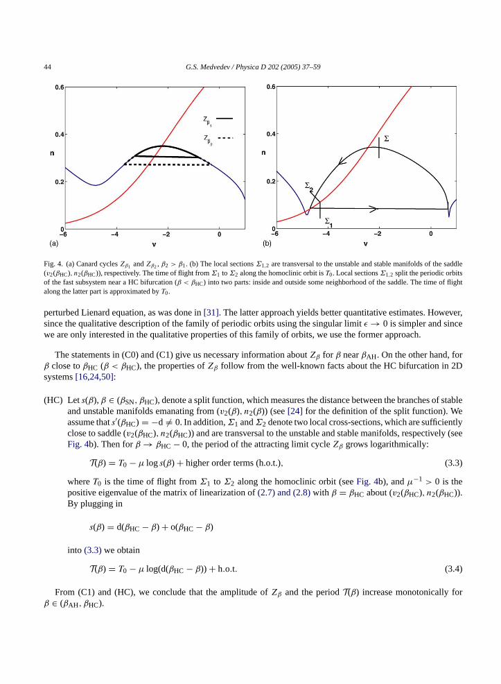
Fig. 4. (a) Canard cyclesZβ1 andZβ2, β2 > β1. (b) The local sectionsΣ1,2 are transversal to the unstable and stable manifolds of the saddle(v2(βHC), n2(βHC)), respectively. The time of flight fromΣ1 toΣ2 along the homoclinic orbit isT0. Local sectionsΣ1,2 split the periodic orbitsof the fast subsystem near a HC bifurcation (β < βHC) into two parts: inside and outside some neighborhood of the saddle. The time of flightalong the latter part is approximated byT0.

perturbed Lienard equation, as was done in[31]. The latter approach yields better quantitative estimates. However,since the qualitative description of the family of periodic orbits using the singular limitε → 0 is simpler and sincewe are only interested in the qualitative properties of this family of orbits, we use the former approach.

The statements in (C0) and (C1) give us necessary information aboutZβ for β nearβAH. On the other hand, forβ close toβHC (β < βHC), the properties ofZβ follow from the well-known facts about the HC bifurcation in 2Dsystems[16,24,50]:

(HC) Lets(β), β ∈ (βSN, βHC), denote a split function, which measures the distance between the branches of stableand unstable manifolds emanating from (v2(β), n2(β)) (see[24] for the definition of the split function). Weassume thats′(βHC) = −d = 0. In addition,Σ1 andΣ2 denote two local cross-sections, which are sufficientlyclose to saddle (v2(βHC), n2(βHC)) and are transversal to the unstable and stable manifolds, respectively (seeFig. 4b). Then forβ → βHC − 0, the period of the attracting limit cycleZβ grows logarithmically:

T(β) = T0 − µ logs(β) + higher order terms (h.o.t.), (3.3)

whereT0 is the time of flight fromΣ1 to Σ2 along the homoclinic orbit (seeFig. 4b), andµ−1 > 0 is thepositive eigenvalue of the matrix of linearization of(2.7) and (2.8)with β = βHC about (v2(βHC), n2(βHC)).By plugging in

s(β) = d(βHC − β) + o(βHC − β)

into (3.3)we obtain

T(β) = T0 − µ log(d(βHC − β)) + h.o.t. (3.4)

From (C1) and (HC), we conclude that the amplitude ofZβ and the periodT(β) increase monotonically forβ ∈ (βAH, βHC).


4. The first return map

Our goal in the present section is to derive a first return map for the dynamics of slow variableu, calciumconcentration. We denote the first return map by

u = P(u) (4.1)

and give a precise definition ofP below. MapP(u) reflects the changes of the calcium concentration after distinctevents in the dynamics of the fast subsystem. Specifically, it shows how each spike within a burst affects the calciumconcentration and how the latter changes after the period of quiescence. In the previous section, we identified thebifurcation structure of the fast subsystem and described the qualitative features of the family of periodic orbits,which supports spiking and bursting behaviors of the full 3D model(2.4)–(2.6). In particular, we showed thatthe period of oscillationsT(β) is a monotone function tending to∞, asβ → βHC − 0. These properties naturallytranslate into the qualitative form of the first return map. Our main observation about the structure ofP is that itsdomain of definition can be split into three regions according to the qualitative form ofP. These are the left-outerregion,I−, the inner region,I0, and the right-outer region,I+ (Fig. 5). The form ofP in each of these regionsreflects the properties of the attractors in the fast subsystem before, near, and past the HC bifurcation. A typicalexample ofP is shown inFig. 5. An examination ofFig. 5 shows that in the left-outer region,I−, P is close toa linear map with the slope slightly less than 1. The iterations ofP in I− form an increasing sequence, whichcorresponds to a monotone increase in the calcium concentration during a burst. In the right-outer region,I+, P isapproximately constant (see also Remark 5.3b). The value ofP in I+ corresponds to the calcium concentration atthe end of the quiescent phase. The structure ofP in the boundary layerI0 is determined by the properties of theperiodic orbits of the fast subsystem near the HC bifurcation. We show that, inI0, P is unimodal with the slopetending to−∞ at the border betweenI0 andI+. This information about the qualitative form ofPwill be useful inSection6, where we study the bifurcations of the fixed point and stable periodic orbits in a family of discrete 1Ddynamical systems(4.1). In Section6, we will also relate the results of the bifurcation analysis for(4.1) to spikingand bursting regimes of the original system of ordinary differential equations(2.4)–(2.6)and to transitions betweenthem.

Fig. 5. Three regions in the domain of definition ofP: the left-outer region,I−, the inner region,I0, and the right-outer region,I+.


After these preliminary remarks we proceed with the derivation of the first return map. First, we make ourdefinition ofP precise. For this, we need the following auxiliary definitions:

uy = βy

δ− βy, y ∈ {AH,HC,SN}, (4.2)

T (u) = T(β), whereβ = δu

1 + u.

In then–v plane we take a local sectionΣ, which is transversal to thev-nullcline, as shown inFig. 4b. As before, byZβ, βAH < β < βHC we denote singular canard cycles lying inside the homoclinic orbit. Letξ ∈ (uAH, uHC) and(v0, n0) = Σ ∩ Zβ, with β = δξ(1 + ξ)−1. Next we integrate(2.4)–(2.6)with initial condition (v0, n0, ξ). MapP isdefined by

P(ξ) = u(T (ξ)),

whereT (ξ) is the time of the first return, i.e.,

T (ξ) = min{t > 0 : (v(t), n(t)) ∈ Σ andφ(t) · e2 < 0}, φ(t) = (v(t), n(t)), e2 = (0,1),

and· denotes the scalar multiplication inR2.From(2.6)we have

P(ξ) = e−αT (ξ)ξ + ρ

∫ T (ξ)

0f (v(s)) eα(s−T (ξ)) ds, (4.3)

whereρ = αγ−1 and

f (v) = m3∞(v)h∞(v)(ECa − v).

We rewrite(4.3)as

P(ξ) = e−αT (ξ)ξ + ρf (ξ)∫ T (ξ)

0eα(s−T (ξ)) ds = e−αT (ξ)ξ + (1 − e−αT (ξ))F (ξ), (4.4)

where

f (ξ) =∫ T (ξ)

0 f (v(s)) eα(s−T (ξ)) ds∫ T (ξ)0 eα(s−T (ξ)) ds

and F (ξ) = f (ξ)

γ.

The structure of map(4.4) is determined by two functions of calcium concentration: the period of oscillations,T (ξ), and the weighted average amount of calcium entering the cell with the voltage-dependent calcium currentduring one cycle of oscillations scaled by the calcium removal constant,F (ξ). Note thatF (ξ) must be O(1) in thecontext of this model, because it represents the ratio of the rate of the voltage-dependent calcium current and thatof its removal. If one of these quantities is significantly bigger than the other, the calcium dynamics will be trivial.Near the HC bifurcation, the period of oscillations of the fast system changes drastically. This creates three regionsin the domain of definition ofP, over which it has qualitatively different form. To introduce these regions, we


define

u0 = β0

δ− β0, whereβ0 : T(β0) = T0,

whereT0 is defined in(3.3).We distinguish the following regions in the domain of definition ofP:

(a) The left-outer region: I− = [0, u0].By continuous dependence of solutions of(2.4)–(2.6)onα, for ξ ∈ I−, we have

T (ξ) = T0(ξ) + O(α), (4.5)

(v(t), n(t)) = (v0(t), n0(t)) + O(α), 0 ≤ t ≤ T (ξ), (4.6)

where (v0(t), n0(t)), t > 0 is the periodic solution of the fast subsystem with initial condition (v0, n0) andu = ξ

andT0(ξ) is its period. By plugging in(4.5) and (4.6)into (4.4) and using the Taylor’s expansion for theexponential function, we obtain

P(ξ) = (1 − αT0(ξ))ξ + αT0(ξ)F (ξ) + O(α2), ξ ∈ I−. (4.7)

Therefore, in the left-outer region, for sufficiently smallα, P(ξ) is close to a linear map with a positive slopeless than 1 (seeFig. 5).

(b) The inner region: I0 = [u0, uHC].In the inner region, the period of oscillations of the fast subsystem(2.7) and (2.8),T0(ξ) grows without bound.

To obtain a uniform approximation of the trajectory of (v(t), n(t), u(t)) for ξ ∈ I0. We modify the constructionof the first return map. In then–v plane we use two sectionsΣ1 andΣ2 that divide the periodic orbits of thefast subsystem near the HC bifurcation into two parts (seeFig. 4b):(1) The portion lying outside a neighborhood of the homoclinic point (vHC, nHC), wherevHC = v2(βHC), nHC =

n∞(vHC). The time of flight of the phase point of the fast subsystem along this portion of the periodic orbitto leading order does not depend onu and is approximately equal toT0, the time of flight along thecorresponding portion of the homoclinic orbit foru = uHC.

(2) The remaining part of the periodic orbit lies in a small neighborhood of (vHC, nHC).As before, we defineP1 : R → R by taking the initial condition (v0, n0, ξ) such that (v0, n0) ∈ Zβ ∩Σ1,

β = δξ(1 + ξ)−1 and integrating(2.4)–(2.6)until the projection of the trajectory to thev–n plane hitsΣ2 at timet = T1(ξ). We defineP1(ξ) = u(T1(ξ)). Similarly, we defineP2 by taking the initial condition whose projectionontov–n lies inΣ2 and integrating(2.4)–(2.6)until the projection of the phase trajectory hitsΣ1. Finally, wedefineP = P2 ◦ P1.P1 is computed as in(4.7):

P1(ξ) = (1 − αT0)ξ + αT0F0 + O(α2), F0 = 1

γT0

∫ T0

0f (v(s)) eα(s−T0) ds. (4.8)

Let ξ1 = P1(ξ). To computeP2, we rewrite(3.4):

T (ξ1) − T0 = −µ log

(d

(βHC − δξ1

1 + ξ1

))+ h.o.t. (4.9)

From(4.3)we have

P2(ξ1) = e−α(T (ξ1)−T0)ξ1 + ρ

∫ T (ξ1)

T0

f (v(s)) eα(s−T (ξ1)) ds. (4.10)


Note that, by(4.9),

e−α(T (ξ1)−T0) = C(α)

(βHC − δξ1

1 + ξ1

)αµ, whereC(α) = dαµ(1 + o(1)) → 1 asα → 0. (4.11)

∫ T (ξ1)

T0

f (v(s)) eα(s−T (ξ1)) ds ≈ f (vHC)∫ T (ξ1)

T0

eα(s−T (ξ1)) ds

= α−1f (vHC)

(1 − C(α)

(βHC − δξ1

1 + ξ1

)αµ). (4.12)

By combining(4.10)–(4.12), we obtain

P2(ξ1) = C(α)

(βHC − δξ1

1 + ξ1

)αµ(ξ1 − F1) + F1 + h.o.t., whereF1 = f (vHC)γ−1. (4.13)

Note that, by(4.10) and (4.13),

P2(ξ) ={ξ asξ → u0 + 0,

F1 asξ → uHC − 0.

Therefore, we have continuously extendedP from the left-outer region through the inner region.(c) Finally, we definethe right-outer regionfor ξ > uHC. For this, we recall that foru > uHC, all trajectories of the

fast subsystem (except that starting from the unstable fixed points) converge to a unique attracting equilibrium(v3(β), n3(β)), β = δu(1 + u)−1 (see Statement (e), Section3). This observation combined with(2.6)yields

u = α(γ−1f (ψ(u)) − u), (4.14)

whereψ(u) = v3(β), β = δu(1 + u)−1. Using an argument commonly applied in the analysis of bursting[34],one shows that (v3(u), n3(u)) moves close to the stable branch of the fixed points parameterized byu, asu isslowly decreasing according to(4.14)until it reachesu = uSN. Therefore, we extend the definition ofP(ξ) forξ > uHC by

P(ξ) = uSN < uHC. (4.15)

The last inequality follows from statements (c) and (d) of the previous section.

This completes the description of the first return mapP.

5. Bifurcations of the first return map

In the present section, we study the bifurcations of the stable solutions of(2.4)–(2.6)under the variation ofδ(or, in terms of the original system(2.1)–(2.3), for varyinggKC). The analysis of the previous section reduces thisproblem to the study of bifurcations in a one-parameter family of maps(4.1). A heuristic examination ofP suggeststhat there are two main types of attractors of(4.1): a stable fixed point and a superstable cycle (seeFig. 5). Clearly,these two types of attractors of the discrete system correspond to spiking and bursting patterns generated by theoriginal system(2.4)–(2.6). Our approach in this section is to locate a unique fixed point ofPand to track its positionunder the variation ofδ. In particular, we show that for small values ofδ, the fixed point lies in the left-outer region,where it is necessarily stable, because the slope of the graph ofP(u) in I− is less than 1. Ifδ is increased, the fixedpoint moves into the inner region. By following the fixed point as it moves through the inner region, we detect


the main events in the sequence of bifurcations of the discrete system. The first bifurcation in this sequence is aperiod-doubling (PD) bifurcation of the fixed point, which gives rise to a two-spike periodic solution (a doublet) ofthe continuous system(2.4)–(2.6)(seeFig. 1b). For larger values ofδ, there exists a family of superstable cyclesof P, which correspond to bursting solutions of the original system. For a piecewise-linear approximation ofP, weshow that the family of superstable cycles undergoes reverse period-adding bifurcations for increasing values ofδ.This implies the order, in which different bursting solutions appear in the continuous system under the variation ofcontrol parameter. Finally, we comment on the possibility of complex dynamics in narrow windows in the parameterspace lying between regions of existence of distinct bursting solutions. Therefore, the results of this section providea comprehensive description of stable periodic solutions of the original system(2.4)–(2.6)and suggest mechanismsfor transitions between them.

First, we show that there exists a unique fixed point ofP in the range of parameters of interest and clarify itsdependence on the control parameterδ. From(4.4), we obtain the equation for the fixed points ofP:

F (u) = u. (5.1)

It is convenient to rewrite this equation in terms ofβ:

F(β) = β

δ− β, whereF(β) ≡ F

(β

δ− β

). (5.2)

As shown inAppendix B, functionF(β) has the following properties:

(a) F(β) is a decreasing continuous function on [0, βHC] with F(βHC − 0) = F1,(b) F′(βHC − 0) = −∞.

In the remainder of this section, we will need the following definitions:

β0 : T(β0) = T0, δ0 :β0

δ0 − β0= F(β0), i.e., δ0 = β0(1 + F(β0)−1), (5.3)

δ :βHC

δ− βHC= F(βHC), i.e., δ = βHC(1 + F(βHC)−1) (5.4)

(seeFig. 6).

Fig. 6. The graphs ofF(β) (solid line) and functions on the left-hand sides of(5.3) and (5.4)(dashed and dash-dotted lines, respectively).


Fig. 7. The plots ofP for two values ofδ : δ1 < δ2. Plots in (a) and (b) show the fixed point ofP before and after the PD bifurcation.

5.1. The fixed point of P: regular spiking

Using monotonicity of functions on the both sides of(5.2), we conclude that(5.2) has a unique solution on[0, βHC] provided

F(βHC) ≤ βHC

δ− βHC(or F (uHC) ≤ uHC). (5.5)

This implies that there is a unique solutionβ(δ) of (5.2) for 0 ≤ δ ≤ δ. β(δ) is a continuous increasing function on[0, δ] andβ(δ) → βHC asδ → δ− 0. Therefore, forδ ∈ [0, δ], Phas a unique fixed point ¯u(δ) ∈ [0, uHC]. Moreover,for δ ∈ [0, δ0] the fixed point lies in the left-outer region. It is easy to see that ¯u(δ) is attracting in this case.

Remark 5.1. Inequality(5.5)gives a sufficient condition for the oscillatory activity (both spiking and bursting) in(2.4)–(2.6). It has a simple biophysical interpretation:(5.5) requires that the voltage-dependent calcium current isdominated by the removal of calcium when calcium concentration is kept constant atu = uHC.

5.2. The period-doubling bifurcation: firing in doublets

As δ is increased fromδ0 to δ, the fixed point moves through the inner region. Below we show that it loosesstability through a PD bifurcation at a certain value of control parameterδ = δPD ∈ (δ0, δ) (Fig. 7). In terms ofperiodic solutions of continuous system(2.4)–(2.6), the PD bifurcation corresponds to the birth of a doublet, atwo-spike periodic solution (seeFig. 1b).

By differentiating(4.4), we have

P ′(u) = αT ′(u) e−αT (u)(F (u) − u) + e−αT (u) + F ′(u)(1 − e−αT (u)).

To locate the PD bifurcation of ¯u(δ), we set the derivative ofP at u(δ) to −1:

P ′(u(δ)) = e−αT (u(δ)) + F ′(u(δ))(1 − e−αT (u(δ))) = −1. (5.6)

In the equation above, we used(5.1) to simplify the expression forP ′(u). Next, we show that(5.6) has a so-lution in (δ0, δ). For this, we note that forδ varying from δ0 to δ, the fixed point ¯u(δ) moves fromu0 to uHC.


In addition,

P ′(u(δ0)) = P ′(u0) = e−αT0 + F ′(u0)(1 − e−αT0) = 1 − αT0 + αF ′(u0)T0 + O(α2) = 1 + O(α) > −1.

(5.7)

On the other hand, asδ → δ− 0, u(δ) → uHC − 0. By takingδ → δ− 0 in the expression ofP ′(u(δ)) in (5.6), weobtain

P ′(u(δ− 0)) = P ′(uHC − 0) = −∞ < −1, (5.8)

because limu→uHC−0 e−αT (u) = 0 and limu→uHC−0 F′(u) = −∞. By combining(5.6)–(5.8), we conclude that(5.6)

has a solution on (δ0, δ). We denote the smallest solution of(5.6)on (δ0, δ) by δPD. Therefore, ¯u(δ) is attracting forδ ∈ (0, δPD), δPD < δ, and it undergoes a PD bifurcation atδ = δPD. The attracting period 2 cycle born at the PDbifurcation corresponds to a doublet solution of the original model(2.4)–(2.6)(Fig. 1b).

5.3. Superstable cycles of P: bursting

In the present section, we show that for sufficiently largeδ ∈ (δ0, δ), the first return mapP has a family ofsuperstable cycles, which correspond to bursting periodic solutions of continuous system(2.4)–(2.6). By studyingthe bifurcations of the cycles of discrete system we establish the order, in which the bursting patterns appear incontinuous system(2.4)–(2.6)for increasing values of control parameter.

Bursting is generated by the first return maps whose iterations revisit the right-outer region,I+. By regular(periodic) bursting we refer to superstable cycles ofP of the form:

Sq = {xi, i = 1,2, . . . , q+ 1 : x1 = P(uSN), xq > uSN, xj+1 = P(xj), j = 1,2, . . . , q− 1}.

A necessary and sufficient condition for regular bursting is given by

∃k ∈ Z+ : Pk(uSN) ∈ J1,

whereJ1 = {u : P(u) > uHC}. We shall use the following observation:

(B) There existsδb ∈ (0, δ) such that maxu∈[0,uHC] P(u) > uHC for δ ∈ (δb, δ).

Indeed, as we showed in Section5.1, the fixed point ofP, u(δ) → uHC asδ → δ− 0. On the other hand, by(5.8),P ′(u) → −∞ asδ → δ− 0. Therefore, statement in (B) holds.

From (B) we conclude thatJ1 = ∅ for δ ∈ (δb, δ). We decompose the inner region,I0, into three closed intervals:

I0 = J0 ∪ J1 ∪ J2, i = j, Ji ∩ Jj = ∅, i, j ∈ {0,1,2},

where open intervalJ0(J2) lies to the left (right) ofJ1. Note that the remarks following (B) imply that the size ofJ2 tends to zero asδ → δ− 0 (compareFig. 8a and b). Henceforth, we shall assume thatδ ∈ (δb, δ) is sufficientlyclose toδ so that the size ofJ2 is sufficiently small. Our numerical results suggest that these assumptions holdfor the most part of the interval inδ (gKC) corresponding to bursting behavior in the Chay model (seeFig. 8b).Furthermore, the numerics gives a clear evidence that onI0 ∪ J0, P can be approximated well by a linear function.For such approximation, we choose

Pl(u) = Au+ αF0T0, whereA = 1 − αT0. (5.9)


Fig. 8. The bursting patterns exhibit reverse period-adding for increasing values ofgKC.

Remark 5.2. Note that we only need thatPl be close toP on I− ∪ J0, because onJ1 the definition ofPl isirrelevant, as long asPl(u) > uHC, andJ2 is very small. It can be shown that onI−, P andPl are O(α) closein C1-metric (see(4.7)). This statement can be extended toJ0 provided thatJ0 lies sufficiently far away foruHC.

We extend the definition ofPl to the rest of the inner region:

Pl(u) ={Au+ αF0T0, I

− ∪ I0,

uSN, I+.(5.10)

With the assumptions that we made earlier, we reduce the study of the superstable cycles ofP to those ofPl. Forsufficiently smallα > 0, the implicit function theorem implies the existence of a superstable cycleSq ofPwheneverPl has a superstable cycleSq bounded away fromJ2.

To study the superstable cycles ofPl we note that

Pk(uSN) = AkuSN + αT0F0(Ak−1 + Ak−2 + · · · + 1) = (1 − kαT0)uSN + kαT0F0 + O(α2). (5.11)


Therefore, the region of existence of a superstable cycleSk of Pl is given byδk ≤ δ < δk−1, where

δk : Pkl (uSN) = uHC for δ = δk. (5.12)

Using(4.2) and (5.11), we rewrite(5.12)as follows:

(1 − kαT0)βSN

δk − βSN+ kαT0F0 = βHC

δk − βHC+ h.o.t. (5.13)

From(5.13)we obtain

δk = βSN(1 + F0) + βHC − βSN

αkT0· δk

δk − βHC+ h.o.t. (5.14)

By taking into account thatδ ∈ (0.01,0.02) andβHC ≈ 2.03× 10−3, we approximate

δk

δk − βHC≈ 1

and obtain

δk ≈ βSN(1 + F0) + βHC − βSN

αkT0. (5.15)

The last expression implies that the family superstable cycles of the piecewise-linear mapPl undergoes reverseperiod-adding bifurcations asδ ∈ (δb, δ) increases. From this we conclude that the superstable ofP will undergoreverse period-adding bifurcations as well. Therefore, the number of spikes within one burst in the stable periodicbursting solutions appearing for increasing values ofδ will decrease by 1 (seeFig. 8). Moreover, it is clear from thegeometry ofP, that prior to disappearance of a superstable cycle, one of its points approachesJ2, where the slope ofP is negative and large in absolute value (seeFig. 9b and c). This implies that such superstable cycle will undergoa period-doubling bifurcation. Asδ is increased further and while the branch ofP with a steep negative slope isinvolved in the dynamics, one expects complex and possibly chaotic dynamics. However, the size of the windowsof the control parameter, in which the complex dynamics takes place is of the same order as the size ofJ2, i.e., isvery small.

Remark 5.3.

(a) Note that the positive eigenvalue of the matrix of linearization of(2.7) and (2.8)about (vHC, nHC)) withδu/(1 + u) = βHC, µ−1 ∼ ε−1. By taking ε → 0 in (4.13), we find thatP2 approaches a linear function onI0/{uHC}. Therefore, the boundary layer shrinks to a point asε → 0, and the piecewise-linear approximationof P is more accurate for smallerε > 0.

(b) In Section3, we argued that in the right-outer region (ROR)P can be approximated by a constant function:P(u) = uSN. This statement holds in a singular limitε → 0. For small positive values ofε, the graph ofP overROR will have a small negative slope. While this deviation ofP from a constant map in the ROR has a small(perturbative) effect on the regions of existence of superstable cycles ofP corresponding to periodic bursting, itbecomes important for analyzing irregular bursting. Indeed, ifP is constant in ROR then once the phase pointhas visited the ROR twice it belongs to a superstable periodic cycle corresponding to periodic bursting. Thisrules out chaotic bursting. However, if in RORPdeviates from constant function by an arbitrarily small amount,chaotic bursting is possible.

In conclusion, we mention that the bifurcation scenario described in the present section is consistent with thenumerical and analytical results showing that chaotic regimes are present in the Chay model between windows ofcontinuous spiking and bursting and between distinct periodic bursting regimes[1,6,7,9,45,46].


Fig. 9. The first return map corresponding to bursting patterns forgKC = 11 (a) andgKC = 12 (b). A piecewise-linear approximation ofP isshown in (c)).

6. Discussion

The method of the present paper can be extended to analyze other models of bursting cells. In the this section, wediscuss several generic situations closely related to the Chay model. There are four codimension-one bifurcationsleading to the disappearance of a stable limit cycle[15,16]:

(HC) a homoclinic bifurcation,(SNIC) a saddle-node on an invariant circle bifurcation,

(SNLC) a saddle-node of limit cycles bifurcation,(AH) an Andronov–Hopf bifurcation.

Therefore, there are four (groups of) scenarios for the transition from the fast oscillations to the slow motion inthe dynamics of the fast–slow bursting[15,20]. Here we assume that the transition from the slow motion along thebranch of equilibria to the fast oscillations is realized through a SN bifurcation. In the first two scenarios, the periodof oscillations grows without bound, and it remains finite in the last two ones. The first case of a HC bifurcation


was treated in the previous sections. Here we discuss the remaining cases. Our goal is to indicate the commonfeatures and to highlight the differences from the analyses in the previous sections, rather than to give an exhaustivedescription.

6.1. Saddle-node on an invariant circle

Suppose that the stable oscillations in the fast subsystem terminate through a SNIC bifurcation atβ = βSNIC.The normal form for a SNIC bifurcation[24] implies that near the bifurcation the leading term in the asymptoticexpansion for the period of oscillations is given by

T (β) ≈ T0 + C√β − βSNIC

, (6.1)

where

C = π√ad, a = ∂2N(v, n∞(v), βSNIC)

∂v2

∣∣∣∣v=vSNIC

, d = ∂N(vSNIC, n∞(vSNIC), β)

∂β

∣∣∣∣β=βSNIC

,

andN(v, n∞(v), β) denotes the right-hand side of the equation for the membrane potential(2.7) and (3.1). Asβ → βSNIC − 0, the period of oscillations of the fast subsystem tends to infinity. This results in the layered structureof P. In the left-outer region,P is given by(4.7). In the inner region,P1 is approximated by(4.8). ForP2, we have

P2(ξ) = exp

( −αC√βSNIC − φ(ξ)

)(ξ − F1) + F1, whereφ(ξ) = δξ

1 + ξ. (6.2)

By plugging in (6.1) into (B.4), we find thatF(β) is a decreasing continuous function in the vicinity ofβSNIC(β < βSNIC) andF (βSNIC − 0) = F1. However, in contrast to the case of homoclinic bifurcation, in the presentcase, we have

F′(βSNIC − 0) = 0. (6.3)

The analyses for the fixed point ofP (Sections5.1 and 5.2) can be carried out for the case of SNIC with minormodifications. As to the bursting behavior,(6.3) implies that the size of the boundary layer (the part of the innerregion whereP substantially deviates from its piecewise-linear approximation) in the present case is bigger than inthe case of homoclinic bifurcation. Therefore, we expect larger windows in the parameter space corresponding toirregular behavior.

6.2. Saddle-node of limit cycles

If the fast oscillations in the bursting system terminate through a SNLC bifurcation, the period of oscillationsremains finite. This implies that for sufficiently smallα > 0, the inner region is absent in the description of thefirst return mapP (seeFig. 10). Therefore,P is close to a piecewise-linear map. Under the variation of the controlparameter, the superstable cycles ofP exhibit reverse period-adding bifurcations as was shown in Section5.3.

Remark 6.1.

(a) The branch of unstable periodic orbits appearing from the SNLC bifurcation may limit onto the branch ofequilibria creating a homoclinic bifurcation (seeFig. 10). The latter may affect the stable periodic orbitsparticipating in bursting causing a substantial increase in the period of oscillations. Thus, if SNLC and HC


Fig. 10. An example of the bifurcation diagram for the fast subsystem (compare withFig. 3). The stable limit cycles terminate through a SNLCbifurcation.

bifurcations are not sufficiently separated, the qualitative form of the first return map will be close to thatdescribed in the previous sections.

(b) In general, functionF (u) in (4.4) may not be monotone as we found for the Chay model. The convexity ofF (u) may result in additional fixed points in the left-outer region, thus, adding new features to the bifurcationstructure of the problem. In particular, the blue-sky catastrophe in the model of a bursting neuron in[42] isconsistent with the SN of equilibrium bifurcation in the left-outer region of the first return map.

6.3. Andronov–Hopf bifurcation

As in the case of the SNLC, at the AH bifurcation the period remains finite. Therefore, the remarks made forthe case of SNLC above apply to the present case. We note that in this case, the analysis should take into account apossible delay in transition to the branch of slow motion due to the smallness ofα [2].

Acknowledgments

The author thanks Philip Holmes and Andrey Shilnikov for helpful conversations and anonymous referees foruseful suggestions. This work was partially supported by National Science Foundation Award 0417624.

Appendix A. Parameter values

The values of the parameters for the nondimensional model(2.4)–(2.6)are given inTable A.1The steady state functions for the gating variables are given by

y∞ = αy

αy + βy, y ∈ {m, n, h} ,

where

αm = (2.5 + v)(1 − e−(v+2.5))−1, βm = 4e−(v+5)/1.8, αh = 0.07 e−(v+5)/2,

βh = (1 + e−(v+2))−1, αn = 0.1(2+ v)(1 − e−(v+2)), βn = 0.125 e−(v+3)/8.


Table A.1

EI 10ε 0.1353γ 1.833× 10−2

EK −7.5a 1.059δ 0.01,0.02ECa 10l 4.12× 10−3

kv 10El −4ρ 1.174× 10−2

kt 1/230

The time constant of the activation of the voltage-dependentK+ channel is given by

τ = (αn + βn)−1.

Appendix B. Properties ofF(β)To show thatF(β) has the properties listed in the beginning of Section5, we use(4.4) to rewrite the definition

of F(β):

F(β) ≡ F

(β

δ− β

)=

∫ T (β)0 f (v(s)) eα(s−T (β)) ds

γ∫ T (β)

0 eα(s−T (β)) ds= α

γ

∫ T (β)0 f (v(s)) eα(s−T (β)) ds

1 − e−αT (β). (B.1)

We split the integral in the nominator into two integrals over [0, T0] and [T0, T (β)] and use(3.4) to obtain

1

γ

∫ T (β)

0f (v(s)) eα(s−T (β)) ds = 1

γ

∫ T0

0f (v(s)) eα(s−T0) eα(T0−T (β)) ds

+ 1

γ

∫ T (β)

T0

f (v(s)) eα(s−T (β)) ds ≈ F0T0 e−α(T (β)−T0) (B.2)

+α−1F1(1 − e−α(T (β)−T0)), (B.3)

whereF0 andF1 are defined in(4.8) and (4.13), respectively. Thus,

F(β) = αF0T0e−α(T (β)−T0)

1 − e−αT (β)+ F1

1 − e−α(T (β)−T0)

1 − e−αT (β)+ h.o.t.. (B.4)

By differentiatingF, we find the leading order term in the expansion ofF′(β) for β → βHC − 0:

F′(β) = α2T ′(β) e−α(T (β)−T0) (F1 − F0 + O(α))T0

(1 − e−αT (β))2+ h.o.t.. (B.5)

By combining(B.5) and (3.4), we arrive at

F′(β) = α2µdαµ(F1 − F0 + O(α))T0

(βHC − β)1−αµ(1 − e−αT (β))2+ h.o.t.. (B.6)


The asymptotic formulas(B.4)–(B.6) and Statement (C1) of Section3 imply the properties ofF(β) stated inSection5.

References

[1] J.C. Alexander, D.-Y. Cai, On the dynamics of bursting systems, J. Math. Biol. 29 (1991) 405–423.[2] V.I. Arnold, V.S. Afroimovich, Y.S. Ilyashenko, L.P. Shilnikov, Dynamical Systems, vol. V, Springer-Verlag, 1994.[3] V.N. Belykh, I.V. Belykh, M. Colding-Jorgensen, E. Mosekilde, Homoclinic bifurcations leading to the emergence of bursting oscillations

in cell models, Eur. Phys. J. E 3 (2000) 205–219.[4] N.N. Bogoliubov, Yu.A. Mitropolsky, Asymptotic Methods in the Theory of Non-linear Oscillations, Hindustan Publishing Corp., Delhi,

1961.[5] R.J. Butera, J. Rinzel, J.C. Smith, Models of respiratory rhythm generation in the pre-Botzinger complex. I. Bursting pacemaker neurons,

J. Neurophysiol. 82 (1999) 382–397.[6] T.R. Chay, Chaos in a three-variable model of an excitable cell, Physica D 16 (1984) 233–242.[7] T.R. Chay, Y.S. Fan, Y.S. Lee, Bursting, spiking, fractals, and universality in biological rhythms, Int. J. Bifurc. Chaos 5 (3) (1995) 595–635.[8] T.R. Chay, J. Keizer, Minimal model for membrane oscillations in the pancreatic�-cell, Biophys. J. 42 (1983) 181–190.[9] T.R. Chay, J. Rinzel, Bursting, beating, and chaos in an excitable membrane model, Biophys. J. 47 (1985) 357–366.

[10] P. Dayan, L.F. Abbot, Theoretical Neuroscience: Computational and Mathematical Theory of Neural Systems, MIT Press, Cambridge,MA, 2001.

[11] B. Ermentrout, Simulating, Analyzing, and Animating Dynamical Systems: A Guide to XPPAUT for Researches and Students, SIAM,Philadelphia, 2002.

[12] G.B. Ermentrout, N. Kopell, Parabolic bursting in an excitable system coupled with a slow oscillation, SIAM J. Appl. Math. 46 (1986)233–253.

[13] R. Ghigliazza, P. Holmes, Minimal models of bursting neurons: the effects of multiple currents, conductances and timescales, Preprint,2004.

[14] R. Ghigliazza, P. Holmes, A minimal model of a central pattern generator for insect locomotion, Preprint, 2004.[15] J. Guckenheimer, R. Harris-Warrick, J. Peck, A. Willms, Bifurcation, bursting, and spike-frequency adaptation, J. Comp. Neurosci. 4 (1997)

257–277.[16] J. Guckenheimer, P. Holmes, Nonlinear Oscillations, Dynamical Systems, and Bifurcations of Vector Fields, Springer, 1983.[17] J.L. Hindmarsh, R.M. Rose, A model of neuronal bursting using three coupled first order differential equations, Proc. R. Soc. London B

221 (1984) 87–102.[18] A.L. Hodgkin, A.F. Huxley, A quantitative description of membrane current and its application to conduction and excitation in nerve, J.

Physiol. 117 (1952) 500–544.[19] F.C. Hoppensteadt, E.M. Izhikevich, Weakly connected neural networks, Applied Mathematical Sciences, vol. 126, Springer-Verlag, 1997.[20] E.M. Izhikevich, Neural excitability, spiking, and bursting, Int. J. Bifurc. Chaos 10 (2000) 1171–1266.[21] C.K.R.T. Jones, Geometric singular perturbation theory, in: CIME Lectures in Dynamical Systems, Lecture Notes in Mathematics, Springer-

Verlag, 1994.[22] T. Kiemel, P.J. Holmes, A model for the periodic synaptic inhibition of a neuronal oscillator, IMA J. Math. Appl. Biol. Med. 4 (1987)

145–169.[23] M. Krupa, P. Szmolyan, Relaxation oscillation and canard explosion, JDE 174 (2001) 312–368.[24] A.Yu. Kuznetsov, Elements of Applied Bifurcation Theory, Springer, 1998.[25] M. Levi, A period-adding phenomenon, SIAM J. Appl. Math. 50 (4) (1990) 943–955.[26] T. LoFaro, N. Kopell, Timing regulation in a network reduced from voltage-gated equations to a one-dimensional map, J. Math. Biol. 38

(1999) 479–533.[27] G.S. Medvedev, J.E. Cisternas, Multimodal regimes in a compartmental model of the dopamine neuron, Physica D 194 (2004) 333–356.[28] A. Milik, P. Szmolyan, H. Løffelman, E. Grøller, Geometry of mixed-mode oscillations in the 3D autocatalator, Int. J. Bifurc. Chaos 8

(1998) 505–519.[29] E.F. Mishchenko, Yu.S. Kolesov, A.Yu. Kolesov, N.Kh. Rozov, Asymptotic Methods in Singularly Perturbed Systems, Consultants Bureau,

New York, 1994.[30] E. Mosekilde, B. Lading, S. Yanchuk, Yu. Maistrenko, Bifurcation structure of a model of bursting pancreatic cell, BioSystems 63 (2001)

3–13.[31] M. Pernarowski, R. Miura, J. Kevorkian, Perturbation techniques for models of bursting electrical activity in the pancreatic beta cells,

SIAM J. Appl. Math. 52 (1992) 1627–1650.[32] P.F. Pinsky, J. Rinzel, Intrinsic and network rhythmogenesis in a reduced Traub model for CA3 neurons, J. Comp. Neurosci. 1 (1994)

39–60.


[33] J. Rinzel, A formal classification of bursting mechanisms in excitable systems, in: A.M. Gleason (Ed.), Proceedings of the InternationalCongress of Mathematicians, AMS, 1987, pp. 135–169.

[34] J. Rinzel, G.B. Ermentrout, Analysis of neural excitability and oscillations, in: C. Koch, I. Segev (Eds.), Methods in Neuronal Modeling,MIT Press, Cambridge, MA, 1989.

[35] J. Rinzel, W.C. Troy, A one-variable map analysis of bursting in the Belousov–Zhabotinskii reaction, in: J.A. Smoller (Ed.), NonlinearPartial Differential Equations, AMS, Providence, 1882, pp. 411–427.

[36] J. Rinzel, W.C. Troy, Bursting phenomena in a simplified Oregonator flow system model, J. Chem. Phys. 76 (1982) 1775–1789.[37] M.E. Rush, J. Rinzel, Analysis of bursting in a thalamic neuron model, Biol. Cybernet. 71 (1994) 281–291.[38] A.N. Sharkovski, Yu.L. Maistrenko, E.Yu. Romanenko, Difference Equations and their Applications, Kluwer Academic Publishers Group,

1993.[39] A.S. Sherman, Calcium and membrane potential oscillations in pancreatic�-cells, in: H.G. Othmer, F.R. Adler, M.A. Lewis, J.C. Dallon

(Eds.), Case Studies in Mathematical Modeling — Ecology, Physiology and Cell Biology, Prentice-Hall, 1996.[40] A.S. Sherman, Y.-X. Li, J. Keizer, Whole cell models, in: C.P. Fall, E.S. Marland, J.M. Wagner, J.J. Tyson (Eds.), Computational Cell

Biology, Springer, 2000.[41] A.S. Sherman, J. Rinzel, J. Keizer, Emergence of organized bursting in clusters of pancreatic�-cells by channel sharing, Biophys. J. 54

(1988) 411–425.[42] A. Shilnikov, G. Cymbalyuk, Transition between tonic-spiking and bursting in a neuron model via the blue-sky catastrophe, Preprint, 2004.[43] A. Shilnikov, R.L. Calabrese, G. Cymbalyuk, Mechanism of bi-stability: tonic spiking and bursting in a neuron model, Preprint, 2004.[44] F. Takens, Transition from periodic to strange attractors in constrained equations, in: Dynamical Systems, Bifurcation Theory, Longman,

1987.[45] D. Terman, Chaotic spikes arising from a model of bursting in excitable membranes, SIAM J. Appl. Math. 51 (1991) 1418–1450.[46] D. Terman, The transition from bursting to continuous spiking in excitable membrane models, J. Nonlinear Sci. 2 (1992) 135–182.[47] X.-J. Wang, Calcium coding and adaptive temporal computation in cortical pyramidal neurons, J. Neurophysiol. 79 (1998) 1549–1566.[48] X.-J. Wang, Fast burst firing and short-term synaptic plasticity: a model of neocortical chattering neurons, Neuroscience 89 (1999) 347–362.[49] X.-J. Wang, J. Rinzel, Oscillatory and bursting properties of neurons, in: M.A. Arbib (Ed.), Handbook of Brain Theory and Neural Networks,

MIT Press, Cambridge, MA, 1995, pp. 689–691.[50] S. Wiggins, Global Bifurcations and Chaos, Springer-Verlag, 1988.[51] D. de Vries, Multiple bifurcations in a polynomial model of bursting oscillations, J. Nonlinear Sci. 8 (1998) 281–316.[52] S. Yoshizava, H. Osada, J. Nagumo, Pulse sequences generated by a degenerate analog neuron model, Biol. Cybernet. (1982) 45.

Reduction of a model of an excitable cell to a one ...medvedev/papers/physd05.pdf · Reduction of a...

Documents

Transcript of Reduction of a model of an excitable cell to a one ...medvedev/papers/physd05.pdf · Reduction of a...