Reduced-Rank Regression - Stanford Universitystatweb.stanford.edu/~ckirby/ted/conference/Raja...
25
Reduced-Rank Regression Applications in Time Series Raja Velu [email protected] Whitman School of Management Syracuse University Gratefully to my teachers GCR & TWA June 6, 2008 Reduced-Rank Regression – p. 1/?
Transcript of Reduced-Rank Regression - Stanford Universitystatweb.stanford.edu/~ckirby/ted/conference/Raja...

Reduced-RankRegression
Applications in Time SeriesRaja Velu
Whitman School of Management
Syracuse University
Gratefully to my teachers GCR & TWA
June 6, 2008Reduced-Rank Regression – p. 1/??

OutlineBrief Review of Reduced Rank Regression
VAR Model Structure and RR Features
Numerical Example
Recent Developments - Forecasting/RRR-Shrinkage
Reduced-Rank Regression – p. 2/??

Review of RRRResults
Anderson(1951)
Yt = CXt + DZt + ǫt (1)
m × 1 n1 × 1 n2×1
Rank (C) = r < m (2)
Two implications:
l′
i C = 0 i = 1, 2, . . . (m − r) (3)
C = AB (4)
Reduced-Rank Regression – p. 3/??

Review (contd.)Estimation of Anderson’s Model
Minimize,
|W | =∣∣∣ 1T (Y − ABX − DZ)(Y − ABX − DX)
′
∣∣∣
=∣∣∣Σǫǫ + (C − AB)Σxx.z(C − AB)′
∣∣∣ (5)
Σǫǫ−Residual Covariance matrix under full rank
Σxx.z− Partial Covariance matrix
Thus, SVD on
Σ−1/2ǫǫ C Σ
1/2xx.z yields Gaussian Estimates
Reduced-Rank Regression – p. 4/??

Review (contd.)
Let R= Σ−1/2ǫǫ C Σxx.z C′Σ
−1/2ǫǫ ; Let Vj be a normalized eigen vector of
R associated with jth largest eigen value, λ2j
C = AB = PC (6)
A = Σ−1/2ǫǫ V(r), B = V ′
(r)Σ−1/2ǫǫ C
where V(r) =[V1, ...........Vr
],
Estimation of l′
i s in (3)
l′i = V ′
(i)Σ−1/2ǫǫ i = r + 1, ..........m (7)
Unknown Parameters : mn1→ r(m + n
1− r)
Reduced-Rank Regression – p. 5/??
Review (contd.)
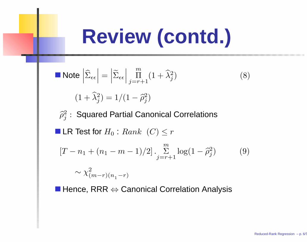
Note∣∣∣Σǫǫ
∣∣∣ =∣∣∣Σǫǫ
∣∣∣m
Πj=r+1
(1 + λ2j ) (8)
(1 + λ2j ) = 1/(1 − ρ2
j)
ρ2j : Squared Partial Canonical Correlations
LR Test for H0 : Rank (C) ≤ r
[T − n1 + (n1 − m − 1)/2] .m
Σj=r+1
log(1 − ρ2j) (9)
∼ χ2(m−r)(n
1−r)
Hence, RRR ⇔ Canonical Correlation Analysis
Reduced-Rank Regression – p. 6/??

VAR ModelsNumber of Parameters depend on order ‘p’ and dimension ‘m’
Stationarity imposes constraints on the AR Coefficient matrices
Anderson (2002) : Canon Corr / VAR RR
Box & Tiao (1977): Cannon Corr/Non-stationarity – Cointegrationideas
Reduced-Rank Regression – p. 7/??

VAR/RR - FeaturesYt = Φ1Yt−1 + Φ2Yt−2 + ǫt (10)
Φ2 – reduced-rank; Φ1 –Full rank – Anderson’s Model
Rank (Φ1: Φ2 ) lower rank;
Yt = A(B1 : B2)
Yt−1
Yt−2
+ ǫt (11)
(Velu et al 1986)
Yt = A1BYt−1 + A2BYt−2 + ǫt (12)
(Reinsel 1985) -Index Model
Let Φj = AjBj and range (Aj+1) ⊂ range (Aj)
(Ahn and Reinsel, 1988) –Nested RR
Reduced-Rank Regression – p. 8/??

VAR- Unit RootFeatures
Model (10) : Yt − Φ1Yt−1 − Φ2Yt−2 = Φ(L)Yt = ǫt
|Φ(L)| = 0,has d ≤ m unit roots; rest are outside unit circle
Error Correction (Granger) form:Wt = CYt−1 − Φ2Wt−1 + ǫt (13)
Rank (C)= Rank (- Φ (1)) ≤ r = m − d (14)
Thus, non-stationarity can be checked via reduced-rank test;Anderson (1951)
Implications of (14); Wt = Yt − Yt−1 is stationary
Reduced-Rank Regression – p. 9/??

VAR- Unit Root Features -Interpretation
Johansen (1988,1991)
Note (13) is: Wt = ABYt−1 − Φ2Wt−1 + ǫt...........(14)
BYt are stationary; rows of B are co-integrating vectors
Let Ztm×1
=
B
B∗
Yt, B∗ (d × m) is orthogonal to B
B∗Yt are non-stationary – “Common Trends”
Reduced-Rank Regression – p. 10/??

VAR-Unit Root-RRR -Advantages
Parsimonious Parametrization
Exhibit any “co-features” or “common features”
Improves forecasting
Other References are :
Tiao and Tsay (1988)
Hannan and Deistler (1988)
Engle and Kozicki (1993)
Min and Tsay (2005)
Reduced-Rank Regression – p. 11/??

Cointegration-UnitRoot-Tests
H0: Rank (C) = r vs H1 : Rank (C) < r
Johansen’s Trace Statistics:
Ltr(r) = −(T − mp)m
Σj=r+1
ln(1 − ρ2j) . . . ............(9)
Limiting distribution of Ltr is a standard Brownianmotion, depends only on ‘r’
Estimation of C,A,B etc. all follow from Anderson(1951)
Reduced-Rank Regression – p. 12/??

Beyond Cointegration –Common Features
Note that in ModelWt = ABYt−1 − Φ2Wt−1 + ǫt,
the component BYt−1is stationary
Find l′
i ∋ l′
iA = 0 spans the co-feature space(Anderson 1951)
Find l′
i ∋ l′
iA = 0 and l′
iΦ2 = 0 , Serial CorrelationCommon Feature (Engle & Kozicki 1993)
Common Seasonality (Hecq et al 2006)
Review Paper : Urga (2007)
Reduced-Rank Regression – p. 13/??

Numerical ExampleFour Quarterly Series : Private Investment, GNP, Consumptionand Unemployment,1951-1988,T= 148 ( See Figure 1)
VAR(2) is specified; also rank (Φ2) = 1 based on partial CanonicalCorrelations (See Table 2)
Recall that Partial Canonical analysis between Wt and Yt−1, givenWt−1 ⇔ LR for Unit Roots;
Results suggests d = 2 unit roots,thus r = 2 cointegrating ranks;(See Table 3)
Model (14) :Wt = CYt−1 − Φ2Wt−1 + ǫt
Reduced-Rank Regression – p. 14/??

Figure 1
Reduced-Rank Regression – p. 15/??

Table 2
Reduced-Rank Regression – p. 16/??

Table 3
Reduced-Rank Regression – p. 17/??

Numerical Example (contd.)
Estimation with ‘Cointegrating’ Reduced Rank Imposed
C=AB=
−0.241 0
−0.022 0
−.01 .107
−.209 −.921
1 0 −.997 .092
0 1 −.942 .094
=
−0.241 0 0.24 −.02 22
−0.022 0 .022 −.002
−0.01 0.107 −.09 .009
−0.209 −0.921 1. 07 −0.105
−Φ2 =
1
.167
.070
−1.673
[.239 0 2.724 0
]=
0.239 0 2. 724 0
.04 0 0.454 91 0
0.017 0 0.190 68 0
−0.400 0 −4. 557 3 0
∣∣∣Σǫ
∣∣∣ = 4.503 × 10⁻¹⁵ -Estimates ∼Full Rank LSES Reduced-Rank Regression – p. 18/??

Numerical Example (contd.)
Implications / Interpretation
Cointegration : Stationary Combinations:∗
Z3t = Y1t − 0.997Y3t + 0.042Y4t∗
Z4t = Y2t − 0.942Y3t + 0.094Y4t
Common Trend Components:∗
Z1t = b′
1Yt and∗
Z2t = b′
2Yt
where b′
1A and b′
2A = 0;
choose b1 ∋ b′
1Φ2 = b′
1a3d′ = 0
Thus, b′
1Wt = b′
1ξt, so∗
Z1t = b′
1Yt is a random walk∗
Z1t = −0.132Y1t + Y2t + 0.285Y3t + 0.033Y4t
See Figure 2Reduced-Rank Regression – p. 19/??

Figure 2
Reduced-Rank Regression – p. 20/??
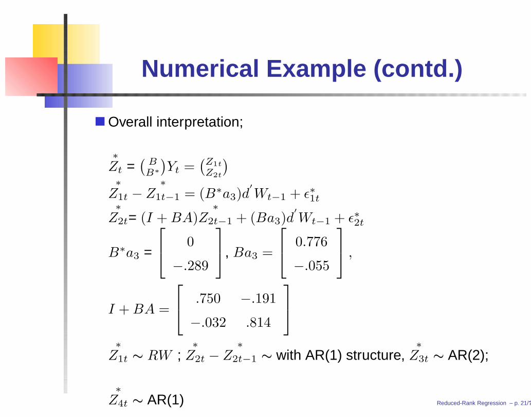
Numerical Example (contd.)
Overall interpretation;
∗
Zt =(
BB∗
)Yt =
(Z1t
Z2t
)
∗
Z1t −∗
Z1t−1 = (B∗a3)d′
Wt−1 + ǫ∗1t∗
Z2t= (I + BA)∗
Z2t−1 + (Ba3)d′
Wt−1 + ǫ∗2t
B∗a3 =
0
−.289
, Ba3 =
0.776
−.055
,
I + BA =
.750 −.191
−.032 .814
∗
Z1t ∼ RW ;∗
Z2t −∗
Z2t−1 ∼ with AR(1) structure,∗
Z3t ∼ AR(2);
∗
Z4t ∼ AR(1) Reduced-Rank Regression – p. 21/??

Forecasting-Applications
Effect of RR estimation on prediction, Rank (C) = 1; C = αβ′
Covariance matrix of the prediction error:
(1 + x′
0(XX′)−1
x0)Σǫǫ−{x
′
0(XX′
)−1x0 −(β
′
x0)2
β′ (XX′ )−1β
}(Σǫǫ−Σ1/2
ǫǫ V1V′
1Σ1/2ǫǫ )
( Reinsel and Velu, 1998, p46)
Empirical Analysis of Hog data indicate accounting for bothnon-stationarity and rank reduction consistently outperforms wellat all forecasting horizons ( Wang and Bessler 2004)
Reduced-Rank Regression – p. 22/??

RRR and Shrinkage
Recall C = AB = Σ1/2yy V
(r)∗ V
(r)′
∗ Σ−1/2yy C
= H−11 ∆1H1C
where ∆1 = Diag(1, 1, ......, 1, 0...0), m× m diagonal matrixGCV - Breiman and Friedman (1997)
Reinsel (1998)
∆1 = Diag(dj) , dj =(1−p1)(ρ
2
j−p1)
(1−p1)2ρ2
j+p2
1(1−ρ2
j)
j = 1 . . .m
where p1 = n1/(T − n2)
Reduced-Rank Regression – p. 23/??

ForecastingApplications -Contd.
Forecasting Large Datasets (Carriero, Kapetanoos & Marcellino 2007)
-RRR (Reinsel and Velu, 1998)-BVAR (Doan et al, 1984)
-BRR (Geweke, 1996)-RRP (Restrictions on the posterior mean)
-MB (Brieman, 1996)-FM (Stock and Watson 2002)
Data: 52 US Macroeconomic series (Real, Monetary &Financial)
Three Benchmarks: AR (1), BVAR and RW;
Among the six models: BRR -Short horizons
RRP -Long HorizonsFM- Best for 1-step ahead.
Conclusion: Using Shrinkage and Rank reduction in combinationReduced-Rank Regression – p. 24/??

Future WorkShrinkage -RRR, Needs further investigation
Yuan et al 2007-RRR/ LASSO
Impact of Rank Misspecification : Anderson(2002)
More broadly, in VAR context, the impact ofmisspecification of both the order ’p’ andrank ’r’ need to be studied.
Reduced-Rank Regression – p. 25/??