REDUCED FREQUENCY MOTOR STARTING FOR THIRD WORLD …

University of Kentucky University of Kentucky

UKnowledge UKnowledge

University of Kentucky Master's Theses Graduate School

2009

REDUCED FREQUENCY MOTOR STARTING FOR THIRD WORLD REDUCED FREQUENCY MOTOR STARTING FOR THIRD WORLD

POWER SYSTEMS POWER SYSTEMS

Taylor A. Begley University of Kentucky, [email protected]

Right click to open a feedback form in a new tab to let us know how this document benefits you. Right click to open a feedback form in a new tab to let us know how this document benefits you.

Recommended Citation Recommended Citation Begley, Taylor A., "REDUCED FREQUENCY MOTOR STARTING FOR THIRD WORLD POWER SYSTEMS" (2009). University of Kentucky Master's Theses. 607. https://uknowledge.uky.edu/gradschool_theses/607

This Thesis is brought to you for free and open access by the Graduate School at UKnowledge. It has been accepted for inclusion in University of Kentucky Master's Theses by an authorized administrator of UKnowledge. For more information, please contact [email protected].

http://uknowledge.uky.edu/

http://uknowledge.uky.edu/

https://uknowledge.uky.edu/

https://uknowledge.uky.edu/gradschool_theses

https://uknowledge.uky.edu/gradschool

https://uky.az1.qualtrics.com/jfe/form/SV_9mq8fx2GnONRfz7

mailto:[email protected]

ABSTRACT OF THESIS

REDUCED FREQUENCY MOTOR STARTING FOR THIRD WORLD POWER SYSTEMS

People in modern industrialized societies live a blessed life relative to those who do not when it comes to some modern conveniences. While many think nothing of flipping on a light switch or running electric appliances, there are people in third world countries could not imagine such things. As service projects are being undertaken to bring such conveniences to those less fortunate, there often is the harsh reality of a strict budget. An item that commands a large portion of said budget is often the diesel generator used to provide the facility with electricity. Generators serving motor loads are typically oversized due to a large kVA starting requirement. This paper addresses an approach to this problem by temporarily restricting the generator fuel supply by pulling back the rack of the mechanical governor reducing the frequency and voltage output as a motor load is switched onto the system. By reducing the voltage and frequency output of the generator, the motor is switched on at a time when its typically poor power factor and resulting kVA requirement is mitigated by the lower voltage and frequency allowing for a smaller generator to be used.

KEYWORDS: Reduced Frequency, Motor Starting, Third World Power, Reduced Voltage, Mechanical Governor

_______ Taylor A. Begley ________

________June 30, 2009__________


By

Taylor Andrew Begley

______Dr. Jimmie J. Cathey_______

Director of Thesis

_______Dr. Stephen Gedney______

Director of Graduate Studies

Date_________June 30, 2009_________

RULES FOR USE OF THESES

Unpublished theses submitted for the Master’s degree and deposited in the University of Kentucky Library are as a rule open for inspection, but are to be used only with due regard to the rights of the authors. Bibliographical references may be noted, but quotations or summaries of parts may be published only with the permission of the author, and with the usual scholarly acknowledgements.

Extensive copying or publication of the thesis in whole or in part also requires the consent of the Dean of the Graduate School of the University of Kentucky.

A library that borrows this thesis for use by its patrons is expected to secure the signature of each user.

Name Date ________________________________________________________________________

________________________________________________________________________

________________________________________________________________________

________________________________________________________________________

________________________________________________________________________

________________________________________________________________________

________________________________________________________________________

________________________________________________________________________

________________________________________________________________________

THESIS


The Graduate School

University of Kentucky

2009


________________________________

THESIS

________________________________

A thesis submitted in partial fulfillment of the

Requirements for the degree of Master of Science in Electrical Engineering

in the College of Engineering at the University of Kentucky

By


Lexington, Kentucky

Director: Dr. Jimmie J. Cathey, Professor of Electrical Engineering

Lexington, Kentucky

2009

Copyright © Taylor Andrew Begley 2009

iii

TABLE OF CONTENTS

LIST OF FIGURES .............................................................................................................................. iv

Chapter 1: Introduction .................................................................................................................. 1

Chapter 2: Presentation of the Problem ......................................................................................... 4

Chapter 3: Presentation of the Solution ......................................................................................... 8

The System Model ..................................................................................................................... 11

The Generator ........................................................................................................................ 12

The Induction Motor .............................................................................................................. 20

The Centrifugal Pump ............................................................................................................ 24

The Parallel Load .................................................................................................................... 28

Chapter 4: Presentation of the Results ......................................................................................... 29

Case I: 20 hp pump with a 45 kW parallel load.......................................................................... 29

Case II: 20 hp pump with a 10 kW parallel load......................................................................... 38

Case III: 20 hp pump only ........................................................................................................... 47

Critical Points ............................................................................................................................. 53

Generator Excitation Type ......................................................................................................... 61

Chapter 5: Conclusions ................................................................................................................. 67

Chapter 6: Recommendation for Future Work ............................................................................. 68

Appendices ..................................................................................................................................... 70

Appendix A: MATLAB Code ........................................................................................................ 70

Appendix B: Centrifugal Pump Data .......................................................................................... 81

References ..................................................................................................................................... 82

Vita ................................................................................................................................................. 83

iv

LIST OF FIGURES

Figure 1: Required Apparent Power for Startup with Different Parameters ................................... 9Figure 2: Flyball Governor .............................................................................................................. 10Figure 3: System Schematic ........................................................................................................... 12Figure 4: Sample Generator Waveform ......................................................................................... 14Figure 5: Approximate Generator Equivalent Circuit .................................................................... 16Figure 6: Voltage-Frequency Curve for a Separately Excited Generator ....................................... 18Figure 7: Voltage-Frequency Curve for a Self Excited Generator .................................................. 19Figure 8: Torque-Speed Curve for the Induction Motor ................................................................ 21Figure 9: Per Phase Induction Motor Equivalent Circuit ................................................................ 22Figure 10: Load Torque-Speed Curve for the Centrifugal Pump .................................................... 26Figure 11: Case I – Excitation and Terminal Voltages .................................................................... 30Figure 12: Case I - Current into the Motor ..................................................................................... 31Figure 13: Case I - Motor Shaft Speed ........................................................................................... 32Figure 14: Case I - Real Power into the Motor ............................................................................... 33Figure 15: Case I - Apparent Power into the Motor ...................................................................... 34Figure 16: Case I – 45 kW Parallel Load Real Power ...................................................................... 35Figure 17: Case I – 45 kW Parallel Load Apparent Power .............................................................. 35Figure 18: Case I – Total System Real Power ................................................................................. 36Figure 19: Case I – Total System Apparent Power ......................................................................... 37Figure 20: Case II – Excitation and Terminal Voltages ................................................................... 39Figure 21: Case II - Current into the Motor .................................................................................... 40Figure 22: Case II - Motor Shaft Speed .......................................................................................... 41Figure 23: Case II – Real Power into the Motor ............................................................................. 42Figure 24: Case II – Apparent Power into the Motor ..................................................................... 43Figure 25: Case II – 10 kW Parallel Load Real Power ..................................................................... 44Figure 26: Case II – 10 kW Parallel Load Apparent Power ............................................................. 44Figure 27: Case II – Total System Real Power ................................................................................ 45Figure 28: Case II – Total System Apparent Power ........................................................................ 46Figure 29: Case III – Excitation and Terminal Voltages .................................................................. 48Figure 30: Case III – Current into the Motor .................................................................................. 49Figure 31: Case III – Motor Shaft Speed ......................................................................................... 50Figure 32: Case III – Total System Real Power ............................................................................... 51Figure 33: Case III – Total System Apparent Power ....................................................................... 52Figure 34: Total System Power if there was No Transient Effects in the Motor ........................... 54Figure 35: Case I - Percent Improvement ...................................................................................... 56Figure 36: Case I – System Power with the Critical Point Utilized ................................................. 57Figure 37: Case II - Percent Improvement ..................................................................................... 59Figure 38: Case II – Total System Power with the Critical Point Utilized ....................................... 60

v

Figure 39: Self versus Separately Excited – Terminal Voltage ....................................................... 62Figure 40: Self versus Separately Excited – Current into the Motor ............................................. 63Figure 41: Self versus Separately Excited – Motor Shaft Speed .................................................... 64Figure 42: Self versus Separately Excited – Total System Real Power ........................................... 65Figure 43: Self versus Separately Excited – Total System Apparent Power ................................... 66

- 1 -

Chapter 1: Introduction

Our standards in life are often a product of our economic status. A man

accustomed to eating filet minion may scoff at the idea of eating a chopped sirloin.

Similarly, a man who has very little to eat would be more than happy with that same

sirloin. This situation is analogous to the problem that is presented in this paper. The

solution to the surveyed problem is one that could greatly improve the lives of people in

impoverished third world countries, but would be more than likely unacceptable to

those accustomed to the living standards in places like the USA.

The needs and problems encountered by those in third world countries seem to

be limitless. In this paper, I will describe a solution to a problem that would make life a

little better for those that are less fortunate. This issue is the availability of an affordable

means of obtaining water that is suitable for consumption. Unfortunately, the surface

water, including creeks, streams and lakes, in many third world countries are extremely

polluted from various sources. Not the least of these sources is sewage. As you can

image, the lack of sanitary drinking water plays a large role in the spread of disease in

these societies. There are other sources of water available that are far less dangerous.

Unfortunately, those sources may be 80 or 100 meters deep into the ground. Once it is

reached, there still is the issue of bringing the water to the surface, and preferably into a

water tower for distribution to the community.

A relevant issue to explore is the current infrastructure in these regions. As one

would expect, these poor countries often lack the funds to have the luxury of a reliable

- 2 -

power grid like we enjoy here in the U.S. The power that exists in many of these places

could be described as erratic at best. To many of us, this would prove to be immensely

frustrating to not be able to count on having a reliable power source. Natives of these

areas, however, are often simply thankful for any power that they have and are less

concerned with the fact that outages lasting hours, or even days or weeks at a time are

not uncommon.

Again, consider the challenge of providing the community with adequate,

relatively clean water from deep within the earth. Normally, while the power to the

community is flowing, the source can be treated as an infinite bus. There is no issue with

running all of the common electrical loads that exist in the community. In addition,

starting and operating an induction motor that will be powering a pump that will bring

the water from the depths to the community’s water tower is a trivial issue. However, a

problem arises when the power provided by an unreliable utility fails.

Because the local utilities cannot be counted on for reliable power, there exist

many service projects that involve providing these communities with backup diesel

generators to run their most vital loads. One of these loads would likely include power

to run a pump in order to provide the community with sanitary drinking water. This is

the part of the story where this paper enters the scene. As mentioned before, the depth

required to reach sanitary water is likely in vicinity of 80-100 meters and the pump will

have to be relatively large to provide the necessary head to push the water to the height

- 3 -

of a water tower located above the surface. It would not be uncommon for this vertical

distance to exceed 100m.

When these communities are working to upgrade their facilities with backup

power generation via a diesel generator, financial resources are at a premium. As you

can imagine, these communities have budgets that are very tight, so everything done in

the process must be done with the utmost cost efficiency in mind. Even a few hundred

dollars could be enough money to make or break many projects. In order to look at

where money can be saved in these situations, we must look at the “big ticket” items.

Obviously, the big ticket item in this situation is the generator itself and the cost for the

generator is directly proportional to its size. A higher power requirement results in a

higher cost. The purpose of this paper is to explore a way in which to reduce the

required generator size, thus reducing project cost, without the use of additional

equipment that would further raise the project cost or complicate the operation of the

system.

- 4 -

Chapter 2: Presentation of the Problem

To further refine the definition of this problem, more specificity is required. In

aggregate, the common electrical loads that are involved with lighting, receptacles, etc.

act in a somewhat linear fashion and will never require more power to run them than

what is required when run in rated steady state conditions. Simply put, there is nothing

difficult or interesting about the way a light bulb responds in different scenarios as far as

its power requirements. Motors, in particular larger motors such as the one used to

pump the water from the well to the tower, act in a very interesting way when exposed

to different electrical situations. They certainly have different requirements as various

voltages and frequencies are impressed upon them. The requirements of a motor when

running at rated conditions and the requirements for the same motor when that motor

is being brought up to rated speed vary greatly. The inrush current that is required when

starting an induction motor with full voltage applied typically is on the order of 4-5

times the rated operating current. More importantly, the kVA requirement of starting a

motor is also much greater than the steady state requirement. The spike in current, in

conjunction with the poor power factor at low motor speeds, results in this huge kVA

spike.

The kVA capacity of the generator powering the system is the limiting factor. The

ability to supply adequate real power (kW) is certainly a constraint, but the kVA

demanded by this system is even a more prominent issue as the motor is accelerated to

rated speed. At the low speeds that occur during startup, the motor will draw high

- 5 -

currents at a very poor power factor. When huge currents are drawn during a full line

voltage start of a motor, they are drawn at such a poor power factor that measuring the

kW required by the system does not reveal the entire picture. Because of the poor

power factor, the requirement of the motor is better represented and described by

looking at the kVA required. Any technique that could reduce the kVA spike or offset its

effects would allow the system generator to be sized smaller. By slowing down the

generator, causing a drop in voltage and frequency, the difficulties and limitations

presented by poor power factor are somewhat mitigated. Also, by sizing the generator

smaller, you reduce the use of fuel and allow the generator to run at a higher

percentage of its capacity, allowing it to be more efficient.

Consider a system that consists of a common load (lighting, receptacles, etc.)

that is 20 kW with a 0.85 power factor and an induction motor that is driving a 20 hp

water pump. In steady state, after the motor is up to speed, the system power

requirement is roughly 43 kVA. The problem is that during the startup of the motor, it

spikes the required kVA, bringing the apparent power requirement up to roughly 105

kVA. Because of the few seconds it takes to start the motor, the project must buy a

generator that is capable of providing 244% of the actual steady state load after the

motor is started. If generators cost $400/kVA, then you are spending an extra $24,800

on a generator that will only be run at full capacity for less than a few seconds per

motor start. For projects with a very limited budget, that $24,800 may be not available

and may be enough to kill the project.

- 6 -

The purpose of this paper is to show a solution to the above problem that is

appropriate for the environment in which it is used. The objective is to provide a more

cost effective use of the limited project budget. Secondly, the solution must be rugged

and simple to operate. Lots of delicate electronic controls and/or a complex manner in

which the solution is implemented would contradict its applicability. Brief disturbances

to the supplied power are not an issue in this situation since poor power quality is

commonplace.

A literature search has only identified one application that directly relates to the

principle utilized in this study [1]. In reference 1, an oil-field pump is supplied by a

dedicated generator where the advantage of reduced voltage and frequency are

implemented to reduce the size of the required generator. However, this reference does

not provide any information on the theoretical performance analysis, if such was done.

Otherwise, it appears that this problem is one that has not been studied, and

understandably so, since the resulting power quality normally would not be acceptable

in an application having loads connected in parallel with the pump.

There are currently other ways that the problem in this study is being addressed.

The method of using capacitor banks or series reactors or the use of solid state motor

starting would all be nice, but would result in extra equipment and extra costs.

On the other hand, the underlying principle of reduced voltage and frequency

start of an induction motor is a common occurrence when the well-known constant

Volts/Hertz inverter drives an induction motor. In a general sense, the concept

- 7 -

introduced in this thesis mimics the Volts/Hertz inverter without the associated cost of

the power electronic equipment.

- 8 -

Chapter 3: Presentation of the Solution

The beauty of the solution to the problem of interest in this paper is in its

simplicity. In order to save money and use a smaller generator, achieving the goals laid

out in the previous section, inherent features of the generator can be used. The primary

factor causing the generator to be sized larger than the required steady state load, is the

spike in current due to the starting of the motor. When starting a motor at full voltage

and frequency from the power source, it is common to experience significant spikes in

current and kVA demanded. In order to avert this problem, one can reduce the

frequency and the voltage output of the diesel generator.

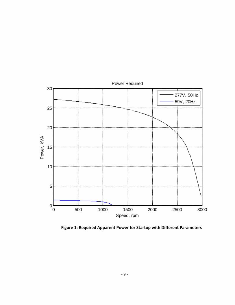
The Figure 1 shows the kVA requirements as a 22 hp motor and pump are

accelerated to rated speed. It is evident that the starting kVA requirement of a system

running at 59V and 20Hz (1.33kVA), which are the minimums set for the model

simulations, requires significantly less apparent power than the full line starting

parameters of 277V and 50Hz (27.20kVA). Below the aforementioned minimum starting

speed, the generator has difficulty providing the necessary power to supply the pump

with enough torque to begin its acceleration. The power produced at this lower

frequency, however, is adequate to begin the acceleration of the motor-pump. While

the time for the pump to accelerate to full speed is increased, this is a reasonable

tradeoff for the reduction in demanded power from the generator. This capability of

reducing the kVA requirement at the low speeds that exist during motor startup is the

crux upon which the entire solution is built.

- 9 -

Figure 1: Required Apparent Power for Startup with Different Parameters

0 500 1000 1500 2000 2500 30000

5

10

15

20

25

30Power Required

Speed, rpm

Pow

er, k

VA

277V, 50Hz59V, 20Hz

- 10 -

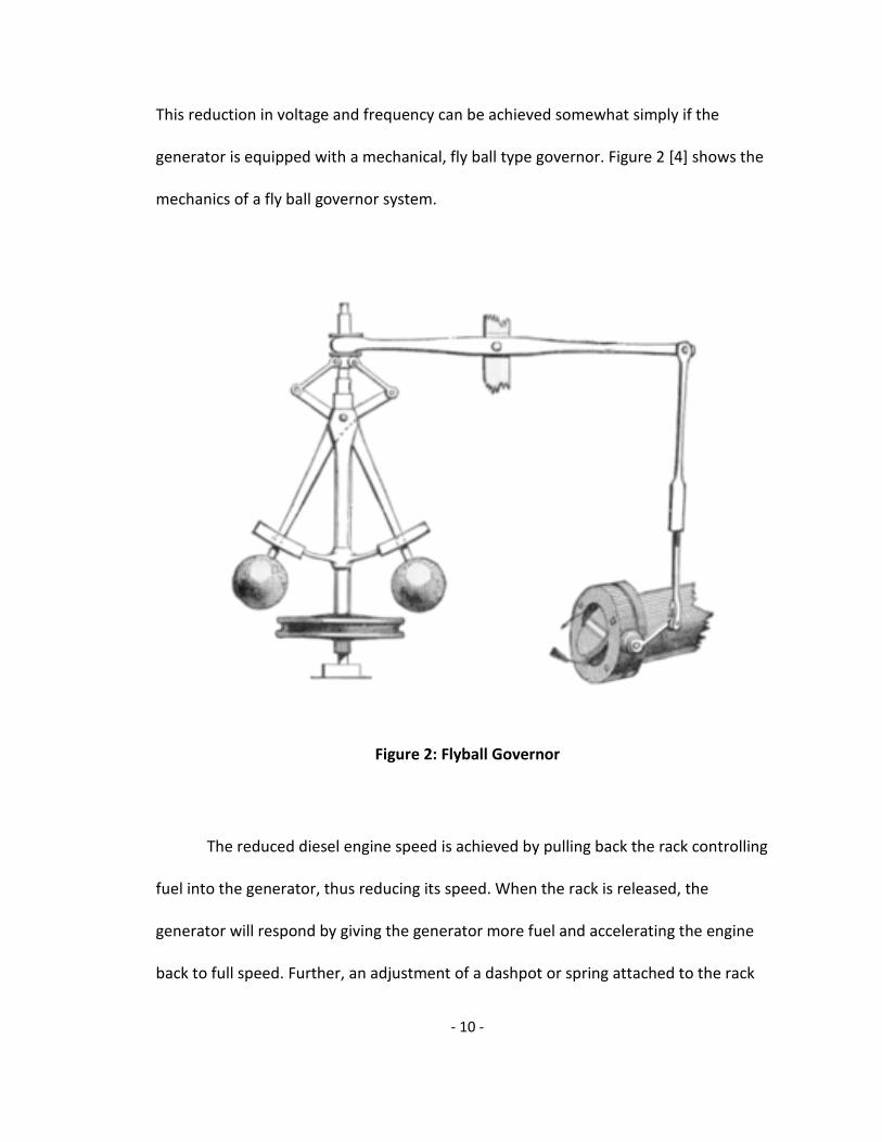
This reduction in voltage and frequency can be achieved somewhat simply if the

generator is equipped with a mechanical, fly ball type governor. Figure 2 [4] shows the

mechanics of a fly ball governor system.

Figure 2: Flyball Governor

The reduced diesel engine speed is achieved by pulling back the rack controlling

fuel into the generator, thus reducing its speed. When the rack is released, the

generator will respond by giving the generator more fuel and accelerating the engine

back to full speed. Further, an adjustment of a dashpot or spring attached to the rack

- 11 -

can be an easy, and indeed rugged, solution to adjusting the time desired to bring the

engine back up to full speed. Put simply, one person first pulls back the rack. Next, that

person (or another person) switches the induction motor on line and then the rack is

released. This allows the generator to accelerate back to full speed, eventually

providing the full rated voltage and frequency to the system. All of this occurs without

any adverse affects on the generator.

As seen in Figure 1, the lower voltage and frequency applied to the induction

motor allows the kVA requirement to be considerably lower than a full line start, while

still providing ample torque to bring the motor up to speed within a very reasonable

time frame. In fact, by the time the generator reaches full speed, the electrical

transients involved in getting the motor up to speed are complete. Because of this, the

large spike in electrical requirements can be partially, if not completely, offset before

the full rated voltage is regained and applied to the induction motor.

The System Model

In order to model this entire system, it was broken into several key components,

each of which can easily be modified to fit in the parameters of a given situation. A

simplified schematic of the model is shown in Figure 3 and a description of each

component follows. The model is tested and observed in the time frame required to

bring the entire system to steady state. For each increment of time tested, the model is

evaluated completely, the results are stored, and then the model moves to the next

iteration until the desired test time is elapsed. The model was designed and tested using

- 12 -

MATLAB. The code written to run the model and develop most of the plots in this

document can be found in the Appendix. The overall system that is about to be

described will serve a specific purpose. That purpose is to provide electrical service to a

system that includes common loads (receptacles, ceiling fans, etc.) as well as bringing

online an induction motor that is powering a pump that will provide a minimum of

120m of head to bring water from a deep well to a storage tower. The model that was

developed to simulate this system is remarkably versatile and can be, and will be,

tailored to evaluate the advantages of this system in a variety of different

circumstances.

The Generator

The action on the generator is the main mechanism in the system that is going to

allow this method to be successful. As discussed before, the rack of the generator will

Generator

Induction Motor

Centrifugal Pump

Parallel Load

Voltage, Frequency

Torque

Figure 3: System Schematic

- 13 -

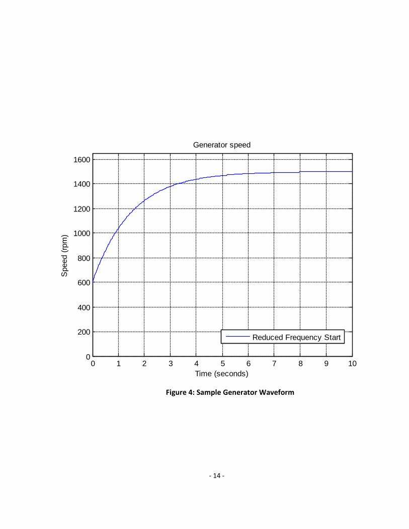
be pulled back, reducing the generator speed to a selected percentage of synchronous

speed. In the model, a 4 pole 50 Hz generator is used, which has synchronous speed of

1500 rpm. After the rack is released, the generator will accelerate back to the

synchronous speed in a given amount of time. This amount of time can easily be

adjusted in the model. In practice, it could be adjusted by altering the dashpot that

damps the rack movement back to its initial, full speed position. It is the assumption of

this simulation that it will accelerate to synchronous speed exponentially. For example:

if it is desired that the generator to be reduced to 40% speed and recover to full speed

in ten seconds, the generator output frequency would look like the speed-time curve of

Figure 4.

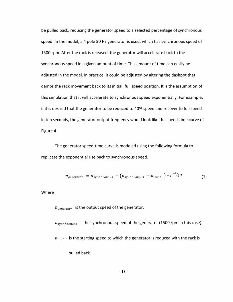
The generator speed-time curve is modeled using the following formula to

replicate the exponential rise back to synchronous speed.

𝑛𝑛𝑔𝑔𝑔𝑔𝑛𝑛𝑔𝑔𝑔𝑔𝑔𝑔𝑔𝑔𝑔𝑔𝑔𝑔 = 𝑛𝑛𝑠𝑠𝑠𝑠𝑛𝑛𝑠𝑠 ℎ𝑔𝑔𝑔𝑔𝑛𝑛𝑔𝑔𝑟𝑟𝑠𝑠 − �𝑛𝑛𝑠𝑠𝑠𝑠𝑛𝑛𝑠𝑠 ℎ𝑔𝑔𝑔𝑔𝑛𝑛𝑔𝑔𝑟𝑟𝑠𝑠 − 𝑛𝑛𝑖𝑖𝑛𝑛𝑖𝑖𝑔𝑔𝑖𝑖𝑔𝑔𝑖𝑖 � ∗ 𝑔𝑔−𝑔𝑔

1.7� (1)

Where

𝑛𝑛𝑔𝑔𝑔𝑔𝑛𝑛𝑔𝑔𝑔𝑔𝑔𝑔𝑔𝑔𝑔𝑔𝑔𝑔 is the output speed of the generator.

𝑛𝑛𝑠𝑠𝑠𝑠𝑛𝑛𝑠𝑠 ℎ𝑔𝑔𝑔𝑔𝑛𝑛𝑔𝑔𝑟𝑟𝑠𝑠 is the synchronous speed of the generator (1500 rpm in this case).

𝑛𝑛𝑖𝑖𝑛𝑛𝑖𝑖𝑔𝑔𝑖𝑖𝑔𝑔𝑖𝑖 is the starting speed to which the generator is reduced with the rack is

pulled back.

- 14 -

Figure 4: Sample Generator Waveform

0 1 2 3 4 5 6 7 8 9 100

200

400

600

800

1000

1200

1400

1600

Generator speed

Time (seconds)

Spe

ed (r

pm)

Reduced Frequency Start

- 15 -

1.7 is an arbitrary time constant that determines the length of time for the

system to return to full speed.

Every generator will have its own voltage-frequency characteristic. However, the vast

majority will fall in one of two categories depending on the type of excitation involved. If

the generator is separately excited by a shaft mounted auxiliary generator, it will have a

characteristic curve that is quadratic in shape until reaching a pull-up voltage that brings

the output up to the fully rated voltage. This occurs due to the ability of the generator’s

exciter to temporarily provide the extra voltage to push the output voltage up the rated

voltage. It is not uncommon for the exciter to be able to compensate for a 15%-20% dip

in voltage. In the simulations for this paper, the voltage is pulled up to its full line level

at 85% of full frequency. Another key element to this analysis is the internal impedance

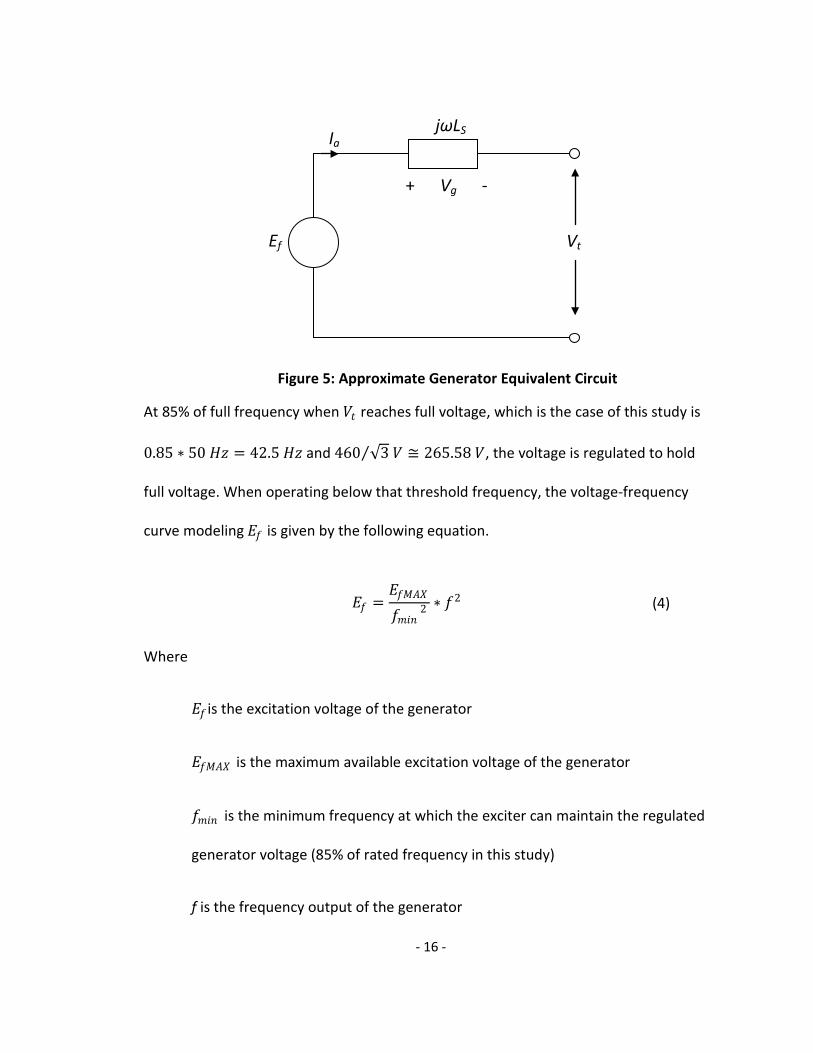
within the generator. The generator approximate equivalent circuit is shown in Figure 5.

Due to the generator internal impedance shown in the figure, the terminal 𝑉𝑉𝑔𝑔 , is not

directly proportional to the excitation voltage 𝐸𝐸𝑓𝑓 . On the contrary, 𝑉𝑉𝑔𝑔 , which is the

voltage seen by the induction motor and the parallel load, will be characterized by the

following equations:

𝑉𝑉𝑔𝑔 = 𝐸𝐸𝑓𝑓 − 𝑉𝑉𝑔𝑔 (2)

𝑉𝑉𝑔𝑔 = 𝐸𝐸𝑓𝑓 − 𝑗𝑗𝑗𝑗𝐿𝐿𝑆𝑆(𝐼𝐼𝑔𝑔) (3)

- 16 -

At 85% of full frequency when 𝑉𝑉𝑔𝑔 reaches full voltage, which is the case of this study is

0.85 ∗ 50 𝐻𝐻𝐻𝐻 = 42.5 𝐻𝐻𝐻𝐻 and 460 √3 𝑉𝑉 ≅ 265.58 𝑉𝑉⁄ , the voltage is regulated to hold

full voltage. When operating below that threshold frequency, the voltage-frequency

curve modeling 𝐸𝐸𝑓𝑓 is given by the following equation.

𝐸𝐸𝑓𝑓 =𝐸𝐸𝑓𝑓𝑓𝑓𝑓𝑓𝑓𝑓𝑓𝑓𝑚𝑚𝑖𝑖𝑛𝑛

2 ∗ 𝑓𝑓2 (4)

Where

𝐸𝐸𝑓𝑓 is the excitation voltage of the generator

𝐸𝐸𝑓𝑓𝑓𝑓𝑓𝑓𝑓𝑓 is the maximum available excitation voltage of the generator

𝑓𝑓𝑚𝑚𝑖𝑖𝑛𝑛 is the minimum frequency at which the exciter can maintain the regulated

generator voltage (85% of rated frequency in this study)

f is the frequency output of the generator

Vt

jωLS

Ef

Ia

+ Vg -

Figure 5: Approximate Generator Equivalent Circuit

- 17 -

This curve is shown in Figure 6.

If the generator is excited by its own rectified output, a frequency sensitive

excitation control can be designed to render a voltage-frequency curve that is linear

below a selected frequency. Regulated voltage is maintained above that frequency. The

curve in this region is modeled by the following formula and is shown in Figure 7.

𝐸𝐸𝑓𝑓 =𝐸𝐸𝑓𝑓𝑓𝑓𝑓𝑓𝑓𝑓𝑓𝑓𝑚𝑚𝑖𝑖𝑛𝑛

∗ 𝑓𝑓 (5)

Because the shaft speed of the motor is not constant, it is very difficult to analytically

predict the impedance of the motor at a given time. This further makes it difficult to find

the system current and the voltage drop across 𝑗𝑗𝑗𝑗𝐿𝐿𝑆𝑆 which would allow 𝐸𝐸𝑓𝑓 to be

calculated. In order to find 𝐸𝐸𝑓𝑓𝑓𝑓𝑓𝑓𝑓𝑓 , a trial and error method was used until the resulting

terminal voltage 𝑉𝑉𝑔𝑔was found to be piecewise continuous. The model in this study will

primarily be using the self excited generator, but the differences in the performance of

the system using the two different methods of excitation will be evaluated in Chapter 4.

- 18 -

Figure 6: Voltage-Frequency Curve for a Separately Excited Generator

20 25 30 35 40100

150

200

250

300

350

400

450

500

550Separately Excited Generator Characteristic Curve

Frequency (Hz)

Exc

itatio

n V

olta

ge (p

er p

hase

)

- 19 -

Figure 7: Voltage-Frequency Curve for a Self Excited Generator

20 25 30 35 40200

250

300

350

400

450

500

550Self Excited Generator Characteristic Curve

Frequency (Hz)

Exc

itatio

n V

olta

ge (p

er p

hase

)

- 20 -

The Induction Motor

Accurately modeling the induction model is an integral part of getting a useful

and valid result. The requirements of the induction motor are based solely on the power

requirement of the centrifugal pump that is to be discussed momentarily. The pump

that is selected for this simulation requires approximately 20 hp at the operating point,

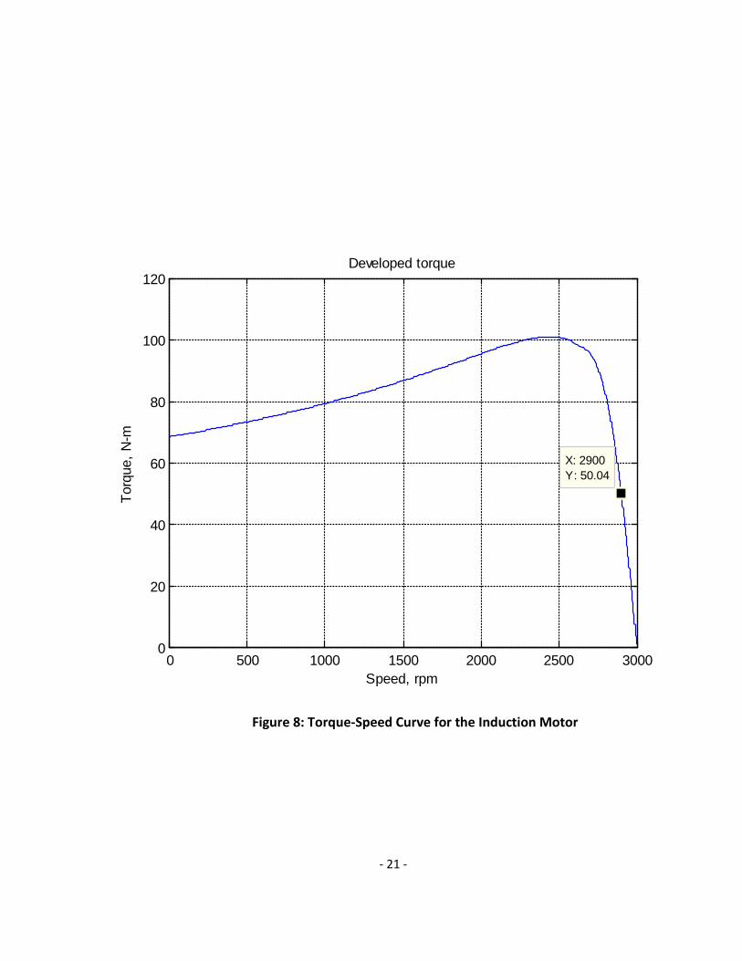
which is at 2900 rpm. Based upon typical induction motor efficiencies, the induction

motor will need to be a roughly 22 hp 2-pole motor. In order to accurately model this

motor, the induction motor parameters were selected accordingly to yield the torque-

speed curve of the motor as shown in Figure 8, ensuring that the motor operates at the

desired power output at the operating point of 2900 rpm. The above mentioned

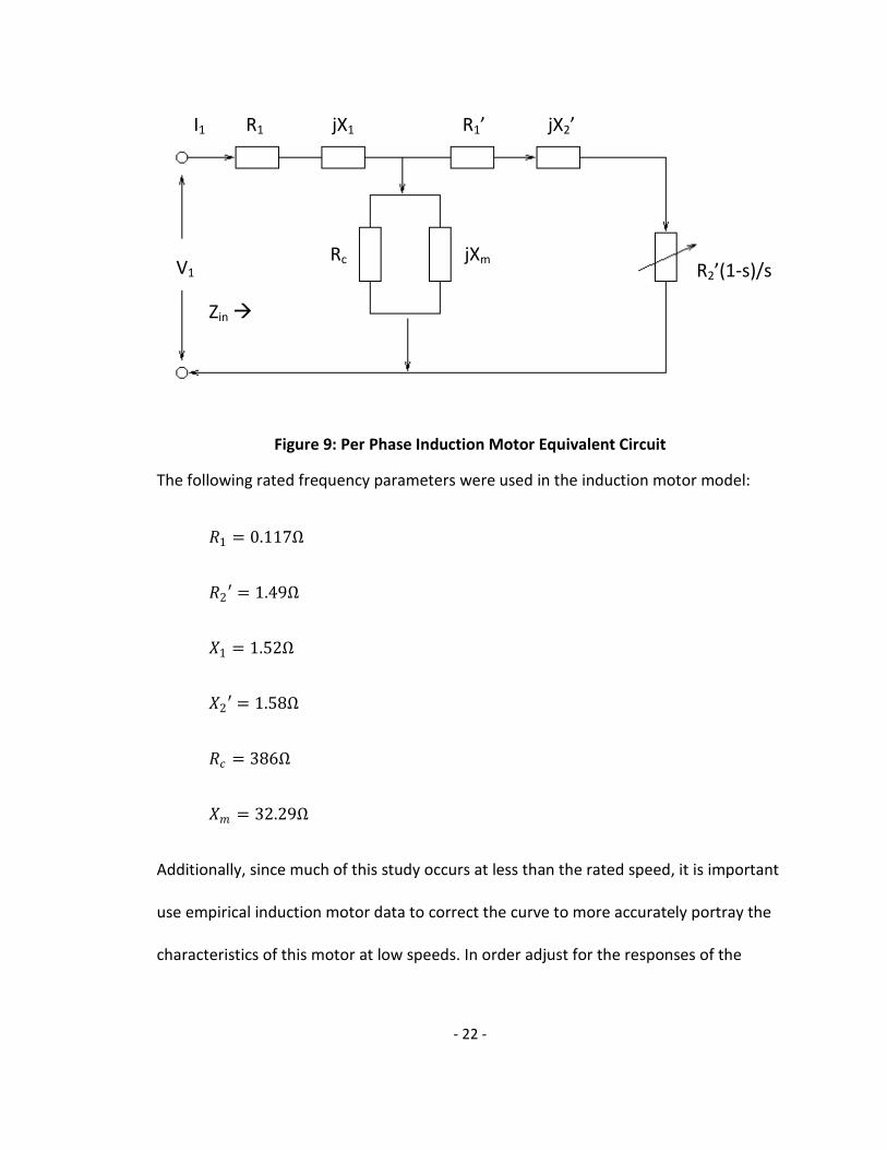
parameters that were selected were based upon the common induction motor per-

phase equivalent circuit as shown in Figure 9. Although the problem to be solved is not a

steady state case, the mechanical time constants are significantly greater than the

electrical time constants, thus sinusoidal steady state modeling of the induction motor is

justified.

- 21 -

0 500 1000 1500 2000 2500 30000

20

40

60

80

100

120

X: 2900Y: 50.04

Developed torque

Speed, rpm

Torq

ue, N

-m

Figure 8: Torque-Speed Curve for the Induction Motor

- 22 -

Figure 9: Per Phase Induction Motor Equivalent Circuit

The following rated frequency parameters were used in the induction motor model:

𝑅𝑅1 = 0.117Ω

𝑅𝑅2′ = 1.49Ω

𝑓𝑓1 = 1.52Ω

𝑓𝑓2′ = 1.58Ω

𝑅𝑅𝑠𝑠 = 386Ω

𝑓𝑓𝑚𝑚 = 32.29Ω

Additionally, since much of this study occurs at less than the rated speed, it is important

use empirical induction motor data to correct the curve to more accurately portray the

characteristics of this motor at low speeds. In order adjust for the responses of the

V1 R2’(1-s)/s Rc jXm

jX2’ R1’ jX1 R1 I1

Zin

- 23 -

resistance and leakage inductance at lower frequencies, a heuristic approach [2] is

incorporated into the model that accounts for the skin (or deep bar) effects.

During the operation of induction motors, there are unavoidable losses in power

attributed to friction and windage (𝑃𝑃𝐹𝐹&𝑊𝑊). In this simulation, the friction and windage

losses of the induction motor is set to 700W, which falls within the typical range of 3-5%

of the total power consumed by the motor. Once that number was determined, the

amount of torque due to friction and windage (𝑇𝑇𝐹𝐹&𝑊𝑊) can be calculated using the

following formula.

𝑇𝑇𝐹𝐹&𝑊𝑊 =𝑃𝑃𝐹𝐹&𝑊𝑊

𝜋𝜋30 ∗ 2900

(6)

Where

2900 is the steady state operating speed in revolutions per minute and

s is slip and is defined as

𝑠𝑠 =𝑛𝑛𝑠𝑠𝑠𝑠𝑛𝑛𝑠𝑠 ℎ𝑔𝑔𝑔𝑔𝑛𝑛𝑔𝑔𝑟𝑟𝑠𝑠 − 𝑛𝑛𝑚𝑚𝑔𝑔𝑔𝑔𝑔𝑔𝑔𝑔

𝑛𝑛𝑠𝑠𝑠𝑠𝑛𝑛𝑠𝑠 ℎ𝑔𝑔𝑔𝑔𝑛𝑛𝑔𝑔𝑟𝑟𝑠𝑠 (7)

Using the circuit in Figure 9, the following formulae can be applied to give several

meaningful results including current into the motor (𝐼𝐼1), power factor of the motor

(𝑃𝑃𝐹𝐹), real power into the motor �𝑃𝑃𝑖𝑖𝑛𝑛 ,𝑚𝑚𝑔𝑔𝑔𝑔𝑔𝑔𝑔𝑔 �, apparent power into the motor

�𝑆𝑆𝑖𝑖𝑛𝑛 ,𝑚𝑚𝑔𝑔𝑔𝑔𝑔𝑔𝑔𝑔 �, total developed torque (𝑇𝑇𝐷𝐷), and the torque output from the motor (𝑇𝑇𝑔𝑔𝑟𝑟𝑔𝑔 ).

- 24 -

𝐼𝐼1 =𝑉𝑉1

𝑍𝑍𝑖𝑖𝑛𝑛 (8)

𝑃𝑃𝐹𝐹 = cos�𝑔𝑔𝑛𝑛𝑔𝑔𝑖𝑖𝑔𝑔(𝑉𝑉1) − 𝑔𝑔𝑛𝑛𝑔𝑔𝑖𝑖𝑔𝑔(𝐼𝐼1)� (9)

𝑃𝑃𝑖𝑖𝑛𝑛 ,𝑚𝑚𝑔𝑔𝑔𝑔𝑔𝑔𝑔𝑔 = 3 ∗ 𝑉𝑉1 ∗ 𝐼𝐼1 ∗ 𝑃𝑃𝐹𝐹 (10)

𝑆𝑆𝑖𝑖𝑛𝑛 ,𝑚𝑚𝑔𝑔𝑔𝑔𝑔𝑔𝑔𝑔 =𝑃𝑃𝑖𝑖𝑛𝑛 ,𝑚𝑚𝑔𝑔𝑔𝑔𝑔𝑔𝑔𝑔

𝑃𝑃𝐹𝐹 (11)

𝑇𝑇𝐷𝐷 =3 ∗ 𝑝𝑝𝑔𝑔𝑖𝑖𝑔𝑔𝑠𝑠 ∗ (𝐼𝐼2′)2 ∗ 𝑅𝑅2

′

4 ∗ 𝜋𝜋 ∗ 𝑠𝑠 ∗ 𝑓𝑓 (12)

𝑇𝑇𝑔𝑔𝑟𝑟𝑔𝑔 = 𝑇𝑇𝐷𝐷 − 𝑇𝑇𝐹𝐹&𝑊𝑊 (13)

The input parameters for the induction motor part of the model are the voltage

and frequency output by the generator, as well as the current shaft speed of the motor.

Using these inputs, the model is able to compute the current that is drawn by the

motor, the total real and apparent power required by the motor, as well as the total

developed torque of the motor that is output to the centrifugal pump.

The Centrifugal Pump

The first step in modeling the centrifugal pump is to find appropriate parameters

from which we can accurately model its performance. The primary requirement of this

pump is that it must produce a minimum of 120 meters of head. This is assuming the

situation discussed involves pumping water from 80 meters below the surface to a

water tower that stands 40 meters tall. You will find the pump upon which the model is

based in the Appendix. The pump in this model is given a load torque requirement that

is typical for a centrifugal pump [3]. The shape of the curve is parabolic in nature and

- 25 -

begins with a torque requirement of 15% of the full load torque. From there, it

decreases to 10% of the full load torque at 20% of the rated full speed and then

increases proportional to speed squared until reaching its operating point. The speed

torque curve for the centrifugal pump is shown in Figure 10. As is evident by the curve,

the pump has an initial torque requirement at 6.3 Nm. From there, it decreases to 4.2

Nm at 580 rpm before growing quadratically toward the operating point of 2900 rpm

where the load is 42 Nm.

The input parameters for the pump part of the model are the total developed

torque and the shaft speed of the motor. In each iteration of the model, it ascertains

that the load torque of the pump is met or exceeded by the total developed torque

supplied by the induction motor.

The next step is calculating the change in speed that is accounted for by the

difference in the load torque of the pump and the developed torque that is supplied to

the pump. The difference results in an accelerating torque, which drives the system to

run at a higher speed. Computing the change in speed 𝑑𝑑𝑗𝑗𝑚𝑚𝑑𝑑𝑔𝑔

is achieved by solving the

following differential equation:

𝑇𝑇𝐷𝐷 = 𝐽𝐽𝑑𝑑𝑗𝑗𝑚𝑚𝑑𝑑𝑔𝑔

+ 𝑇𝑇𝐿𝐿 + 𝛽𝛽𝑗𝑗𝑚𝑚 (14)

where 𝑇𝑇𝐷𝐷,𝑇𝑇𝐿𝐿,and 𝑗𝑗𝑚𝑚 are given from earlier parts of the simulation. The last term, 𝛽𝛽𝑗𝑗𝑚𝑚 ,

is the losses due to friction and windage within the pump and motor. The moment of

inertia can be calculated using the following empirical formula [4] that

- 26 -

0 500 1000 1500 2000 2500 30000

5

10

15

20

25

30

35

40

45

50X: 2900Y: 42

Centrifugal Pump Torque-Speed Curve

Pump Speed (rpm)

Load

Tor

que

(Nm

)

Figure 10: Load Torque-Speed Curve for the Centrifugal Pump

- 27 -

determines the moments of inertia individually for the pump and the induction motor,

and then combines them to form the moment of inertia for the system.

𝐽𝐽𝑝𝑝𝑟𝑟𝑚𝑚𝑝𝑝 = 0.03768 �𝑃𝑃𝑁𝑁�

0.9556

(15)

𝐽𝐽𝑚𝑚𝑔𝑔𝑔𝑔𝑔𝑔𝑔𝑔 = 0.0043 �𝑃𝑃𝑁𝑁�

1.48

(16)

𝐽𝐽 = 𝐽𝐽𝑝𝑝𝑟𝑟𝑚𝑚𝑝𝑝 + 𝐽𝐽𝑚𝑚𝑔𝑔𝑔𝑔𝑔𝑔𝑔𝑔 (17)

Where

P is the mechanical power in kW

N is the pump speed in thousands of rpm

For the case being studied in this paper, the resulting moment of inertia for the motor-

pump combination is

𝐽𝐽 = 0.1547𝑘𝑘𝑔𝑔 ∙ 𝑚𝑚2

As the developed torque (𝑇𝑇𝐷𝐷) exceeds the load torque(𝑇𝑇𝐿𝐿), there will be an acceleration

of the pump. The increase in speed will occur until equilibrium is reached between the

load torque and the total developed torque, which implies that the accelerating torque

is zero and the stable operating point of the system has been reached. In this setup of

the system, that equilibrium is achieved at approximately 2900 rpm. The output of the

- 28 -

centrifugal pump portion of the model is the new shaft speed, which is based upon the

solved differential equation in equation (12). This result is used in the following iteration

of the model.

The Parallel Load

A critical variable in this problem that is being explored is the load on the system

that does not stem from the motor-pump. This proportion of the system power will be

dedicated to running common loads such as receptacles and ceiling fans in parallel with

the motor and will have a direct correlation with the usefulness of this technique. As the

motor load becomes a larger part of the overall system, the advantage of the proposed

technique will become more evident. In the model, the parallel load will be set to

various levels to provide analysis for the broad applicability of the technique. For the

setup in this paper, the power factor of the parallel load is 0.85, but this can easily be

changed to fit a specific situation.

All of the above modules are run, one increment at a time, for the duration of

the desired time span to be tested. Obviously, the time period that is interesting in this

situation is the time that it takes for the generator and the motor-pump combination to

reach their stable operating points. The model is one that will be used to test a variety

of different setups to explore and define the situations in which the technique is the

most relevant and useful.

- 29 -

Chapter 4: Presentation of the Results

Several different configurations were simulated using the model outlined in the

previous section. There are three primary setups that will be analyzed in this study. The

first two are those that power a 20 hp pump with parallel loads of 45 kW and 10 kW,

both with a 0.85 power factor. The third setup will only power the motor load. Cases I

and II represent systems where the steady state load of the pump motor is roughly 25%

and 60% of the total system steady state load, respectively, with the rack pulled back to

the point that allows the system to begin with the generator at 40% of synchronous

speed. Following those tests, further results from a broad range of situations will be

explored to draw a more generalized and robustly applicable result.

Case I: 20 hp pump with a 45 kW parallel load

From the system simulation, there are several results of interest. The purpose of

this paper is to illustrate the improvement of this technique against a full voltage and

frequency start of the system. Where applicable, the plot of the system using the novel

technique discussed here as well as the system without use of the technique will be

superimposed on the same axes in order to show the overall improvement in system

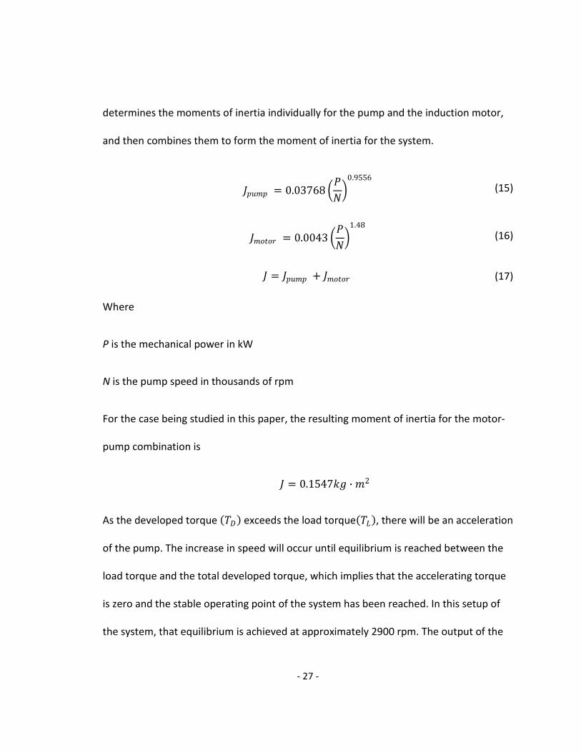
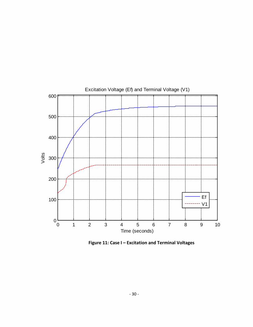
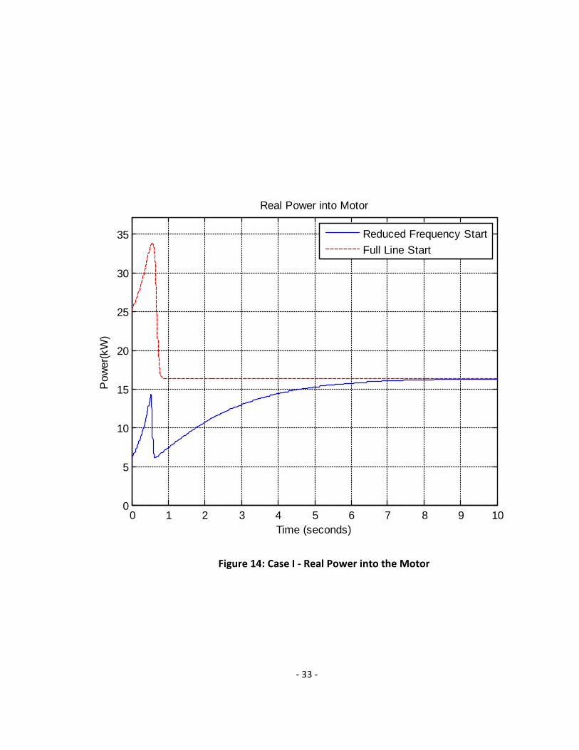
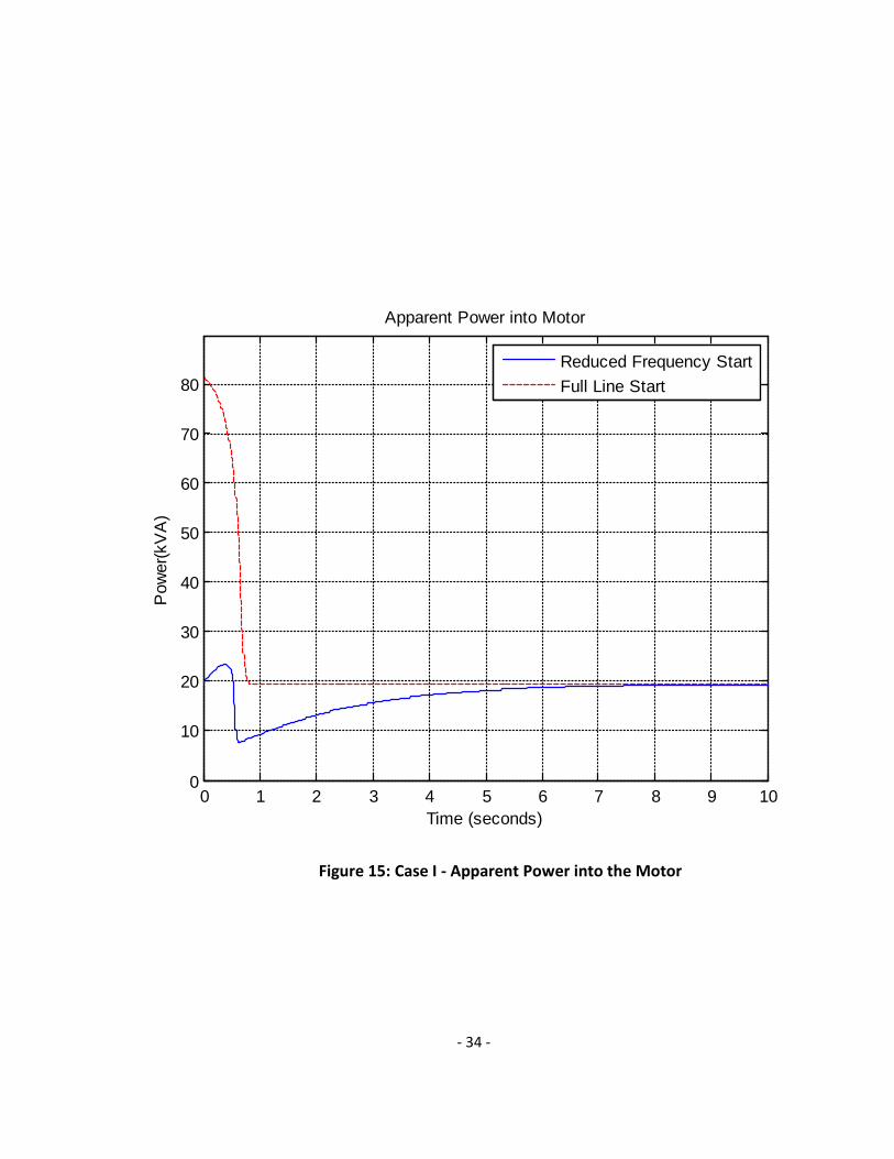
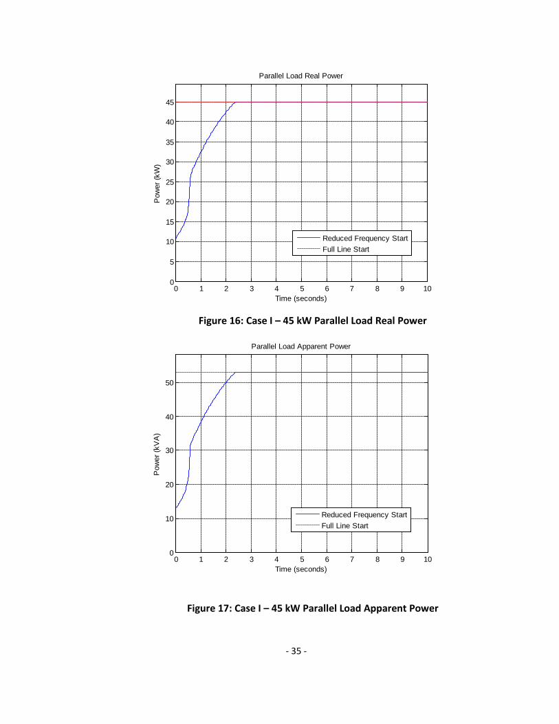
performance. Figures 11-17 show the excitation and terminal voltages, motor current ,

motor speed, parallel load average and apparent power requirements, motor average

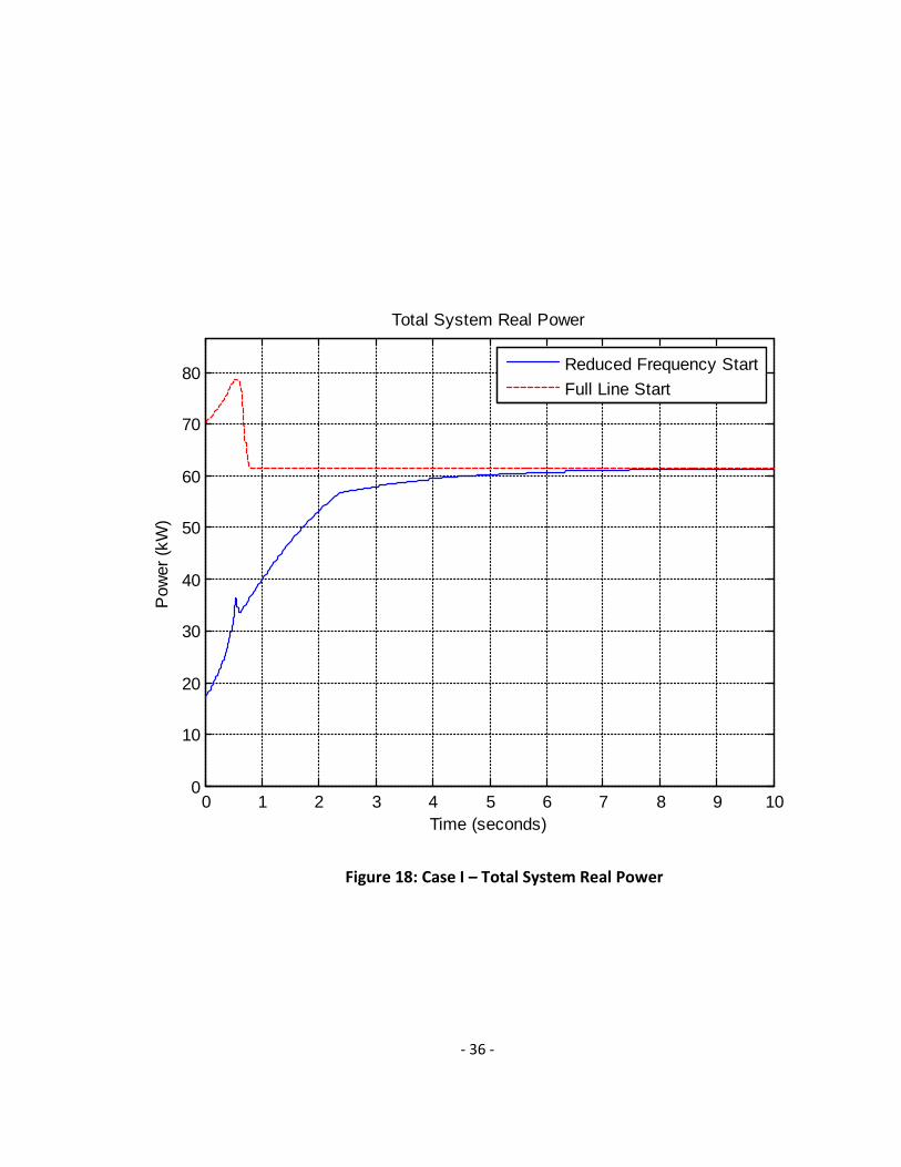
power input and motor apparent power input, respectively, for Case I. Figures 18 and 19

display, respectively the total average and apparent power required by both the motor

and the 45 kW parallel load.

- 30 -

Figure 11: Case I – Excitation and Terminal Voltages

0 1 2 3 4 5 6 7 8 9 100

100

200

300

400

500

600Excitation Voltage (Ef) and Terminal Voltage (V1)

Time (seconds)

Vol

ts

EfV1

- 31 -

Figure 12: Case I - Current into the Motor

0 1 2 3 4 5 6 7 8 9 100

20

40

60

80

100

Motor Current

Time (seconds)

Cur

rent

(per

pha

se)

Reduced Frequency StartFull Line Start

- 32 -

Figure 13: Case I - Motor Shaft Speed

0 1 2 3 4 5 6 7 8 9 100

500

1000

1500

2000

2500

3000

Motor Shaft Speed

Time (seconds)

Spe

ed(n

m)


- 33 -

Figure 14: Case I - Real Power into the Motor

0 1 2 3 4 5 6 7 8 9 100

5

10

15

20

25

30

35

Real Power into Motor

Time (seconds)

Pow

er(k

W)


- 34 -

Figure 15: Case I - Apparent Power into the Motor

0 1 2 3 4 5 6 7 8 9 100

10

20

30

40

50

60

70

80

Apparent Power into Motor

Time (seconds)

Pow

er(k

VA

)


- 35 -

Figure 16: Case I – 45 kW Parallel Load Real Power

Figure 17: Case I – 45 kW Parallel Load Apparent Power

0 1 2 3 4 5 6 7 8 9 100

10

20

30

40

50

Parallel Load Apparent Power

Time (seconds)

Pow

er (k

VA

)


0 1 2 3 4 5 6 7 8 9 100

5

10

15

20

25

30

35

40

45

Parallel Load Real Power

Time (seconds)

Pow

er (k

W)


- 36 -

Figure 18: Case I – Total System Real Power

0 1 2 3 4 5 6 7 8 9 100

10

20

30

40

50

60

70

80

Total System Real Power

Time (seconds)

Pow

er (k

W)


- 37 -

Figure 19: Case I – Total System Apparent Power

0 1 2 3 4 5 6 7 8 9 100

20

40

60

80

100

120

140

Total System Apparent Power

Time (seconds)

Pow

er (k

VA

)


- 38 -

The plot of most significance in this simulation is presented in Figure 19 which

shows the total system apparent power demanded by the combination of the motor

load as well as the 45 kW parallel load at 0.85 power factor. As is evident from the plot,

there are significant savings in the power requirement of the system when use the

technique outlined in this paper. More specifically, with a full line start, the maximum

apparent power requirement of the system peaks at 134.54 kVA. When using the

reduced frequency technique, the maximum apparent power requirement is 72.39 kVA.

In this case, the required apparent power supplied is reduced by 62.15 kVA, or 46%.

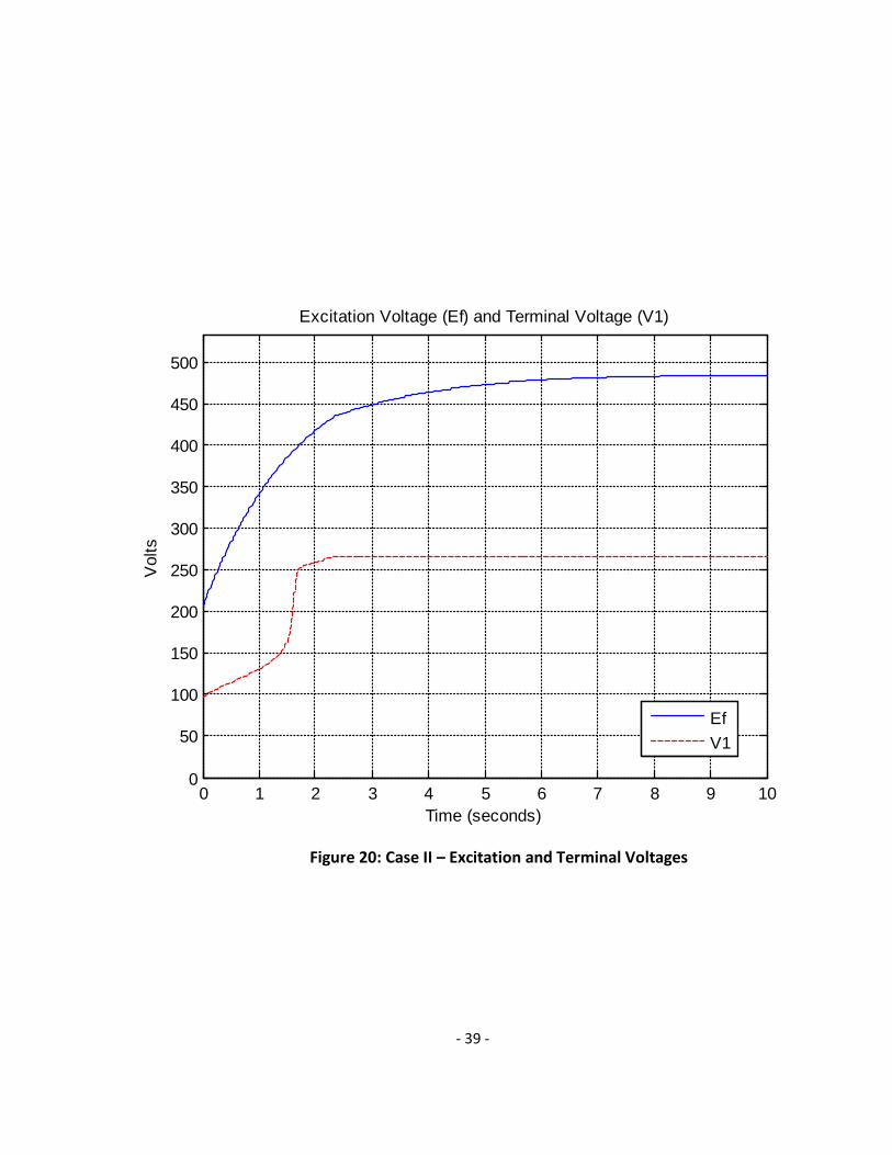
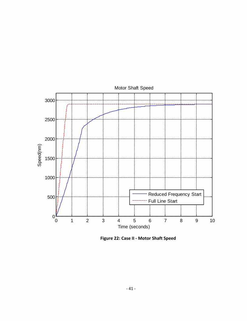
Case II: 20 hp pump with a 10 kW parallel load

The same logic and parameters were used when examining the case where the

parallel load was 10 kW with 0.85 power factor. Figures 20-26 show the excitation and

terminal voltages, motor current , motor speed, parallel load average and apparent

power requirements, motor average power input and motor apparent power input,

respectively, for Case I. Figures 27 and 28 display, respectively the total average and

apparent power required by both the motor and the 10 kW parallel load with Figure 28

being the plot of most significance in this simulation. There are significant savings in the

power requirement of the system when use the technique outlined in this paper. More

specifically, with a full line start, the maximum apparent power requirement of the

system peaks at 93.37 kVA. When using the reduced frequency technique, the

maximum apparent power requirement is 38.45 kVA. In this case, the required apparent

power supplied is reduced 59%.

- 39 -

Figure 20: Case II – Excitation and Terminal Voltages

0 1 2 3 4 5 6 7 8 9 100

50

100

150

200

250

300

350

400

450

500

Excitation Voltage (Ef) and Terminal Voltage (V1)

Time (seconds)

Vol

ts

EfV1

- 40 -

Figure 21: Case II - Current into the Motor

0 1 2 3 4 5 6 7 8 9 100

20

40

60

80

100

Motor Current

Time (seconds)

Cur

rent

(per

pha

se)


- 41 -

Figure 22: Case II - Motor Shaft Speed

0 1 2 3 4 5 6 7 8 9 100

500

1000

1500

2000

2500

3000

Motor Shaft Speed

Time (seconds)

Spe

ed(n

m)


- 42 -

Figure 23: Case II – Real Power into the Motor

0 1 2 3 4 5 6 7 8 9 100

5

10

15

20

25

30

35

Real Power into Motor

Time (seconds)

Pow

er(k

W)


- 43 -

Figure 24: Case II – Apparent Power into the Motor

0 1 2 3 4 5 6 7 8 9 100

10

20

30

40

50

60

70

80

Apparent Power into Motor

Time (seconds)

Pow

er(k

VA

)


- 44 -

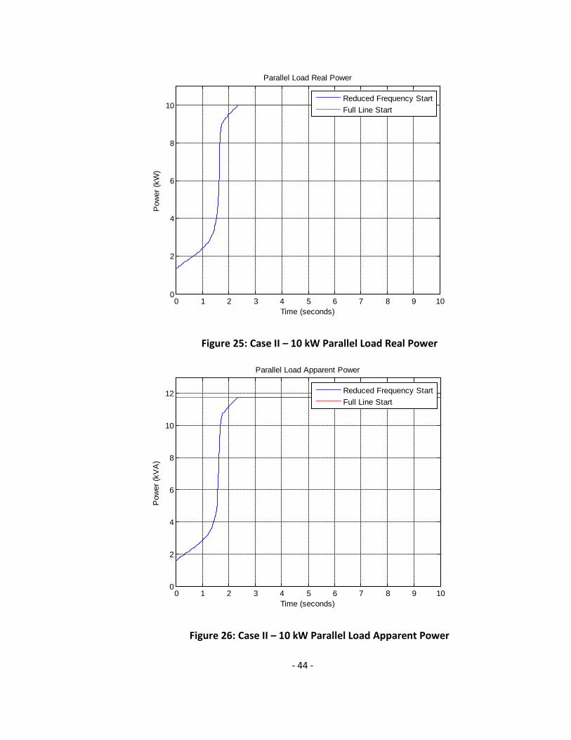
Figure 25: Case II – 10 kW Parallel Load Real Power

Figure 26: Case II – 10 kW Parallel Load Apparent Power

0 1 2 3 4 5 6 7 8 9 100

2

4

6

8

10

Parallel Load Real Power

Time (seconds)

Pow

er (k

W)


0 1 2 3 4 5 6 7 8 9 100

2

4

6

8

10

12

Parallel Load Apparent Power

Time (seconds)

Pow

er (k

VA

)


- 45 -

Figure 27: Case II – Total System Real Power

0 1 2 3 4 5 6 7 8 9 100

5

10

15

20

25

30

35

40

45


Time (seconds)

Pow

er (k

W)


- 46 -

Figure 28: Case II – Total System Apparent Power

0 1 2 3 4 5 6 7 8 9 100

10

20

30

40

50

60

70

80

90

100


Time (seconds)

Pow

er (k

VA

)


- 47 -

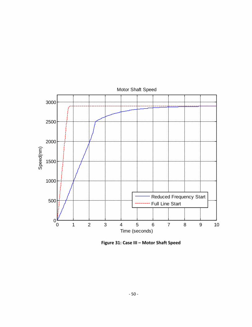
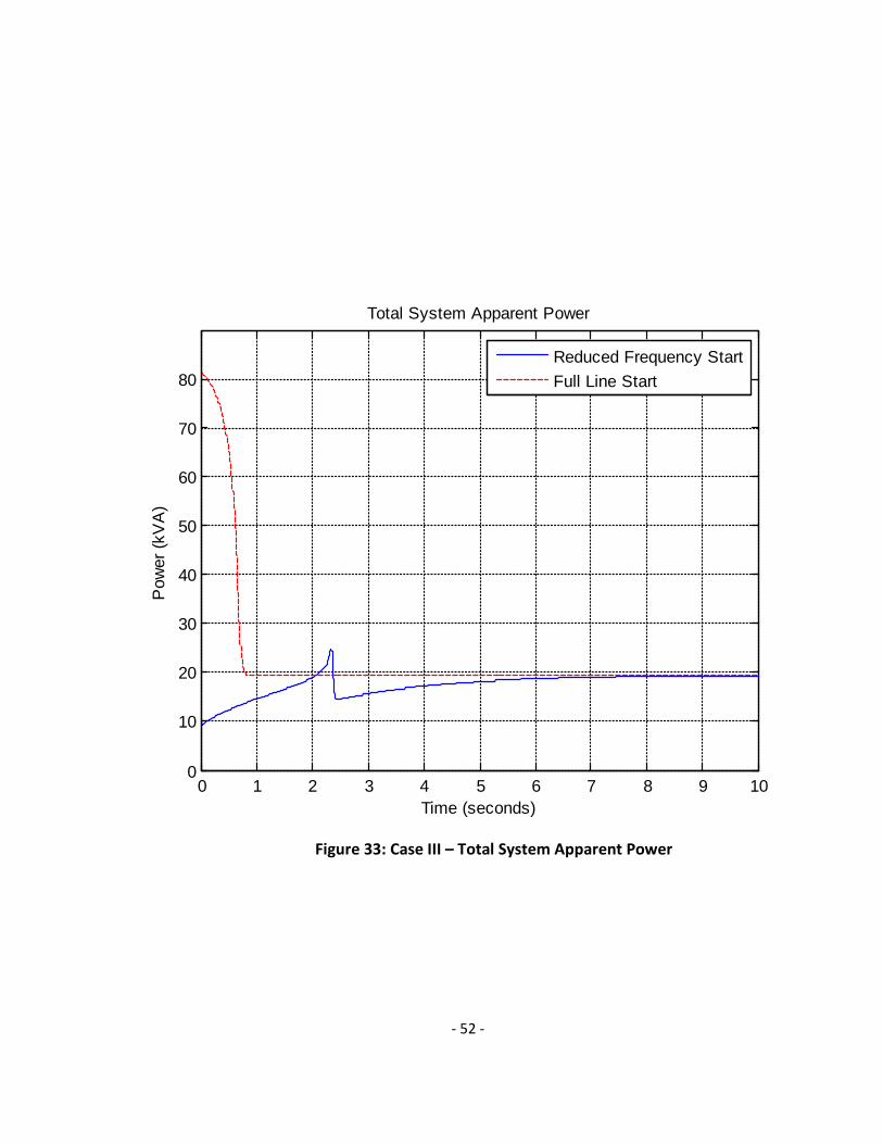
Case III: 20 hp pump only

The final case in this study involves a system that contains only the 20 hp pump.

Figures 29-33 show the excitation and terminal voltages, motor current, motor speed,

system average power input and system apparent power input, respectively, for Case III.

The plot that tells the most important story is presented in Figure 33 which shows the

total system apparent power demanded by the system. Again, there are significant

savings when using the technique outlined in this paper. With a full line start, the

maximum apparent power requirement of the system peaks at 81.60 kVA. When using

the reduced frequency technique, the maximum apparent power requirement is 24.68

kVA. In this case, the required apparent power supplied is reduced 70%.

- 48 -

0 1 2 3 4 5 6 7 8 9 100

50

100

150

200

250

300

350

400

Excitation Voltage (Ef) and Terminal Voltage (V1)

Time (seconds)

Vol

ts

EfV1

Figure 29: Case III – Excitation and Terminal Voltages

- 49 -

0 1 2 3 4 5 6 7 8 9 100

20

40

60

80

100

Motor Current

Time (seconds)

Cur

rent

(per

pha

se)


Figure 30: Case III – Current into the Motor

- 50 -

0 1 2 3 4 5 6 7 8 9 100

500

1000

1500

2000

2500

3000

Motor Shaft Speed

Time (seconds)

Spe

ed(n

m)


Figure 31: Case III – Motor Shaft Speed

- 51 -

0 1 2 3 4 5 6 7 8 9 100

5

10

15

20

25

30

35


Time (seconds)

Pow

er (k

W)


Figure 32: Case III – Total System Real Power

- 52 -

0 1 2 3 4 5 6 7 8 9 100

10

20

30

40

50

60

70

80


Time (seconds)

Pow

er (k

VA

)


Figure 33: Case III – Total System Apparent Power

- 53 -

Critical Points

As shown in the previous figures, the key plot illustrating the effectiveness of the

technique is the required power to operate the system. There is a critical region within

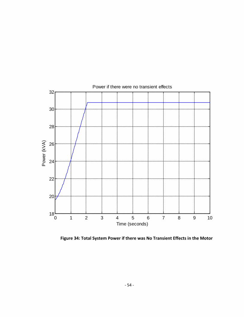
which one can work in order to optimize the utilization of the system. In Figure 34, is an

approximate plot of what the required power of a system using the technique would be

if there was no initial spike in current due to the starting of the motor. The area that lies

below the steady state power requirement (30.76 kVA in this case) during startup is a

“free power region.” There is no appreciable benefit to keeping the required power

below the steady state power level, especially if in doing so causes more disturbances in

the electrical service.

Using Case II with the 10 kW parallel load with a starting generator speed of 600

rpm (40% synchronous speed), it is evident that the initial spike of kVA required is the

limiting factor as seen in Figure 24. It is also evident that at a starting speed of 600 rpm

in both Cases I and II, that the peak of the inrush kVA spike exists below the level found

when starting with full voltage and frequency. In particular, the peak of the kVA demand

spike in Case I is less than the steady state power requirement of the system. When this

occurs, it is an indication that the respective starting speed of 600 rpm is lower than

what is necessary. This is significant in that, as mentioned in the statement of the

problem, as the starting speed is further lowered, there is introduced more

dimming/flickering of the lights and general variation of power flow. In order to

- 54 -

Figure 34: Total System Power if there was No Transient Effects in the Motor

0 1 2 3 4 5 6 7 8 9 1018

20

22

24

26

28

30

32Power if there were no transient effects

Pow

er (k

VA

)

Time (seconds)

- 55 -

optimize the use of the technique, one must discover a way to maximize the use of the

“free power region.” Again, I call this the “free power region” because the system is

equipped to handle loads in this region at and below the steady state power

requirement. Thus it is fruitless to try to attain savings below this point, especially if it is

at the expense of the performance of anything else in the system.

As previously articulated, there is an optimal starting point that will yield

favorable power flow dynamics while minimizing the reduction of the speed of the

generator. This optimized starting point will be referred to as the “critical point.” This

critical point can be discovered by running the model using incremental values for the

starting generator speed (the amount the rack is pulled back).

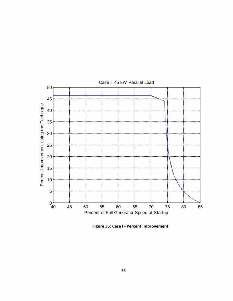
First, Case I is evaluated. Figure 35 shows the percent improvement (reduction in

maximum required generator apparent power) in the system using the technique versus

the percentage of synchronous speed that the generator engine is reduced to. Looking

at the plot, it is evident that reducing the speed below the critical point of 70% of

synchronous speed is pointless. Figure 36 shows the power consumption of the system

when the critical point is utilized.

- 56 -

Figure 35: Case I - Percent Improvement

40 45 50 55 60 65 70 75 80 850

5

10

15

20

25

30

35

40

45

50

Per

cent

Impr

ovem

ent u

sing

the

Tech

niqu

e

Percent of Full Generator Speed at Startup

Case I: 45 kW Parallel Load

- 57 -

Figure 36: Case I – System Power with the Critical Point Utilized

0 1 2 3 4 5 6 7 8 9 100

20

40

60

80

100

120

140


Time (seconds)

Pow

er (k

VA

)


- 58 -

It is evident that the critical point is where the peak of the kVA demand during inrush is

equal to the steady state power requirement of the system.

Next, Case II is explored. Figure 37 shows the percent improvement in the

system using the technique versus the percentage of synchronous speed to which the

generator engine is reduced. Looking at the plot, it is evident that reducing the speed

below the critical point of 49% of synchronous speed is pointless. Figure 38 shows the

power consumption of the system when the critical point is utilized.

Finally, Case III is explored. Looking at Figure 33, it appears that reducing the

speed below 40% of synchronous speed may further improve the performance.

However, because lowering the generator speed below 40% compromises the system

ability to provide adequate torque to start the pump, thus is not considered an option

and the minimum of 40% would be considered its critical point. Again, Figure 33 has

already illustrated the power consumption of the system when the critical point is

utilized.

- 59 -

Figure 37: Case II - Percent Improvement

40 45 50 55 60 65 70 75 80 850

10

20

30

40

50

60

70

Percent of Full Generator Speed at Startup

Per

cent

Impr

ovem

ent u

sing

the

Tech

niqu

e

Case II: 10 kW Parallel Load

- 60 -

Figure 38: Case II – Total System Power with the Critical Point Utilized

0 1 2 3 4 5 6 7 8 9 100

10

20

30

40

50

60

70

80

90

100


Time (seconds)

Pow

er (k

VA

)


- 61 -

Generator Excitation Type

As mentioned in Chapter 3, there is a choice to be made concerning which type

of generator to choose for this situation. The choices mentioned were separately

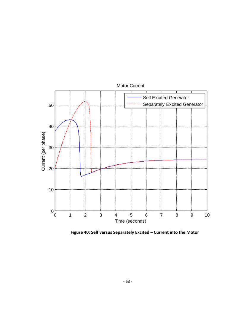
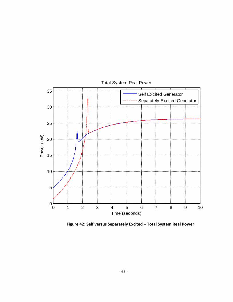
excited and self excited. By comparing system performance using the two different

types of excitation, it becomes an easy decision to select the self excited generator. This

improved performance occurs due to the shape of its respective voltage-frequency

curve, including the fact that the self excited generator provides a higher initial terminal

voltage. This makes the amount of change required, from the initial voltage to the final

voltage, smaller while still being low enough to help offset the transient spike in current

at a poor power factor. Its characteristically linear increase in excitation voltage (shown

in Figure 18) manages the motor load in more consistent and steady manor as opposed

to the parabolic increase (shown in figure 17) that occurs with a separately excited

generator. Figures 39-43 illustrate the difference in performance of the two types using

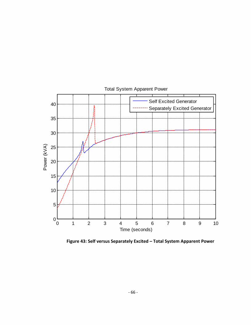
system setup in Case II.

- 62 -

Figure 39: Self versus Separately Excited – Terminal Voltage

0 1 2 3 4 5 6 7 8 9 100

50

100

150

200

250

Terminal Voltage

Time (seconds)

Vol

tage

(per

pha

se)

Self Excited GeneratorSeparately Excited Generator

- 63 -

0 1 2 3 4 5 6 7 8 9 100

10

20

30

40

50

Motor Current

Time (seconds)

Cur

rent

(per

pha

se)


Figure 40: Self versus Separately Excited – Current into the Motor

- 64 -

0 1 2 3 4 5 6 7 8 9 100

500

1000

1500

2000

2500

3000

Motor Shaft Speed

Time (seconds)

Spe

ed(n

m)


Figure 41: Self versus Separately Excited – Motor Shaft Speed

- 65 -

0 1 2 3 4 5 6 7 8 9 100

5

10

15

20

25

30

35


Time (seconds)

Pow

er (k

W)


Figure 42: Self versus Separately Excited – Total System Real Power

- 66 -

0 1 2 3 4 5 6 7 8 9 100

5

10

15

20

25

30

35

40


Time (seconds)

Pow

er (k

VA

)


Figure 43: Self versus Separately Excited – Total System Apparent Power

- 67 -

Chapter 5: Conclusions

As evident from the plots of the results in the previous section, this is certainly

an effective means of reducing the size of a generator to serve the load as laid out in the

problem. Again, it is important to look back on two prominent affects of this solution.

The first would be the great financial benefit that comes with the reduction of

the generator size. As mentioned in an example during the presentation of the problem.

The savings using this technique can end up in the thousands of dollars. That amount of

money saved very well could end up making a project move forward as opposed to

canceled due to budget constraints. Further, in the event that there were available

funds for purchasing an oversized generator, one could use the technique from this

paper to save that money and put it toward other areas in the project.

Secondly, this is a very practical solution. While the quality of the power to the

system is somewhat compromised for a couple of seconds, this is completely acceptable

given the situation in which this is going to be used. As far as execution of the

technique, the process of pulling back the rack and bringing on the motor load is very

simple and most anyone could be trained to perform such a task.

- 68 -

Chapter 6: Recommendation for Future Work

There are several avenues one could pursue in the future building upon what has

been discussed in this paper. This is by no means an exhaustive list, but some

suggestions of what the author would find interesting.

In this paper, the focus is on one pump load along with a given amount of

common loads. While the purpose of the pump in this simulation is to provide much

need water to the community, there are certainly other pumps or other loads that are

driven by large motors. Future studies could investigate the effects of multiple motor

loads at startup with various load characteristics that may differ from the load

characteristic in the centrifugal pump in this paper.

Also, it would be interesting to apply this idea to alternate energy systems such

as wind or solar power. Being able integrate this be even more beneficial than using a

backup generator as discussed in this paper. Use of an alternate energy source would be

more environmentally friendly and would make the community more self reliant, rather

than being at the mercy of the unpredictable utility company. As mentioned in the

presentation of the problem, one of the motivations of the technique in this paper is to

reduce the cost and allow projects to be undertaken. While the cost of diesel generators

are not trivial, the cost savings involved in buying less equipment for alternate energy

sources such as solar panels, battery banks, etc. would be huge as the costs of said

equipment dwarfs the cost of a diesel generator. Using this technique in that situation

would involve reducing the inverter frequency in the same manner as the generator

- 69 -

frequency was reduced in this paper. In certain cases, doing so could decrease the size

of the battery bank needed to provide the startup currents required by the motor.

- 70 -

Mas

terM

odel

.m

WaveIN.m

Developed Torque (TD)

StartSpeed, Time

Frequency

VFcurve.m Frequency

Generator Voltage

InductionMotor.m Voltage, Frequency

PumpTorqueSpeed.m TD, Shaft Speed

Load Torque (TL)

Pump.m

Shaft Speed (next iteration)

TD, TL, Shaft Speed

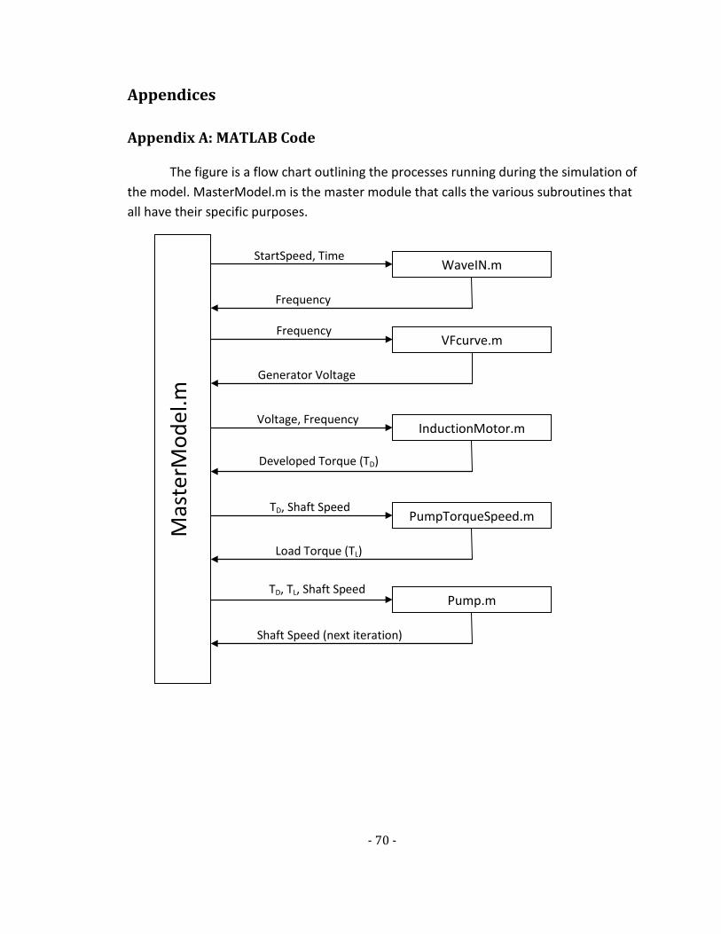
Appendices

Appendix A: MATLAB Code

The figure is a flow chart outlining the processes running during the simulation of the model. MasterModel.m is the master module that calls the various subroutines that all have their specific purposes.

- 71 -

MasterModel.m % Taylor Begley % MasterModel.m is the driver of the entire simulation % This file will call the subroutines that will make the % calculations to determine the outcome from the given conditions clear all;close all; disp('Begin Run') global TSTART TSTOP TIME FFULL V1FULL PPL Ef1FULL; %global vars denoted by ALL CAPS PPL = 45*1000; %desired parallel load in watts TSTART = 0; %start time for the simulation TSTOP = 10; %run simulation until time TSTOP (seconds) numpoints = 1000;%number of testpoints TIME = linspace(TSTART,TSTOP,numpoints); FFULL = 50; %frequency when running full gpoles = 4; %number of poles on generator ns = 120*FFULL/gpoles; %synchronous speed (rpm) V1FULL = 460/sqrt(3); %per phase generator voltage (when at full voltage) test=0; global VERSUS STARTSPEED % for STARTSPEED = 1:31 STARTSPEED=00; Ef1FULL=514.2; %Separately Excited %514.2for 75/45;435 for 45/10; %Self Excited %434.35 for 35/10;514.2 for 75/45; %389.58 for 30/0.0000000001 Gen=75000% kVA generator Ilb=Gen/(460*sqrt(3)); Zb=(V1FULL)/Ilb; Xs=1.0*Zb; Ls=Xs/(2*pi*50); for VERSUS=1:2 % Gen=35000% kVA generator % Ilb=Gen/(460*sqrt(3)) % Zb=(V1FULL)/Ilb % Xs=1.0*Zb

- 72 -

% Ls=Xs/(2*pi*50) for k = 1 : numpoints ne(k) = WaveIN(TIME(k),ns); fe(k) = ne(k)*gpoles/120;%fe(k)=42.5; V1t(k) = VFcurveEf(fe(k)); if k==1 nm(1)=0;wm(1)=0; Zboth(k)=V1finder(fe(k),nm(k));%finds Zboth else nm(k)=(60/(2*pi))*wm(k); Zboth(k)=V1finder(fe(k),nm(k));%finds Zboth end Ztotal(k)=j*2*pi*fe(k)*Ls + Zboth(k);%j*wm(k)*Ls + Zboth(k); Itotal(k)=V1t(k)/Ztotal(k); Vs(k)=Itotal(k)*j*2*pi*fe(k)*Ls;%Itotal(k)*j*wm(k)*Ls; V1(k)=abs(V1t(k)-Vs(k)); if VERSUS==2 V1(k)=VFcurve(fe(k)); end if fe(k) >= .85*50 V1(k)=VFcurve(fe(k)); V1t(k)=abs(V1(k)/Zboth(k)*j*2*pi*fe(k)*Ls + V1(k)); end if k==1 nm(1)=0;wm(1)=0; TTdandI1 = InductionMotor(V1(k),fe(k),nm(k)); else nm(k)=(60/(2*pi))*wm(k); TTdandI1 = InductionMotor(V1(k),fe(k),nm(k-1)); end TTd(k) = TTdandI1(1);I1(k) = TTdandI1(2);TPin(k) = TTdandI1(3); IReIm(k) = TTdandI1(4);kVAin(k) = TTdandI1(5); TL(k) = PumpTorqueSpeed(nm(k),TTd(k)); if k < numpoints wm(k+1) = Pump(TTd(k),TL(k),wm(k),[TIME(k) TIME(k+1)]); end PP=ParallelLoad(V1(k),fe(k)); Ipl(k)=PP(1);PPow(k)=PP(2); % k % pause; Iph(k)=IReIm(k)+Ipl(k)/3; if fe(k) > 42.5

- 73 -

if test ==0 jwLs(k)=j*.85*50*2*pi*Ls; VjwLs(k)=(Iph(k)).*jwLs(k); V85=VjwLs(k); test = 1 else VjwLs(k) =V85; end else jwLs(k)=j*fe(k)*2*pi*Ls; VjwLs(k)=(Iph(k)).*jwLs(k); end tests(k)=test; Ef(k)=V1(k)+VjwLs(k); end Itot=I1+real(Ipl); Isys=IReIm+Ipl; PFsys=cos(angle(Isys)); if VERSUS == 1 c='b-'; else c='r--';end rfs='Reduced Frequency Start'; fls='Full Line Start'; figure(1) %plot Generator speed output plot(TIME,ne,c) axis([TSTART TSTOP 0 ns*1.1]);title('Generator speed'); xlabel('Time (seconds)');ylabel('Speed (rpm)');grid on; hold on;legend(rfs,fls) if VERSUS ==1 figure(2) %plot characteristic Voltage-Frequency Curve % ftest = linspace(min(fe),FFULL,50); % for char = 1:length(ftest) % VFchar(char) = VFcurveEf(ftest(char)); % end % plot(ftest,VFchar,c); title('Separately Excited Generator Characteristic Curve'); plot(fe,V1t,c); title('Self Excited Generator Characteristic Curve'); xlabel('Frequency (Hz)');ylabel('Excitation Voltage (per phase)');grid on;axis([20 42.5 200 550]); end % hold on;legend(rfs,fls)

- 74 -

figure(3) %plot voltage regulated V1 V1x(VERSUS)=max(abs(V1)); plot(TIME,abs(V1),c) axis([TSTART TSTOP 0 max(V1x)*1.1]);title('Voltage V1'); xlabel('Time (seconds)');ylabel('Voltage (per phase)');grid on; hold on;legend(rfs,fls) figure(4) %plot motor current plot(TIME,abs(I1),c) axis([TSTART TSTOP 0 max(abs(I1))*1.1]);title('Motor Current'); xlabel('Time (seconds)');ylabel('Current (per phase)');grid on; hold on;legend(rfs,fls) figure(5) %plot developed Torque plot(TIME,TTd,c) axis([TSTART TSTOP 0 max(TTd)*1.1]);title('Developed Torque'); xlabel('Time (seconds)');ylabel('Torque');grid on; hold on;legend(rfs,fls) figure(6) %plot load Torque plot(TIME,TL,c) axis([TSTART TSTOP 0 max(TL)*1.1]);title('Load Torque'); xlabel('Time (seconds)');ylabel('Torque');grid on; hold on;legend(rfs,fls) figure(7) %plot accelerating Torque plot(TIME,TTd-TL,c) axis([TSTART TSTOP 0 max(TTd-TL)*1.1]);title('Accelerating Torque'); xlabel('Time (seconds)');ylabel('Torque');grid on; hold on;legend(rfs,fls) figure(8) %plot nm plot(TIME,nm,c) axis([TSTART TSTOP 0 max(nm)*1.1]);title('Motor Shaft Speed'); xlabel('Time (seconds)');ylabel('Speed(nm)');grid on; hold on;legend(rfs,fls) figure(9) %plot Power into motor TPin=TPin; plot(TIME,TPin/1000,c) axis([TSTART TSTOP 0 max(TPin/1000)*1.1]);title('Real Power into Motor'); xlabel('Time (seconds)');ylabel('Power(kW)');grid on; hold on;legend(rfs,fls)

- 75 -

TPin(numpoints) figure(10) %plot Power into motor plot(TIME,kVAin/1000,c) axis([TSTART TSTOP 0 max(kVAin/1000)*1.1]);title('Apparent Power into Motor'); xlabel('Time (seconds)');ylabel('Power(kVA)');grid on; hold on;legend(rfs,fls) TPin(numpoints) figure(11) %plot Power Tw PowerTw=TTd.*wm; plot(TIME,PowerTw/1000,c) axis([TSTART TSTOP 0 max(PowerTw/1000)*1.1]);title('Power TTd*wm to Pump'); xlabel('Time (seconds)');ylabel('Power(kW)');grid on; hold on;legend(rfs,fls) PowerTw(numpoints) % figure(12) %plot motor efficiency % eff=PowerTw./TPin*100; % plot(TIME,eff,c) % axis([TSTART TSTOP 0 max(eff)*1.1]);title('Motor Efficiency PowerTw/PowerVI'); % xlabel('Time (seconds)');ylabel('Efficiency %');grid on; % hold on;legend(rfs,fls) SteadyStateShaftSpeed=wm(numpoints)*30/pi % figure(13) %plot Power current * % PPo=PPo./1000;%voltage power in kVA % plot(TIME,PPo,c) % axis([TSTART TSTOP 0 max(PPo)*1.1]);title('PPo'); % xlabel('Time (seconds)');ylabel('Power(kW)');grid on; % hold on;legend(rfs,fls) % max(PPo) % figure(14) %Parallel load current % plot(TIME,real(Ipl),c) % axis([TSTART TSTOP 0 max(Ipl)*1.1]);title('Parallel Load Current'); % xlabel('Time (seconds)');ylabel('Current');grid on; % hold on;legend(rfs,fls) figure(15) %Parallel load Power Powerpl=real(Ipl.*V1); Powerpl=real(PPow); Powerpl=abs(V1).*abs(Ipl).*cos(angle(V1)-angle(Ipl));

- 76 -

PPx(VERSUS)=max(abs(Powerpl)); plot(TIME,(Powerpl/1000),c) axis([TSTART TSTOP 0 max(PPx/1000)*1.1]);title('Parallel Load Real Power'); xlabel('Time (seconds)');ylabel('Power (kW)');grid on; hold on;legend(rfs,fls) figure(16) %Total System Power PowerSYS=Powerpl+TPin; plot(TIME,PowerSYS/1000,c) axis([TSTART TSTOP 0 max(PowerSYS/1000)*1.1]);title('Total System Real Power'); xlabel('Time (seconds)');ylabel('Power (kW)');grid on; hold on;legend(rfs,fls) figure(17) %Total System kVA kVASYS=abs(Powerpl/0.85+kVAin); plot(TIME,kVASYS/1000,c) axis([TSTART TSTOP 0 max(kVASYS/1000)*1.1]);title('Total System Apparent Power'); xlabel('Time (seconds)');ylabel('Power (kVA)');grid on; hold on;legend(rfs,fls) % figure(18) %Total System Power Factor % plot(TIME,PFsys,c) % axis([TSTART TSTOP 0 1]);title('Total System Power Factor'); % xlabel('Time (seconds)');ylabel('Power Factor');grid on; % hold on;legend(rfs,fls) figure(18) %Parallel load Power plot(TIME,((Powerpl/.85)/1000),c) axis([TSTART TSTOP 0 max((PPx/.85)/1000)*1.1]);title('Parallel Load Apparent Power'); xlabel('Time (seconds)');ylabel('Power (kVA)');grid on; hold on;legend(rfs,fls) % figure(19) %Power Ratio of Motor Power/Total Power % PowerRatio=TPin./PowerSYS; % plot(TIME,PowerRatio*100,c) % axis([TSTART TSTOP 0 100]);title('Motor Power/System Power'); % xlabel('Time (seconds)');ylabel('Ratio (%)');grid on; % hold on;legend(rfs,fls) figure(20)%plot Ef versus V1 if VERSUS ==1 plot(TIME,V1t,'b');hold on plot(TIME,abs(V1),'r--'); axis([TSTART TSTOP 0 max(V1t)*1.1]);title('Excitation Voltage (Ef) and Terminal Voltage (V1)');

- 77 -

xlabel('Time (seconds)');ylabel('Volts');grid on; legend('Ef','V1') end PC(VERSUS)=max(kVASYS); end%VERSUS MAXkVA_With_Without_Ratio_PPL=[PC(1)/1000 PC(2)/1000 PC(1)/PC(2) (V1FULL*real(Ipl(numpoints)))/1000] WaveIN.m

% This m-file is going to give a wafeform into the system % based on the pulling back of the rack on the diesel generator % Given a time (t), it will output ne (electrical speed) function [ne] = WaveIN(t,ns) global VERSUS STARTSPEED initspeed = (STARTSPEED+40)/100*ns;%Initial speed at Time Zero if VERSUS == 1 ne = ns -(ns-initspeed)*exp(-t/1.5); else ne=ns; end VFcurve.m

% This m-file is called by MasterModel.m and is the representative % voltage-frequency curve that portrays voltage regulation % input frequency, output is the voltage function [V1] = VFcurve(f) global V1FULL FFULL; fmin = .85 * FFULL; if f >= fmin V1 = V1FULL; else % V1 = (V1FULL / fmin) * f;%self excited V1 = V1FULL/fmin^2 * f^2;%separately excited

- 78 -

end InductionMotor.m

% InductionMotor.m - calculates induction motor performance ( I1, PF, % 3Td, Ps, efficiency ) based on equivalent circuit % Reads equivalent circuit parameters from im_data.m function [TTdandI1] = InductionMotor(V1,f,nm) IM_DATA, global V1FULL FFULL;% p=4; % Phase voltage, frequency, poles poles=2; ns = 120*f/poles; %synchronous speed (rpm) based on current freq ws=2/poles*2*pi*f; s = (ns-nm)/ns; % Slip Pfw=700; Tfw= (Pfw*(30/pi)/2900)*(1-s); % Empirical adjustment of R2pr & X2pr for fr variation R2pr0=R2pr; X2pr0=X2pr; smax=R2pr/sqrt(R1^2+(X1+X2pr)^2); if s > smax R2pr=(0.5+0.5*sqrt(s/smax))*R2pr0; X2pr=(0.4+0.6*sqrt(smax/s))*X2pr0; else; R2pr=R2pr0; X2pr=X2pr0; end Z2 = R2pr/s+j*X2pr; Zm=j*Rc*Xm/(Rc+j*Xm); Zin = R1+j*X1 + Z2*Zm/(Z2+Zm); I11 = V1/Zin; I1 = abs(I11); PF = cos(angle(I11)); I2pr = abs(Zm/(R2pr/s+j*X2pr+Zm)*I11); TPin = 3*V1*I1*PF; TTd = 3*I2pr^2*R2pr/s/ws; nm=(1-s)*ns; TTout = TTd - (Tfw); kVAin=TPin/PF; PPo=TTd*(1-s)*ws - Pfw*(nm/ns)^n; TTdandI1=[TTout I1 TPin I11 kVAin];

- 79 -

IM_DATA.m

% IM_DATA.m - contains induction motor equivalent circuit % parameter values to be read by calling program. m=1.17; R1=0.1*m; R2pr=.32*m; X1=1.30*m; X2pr=1.35*m; Rc=330*m; Xm=27.59512*m;

PumpTorqueSpeed.m

% PumpTorqueSpeed.m inputs the current speed and developed torque % uses a characteristic Torque-Speed curve of centrifugal pump % to output the load torque after making sure that the load torque % does not exceed the developed torque function [TL] = PumpTorqueSpeed(nm,Td) wm = nm * (pi/30); %below is the calculated parabola to fit %the pumps speed torque characteristic TL = 0.000006866825208085613*(wm.*30/pi)^2-0.007603448275862068*(wm*30/pi)+6.3; %check to ensure load torque does not exceed developed torque if TL > Td disp('******Load torque(TL) exceeds developed torque(Td)******') end Pump.m % Pump.m function [wm_next] = Pump(Td,TL,wm,tspan) J = .1547; %Define the pumps inertia FW=6; %beta*wm for the rated speed beta = FW/(3000*pi/30);

- 80 -

% define the diff equ in the form w' = C1 + C2*w global C1 C2; C1 = (Td-TL)/J; C2 = -beta/J; [t,wm_n] = ode23('PumpODE',tspan,wm); wm_next=wm_n(length(wm_n)); PumpODE.m

% PumpODE.m function wmprime = PumpODE(t,wm); global C1 C2; wmprime = C1 + C2*wm;

ParallelLoad.m

% ParallelLoad.m is the load that is % in parallel with the motor/pump load % this is to power lighting, rcpts, fans, etc. % This will take the load on a per phase basis % and out put the total requirement (phases balanced) function [Ipl] = ParallelLoad(V1) global V1FULL PPL pf = 0.85;% Power Factor of the load Ir=PPL/V1/3; Pperphase=PPL/3; R=.7225*(V1FULL^2)/Pperphase; X=tan(acos(pf))*R; I=V1/(R+j*X); Ipl=3*I;

- 81 -

Appendix B: Centrifugal Pump Data

References

- 82 -

References

1. Pettigrew, Dana R. Variable Frequency Generator as a Power Supply for an ESP. Houston : ESP Workshop, 2005.

2. Alger, Philip L. Induction Machines: Their Behavior and Uses. New York : Gordon and Breach Science Publishers, 1970. Chapter 8.

3. Lobanoff, Val S. and Ross, Robert R. Centrifugal Pumps: Design and Application. Houston : Gulf Publishing, 1992.

4. Wylie, E. Benjamin, Streeter, Victor L. and Suo, Lisheng. Fluid Transients in Systems. New York : Prentice Hall, 1993.

- 83 -

Vita

Name: Taylor Andew Begley

Birth: December 13, 1982 Danville, Kentucky

Education: 2005 B.S.E.E. from the University of Kentucky

Professional: Electrical Engineer, Mason & Hanger, Lexington, KY

REDUCED FREQUENCY MOTOR STARTING FOR THIRD WORLD …

Documents

Transcript of REDUCED FREQUENCY MOTOR STARTING FOR THIRD WORLD …