Rebayes: an R package for empirical bayes mixture methods

Rebayes: an R package for empirical bayes mixture methods

Roger KoenkerJiaying Gu

The Institute for Fiscal Studies Department of Economics, UCL

cemmap working paper CWP37/17

REBAYES:

AN R PACKAGE FOR EMPIRICAL BAYES MIXTURE METHODS

ROGER KOENKER AND JIAYING GU

Abstract. Models of unobserved heterogeneity, or frailty as it is commonly known in survival

analysis, can often be formulated as semiparametric mixture models and estimated by maxi-

mum likelihood as proposed by Robbins (1950) and elaborated by Kiefer and Wolfowitz (1956).Recent developments in convex optimization, as noted by Koenker and Mizera (2014b), have

led to dramatic improvements in computational methods for such models. In this vignette we

describe an implementation contained in the R package REBayes with applications to a widevariety of mixture settings: Gaussian location and scale, Poisson and binomial mixtures for

discrete data, Weibull and Gompertz models for survival data, and several Gaussian models in-

tended for longitudinal data. While the dimension of the nonparametric heterogeneity of thesemodels is inherently limited by our present gridding strategy, we describe how additional fixed

parameters can be relatively easily accommodated via profile likelihood. We also describe somenonparametric maximum likelihood methods for shape and norm constrained density estimation

that employ related computational methods.

1. Introduction

Empirical Bayes methods as conceived by Robbins (1956) are enjoying a robust revival stim-ulated by more bountiful data sources and new theoretical developments exemplified by Efron(2010). Mixture models have played a central role in this revival, and this has sparked renewed in-terest in the Kiefer and Wolfowitz (1956) nonparametric maximum likelihood estimator (NPMLE)for mixtures. Relatively recent developments in convex optimization have dramatically improvedcomputational methods for the Kiefer-Wolfowitz NPMLE, as described in Koenker and Mizera(2014b). To make these methods accessible to the research community we have developed an Rpackage REBayes that incorporates a wide variety of nonparametric mixture models and providesKiefer-Wolfowitz procedures for each of them.

The simplest univariate mixture model takes the form,

g(x) =

∫ϕ(x, θ)dF (θ),

where ϕ is a known density, that we will refer to as the base density, and F is an unknowndistribution function that we would like to estimate, given an iid sample from the mixture densityg. The most familiar example would be the Gaussian location model with ϕ standard Gaussian,so,

g(x) =

∫ϕ(x− µ)dF (µ).

This is the standard Gaussian sequence model and has been studied in many simulation exper-iments, including Johnstone and Silverman (2004), Martin and Walker (2013) and Castillo andvan der Vaart (2012), and employed in many – typically genomic – applications. The objective ofsuch analyses is a compound decision problem: Given an exchangeable sample, X1, ...Xn estimatethe corresponding µ1, ...µn subject to quadratic loss. As noted by Robbins (1956) this yields theoptimal Bayes rule,

(1) E(µ|x) = x+ g′(x)/g(x).

Efron (2011) calls this Tweedie’s formula since Robbins attributes it to M.C.K. Tweedie, howeverit appears earlier in Dyson (1926) who credits it to the English astronomer Arthur Eddington.

Version: February 24, 2016. This research was partially supported by NSF grant SES-11-53548.

1

2 ROGER KOENKER AND JIAYING GU

To turn this into a practical shrinkage formula we obviously need to choose an estimator forthe mixture density g. Much of the earlier literature on this problem may be viewed as offeringparametric empirical Bayes proposals in which F is specified up to a finite dimensional vector ofhyperparameters.

More recently interest has focused on nonparametric estimation of the mixing distribution asin Efron (2011), Brown and Greenshtein (2009) and Jiang and Zhang (2009). The latter authorsproposed using the Kiefer-Wolfowitz NPMLE to estimate F , and thereby g, and then to usethe Tweedie formula. The main drawback of this proposal was the painfully slow convergenceof the fixed point iteration of the EM algorithm used to compute the NPMLE. Koenker andMizera (2014b), observing that the discretization suggested by Jiang and Zhang (2009) produceda convenient, finite dimensional convex optimization problem showed that the NPMLE could beimplemented much more efficiently by standard interior point methods. In the next section we willbriefly describe this implementation, and then turn to descriptions of various applications. Otherrecent applications of the REBayes package may be found in Dicker and Zhao (2014) and Jiangand Zhang (2015).

2. Computation of the Kiefer-Wolfowitz NPMLE

It is easy to see that the primal problem

(2) minF∈F{−

n∑i=1

log g(xi) | g(xi) =

∫ϕ(xi, θ)dF (θ), i = 1, ..., n},

where F denotes the set of all mixing distributions, is a convex program. We seek to minimizea strictly convex objective function subject to linear equality constraints over the convex set, F .The dual formulation of the problem is also illuminating.

Theorem 1. (Koenker and Mizera (2014b)) The solution, F , of (2) exists, and is an atomic

probability measure, with not more than n atoms. The locations, µj, and the masses, fj, at theselocations can be found via the following dual characterization: the solution, ν, of

(3) max{n∑i=1

log νi |n∑i=1

νiϕ(Yi, µ) ≤ n for all µ}

satisfies the extremal equations (n equations in less than n variables)

(4)∑j

ϕ(Yi, µj)fj =1

νi,

and µj are exactly those µ where the dual constraint is active—that is, the constraint function in(3) is equal to n.

The dual formulation reduces the objective function to a simple finite dimensional sum, albeitnow with an infinite dimensional constraint. The upper bound of n on the number of atoms,established under slightly stronger conditions by Lindsay (1983), encourages us in the quest fora discrete formulation. We should hasten to add that we have no assurances about where theseatoms occur, in particular it is clear already from an example in Laird (1978) that they need notoccur at the observed xi. Laird (1978) proposed using the EM algorithm to solve a discretizationof the primal problem (2) and subsequent authors, notably Heckman and Singer (1984) and Jiangand Zhang (2009), have followed her lead. However, as has been frequently observed, EM canbe quite lethargic in its pursuit of the optimum. Koenker and Mizera (2014b) describe somecomparisons of a fixed point EM algorithm with the interior point method implemented in Mosek.For a relatively small Gaussian location mixture problem with n = 200 and a grid of 300 pointsfor the mixing distribution for µ, the interior point method produced a very precise solution inabout 1 second and 15 iterations, while after 10 minutes and 100,000 iterations the EM algorithmwas still struggling to obtain the same accuracy as the interior point solution.

In our discrete formulation we consider a fixed grid, {u1, ..., um}, of potential support pointsfor the mixing distribution, F . Typically, m is a few hundred, and the grid is equally spaced, but

REBAYES: AN R PACKAGE FOR EMPIRICAL BAYES MIXTURE METHODS 3

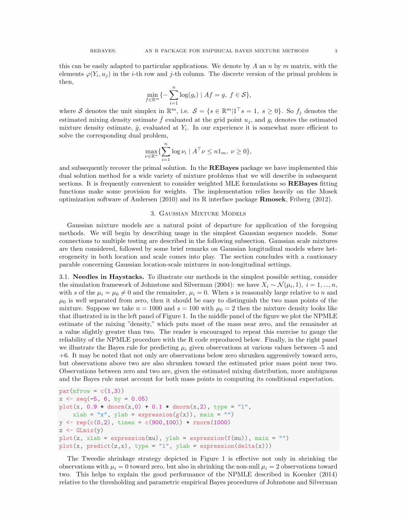
this can be easily adapted to particular applications. We denote by A an n by m matrix, with theelements ϕ(Yi, uj) in the i-th row and j-th column. The discrete version of the primal problem isthen,

minf∈Rm

{−n∑i=1

log(gi) | Af = g, f ∈ S},

where S denotes the unit simplex in Rm, i.e. S = {s ∈ Rm|1>s = 1, s ≥ 0}. So fj denotes the

estimated mixing density estimate f evaluated at the grid point uj , and gi denotes the estimatedmixture density estimate, g, evaluated at Yi. In our experience it is somewhat more efficient tosolve the corresponding dual problem,

maxν∈Rn{n∑i=1

log νi | A>ν ≤ n1m, ν ≥ 0},

and subsequently recover the primal solution. In the REBayes package we have implemented thisdual solution method for a wide variety of mixture problems that we will describe in subsequentsections. It is frequently convenient to consider weighted MLE formulations so REBayes fittingfunctions make some provision for weights. The implementation relies heavily on the Mosekoptimization software of Andersen (2010) and its R interface package Rmosek, Friberg (2012).

3. Gaussian Mixture Models

Gaussian mixture models are a natural point of departure for application of the foregoingmethods. We will begin by describing usage in the simplest Gaussian sequence models. Someconnections to multiple testing are described in the following subsection. Gaussian scale mixturesare then considered, followed by some brief remarks on Gaussian longitudinal models where het-erogeneity in both location and scale comes into play. The section concludes with a cautionaryparable concerning Gaussian location-scale mixtures in non-longitudinal settings.

3.1. Needles in Haystacks. To illustrate our methods in the simplest possible setting, considerthe simulation framework of Johnstone and Silverman (2004): we have Xi ∼ N (µi, 1), i = 1, ..., n,with s of the µi = µ0 6= 0 and the remainder, µi = 0. When s is reasonably large relative to n andµ0 is well separated from zero, then it should be easy to distinguish the two mass points of themixture. Suppose we take n = 1000 and s = 100 with µ0 = 2 then the mixture density looks likethat illustrated in in the left panel of Figure 1. In the middle panel of the figure we plot the NPMLEestimate of the mixing ”density,” which puts most of the mass near zero, and the remainder ata value slightly greater than two. The reader is encouraged to repeat this exercise to gauge thereliability of the NPMLE procedure with the R code reproduced below. Finally, in the right panelwe illustrate the Bayes rule for predicting µi given observations at various values between -5 and+6. It may be noted that not only are observations below zero shrunken aggressively toward zero,but observations above two are also shrunken toward the estimated prior mass point near two.Observations between zero and two are, given the estimated mixing distribution, more ambiguousand the Bayes rule must account for both mass points in computing its conditional expectation.

par(mfrow = c(1,3))

x <- seq(-5, 6, by = 0.05)

plot(x, 0.9 * dnorm(x,0) + 0.1 * dnorm(x,2), type = "l",

xlab = "x", ylab = expression(g(x)), main = "")

y <- rep(c(0,2), times = c(900,100)) + rnorm(1000)

z <- GLmix(y)

plot(z, xlab = expression(mu), ylab = expression(f(mu)), main = "")

plot(x, predict(z,x), type = "l", ylab = expression(delta(x)))

The Tweedie shrinkage strategy depicted in Figure 1 is effective not only in shrinking theobservations with µi = 0 toward zero, but also in shrinking the non-null µi = 2 observations towardtwo. This helps to explain the good performance of the NPMLE described in Koenker (2014)relative to the thresholding and parametric empirical Bayes procedures of Johnstone and Silverman


−4 −2 0 2 4 6

0.0

0.1

0.2

0.3

x

g(x)

−2 0 2 40

510

1520

25

µ

f(µ)

−4 −2 0 2 4 6

0.0

0.5

1.0

1.5

2.0

x

δ(x)

Figure 1. Kiefer Wolfowitz Estimation of a Gaussian Location Mixture: Theleft panel is the (unknown) two component mixture density, the middle panel isthe estimated NPMLE mixing density and the right panel is the estimated Bayesrule for predicting µ = δ(x) based on seeing an observation x.

(2004), Martin and Walker (2013) and Castillo and van der Vaart (2012). These competitors arequite good at shrinking the null observations toward zero, unlike the NPMLE they know that thereis mass at zero, but they tend to leave the non-null observations alone and this tends to inflatetheir mean squared error. This observation raises the natural question how would the NPMLE dowhen the non-null observations came from a more diffuse distribution?

In Figure 2 we illustrate similar performance for a Gaussian location mixture in which 200 ofthe 1000 observations have µi’s drawn from a N (2, 1) distribution. The true mixture density looksquite similar to the prior example, but the NPMLE now identifies three distinct mass points, onelarge one near zero, a smaller one near two and a very small mass point at about 4.5. The Bayesrule is still quite sure that negative xi should be pulled toward zero, and observations near twoare nudged toward two. But despite its small mass the upper mass point of the estimated mixingdistribution exerts a substantial effect. Only when we see extremely large observations biggerthan 4.5 are they pulled back toward this largest mass point. This example is considerably morechallenging than the previous one, but nevertheless the empirical Tweedie formula produced bythe NPMLE provides a reasonable approach.

par(mfrow = c(1,3))

x <- seq(-5, 7, by = 0.05)

plot(x, 0.8 * dnorm(x,0) + 0.2 * dnorm(x,2,sqrt(2)), type = "l",

xlab = "x", ylab = "g(x)", main = "")

y <- c(rep(0,800), rnorm(200, 2)) + rnorm(1000)

z <- GLmix(y)

plot(z, xlab = expression(mu), ylab = expression(f(mu)), main = "")

plot(x, predict(z,x), type = "l", ylab = expression(delta(x)))

3.2. Gaussian Mixtures and Multiple Testing. Robbins (1951) introduced compound deci-sion making with the following (deceptively) simple problem. Suppose we observe,

(5) Yi = θi + ui, i = 1, · · · , n,

with {ui} iid standard Gaussian, and we know that the θi take values ±1. The objective is toestimate the n-vector, θ ∈ {−1, 1}n subject to `1 loss,

L(θ, θ) = n−1n∑i=1

|θi − θi|.


−4 −2 0 2 4 6

0.00

0.05

0.10

0.15

0.20

0.25

0.30

0.35

x

g(x)

−2 0 2 4 60

510

15

µ

f(µ)

−4 −2 0 2 4 6

01

23

4

x

δ(x)

Figure 2. Kiefer Wolfowitz Estimation of a Gaussian Location Mixture: The leftpanel is the (unknown) mixture density, the middle panel is the estimated NPMLEmixing density and the right panel is the estimated Bayes rule for predictingµ = δ(x) based on seeing an observation x.

He observes that when n = 1 the least favorable version of the problem occurs when we assumethat the θi’s are drawn as independent Bernoulli’s with probability p = 1/2 that θi = ±1, andthen he proceeds to show that this remains true for the general “compound decision” problem withn ≥ 1. The minimax decision rule is thus,

δ1/2(y) = sgn(y)

and yields constant risk,

R(δ1/2, θ) = EL(δ1/2(Y ), θ) = Φ(−1) ≈ 0.1586,

irrespective of p. And yet, something feels wrong with this procedure. If we saw mostly positiveYi’s wouldn’t we begin to think that p 6= 1/2? Why are we so attached to the worst case scenario?Exploiting the common structure of the n problems, Robbins suggests estimating p by p = (y+1)/2.Given this method of moments estimate of p, he suggests plugging it into the decision rule,

δp(y) = sgn(y − 1/2 log((1− p)/p)),

a procedure that follows immediately from the requirement that,

P (θ = 1|x, p) =pϕ(x− 1)

pϕ(x− 1) + (1− p)ϕ(x+ 1),

exceeds one half, that is, that the posterior median of θ be 1. This prototype empirical Bayesprocedure sacrifices a little in performance when p is really near 1/2, but achieves substantial gainsin performance when p differs substantially from 1/2. Of course, when n is large, p → p, so wehave a form of asymptotic optimality.

The link to the multiple testing literature for the Robbins problem is immediately clear sinceestimation of θ ∈ {−1, 1}n is essentially a testing problem in which we have weighed false discoveryand false non-discovery equally. If we treat θ = −1 as the null hypothesis and θ = 1 as thealternative, a p-value procedure based on Ti = 1−Φ(Xi + 1) with cutoff Φ(−1) the decision rule,

δp(T ) = sgn(Φ(−1)− T )

is equivalent to the minimax rule, δ(x) = sgn(x). If, instead, we would like to fix the marginal falsediscovery rate (mFDR) at some level and optimize marginal false nondiscovery rate (mFNR) amodified p-value cutoff can be constructed, and this would be equivalent to replacing our symmetric`1 loss for the estimation/classification problem by an asymmetric linear loss.


A p-value testing procedure that is equivalent to the empirical Bayes rule estimator describedearlier for the Robbins problem can also be constructed. Under the null that Xi ∼ N (−1, 1),Ti = 1− Φ(Xi + 1) ∼ U [0, 1], while if Xi ∼ N (1, 1),

P(Ti < u) = P(Xi + 1 > Φ−1(1− u)) = 1− Φ(Φ−1(1− u)− 2).

Thus, under the null, the density of T is f0(t) ≡ 1, and under the alternative,

f1(t) = ϕ(Φ−1(1− t)− 2)/ϕ(Φ−1(1− t)),

and the posterior probability of θi = 1 given ti and assuming for the moment that the unconditionalprobability, p = P(θi = 1) is known, is given by,

P(θ = 1|t, p) =pf1(t)

pf1(t) + (1− p)f0(t).

Under symmetric loss we were led to the posterior median so θi = 1 if P(θi = 1|Ti, p) > 1/2, whichis equivalent to the p-value rule,

Ti < 1− Φ(1 + 0.5 log((1− p)/p)).

Again, we are led back to the problem of estimating p. In these two point mixture problems `1loss is equivalent to 0− 1 loss since the median and the mode are identical.

In Gu and Koenker (2015b) we explore some extensions of this simple setting to several othermultiple testing problems. We first consider a grouped setting in which we have,

Yij = θij + uij , i = 1, · · · , n, j = 1, · · · ,m,

with {uij} iid standard Gaussian as before, and θij = 1 with probability pi and θij = −1 withprobability 1− pi, and independent over j = 1, · · · ,m. In this framework we can consider “groupspecific” pi that vary within the full sample yielding a nonparametric mixture problem. In themultiple testing context this grouped model has been considered by Efron (2008) and Sun and Cai(2007) among others. This formulation leads us back to the Kiefer and Wolfowitz NPMLE. We alsoconsider abandoning the rather implausible assumption that we know the support points of the θ’s.This allows us to consider multiple testing rules for more realistic settings with both composite nulland alternatives. Comparing performance of these rules with the empirical characteristic functionprocedures of Sun and McLain (2012) shows very favorable performance.

3.3. Gaussian Scale Mixtures. Gaussian scale mixtures can be estimated in much the sameway that we have described for location mixtures. Suppose we now observe an unbalanced panel,

yit =√θiuit, t = 1, · · · ,mi, i = 1, · · · , n

with uit ∼ N (0, 1). Sufficiency reduces the sample to n observations on Si = m−1i∑mi

t=1 y2it, and

thus Si has a gamma distribution with shape parameter, ri = mi/2, and scale parameter θi/ri,i.e.

γ(Si|ri, θi/ri) =1

Γ(ri)(θi/ri)riSri−1i exp{−Siri/θi},

and the marginal density of Si when the θi are iid from F is

g(Si) =

∫γ(Si|ri, θ/ri)dF (θ).

Estimation of F proceeds as in the location mixture setting except that now the matrix A hastypical element γ(Si|θj) with θj ’s constituting a fine grid covering the support of the sample Si’s.This can be implemented in REBayes with the function GVmix, which may be seen as a generalprocedure for scale mixtures of χ2. A yet more general procedure for scale mixtures of gammarandom variables is provided by the function gammamix.

An application of the Gaussian scale mixture procedure is described in Koenker (2013) wherea simple bivariate linear regression model,

Yi = β0 + xiβ1 + Ui


is considered. The ui are assumed to be generated iidly from a scale mixture of Gaussians, so U2i

have mixture density,

g(v) =

∫ ∞0

γ(v|θ)dF (θ)

where θ = σ2, and γ is the χ2(1) density with free scale parameter θ,

γ(v|θ) =1

Γ(1/2)√

2θv−1/2 exp(−v/(2θ))

Given a preliminary estimate of the β parameters we can estimate the mixing distribution F basedon the sample of u2i ’s, and this in turn can be used to estimate the score function,

ψ(u) = (− log g(u))′ =

∫uϕ(u/σ)/σ3dF (σ)∫ϕ(u/σ)/σdF (σ)

,

used to reestimate β. Iterating this procedure may be seen as our first encounter with Kiefer-Wolfowitz profile likelihood and can be shown to achieve an asymptotically fully efficient regressionestimator for the class linear models with iid scale mixture of Gaussian errors.

3.4. Longitudinal Gaussian Models. Longitudinal data allow us to explore heterogeneity inboth location and scale for Gaussian Models. Let’s begin by considering the model,

yit = αi +√θiuit, t = 1, · · · ,mi, i = 1, · · · , n

with uit ∼ N (0, 1). We will provisionally assume that αi ∼ Fα and θi ∼ Fθ are independent.Again, we have sufficient statistics:

yi|αi, θi ∼ N (αi, θi/mi)

and

Si|ri, θi ∼ γ(Si|ri, θi/ri),where ri = (mi − 1)/2, Si = (mi − 1)−1

∑mi

t=1(yit − yi)2, and the log likelihood becomes,

`(Fα, Fθ|y) = K(y) +

n∑i=1

log

∫ ∫γ(Si|ri, θ/ri)

√miφ(

√mi(yi − αi)/

√θ)/√θdFα(α)dFθ(θ).

Since the scale component of the log likelihood is additively separable from the location com-ponent, we can solve for Fθ in a preliminary step, as in the previous subsection, and then solvefor the Fα distribution. In fact, under the independent prior assumption, we can re-express theGaussian component of the likelihood as Student-t and thereby eliminate the dependence on θ inthe Kiefer-Wolfowitz problem for estimating Fα. An implementation is available in the functionWTLVmix of REBayes. Gu and Koenker (2015a) describe an application to predicting baseballbatting averages in which following Brown (2008) averages are transformed to normality, and theθ’s reflect either under or over dispersion relative to the standard binomial model. Again, pro-file likelihood is used to explore covariate effects embedded in this model of heterogeneity. Inparticular we estimate an age profile for batting prowess as a quadratic effect that peaks at age27. Comparing predictive performance for this model we find that the independent prior NPMLEperforms considerably better than its more naive competitors.

It is also possible to relax the independence assumption on the location and scale effects. InGu and Koenker (2015c) we use longitudinal data from the Panel Study on Income Dynamics(PSID) to study models of income dynamics with an arbitrary joint distribution of location andscale heterogeneity. In these models we estimate an AR(1) effect by profile likelihood. The imple-mentation for these models uses the function WGLVmix and requires a bivariate gridding strategyfor the mixing distribution. We find that there is a distinct negative dependence between the α(location) and θ scale effects indicating that low “ability” individuals also tend to be high incomevariability people. Accounting for heterogeneity in scale has an acute effect on the estimation ofthe AR(1) effect reducing what is often regarded as a unit root effect to a rather mild ρ ≈ 0.5effect. The Bayesian formulation of these models offers the significant additional advantage thatit affords a convenient environment for forecasting future income trajectories.


3.5. The Parable of the Crabs: A Cautionary Tale. The first formal estimation of a mixturemodel in statistics seems to have been Karl Pearson’s 1894 analysis of the ratio of ”foreheadbreadth” to body length of 1000 crabs sampled from the Bay of Naples by the prominent biologistW.F.R. Weldon. Pearson estimated a two component normal mixture model by the method ofmoments, a truly heroic computational effort given the technology of the time. He allowed histwo normal components to have distinct means and variances so together with the relative weightof the two components he had five parameters. Modern (EM) methods are capable of producingsimilar results, although they are quite sensitive to the choice of initial values. It is thus temptingto ask: Can the Kiefer-Wolfowitz NPMLE offer any further insight into such problems.

The short answer, unfortunately, is no. The immediate difficulty one encounters is that incontrast to our baseball application, or the income dynamics model, there is no longitudinaldimension to the data. All we have is a single sample, a basket of crabs. If we were to assume thatwe had simply a location mixture, or simply a scale mixture, it would be easy to estimate the mixingdistribution with the NPMLE. But if we try to emulate Pearson and estimate a nonparametriclocation and scale mixture we are headed for a Dirac catastrophe. For each observation, we areentitled to assign a distinct mixing value µi = xi, corresponding to these µi we are also entitledto assign a σi = 0, and to each of these points (µi, σi) = (xi, 0) i = 1, ..., n we can assign mass1/n. The likelihood explodes and our mixing distribution has collapsed to the familiar empiricaldistribution.

The moral of this fable is this: Sorting a basket of crabs is tougher than it might seem. Kieferand Wolfowitz knew a thing or two about this; the final paragraph of their 1956 paper points thefundamental difficulty of the location-scale Gaussian mixture model, and earlier they had alreadypointed out that the empirical distribution function was, itself, an MLE, of a sort. Teicher (1967)provides a more formal discussion.

4. Mixture Models for Counts

The Kiefer-Wolfowitz NPMLE can also be useful in analyzing discrete random variables suchas count data where unobserved heterogeneity also arises naturally. Many applications involvecount data as an object of interest: the number of patents across firms or industries, the numberof hospital visits among patients, or the number of claims in insurance applications. The typicalmodel for analyzing such data is Poisson regression. Often, however, even after accounting forobserved covariates, there remains some over or under-dispersion in the data, indicating a need tointroduce additional unobserved heterogeneity into the Poisson model. When handling this unob-served heterogeneity, a parametric model is typically imposed on the heterogeneity distribution inthe literature. We illustrate below how the NPMLE provides a more flexible nonparametric ap-proach for handling unobserved heterogeneity in Poisson models based on a model for the numberof claims for a group life insurance policy. We also point out some advantages of NPMLE over thelinear credibility estimators that are widely used for experience rating of insurance contracts. Fora detailed discussion of credibility theory in actuarial science see Buhlmann and Gisler (2005).

Our data, first analyzed in Norberg (1989), consists of a portfolio of Norwegian workmen’s grouplife insurance policies. The original 1125 contracts are aggregated into 72 occupational categoriesand consists of the total number of deaths Xi (number of claims) and the total number of yearsexposed to risk Ei for i = 1, . . . , 72 for each occupational group. This data is available fromREBayes as data(Norberg). Data on the 1125 individual contracts is only partially documentedin Norberg (1989), so we resort to the 72 occupation group data that is documented in Haastrup(2000) and is provided in the dataset Norberg in the REBayes package. Figure 3 illustrates thehistogram of the ratio of Xi and Ei.

Following Norberg (1989), we assume a Poisson model for Xi, so conditional on iid θi ∼ G,

Xi ∼ Poisson(θiEi)

Here Ei is renormalized by a factor of 344 as in Haastrup (2000), and can be interpreted asthe a priori expected number of claims in the period of contract. The multiplicative unobserved(occupational) specific factor θi then accounts for the fact that various occupations have differentrisk profiles that are not observed, but can be indirectly inferred by the observed number of claims.


X/E

Fre

quen

cy

0 2 4 6 8

05

1015

20

Figure 3. Histogram of Claims per Exposure for 72 occupation groups.

In classical credibility theory this leads to insurance premiums tailored to individual risk profilesbased on the observed claims and exposures that have occurred. Rather than assuming thatthe distribution G belongs to a particular parametric class as in Norberg (1989) and Haastrup(2000), we adapt the Kiefer-Wolfowitz NPMLE to this task. Haastrup (2000) also conducts anonparametric Bayesian analysis with a Dirichlet Process prior using Gamma distribution as abase, our methods serve as a nonparametric empirical Bayes contrast to his results.

data(Norberg)

E <- Norberg$Exposure/344

X <- Norberg$Death

hist(X/E, 90, freq = TRUE, xlab = "X/E", main = "", ylab = "Frequency")

f = Pmix(X, v = 1000, exposure = E, rtol = 1e-10)

par(mfrow=c(1,2))

plot(f$x,f$y/sum(f$y), type="l", xlab = expression(theta),

ylab = expression(f(theta)), ylim = c(0,1))

lines(f$x, dgamma(f$x, shape = z[1], rate = z[2]), col = 2)

plot(f$x,(f$y/sum(f$y))^(1/3), type="l", xlab = expression(theta),

ylab = expression(f(theta)^{1/3}), ylim = c(0,1))

Figure 4 contrasts the NPMLE estimator with the corresponding parametric empirical Bayesestimates assuming that G follows a Gamma distribution. The main reason for adopting theGamma mixing distribution is analytical convenience. With θi ∼ Gamma(α, β), the marginal


0 2 4 6 8

0.0

0.2

0.4

0.6

0.8

1.0

θ

f(θ)

0 2 4 6 80.

00.

20.

40.

60.

81.

0θ

f(θ)1

3

Figure 4. Estimated mixing distribution G for θ for the group insurance data.The left panel depicts to the Kiefer-Wolfowitz NPMLE estimator for G with 1000grid points. The right panel depicts the cube root of the mass associated withsupport points around 8. The smooth red curve superimposed in the left panelcorresponds to the empirical parametric Bayesian estimates assuming G followsa Gamma distribution. The Gamma shape and rate parameters are estimated bymaximum likelihood.

distribution of Xi follows a negative binomial distribution

g(Xi|Ei) =

∫(θEi)

Xi exp(−θEi)Xi!

βα

Γ(α)θα−1 exp(−βθ)dθ

=

(Xi + α− 1

Xi

)(β

Ei + β

)α(Ei

Ei + β

)Xi

The maximum likelihood estimates are α = 6.02 and β = 5.25. The credibility estimator of therisk per exposure leads to

θi = δiXi/Ei + (1− δi)E(θ)

with E(θ) =∫θdG(θ) and δi = V(θ)

V(θ)+E(θ)/Ei. Under the parametric assumption that G is

Gamma(α, β), it is easy to see that E(θ) = α/β and V (θ) = α/β2, hence θi = Xi+αEi+β

, which

is nothing but E(θ|Xi, Ei) from the Poisson-Gamma mixture model. The Gamma assumption onG leads to a convenient analytical form for the credibility estimator, but since it may produce arather unrealistic estimator of the underlying mixing distribution the premium calculation of theparametric credibility estimator may be questionable.

In Figure 4 we see that although the majority of the support points seem to situated under the“umbrella” of the Gamma density, the Gamma distribution fails to detect the two outliers (Group13 and Group 53, with X/E ratios equal to 8.89 and 7.98 respectively) that account for the remotemass point around 8. In the right panel of Figure 4, we plot the cube root of the estimated mixingdistribution and magnify the very small yet important mass point around 8. One may argue that


●

●

●

●●

●

●

●

●

●

●

●

●

●

●

●

●

●

●

●

●

●

●

●

●

●

●●

●

●

●

●

●

●

●

●

●

●●

●

●

●

●

●●

●

●

●

●

●

●

●

●

●

●

●

●

●

●●

●

●●●

●

●

●

●

●

●

●

●

0.5 1.0 1.5 2.0 2.5

1.0

1.5

2.0

2.5

3.0

P−EBayes

NP

−E

Bay

es

Figure 5. Comparison of the Parametric and the Nonparametric EmpiricalBayes estimator of θi for 72 occupation groups. As indicated by the 45 degree linethere is good agreement between the parametric and nonparametric Bayes rulesexcept for the two groups appearing in the upper right corner of the plot.

these two occupational groups could be viewed as outliers and hence should not be allowed toinfluence our views about the distribution of the unobserved risk factor θ. However, an insurancecompany would ignore them at its peril.

For our general mixing distribution NPMLE estimator G, the credibility estimator then be-comes,

µ = E(θ|Xi, Ei) =

∫θ (θEi)

Xi exp(−θEi)Xi!

dG(θ)∫ (θEi)Xi exp(−θEi)Xi!

dG(θ)

Figure 5 contrasts the θi based on the parametric Poisson-Gamma empirical Bayes estimatorand those based on the nonparametric Poisson mixture model. We can see that for most of theoccupational groups, the two estimators agree closely except for the two most extreme case (Group13 and 53), that have the largest X/E ratio. The nonparametric empirical Bayes procedure,relying on the mass point associated with a much larger support point, produces substantiallylarger credibility estimator for these “riskier” groups, thereby justifying a higher premium. ThePmix function produces the Bayes rule automatically with an output denoted as dy, as illustratedin the code below.

PBrule <- (X + z[1])/(E + z[2])

NPBrule <- f$dy

plot(PBrule, NPBrule, cex = 0.5, xlab = "P-EBayes", ylab = "NP-EBayes")

abline(c(0,1))


5. Fraility Models in Survival Analysis

The notion of frailty to describe unobserved heterogeneity of population risks has become afamiliar feature of demographic analysis since its introduction in Vaupel et al. (1979), and hasgradually spread to other statistical domains. It is tempting to begin a survival analysis by speci-fying a simple parametric model for the survival distribution, say the Weibull, and then on furtherreflection decide that a more flexible approach is necessary. One way to introduce such flexibilityis to consider mixtures of the original simple model, for example by letting the scale parameterof the Weibull be random. This sort of thinking leads to deeper concerns about the nature ofrandomness touched upon by Aalen et al. (2008). Do we really believe that individual subjects areassigned a scale parameter and then fated to draw a survival date from the corresponding Weibull?Or should we instead just regard the population survival distribution as adequately approximatedby the scale mixture? In the absence of further information to distinguish subpopulations it is dif-ficult to see how to untangle these two interpretations, and we will not try to pursue this. Instead,we will illustrate what can be done with our Kiefer-Wolfowitz apparatus in a reanalysis of theinfluential Carey et al. (1992) experiments on medfly mortality. The primary objective of theseexperiments was to characterize the upper tail of the medfly mortality distribution, an endeavorthat revealed several surprising biological features.

• Mortality rates declined at advanced ages, contrary to conventional biological wisdom thatageing was an inexorable process of physical decline,

• The survival distribution had an extremely heavy tail, contrary to the common view thateach species had an explicit upper bound on survival propects,

• Gender cross-over in mortality rates gave males an advantage at early ages and femalesan advantage at advanced ages, reversing expectations from other species.

In the largest of the three experiments reported in Carey et al. (1992), 1.2 million Mediterraneanfruit flies (Ceratitis Capitata) were raised in a large facility in Mexico,

“...Pupae were sorted into one of five size classes using a pupal sorter. This enabledsize dimorphism to be eliminated as a potential source of sex-specific mortalitydifferences. Approximately, 7,200 medflies (both sexes) of a given size class weremaintained in each of 167 mesh covered, 15 cm by 60 cm by 90 cm aluminumcages. Adults were given a diet of sugar and water, ad libitum, and each day deadflies were removed, counted and their sex determined ...”

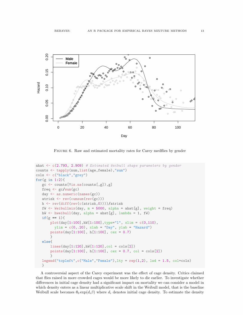
Data from this experiment is available from the REBayes with further details documented there.All three of the principle conclusions of the study are illustrated in Figure 6. As specified in

the code fragment below we compute daily death counts by age and gender, allowing us to plotraw mortality rates by gender. We then estimate the Weibull mixture model using gender specificWeibull shape parameters as described in Koenker and Gu (2013). As illustrated in the displayedcode, given the estimated mixing distribution it is easy to compute the hazard functions of thecorresponding mixture distributions.

data(flies)

attach(flies)

hweibull <- function(s,alpha,lambda, f){

Lambda<-outer((lambda*s)^(alpha),exp(f$x))

Surv <- exp(-Lambda) %*% f$y/sum(f$y)

A <- matrix(0, length(s), length(f$x))

for (i in 1:length(s)){

for (j in 1:length(f$x))

A[i,j] <- dweibull(s[i],shape=alpha,

scale = lambda^(-1) * (exp(f$x[j]))^(-1/alpha))

}

g <- A %*% f$y

g/(sum(g)*Surv)

}


0 20 40 60 80 100

0.00

0.05

0.10

0.15

0.20

Day

Haz

ard

●●●●●●●

●●

●●●

●●

●●

●

●●

●

●●

●

●

●

●

●●●

●●●

●●●

●

●

●

●●

●●

●●

●●

●

●

●

●

●

●●

●

●●

●●

●

●

●

●

●

●

●

●●

●

●

●

●

●

●●

●

●

●

●

●

●

●

●

●

●●

●

●

●

●

●

●●

●●

●●

MaleFemale

●●●●●●

●●

●

●

●

●

●

●

●●●●●

●●●●●●

●●

●

●●

●

●●●

●●

●

●

●●●●

●

●

●

●

●●

●

●

●

●

●

●

●●

●

●●

●●

●

●

●

●

●

●

●

●

●

●

●

●

●

●●

●

●

●

●

●

●

●

●●

●

●

●

●

●

●

●

●

●

●●

●

●

●

●

MaleFemale

Figure 6. Raw and estimated mortality rates for Carey medflies by gender

ahat <- c(2.793, 2.909) # Estimated Weibull shape parameters by gender

counts <- tapply(num,list(age,female),"sum")

cols <- c("black","grey")

for(g in 1:2){

gc <- counts[!is.na(counts[,g]),g]

freq <- gc/sum(gc)

day <- as.numeric(names(gc))

atrisk <- rev(cumsum(rev(gc)))

h <- rev(diff(rev(c(atrisk,0))))/atrisk

fW <- Weibullmix(day, m = 5000, alpha = ahat[g], weight = freq)

hW <- hweibull(day, alpha = ahat[g], lambda = 1, fW)

if(g == 1){

plot(day[1:100],hW[1:100],type="l", xlim = c(0,110),

ylim = c(0,.20), xlab = "Day", ylab = "Hazard")

points(day[1:100], h[1:100], cex = 0.7)

}

else{

lines(day[1:120],hW[1:120],col = cols[2])

points(day[1:100], h[1:100], cex = 0.7, col = cols[2])

}

legend("topleft",c("Male","Female"),lty = rep(1,2), lwd = 1.5, col=cols)

}

A controversial aspect of the Carey experiment was the effect of cage density. Critics claimedthat flies raised in more crowded cages would be more likely to die earlier. To investigate whetherdifferences in initial cage density had a significant impact on mortality we can consider a model inwhich density enters as a linear multiplicative scale shift in the Weibull model, that is the baselineWeibull scale becomes θ0 exp(diβ) where di denotes initial cage density. To estimate the density


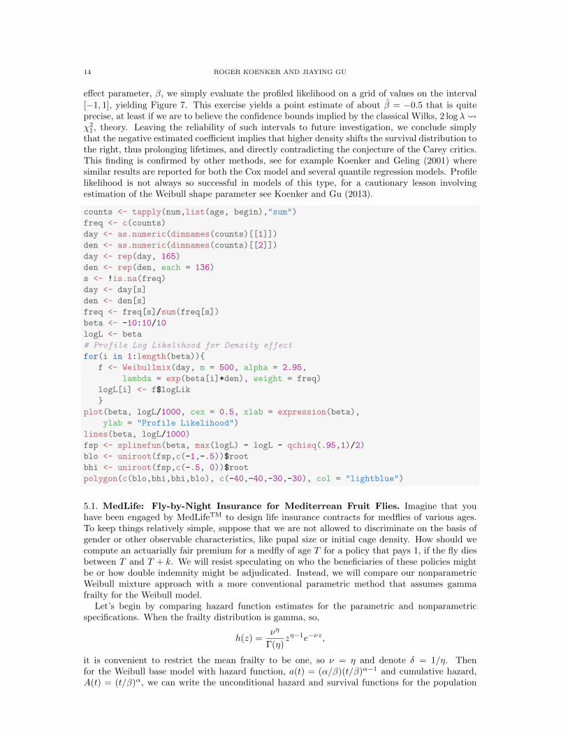
effect parameter, β, we simply evaluate the profiled likelihood on a grid of values on the interval

[−1, 1], yielding Figure 7. This exercise yields a point estimate of about β = −0.5 that is quiteprecise, at least if we are to believe the confidence bounds implied by the classical Wilks, 2 log λ χ21, theory. Leaving the reliability of such intervals to future investigation, we conclude simply

that the negative estimated coefficient implies that higher density shifts the survival distribution tothe right, thus prolonging lifetimes, and directly contradicting the conjecture of the Carey critics.This finding is confirmed by other methods, see for example Koenker and Geling (2001) wheresimilar results are reported for both the Cox model and several quantile regression models. Profilelikelihood is not always so successful in models of this type, for a cautionary lesson involvingestimation of the Weibull shape parameter see Koenker and Gu (2013).

counts <- tapply(num,list(age, begin),"sum")

freq <- c(counts)

day <- as.numeric(dimnames(counts)[[1]])

den <- as.numeric(dimnames(counts)[[2]])

day <- rep(day, 165)

den <- rep(den, each = 136)

s <- !is.na(freq)

day <- day[s]

den <- den[s]

freq <- freq[s]/sum(freq[s])

beta <- -10:10/10

logL <- beta

# Profile Log Likelihood for Density effect

for(i in 1:length(beta)){

f <- Weibullmix(day, m = 500, alpha = 2.95,

lambda = exp(beta[i]*den), weight = freq)

logL[i] <- f$logLik

}

plot(beta, logL/1000, cex = 0.5, xlab = expression(beta),

ylab = "Profile Likelihood")

lines(beta, logL/1000)

fsp <- splinefun(beta, max(logL) - logL - qchisq(.95,1)/2)

blo <- uniroot(fsp,c(-1,-.5))$root

bhi <- uniroot(fsp,c(-.5, 0))$root

polygon(c(blo,bhi,bhi,blo), c(-40,-40,-30,-30), col = "lightblue")

5.1. MedLife: Fly-by-Night Insurance for Mediterrean Fruit Flies. Imagine that youhave been engaged by MedLifeTM to design life insurance contracts for medflies of various ages.To keep things relatively simple, suppose that we are not allowed to discriminate on the basis ofgender or other observable characteristics, like pupal size or initial cage density. How should wecompute an actuarially fair premium for a medfly of age T for a policy that pays 1, if the fly diesbetween T and T + k. We will resist speculating on who the beneficiaries of these policies mightbe or how double indemnity might be adjudicated. Instead, we will compare our nonparametricWeibull mixture approach with a more conventional parametric method that assumes gammafrailty for the Weibull model.

Let’s begin by comparing hazard function estimates for the parametric and nonparametricspecifications. When the frailty distribution is gamma, so,

h(z) =νη

Γ(η)zη−1e−νz,

it is convenient to restrict the mean frailty to be one, so ν = η and denote δ = 1/η. Thenfor the Weibull base model with hazard function, a(t) = (α/β)(t/β)α−1 and cumulative hazard,A(t) = (t/β)α, we can write the unconditional hazard and survival functions for the population


●

●

●●

● ● ●●

●

●

●

●

●

●

●

●

●

●

●

●

●

−1.0 −0.5 0.0 0.5 1.0

−37

.4−

37.0

−36

.6

β

Pro

file

Like

lihoo

d

Figure 7. Initial Cage Density Effect in the Weibull Mixture Model: Profile LogLikelihood (in 1000’s) for the cage density effect with 0.95 (Wilks) confidenceinterval in blue.

as,λ(t) = a(t)/(1 + δA(t))

andS(t) = (1 + δA(t))−1/δ.

This yields the loglikelihood,

`(α, β, δ|t) =

n∑i=1

log a(ti)− (1 + 1/δ) log(1 + δA(ti)).

GammaFrailty <- function(pars, age, num, hazard = FALSE){

alpha <- pars[1]

beta <- pars[2]

delta <- pars[3]

a <- (alpha/beta) * (age/beta)^(alpha - 1) # Weibull hazard

A <- (age/beta)^alpha # Weibull cumulative hazard

if(hazard)

z <- a/(1 + delta * A)

else

z <- -sum(num * (log(a) - (1 + 1/delta)* log(1 + delta * A)))

z

}

pars <- c(5, 20, 1) # Initial values

z <- optim(pars, GammaFrailty, age = age, num = num)

fitG <- z$par

fitW <- Weibullmix(day, m = 5000, alpha = 2.95, weights = freq)


●●●●●●

●●

●

●

●

●

●

●●

●●

●●

●

●●

●

●●

●

●●

●

●

●●●

●●●●

●

●

●●

●●

●

●

●

●

●

●

●

●

●

●●

●

●●●

●

●

●●

●

●

●

●

●

●

●

●

●

●●

●

●

●

●

●

●

●●

●

●●

●●

●

●

●

●

●

●

●

●

●

●●

●

●

●

●

● ●●●

●●●●

●

0 20 40 60 80 100 120

0.00

0.05

0.10

0.15

day

haza

rd

NPMLEGamma

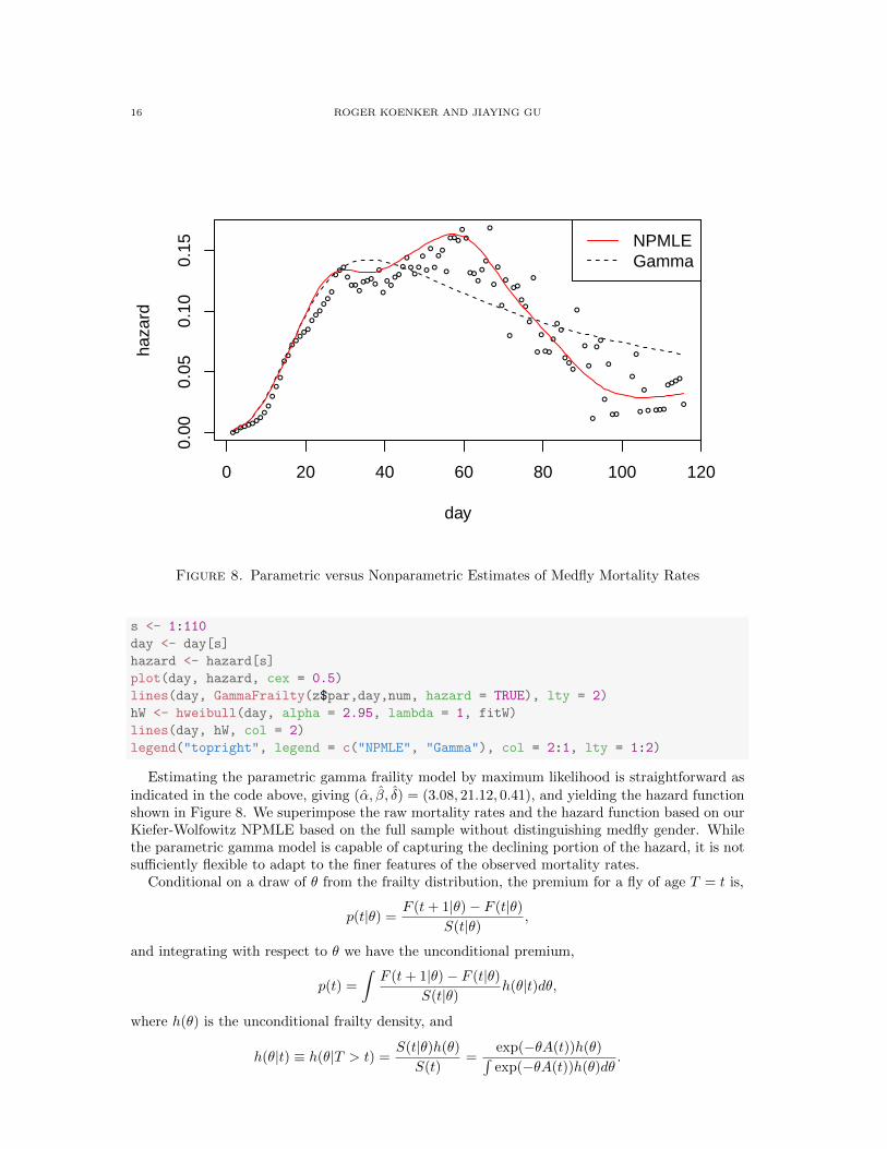
Figure 8. Parametric versus Nonparametric Estimates of Medfly Mortality Rates

s <- 1:110

day <- day[s]

hazard <- hazard[s]

plot(day, hazard, cex = 0.5)

lines(day, GammaFrailty(z$par,day,num, hazard = TRUE), lty = 2)

hW <- hweibull(day, alpha = 2.95, lambda = 1, fitW)

lines(day, hW, col = 2)

legend("topright", legend = c("NPMLE", "Gamma"), col = 2:1, lty = 1:2)

Estimating the parametric gamma fraility model by maximum likelihood is straightforward as

indicated in the code above, giving (α, β, δ) = (3.08, 21.12, 0.41), and yielding the hazard functionshown in Figure 8. We superimpose the raw mortality rates and the hazard function based on ourKiefer-Wolfowitz NPMLE based on the full sample without distinguishing medfly gender. Whilethe parametric gamma model is capable of capturing the declining portion of the hazard, it is notsufficiently flexible to adapt to the finer features of the observed mortality rates.

Conditional on a draw of θ from the frailty distribution, the premium for a fly of age T = t is,

p(t|θ) =F (t+ 1|θ)− F (t|θ)

S(t|θ),

and integrating with respect to θ we have the unconditional premium,

p(t) =

∫F (t+ 1|θ)− F (t|θ)

S(t|θ)h(θ|t)dθ,

where h(θ) is the unconditional frailty density, and

h(θ|t) ≡ h(θ|T > t) =S(t|θ)h(θ)

S(t)=

exp(−θA(t))h(θ)∫exp(−θA(t))h(θ)dθ

.


is the corresponding conditional frailty density. The need to condition the frailty distribution ont may seem odd, but a moment’s reflection reveals that mass associated with high frailty valuesthat would imply that subjects would die very quickly, must surely be downweighted once subjectsattain an age at which having these values is highly improbable. This is illustrated in Figure 9where we depict the estimated, conditional frailty based on our NPMLE at four different ages.To exaggerate the magnitude of the smaller mass points of the NPMLE we have plotted the cuberoot of the density. It is clear that the relatively small mass point at log(θ) = −3.4 at age 1.5, byage 20 is no longer visible; flies with such a large frailty would almost surely be dead by age 20.

Gfrailt <- function(age, fit){

alpha <- fit[1]

beta <- fit[2]

delta <- fit[3]

A <- (age/beta)âlpha # Weibull cumulative hazard

(1 + delta * A)^(-1/delta)

}

frailt <- function(v, t, alpha, fit){

fv = fit$y/sum(fit$y)

g = sum(exp(-v * (tâlpha))* fv)

exp(-v * (tâlpha)) * fv/g

}

par(mfrow = c(2,2))

v <- exp(fitW$x)

for(t in c(1.5, 20, 60, 100)){

plot(log(v), frailt(v, t, alpha = 2.95, fitW)^(1/3), type="l",

main = paste("age =", t),

xlab = expression(log(theta)),

ylab = expression(h( theta , t)^{1/3}))

}

In Figure 10 we plot the ten-day term life insurance premium for medflies at various ages forboth the parametric gamma model and the nonparametric model. By varying the parameter k inthe premium function one can control the term of the life insurance policy. In the figure k = 10and the premia profile is somewhat smoother than the instantaneous hazard depicted in Figure 8.Again we see that the gamma model captures the basic shape of the nonparametric rate structure,but misses some of the nuances.

premium <- function(v, t, k = 1, alpha, fit){

if("Weibullmix" %in% class(fit)) {

R <- t

for(i in 1:length(t)){

D <- exp(-v * t[i]âlpha) - exp(-v * (t[i] + k)âlpha)

D <- D/exp(-v * t[i]âlpha)

D[is.nan(D)] <- 1 # Kludge for vampire medflies

R[i] <- sum(D * frailt(v, t[i], alpha, fit))

}

}

else

R <- (Gfrailt(t,fit) - Gfrailt(t+k, fit))/Gfrailt(t, fit)

R

}

v <- exp(fitW$x)

R <- premium(v, day, k = 10, alpha = 2.95, fitW)

plot(day, R, type = "l", col = 2, ylab = "Premium")

R <- premium(v, day, k = 10, alpha = 2.95, fitG)


−14 −12 −10 −8 −6 −4 −2

0.0

0.2

0.4

0.6

0.8

age = 1.5

log(θ)

h(θ,

t)1

3

−14 −12 −10 −8 −6 −4 −2

0.0

0.2

0.4

0.6

age = 20

log(θ)

h(θ,

t)1

3

−14 −12 −10 −8 −6 −4 −2

0.0

0.2

0.4

0.6

0.8

age = 60

log(θ)

h(θ,

t)1

3

−14 −12 −10 −8 −6 −4 −2

0.0

0.2

0.4

0.6

0.8

1.0

age = 100

log(θ)

h(θ,

t)1

3

Figure 9. Conditional Frailty at Various Ages: Note that the cube root of thefrailties have been plotted to accentuate the smaller mass points

lines(day, R, lty = 2)

legend("topright", legend = c("NPMLE", "Gamma"), col = 2:1, lty = 1:2)

6. Conclusion

We have described a new approach to computing the nonparametric maximum likelihood es-timator of Kiefer and Wolfowitz for a general class of mixture models as implemented in theR package REBayes, and illustrated its application in a variety mixture model settings. Theapproach exploits recent developments in convex optimization as implemented in the Mosek en-vironment of Andersen (2010). Koenker and Mizera (2014a) surveys a broader range of suchdevelopments. In addition to the capabilities intended for mixture models the REBayes packagecontains the function medde for norm and shape constrained density estimation. Further details onmedde methods may be found in Koenker and Mizera (2010) and the REBayes documentation.


0 20 40 60 80 100 120

0.2

0.4

0.6

0.8

day

Pre

miu

m

NPMLEGamma

Figure 10. Ten-Day Term Life Insurance Premia for Medflies of Various Ages

References

Aalen O, Borgan O, Gjessing H. 2008. Survival and Event History Analysis. Springer.Andersen ED. 2010. The Mosek optimization tools manual, version 6.0. Available fromhttp://www.mosek.com.

Brown L. 2008. In-season prediction of batting averages: A field test of empirical Bayes and Bayesmethodologies. The Annals of Applied Statistics 2: 113–152.

Brown L, Greenshtein E. 2009. Non parametric empirical Bayes and compound decision approachesto estimation of a high dimensional vector of normal means. The Annals of Statistics 37: 1685–1704.

Buhlmann H, Gisler A. 2005. A Course in Credibility Theory and its Applications. Springer.Carey J, Liedo P, Orozco D, Vaupel J. 1992. Slowing of mortality rates at older ages in large

medfly cohorts. Science 258: 457–61.Castillo I, van der Vaart A. 2012. Needles and straw in a haystack: Posterior concentration for

possibly sparse sequences. Annals of Statistics 40: 2069–2101.Dicker L, Zhao SD. 2014. Nonparametric empirical Bayes and maximum likelihood estimation for

high-dimensional data analysis. Available from arxiv.org/pdf/1407.2635.Dyson F. 1926. A method for correcting series of parallax observations. Monthly Notices of the

Royal Astronomical Society 86: 686–706.Efron B. 2008. Simultaneous inference: When should hypothesis testing problems be combined?

The Annals of Applied Statistics 2: 197–223.Efron B. 2010. Large-Scale Inference: Empirical Bayes Methods for Estimation, Testing, and

Prediction. Cambridge U. Press: Cambridge.Efron B. 2011. Tweedie’s formula and selection bias. Journal of the American Statistical Associ-

ation 106: 1602–1614.Friberg HA. 2012. Users guide to the R-to-Mosek interface. Available from http://rmosek.

r-forge.r-project.org.

arxiv.org/pdf/1407.2635

http://rmosek.r-forge.r-project.org

http://rmosek.r-forge.r-project.org


Gu J, Koenker R. 2015a. Empirical Bayesball remixed: Empirical Bayes methods for longitudinaldata. Preprint.

Gu J, Koenker R. 2015b. On a problem of Robbins. International Statistical Review Forthcoming.Gu J, Koenker R. 2015c. Unobserved heterogeneity in income dynamics: An empirical Bayes

perspective. J. of Economic and Business Statistics Forthcoming.Haastrup S. 2000. Comparison of some Bayesian analyses of heterogeneity in group life insurance.

Scand. Actuarial J. : 2–16.Heckman J, Singer B. 1984. A method for minimizing the impact of distributional assumptions in

econometric models for duration data. Econometrica 52: 63–132.Jiang W, Zhang CH. 2009. General maximum likelihood empirical Bayes estimation of normal

means. Annals of Statistics 37: 1647–1684.Jiang W, Zhang CH. 2015. Generalized likelihood ratio test for normal mixtures. Statistica Sinica

Forthcoming.Johnstone I, Silverman B. 2004. Needles and straw in haystacks: Empirical Bayes estimates of

possibly sparse sequences. Annals of Statistics : 1594–1649.Kiefer J, Wolfowitz J. 1956. Consistency of the maximum likelihood estimator in the presence of

infinitely many incidental parameters. The Annals of Mathematical Statistics 27: 887–906.Koenker R. 2013. Adaptive estimation of regression parameters for the Gaussian scale mixture

model. In Beran J, Feng Y, Hebbel H (eds.) Empirical Economic and Financial Research: AFestschrift for Siegfried Heiler. Springer, 373–378.

Koenker R. 2014. A Gaussian compound decision bakeoff. Stat 3: 12–16.Koenker R, Geling O. 2001. Reappraising medfly longevity: A quantile regression survival analysis.

J. of Am. Stat. Assoc. 96: 458–468.Koenker R, Gu J. 2013. Frailty, profile likelihood and medfly mortality. In Lahiri S, Schick A,

Sengupta A, Sriram T (eds.) Contemporary Developments in Statistical Theory: A Festschriftfor Hira Lal Koul. Springer.

Koenker R, Mizera I. 2010. Quasi-concave density estimation. The Annals of Statistics 38: 2998–3027.

Koenker R, Mizera I. 2014a. Convex optimization in R. Journal of Statistical Software 60.Koenker R, Mizera I. 2014b. Convex optimization, shape constraints, compound decisions and

empirical Bayes rules. J. of Am. Stat. Assoc. 109: 674–685.Laird N. 1978. Nonparametric maximum likelihood estimation of a mixing distribution. Journal

of the American Statistical Association 73: 805–811.Lindsay B. 1983. The geometry of mixture likelihoods: A general theory. Annals of Statistics 11:

86–94.Martin R, Walker SG. 2013. Asymptotically minimax empirical Bayes estimation of a sparse

normal mean. arXiv:1304.7366 .Norberg R. 1989. Experience rating in group life insurance. Scand. Actuarial J. : 194–224.Pearson K. 1894. Contributions to the mathematical theory of evolution. Phil. Trans. Roy. Soc.

London A 185: 71–110.Robbins H. 1950. A generalization of the method of maximum likelihood; estimating a mixing

distribution (preliminary report). Annals of Mathematical Statistics 21: 314–315.Robbins H. 1951. Asymptotically subminimax solutions of compound statistical decision problems.

In Proceedings of the Berkeley Symposium on Mathematical Statistics and Probability, volume I.University of California Press: Berkeley, 131–149.

Robbins H. 1956. An empirical Bayes approach to statistics. In Proceedings of the Third BerkeleySymposium on Mathematical Statistics and Probability, volume I. University of California Press:Berkeley, 157–163.

Sun W, Cai TT. 2007. Oracle and adaptive compound decision rules for false discovery ratecontrol. J. American Statistical Association 102: 901–912.

Sun W, McLain AC. 2012. Multiple testing of composite null hypotheses in heteroscedastic models.Journal of the American Statistical Association 107: 673–687.

Teicher H. 1967. Identifiability of mixtures of product measures. Annals of Mathematical Statistics38: 1300–1302.


Vaupel J, Manton K, Stollard E. 1979. The impact of heterogeneity in individual frailty on thedynamics of mortality. Demography 16: 439–454.

Rebayes: an R package for empirical bayes mixture methods

Documents

Transcript of Rebayes: an R package for empirical bayes mixture methods