
Reasoning about High-Level Constructs in · PDF filePermission to make digital or hard copies...
117
Reasoning about High-Level Constructs in Hardware/Software Formal Verification Jiang Long Electrical Engineering and Computer Sciences University of California at Berkeley Technical Report No. UCB/EECS-2017-150 http://www2.eecs.berkeley.edu/Pubs/TechRpts/2017/EECS-2017-150.html August 14, 2017
Transcript of Reasoning about High-Level Constructs in · PDF filePermission to make digital or hard copies...

Reasoning about High-Level Constructs inHardware/Software Formal Verification
Jiang Long
Electrical Engineering and Computer SciencesUniversity of California at Berkeley
Technical Report No. UCB/EECS-2017-150http://www2.eecs.berkeley.edu/Pubs/TechRpts/2017/EECS-2017-150.html
August 14, 2017

Copyright © 2017, by the author(s).All rights reserved.
Permission to make digital or hard copies of all or part of this work forpersonal or classroom use is granted without fee provided that copies arenot made or distributed for profit or commercial advantage and that copiesbear this notice and the full citation on the first page. To copy otherwise, torepublish, to post on servers or to redistribute to lists, requires prior specificpermission.
Acknowledgement
I like to thank Prof. Robert K. Brayton for accepting me into his PhDprogram in Fall 2008. I remembered his Phil Kaulfman award ceremony atDAC 2008, where he concluded this speech by answering a question fromthe audience on what is his secrets in advising students:Leave them alone, don’t mess them up, give a hand when they are in need ofa help.At times, I was indeed left alone, given space(maybe too much) to exploremy interest, stretch my ability and forge forward on my own, but obtaininghis guidance and support at times of doubt and breaking point which carriedme through the PhD journey. I would not start nor reach the finishing pointwithout Bob’s support or guidance.I ike to thank Dr. Alan Mishchencko for introducing me to Bob’s researchgroup in the first place.

Reasoning about High-Level Constructs in Hardware/Software FormalVerification
by
Jiang Long
A dissertation submitted in partial satisfaction of the
requirements for the degree of
Doctor of Philosophy in Engineering
–
Electrical Engineering and Computer Science
in the
Graduate Division
of the
University of California, Berkeley
Committee in charge:
Professor Robert K. Brayton, ChairProfessor Alberto Sangiovanni Vincentelli
Professor Xinyi Yuan
Summer 2017

Reasoning about High-Level Constructs in Hardware/Software Formal
Verification
Copyright 2017
by
Jiang Long

1
Abstract
Reasoning about High-Level Constructs in Hardware/Software Formal Verification
by
Jiang Long
Doctor of Philosophy in Engineering in Electrical Engineering and Computer Science
University of California, Berkeley
Professor Robert K. Brayton, Chair
The ever shrinking feature size of modern electronic chips leads to more designs being done
as well as more complex chips being designed. These in turn lead to greater use of high-level
specifications and to more sophisticated optimizations applied at the word -level. These steps
make it more difficult to verify that the final design is faithful to the initial specification.
We tackle two steps in this process and their formal equivalence checking to help verify the
correctness of the steps.
First, we present LEC, a combinational equivalence checking tool that is learning driven.
It focuses on data-path equivalence checking with the goal of transforming the two logics
under comparison to be more similar in order to reduce the complexity of a final Boolean
(bit-level) solving. LEC does equivalence checking of combinational logic between two RTL
(word-level) designs, one the original and one an optimized RTL version. LEC features an
open architecture such that users and developers can learn with the system as new designs
and optimizations are met, and then it can be modularly extended with new proof procedures
as they are discovered.
To address the use of higher level specifications, we build a simple trusted C to Verilog trans-
lation procedure based on the LLVM compiler infrastructure. The translator was designed to
implement an almost vertatim translation of the C language operators and control structures

2
into the Verilog always ff and always comb blocks through traversing LLVM Bytecode pro-
grams. The procedure reliably bridges the language barrier between software and hardware
and allows hardware synthesis and verification techniques to be applied readily.
In combination, these two procedures allow for equivalence checking between a software-like
specification and an optimized word-level RTL implementation.

i
Contents
Contents i
List of Figures v
List of Tables vii
1 Introduction 11.1 Motivation . . . . . . . . . . . . . . . . . . . . . . . . . . . . . . . . . . . . . 11.2 Thesis Contribution . . . . . . . . . . . . . . . . . . . . . . . . . . . . . . . . 3
2 Data-path Design Space and Verification 42.1 Introduction . . . . . . . . . . . . . . . . . . . . . . . . . . . . . . . . . . . . 52.2 Data-path Optimization: The Design Space . . . . . . . . . . . . . . . . . . 62.3 About Adding a Set of Numbers . . . . . . . . . . . . . . . . . . . . . . . . . 102.4 Empirical Study: Eight-Operand Adder-Tree Equivalence Checking . . . . . 112.5 Survey: Data-Path Formal Verification Techniques . . . . . . . . . . . . . . . 15
3 LEC: Learning-Driven Equivalence Checking 293.1 Overview: A Learning Process - Philosophy . . . . . . . . . . . . . . . . . . 293.2 Tool Flow and Organization . . . . . . . . . . . . . . . . . . . . . . . . . . . 313.3 The LEC Widgets . . . . . . . . . . . . . . . . . . . . . . . . . . . . . . . . . 333.4 System Integration: Proof-tree Infrastructure . . . . . . . . . . . . . . . . . . 533.5 Case Studies . . . . . . . . . . . . . . . . . . . . . . . . . . . . . . . . . . . . 563.6 Experimental Results . . . . . . . . . . . . . . . . . . . . . . . . . . . . . . . 613.7 Comparison with Related Work . . . . . . . . . . . . . . . . . . . . . . . . . 653.8 Conclusion . . . . . . . . . . . . . . . . . . . . . . . . . . . . . . . . . . . . . 67
4 A Simple Trusted Translation Procedure from C to Verilog 684.1 Introduction . . . . . . . . . . . . . . . . . . . . . . . . . . . . . . . . . . . . 694.2 Background . . . . . . . . . . . . . . . . . . . . . . . . . . . . . . . . . . . . 744.3 Translating SSA to Verilog . . . . . . . . . . . . . . . . . . . . . . . . . . . . 814.4 Experiments . . . . . . . . . . . . . . . . . . . . . . . . . . . . . . . . . . . . 904.5 Related works . . . . . . . . . . . . . . . . . . . . . . . . . . . . . . . . . . . 95

ii
4.6 Conclusions . . . . . . . . . . . . . . . . . . . . . . . . . . . . . . . . . . . . 96
5 Conclusion and Possible Future Extensions 97
Bibliography 99

iii
Acknowledgments
First and foremost, I would like to thank my advisor Prof. Robert K. Brayton for accepting
me into his PhD program in Fall 2008. I remembered his Phil Kaulfman award ceremony at
DAC 2008, where he concluded this award speech by answering a question from the audience
on what is his secrets in advising his students:
Leave them alone, don’t mess them up, give a hand when they are in need of a
help.
At times, I was indeed left alone, given space(maybe too much) to explore my interest,
stretch my ability and forge forward on my own, but obtaining his guidance and support at
times of doubt and breaking point which carried me through the PhD journey. I would not
start nor reach the finishing point without Bob’s support or guidance.
I would also like to thank Dr. Alan Mishchencko for introducing me to Bob’s research
group in the first place. His enthusiasm, deep devotion and extertise to the design and
implementation of ABC not only provides us with a research foundation but also bring us
closer to the industry for accessing real practical problems. In that, I would like to thank
Dr. Mike Case for sharing an interesting problem with our research group which led to the
starting point of this thesis work in data-path equivalence checking.
I am thankful to my Qual exam committee members, Prof. Sanjit Seisha, Prof. Andreas
Kuehlmann, and Prof. Xinyi Yuan for overseeing the exam.
The thesis work is built upon Verific Inc.’s HDL compiler frontends, without them, it would
not be possible. Personally, I would like to thank Baruch Sterin, Niklas Een, Yen-sheng Ho,
Yu-yun Dai for the invigorating group discussions and introducing me to Python, bitbucket,
hg and many other new tools which are the building blocks in the thesis implementation.

iv
吾生也有涯,
而知也无涯。
以有涯随无涯,
殆已;
已而为知者,
殆而已矣。
庄子 (300. BC)
Life has its bound,
Thou learning does not.
With the bounded to follow the unbounded,
Trying thee;
Knowningly pursue the unknown,
Trying trying thee.
Zhuang Zi (300. BC)

v
List of Figures
1.1 Design Abstraction Levels . . . . . . . . . . . . . . . . . . . . . . . . . . . . . . 2
2.1 A×B = Sum of n2 partial products . . . . . . . . . . . . . . . . . . . . . . . . 112.2 Linear Adder Tree described in Verilog . . . . . . . . . . . . . . . . . . . . . . . 122.3 adder tree structure. . . . . . . . . . . . . . . . . . . . . . . . . . . . . . . . . . 132.4 ABC’s dcec results . . . . . . . . . . . . . . . . . . . . . . . . . . . . . . . . . . 142.5 Complexity scale of SAT-Sweeping . . . . . . . . . . . . . . . . . . . . . . . . . 142.6 Bit-level to word-level transformation . . . . . . . . . . . . . . . . . . . . . . . . 152.7 Use of UIF . . . . . . . . . . . . . . . . . . . . . . . . . . . . . . . . . . . . . . 17
3.1 Miter logic . . . . . . . . . . . . . . . . . . . . . . . . . . . . . . . . . . . . . . . 303.2 Overall tool flow . . . . . . . . . . . . . . . . . . . . . . . . . . . . . . . . . . . 323.3 Illustration WNK node in C++ class . . . . . . . . . . . . . . . . . . . . . . . . 323.4 Proof process . . . . . . . . . . . . . . . . . . . . . . . . . . . . . . . . . . . . . 343.5 Model Tree from Structural Hashing Widget . . . . . . . . . . . . . . . . . . . . 373.6 Model Tree from Constant Reduction Widget . . . . . . . . . . . . . . . . . . . 383.7 Model Tree from PEP Reduction Widget . . . . . . . . . . . . . . . . . . . . . . 393.8 Model Tree from the Abstraction Widget . . . . . . . . . . . . . . . . . . . . . . 393.9 Case-split Transformation Widget . . . . . . . . . . . . . . . . . . . . . . . . . . 433.10 Algebraic Transformations . . . . . . . . . . . . . . . . . . . . . . . . . . . . . . 433.11 Algebraic transformation Widget . . . . . . . . . . . . . . . . . . . . . . . . . . 443.12 Miter network . . . . . . . . . . . . . . . . . . . . . . . . . . . . . . . . . . . . . 463.13 Constant Learning and Reduction Widgets . . . . . . . . . . . . . . . . . . . . . 483.14 PEP Learning and Reduction Widgets . . . . . . . . . . . . . . . . . . . . . . . 493.15 Annotated reduced graph . . . . . . . . . . . . . . . . . . . . . . . . . . . . . . 523.16 Branching sub-model tree . . . . . . . . . . . . . . . . . . . . . . . . . . . . . . 543.17 Illustration of proof log . . . . . . . . . . . . . . . . . . . . . . . . . . . . . . . . 553.18 Sub-model proof tree . . . . . . . . . . . . . . . . . . . . . . . . . . . . . . . . 573.19 Addition implementation . . . . . . . . . . . . . . . . . . . . . . . . . . . . . . . 593.20 Proof log . . . . . . . . . . . . . . . . . . . . . . . . . . . . . . . . . . . . . . . 60

vi
3.21 WNK network for adder-shift tree of lemma 64 (Figure 3.20 line 26, equation(3.33) ) ( pi, po. +,{},[m:n] are input, output, full-adder, concat and extractoperators. The number after ’ ’ is the bit-width of the node. ) . . . . . . . . . 62
4.1 C vs RTL equivalence checking . . . . . . . . . . . . . . . . . . . . . . . . . . . 704.2 sum02 true-unreach-call.c . . . . . . . . . . . . . . . . . . . . . . . . . . . . . . 714.3 C-to-Verilog Translation . . . . . . . . . . . . . . . . . . . . . . . . . . . . . . . 734.4 A single-clock synchronous circuit . . . . . . . . . . . . . . . . . . . . . . . . . . 744.5 Verilog factorial implementation . . . . . . . . . . . . . . . . . . . . . . . . . . . 764.6 Waveform for Module verilog factorialwithn = 6 . . . . . . . . . . . . . . . . . 774.7 C to SSA IR illustration . . . . . . . . . . . . . . . . . . . . . . . . . . . . . . . 784.8 LLVM CFG . . . . . . . . . . . . . . . . . . . . . . . . . . . . . . . . . . . . . 804.9 SSAb from SSA in Figure 4.7c with phi node reverted . . . . . . . . . . . . . . . 824.10 Verilog Model . . . . . . . . . . . . . . . . . . . . . . . . . . . . . . . . . . . . . 834.11 SSA access and utility functions . . . . . . . . . . . . . . . . . . . . . . . . . . . 864.12 SSAb to Verilog Translation . . . . . . . . . . . . . . . . . . . . . . . . . . . . . 874.13 Translation to Verilog continued . . . . . . . . . . . . . . . . . . . . . . . . . . . 884.14 Translated Verilog module from the SSAb in Figure 4.9 . . . . . . . . . . . . . 894.15 Waveform for Verilog module factorial . . . . . . . . . . . . . . . . . . . . . . . 904.16 test:bitvector-loops/overflow false-unreach-call1.i . . . . . . . . . . . . . . . . . . 934.17 Software Verification Benchmark: bitvector category . . . . . . . . . . . . . . . 94

vii
List of Tables
2.1 Result of three data-path transformations . . . . . . . . . . . . . . . . . . . . . 102.2 Internal similarities between Adder Trees in Figure 2.3 . . . . . . . . . . . . . . 132.3 ACL2 Axioms . . . . . . . . . . . . . . . . . . . . . . . . . . . . . . . . . . . . . 22
3.1 Supported operators (unsigned) . . . . . . . . . . . . . . . . . . . . . . . . . . . 323.2 Lemma Types(MM is the current model) . . . . . . . . . . . . . . . . . . . . . . 353.3 Rewriting rules . . . . . . . . . . . . . . . . . . . . . . . . . . . . . . . . . . . . 403.4 Rewriting Widget . . . . . . . . . . . . . . . . . . . . . . . . . . . . . . . . . . . 413.5 Disjunctions of s-lemmas . . . . . . . . . . . . . . . . . . . . . . . . . . . . . . . 543.6 Conjunction of e-lemmas . . . . . . . . . . . . . . . . . . . . . . . . . . . . . . . 543.7 Benchmark comparison (Timeout 24 hours) . . . . . . . . . . . . . . . . . . . . 63
4.1 2015 Software Verification Competition: Bit-Vector category . . . . . . . . . . . 724.2 Verilog language elements . . . . . . . . . . . . . . . . . . . . . . . . . . . . . . 754.3 C language elements . . . . . . . . . . . . . . . . . . . . . . . . . . . . . . . . . 764.4 fpu 100 : 32-bit FPU . . . . . . . . . . . . . . . . . . . . . . . . . . . . . . . . . 914.5 fpu double: 64-bit FPU . . . . . . . . . . . . . . . . . . . . . . . . . . . . . . . 92
1
Chapter 1
Introduction
One of the driving force of
high-level language constructs
is the need to raise the
abstraction level for
productivity.
1.1 Motivation
The technological driving force of the chip-design industry is the feature width in the semi-
conductor device fabrication process, which reduces from 10µm in 1971 to 10nm in 2016. As
of 2014, leading SoC (System-on-Chip) designs, such as Apple A8 chip, contains over two
billion transistors on a 89mm2 piece of silicon. Ignoring the manufacturing aspect of the chip
production process, just focusing on the functions these chips implement, the sheer task of
assembling two billion transistors together is a daunting one for human minds to attain. To
achieve this, programming languages are relied on to design the functionality and compiler
and synthesis technologies are used to generate the circuit.
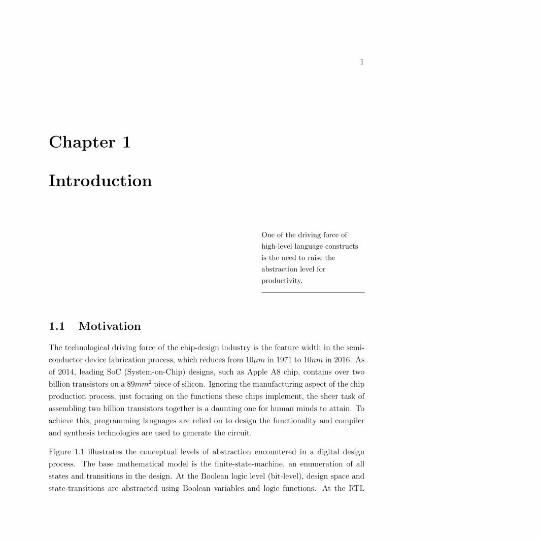
Figure 1.1 illustrates the conceptual levels of abstraction encountered in a digital design
process. The base mathematical model is the finite-state-machine, an enumeration of all
states and transitions in the design. At the Boolean logic level (bit-level), design space and
state-transitions are abstracted using Boolean variables and logic functions. At the RTL

CHAPTER 1. INTRODUCTION 2
C/C++/SystemC Software Model
Verilog/VHDL RTL Design
Boolean Logic Circuit
Finite State Machine (FSM)
Figure 1.1: Design Abstraction Levels
level (word-level), the design functionalities are described using programming language con-
structs and the underlying mathematical model is bit-vector or integer arithmetic. High-level
languages provide syntax and semantics for hierarchical and modular design methodologies,
which makes it possible to build a chip with billions of transistors.
Hardware design languages, like Verilog or VHDL, have syntactical constructs for clocks,
flops, logical gates, bit-vectors, etc. They statically allocate memory and computation re-
sources which corresponds directly to the physical elements in the circuits. On the other
hand, software based design languages do not have a clocking concept nor basic logic gates
explicitly, but have constructs for integers, while/for loops, dynamic memory allocation,
run-time function calls, and threads, etc. This expedites design productivity by describing
the functionality through more powerful and expressive programming constructs. In indus-
trial practice, software based languages have been used for prototyping, creating reference
models and performance models. These are built in advance and maintained as the RTL
design process progresses. In Colwell’s “Pentium Chronicles” book[20], the idea for out-of-
order pipelined micro-code instruction execution was first validated on VAX’s instruction
sequences using a software model. During Pentium’s design creation at Intel, a behavior
model in C was created first and maintained rigorously throughout the design process. The
author attributed the use of a C-model as a crucial element in Pentium’s product success.
As the design functionality is more frequently being captured in a C program, more re-
cent efforts further utilizing these behavior models are being developed in the following two
directions:

CHAPTER 1. INTRODUCTION 3
1. Conducting formal equivalence checking [15][38] between the software model and the
RTL design.
2. High-level synthesis[14][21][27] is being used to synthesize C/C++/SystemC directly
into RTL and Boolean logic circuit models.
1.2 Thesis Contribution
In this thesis, we focused on verification aspects of both of these developments. First,
we present LEC: an open system for checking data-path logic equivalence to verify the
correctness of high-level synthesis transformations. Second, we present a simple trusted C
to Verilog translation procedure to build a finite state model for any C program as long as
it does not use dynamic resource allocation. This can be used to build a golden RTL model
that can be equivalence checked against the RTL created by the chip design team.

4
Chapter 2
Data-path Design Space and
Verification
Know yourself, know your
enemy.
Art of War, Sunzi
At times, during the PhD years, I read a bit of Chinese and world history. For the past
2000+ years, history books are marked with battles and wars. Although these were fought
individually to determine victories or defeats, winning and losing are mostly pre-determined
many many years earlier.
There is a similar notion in designing an algorithm or software: we need to decide if we are
fighting a battle or engaging in a war: e.g. are we solving a very specific problem or are we
building a system to solve a large class of problems. The strategic planning and preparation
phase in such a process decides what problem to solve: a long-term or short-term project,
what are the existing techniques available, what will be the foreseeable and unforeseeable
obstacles, and how to learn and tackle new obstacles so that the system can grow and evolve
over time. These implicit understandings and decisions eventually determine the consequent
software architecture and methodology.
In this chapter, we survey the design transformation space in the context of design opti-
mization of arithmetic functions as an introduction to the type of the problems that will be

CHAPTER 2. DATA-PATH DESIGN SPACE AND VERIFICATION 5
solved. A simple example of adder-tree equivalence checking is used to show that many data-
path equivalence checking problems derived from arithmetic optimizations are very difficult
to solve using just modern equivalence checking methods, such as Boolean SAT-sweeping:
for those problems, we need different methods. We survey techniques in Boolean solving,
SMT solving, and theorem proving to illustrate the strengths and weaknesses of existing
approaches – which leads to the following strategic observation/conclusion:
There will be no single algorithmic procedure to solve all data-path equivalence
checking problems within a practical time limit. Domain specific techniques are
required. Therefore, we position the equivalence checking process that we address
as a learning process. We build our solver system to be able to integrate existing
and future techniques and provide users with aids to extract bottleneck logic and
devise new solutions for new problem domains.
2.1 Introduction
From a general perspective, our objective is to compare two combinational logic designs for
equivalence. Each logic design has its individual characteristics, so we are looking to take
advantage of these during the proof process. At different stages in the chip design process,
designs might be crafted or transformed to have very different structural characteristics. The
data-path logic targeted in this thesis are inputs to and outputs of the high-level synthesis
steps in the design flow. In such a setting, the data-path logic is either in the form of human-
written Verilog or C programs obtained from high-level C/Verilog synthesis procedures.
These can be created by either automated tools like [14][27] or by human designers. For
these design styles, we will assume that they contain bit-vectors and bit-vector operators
such as +,−, ×, / etc. (we also refer to these as word-level operators in contrast to bit-
level Boolean operators). Data-path equivalence checking is the procedure to validate the
correctness of design transformations during this part of the design phase.
In addition to word-level operators, there are also many Boolean structures which we will
refer to as control logic. Control logic is used to implement more complex design control
structures such as case splitting, pipe-line control, exception handling etc. Thus, the design
style being targeted is the implementation of complex arithmetic functions involving both bit
and word-level operators. Before formal verification came into play, simulation was the sole

CHAPTER 2. DATA-PATH DESIGN SPACE AND VERIFICATION 6
method in validating design correctness. In many cases, the result achieved using simulation
was insufficient, as demonstrated by the infamous FPU bug of Intel [54], which cost hundreds
of millions of dollars in product recall. There are also many designs such as mission critical
applications in the security domain, which require more rigorous validation. In the SoC
era, increasingly more complex computations are put into chip designs for image, video, and
audio processing. It is beneficial and increasingly necessary to have an effective and efficient
way to verify correctness through formal verification, improving both the quality and the
productivity of validation.
We refer to the above combinational logic as data-path logic in this thesis. Recognizing the
fact that arithmetic logic is a major component in data-path logic, in the next section 2.2
we survey the design scope of arithmetic logic transformations. In Section 2.3, we show that
integer addition is a basic operator of these many arithmetic operations. In Section 2.4, a
case-study is used to show how proving equivalence of adder-trees can be very challenging
in the Boolean domain, leading to the conclusion that reasoning is needed at a higher level
of abstraction than Boolean space . In Section 2.5, we survey existing data-path equivalence
techniques ranging from Boolean solving to theorem proving.
2.2 Data-path Optimization: The Design Space
Many examples cited here are from the book [35]. The particular optimization techniques
that lead to the various transformations are not relevant to this thesis; instead we highlight
the possible end results to illustrate the amount of dissimilarities that can be created com-
pared to the original design. This leads to the conclusion that pure Boolean techniques will
not be able to solve many of the post-optimization data-path equivalence checking problems
efficiently.
Constant Multiplication
Multiplication by a constant number is a basic operation implemented using adder trees.
For example, decimal number 151 is 10010111b in binary; and multiplication of 151 and x,
151 · x, can be decomposed into the addition of the following terms:
151 · x = (x� 7) + (x� 4) + (x� 2) + (x� 1) + x (2.1)
151 · x = (x� 7) + (x� 5)− (x� 3)− x (2.2)

CHAPTER 2. DATA-PATH DESIGN SPACE AND VERIFICATION 7
Formula (2.1) adds 5 terms together while (2.2) adds/subtracts 4 terms together. Considering
addition and subtraction as having the same cost using two’s complement representation of
the integers, (2.2) is a better implementation as it uses fewer computation elements. After
the constant multiplication is broken up into linear sums, the optimization procedure would
then decide on the construction of an adder tree by choosing the order of which pairs of
terms are to be added.
Using two’s complement representation, −x is converted to (∼ x) + 1. Formula (2.3) is
further optimized to have only adders plus an integer constant:
151 · x = (x� 7) + (x� 5) + (∼x)� 3 + (∼x) + 9 (2.3)
The final choice is determined by the overall optimization objective in the context of the
surrounding logic.
Finite Impulse Response (FIR) Filter
One step more complex than constant multiplication is a sum of constant multiplication
terms, which is a common form of computation for FIR (Finite Pulse Response) filters in
Digital signal processing(DSP). An L-tap FIR filter involves a convolution of the L most
recent input samples with a set of constants. This is denoted as
y[n] =∑
h[k] · x[n− k], k = 0, 1, ..., L− 1 (2.4)
in which, h[k] are the constants, while x[n− k] are the input bit-vector variables. For such
a linear sum formula, the optimization procedure [35] would first decompose each constant
multiplication term into a sum of shifted-terms (potentially signed) as those in (2.2) and
then apply algebraic techniques to identify common sub-expressions and perform kernel
extraction. The end result is an adder-tree structure.
Linear Transforms: Constant Matrix Multiplication
A linear transform, in the form of a constant matrix multiplication, is a set of linear sums.
This allows even more complexity and transformation possibilities. We use Y = C · X to
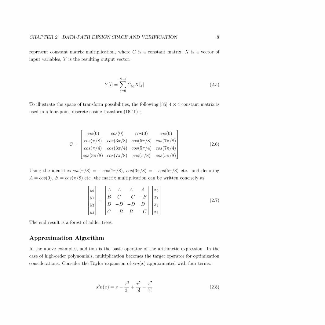
CHAPTER 2. DATA-PATH DESIGN SPACE AND VERIFICATION 8
represent constant matrix multiplication, where C is a constant matrix, X is a vector of
input variables, Y is the resulting output vector:
Y [i] =N−1∑j=0
Ci,jX[j] (2.5)
To illustrate the space of transform possibilities, the following [35] 4× 4 constant matrix is
used in a four-point discrete cosine transform(DCT) :
C =
cos(0) cos(0) cos(0) cos(0)
cos(π/8) cos(3π/8) cos(5π/8) cos(7π/8)
cos(π/4) cos(3π/4) cos(5π/4) cos(7π/4)
cos(3π/8) cos(7π/8) cos(π/8) cos(5π/8)
(2.6)
Using the identities cos(π/8) = −cos(7π/8), cos(3π/8) = −cos(5π/8) etc. and denoting
A = cos(0), B = cos(π/8) etc. the matrix multiplication can be written concisely as,y0
y1
y2
y3
=
A A A A
B C −C −BD −D −D D
C −B B −C
x0
x1
x2
x3
(2.7)
The end result is a forest of adder-trees.
Approximation Algorithm
In the above examples, addition is the basic operator of the arithmetic expression. In the
case of high-order polynomials, multiplication becomes the target operator for optimization
considerations. Consider the Taylor expansion of sin(x) approximated with four terms:
sin(x) = x− x3
3!+x5
5!− x7
7!(2.8)

CHAPTER 2. DATA-PATH DESIGN SPACE AND VERIFICATION 9
This polynomial of degree 7 approximates the sine function very well. Assuming the terms,
S3 = 1/3!, S5 = 1/5!, S7 = 1/7!
are pre-computed, the naive evaluation of the polynomial requires 3 additions/subtractions,
12 variable multiplications and 3 constant multiplications. However, it is possible to compute
this using the following sequence:
d1 = x · x (2.9)
d2 = S5 − S7 · d1 (2.10)
d3 = d2 · d1 − S3 (2.11)
d4 = d3 · d1 + 1 (2.12)
sin(x) = x · d4 (2.13)
Thus only 3 additions/subtractions, 4 variable multiplications and one constant multiplica-
tion are needed.
Another example where high-order polynomials are used for approximation is in (2.14 )
below. This is used in computing quadratic splines, which are used in computer graphics.
Such polynomials have degrees not more than 4, and are smooth in both the first and second
derivative and continuous in the third derivative.
P = zu4 + 4avu3 + 6bu2v2 + 4uv3w + qv4 (2.14)
The original formula (2.14) requires 23 multiplications and 4 additions. The following three
techniques transform the above polynomial into different implementations.
1. Two-term CSE (common sub-expression) algorithm:
d1 = u2 (2.15)
d2 = v2 (2.16)
d3 = uv (2.17)
P = d1z + 4ad1d3 + 6bd1d2 + 4wd2d3 + qd22 (2.18)
2. Using the Horner form:
P = zu4 + v · (4au3 + v · (6bu2 + v · (4uw + qv))) (2.19)

CHAPTER 2. DATA-PATH DESIGN SPACE AND VERIFICATION 10
3. Using algebraic factoring:
d1 = u2 (2.20)
d2 = 4v (2.21)
P = u3 · (uz + ad2) + d1 · (qd1 + u · (wd2 + 6bu)) (2.22)
Optimization Method Num Multiply Num AddTwo-term CSE 16 4
Horner 17 4Algebraic 13 4
Table 2.1: Result of three data-path transformations
Table 2.1 shows the number of variable multiplications and addition operations needed after
the design transformations. The actual implementation decision depends on the context,
design constraints and the surrounding logic in which these polynomials are to be imple-
mented.
Equivalence checking of individual multipliers is a well-known challenge already, but verifi-
cation of these transformed polynomials is even more difficult. This further motivates the
need to reason at a higher level rather than purely at the Boolean level.
2.3 About Adding a Set of Numbers
In the above data-path optimization procedures, addition is a basic operation. Multiplier
design is a good example of this. An n-bit binary number itself, A = an−1an−2 . . . a1a0, is
defined using a binary integer format by adding n numbers together:
A =n−1∑i=0
2i · ai (2.23)
B =n−1∑j=0
2j · bj (2.24)
Then, the multiplication two n-bit binary numbers, equation (2.25), can be seen as a sum
of n × n partial products of 2iai · 2jbj, which forms an n × n matrix in Figure 2.1. While

CHAPTER 2. DATA-PATH DESIGN SPACE AND VERIFICATION 11
implementing the multiplier, one has to decide the order in which these partial-products are
be added, .e.g. equation (2.25) adds the columns first, while (2.26) adds the rows first.
A×B =n−1∑i=0
n−1∑j=0
2i+j · ai · bj (2.25)
B × A =n−1∑j=0
n−1∑i=0
2i+j · ai · bj (2.26)
0 i n− 1
n−1
j
a0b020 a1b021 a2b022 · · · aib02i · · ·
a0b121 a1b121+1 a2b122+1 · · · aib12i+1 · · ·
......
......
a0bj2j a1bj2
1+j a2bj22+j · · · aibj2
i+j · · ·
......
......
Figure 2.1: A×B = Sum of n2 partial products
Multiplication is commutative: A × B ≡ B × A. However, these two multiplier implemen-
tations results in a Boolean satisfiability problem from A×B ≡ B ×A that is very difficult
to solve at the bit level. This is because the two multiplier logics are completely different
internally, and applying knowledge of the commutative law at the Boolean level is all but
impossible.
2.4 Empirical Study: Eight-Operand Adder-Tree
Equivalence Checking
From the above survey, addition is seen to be the basic operator for adder-trees and multiplier
implementations. In this section, we evaluate the capacity and performance of the SAT-
sweeping procedure in proving pure adder-trees equivalence. As SAT-solving is classified as
an NP-complete algorithm, we wonder in what situations it gets easier and in what situations

CHAPTER 2. DATA-PATH DESIGN SPACE AND VERIFICATION 12
it gets more difficult. We use the following case-study to help understand the strengths and
weaknesses of Boolean methods. The objective is to show that a Boolean solving method has
inherent limitations which cannot be resolved within itself; in order to solve these data-path
equivalence checking problems, higher level information needs be captured to help reduce
the problem complexity. This leads to our belief that we have to enable a tool to reason
beyond Boolean logic.
module LinearAdderTree
#(
parameter WIDTH = 16)
(
input [WIDTH-1:0] a[7:0],
output [WIDTH+4-1:0] y) ;
reg [WIDTH+4-1:0] ret;
always_comb begin
ret = 0 ;
for (int i=0;i<7;i++)
ret = ret + a[i];
end
assign y = ret;
endmodule
Figure 2.2: Linear Adder Tree described in Verilog
The Verilog code in Figure 2.2 implements an eight-operand addition in integer arithmetic:
the use of the WIDTH parameter definition guarantees there are no overflow situations.
There are many ways to implement such an adder tree logic. Figure 2.3 shows four examples
using linear tree or binary tree topologies, and with different orders of adding terms. Table 2.2
compares the internal similarities between the four structures. Columns 1 and 2 are the two
structures being compared. Column 3 gives a ranking of the amount of internal structural
similarity between the compared adder-trees. Column 4 shows terms where similarities
exist. The first two pairs share the top similarity ranking as they are symmetric and have
the same amount of internal similarities. The third pair has slightly more similarities than
the remaining three pairs because the two adder tree structures are symmetric and both are
full binary trees. The remaining three pairs are dissimilar in roughly the same degree. The

CHAPTER 2. DATA-PATH DESIGN SPACE AND VERIFICATION 13
Linear Adder Tree Reversed Linear Adder Tree Binary Adder Tree Justaposed Binary Adder Tree
a0 a1
+ a2
+ a3
+ a4
+ a5
+ a6
+ a7
+
+
a6 a7
+
a5
+
a4
a3
+ a2
+ a1
+ a0
+
+
a0 a1
+
a2 a3
+
a4 a5
+
a6 a7
+ +
+
+
a0 a7
+
a1 a6
+
a2 a5
+
a3 a4
+ +
+
Figure 2.3: adder tree structure.
significance of the similarities are illustrated in the following experiments, which conducted
equivalence checking between the varous pairs.
Adder0 Adder1 Similarity Rank SimilaritiesLinear Binary 1st a0 + a1 , ((a0 + a1) + (a2 + a3))
Reversed Linear Binary 1st a6 + a7 , ((a4 + a5) + (a6 + a7))Binary Juxtaposed Binary 3rd a0 + a1 , a6 + a7 vs. a0 + a7 , a1 + a6
Linear Reversed Linear 4th NoneLinear Juxtaposed Binary 4th None
Reversed Linear Juxtaposed Binary 4th None
Table 2.2: Internal similarities between Adder Trees in Figure 2.3
We conducted equivalence-checking between these four adder-tree structures using ABC[2]’s
dcec command, which is a state-of-art combinational equivalence checking procedure using
SAT-sweeping at the bit-level. Such a procedure uses SAT solvers as the main solving engine
to establish equivalence by identifying and utilizing internal match-points, i.e. signals in the
design that are functionally equivalent to each other. Figure 2.4 shows the run-time results
on pair-wise equivalence checking with operand WIDTH from 1 to 35.
Comparing with Table 2.2, the run-times inversely follow the rankings in similarity. The first
two pairs of comparison scale well with WIDTH while the others do not scale. As illustrated
in Figure 2.5, the complexity of solving equivalence checking problem ranges from constant
time to apparently exponential time; the actual difficulty depends on the amount of internal

CHAPTER 2. DATA-PATH DESIGN SPACE AND VERIFICATION 14
Figure 2.4: ABC’s dcec results
similarities. On the left side is the extreme case that both logic structures are exactly the
same, then equivalence can be determined through structural hashing; the output functions
are hashed into the same node value. On the right side is the other extreme; logic equivalence
has to be established through exhaustively searching the entire Boolean function space: i.e.
solving an NP-complete problem.
more
StructuralSimilarity less
Structural hashingO(1)
Boolean SatisfiabilityNP-Complete
Figure 2.5: Complexity scale of SAT-Sweeping
The total number of different n operand adder trees is P nn ×
∏2i=nC
2i . From the complex-
ity growth of the 8-operand adder tree example, it seems that pure Boolean methods are
unable to solve problems where design transformations render them structurally dissimilar.
Knowledge of high-level design functionality is seemingly required.

CHAPTER 2. DATA-PATH DESIGN SPACE AND VERIFICATION 15
2.5 Survey: Data-Path Formal Verification
Techniques
Boolean logic is defined over Boolean space B, B = {0, 1}. A Boolean function f of m
variables is a mapping of Bm → B. Boolean logic functions can be represented as a directed
acyclic graph, with each node annotated as a Boolean function, such as an and-invertor
graph (AIG). A bit-vector is a set of Boolean variables; a bit-vector function is a collection
of Boolean functions.
For convenience, we will refer to a single Boolean variable as a bit, a bit-vector as a word,
a function over words as a word-level function or word-level operators. A network which
contains word-level operators is called a word-level network.
As illustrated in Figure 2.6, the bit-blasting procedure transforms a word-level operator into
a set of bit-level functions; the inverse of this, the procedure to group bit-level functions
into word-level operators is sometimes called reverse-engineering, a significantly difficult
operation.
networkbit-level word-level
networkreverse engineering
bit-blasting
Figure 2.6: Bit-level to word-level transformation
The data-path logic discussed in this thesis refers to any set of arbitrary bit and word-level
operators. The focus of the techniques to be developed in this thesis to analyze data-path
logic, is to use reasoning on the word-level operators to help in checking bit-level equivalence.
Conceptually, data-path logic specification provides the following :
1. a directed graph, with nodes annotated as word level operators with specified input
and output widths.
2. the word-level operators are from a known library of arithmetic functions.
The remaining sections in this chapter gives an overview of the various techniques available,
from Boolean solving to pure theorem proving of first order logic.

CHAPTER 2. DATA-PATH DESIGN SPACE AND VERIFICATION 16
Boolean Solvers
Boolean solving techniques are fundamental and generic in that all data-path logic can be
converted into Boolean functions. There are essentially four basic categories for establishing
that two Boolean networks are equivalent:
1. Structurally the same
2. Equivalence through exhaustive simulation
3. Equivalence established by SAT solving
4. Equivalence established by BDDs
One direction in optimizing Boolean solvers is to improve the performance of the SAT solver
and BDD packages. The other direction is to simplify the Boolean logic structure through
transformations. The technique of the SAT-sweeping procedures in [12] uses all four cate-
gories, structural hashing, simulation, SAT, and BDDs to identify and merge internal equiv-
alent points, thus reducing overall complexity. In [70], the authors further attempted to
find more internal points to merge by extending the definition of equivalent nodes under the
condition of observability don’t cares. [11] tries to minimize intermediate BDD size through
converting a BDD relation into a corresponding parametric representation with a smaller
set of BDD variables. State-of-art equivalence checking procedures [52] provides a highly
integrated and optimized implementation of AIG [43] rewriting, simulation, SAT-sweeping
and logic synthesis techniques. This has led to dramatic improvements over earlier imple-
mentations.
The advantage of these Boolean solvers is that they are generic and fully automated. They
are very good at finding discrepancies and providing error traces if the designs are not
equivalent. However, on proving equivalence, their strengths becomes their own weakness,
as the complexity is NP-complete. If two designs are structurally dissimilar, then obtaining
an equivalence proof can be very difficult. On the other hand, there can exist a trivial proof
even when structural dissimilarity exists, e.g. for summing eight integers, equivalence can
be established through commutative, associative and distributive laws of the ’+’ operator.
Clearly an advantage can be obtained if knowledge of the ’+’ operator can be integrated into
the Boolean solving methods.

CHAPTER 2. DATA-PATH DESIGN SPACE AND VERIFICATION 17
The Use of Un-Interpreted Functions (UIFs)
The use of un-interpreted functions (UIFs) tries to simplify the equivalence checking program
by introducing constraints from the functional level. The principle of UIF derives from the
general definition of what is a function: a function is a mapping from its input domain to
its output domain which requires that for the same inputs, the output is always the same:
if f ≡ g then
∀X∀Y, s.t. X = Y ⇒ f(X) = g(Y )
We use the miter logic formulation in Figure 2.7 to illustrate the utilization of the knowledge
of a function. In Figure 2.7, the left side has two multiplier instances while the right side has
only one; this might have been the result of minimizing the number of computation units
during an optimization phase. If the multipliers are wide, it is a difficult problem to prove
equivalence using purely Boolean techniques.
* *
a b c dsel
F = sel ? (a*b) : c*d)
*
G = (sel ? a:c) *(sel? b:d)
g h
j k
i m
=?
miter
mux
mux mux
Figure 2.7: Use of UIF
For this particular design, the detailed functionality of the multiplier is not needed proving
the logic equivalence. In this case, the multiplier function can be replaced with any function,
and the equivalence would still hold provided the two functions being paired are the same
function. The UIF technique utilizes such an observation and performs the following two
steps:

CHAPTER 2. DATA-PATH DESIGN SPACE AND VERIFICATION 18
• Remove the internal logic of each multiplier and create new free-input variables for
each multiplier output.
• Add the following constraints/lemmas to the miter logic
(a = j) & (b = k) ⇒ m = g (2.27)
(c = j) & (d = k) ⇒ m = h (2.28)
and similarly when j and k are interchanged. Each of these implications is known as a UF
constraint. In this case, a UF constraint is put between every multiplier on the left and every
one on the right. By taking advantage of the knowledge that functions m, g and h are the
same functions, the transformed Boolean satisfiability problem is then easily proven using
SAT solvers, thereby proving the original problem. Note that even if the internal logic of
the multipliers is not removed, the UF constraints still can be asserted and may be effective
because they establish a relation between the two halves of the miter to be proved equivalent.
Note also that although the UF constraints are implied by the Boolean logic of the miter,
it would be essentially impossible to establish this from reasoning at the bit-level. This
information comes from a higher level knowledge that m, g and h are the same functions.
Satisfiability Modulo Theory(SMT) Solvers
The UIF approach is the simplest framework to utilize the knowledge that part of the design
is implementing a high-level function, while the details of the function’s definition are not
needed. To extend the use of high-level functions, the next level is to be able to reason
about a function’s input/output definition. In the data-path equivalence checking domain,
it requires the prover to represent and reason about quantifier-free first order logic.
Formally, an SMT instance [59] is a formula in quantifier-free first-order logic, and SMT
is the problem of determining whether such a formula is satisfiable. Imagine a Boolean
SAT instance in which some of the binary variables are replaced by ”predicates” over a
suitable set of non-binary variables. A predicate is basically a binary-valued function of non-
binary variables. Example predicates include (integer) linear inequalities (e.g., 3x+ 2y > 6,
z >= 4) or equalities involving so-called uninterpreted terms and function symbols (e.g.,
f(f(u, v), v) = f(u, v) where f is some unspecified function of two unspecified arguments.)
We are still dealing with a satisfiability problem, except that its solution now depends on
our ability to determine the satisfiability of the underlying predicates.

CHAPTER 2. DATA-PATH DESIGN SPACE AND VERIFICATION 19
In summary, an SMT instance is a generalization of a Boolean SAT instance in which various
sets of variables are replaced by predicates from a variety of underlying theories. Practically,
SMT formulas provide a much richer modeling language than what is possible with Boolean
SAT formulas. In particular, for data-path equivalence checking, the QF BV SMT [59]
constructs allows us to model the data-path operations at the word rather than the bit level,
which is equivalent in expressiveness to Verilog operators.
Early attempts at solving SMT instances involved translating them to Boolean SAT instances
(i.e. bit-blasting the word-level operators into bits) and passing this (much larger) formula
to a Boolean SAT solver. This approach has its merits: by pre-processing the SMT formula
into an equivalent Boolean SAT formula we can use existing Boolean SAT solvers ”as-is” and
leverage their performance and capacity improvements over time. On the other hand, the
loss of the high-level semantics of the underlying theories means that the Boolean SAT solver
has to work a lot harder than necessary to discover ”obvious” facts (such as x · y = y · x for
integer multiplication.) This observation was the impetus behind the development, over the
last several years, of a number of SMT solvers that tightly integrate the Boolean reasoning
of a DPLL-style search with theory-specific solvers that handle conjunctions (ANDs) of
predicates from a given theory.
Dubbed DPLL(T) [63], or Generalized DPLL [50], this architecture gives the responsibility
of Boolean reasoning to the DPLL-based SAT solver which, in turn, interacts with a solver
for theory T through a well-defined interface. The theory solver need only worry about
checking the feasibility of conjunctions of theory predicates passed on to it from the SAT
solver as it explores the Boolean search space of the formula. For this integration to work
well, however, the theory solver must be able to participate in both propagation and conflict
analysis, i.e., it must be able to infer new facts from already established facts, as well as
to supply succinct explanations of infeasibility when theory conflicts arise. In other words,
the theory solver must be incremental and back-trackable while the theory’s implementation
varies and is domain-specific.
Relevant to the data-path equivalence checking problems is the SMT QF BV(Quantifier Free
Bit Vector Arithmetic) solvers. One of its contributions is the introduction of word-level
operators that allows word-level structures to be represented in the problem formulation.
In some of the leading SMT solvers [13][23][34], word-level techniques such as rewriting,
abstraction refinement and reduction etc. are applied. Depending on the underlying theory

CHAPTER 2. DATA-PATH DESIGN SPACE AND VERIFICATION 20
used or extracted from the QF BV formulation, the generalized DPLL framework is used
to integrate the Boolean SAT solvers. Furthermore, when the problem remains unsolved,
bit-blasting the QF BF formulation into a CNF formula is the last resort for most of the
leading SMT bit-vector solvers, Boolector [13], z3 [23], Beaver [34]. If this bit-blasting does
not solve the problem, the programs terminate without an answer.
The advantages of SMT solving using the Generalized DPLL framework are that it is a
generic, automated method and empirically often effective in finding counterexamples if the
designs are not equivalent. However, this strength leads to a weakness that the SMT solvers
still treats the underlying problems as a Boolean satisfiability problem which is inherently
NP-complete – potentially very difficult or impossible to solve.
Theorem Proving
While Boolean SAT solvers inherently are solving an NP-Complete problem, theorem prover
attempts to provide an alternative. By reasoning in first order logic, a theorem prover
integrates Boolean logic and high-level functions natively. In comparing to a pure theorem
proving approach, SMT solving is a hybrid approach as it has the ability to represent first
order logic for a specialized theory and integrates Boolean solvers at the same time. For
theorem proving in the data-path equivalence checking domain, the subject of interest is
quantifier-free first order logic. We use an example, from [36], to illustrate the thought
process of theorem proving. We show that theorem proving is not only a method but also a
necessity in its problem formulation. Theorem proving differs fundamentally from Boolean
solvers because a proof is based on symbolic rewriting and mathematical induction rather
than Boolean SAT solving – hence theorem proving does not try to solve the data-path
equivalence checking problem as an NP-complete problem.
The Verilog module in Figure 2.8a implements a 32-bit ripple-adder and we create an equiv-
alence checking problem by comparing it with adder32 in Figure 2.8b:
ripple adder32 ≡ adder32 (2.29)
The proof objective is the following:
Does above (2.29) check that Verilog module ripple adder32 implement the ad-
dition of two binary integer numbers correctly.

CHAPTER 2. DATA-PATH DESIGN SPACE AND VERIFICATION 21
module ripple_adder32(
input cin,
input [31:0] a0,
input [31:0] a1,
output reg [31:0] o,
output reg cout ) ;
always_comb begin
cout = cin;
for (i=0;i<32;i++) begin
o[i] = a0[i] ^ a1[i] ^ cout;
cout = (a0[i] & a1[1])
| (a0[i]& cout)
| (a1[i] & cout);
end
end
) ;
endmodule
(a) Verilog Ripple Adder
module adder32(
input cin,
input [31:0] a0,
input [31:0] a1,
output [31:0] o,
output cout ) ;
assign cout,o = a0 + a1 + cin;
endmodule
(b) Verilog Adder
The answer seems to be a either “YES” or “NO”, but the truth is: the equivalence checking
of (2.29) cannot answer the question. The reason is a problem formulation mismatch : the
proof objective is about natural numbers adding together, whereas the Verilog module is in
the Boolean domain which does not have the concept of what a natural number is. The
above proof objective about integer addition can not be answered in the Boolean domain
solely (i.e. using the formula 2.29), because in Boolean logic, one cannot reason about ’+’
in integer domain. To prove ripple adder32 correctly adds two natural numbers together,
first order logic is needed to express what is a natural number, as well as to formulate the
definition of ’+’ as a function connecting it to Boolean logic.
Thus the objective of the verification is no longer a data-path equivalence checking problem at
the RTL level, but a mathematical one using first-order logic. We use ACL2 to illustrate such
a process by constructing a ripple adder in ACL2 and illustrate the correctness formulation
along with the proof procedure.

CHAPTER 2. DATA-PATH DESIGN SPACE AND VERIFICATION 22
Name Axiom, Definition, or TheoremThm 1 t 6= nilAX 2 x = nil −→ ( if x y z ) = zAX 3 x 6= nil −→ ( if x y z ) = y
Def not (not p) = ( if p nil t)Ax 4 (car (cons x y)) = xAx 5 (cdr (cons x y)) = yAx 6 (consp (cons x y)) = t
Thm 7 (endp x) = (not (consp x))
Table 2.3: ACL2 Axioms
ACL2 Introduction
ACL2 functions and theorems are established using a small set of basic axioms and theorems.
Everything else is constructed from these basic logic elements. Table 2.3 shows the list of
Axioms and Theorems that are used by the ACL2 theorem prover [37]. The first four define
two basic values t and nil, along with the definition of the if and not functions. Note,
they are just symbols, although t and nil can be thought of as true and false in Boolean
logic. Computation in ACL2 logic is symbolic, using the rules of substitution, inference, and
mathematical induction. In ACL2, a list is also a first order object. cons is the function that
takes an element and a list as inputs, and prepends the element to the head of the list. The
Operator car gets the first element of the list, while cdr gets the rest of the list by removing
the head of the list.
To illustrate the semantics, we use Python to model the car and cdr functions as follows:
def car(lx) :
if lx == nil :
return nil
assert len(lx) > 0
return lx[0]
def cdr(lx):
if lx == nil or len(lx) == 1:
return nil
else :

CHAPTER 2. DATA-PATH DESIGN SPACE AND VERIFICATION 23
return lx[:-1]
pass
By ACL2 definition, it is illegal to call car over an empty-list value, but car over nil returns
nil, so does cdr (nil is not equivalent to the empty-list value). In Ax 6, the predicate ’consp’
returns t if its operand can be represented as (cons x y). endp is the opposite of consp. So
we have the following results:
( car nil ) = nil
( cdr nil ) = nil
( car (cons t nil) ) = t
( cdr (cons t nil) ) = nil
(endp (const t nil)) = nil
(consp (const t nil)) = t
ACL2 Boolean Logic Definition
Using ACL2 functions, the following defines Boolean-valued functions : and , or, xor and
the majority function(bmaj).
(defun band (p q ) ( if p ( if q t nil ) nil ) )
(defun bor (p q ) ( if p t ( if q t nil ) ) )
(defun bxor (p q ) ( if p (if q nil t ) (if q t nil) ) )
(defun bmaj (p q c )
(bor ( band p q)
( band p c )
( band q c ) ) )
A full adder function has three inputs (bits) and returns a multi-value (mv is the keyword
for multi-value) : a sum and a carry, which is defined as follows:
(defun full-adder ( p q c )
( mv (bxor p ( bxor q c ) )

CHAPTER 2. DATA-PATH DESIGN SPACE AND VERIFICATION 24
( bmaj p q c)
) )
A serial-adder is defined as :
(defun serial-adder (x y c)
( if ( and (endp x) (endp y))
(list c)
(mv-let (sum cout)
(full-adder (car x) (car y) c)
(cons sum (serial-adder cdr x) (cdr y) cout )))))
This is a recursive definition of a ripple-adder tree. The bit-vectors x and y are ordered
lists of binary values, i.e. nil and t. The least significant bit of the bit-vector (LSB) is the
first element and most significant bit (MSB) is the last element in the lists x and y. The
operation (car x) returns the LSB of x and (cdr x) returns the rest of the bits. In ACL2,
value nil and a list of nil values are practically the same, as car and cdr on both values
return nil. Because of this, the above formulation doesn’t require x and y to have the same
length. One can think of the shorter operand as having been appended with nil, just as the
high order bits of a binary number is prepended with 0.
ACL2 Integer and Integer Addition Definition
The following function ’n’ is defined that maps a binary integer number from the list of t
and nil values:
(defun n (v)
(cond ((endp v) 0)
((car v) (+ 1 ( * 2 (n (cdr v)))))
(t (* 2 (n(cdr v))))))
To illustrate the above semantics in Python, the function n would be defined as follows:
def n(v):
if len(v) == 0:

CHAPTER 2. DATA-PATH DESIGN SPACE AND VERIFICATION 25
return 0
elif v[0] == True:
return 1 + 2*n(v[1:])
else :
return 2 * n(v[1:])
ACL2 Proof of Serial Adder Implementation
Both + and ∗ operators are first class objects and are just symbols, which carries no com-
putational semantics. The proof obligation of correctness of the serial-adder is formulated
as the following theorem:
(defthm serial-adder-correct
(equal (n (serial-adder x y c)
(+ (n x) (n y) (if c 1 0)))))
The above is essentially proving that adding x, y, c together using + is the same as the
natural number obtained after they are added together using the serial-adder function.
n(serial-adder(x, y, c)) ≡ n(x) + n(y) + n(c) (2.30)
The proof is obtained by mathematical induction. The reader can check the basic step of
the induction. For the inductive step, ACL2 effectively checks the following implication:
(implies (= (n (serial-adder x y c))
(+ (n x) (n y) (n c)))
(= (n (serial-adder (cons x0 x) (const y0 y) c))
(+ (n (cons x0 x)) (n (cons y0 y)) (if c 1 0)))
)
In English, the above is proving that if serial-adder is correct for list x and list y then
serial-adder would be correct for list (x0 x) and list (y0 y), i.e. the lists with one more
element prepended to the front. ACL2 has rigorous theories and procedures for reasoning
using induction, and for the scope of this thesis, ACL2 obtains the proof by proving the
following two lemmas first:

CHAPTER 2. DATA-PATH DESIGN SPACE AND VERIFICATION 26
(defthm serial-adder-correct-nil-nil
(equal (n (serial-adder x nil nil))
(n x)
))
(defthm serial-adder-correct-nil-t
(equal (n (serial-adder x nil t))
(+ 1 (n x ))
))
Not so surprisingly, the above two lemmas are proving that the serial-adder is adding ’0’ and
’1’ correctly. Different from Boolean equivalence checking, the proof of correctness is generic
over any length of input list x and list y.
The above proof formulation and proof is not a data-path equivalence checking problem
where two Boolean logics are compared. However, the theorem prover approach can be
applied to data-path equivalence checking as a bridge: the proof is obtained by proving
both designs implement the same high-level function. In our example, the equivalence of the
adder trees in Section 2.4 can be established if we can prove they all implement the same
binary-number-adding function, e.g.
(defthm adder-tree-correct
(equal (n (any-adder-tree x y c)
(+ (n x) (n y) (if c 1 0 )))))
Theorem Proving Summary
In the ACL2 methodology for data-path equivalence checking, SAT-sweeping in the Boolean
domain is not used; instead, it uses a proxy function in first order logic to establish the
equivalence. Theorem proving is a complementary approach to Boolean solvers as it does
not explore the Boolean space, therefore it does not need to solve an NP-Complete problem.
First order logic is expressive enough to formulate any arithmetic or algebraic function. In
theory, for equivalent data-path designs, a proof can always be constructed using a theorem

CHAPTER 2. DATA-PATH DESIGN SPACE AND VERIFICATION 27
prover. Although this seems to be a promising technique by not casting into an NP-complete
problem, in practice, theorem proving has very limited applications for three reasons:
1. It is a usability issue. Designs are mostly expressed in hardware or software program-
ming languages. To reason in first order logic, designs must be translated into first
order logic which imposes extra overhead required for debugging and validation. Also,
first order logic is an abstract and difficult-to-use language for most people, and only
for very specific application domains is the theorem proving method used.
2. The main strength of theorem proving is mathematical induction, which is also a
weakness. For it to work, the target function needs to have a regular pattern such that
it can be defined recursively. A recursive definition framework may fit for arithmetic
functions such as integer addition, multiplications, divisions etc, but it is unsuited for
arbitrary Boolean control logic. For this particular reason, theorem provers are limited
practically to proofs in the purely arithmetic domain. There are two natural directions
to improve the application of theorem proving. One is to build extensive libraries such
that it can be applied to more complex functions. In ACL2, these are called ACL2
books. The other direction is to incorporate Boolean engines into the theorem prover
by integrating the definitions of AIGs and SAT solvers in order to handle arbitrary
Boolean logic. To preserve the rigor of theorem proving, AIG and SAT solvers need
to be defined from the ground up. Once this is done, the usability of theorem proving
can be extended to more complex design spaces.
3. Successful application of theorem proving techniques requires a deep understanding of
the design implementation because the proof is obtained through breaking down inter-
nal structures. From the ripple-adder example, the proof is built upon the recursive
structure of the ripple-adder implementation. The implication of such a proof is that
the verification effort may not be reusable: a change in the design internals may poten-
tially require a completely different proof. Also, it takes effort and is a productivity cost
to gain such deep knowledge of a design’s internal details. On the other hand, using
simulation or Boolean solving methods, verification engineers only need to model the
design functionality at the interface level and the validation model is reusable as long
as the design functionality remains the same – the internal implementation decisions
and changes do not impact the validation model.

CHAPTER 2. DATA-PATH DESIGN SPACE AND VERIFICATION 28
In the next Chapter, we present our LEC data-path equivalence checking system which has
the following characteristics:
• LEC’s ultimate goal is to find a way to solve all data-path equivalence checking prob-
lems.
• For ease of use, LEC uses Verilog/VHDL as the input language and retains the original
design structure throughout the proof finding process.
• Similar to ACL2 books, the LEC system achieves reuse by integrating new techniques
into an existing system, and thus LEC becomes more powerful when it is applied to a
new problem domain.
• As design knowledge is needed inevitably to obtain a proof, LEC is a learning aid to
extract and understand logic that presents a bottleneck in the proof process.
LEC is extensible. Building and using LEC are both learning processes, while the learning
is expedited by LEC.

29
Chapter 3
LEC: Learning-Driven Equivalence
Checking
We build a system to learn,
expand and grow with the
unknown.
The problem formulation in this chapter is to compare two logic functions, F and G , for
equivalence :
∀x F (x) = G(x) (3.1)
Both F and G are combinational logic circuits described in Verilog/VHDL. For equivalence
checking, a miter logic, shown in Figure 3.1, is formed to compare the two. The formulation
is also a Boolean satisfiability model of trying to satisfy F 6= G. The proof result is either
UNSAT if F ≡ G , SAT if F 6= G or UNRESOLVED if F ≡ G can not be determined.
3.1 Overview: A Learning Process - Philosophy
One of the key aspects of this work is to view the equivalence checking problem as a learning
process and to implement a Learning-Driven Equivalence Checking (LEC) tool flow to enable
and expedite the process. Our learning process and our implementation of LEC recognizes
that:

CHAPTER 3. LEC: LEARNING-DRIVEN EQUIVALENCE CHECKING 30
y = F (x) y = G(x)
=?
inputs: x
miter
Figure 3.1: Miter logic
1. There will always be a new problem that can not be resolved,
2. But a LEC-type tool can be extended to solve many un-solved problems.
This is a limited claim because the data-path optimization techniques in the previous chapter
would seem to be able to introduce a new miter problem that is beyond LEC’s current proof
capabilities. On the other hand, LEC is implemented to enable learning about un-solved
problems encountered, identifying bottleneck components and discovering and enabling new
techniques to solve them. Hence, we expect that our LEC system (henceforth just called
LEC) should evolve over time. We believe that
1. every unsolved miter logic is an opportunity for LEC to grow, improve and become
more powerful,
2. by using LEC, we can gain knowledge of the underlying Boolean logic, identify bottle-
neck components, reverse engineer and abstract it into high-level arithmetic or algebraic
formulae, and that
3. learning itself expedites future learning.
LEC is architected to facilitate the integration of different approaches, automate reuse of
implemented methods, and enable the development of new techniques in future applications.

CHAPTER 3. LEC: LEARNING-DRIVEN EQUIVALENCE CHECKING 31
In some sense, every tool development is a learning process. However, we embrace this as a
strategic view and try to build LEC to enable and expedite learning for both user and tool
developer. The LEC system is designed with an open architecture so that it can be used
also as a manual aid to unravel a miter logic. The process to get to a proof should be one
that gradually learns about the design and develops/integrates new techniques which help
to transform an unknown into an identified unknown, and eventually to a known.
3.2 Tool Flow and Organization
LEC takes Verilog/VHDL designs as inputs and is divided into a front-end and a back-
end, with a WNK (word-level-network) as an intermediate representation. A WNK is a
data-structure that explicitly represents the bit-vector arithmetic operators expressed in
Verilog language or SMT QF BF specification[59]. Shown in Figure 3.2, the LEC front-end
uses a Verific RTL parser [64] to compile the input RTL into the Verific Netlist Database
and then translates this into a WNK. The Verific Netlist Database is a graph structure
that captures the design hierarchy and connectivity information. Our VeriABC[48] system
processes a Verific Netlist, flattens the hierarchy and obtains a WNK representation, which
captures the circuit function topologically. Except for the hierarchical information, WNK
is a close-to-verbatim representation of the original RTL description. Most importantly, it
keeps all high-level information of the original RTL. A WNK is the central core of the LEC
infrastructure.
The LEC back-end consists of a set of widgets which perform various transformations, solving
tasks, or learning tasks on WNK data structures. The use-model of LEC is a sequence of
recursive applications of the LEC widgets.
Word-Level Network(WNK)
A LEC word-level network(WNK) is a directed acyclic graph representing the logic function.
Each node in the graph contains three attributes: operator type, width, and an array of
fanin nodes. In Figure 3.3 it is defined in the C + + class definition.
(rkb you have two captions here???)
The type of operator indicates the logic function at the node. Table 3.1 lists the unsigned

CHAPTER 3. LEC: LEARNING-DRIVEN EQUIVALENCE CHECKING 32
Originalmiter
Verific Parser Frontend
WNK
SimulationWidget
ABCsolvers
VeriABC
TransformationWidgets
Bit−blastWidget
TransformedRTL
newmiter target
UNSATSAT
Figure 3.2: Overall tool flow
class wnode_s {
const operator_type_t _operator;
const int _width;
const int _num_fanins;
wnode_s * _faninx[] ;
} ;
Figure 3.3: Illustration WNK node in C++ class
operators in WNK which correspond to the operators in the Verilog language definition. The
operators also have their equivalents in the SMT QF BV[59] specification. Along with the
operator attributes, the node is associated with an integer width to indicate the length of
the bit-vector it represents. The incoming edges at a node are represented by the faninx
array.
Verilog operator types SMT QF BV operator types
Boolean &&, ‖, !,⊕,mux and, or, not, xor, ite
bit-wise &, |,∼,⊕,mux bvand, bvor, bvnot, bvxor, bvite
arithmetic +,−, ∗, /,% bvadd, bvsub, bvmul, bvdiv, bvmod
extract [] extract
concat {} concat
comparator <,>,≤,≥ bvugt, bvult, bvuge, bvule
shifter �,� bvshl, bvshr
Table 3.1: Supported operators (unsigned)

CHAPTER 3. LEC: LEARNING-DRIVEN EQUIVALENCE CHECKING 33
Any synthesizable Verilog module can be translated to such a WNK, which has the same
expressiveness as SMT Bit-Vector Arithmetic. Book-keeping information is kept during the
translation so that the signal names in the Verilog source code are mapped onto the WNK
nodes. A topological traversal of the network from inputs to outputs evaluates the output
logic function depending on the input values. For LEC, the WNK structure is self-contained
as it captures both the structural and functional information of the miter logic. Learning,
reasoning and transformations are executed on this structure.
3.3 The LEC Widgets
The LEC back-end is organized as a collection of widgets. LEC proofs are obtained through
iterative applications of these widgets. LEC has three categories of widgets based on their
functionality:
1. Solver widget,
2. Transformation widget,
3. Learning widget.
The LEC proof process is illustrated in Figure 3.4. Solver widgets are used to solve the
problem directly, which can return SAT, UNSAT or UNRESOLVED as the proof result. If
it returns UNRESOLVED, then learning and transformation widgets are applied to try to
transform the unresolved problem into a set of sub-models. These can be seen as lemmas
derived/decomposed from the original model. Each such lemma sub-model is a possible
proof target in the next LEC iteration. A LEC iteration basically calls LEC again so that
all the widgets can be used to break down the unresolved parts further. The final LEC proof
consists of an iterative application of these widgets.
Solver Widgets
The goal of a solver widget is to produce a definitive answer: SAT or UNSAT. The following
lists the set of basic solver widgets currently implemented in LEC:
1. Random simulation using Verilator[60]

CHAPTER 3. LEC: LEARNING-DRIVEN EQUIVALENCE CHECKING 34
��
��Start
?
�����
@@@@@
��
���
@@
@@@
SolverWidgets
SAT/UNSAT
UNRESOLVED
?LearningWidgets
?Transformation
Widgets
6
Lemmas
- -��
��Done
Figure 3.4: Proof process
2. Word-level network simulation using a WNK
3. Parallel bit-level simulation on an AIG model
4. SAT-sweeping using ABC’s dcec and iprove [52] commands
5. LEC’s internal SAT solving over the AIG based on ABC’s minisat[25] implementation.
The first three use simulations as the underlying algorithm and the other two use SAT
sweeping algorithms. The set of solver widgets can be extended by integrating a set of
widgets together into a single composite widget (solver widget script), as long as the result
is able to return SAT, UNSAT given the proof target.
Transformation Widgets and Sub-model Trees
LEC proofs are built on the use of the transformation widgets. Each transformation widget
performs a deterministic function following a set of input instructions to convert the root
miter model into a set of sub-models. There is an implicit logical relationship between the
root model the generated sub-models, where logical inference rules are applied to derive the
sub-models from the root model. We would like to capture these inference rules explicitly to
record the proof process.
For logical inference, the most generic rule is modus ponens:

CHAPTER 3. LEC: LEARNING-DRIVEN EQUIVALENCE CHECKING 35
”if p then q” is accepted, and the antecedent (p) holds, then the consequent (q)
may be inferred.
In LEC, this is cast as an assume-guarantee (A/G) framework:
if the assumptions hold (i.e. are proven) then the satisfiability of original miter
model can be derived from the set of generated sub-model lemmas.
Lemma Types Inference Rule Example use scenariopre-lemmai preconditions: must all be proven UNSAT assume/guarantee reasoning
s-lemmaUNSAT (s-lemma)⇒ UNSAT (MM)SAT (s-lemma)⇒ SAT (MM)
structural hashing
e-lemmai∃i SAT (e-lemmai)⇒ SAT (MM)∧
i UNSAT (e-lemmai)⇒ UNSAT (MM)case-split enumeration
a-lemma UNSAT (a-lemma)⇒ UNSAT (MM) over-approximationu-lemma SAT (u-lemma)⇒ SAT (MM) under-approximation
Table 3.2: Lemma Types(MM is the current model)
Given the above insight, we explicitly captures the inference rules used in all LEC proofs
through the five lemma-types in Table 3.2. The satisfiability of the original miter model
MM is inferred from the satisfiability of its sub-model lemmas. The presence of pre-lemmai
captures the assumption components in the A/G reasoning, all of which need to be proven
UNSAT in order for this transformation to be valid. The rest of the lemma types are for
the ”guarantees” which are used to infer MM ’s proof results from its sub-model lemmas. An
s-lemma indicates equisatisfiability: its (un)satisfiability is equivalent to the (un)satisfiability
of original miter model MM . The {e-lemmai} set is the result of case-split enumerations
where their conjunction is equivalent to MM . An a-lemma is an over-approximation(e.g.
resulting from abstraction techniques), while the u-lemma is an under-approximation of the
original MM .
The method of lemma generation from the transformation widgets allows transformations
to be carried out arbitrarily, allowing both valid and invalid transformations during LEC
proof process. The correctness of the final LEC proof is guaranteed through the existence
of pre-lemmai: transformations with falsified or unresolved pre-lemmai are omitted from the

CHAPTER 3. LEC: LEARNING-DRIVEN EQUIVALENCE CHECKING 36
final proof construction. These invalid transformation intuitively corresponds to failed trial
efforts.
In summary the transformation widgets and the generated lemma sub-models achieve the
following:
1. The task of a LEC transformation widget is to perform an atomic operation which
transforms the current model into a set of lemma sub-models using a specific set of
inference rules. The widget is a deterministic function given a set of input instructions
on how the transformation is to be carried out – no complex procedures such as Boolean
solving, refinement, etc are involved.
2. The correctness of LEC’s implementation of the transformation widgets is highly as-
sured due to the simpleness of the procedure itself.
3. The consistency of LEC proofs is ensured through the existence of pre-lemmai, which
need all be proven during the proof process. In doing so, the consistency of the final
LEC proof is always guaranteed even though the transformation widgets can be used
randomly to perform arbitrary transformations.
Structural Hashing Widget
This widget conducts structural hashing of the original miter model MM on the WNK net-
work and produces a simplified WNK MS. This technique is similar to AIG rewriting except
the underlying logic network is a WNK which has word-level operators. This procedure effec-
tively conducts common sub-expression elimination and constant propagation. This widget
produces two lemmas:
pre-lemma : MM ≡MS (3.2)
s-lemma : MS (3.3)
in which (3.3) is the new miter model after the transformation from MM , while (3.2) is to
prove that behavior between MM and MS is unchanged through the transformation.
Figure 3.5 shows the model tree spawned from MM/miter.v in which:
• MM : the root node for which miter.v is the original miter model MM .

CHAPTER 3. LEC: LEARNING-DRIVEN EQUIVALENCE CHECKING 37
• MS: hashed-miter.v is the miter model after structural hashing.
• MM ≡ MS : miter.v ≡ hashed-miter.v is the miter model to compare between the
original miter.v and the structural-hashed miter model hashed-miter.v.
In this model tree, Figure 3.5, nodes MPRE and MS are for the generated two sub-models, la-
beled with the corresponding lemma type : pre-lemma and s-lemma. The nodeMStructural−Hashing
is introduced as type s-lemma to bridge between MM and the widget generated lemmas. The
s-lemma, MS, is the post-transformation miter model, while the pre-lemma, MPRE is the
pre-condition on which this transformation is correct. The model-tree structure captures
the complete information about this transformation. By verifying the pre-lemma, the cor-
rectness of the LEC transformation is validated and therefore we obtain the guarantee that
solving hashed-miter.v is equivalent to solving the original miter.v.
MM
miter.v
MStructural−Hashing ....................................................s-lemmaMPRE ...........................................................pre-lemma
miter.v ≡ hashed-miter.vMS ................................................................s-lemma
hashed-miter.v
Figure 3.5: Model Tree from Structural Hashing Widget
Constant Reduction Widget
The constant reduction widget is the basic step in a logic simplification procedure using
constant signals. This widget only performs the substitution operation where a node in the
WNK network is replaced with a constant value, 0 or 1. The function of this widget is to
create a miter model by replacing signals in the original miter.v with a constant value: 0 or 1.
Figure 3.6 is the model tree structure. Input to this widget is miter.v and constant-signal.list
which is a list of signal-value pairs: (si, vi) with vi ∈ {0, 1}. The output of the widget is the
following two sub-model lemmas:
• prove-consts.v : proving si = vi is invariant in miter.v
• const-reduced-miter.v is the miter after si is substituted with value vi from the constant-signal.list.

CHAPTER 3. LEC: LEARNING-DRIVEN EQUIVALENCE CHECKING 38
MM
miter.v
Constant-Reduction ................................................ s-lemmaconstant-signal.list .........................................widget-inputMCONST ........................................................ pre-lemma
prove-consts.v
MS ................................................................s-lemmaconst-reduced-miter.v
Figure 3.6: Model Tree from Constant Reduction Widget
Because the proposition si = vi must be proven invariant in the original miter design, in
the sub-model tree in Figure 3.6, MCONST is labeled as pre-lemma and MS is the post-
transformation s-lemma:
pre-lemma : MCONST i.e. MM |= si = vi,∀i
s-lemma : MS
This widget only replaces the signal with 0 or 1 structurally; a follow-up use of the structural-
hashing widget conducts the actual constant propagation to simplify the generated miter
model s-miter.v.
PEP(Potential equivalent pair) Reduction Widget
Figure 3.7 is the model tree for this widget, in which, pep.list is the input containing sig-
nal/value pairs (si, ti) from miter.v. The PEP transformation substitutes signal ti for signal
si for all pairs (si, ti) and creates a reduced model pep-reduced-miter.v as the s-lemma. The
associated pre-lemma from prove-pep.v is to prove si = ti is invariant in miter.v:
pre-lemma : MPEP i.e. MM |= si = ti,∀i (3.4)
s-lemma : MS (3.5)
For simplicity, this widget only conducts a structural substitution of ti by si; no other
transformations are performed. To complete the simplification process, a follow-up use of

CHAPTER 3. LEC: LEARNING-DRIVEN EQUIVALENCE CHECKING 39
the structural hashing widget in the next LEC iteration conducts the actual simplification
of the pep-reduced WNK.
MM
miter.v
MPEP−Reduction .......................................................s-lemmapep.list .......................................................widget-inputMPEP ...........................................................pre-lemma
prove-pep.v
MS ................................................................s-lemmapep-reduced-miter.v
Figure 3.7: Model Tree from PEP Reduction Widget
Abstraction Widget
The model tree for this widget is shown in Figure 3.8. The input is a list of signals, cut-
set.list, that are to be replaced by free inputs producing MA/a-miter.v. This is the case
of over-approximation reasoning, an a-lemma type, where the implication is one-directional
and only infers an UNSAT proof result for MM if MA is proven UNSAT:
UNSAT (MA)⇒ UNSAT (MM) (3.6)
MM
miter.v
MAbstraction−Reduction .................................................. s-lemmacut-set.list ..................................................widget-inputMA ...............................................................a-lemma
a-miter.v
Figure 3.8: Model Tree from the Abstraction Widget
Word-level Rewriting Widget
Similar to [38], word-level rewriting transforms a WNK network into a structurally different
but functionally equivalent one. Through rewriting, certain equivalence checking problems
can become much simpler. Word-level rewriting is a local transformation widget and has
a set of pre-defined rewriting rules. In LEC, a few rules are hard-coded through pattern
matching applied to the WNK network. The goal is to normalize multiplications so that

CHAPTER 3. LEC: LEARNING-DRIVEN EQUIVALENCE CHECKING 40
they can be more easily matched for bit-level solving. This rewriting is implementation
specific; for illustration purposes, we list a few rewriting rules in Table 3.3 using Verilog
notation and the semantics of its operators.
The first rule is the normalization of multiplier operands. If a multiplier uses a partial
product generator and a compressor tree, the equivalence checking problem resulting from
A×B ≡ B×A (i.e. switching the operands of the multiplication) is a very hard SAT problem
because at the bit level the implementation is not symmetrical. It is almost imperative to
apply this rewriting rule whenever possible. The second and third rules use respectively
the distributive laws of multiplication over multiplexing. Rules 4 and 5 remove the shift
operator � when it is used with extract and concat because it is hard for multiplication
to be restructured through the � operator. Rule 6 distributes multiplication through the
concat of two bit vectors using +. It uses the fact that the concatenation {a, b[n− 1 : 0]} is
equivalent to a ∗ 2n + b[n− 1 : 0].
Before After1 a ∗ b b ∗ a2 mux(cond, d0, d1) ∗ c mux(cond, d0 ∗ c, d1 ∗ c)3 mux(cond, d0, d1)[m : n] mux(cond, d0[m : n], d1[m : n])4 a[m : 0]� n { (m-n)’b0, a[m:n] }5 (a[m : 0]� n)[m− n : 0] a[m : n]6 {a, b[n− 1 : 0]} ∗ c a ∗ c� n+ b[n− 1 : 0] ∗ c
Table 3.3: Rewriting rules
The following is a more complex rule that distributes + over the extract operator. The right
hand side is corrected with a third term, which is the carry bit from adding the lower n bits
of a and b.
(a+ b)[m : n] = a[m : n] + b[m : n] + (a[n− 1 : 0] + b[n− 1 : 0])[n] (3.7)
Repeatedly applying the above rules, LEC transforms the WNK network and keeps only the
∗ and + operators, enhancing the possibility of multipliers to be matched. Note that the
above rule (3.7) and Rules 4-6 in Table 3.3 are correct only for unsigned operators. Currently,
for signed operators, due to sign extension and the two’s complement representation of the
operands, we have not implemented a good set of rewriting rules.

CHAPTER 3. LEC: LEARNING-DRIVEN EQUIVALENCE CHECKING 41
Conditional rewriting
The following equation
(a� c) ∗ b = (a ∗ b)� c (3.8)
reduces the bit-width of a multiplier on the left hand side to a smaller one on the right.
It is correct if a, b, c are integers but incorrect in Verilog semantics, which uses modulo
integer arithmetic. However, if the following is true within the miter model in modulo
integer semantics: the lower c bits of a are always zero and c is a design signal (i.e.
not a constant)
pre-lemma : ( (a� c)� c) == a (3.9)
then Equation (3.8) is valid. In such a situation, LEC identifies the pattern on the left
hand side of (3.8) in the WNK network and creates a pre-lemma to check 3.9 in an
invariant. A s-lemma is also created by conducting the rewriting rule 3.8.
In summary, the rewriting widget would produce the following model-tree in which a pre-
lemma, MPRE is only present if the rewriting is a conditional one:
MM
miter.v
MRewriting ............................................................ s-lemmaMPRE ............................................................pre-lemma
pre-miter.v
MS ................................................................s-lemmas-miter.v
Table 3.4: Rewriting Widget
Case-split Widget
The principle of case-splitting is the Shannon expansion of a Boolean function over Boolean
variable x:
M = x ·M |x=0 + x ·M |x=1 (3.10)
The Boolean space of n Boolean variables consists of 2n minterms: a minterm is a complete
assignment of the n variables. A case-split may not always be exponential in the number of

CHAPTER 3. LEC: LEARNING-DRIVEN EQUIVALENCE CHECKING 42
Boolean variables. By generalizing minterms to cubes, any disjoint decomposition of the 2n
possible minterms is a valid decomposition pattern. A cube is a partial assignment to the
n variables. For example, the following is a decomposition of the 5 variable set (“ ” is the
don’t-care value):
----0
---01
--011
-0111
01111
11111
In this case, the case-split widget take 5 signals and produces 6 sub-model e-lemmas so it is
linear in the number of variables rather than 26 possibilities. The case-split widget produces
the following lemmas:
pre-lemma :n⋃i
cubei ≡ 1 (3.11)
e-lemmai : Mi ∀i (3.12)
The pre-lemma (3.11) is for self-checking purposes to ensure the case-split does not miss any
Boolean values. The e-lemmas are created by applying the cubei as constants in the original
WNK, so that all e-lemmas must be proved UNSAT for the root to be UNSAT, and if SAT
is produced by any, then the root is SAT. The sub-model tree is shown in Figure 3.9.
Algebraic Transformation Framework
We use F and G to denote the logic functions that form the two sides of the current miter
model MM :
MM |= F ≡ G
and, f and g are two algebraic expressions:
1. f(X) is an algebraic expression over n variables X: x0, x1, · · · , xn−1

CHAPTER 3. LEC: LEARNING-DRIVEN EQUIVALENCE CHECKING 43
MM
miter.v
MCase−split ............................................................s-lemmacase-split-pattern.txt
case0 .............................................................. e-lemmacase-miter0.v
case1 .............................................................. e-lemmacase-miter1.v
...
...
...
Figure 3.9: Case-split Transformation Widget
2. g(X) is an algebraic expression over n variables X: x0, x1, · · · , xn−1
pre-lemma : f = g (3.13)
pre-lemma : F ′ implements f (3.14)
pre-lemma : G′ implements g (3.15)
pre-lemma : F ′ ≡ F (3.16)
pre-lemma : G′ ≡ G (3.17)
Figure 3.10: Algebraic Transformations
This widget generates five pre-lemmas listed in Figure 3.10, and all five must be proven
UNSAT for the root result to be UNSAT. F ′ and G′ are two logic designs that implement
functions f and g respectively in the Boolean domain. As f is equivalent to g algebraically,
we assume F ′ ≡ G′ by construction. Then, the lemmas in Figure 3.10 prove F ≡ G if all
five are proven. The step from f to F ′ is an Algebraic-to-Boolean procedure that is domain
specific, which requires a special procedure for different algebraic domains. In this thesis,
we use procedures to build adder-tree circuits from linear sum expressions.
Figure 3.11 is the generic model-tree structure for this widget, in which f and g are two
algebraic functions, and the lemma Mf=g is to prove f is equivalent to g in the algebraic
domain. F ′ and G′ are the Verilog modules that implement f and g, and the corresponding
MF≡F ′ and MG≡G′ are the generated pre-lemma proof obligations to prove F ≡ F ′ and

CHAPTER 3. LEC: LEARNING-DRIVEN EQUIVALENCE CHECKING 44
MM
miter.v
MAlgebraic−transform ..................................................... s-lemmaFunc-f ...........................................................pre-lemma
func-f.expression .........................................widget-inputMF ′ [F’ implements f] ...........................................s-lemma
F ′.vFunc-g ...........................................................pre-lemma
func-g.expression .........................................widget-inputMG′ [G’ implements g] ...........................................s-lemma
G′.vMf=g .............................................................pre-lemma
prove : f = gMF≡F ′ ........................................................... pre-lemma
F ≡ F ′-miter.vMG≡G′ ........................................................... pre-lemma
G ≡ G′-miter.v
Figure 3.11: Algebraic transformation Widget
G ≡ G′. The final proof F ≡ G is derived from the equivalence chain :
F ≡ F ′ ≡ f ≡ g ≡ G′ ≡ G (3.18)
Linear Sum Transformation Widget (lsum). A linear sum expression has the
following normalized form given variables xi and constants ai, b:
f(x0, x1, · · · , xn1) =n−1∑i=0
ai · xi + b (3.19)
However, each linear sum can have different expression structures, for example, the
following function f and g are both adding eight numbers together, and f ≡ g:
f = ((x0 + x1) + (x2 + x3)) + ((x4 + x5) + (x6 + x7)) (3.20)
and
g = (((((((x0 + x1) + x2) + x3) + x4) + x5) + x6) + x7) (3.21)
By the definition of operator precedence, the order of adding two terms together is
implicitly determined with the structure of the algebraic expression. Given the widths

CHAPTER 3. LEC: LEARNING-DRIVEN EQUIVALENCE CHECKING 45
of the input variables, the corresponding adder-tree logic F ′ and G′ can be constructed
for f and g following the order of evaluation. In this case, F ′ is a balanced adder-tree,
while G′ is a linear adder-tree. Using such a transformation procedure to create adder-
tree logic from a linear sum expression, the original model MM will be transformed into
the five lemmas as shown in Figure 3.11 through the algebraic transformation widget.
Lsum2 Transformation. The above lsum transformation is performed on the output of
the miter logic. A natural externsion is to apply the linear sum transformation on any
internal node when the internal node is identified as a linear sum over input signals.
In such a case, the internal node S and its cone of logic is replaced with an linear tree
S ′ while creating the following lemmas:
pre-lemma : S ≡ S ′
s-lemma : M ′M
where M ′M is the miter model where the logic cone of signal S is replaced with S ′.
Hier-lsum Transformation. The widget hier-lsum is a further extension to replace an
inner sub-graph within the WNK network with a linear adder tree along with the
following lemmas:
pre-lemmai : Si ≡ S ′i
s-lemma : M ′M
where Si is a sub-graph in the original miter model MM to be replaced with S ′i and
M ′M is the post replacement miter model.
In summary, although the algebraic transformation framework is generic, the procedure
to build a logic network from the algebraic expression is domain specific. As shown in the
learning widget section, the key elements in applying the algebraic transformation procedure
are to be able to reverse engineer the algebraic expression that matches the structure and
functionality implemented in the Boolean logic network. Only by doing so, will there be
enough similarity between F and F ′ such that F ≡ F ′ can be solved using Boolean solving
methods (e.g. through the solver widgets).

CHAPTER 3. LEC: LEARNING-DRIVEN EQUIVALENCE CHECKING 46
LEC Learning Widgets
The transformation widgets in the above section are mechanisms to decompose the current
miter model into a set of sub-models. The objective of learning widgets is to identify heuris-
tics and opportunities for applying the transformation widgets effectively. The results of the
learning widget is to guide or decide which transformation widget to use and how to use it.
Information Widget
This widget merely collects structural and statistical information about the miter logic to give
users an empirical measure of the design complexity and intuition about what the design
characteristics are. A WNK netlist is a directed acyclic graph (DAG) of bit and word-
level operators annotated with bit-width information. Because of the nature of equivalence
checking between two designs F and G, the graph can be divided structurally into three
regions as in Figure 3.12(b) based on cone-of-influence(COI) analysis:
• Red: if the node is in the COI of F only
• Blue: if the node is in the COI of G only
• Purple: the node is in the COI of both sides of the miter i.e. common logic
F ( x )
miter
input : x
G( x)
F=G
(a)miter network
red blue
F ( x )
miter
G( x)
F=G
purple
input : x
(b )structurally hashed
red blue
F ( x )
miter
G( x)
F=G
abstract input x'
(c )abstraction
irrelavant
input : x
kept
Figure 3.12: Miter network
The purple region is the portion of the miter logic that is shared between F and G. The
sizes, complexities and dissimilarities of the red and blue regions dictate the complexity
of the miter F ≡ G problem. LEC makes progress by 1) reducing the red/blue regions,
increasing the purple region and 2) transforming red and blue regions to be more similar to

CHAPTER 3. LEC: LEARNING-DRIVEN EQUIVALENCE CHECKING 47
each other. By the end, when F ≡ G is proven, both F and G are merged into one entity
and become common logic.
Cut Selection Widget
This learning widget tries to find a cut-set in the WNK network as the cut-set.list for the
abstraction widget in Figure 3.8. A forward topological traversal (from inputs to outputs) is
used on the nodes in the common logic (purple) region, testing one node at a time and using
a SAT query to check if the node can be replaced with a free-input while still not rendering
the miter to be satisfiable. The SAT query is given a relatively small resource limit such
that the procedure can complete quickly. The accuracy of the learning is directly related to
the resource limit given for each SAT query. The goal of the LEC abstraction procedure is
to remove common logic to expose opportunities to use other widgets in subsequent LEC
iterations. Our current implementation is simplistic, but more sophisticated abstraction
techniques can involve automatic refinement processes. However, as LEC’s target application
domain is for equivalent checking of data-path logic, the current implementation turns out
to be effective enough for the test cases we have seen so far. Therefore, we did not pursue
further optimization in this direction.
Constant Identification Widget
This learning widget tries to identify constant signals in the model MM for use with the
constant-reduction widget. It employs a generic random simulation to extract candidate
constant signals and then uses SAT-solving to try to prove/disprove these candidates. This
procedure can prove a set of signals to be constant and also identify a set of signals as
potential constants - the SAT query returns UNRESOLVED results from them. The two
sets of signals are generated into two separate files: proven constant.list
unresovled constant.list
Figure 3.13 shows the model tree when both learning and transformation widgets are com-
posed together. In this case, the constant reduction widget is applied to the set of proven
candidates to generate the MCONST and MS nodes. For the unresolved constant candidates,
si = vi, vi ∈ {0, 1}, the constant reduction widget is called on each of them, creating a list

CHAPTER 3. LEC: LEARNING-DRIVEN EQUIVALENCE CHECKING 48
of branch-ci sub-model nodes. Each branch-ci is a potential and optional proof obligation
that the user can choose as the next LEC target. If const-reduced-miteri.v is proven UN-
SAT, then s-miteri will be the next proof target; all the other branches will be ignored. The
current heuristic chooses the branch that has the smallest const-reduced-miteri in terms of
the size of its WNK network. Intuitively, that will be the simplest proof target.
MM
miter.v
MConstant−Reduction ......................................................s-lemmaproven constants.list
MCONST ..........................................................pre-lemmaprove-const.v
MS .................................................................s-lemmaconst-reduced-miter.v
MConstant−Reduction ...............................................s-lemmaunresolved constants.list
branch-c0[Prove s0 = v0] .................................... s-lemmaMCONST ................................................ pre-lemma
prove-const0.v
MS ........................................................s-lemmaconst-reduced-miter0.v
branch-c1[Prove s1 = v1] ..................................... s-lemmaMCONST ................................................ pre-lemma
prove-const1.v
MS ...................................................... s-lemmaconst-reduced-miter1.v
...
...
...
Figure 3.13: Constant Learning and Reduction Widgets
Potential Equivalent Pairs (PEPs) Learning Widget
This widget identifies PEP candidates for use with the PEP-reduction widget. This widget
uses simulation and SAT queries to identify potential equivalent signals in the miter model
MM/miter.v. Each such SAT query is constructed and checked after the WNK is bit-blasted
into an AIG. This widget produces two lists containing PEP signal pairs, si = ti, for proven

CHAPTER 3. LEC: LEARNING-DRIVEN EQUIVALENCE CHECKING 49
and unresolved ones. proven peps.list
unresolved peps.list(3.22)
Similar to the constant learning widget in Figure 3.14, the proven PEPs are combined by
one PEP reduction widget while unresolved ones are used to create sub-model branches,
branch pepi, for each unresolved PEP candidate. Heuristically, the branch that has the
smallest pep-miteri.v is used as the most likely choice to solve in the next iteration, which,
if proven, can lead to further simplification of the miter logic.
MM
miter.v
MPEP−Reduction .........................................................s-lemmaproven peps.list.txt
MPEP ............................................................pre-lemmaprove-peps.v
MS .................................................................s-lemmapep-reduced-miter.v
MPEP−Reduction ..................................................s-lemmaunresolved peps.list.txt
branch-pep0[s0 = t0] ..........................................s-lemmaMPEP
prove-pep0.v .........................................pre-lemmaMS
pep-reduced-miter0.v ..................................s-lemmabranch-pep1[s1 = t1] ..........................................s-lemma
MPEP
prove-pep1.v .........................................pre-lemmaMS
pep-reduced-miter1.v ..................................s-lemma...
...
...
Figure 3.14: PEP Learning and Reduction Widgets
Case-split Ranking Widget
This widget ranks primary input signals in the miter logic as potentially good candidates
for the case-split widget. For each input of the design, the widget computes the sizes of the
CHAPTER 3. LEC: LEARNING-DRIVEN EQUIVALENCE CHECKING 50
bit-blasted AIG logic (obtained after ABC’s structural hashing) after the input is replaced
with 0 or 1. This is a fast O(|N |) procedure for each input, where |N | is the size of the WNK
network. The ranking is sorted by min(|Nv=0|, |Nv=1|) in ascending order. This reflects the
intuition that a good case-split choice would render one of the post-case-split AIG logics
to be significantly smaller than the original one or split the original model into two non-
overlapping partitions. Intuitively, a good candidate for the case splitting variable is the
conditional expression in an if-else or case statement of the Verilog program.
Linear Sum Speculation Widget
In order to use the algebraic transformation framework, there is a reverse-engineering task
to find out what is the algebraic function f . For the linear sum case, this widget tries to
speculate if a logic design F is implementing a linear sum formula with the following form:
• Signed integer arithmetic. The numbers are in 2’s complement representation.
• F and G are implementing f and g :
f(x) =∑
ai · xi + b (3.23)
g(x) =∑
a′i · xi + b′ (3.24)
Given the data-path logic F with n input signals and the linear sum formula (3.23), it only
takes n+ 1 simulation patterns on the n input variables to compute the coefficients:
b = F (0, 0, ..., 0)
a0 = F (1, 0, ..., 0)− b
a1 = F (0, 1, ..., 0)− b
...
an−1 = F (0, 0, ..., 1)− b
(3.25)
Then random simulations are conducted on both F and f as a preliminary test to see if F (x)
seems to be equivalent to f(x). A positive result of this speculative learning procedure is
that f very likely matches what F is implementing. This procedure can be applied to any
node in the WNK graph and depending on where they are in the WNK network, they are
used as inputs to the lsum2 and hier-lsum widgets to conduct follow-up transformations.

CHAPTER 3. LEC: LEARNING-DRIVEN EQUIVALENCE CHECKING 51
First, we apply the procedure (3.25) to every node in the WNK network. A node is marked
as a lsum-node if the above speculation procedure returns a matching linear sum formula
: the cone of logic of this node is likely implementing this linear sum from primary inputs.
Such marked lsum-nodes in the WNK form a skeleton graph of themselves, where the edges
between lsum-nodes are the transitive fanin relationship inside the WNK graph. The roots
of the skeleton graph and the corresponding learned linear sum are used by the lsum2
transformation widget.
To apply the hier-lsum widget, we need to identify linear sum components from internal sub-
graphs in the WNK network. We use the above lsum-node skeleton graph to identify such
sub-graphs in the WNK graph. Each lsum-node and its immediate fanins in the skeleton
graph forms a local sub-graph in the original WNK network. For each such sub-graph, the
above learning procedure (3.25) can be applied to obtain a matching linear sum of the local
sub-graph. The learned linear sum function from each of the lsum-node’s subgraph are the
inputs to the hier-lsum widget. In the case study section, Section 3.5, a detailed example is
presented in Figure 3.20 to illustrate the learned linear sum expressions used by the lsum2
and hier-lsum widgets.
Adder Tree Reconstruction Widget
The procedure (3.25) is used to reverse engineer the function of a logic as a linear sum, there
is no structural information as to how the linear sum is realized in the logic design. This
widget attempts to recover the overall adder tree structure if the linear sum is implemented
as an adder-tree. Given a WNK network, with root node F, we first mark all nodes associated
with arithmetic operators +, −. A reduced graph is then created from the marked nodes in
the WNK graph maintaining the transitive input/output relations between marked nodes.
This graph is a skeleton of the implementation structure of f (f is the learned linear sum
function). For each of its nodes, we annotate it with a conjectured linear sum computed
using procedure (3.25). The root node F is annotated with f . For illustration purposes,
Figure 3.15(a) shows such an annotated skeleton graph for node w, and fw(x) is the learned
linear sum function.
For an arbitrary node w in the skeleton graph with inputs from nodes s and t, from the
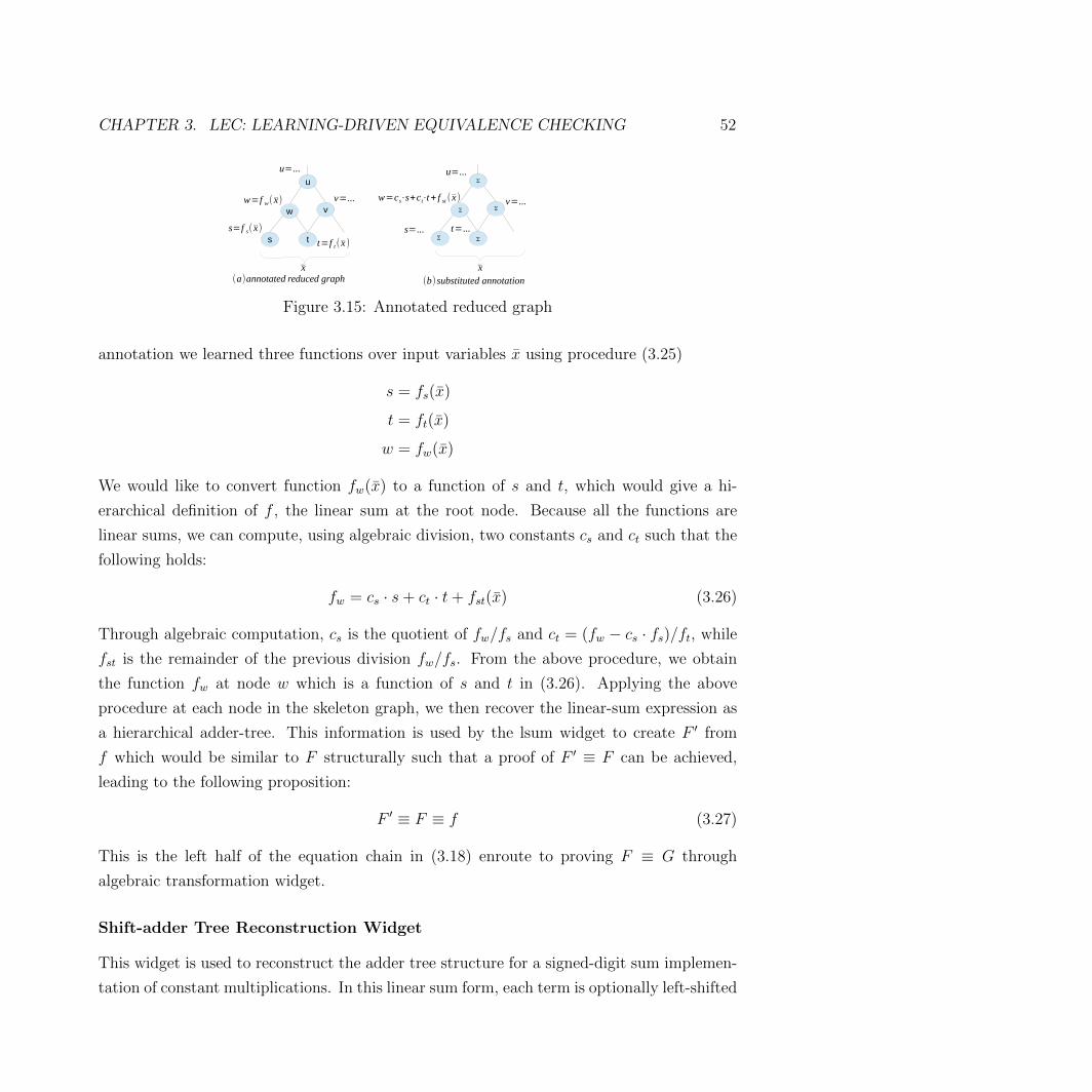
CHAPTER 3. LEC: LEARNING-DRIVEN EQUIVALENCE CHECKING 52
u
s t
vw
s=f s( x)
t=f t( x )
w=f w( x) v=...
u=...
s=... t=...
w=cs⋅s+ct⋅t+ f st ( x) v=...
u=...
(a)annotated reduced graph (b)substituted annotationx x
Σ
Σ
Σ
ΣΣ
Figure 3.15: Annotated reduced graph
annotation we learned three functions over input variables x using procedure (3.25)
s = fs(x)
t = ft(x)
w = fw(x)
We would like to convert function fw(x) to a function of s and t, which would give a hi-
erarchical definition of f , the linear sum at the root node. Because all the functions are
linear sums, we can compute, using algebraic division, two constants cs and ct such that the
following holds:
fw = cs · s+ ct · t+ fst(x) (3.26)
Through algebraic computation, cs is the quotient of fw/fs and ct = (fw − cs · fs)/ft, while
fst is the remainder of the previous division fw/fs. From the above procedure, we obtain
the function fw at node w which is a function of s and t in (3.26). Applying the above
procedure at each node in the skeleton graph, we then recover the linear-sum expression as
a hierarchical adder-tree. This information is used by the lsum widget to create F ′ from
f which would be similar to F structurally such that a proof of F ′ ≡ F can be achieved,
leading to the following proposition:
F ′ ≡ F ≡ f (3.27)
This is the left half of the equation chain in (3.18) enroute to proving F ≡ G through
algebraic transformation widget.
Shift-adder Tree Reconstruction Widget
This widget is used to reconstruct the adder tree structure for a signed-digit sum implemen-
tation of constant multiplications. In this linear sum form, each term is optionally left-shifted

CHAPTER 3. LEC: LEARNING-DRIVEN EQUIVALENCE CHECKING 53
before being added. For example, the logic in Figure 3.21 is implementing a linear sum of
the following form:
x55� 8 + (x46� 8 + (((x19� 4 + (x0 + x2� 1)) + x12� 4) + x32� 5))) (3.28)
The goal of this widget is to reconstruct the shift amount and order of additions, which can
not be extracted using the adder-tree reconstruction technique in Section 3.3. This widget
uses a specialized procedure that utilizes the structural information of concat and extract
operators to guess the amount of shifting before each adder node. In doing so, the shift-adder
tree structure is extracted from the original WNK network into a linear sum formula in the
form of (3.28). In the case-study of Section 3.5, an example of such an adder tree is shown
in Figure 3.21 and the reverse-engineered shift-adder tree linear-sum expressions are shown
in Figure 3.20.
The learning widgets, related to the above linear-sum, effectively reverse engineers the alge-
braic function of the underlying Boolean logic both functionally and structurally. Together
they allow the application of the algebraic-transformation widget, which effectively allows
LEC to reason beyond Boolean logic, taking on some of the power of a theorem prover.
3.4 System Integration: Proof-tree Infrastructure
Figure 3.16 shows the current solver and transformation widgets available in LEC. Because
transformation widgets produce sub-model lemmas as proof obligations, the LEC proof pro-
cess can be viewed as a spanning sub-model tree. The leaves of the tree are miter models
which are to be solved by solver widgets, returning a proof result of SAT, UNSAT, and
UNRESOLVED. Non-leaf nodes are marked with a lemma type from Table 3.2 during the
widget’s transformation. The lemma type indicates the inference rules used for the trans-
formation; the parent proof result is then calculated by applying the inference rule over
children’s proof results.
To propagate proof results from children to the parent node, all pre-lemma child nodes must
be proven UNSAT. Then, to calculate the proof-result from the rest of its immediate children,
s-lemma children are disjunctive as an UNSAT or SAT result is propagated to the parent
if any one of its s-lemma children is proven UNSAT or SAT respectively. The e-lemma is
conjunctive for an UNSAT result because it requires all e-lemma children to evaluate to

CHAPTER 3. LEC: LEARNING-DRIVEN EQUIVALENCE CHECKING 54
UNSAT, but disjunctive for a SAT result because only one of e-lemmas is required to be
proven SAT. The truth tables in Tables 3.5 and 3.6 reflect the above inference rules for a set
of s-lemmas and a set of e-lemmas.
To complete the truth table, the BOT value is used as the initial value for all nodes. To reflect
all possible truth table combinations, a CON value is used for when there is a conflict between
s-lemmas where one returns SAT and another returns UNSAT. This situation indicates there
is an internal software bug in LEC.
structural hashing
rewriting case-split
linear-sum construction
hier-sum
case0 case1 ...casen
M F=F 'MG=G '
pre-lemma0
pre-lemma1
...s-lemma
Verilog Miter Model
constant reduction
SolverWidgets
PEP pep0
pep1 ...
pepm
lsum ...
LEC
abstraction ...
Figure 3.16: Branching sub-model tree
‖ SAT UNS UNK CON BOTSAT SAT CON SAT CON SATUNS CON UNS UNS CON UNSUNK SAT UNS UNK CON UNKCON CON CON CON CON CONBOT SAT UNS UNK CON BOT
Table 3.5: Disjunctions of s-lemmas
& SAT UNS UNK CON BOTSAT SAT SAT SAT CON SATUNS SAT UNS UNK CON UNSUNK SAT UNK UNK CON UNKCON CON CON CON CON CONBOT SAT UNS UNK CON BOT
Table 3.6: Conjunction of e-lemmas
Using the truth tables and model trees, the status of a LEC proof can be evaluated at any
time to give a clear view of the proof progress. The proof log in Figure 3.17 is an example
sub-model spanning tree showing only the sub-tree that leads to the root’s UNSAT result.
The pre-lemma used along the path is not shown. Indentation indicates the parent-child

CHAPTER 3. LEC: LEARNING-DRIVEN EQUIVALENCE CHECKING 55
relationship. Recursively, the proof result of the top level target is evaluated as UNSAT
from the leaf nodes. In this proof log, the ’simplification’ node is a composite LEC widget
implementing a generic simplification procedure that repeatedly applies structural hashing,
constant identification and reduction, PEP identification and reduction widgets to simplify
the miter model. The decision for identifying constants, PEPs, abstraction cut-sets and
case-split patterns are obtained using the learning widgets.
{
"case split": {
"case_0": "UNSAT by AIG"
"case_1": {
"simplification": {
"abstraction": {
"case split": {
"case_00": "UNSAT by AIG",
"case_01": "UNSAT by AIG",
"case_10": "UNSAT by AIG",
"case_11": "UNSAT by AIG"
},
},
},
},
},
}
-------------------------------------
Miter proof result: [Resolved: UNSAT]
-------------------------------------
Figure 3.17: Illustration of proof log
Using the lemma annotated model-tree structure, LEC can be extended with new widgets or
composite widgets which combine existing widgets. Because the sibling nodes in the model
tree are independent of each other, all LEC widgets can be launched in parallel. The final
proof result is computed from the leaves and the use of the pre-lemma guarantees that only
valid transformations contribute to the root’s proof result, which guarantees the correctness
of LEC’s proof.

CHAPTER 3. LEC: LEARNING-DRIVEN EQUIVALENCE CHECKING 56
3.5 Case Studies
Image Processing Design
The first case-study is an industrial example taken from the image processing application
area. We verify specification = implementation where the “specification” is a manually-
specified high-level description of the design. “Implementation” is a machine-generated
highly-optimized RTL implementation of the same design using a high-level synthesis (HLS)
tool like [14]. The miter logic is obtained through SLEC [15], a commercial C-to-Verilog
equivalence checking tool. The miter problem is to verify that the HLS tool did not modify
the design’s behavior.
This miter was sequential in nature, but here we examine a related bounded model checking
(BMC) problem which checks the correctness of the implementation at cycle N. This renders
the problem combinational. This is relevant because the sequential problem in this case is
too hard to solve in general, and even the BMC problem at cycle N was too difficult for
industrial tools.
The original design (specification) consists of 150 lines of C++. This was processed with the
Calypto front end [15] and was synthesized into a word-level Verilog netlist. The generated
miter model had 1090 lines of structural Verilog code with 36 input ports: 29 of which are
7 bits wide, 2 are 9 bits, 4 are 28 bits and one is a single-bit wire. The miter is comparing
two 28-bit output values. We do not have knowledge about the design intent except through
structural statistics: no multipliers, many adders, subtractors, comparators, shifters etc.,
together with Boolean logic. From a schematic produced from the Verilog, there seems to
be a sorting network implemented using comparators, but we could not deduce anything
further.
Figure 3.18 illustrates the compositional proof produced by LEC and shows the sub-model
tree created during the proof process. The major steps it went through are case-split, simpli-
fication, abstraction, PEP transformation and linear-reconstruction. Indentations indicating
parent and sub-model relations are listed in the order they were created. The three numbers
on the right are the node counts in the red, blue and purple regions (common logic) of the
WNK network as distinguished in Figure 3.12(a) which in this cases-study is an indication
of the progress. Only those sub-models that contributed to the final proof are shown in the
figure. Others are ignored because the sub-models, which were kept, are sufficient to obtain

CHAPTER 3. LEC: LEARNING-DRIVEN EQUIVALENCE CHECKING 57
the UNSAT result for the root model.
1.original model : 366 332 776
2. case-split
3. case_0 : 366 331 844
4. simplification :
5. AIG solver : UNSAT
6. case_1 : 366 332 776
7. simplification : 344 289 675
8. abstraction : 344 289 29
9. case-split
10. case_0 : 344 289 31
11. AIG solver : UNSAT
12. case_1 : 344 289 31
13. simplification : 343 288 27
14. PEP-reduction
15. pep_0 : 335 280 27
16. linear sum re-construction
17. pre-lemma
18. f=g : UNSAT
19. pre-lemma_F=F'
20. AIG solver : UNSAT
21. pre-lemma_G=G'
22. AIG solver : UNSAT
23. s-lemma
24. simplification : 10 10 305
25. AIG solver : UNSAT
Figure 3.18: Sub-model proof tree
As seen in Figure 3.18, the case-split procedure is applied twice, at lines 2 and 9. Both models
have a single-bit input port, which was selected for cofactoring. ABC [2] immediately proves
the first case-split case, case 0 (line 3 and 10) , using SAT sweeping on the AIG model at
line 5 and 11 using ABC’s dcec [52] with a time-out of two seconds. The abstraction widget
was applied at line 8, reducing the common logic (purple) from 675 to 29 WNK nodes. This
happens to remove all the comparator logic. The case-split procedure applied at line 2 is
important; we tried abstraction on the original model (at line 1) directly, but it failed to
produce a useful abstracted sub-model.
Model 15 is the smallest unproved PEP from model 13. It is proven using the linear sum
re-construction widget at line 16, which we will describe in more detail below. Model 23 is

CHAPTER 3. LEC: LEARNING-DRIVEN EQUIVALENCE CHECKING 58
the s-lemma after merging pep0 in the PEP-reduction transformation step at line 15.
After simplification at line 24, most of the post pep0- merging logic in model 23 (red and blue)
became common logic(purple) through structural hashing, leaving only 10 nodes in each of
the blue and red regions. Model 25 was proved quickly by ABC which concludes the proof
of the original miter at the root of the model-tree. In this case, the linear re-construction
procedure was crucial in attaining the proof. However, the case-split, simplification, abstrac-
tion, and PEP transformations are necessary enabling steps leading to the applicability of
the linear sum transformation widget for model 15.
Linear Sum Re-construction
For model 15 in Figure 3.18, the WNK network contains many +,−, � and � operators
along with extract and concat operators, but contains no Boolean operators or muxes. This
is an indication that the WNK is likely implementing a pure algebraic function. The input
ports consist of twenty-five 7-bit or 12-bit wide ports. The miter is comparing two 15-bit
wide output ports. At this point, simplification and abstraction can not simplify the model
further. Also, there are no good candidates for case-splitting. The local rewriting rules can
not be applied effectively without having some global information to help converge the two
sides of the miter logic. High-level information must be extracted and applied to prove this
miter model.
The linear sum learning widget shows the following linear sum function is found on both
sides of the miter logic:
−16 ∗ x0 + 2 ∗ x1 + 2 ∗ x2 + 2 ∗ x3 + 2 ∗ x4 + 2 ∗ x5 + 2 ∗ x6 + 2 ∗ x7 + 2 ∗ x7 + 2 ∗ x8 + 2 ∗ x9
+2 ∗ x10 + x11 + x12 + 2 ∗ x13 + 2 ∗ x14 + 2 ∗ x15 + 2 ∗ x16 + 2 ∗ x17 + 2 ∗ x18 + 2 ∗ x19
−2 ∗ x20 + 2 ∗ x21 + 2 ∗ x22 + 2 ∗ x23 + 2 ∗ x24 + 14
Then the adder-tree-reconstruction widget returns that one side of the miter implements
the above sum as a plain linear adder chain Figure 3.19(a), the other side is a highly op-
timized implementation using a balanced binary tree structure (Figure 3.19(b)) and using
optimization tricks, which we don’t fully understand.

CHAPTER 3. LEC: LEARNING-DRIVEN EQUIVALENCE CHECKING 59
(a)linear adder chain (b)balanced adder tree
...
...
Figure 3.19: Addition implementation
The above learning results allow the linear-sum transformation widget to proceed and create
the lemmas as in Figure 3.11, which lead to the final UNSAT result at the root node.
A More Complex Adder-Tree
The sub-model lemma tree of the second case-study is shown in Figure 3.20. In this example,
we use xi to denote a node in the miter network MM at each sub-model node. LEC applies
the learning widgets to identify sub-graphs rooted at node xi which are implementing linear
sum functions and transforms them using lsum2 or hier-lsum widgets. At a high level, the
design under comparison has a sub-graph which adds four constant multiplications of 17-bit
signed-integers functionally:
181 · x1 − 181 · x18 − 181 · x33 + 181 · x4 (3.29)
where x1, x18, x33 and x4 are the input nodes to the subgraph in MM .
LEC’s proof steps are shown in Figure 3.20 as a spanning sub-model tree. In getting the LEC
proof, LEC’s learning widgets are able to reveal in great detail how these numbers are added
in the circuit. For the miter network model at each sub-model tree node, lemmai indicates
that a subgraph rooted at node xi is identified as a linear sum; the reverse engineered formula
is shown on the right side. For example, at line 23, lemma161 and the learned expression
x101 + 2 ∗ x107 + 16 ∗ x116 + 16 ∗ x122 + 32 ∗ x135 + 256 ∗ x148 + 256 ∗ x156 (3.30)
shows the subgraph rooted at node x161 and bounded by nodes x101, x107, x116, x122, x135,
x148, and x156 is implementing the formula (3.30). Similarly, at line 17, node x135 is identified
as 2 · x32 + 1.

CHAPTER 3. LEC: LEARNING-DRIVEN EQUIVALENCE CHECKING 60
0 root UNSAT <- ['simplification']1 simplification UNSAT <- ['abstraction']2 abstraction UNSAT <- ['simplification']3 simplification UNSAT <- ['lsum2 ']
4 lsum2 UNSAT <- all sub-model UNSAT5 lemma_212 UNSAT <- ['linear_construction']# 362*x1-362*x18-362*x33+362*x46 linear_construction UNSAT <- all sub-model UNSAT7 lemma_F=F' UNSAT <- ['simplification']8 simplification UNSAT <- ['dcec']9 lemma_G=G' UNSAT <- ['dcec']10 lemma_166 UNSAT <- ['hier-lsum'] # 181*x1-181*x18-181*x33+181*x411 hier-lsum UNSAT <- all sub-model UNSAT12 lemma_0 UNSAT <- ['dcec'] # x013 lemma_51 UNSAT <- ['dcec'] # x5014 lemma_2 UNSAT <- ['dcec'] # x015 lemma_3 UNSAT <- ['dcec'] # x316 lemma_5 UNSAT <- ['dcec'] # x317 lemma_135 UNSAT <- ['dcec'] # 2*x32+118 lemma_10 UNSAT <- ['dcec'] # x819 lemma_17 UNSAT <- ['dcec'] # x1720 lemma_18 UNSAT <- ['dcec'] # -x17-121 lemma_20 UNSAT <- ['dcec'] # x1822 lemma_32 UNSAT <- ['dcec'] # x3223 lemma_161 UNSAT <- ['simplification'] # x101+2*x107+16*x116+16*x122+32*x135+256*x148+256*x156
24 simplification UNSAT <- ['adder-shift-tree']25 adder-shift-tree UNSAT <- all sub-model UNSAT26 lemma_64 UNSAT <- ['dcec'] # (x55*256+(x46*256+(((x19*16+(x0+x2*2))+x12*16)+x32*32)))27 s-lemma UNSAT <- ['linear_construction']28 linear_construction UNSAT <- all sub-model UNSAT29 lemma_F=F' UNSAT <- ['dcec']30 lemma_G=G' UNSAT <- ['dcec']31 lemma_34 UNSAT <- ['dcec'] # 2*x32+132 lemma_163 UNSAT <- ['dcec'] # x161+x8233 lemma_165 UNSAT <- ['dcec'] # x16434 lemma_166 UNSAT <- ['dcec'] # x16535 lemma_42 UNSAT <- ['dcec'] # -x0-136 lemma_171 UNSAT <- ['dcec'] # x037 lemma_44 UNSAT <- ['dcec'] # x4238 lemma_45 UNSAT <- ['dcec'] # -x3-139 lemma_174 UNSAT <- ['dcec'] # x340 lemma_47 UNSAT <- ['dcec'] # x4541 lemma_49 UNSAT <- ['dcec'] # x44+x4742 lemma_179 UNSAT <- ['dcec'] # x3243 lemma_180 UNSAT <- ['dcec'] # -x17944 lemma_181 UNSAT <- ['dcec'] # x18045 lemma_186 UNSAT <- ['dcec'] # x1746 lemma_187 UNSAT <- ['dcec'] # -x18647 lemma_188 UNSAT <- ['dcec'] # x18748 lemma_190 UNSAT <- ['dcec'] # x181+x18849 lemma_193 UNSAT <- ['dcec'] # x174+x19150 lemma_196 UNSAT <- ['dcec'] # x171+x19451 lemma_198 UNSAT <- ['dcec'] # 181*x19752 lemma_199 UNSAT <- ['dcec'] # x19853 lemma_200 UNSAT <- ['dcec'] # x19954 lemma_73 UNSAT <- ['dcec'] # 2*x71+155 lemma_82 UNSAT <- ['adder-shift-tree'] # 4*x12+4*x20+8*x34+64*x53+64*x59+128*x73+x8
56 adder-shift-tree UNSAT <- all sub-model UNSAT57 lemma_68 UNSAT <- ['dcec'] # (((x38*64+(((x8*4+x0)+x2*4)+x21*8))+x31*64)+x51*128)58 s-lemma UNSAT <- ['linear_construction']59 linear_construction UNSAT <- all sub-model UNSAT60 lemma_F=F' UNSAT <- ['dcec']61 lemma_G=G' UNSAT <- ['dcec']62 lemma_85 UNSAT <- ['dcec'] # x7163 lemma_7 UNSAT <- ['dcec'] # x2+x564 lemma_71 UNSAT <- ['dcec'] # -x32-165 lemma_98 UNSAT <- ['dcec'] # -x17+51166 lemma_59 UNSAT <- ['dcec'] # x1767 lemma_100 UNSAT <- ['dcec'] # x85+x9868 lemma_107 UNSAT <- ['dcec'] # 2*x71+169 lemma_148 UNSAT <- ['dcec'] # x1870 lemma_122 UNSAT <- ['dcec'] # x1771 s-lemma UNSAT <- ['linear_construction'] # None72 linear_construction UNSAT <- all sub-model UNSAT73 lemma_F=G' UNSAT <- ['dcec']74 lemma_G=G' UNSAT <- ['dcec']75 s-lemma UNSAT <- ['dcec'] # None
Figure 3.20: Proof log

CHAPTER 3. LEC: LEARNING-DRIVEN EQUIVALENCE CHECKING 61
From the sub-model tree, widget lsum2 is applied to line 4 over lemma 212 (line 5) and
lemma 166 (line 10) which are identified as top-level linear sums:
lemma 212@line5 : 362 ∗ x1− 362 ∗ x18− 362 ∗ x33 + 362 ∗ x4 (3.31)
lemma 166@line10 : 181 ∗ x1− 181 ∗ x18− 181 ∗ x33 + 181 ∗ x4 (3.32)
and hier-lsum widget is applied at line 11.
Lemma 212 is proven quickly using the linear sum construction widget at line 6, while
Lemma 166 is more complex because it internally contains many sub-graph adder trees
(hier-lsum widget applicable) and two adder-shift trees at lines 23 and 56 with the following
linear sum expressions:
lemma 64@line26 : (x55 ∗ 256 + (x46 ∗ 256 + (((x19 ∗ 16 + (x0 + x2 ∗ 2)) + x12 ∗ 16) + x32 ∗ 32)))
(3.33)
lemma 68@line57 : (((x38 ∗ 64 + (((x8 ∗ 4 + x0) + x2 ∗ 4) + x21 ∗ 8)) + x31 ∗ 64) + x51 ∗ 128)
(3.34)
Both are specific adder-shift adder trees because all the coefficients are powers of 2. Figure
3.21 is the actual WNK network for the adder-shift tree for lemma 64 @line26. It is rather
surprising to learn that such a complex logic network is a simple linear sum function. Once
the adder-shift tree is discovered, the algebraic transformation widget is then applied to
establishe the proof through the chain of equations: F ′ ≡ F ≡ f ≡ g ≡ G ≡ G′.
In this case study, the iterative applications of LEC learning and transformation widgets
allow a very detailed reverse-engineering of the underlying linear sum formula that was
implemented. In order to establish a proof using algebraic reasoning, both the functional
and structural information of the linear sum formula are identified which are crucial in
establishing LEC’s proof.
3.6 Experimental Results
Table 3.7 shows the experimental results comparing Boolector [13], Z3 [23] and iprove [52]
using a 24-hour time-out limit on a 2.6 Ghz Intel Xeon processor. These models are generated
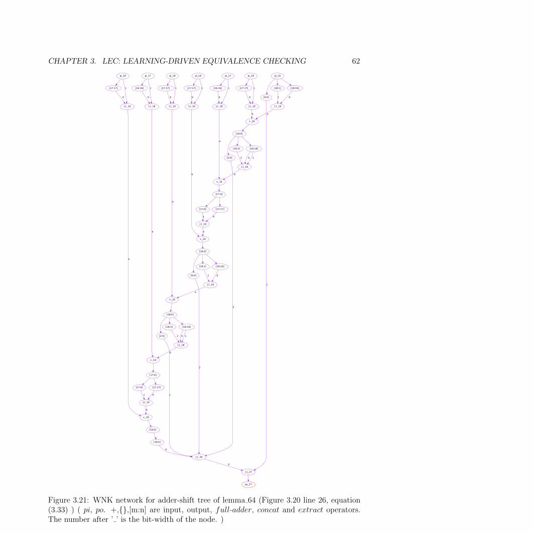
CHAPTER 3. LEC: LEARNING-DRIVEN EQUIVALENCE CHECKING 62
[0:0]
{}_27
1
pi_19
[18:1] [18:18]
pi_18
[17:17]
{}_19
1
pi_18
[17:17]
{}_19
1
pi_17
[16:16]
{}_18
1
pi_18
[17:17]
{}_19
1
pi_17
[16:16]
{}_18
1
pi_18
[17:17]
{}_19
1
0
po_27
+_20
b
{}_19
1 0
a
[18:0]
[2:0]
[18:3] [18:18]
{}_26
3
0
+_20
b
{}_18
2 0 1
+_19
b
0
a
[17:0]
[17:0] [17:17]
{}_19
1 0
a
[18:0]
[0:0]
[18:1] [18:18]
2
0
+_20
b
{}_19
1 0
a
[18:0]
[2:0]
[18:3] [18:18]
1
{}_18
2 0 1
+_19
b
0
a
[17:0]
[17:0] [17:17]
{}_19
1 0
+_20
b
0
a
[18:0]
[18:0]
0
0
Figure 3.21: WNK network for adder-shift tree of lemma 64 (Figure 3.20 line 26, equation(3.33) ) ( pi, po. +,{},[m:n] are input, output, full-adder, concat and extract operators.The number after ’ ’ is the bit-width of the node. )

CHAPTER 3. LEC: LEARNING-DRIVEN EQUIVALENCE CHECKING 63
directly using SLEC [15] for checking C-to-RTL equivalence or extracted as a sub-target from
PEPs. The first column is the miter design name. The second column is the number of lines
of Verilog for the miter model specification. Run-time or time-out results are reported for
each solver in columns 3 to 6. Although the miter models are not large in terms of lines of
Verilog, they are quite challenging for Boolector, Z3 and iprove. The run-time of LEC is
the total CPU time including Verilog compilation. It was expected that iprove would not
prove any of these designs because it works on the bit-blasted model without any high-level
information which the other solvers have.
Design Lines Boolector z3 iprove LECmul 64 64 125 20 sec 200 sec timeout 10 sec
d1 24 time-out time-out time-out 15 secd2 507 time-out time-out time-out 2 mind3 191 time-out time-out time-out 15 mind4 473 time-out time-out time-out 1 min
d5 case 1 1090 time-out time-out time-out 10 mind5 case 1 pep 0 674 time-out 9 hour time-out 4 min
d6 case 2 205 time-out time-out time-out 10 min
Table 3.7: Benchmark comparison (Timeout 24 hours)
The miter, mul 64 64, compares a 64x64 multiplier in the LHS with an implementation using
four 32x32 multipliers using the following equation:
{aH , aL} · {bH , bL} = (aH · bH)� 64 + (aH · bL + aL · bH)� 32 + aL · bL
where aH , aL, bH , bL are the 32-bit slices of the original 64-bit bit-vectors. Both Boolector
and Z3 are able to prove it. LEC proves it by first utilizing rewriting rules to transform the
64x64 multiplier into four 32x32 multipliers, matching the other four in the RHS of the miter.
Because they are matched exactly, they become common logic in the miter model. LEC then
produces an abstraction and obtains a reduced model with all the multipliers removed: the
outputs of the multipliers become free inputs in the abstract model. The abstract model is
then proven instantly by ABC’s ”dcec” algorithm on the AIG model.
Miter d1, extracted from a PEP sub-model, is a demonstration of rewrite Rule 6 (distribution
of multiplication over concat operator) in Table 3.3 using 32-bit multiplication. As both
Boolector and Z3 fail to prove equivalence within the time-limit, they likely do not have this
rewriting rule implemented.

CHAPTER 3. LEC: LEARNING-DRIVEN EQUIVALENCE CHECKING 64
To prove d2, LEC executes a conditional rewriting using rule (3.8) by first statically proving
an invariant in the form of (3.9). After the transformation, the multipliers are matched
exactly on both sides of the miter and removed in the subsequent abstract model. The final
miter model is proved instantly by ABC on the bit level AIG.
The miter model d3 has part of its logic that is similar to mul 64 64 embedded inside. LEC
proves d3 by first applying rewriting rules repeatedly until no more rewriting is possible.
Then, LEC computes a reduced model through abstraction. In the reduced model, LEC
executes a case-split on a one-bit input. The case-0 AIG model is proven instantly, while
case-1 is proven in about 10 minutes by ABC.
Miter d4 is proven by first executing a case-split of two bit-vector inputs. Three of the four
co-factored cases are proven instantly. The one that is unresolved goes through a round of
simplification and abstraction. On the resulting sub-model, three one-bit inputs are identified
and co-factored through case-split procedures. LEC proves all resulting eight cases within a
few seconds.
Miter d5 case 1 is the top-level model presented in the first case study in Section 3.5. LEC
completes the proof in 10 minutes while all other solvers time out. Miter d5 case 1 pep 0 is
extracted from this miter model at line 15 in Figure 3.18, which is the linear sum miter. For
this simpler miter, Z3 is able to prove it in 9 hours while both iprove and Boolector time
out. This shows that by using collaborating procedures through simplification, abstraction
and case-split widgets, LEC’s transformations successfully reduce the surrounding logic in
the original model, which was preventing Z3 from proving it in 24 hours.
Miter d6 case 2 is the top-level model presented in the second case-study in Section 3.5.
Figure 3.20 shows the procedures that lead to the proof. The overall run-time for LEC is 10
minutes, while all three other solvers time out.
The above experiments demonstrate the effectiveness of LEC’s collaborating procedures of
simplification, rewriting, case-splitting and abstraction computations. The LEC architec-
ture allows these procedures to be applied recursively through a sub-model tree: the model
obtained by one widget introduces new opportunities for applying other widgets in the next
iteration. As exemplified in Miter d4, the initial case-split gives rise to new opportunities for
simplification as new constants are introduced by cofactoring. Then a new round of abstrac-
tion is able to remove enough common logic and expose three one-bit inputs as case-split

CHAPTER 3. LEC: LEARNING-DRIVEN EQUIVALENCE CHECKING 65
candidates in the reduced model, which in turn gives rise to another case-split transforma-
tion that leads to the final proof. None of this seems possible without the transformations
being applied in sequence.
3.7 Comparison with Related Work
In bit-level equivalence-checking procedures [42] [52] [55], simulation, SAT-sweeping, AIG
rewriting and internal equivalence identification are all relevant to data-path equivalence-
checking. In LEC, these types of procedures are conducted at the word-level. Word-level
rewriting is difficult if only a bit-level model is available. For example, with no knowledge
of the boundary of a multiplier, normalizing its operands is impractical at the bit-level .
Although abstraction and case-split techniques in LEC can be applied at the bit-level in
theory, these are not used due to the difficulty of computing an abstraction boundary or of
finding good cofactoring candidates.
SMT solving is relevant because a data-path is a subset of QF BV theory. Methods such as
[4] [13] [23] [18] [24] [34], are state-of-art QF BV solvers. These employ different implementa-
tions of word-level techniques in rewriting, abstraction, case-splitting, and simplification, and
interleave Boolean and word-level reasoning via a generalized DPLL framework or through
abstraction refinements of various forms. In our experience, the SMT solvers are very efficient
on SAT instances.
Hector[38] is closest to LEC in terms of technology and targeted application domains, and
has a rich set of word-level rewriting rules along with some theorem prover [4] procedures
to validate every rewriting applied. Hector also has an orchestration of a set of bit-level
solvers using SAT and BDD engines to employ once the bit-level miter model is constructed.
Strategically, LEC relies less on the capacity of a SAT solver and instead builds a composi-
tional proof infrastructure and employs iterative transformations to obtain a proof through
sub-model trees.
The techniques in [56] [62] [68] also try to reconstruct an algebraic model from the underlying
logic, but they employ a bottom up approach and their primitive element is a half-adder.
The method in [5] simplifies the algebraic construction by solving an integer linear pro-
gramming problem. The limitation of these approaches is that they rely on the structural
pattern of the underlying logic to reconstruct the algebraic model. On the other hand, the

CHAPTER 3. LEC: LEARNING-DRIVEN EQUIVALENCE CHECKING 66
linear construction case-study in Section 3.5 constructs the polynomial through probing with
simulation patterns. This is more general as it uses only the functional information of the
data-path logic. For different domains, other techniques may well be more applicable such as
the bottom-up approach. The use of vanishing polynomials and Grobner bases in [57][58] to
prove equivalence between polynomials in the modulo integer domain can be utilized once a
polynomial form is reconstructed in LEC. However, in many data-path miter models, such a
polynomial in a certain domain or theory is likely embedded in other control and data-path
logic. Direct application of algebraic techniques is often not practical. Thus the collaborat-
ing procedures in LEC are designed to bridge this gap and isolate such polynomials so that
these high level theories can then be applied.
Recent developments in [47] [46] try to recognize high-level constructs from a bit-level sequen-
tial network, while LEC establishes linear-sum relationships using functional and structural
information of the WNK word level network. The work in [44] tries to reconstruct the
factored form for constant-coefficient multiplication using partial products at the bit-level,
while our method is effective at the word-level WNK network. In conducting consistency
checking between C and Verilog RTL, the work [39] focuses on how to process a C program
to generate formal models. The tool relies on SMT solvers [13] [18] [23] as the back-end
solving engines.
Clearly, LEC is not a theorem prover, however, there is some similarity at the high-level
view. Both require design knowledge in order to reason beyond Boolean logic. Using first
order logic, a theorem prover is expressive enough and very rigorous in reasoning between the
Boolean and algebraic domains. However, LEC uses an Algebraic-to-Boolean procedure to
covert an algebraic expression into Boolean logic. Also, LEC is more applicable and easier
to use as it works on general RTL directly, using learning and transformation widgets to
unravel the underlying algebraic function.
In terms of tool architecture, [6] [12] [41], all employ a sophisticated set of transformations
to simplify the target model during verification. These are done at the bit-level. The
LEC infrastructure allows future extension to take advantage of multi-core parallelization as
demonstrated in [61]. Methods in [17] and [66], use dedicated data-structures to represent
the proof-obligations, while LEC relies on the sub-model tree to track the compositional
proof strategy used at each node.

CHAPTER 3. LEC: LEARNING-DRIVEN EQUIVALENCE CHECKING 67
3.8 Conclusion
In LEC, we designed and implemented a system of collaborating procedures for data-path
equivalence-checking problems found in industrial settings. The strategy is to utilize Boolean-
level solvers, conduct transformations at the word-level and to synthesize internal similarities
by lifting the reasoning to the algebraic level. Using real industrial case-studies, we demon-
strated with LEC the applicability of the sub-tree infrastructure for integrating a composi-
tional proof methodology, LEC was able to prove problems within a few minutes that were
unsolved in 24 hours by three other competing methods.

68
Chapter 4
A Simple Trusted Translation
Procedure from C to Verilog
Simplicity is the prerequisite of
reliability.
Edsger Dijstra
Make things as simple as
possible, but not simpler.
Albert Einstein
The objective of this chapter has two goals:
1. Build a simple trusted translator from C programs to a hardware description language
(in this case Verilog).
2. Apply this to the formal verification of hardware and software systems using highly
developed hardware model checking systems and methods.
In combination, these comprise a C-based model checker.

CHAPTER 4. A SIMPLE TRUSTED TRANSLATION PROCEDURE FROM C TOVERILOG 69
To achieve the first goal, we used the LLVM compiler infrastructure [45] to compile C
programs into LLVM Bytecode, and used a straightforward method to translate these into
Verilog circuits. The implementation is able to handle most C constructs, including some
problematic ones such as arbitrary loops and static array access.
For the second goal, both equivalence checking and property checking will be illustrated.
For equivalence checking, related IEEE 754 [32] compliant floating point units (FPUs) were
compared; namely OpenCores VHDL or Verilog hardware models were compared with related
C-coded SoftFloat versions [30]. Interestingly, this revealed several bugs in the OpenCores
hardware models. For model checking safety properties, benchmarks from the 2015 Software
Verification Competition were examined. This also revealed discrepancies with some of the
expected results (truth values), assigned by the competition committee, with the correct
results. In both situations, counterexamples were generated and cross-checked against the
original C-program to validate their correctness.
4.1 Introduction
In the previous chapter, some very difficult equivalence checking problems were tackled,
where different Verilog word-level models were compared for combinational equivalence. In
this chapter, we move up a level of initial description to the C language and address an
increasingly popular way of designing hardware, using software specifications. We also look
at the verification of software directly.
This work was motivated by a growing interest in reasoning about and proving properties
specifically about C software programs. C is also of increasing interest in the hardware
domain, where C is used as a hardware specification language. While the actual implemented
hardware is typically described in Verilog and synthesized from that, it is the C model that
is usually certified by massive simulations. In this sense, the C model represents the golden
model and is used to compare against a related Verilog model using equivalence checking.
This requires a highly trusted translation from C to Verilog to create a golden Verilog model
for comparing against the Verilog implementation model used by the designers.
In the software domain, formally verifying a program against a set of properties has been
a subject of interest and active research for many years. Great strides have been made in
formal verification of both hardware and software. Our aim here is to bring the state-of-the-

CHAPTER 4. A SIMPLE TRUSTED TRANSLATION PROCEDURE FROM C TOVERILOG 70
art in hardware verification to the software domain and take advantage of advances made in
hardware verification methods.
We first focus on creating a translation tool that is as simple as possible using trusted
and well established intermediate tools to accomplish the task. We eschew optimization of
the generated Verilog model which can add complications and therefore can increase the
potential for introducing bugs. This allows existing hardware formal verification flows such
as equivalence and property checking of safety and liveness properties to be applied readily,
with a very high confidence that the translation process has not corrupted the golden model
and therefore the results can be trusted.
We use the LLVM compiler infrastructure and a straight-forward translation of its produced
LLVM Bytecode to create a Verilog program from a single thread C program. At this point,
an equivalence-checking Verilog (miter) model can be created comparing the actual hardware
model used for implementation with the synthesized-from-C model. Figure 4.1 shows the
high-level C-to-Verilog translation flow and how it fits into a C-to-RTL equivalence checking
methodology using hardware verification methods. Such a flow can also be used in the
software verification of C programs where C assert statements are translated into System
Verilog Assertions [1] (SVA) and compiled into logic using, for example Verific[64].
LLVM Bytecode
C C Model
Sequential equivalencechecking
Trace replay and debug
Verilog ModelVerilog Model
¿CVerilog Model
C = RTL ?
Figure 4.1: C vs RTL equivalence checking
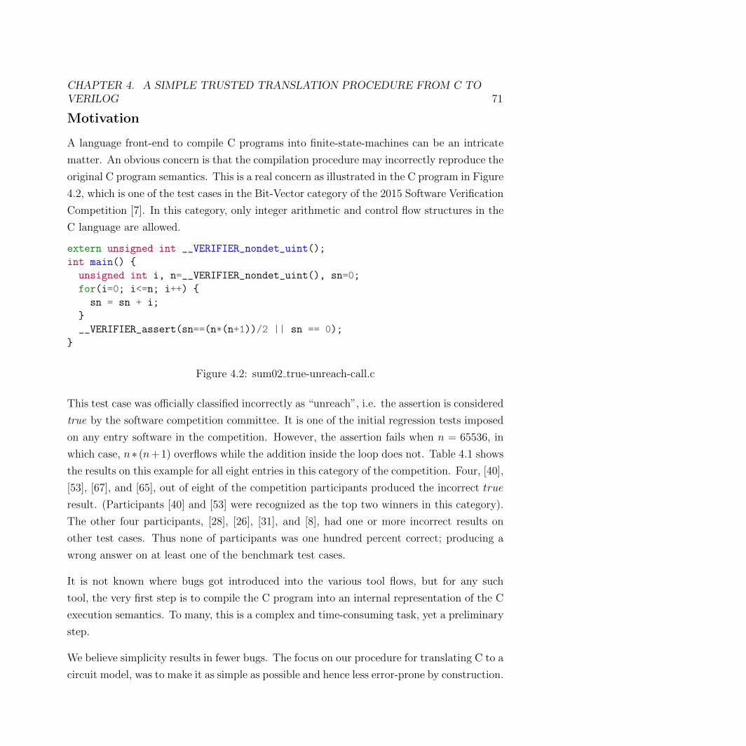
CHAPTER 4. A SIMPLE TRUSTED TRANSLATION PROCEDURE FROM C TOVERILOG 71
Motivation
A language front-end to compile C programs into finite-state-machines can be an intricate
matter. An obvious concern is that the compilation procedure may incorrectly reproduce the
original C program semantics. This is a real concern as illustrated in the C program in Figure
4.2, which is one of the test cases in the Bit-Vector category of the 2015 Software Verification
Competition [7]. In this category, only integer arithmetic and control flow structures in the
C language are allowed.
extern unsigned int __VERIFIER_nondet_uint();
int main() {
unsigned int i, n=__VERIFIER_nondet_uint(), sn=0;
for(i=0; i<=n; i++) {
sn = sn + i;
}
__VERIFIER_assert(sn==(n*(n+1))/2 || sn == 0);
}
Figure 4.2: sum02 true-unreach-call.c
This test case was officially classified incorrectly as “unreach”, i.e. the assertion is considered
true by the software competition committee. It is one of the initial regression tests imposed
on any entry software in the competition. However, the assertion fails when n = 65536, in
which case, n∗ (n+1) overflows while the addition inside the loop does not. Table 4.1 shows
the results on this example for all eight entries in this category of the competition. Four, [40],
[53], [67], and [65], out of eight of the competition participants produced the incorrect true
result. (Participants [40] and [53] were recognized as the top two winners in this category).
The other four participants, [28], [26], [31], and [8], had one or more incorrect results on
other test cases. Thus none of participants was one hundred percent correct; producing a
wrong answer on at least one of the benchmark test cases.
It is not known where bugs got introduced into the various tool flows, but for any such
tool, the very first step is to compile the C program into an internal representation of the C
execution semantics. To many, this is a complex and time-consuming task, yet a preliminary
step.
We believe simplicity results in fewer bugs. The focus on our procedure for translating C to a
circuit model, was to make it as simple as possible and hence less error-prone by construction.

CHAPTER 4. A SIMPLE TRUSTED TRANSLATION PROCEDURE FROM C TOVERILOG 72
Solvers Rank Consistency #Errors
ESBMC[53] 1st Buggy 1
CBMC[40] 2nd Buggy 1
CPAChecker[8] 3rd Buggy 1
Beagle 1.1[65] Buggy 1
Cascade 2.0[67] Buggy 1
Seahorn[28] Buggy > 1
Ultimate Automizer [31] Buggy > 1
Ultimate Kojak[26] Buggy > 1
Table 4.1: 2015 Software Verification Competition: Bit-Vector category
Our simple/trusted C-to-Verilog compilation should take the translation procedure out of
the verification equation, and reliably bridge the gap between software and hardware. This
allows existing hardware synthesis and verification techniques to be applied reliably in the
software domain.
Why Verilog
Verilog was chosen as the intermediate representation for the circuit model for the following
reasons:
• It is almost the industrial de facto standard for hardware description from which hard-
ware is synthesized and verified.
• Verilog’s always ff and always comb blocks can be used to express a finite state machine
model as sequential and combinational logic respectively.
• Verilog has been precisely defined by IEEE standards. Its well-defined syntax and
semantics make it easier to map the C semantics into Verilog constructs.
• Synthesis, simulation, emulation, validation and verification tool flows for Verilog can
be utilized readily after the translation.
• Validation of the translation procedure can be conducted by simulating the Verilog
model and comparing against the C-code program using random input vectors. In our
case, we used Verilator[60] to compile the generated Verilog code back to C++ to be
simulated.

CHAPTER 4. A SIMPLE TRUSTED TRANSLATION PROCEDURE FROM C TOVERILOG 73
• Verilog has sufficient constructs to capture all the original C constructs. This is im-
portant for retaining the original control flow and word-level operators after the trans-
lation.
A constraint imposed by the Verilog language is that the computation resources must be
statically resolvable at synthesis time. In contrast, C programs support dynamic resource
management such as memory allocation/de-allocation, run-time function call-stacks and run-
time parallel threads. Therefore, in this work, we limit the scope of translating from single-
thread C programs with arbitrary control flows, without those dynamic resource management
features.
Main Contributions
1. A simple procedure is presented, based on the LLVM compiler infrastructure, in which
a subset of C (excluding dynamic memory management, recursive functions and par-
allelism), can be mapped into a Verilog module using the always ff and always comb
blocks.
2. Experiments demonstrating C-to-RTL equivalence checking and software property check-
ing, show that such a flow allows existing hardware verification tool chains to be used,
producing promising results. The results also indicate that our flow is more reliable
than existing methods available.
Organization
C Function
?
SSA Representation(LLVM Bytecode)
?
Verilog Module
?
Logic Network
?
Finite State Machine
Figure 4.3: C-to-Verilog Translation
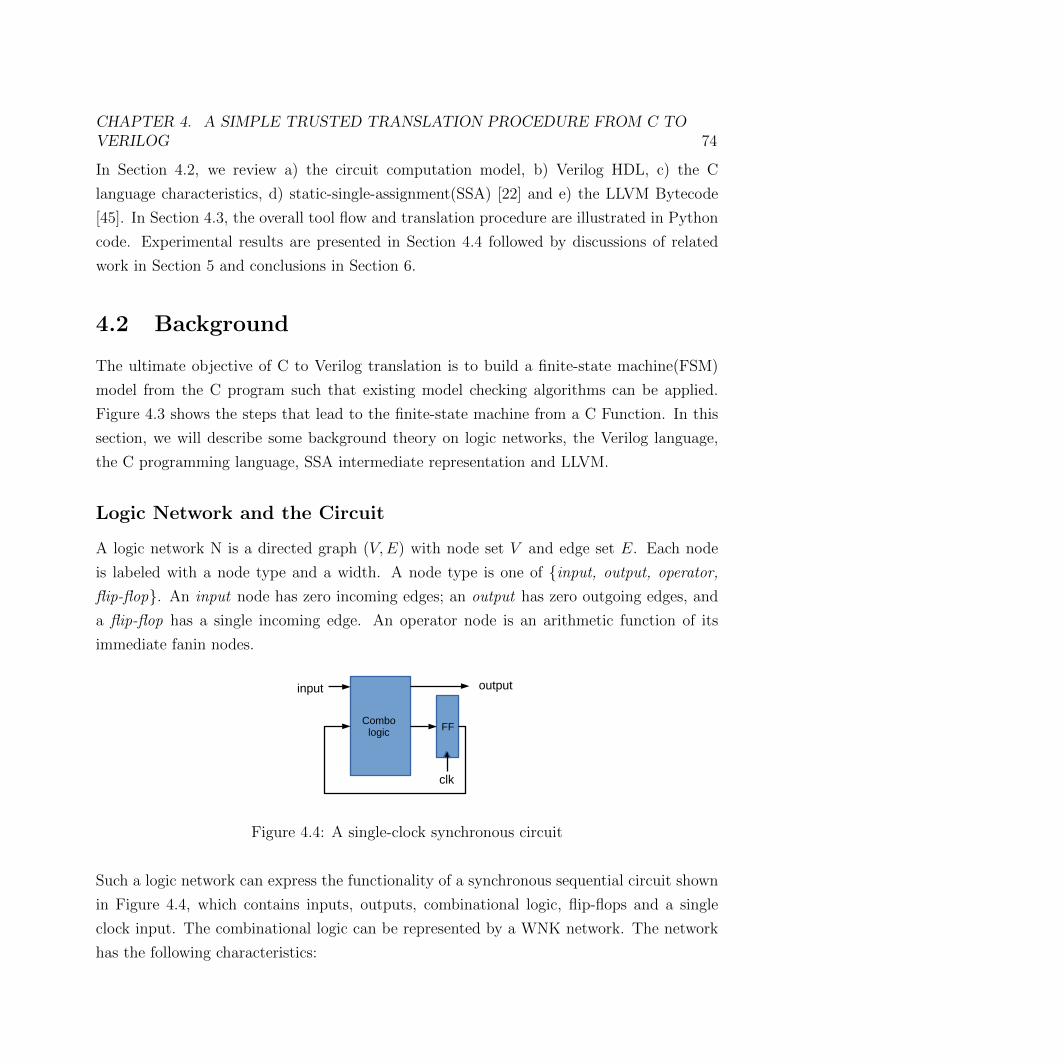
CHAPTER 4. A SIMPLE TRUSTED TRANSLATION PROCEDURE FROM C TOVERILOG 74
In Section 4.2, we review a) the circuit computation model, b) Verilog HDL, c) the C
language characteristics, d) static-single-assignment(SSA) [22] and e) the LLVM Bytecode
[45]. In Section 4.3, the overall tool flow and translation procedure are illustrated in Python
code. Experimental results are presented in Section 4.4 followed by discussions of related
work in Section 5 and conclusions in Section 6.
4.2 Background
The ultimate objective of C to Verilog translation is to build a finite-state machine(FSM)
model from the C program such that existing model checking algorithms can be applied.
Figure 4.3 shows the steps that lead to the finite-state machine from a C Function. In this
section, we will describe some background theory on logic networks, the Verilog language,
the C programming language, SSA intermediate representation and LLVM.
Logic Network and the Circuit
A logic network N is a directed graph (V,E) with node set V and edge set E. Each node
is labeled with a node type and a width. A node type is one of {input, output, operator,
flip-flop}. An input node has zero incoming edges; an output has zero outgoing edges, and
a flip-flop has a single incoming edge. An operator node is an arithmetic function of its
immediate fanin nodes.
Combo logic FF
clk
input output
Figure 4.4: A single-clock synchronous circuit
Such a logic network can express the functionality of a synchronous sequential circuit shown
in Figure 4.4, which contains inputs, outputs, combinational logic, flip-flops and a single
clock input. The combinational logic can be represented by a WNK network. The network
has the following characteristics:

CHAPTER 4. A SIMPLE TRUSTED TRANSLATION PROCEDURE FROM C TOVERILOG 75
• The logic network topology is statically determined and does not change during eval-
uation of the network.
• The circuit evaluates at every clock cycle and infinitely over time.
The goal is to map a C program into a logic network such that an evaluation of it produces
the same input/output behavior as the original C program.
Verilog HDL
Verilog is an almost de facto standard used by industry for specifying hardware designs. Table
4.2 summarizes its language constructs. The always ff block is used to describe sequential
logic where flip-flops are inferred, while always comb is for combinational logic. According to
Verilog’s event-driven semantics, for the circuit in Figure 4.4, the always blocks are evaluated
every clock cycle, and the computation is infinite over time.
Language elements Verilog Constructsvariables wire /reg
control flow if/else/casesequential block always ff @(posedge clk)
combo block always comboperators +,−, ∗, /,&, |, etc.
Table 4.2: Verilog language elements
Figure 4.5 is a Verilog module for factorial computation. In addition to the integer n as
the input and output ret for the factorial function ret = factorial(n), the module also has
an input start and output ready signals: start and ready are used to indicate the starting
time and ending time of the computation. The waveform in Figure 4.6 illustrates the Verilog
computation of factorial(6) by plotting the value of signals at every cycle. The computation
starts at cycle 0 and ends at cycle 6, between the rising edge of start and ready. Signal values
that are not relevant during the computation are grayed out in the waveform. The goal in
our translation procedure from C to Verilog is to build a Verilog module that implements the
C function such that the computation of the original C function can be obtained between
the rising edges of start and ready.

CHAPTER 4. A SIMPLE TRUSTED TRANSLATION PROCEDURE FROM C TOVERILOG 76
module verilog_factorial
( input clock,
input [31:0] n,
input START,
output reg READY,
output reg [31:0] ret
) ;
reg [31:0] n_reg;
reg [31:0] i_reg;
reg [31:0] ret_cur;
reg [31:0] i_cur;
reg READY_cur;
always_comb begin
ret_cur = ret_reg * i_reg;
i_cur= i_reg + 1;
READY_cur= i_reg==n_reg;
end
always_ff @(posedge clock)
if(START) begin
n_reg<=N;
i_reg<=1;
READY<=0;
ret_reg <= 1;
end else if (i<=n_reg) begin
ret <= ret_cur;
i <= i_cur;
READY <= READY_cur;
end
endmodule
Figure 4.5: Verilog factorial implementation
The C Programming Language
The C language has two major features. One is the control flow structure that defines the
order of computation; the other is the resource allocation, which can be dynamic at run-time.
Conceptually, resources refer to those computation elements that either hold the value of a
variable, or implement some arithmetic function. Static resources are allocated at compile
time, while dynamic resources can be acquired and released during run-time. Table 4.3 lists
the major C features and their category, static or dynamic.
Language Elements C Constructs Resourcevariable local/global static
control flow if/case/for/while staticmemory malloc/free dynamic
parallelism pthread dynamiccall stack function calls dynamicpointers pointer arithmetic aliasing
Table 4.3: C language elements
Pointers are simply aliases for objects in the C program. Although they can be complex to

CHAPTER 4. A SIMPLE TRUSTED TRANSLATION PROCEDURE FROM C TOVERILOG 77
Figure 4.6: Waveform for Module verilog factorialwithn = 6
reason about, there is no resource allocation involved in their use, and thus not a funda-
mental barrier in translating to a circuit model. On the other hand, run-time function calls
can dynamically allocate resources for the stack space to hold local variables. Nested non-
recursive function calls can be eliminated at compile time by function inlining. Dynamic
threads also require run-time acquisition of local variable space and operator nodes. Al-
though the behavior of loops can vary at run time, the computational resources for variable
space can be statically determined during compilation. Therefore if the resources required
for a C program to execute can be statically determined, then the C program execution is
mathematically a finite-state-machine model which can be constructed through Verilog as a
logic network.
Static Single Assignment (SSA)
Static single assignment (SSA) [22] is a break-through concept and technique in compiler
theory and implementation. It is used as an intermediate representation (IR) by translating

CHAPTER 4. A SIMPLE TRUSTED TRANSLATION PROCEDURE FROM C TOVERILOG 78
a program into a sequence of basic blocks with only assignment statements, branching state-
ments and function calls, and most importantly, each variable in SSA is assigned exactly
once. Our translation procedure is based on this principle of the SSA IR. To illustrate the
basic ideas behind static single assignment, we use an example in Figure 4.7 to show how
SSA IR is obtained through a normalization step where the C program’s loop constructs are
rewritten into if-else and goto statements.
int
factorial(int n )
{
int ret = 1;
int i;
for(i=1;i<=n;i++)
{
ret = ret*i;
}
return ret;
}
(a) C function
int
factorial (int n) {
entry:
ret = 1;
i = 1;
goto for_cond;
for_cond:
cond = i<=n;
if (cond)
goto for_body;
else
goto for_end;
for_body:
ret = ret*i;
goto for_inc
for_inc:
i = i+1;
goto for_cond;
for_end:
return ret;
}
(b) Normalized C
entry:
ret0 = 1
i0 = 1
br for_cond
for_cond:
ret1=phi(ret0, ret2)
i1 =phi(i0, i2)
cond i1<=n
br cond for_body for_end
for_body:
ret2 = ret1*i1;
br for_inc
for_inc:
i2 = i1+1
br for_cond
for_end:
return ret1
(c) SSA IR
Figure 4.7: C to SSA IR illustration
In Figure 4.7b, the for loop construct in the factorial function in Figure 4.7a is rewritten
using if-else and goto statements, with four blocks labeled as for cond, for body, for inc and
for end. Following the C language semantics, this transformation is a syntactical rewrite and
can rewrite arbitrary nested loops. It normalizes any C program into a sequence of basic
blocks with the following characteristics:
1. The resulting C program uses only assignment statements, if-else, goto statements

CHAPTER 4. A SIMPLE TRUSTED TRANSLATION PROCEDURE FROM C TOVERILOG 79
(function calls are not considered as they can be eliminated through an inlining pro-
cedure during preprocessing).
2. After normalization, the program is partitioned into a sequence of basic blocks: a label
is defined at the beginning of each block; each block starts with a sequence of assign-
ment statements; the last statement of the block is either a goto or a return statement.
The if-else construct can only be used with the goto statement for conditional branch-
ing. There is a unique basic block labeled with entry which corresponds to the starting
point of the C program.
Compiler theory states that any C program can be normalized into such a basic block
format. This basic block format in 4.7b is almost a compliant SSA form in 4.7c except
for two differences. First, SSA introduces a br operator as a shorthand for goto statement
and conditional branching: ”br label” is the same as ”goto label” and ”br cond label true
lable false” is the same as
if (cond)
goto label_true;
else
goto label_false;
The other difference between the program in Figure 4.7b and the SSA form in Figure 4.7c is
that variables in 4.7b can be assigned in multiple locations (SSA requires each variable be
assigned only once), e.g. ret is assigned in both entry and for body blocks. The rule of the
SSA form is that each variable is assigned only once in the entire program. To achieve this,
at each assignment statement, the left-hand variable is assigned a unique variable id. For
example, in Figure 4.7c, ret0 and ret2 are used for the assignment to ret in the entry and
for body blocks.
However, this leads to the problem that ret1 referenced in the right-hand side of
ret2 = ret1*n
needs be resolved to either ret0 or ret2 because variable ret is assigned at two different
locations. SSA introduces a new operator phi(v0, v1, ..., vi, ...) which returns the resolved

CHAPTER 4. A SIMPLE TRUSTED TRANSLATION PROCEDURE FROM C TOVERILOG 80
value. When the phi(v0, v1, ..., vi, ...) operator is executed, it evaluates to one of the vi based
on the execution history: i.e. the sequence of basic blocks it has visited before entering the
current basic block. In the factorial example,
for_cond:
ret1 = phi(ret0,ret2)
ret1 is resolved to ret0 if the previous basic block’s label is entry, otherwise ret1 is resolved
to ret2 if the previous block’s label is for inc.
CFG for 'factorial' function
entry: br label %for.cond
for.cond: %ret.0 = phi i32 [ 1, %entry ], [ %mul, %for.inc ] %i.0 = phi i32 [ 1, %entry ], [ %inc, %for.inc ] %cmp = icmp sle i32 %i.0, %n br i1 %cmp, label %for.body, label %for.end
T F
for.body: %mul = mul nsw i32 %ret.0, %n br label %for.inc
for.end: ret i32 %ret.0
for.inc: %inc = add nsw i32 %i.0, 1 br label %for.cond
Figure 4.8: LLVM CFG
The introduction and resolution of the phi operator is one of the original contributions of
the SSA form [22]; readers should refer to [22] for a complete and rigorous presentation of

CHAPTER 4. A SIMPLE TRUSTED TRANSLATION PROCEDURE FROM C TOVERILOG 81
the SSA form. Once the SSA form is obtained from the C compilation, the translation of
SSA into Verilog is relatively simple.
LLVM Bytecode
The reason we chose the LLVM compiler infrastructure in this project is that the LLVM
tool chain translates C programs into LLVM Bytecode which is an SSA implementation.
Figure 4.8 is the actual translated LLVM Bytecode of the factorial function in Figure 4.7a
illustrated as a control flow graph(CFG). Each node in the CFG is a labeled basic block,
while the edges in the CFG are derived from the branching operator br. We leave the reader
to refer to the LLVM reference manual [45] for further details on the definition of LLVM
syntax and internal implementations.
4.3 Translating SSA to Verilog
We will describe our translation procedure in terms of SSA terminology because the specifics
of LLVM Bytecode is not as important as the fact that the correctness of our algorithm is
based on the principles of SSA.
From SSA to SSAb: Reverting the phi operator
The first step in the translation process is to revert the phi operator in the SSA intermediate
representation. For each vphi = phi(v0, v1, ..., ) statement, we do the following:
1. Immediately after the location where vi is assigned, add the following assign statement
vphi = vi
2. Remove this vphi = phi(v0, v1, ..., ) statement from the SSA representation
Figure 4.9 shows the reverted SSA representation after the phi statement in Figure 4.7c is
reverted to actual assignments. We call this the SSAb form because after the reverting step,
it no longer satisfies the SSA rule that each variable is assigned only once. However, SSAb
still has the following two characteristics:

CHAPTER 4. A SIMPLE TRUSTED TRANSLATION PROCEDURE FROM C TOVERILOG 82
1. It is in normalized C form. This ensures that each C operator in the SSA IR has a
corresponding Verilog operator for translation.
2. Within each basic block, each SSA variable is assigned only once. This is important
as it simplifies the algorithm when mapping a C variable to the corresponding Verilog
signal during translation.
As described in the next section, translation to Verilog is conducted over the basic blocks
one-by-one; there is no need to require that each variable is globally assigned once. The
above two properties that the SSAb IR satisfies, allows a simple translation procedure from
C to Verilog.
entry:
ret0 = 1
ret1 = ret0 // added from tmp=phi(ret0,ret2)
i0 = 1
i1 = i0 // added from i1=phi(i0,i2)
br for_cond
for_cond:
//removed: ret1=phi(ret0, ret2)
//removed: i1 =phi(i0, i2)
cond i1<=n
br cond for_body for_end
for_body:
ret2 = ret1*i1
ret1 = ret2 // added from tmp=phi(ret0, ret2)
br for_inc
for_inc:
i2 = i1+1
i1 = i2 // added from i1=phi(i0,i2)
br for_cond
for_end:
return ret1
Figure 4.9: SSAb from SSA in Figure 4.7c with phi node reverted
Verbatim Translation to Verilog
The goal of the translation procedure is to create a Verilog module that can be synthesized
to the logic network in Figure 4.10 where the execution of the C program is mapped to
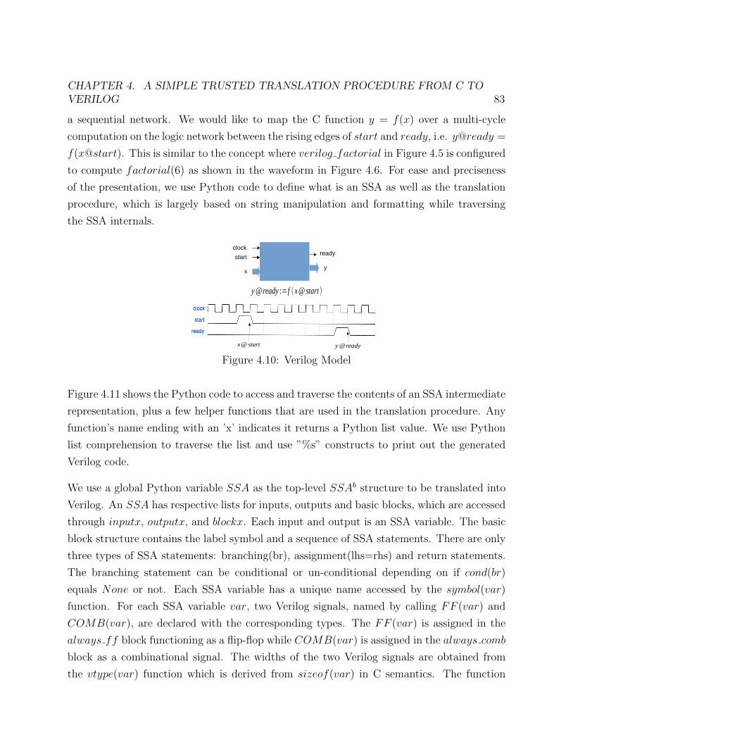
CHAPTER 4. A SIMPLE TRUSTED TRANSLATION PROCEDURE FROM C TOVERILOG 83
a sequential network. We would like to map the C function y = f(x) over a multi-cycle
computation on the logic network between the rising edges of start and ready, i.e. y@ready =
f(x@start). This is similar to the concept where verilog factorial in Figure 4.5 is configured
to compute factorial(6) as shown in the waveform in Figure 4.6. For ease and preciseness
of the presentation, we use Python code to define what is an SSA as well as the translation
procedure, which is largely based on string manipulation and formatting while traversing
the SSA internals.
start
clock
xy
ready
y@ready :=f (x@ start )
Figure 4.10: Verilog Model
Figure 4.11 shows the Python code to access and traverse the contents of an SSA intermediate
representation, plus a few helper functions that are used in the translation procedure. Any
function’s name ending with an ’x’ indicates it returns a Python list value. We use Python
list comprehension to traverse the list and use ”%s” constructs to print out the generated
Verilog code.
We use a global Python variable SSA as the top-level SSAb structure to be translated into
Verilog. An SSA has respective lists for inputs, outputs and basic blocks, which are accessed
through inputx, outputx, and blockx. Each input and output is an SSA variable. The basic
block structure contains the label symbol and a sequence of SSA statements. There are only
three types of SSA statements: branching(br), assignment(lhs=rhs) and return statements.
The branching statement can be conditional or un-conditional depending on if cond(br)
equals None or not. Each SSA variable has a unique name accessed by the symbol(var)
function. For each SSA variable var, two Verilog signals, named by calling FF (var) and
COMB(var), are declared with the corresponding types. The FF (var) is assigned in the
always ff block functioning as a flip-flop while COMB(var) is assigned in the always comb
block as a combinational signal. The widths of the two Verilog signals are obtained from
the vtype(var) function which is derived from sizeof(var) in C semantics. The function

CHAPTER 4. A SIMPLE TRUSTED TRANSLATION PROCEDURE FROM C TOVERILOG 84
DEFx(var) returns a list of the SSA assignments where var is assigned on the left-hand
side (i.e. where lhs(stmt) equals var). By definition of the SSA form, the length of the
returned list from DEFx(var) should always be one, except for those variables (call them
phi variables) that are obtained from reverting the phi statement in the rewriting step.
Figure 4.12 shows the complete implementation of the translation procedure to Verilog given
the above SSA traversal and access functions. The code for gen rhs and gen from stmt are
described and defined in Figure 4.13. For demonstration, Figure 4.14 shows the resulting
Verilog module translated from the SSA structure in Figure 4.9.
The strategy of the translation is to build a logic network such that at each cycle exactly one
basic block is executed. For each basic block’s label in the SSA, we define a LABEL signal
in the Verilog module functioning as a flip-flop: it is assigned to zero or one depending on
whether the corresponding basic block is to be executed in the next cycle. In the generated
Verilog, it has one always ff block and one always comb block. The always comb basically
translates all SSA assignment statements into corresponding Verilog blocking assignments
by following the order within each basic block. The ordering between basic blocks can be
arbitrary.
Function gen from basic block(b) shows each basic block is converted to an if(cond) block
in the always ff block and the conditional expression cond is signal LABEL(b). Signal
LABEL(b) is cleared to zero in the very first statement entering the if block. In the function
gen from br(br, block) in Figure 4.13, the corresponding LABEL signal is set to one for the
next basic block to be entered. In addition, function gen START block(SSA) is used to
trigger the starting point of the execution by setting LABEL entry to one if START is one.
In the Verilog module, when translating the SSA variable var to the corresponding Verilog
signal, we need to choose between COMB(var) and FF (var). The resolution algorithm
is implemented using function PHI(var, stmt, b) in Figure 4.12, where var is referenced
in stmt in block b. This function returns COMB(var) if the var has only one location
where it is assigned (i.e. len(DEFx(var)) == 1), and that location is before the stmt (i.e.
DEFx(var)[0] < stmt) and within the current block b (i.e. DEFx(var)[0] in stmtx(b)).
The PHY function returns FF (var) if otherwise. If the var has more than one location
where it is assigned, then they must not be in the block b, because they were created from
SSA to SSAb for the phi operators when they were reverted to assignment statements in a
different basic block. Hence, these var references would be resolved to the FF (var) signals.

CHAPTER 4. A SIMPLE TRUSTED TRANSLATION PROCEDURE FROM C TOVERILOG 85
For the return statement, the READY signal is assigned 1 and because the rest of the
LABEL signals are cleared to 0, then the execution terminates there after.
Our actual implementation is based on LLVM Bytecode. After the LLVM Bytecode is
obtained from LLVM compilation of the C progream, the C-to-Verilog procedure mainly in-
volves list traversal, string manipulation, and formatting to write out the Verilog code. There
is no cone-of-influence analysis, such that the procedure basically traverses the SSA twice to
generate one always comb and one always ff block. Figure 4.15 shows the waveform that
c2v factorial is evaluated to between START and READY , calculating the ret@READY
to be 720 given the input n@START = 6.
In summary, the C-to-Verilog translation procedure build a logic network that can be used to
model the execution semantics of the original C program. Using the LLVM compiler infras-
tructure to compile the C program into LLVM Bytecode, the translation procedure is built
by traversing the LLVM Bytecode which is an SSA intermediate representation. To build the
logic network from the SSA representation, we use Verilog as the intermediate language to
declare LABEL, FF and COMB signals. The control flow of the SSA is implemented using
the LABEL signals by mapping the basic block into an if block in the always ff block.
Variable reference resolution is implemented using the PHI(var, stmt, block) function, re-
solving the signal value to either the FF or the COMB signal. In doing so, although the
final logic network can be redundant and not optimized at all, the translation procedure is
so simple it basically traverses the SSA basic blocks one by one and conducts an almost ver-
batim translation. In the next section, experimental results show promising and competitive
results in applying this translation procedure to sequential equivalence checking between C
and Verilog as well as in the software verification domain.
Assertions
In the above framework, a C assertion assert(a) is translated into SystemVerilog Assertions
(SVA) [1] with the following form:
assert property (@(posedge clk) label_t|-> v_a );
where label t is the condition in entering the basic block of assert(a) and v a is the corre-
sponding value of a at the time of executing the assert(a) statement in this basic block. The

CHAPTER 4. A SIMPLE TRUSTED TRANSLATION PROCEDURE FROM C TOVERILOG 86
global SSA
##
## SSA construct
##
def inputx(ssa):
# return input variables
def outputx(ssa):
# return output variables
def blockx(ssa):
# return basic blocks
def ssaAssignStmtx(ssa):
# return all assignment
# statements
##
## SSA variable
##
def symbol(var):
#return :
# the name of var as a string
def width(var):
#return sizeof(var) in C
def vtype(var):
return "" if width(var)==1
else '[%d:0]'% (width(var)-1)
def COMB(var):
return "%s_COMB" % symbol(var)
def FF(var):
return "%s_FF" % symbol(var)
def DEFx(var):
return [i for i in
ssaAssignStmtx(SSA)
if lhs(i) == var]
##
## SSA Basic block
##
def label(b):
# return :
# label of the basic block
def LABEL(b):
return "LABEL_%s" % label(b)
def stmtx(b)
# return :
# the list of the statements
# in basic block b
def assignStmtx(b):
# return :
# the list of assign statements
# i.e. lhs=rhs
##
## Br Statement:
## br <label>
## br <cond> <l_true> <l_false>
##
def label(br):
return <label>
def cond(br):
return <cond>
def label_true(br):
return <l_true>
def label_false(br):
return <l_false>
##
## Assignment Statement: lhs=rhs
##
def lhs(assign_stmt):
#return the lhs variable
def rhs(assign_stmt):
#return the rhs expression
##
## Return Statement:
## return val
##
def retval(ret_stmt):
#return val
##
## The PHI func
##
def PHI(var, stmt, b):
assert stmt in stmtx(b)
assert var is rhs(stmt)
if len(DEFx(var))==1 and
DEFx(var)[0] in stmtx(b) and
DEFx(var)[0] < stmt :
return COMB(var)
else:
return FF(var)
Figure 4.11: SSA access and utility functions

CHAPTER 4. A SIMPLE TRUSTED TRANSLATION PROCEDURE FROM C TOVERILOG 87
def C_to_verilog_translate(SSA):
# step 1.1
print """
module c2v_%s(
input clock,
input START,
output READY,
""" %(symbol(SSA))
# step 1.2
delcare_input_ports(SSA)
# step 1.3
declare_output_ports(SSA)
print ');'
# step 2.1
declare_input_signals(SSA)
# step 2.2
declare_label_signals(SSA)
#step 2.3
delclare_lhs_signals(SSA)
#step 3
print 'always_comb begin'
gen_always_comb(SSA)
print 'end // always_comb'
#step 4
print 'always_ff @(posedge clock)'
print 'begin'
#step 4.1
gen_START_block(SSA)
print ' else begin'
#step 4.2
for b in blocks(SSA):
gen_from_basic_block(b)
print ' end'
print 'end // always_ff'
print 'endmodule'
return
def declare_input_ports(SSA):
for i in inputx(SSA):
print 'input %s %s;'
% (vtype(i), symbol(i))
def declare_output_ports(SSA):
for i in outputx(SSA):
print 'output reg %s %;'
% (vtype(i), symbol(i))
def declare_input_signals(SSA):
for i in inputx(SSA):
print 'reg %s %s %s;'
%(vtype(i), FF(i), COMB(i))
def declare_label_signals(SSA):
for i in blockx(SSA):
print 'reg %s;'%(LABEL(i))
def declare_lhs_signals(SSA):
for i in assignStmtx(SSA):
v = lhs(i)
print 'reg %s %s, %s;'
% (vtype(v), FF(v), COMB(v))
def gen_always_comb(SSA):
for b in blockx(SSA):
for i in assignStmtx(b):
print '%s = %s;'
% (COMB(lhs(i)),
gen_rhs(i,b))
def gen_START_block(SSA):
print 'if (START) begin'
for i in inputx(SSA):
print '%s<=%s;'% (FF(i),symbol(i))
print 'LABEL_entry<=1;'
for i in blockx(SSA):
if label(i)!='entry':
print '%s<=0;' %LABEL(i)
print 'end'
def gen_from_basic_block(b):
print '''if(%s) begin
%s<=0;
''' % (LABEL(b), LABEL(b))
for i in stmtx(b):
gen_from_stmt(i,b)
Figure 4.12: SSAb to Verilog Translation

CHAPTER 4. A SIMPLE TRUSTED TRANSLATION PROCEDURE FROM C TOVERILOG 88
def gen_from_stmt(stmt,block):
# based on type of stmt
# call one of
# gen_from_br
# gen_from_return
# gen_from_assign
def gen_from_br(br,block):
if(cond(br)): # conditional
print '''
if(%s) %s <= 1;
else %s <= 0;
'''
%(PHI(cond(br)),br,block),
LABEL(label_true(br)),
LABEL(label_false(br))
else: # unconditional
print '%s<=1;'
% LABEL(label(br))
def gen_from_return(ret,block):
print "ret <= %s;"
%(PHI(retval(ret),ret,block))
print 'READY<=1;'
def gen_from_assign(assign, block):
print '%s<=%s;'
%(FF(lhs(a)), gen_rhs(a))
def gen_rhs(assign,block):
# write out the Verilog equivalent
# expression for rhs(assign)
# 1.map the operator to the
# Verilog equivalent
# 2.replace each operand opnd
# in the rhs expression with
# PHI(opnd,assign,block)
Figure 4.13: Translation to Verilog continued
semantics of the assertion, checks that if label t is true then v a must be true in the same
cycle.
Similarly, a termination conditional check of the C program becomes a liveness check on the
Verilog module in the following SVA assertion:
assert property (@(posedge clk)
start|-> eventually ready);
where start and ready are the signals in the translated Verilog model illustrated in Figure
4.10. The start |−> eventually ready expression means that if start is true, then ready
will be true eventually (sometime in the future).
Memory errors in C that result in signal SIGSEGV will cause the C program to stop. In
the Verilog model, such an error will result in an undefined state in the circuit. Extra logic

CHAPTER 4. A SIMPLE TRUSTED TRANSLATION PROCEDURE FROM C TOVERILOG 89
module c2v_factorial(
//step 1.1
input clock,
input START,
output reg READY,
//step 1.2
input [31:0] n,
//step 1.3
output reg [31:0] ret) ;
// step 2.1
reg[31:0] n_FF, n_COMB;
// step 2.2
reg LABEL_entry;
reg LABEL_for_cond;
reg LABEL_for_body;
reg LABEL_for_inc;
reg LABEL_for_end;
// step 2.3
reg[31:0] ret0_FF, ret0_COMB;
reg[31:0] i0_FF, i0_COMB;
reg[31:0] ret1_FF, ret1_COMB;
reg[31:0] ret2_FF, ret2_COMB;
reg[31:0] i1_FF, i1_COMB;
reg cond_FF, cond_COMB;
reg[31:0] i2_FF, i2_COMB;
// step 3
always_comb begin
// step 3.1
n_COMB = n;
// step 3.2
ret0_COMB = 1;
ret1_COMB = ret0_COMB;
i0_COMB = 1;
i1_COMB = i0_COMB;
cond_COMB = i1_FF <= n_FF;
ret2_COMB = ret1_FF * i1_FF;
ret1_COMB = ret2_COMB;
i2_COMB = i1_FF+1;
i1_COMB = i2_COMB;
end // always_comb
//step 4
always_ff @(posedge clock) begin
//step 4.1
if(START) begin
READY<=0;
n_FF <=n; // input
LABEL_entry<=1; // label
LABEL_for_cond<=0;
LABEL_for_body<=0;
LABEL_for_inc<=0;
LABEL_for_end<=0;
end else begin
// step 4.2
if (LABEL_entry) begin
LABEL_entry<=0;
ret0_FF<=1;
ret1_FF<= ret0_COMB;
i0_FF<= 1;
i1_FF<= i0_COMB;
LABEL_for_cond <= 1;
end
// step 4.2
if(LABEL_for_cond) begin
LABEL_for_cond<=0;
cond_FF = i1_FF<= n_FF;
if(cond_COMB) LABEL_for_body<=1;
else LABEL_for_end<=1;
end
// step 4.2
if (LABEL_for_body) begin
LABEL_for_body<=0;
ret2_FF<= ret1_FF*i1_FF;
ret1_FF<=ret2_COMB;
LABEL_for_inc <=1;
end
// step 4.2
if (LABEL_for_inc) begin
LABEL_for_inc<=0;
i2_FF<=i1_FF+1;
i1_FF<= i2_COMB;
LABEL_for_cond <=1;
end
// step 4.2
if (LABEL_for_end) begin
LABEL_for_end <=0;
ret <= ret1_FF; // output
READY<= 1;
end
end
end // always_ff
endmodule
Figure 4.14: Translated Verilog module from the SSAb in Figure 4.9

CHAPTER 4. A SIMPLE TRUSTED TRANSLATION PROCEDURE FROM C TOVERILOG 90
Figure 4.15: Waveform for Verilog module factorial
or assertions can be added to detect such an error condition when it happens. For memory
error-free C programs, the above translation captures the exact semantics of the C program.
4.4 Experiments
The following experiments were conducted on a 32-core Intel Xeon 2.6GHz machine running
Ubuntu Linux. For equivalence checking between a C program and a Verilog program as
well as model checking a C program for safety properties, the model checker suprove (aka
super prove) from ABC[2] was used with a timeout set to 900 seconds. suprove was the
winner of the last four Hardware Model Checking Competitions (HWMMC - 2012, 2013,
2014 and 2015) in the single-output safety category [29]; suprove is a parallel proof engine
that uses multiple model checking algorithms.
Equivalence Checking - C vs. RTL, FPU Verification
In this experiment, we conducted FPU verification of two OpenCores FPU designs: fpu 100
and fpu double. Both were designed in Verilog and were intended to implement and conform
to the IEEE 754 standard: fpu 100 is a 32-bit and fpu double a 64-bit floating point unit. A
floating point number is represented using 3 components starting from the left of a 32- or 64-
bit-vector (i.e. MSB): a single-bit sign bit, an exponent, and a mantissa. In such a number
system, two special numbers, sNaN and qNaN, are used to represent non-real numbers (not-
a-number) - useful for handling exceptions. For both sNaN and qNaN, the exponent needs be

CHAPTER 4. A SIMPLE TRUSTED TRANSLATION PROCEDURE FROM C TOVERILOG 91
all 1’s and the mantissa to be non-zero. A floating point operation is a function that takes two
floating point numbers as inputs and produces a floating point number as the result, as well
as a set of exception flags: inexact, underflow, overflow, invalid and divide − by − zero.For equivalence checking, the computed floating-point number and exception flags are all
outputs of the logic design to be compared in the miter model. The goal of equivalence
checking is not to tell which model is correct, but to tell if the two models are functionally
equivalent – producing the same results for any legal input values.
Both designs,fpu 100 and fpu double, support add, subtract, multiply, divide, and square-
root operations. Conforming to the IEEE standards, all operators raise exception flags if the
computation underflows, overflows, or produces inexact results. Both designs are configured
to run in the round to nearest even mode and are pipe-lined implementations. They have
the same start-ready model as in Figure 4.10, where an input is driven when start is asserted,
and the result of the FPU operation is available when ready is asserted a number of cycles
later after start.
Two miter models are constructed to compare fpu 100 and fpu double against the C model
from the SoftFloat[30] C library, which is the de facto standard for floating point implemen-
tations. After the C translation to a Verilog model, a miter model is constructed between
the generated Verilog model and the OpenCore model design, comparing the outputs and
the exception flags when both ready signals are asserted. The run-time for each equivalence
checking problem was set to timeout at 900 seconds.
No. Opcode Inputs Softfloat Result RTL Result Pipeline Depth1 add32 matched 62 mul32 000017f0 * 43360000 001104a0 00008825 103 div32 4fdbc9bf / ff800000 80000000 ff800000 334 sqrt32 0000f7c0 1e321421 1dfbd75a 33
Table 4.4: fpu 100 : 32-bit FPU
The Verilog models for opcodes add32 and mul32 are combinational, while div32 and sqrt32
are sequential. Table 4.4 shows the results of comparing the translated SoftFloat program
versus the Verilog fpu 100. It turns out that only for opcode add32 does fpu 100 match with
SoftFloat, while the three other opcodes all have mismatches as shown in the table.
These equivalence checking problems were done under the constraint that no exception flag

CHAPTER 4. A SIMPLE TRUSTED TRANSLATION PROCEDURE FROM C TOVERILOG 92
is generated in the Verilog models, because in the IEEE standard, when an exception is
raised, the result is not defined in certain situations. The input numbers and corresponding
mismatching output results are captured in Table 4.4. Column six is the pipeline depth for
the corresponding operation in the fpu 100 implementation.
No. Opcode InputsSoftfloatResult
RTLResult
PipelineDepth
1 add64 fff8000000000000 + 7ff8000000000000 7ff8000000000000 fff8000000000000 202 add64 d172dd2000000000 + 4175c97000000000 inexact no exception 203 sub64 fdf88d1ffffe7ba4 - fff88d20001e45dc fff88d20001e45dc 7ff88d20001e45dc 214 sub64 d130600000400000 - b131a0020000a41f inexact no exception 215 mul64 8000006e00008194 * 8000001e9e8d5048 inexact , underflow no exception 24
Table 4.5: fpu double: 64-bit FPU
We also compared the Verilog fpu double with SoftFloat’s 64-bit FPU routines. In addition
to comparing the results of each operation, we also conducted equivalence checking of the
exception generation logic. Table 4.5 shows the experiments for opcodes add, subtract and
multiply. All three models generated from the C functions are combinational. Column 2 in
Table 4.5 is the opcode. Column 3 is the inputs to the floating point operation and Column
4 and Column 5 show the difference between the two models under comparison: Tests 1
and 3 produce different output values, while Tests 2, 4, and 5 differ in generating exceptions
flags.
Both fpu double and fpu 100 were completed several years ago and reportedly have been
incorporated into silicon and FPGAs. From the OpenCores repository, each benchmark
includes a random test framework which compares it to SoftFloat for validation. Each have
passed millions of random test vectors. However, from the counterexamples, we observe
that the input numbers that cause the mismatches either contain 10+ consecutive 0s or 1s
(e.g. fff8000000000000 + 7ff8000000000000 ), or the values of both numbers are close to
each other in term Hamming distance (e.g d172dd2000000000 + 4175c97000000000). These
situations are very unlikely to be generated by a random number generator and thus a
random test bench would most likely miss those unusual scenarios. On the other hand
once a miter model is constructed to compare the two designs, sequential/combinational
equivalence checking is much more effective in exposing discrepancies using model-checking
methods. As far as we know, this is the first time these bugs have been reported for this set
of OpenCores designs.

CHAPTER 4. A SIMPLE TRUSTED TRANSLATION PROCEDURE FROM C TOVERILOG 93
Software Verification of Safety Properties
We conducted C verification on the bit-vector benchmarks of the 2015 Software Verification
Competition[7].
Although all participants had bugs, we chose to compare against CPAChecker because it is
an unbounded solver while the other two winners are bounded model checkers. Therefore,
we thought its results are more comparable, although it does produce an incorrect TRUE
result on the function in Figure 4.16.
int main(void) {
unsigned int x = 10;
while (x >= 10) {
x += 2;
}
__VERIFIER_assert(x % 2);
}
Figure 4.16: test:bitvector-loops/overflow false-unreach-call1.i
In the C program under verification, the dummy function VERIFIER nondet int, used to
indicate a random number generator, was converted into a new free primary inputs in the
Verilog modules. The calls to the error flagging function, VERIFIER error, was converted
into SVA assertions. Our program, VeriABC[48], which interfaces with Verific[64] was then
used to compile the generated Verilog and SVA into an AIG[10]. suprove from ABC [2] was
used to prove or dis-prove the target properties.
Figure 4.17 shows the results. CPAChecker’s results were obtained from the official compe-
tition website, which were run on a 3.4Ghz Intel Quad-core i7 platform, while ours were run
on an 32-core Intel Xeon 2.6Ghz host. The second and third columns show ABC’s suprove
results, while the forth and fifth columns are the published results from the competition’s
website. Of the 46 tests, ABC resolved 30 while CPAchecker resolved 40. There are 4 tests
that ABC resolved but CPAChecker did not. The capital letters, TRUE and FALSE, are
indicating the test is solved by only one of the two solvers being compared. The results seem
rather promising for our approach in that suprove is only optimized to run on hardware
model checking problems that have been bit-blasted. Thus no software related heuristics nor
word-level information could be utilized by suprove.

CHAPTER 4. A SIMPLE TRUSTED TRANSLATION PROCEDURE FROM C TOVERILOG 94
So far, we believe our proof results are more trust-worthy because the C-compilation proce-
dure is simple and less error-prone and no inconsistency of the results have been found yet
for suprove.
Test suprove Time CPA Timebyte add 1 true-unreach-call timeout 900 TRUE 34.56byte add 2 true-unreach-call timeout 900 TRUE 78.33byte add false-unreach-call false 7.70 false 63.58diamond false-unreach-call2 false 0.48 false 1.78gcd 1 true-unreach-call true 2.14 true 2.29gcd 2 true-unreach-call true 13.82 true 2.31gcd 3 true-unreach-call true 10.12 true 2.26gcd 4 true-unreach-call true 0.12 true 1.38implicitunsignedconversion false-u false 0.10 false 1.59implicitunsignedconversion true-un true 0.09 true 1.40integerpromotion false-unreach-cal false 0.11 false 2.30integerpromotion true-unreach-call true 0.09 true 1.57interleave bits true-unreach-call true 0.66 true 16.63jain 1 true-unreach-call true 0.10 true 2.52jain 2 true-unreach-call true 0.10 true 2.61jain 4 true-unreach-call true 0.11 true 2.59jain 5 true-unreach-call TRUE 0.10 timeout 930.61jain 6 true-unreach-call true 0.12 true 2.65jain 7 true-unreach-call true 0.12 true 4.97modulus true-unreach-call TRUE 35.57 timeout 903.46num conversion 1 true-unreach-ca true 0.09 true 1.40num conversion 2 true-unreach-ca true 0.90 true 17.07overflow false-unreach-call1 timeout 900 TRUE 122.57parity true-unreach-call timeout 900 timeout 906.63s3 clnt 1 false-unreach-call.BV false 99.51 false 5.75s3 clnt 1 true-unreach-call.BV timeout 900 TRUE 32.85s3 clnt 2 false-unreach-call.BV timeout 900 FALSE 87.28s3 clnt 2 true-unreach-call.BV timeout 900 TRUE 29.56s3 clnt 3 false-unreach-call.BV false 16.77 false 4.48s3 clnt 3 true-unreach-call.BV timeout 900 TRUE 34.83s3 srvr 1 alt true-unreach-call TRUE 518.21 aborted 128.31s3 srvr 1 true-unreach-call.BV timeout 900 TRUE 63.91s3 srvr 2 alt true-unreach-call timeout 900 TRUE 62.97s3 srvr 2 true-unreach-call.BV timeout 900 TRUE 62.91s3 srvr 3 alt true-unreach-call timeout 900 TRUE 63.48s3 srvr 3 true-unreach-call.BV timeout 900 TRUE 63.86signextension2 false-unreach-call false 0.08 false 2.12signextension2 true-unreach-call true 0.09 true 1.54signextension false-unreach-call false 0.12 false 2.18signextension true-unreach-call true 0.09 true 1.56soft float 1 true-unreach-call timeout 900 TRUE 11.35soft float 2 true-unreach-call true 119.53 true 12.70soft float 3 true-unreach-call TRUE 300.46 timeout 930.46soft float 4 true-unreach-call timeout 900 TRUE 63.56soft float 5 true-unreach-call true 138.73 true 13.25sum02 true-unreach-call timeout 900 timeout 903.20
Figure 4.17: Software Verification Benchmark: bitvector category

CHAPTER 4. A SIMPLE TRUSTED TRANSLATION PROCEDURE FROM C TOVERILOG 95
4.5 Related works
Because we are building a finite state machine model directly from a C program, it is more
suitable to compare our work with those software verification flows that do symbolic explo-
ration of the state space using model checking algorithms.
The SLAM model checker [3] introduced Boolean programs – imperative programs where
each variable is Boolean – as an intermediate language to represent program abstractions. A
tool flow was created to convert C programs and predicates to Boolean programs and then
to employ follow-up model checking using abstraction/refinement.
The Blast [9] model checker implements an optimization of CEGAR (Counter Example
Guided Abstraction Refinement) called lazy abstraction. The internal model of the C pro-
gram is built incrementally, based on an error trace and an unrolling of the CFG. A similar
internal representation is used in the IMPACT [49] model checker.
The C verifiers f-soft [33] and CPAChecker [8] internally build a finite state machine model
using their own internal representations. The finite state machine definition is conceptually
the same as the circuit model. Our approach is simpler because Verilog has well defined
syntax and semantics. LLBMC [51] also uses the LLVM infrastructure to translate the C
program only for bounded model checking through loop unrolling.
In the hardware design area, high level synthesis tools Catapult [14] and Forte [27] build
circuits from a subset of the C language. Their primary focus is to optimize the generated
hardware to satisfy user-defined timing, power, and area constraints. In contrast, our goal is
for verification purposes; the translation procedure does not consider memories and does not
restrict the number of flip-flops to use in the Verilog model; optimization is not our concern
at the translation stage because abstraction and optimization can be conducted later on the
Verilog model instead of on the original C program.
The tools AutoPilot [69] and LegUp [16], translate a C program for FPGA synthesis or
hardware and software co-simulation. They use the LLVM framework and translate LLVM
Bytecode into Verilog. There is no detailed description of the underlying translation algo-
rithm. By looking at the generated Verilog from LegUp, their principle seems to be similar
to ours, except they use memory components to allocate memory spaces for each variable
and introduce memory access latency for each read/write of variable values while the control

CHAPTER 4. A SIMPLE TRUSTED TRANSLATION PROCEDURE FROM C TOVERILOG 96
flow graph is instruction based rather than basic block based.
The tool in [19] processes a C program into an SSA-like internal format and conducts bounded
model checking for C to RTL equivalence checking. Our model can be used for both bounded
and unbounded model checking and our implementation is much simpler based on the LLVM
infrastructure.
4.6 Conclusions
In this chapter, we observed that the gap between a C program and a circuit computa-
tional model is due to the use of dynamic resources in the C language: run-time memory
allocation/de-allocation, run-time function call stacks, and parallel threads. We build a sim-
ple translation procedure from a single thread non-recursive C program to a semantically
equivalent Bytecode network using the LLVM compiler. The mapping from LLVM Byte-
code to a Verilog module is then almost verbatim. Experiments show promising and more
consistent results compared to existing software verification approaches.

97
Chapter 5
Conclusion and Possible Future
Extensions
In this thesis, we tackled the two top-level verification tasks of a compilation from the
software language C to an optimized RTL (word-level Verilog description) implementation.
This was broken down into two aspects in reasoning about high-level constructs in software
and hardware verification. The C-to-Verilog procedure of Chapter 4, translates a C-program
into a semantically equivalent but non-optimized Verilog description which preserves the
original high-level control and data structures. The ”verification” here is done by using the
LLVM compiler in a straight-forward manner which relies on the maturity of this compiler
and its extensive use over many years. Thus it is reasonable to rely on the LLVM compiler
producing correct LLVM Bytecode. A step from Bytecode to Verilog was implemented
which relies on the almost verbatim translation of LLVM Bytecode into Verilog. Because of
its simplicity it is reasonable to assume that this step is correct.
The second aspect of the verification is the formal verification step. This intermediate Verilog
output from the C to Verilog step can be compared to another Verilog description which
may be the result of an automatic or manual optimization of this.
The LEC system was created for this step in order to be enhance our ability to verify
difficult equivalence checking of industrial problem created by sophisticated data-path opti-
mizations. LEC is an open system created to reason about and utilize high-level constructs
for data-path equivalence checking. LEC consists of solver widgets, transformation widgets
and learning widgets. Solver widgets are procedures which produces either SAT, UNSAT or

CHAPTER 5. CONCLUSION AND POSSIBLE FUTURE EXTENSIONS 98
UNRESOLVED results of the underlying miter model. The inference rules used in LEC’s
proof are carried out by the transformation widgets while the learning widgets collect struc-
tural and function information of the design so that LEC can heuristically select and decide
how to apply particular transformation widgets. Such an architecture allows a LEC user to
tackle a new miter problem by identifying the bottleneck logic, learn about the design and
to eventually automatically reason at a higher-level to finally establish a composite proof.
In this thesis research we built a practical tool flow to reason about high-level constructs
in C and Verilog programs for formal verification. For future work, LEC could be extended
with new learning widgets to be more powerful in solving data-path equivalence problems as
they arise in practice. Hopefully,because of LEC’s modular structure, these extensions are
made more feasible and easier.
On the software verification front, once a C program is translated into Verilog, existing
hardware verification techniques can be adapted to take advantage of the characteristics of
a software program to improve performance and capacity. A tighter integration of the two
components with GUI and debugging capabilities could transform this thesis work into a
practical industrial strength tool flow for C and RTL data-path formal verification or for
property checking of software programs.

99
Bibliography
[1] 1800: IEEE Standard for System Verilog - Unified Hardware Design, Specification, and
Verification Language. IEEE Computer Society, 2005.
[2] “ABC - A System for Sequential Synthesis and Verification”. In: Berkeley Verification
and Synthesis Research Center, http://www.bvsrc.org.
[3] Thomas Ball and Sriram K Rajamani. “The SLAM project: debugging system software
via static analysis”. In: ACM SIGPLAN Notices. Vol. 37. 1. ACM. 2002, pp. 1–3.
[4] Clark Barrett et al. “Cvc4”. In: Computer Aided Verification. Springer. 2011, pp. 171–
177.
[5] Mohamed Abdul Basith et al. “Algebraic approach to arithmetic design verification”.
In: Formal Methods in Computer-Aided Design (FMCAD), 2011. IEEE. 2011, pp. 67–
71.
[6] Jason Baumgartner et al. “Scalable sequential equivalence checking across arbitrary
design transformations”. In: Computer Design, 2006. ICCD 2006. International Con-
ference on. IEEE. 2007, pp. 259–266.
[7] Dirk Beyer. “Software Verification and Verifiable Witnesses”. In: Tools and Algorithms
for the Construction and Analysis of Systems. Springer, 2015, pp. 401–416.
[8] Dirk Beyer and M Erkan Keremoglu. “CPACHECKER: A tool for configurable software
verification”. In: Computer Aided Verification. Springer. 2011, pp. 184–190.
[9] Dirk Beyer et al. “The software model checker Blast”. In: International Journal on
Software Tools for Technology Transfer 9.5-6 (2007), pp. 505–525.
[10] Armin Biere, Keijo Heljanko, and Siert Wieringa. “AIGER 1.9 and Beyond”. In: Avail-
able at http://fmv.jku.at/hwmcc12/beyond1.pdf (2012).

BIBLIOGRAPHY 100
[11] Per Bjesse and Koen Claessen. “SAT-Based Verification without State Space Traver-
sal”. In: FMCAD ’00: Proceedings of the Third International Conference on Formal
Methods in Computer-Aided Design. London, UK: Springer-Verlag, 2000, pp. 372–389.
isbn: 3-540-41219-0.
[12] Robert Brayton and Alan Mishchenko. “ABC: An academic industrial-strength verifi-
cation tool”. In: Computer Aided Verification. Springer. 2010, pp. 24–40.
[13] Robert Brummayer and Armin Biere. “Boolector: An efficient SMT solver for bit-
vectors and arrays”. In: Tools and Algorithms for the Construction and Analysis of
Systems. Springer, 2009, pp. 174–177.
[14] “Calypto R© Catapult Design Product”. In: http://www.calypto.com.
[15] “Calypto R© SLEC”. In: http://www.calypto.com.
[16] Andrew Canis et al. “LegUp: high-level synthesis for FPGA-based processor/accelerator
systems”. In: Proceedings of the 19th ACM/SIGDA international symposium on Field
programmable gate arrays. ACM. 2011, pp. 33–36.
[17] Michael L Case, Alan Mishchenko, and Robert K Brayton. “Automated extraction of
inductive invariants to aid model checking”. In: Formal Methods in Computer Aided
Design, 2007. FMCAD’07. IEEE. 2007, pp. 165–172.
[18] Alessandro Cimatti et al. “The MathSAT5 SMT Solver”. In: Tools and Algorithms for
the Construction and Analysis of Systems. Springer, 2013, pp. 93–107.
[19] Edmund Clarke, Daniel Kroening, and Karen Yorav. “Behavioral consistency of C and
Verilog programs using bounded model checking”. In: Design Automation Conference,
2003. Proceedings. IEEE. 2003, pp. 368–371.
[20] Robert P Colwell. The Pentium Chronicles: The People, Passion, and Politics Behind
Intel’s Landmark Chips (Software Engineering Best Practices). Wiley-IEEE Computer
Society Pr, 2005.
[21] Jason Cong et al. “High-level synthesis for FPGAs: From prototyping to deployment”.
In: Computer-Aided Design of Integrated Circuits and Systems, IEEE Transactions on
30.4 (2011), pp. 473–491.
[22] Ron Cytron et al. “Efficiently computing static single assignment form and the control
dependence graph”. In: ACM Transactions on Programming Languages and Systems
(TOPLAS) 13.4 (1991), pp. 451–490.
BIBLIOGRAPHY 101
[23] Leonardo De Moura and Nikolaj Bjørner. “Z3: An efficient SMT solver”. In: Tools and
Algorithms for the Construction and Analysis of Systems. Springer, 2008, pp. 337–340.
[24] Bruno Dutertre and Leonardo De Moura. “The yices smt solver”. In: Tool paper at
http://yices. csl. sri. com/tool-paper. pdf 2 (2006), p. 2.
[25] Niklas Een and Niklas Sorensson. “MiniSat-A SAT Solver with Conflict-Clause Mini”.
In: SAT 2005.
[26] Evren Ermis et al. “Ultimate Kojak”. In: Tools and Algorithms for the Construction
and Analysis of Systems. Springer, 2014, pp. 421–423.
[27] “Forte Design Systems”. In: http://www.forteds.com.
[28] Arie Gurfinkel, Temesghen Kahsai, and Jorge A Navas. “SeaHorn: A framework for
verifying C programs (Competition contribution)”. In: Tools and Algorithms for the
Construction and Analysis of Systems. Springer, 2015, pp. 447–450.
[29] Hardware model checking competition 2014. 2014.
[30] John Hauser. “SoftFloat”. In: available from http://www.jhauser.us/arithmetic/SoftFloat.html
(2002).
[31] Matthias Heizmann et al. “Ultimate Automizer with Unsatisfiable Cores”. In: Tools
and Algorithms for the Construction and Analysis of Systems. Springer, 2014, pp. 418–
420.
[32] IEEE standard for binary floating-point arithmetic. Note: Standard 754–1985. New
York: Institute of Electrical and Electronics Engineers, 1985.
[33] F Ivancic et al. “F-Soft: Software verification platform”. In: Computer Aided Verifica-
tion. Springer. 2005, pp. 301–306.
[34] Susmit Jha, Rhishikesh Limaye, and Sanjit A Seshia. “Beaver: Engineering an efficient
smt solver for bit-vector arithmetic”. In: Computer Aided Verification. Springer. 2009,
pp. 668–674.
[35] Ryan Kastner, Anup Hosangadi, and Farzan Fallah. Arithmetic optimization techniques
for hardware and software design. Cambridge University Press, 2010.
[36] Matt Kaufmann, Panagiotis Manolios, and J Strother Moore. Computer-aided reason-
ing: ACL2 case studies. Vol. 4. Springer Science & Business Media, 2013.

BIBLIOGRAPHY 102
[37] Matt Kaufmann, J. Strother Moore, and Panagiotis Manolios. Computer-Aided Rea-
soning: An Approach. Norwell, MA, USA: Kluwer Academic Publishers, 2000. isbn:
0792377443.
[38] Alfred Koelbl et al. “Solver technology for system-level to RTL equivalence checking”.
In: Design, Automation & Test in Europe Conference & Exhibition, 2009. DATE’09.
IEEE. 2009, pp. 196–201.
[39] Daniel Kroening, Edmund Clarke, and Karen Yorav. “Behavioral Consistency of C
and Verilog Programs Using Bounded Model Checking”. In: Proceedings of DAC 2003.
ACM Press, 2003, pp. 368–371. isbn: 1-58113-688-9.
[40] Daniel Kroening and Michael Tautschnig. “CBMC–C bounded model checker”. In:
Tools and Algorithms for the Construction and Analysis of Systems. Springer, 2014,
pp. 389–391.
[41] Andreas Kuehlmann and Jason Baumgartner. “Transformation-based verification us-
ing generalized retiming”. In: Computer Aided Verification. Springer. 2001, pp. 104–
117.
[42] Andreas Kuehlmann and Florian Krohm. “Equivalence Checking Using Cuts and
Heaps”. In: Proceedings of the 34th Annual Design Automation Conference. DAC
’97. Anaheim, California, USA: ACM, 1997, pp. 263–268. isbn: 0-89791-920-3. doi:
10.1145/266021.266090. url: http://doi.acm.org/10.1145/266021.266090.
[43] A. Kuehlmann et al. “Robust Boolean reasoning for equivalence checking and func-
tional property verification”. In: IEEE Transactions on Computer-Aided Design of
Integrated Circuits and Systems, Volume 21, Issue 12. Dec, 2002, pp. 1377–1394.
[44] Chao-Yue Lai, Chung-Yang Huang, and Kei-Yong Khoo. “Improving constant-coefficient
multiplier verification by partial product identification”. In: Design, Automation and
Test in Europe, 2008. DATE’08. IEEE. 2008, pp. 813–818.
[45] Chris Lattner and Vikram Adve. “LLVM: A compilation framework for lifelong pro-
gram analysis & transformation”. In: Code Generation and Optimization, 2004. CGO
2004. International Symposium on. IEEE. 2004, pp. 75–86.
[46] Wenchao Li, Zach Wasson, and Sanjit A. Seshia. “Reverse engineering circuits using
behavioral pattern mining”. In: HOST. 2012, pp. 83–88.

BIBLIOGRAPHY 103
[47] Wenchao Li et al. “WordRev: Finding word-level structures in a sea of bit-level gates”.
In: HOST. 2013, pp. 67–74.
[48] Jiang Long et al. “Enhancing ABC for LTL Stabilization Verification of SystemVer-
ilog/VHDL Models”. In: DIFTS (2011).
[49] Kenneth L McMillan. “Lazy abstraction with interpolants”. In: Computer Aided Ver-
ification. Springer. 2006, pp. 123–136.
[50] Kenneth L McMillan, Andreas Kuehlmann, and Mooly Sagiv. “Generalizing DPLL to
richer logics”. In: Computer Aided Verification. Springer. 2009, pp. 462–476.
[51] Florian Merz, Stephan Falke, and Carsten Sinz. “LLBMC: Bounded model checking
of C and C++ programs using a compiler IR”. In: Verified Software: Theories, Tools,
Experiments. Springer, 2012, pp. 146–161.
[52] A. Mishchenko et al. “Improvements to Combinational Equivalence Checking”. In:
Computer-Aided Design, 2006. ICCAD ’06. IEEE/ACM International Conference on.
2006, pp. 836–843. doi: 10.1109/ICCAD.2006.320087.
[53] Jeremy Morse et al. “ESBMC 1.22”. In: Tools and Algorithms for the Construction
and Analysis of Systems. Springer, 2014, pp. 405–407.
[54] T Nicely. “Bug in the pentium fpu”. In: E-mail to Intel 30 (1994).
[55] V. Paruthi and A. Kuehlmann. “Equivalence checking combining a structural SAT-
solver, BDDs, and simulation”. In: Computer Design, 2000. Proceedings. 2000 Inter-
national Conference on. 2000, pp. 459–464. doi: 10.1109/ICCD.2000.878323.
[56] Evgeny Pavlenko et al. “STABLE: A new QF-BV SMT solver for hard verification
problems combining Boolean reasoning with computer algebra”. In: Design, Automa-
tion & Test in Europe Conference & Exhibition (DATE), 2011. IEEE. 2011, pp. 1–
6.
[57] Namrata Shekhar, Priyank Kalla, and Florian Enescu. “Equivalence verification of
polynomial datapaths using ideal membership testing”. In: Computer-Aided Design of
Integrated Circuits and Systems, IEEE Transactions on 26.7 (2007), pp. 1320–1330.
[58] N. Shekhar et al. “Equivalence verification of polynomial datapaths with fixed-size
bit-vectors using finite ring algebra”. In: Computer-Aided Design, 2005. ICCAD-2005.
IEEE/ACM International Conference on. 2005, pp. 291–296. doi: 10.1109/ICCAD.
2005.1560081.

BIBLIOGRAPHY 104
[59] “smtlib”. In: http://www.smt-lib.org.
[60] W Snyder, P Wasson, and D Galbi. Verilator: Convert Verilog code to C++/SystemC.
2012.
[61] Baruch Sterin et al. “The benefit of concurrency in model checking”. In: IWLS. 2011.
[62] D. Stoffel and W. Kunz. “Equivalence checking of arithmetic circuits on the arith-
metic bit level”. In: Computer-Aided Design of Integrated Circuits and Systems, IEEE
Transactions on 23.5 (2004), pp. 586–597. issn: 0278-0070. doi: 10.1109/TCAD.2004.
826548.
[63] Cesare Tinelli. “A DPLL-based calculus for ground satisfiability modulo theories”. In:
European Workshop on Logics in Artificial Intelligence. Springer. 2002, pp. 308–319.
[64] “Verific Design Automation: http://www.verific.com”. In:
[65] Dexi Wang et al. “Beagle: http://sts.thss.tsinghua.edu.cn/beagle”. In: 2015.
[66] Dong Wang and Jeremy Levitt. “Automatic assume guarantee analysis for assertion-
based formal verification”. In: Proceedings of the 2005 Asia and South Pacific Design
Automation Conference. ACM. 2005, pp. 561–566.
[67] Wei Wang, Clark Barrett, and Thomas Wies. “Cascade 2.0”. In: Verification, Model
Checking, and Abstract Interpretation. Springer. 2014, pp. 142–160.
[68] Markus Wedler et al. “A normalization method for arithmetic data-path verification”.
In: Computer-Aided Design of Integrated Circuits and Systems, IEEE Transactions on
26.11 (2007), pp. 1909–1922.
[69] Zhiru Zhang et al. “AutoPilot: A platform-based ESL synthesis system”. In: High-Level
Synthesis. Springer, 2008, pp. 99–112.
[70] Qi Zhu et al. “SAT sweeping with local observability don’t-cares”. In: Proceedings of
the 43rd annual Design Automation Conference. ACM. 2006, pp. 229–234.