Realistic evaluation of hull performance for rowing shells, canoes,and kayaks in unsteady flow

ALEXANDER DAY1, IAN CAMPBELL2, DAVID CLELLAND1, LAWRENCE J. DOCTORS3,

& JAKUB CICHOWICZ1

1Naval Architecture and Marine Engineering, Strathclyde University, Glasgow, UK, 2Wolfson Unit for Marine Technology

and Industrial Aerodynamics, Southampton University, Southampton, UK and 3School of Mechanical and Manufacturing

Engineering, The University of New South Wales, Sydney, NSW, Australia

(Accepted 28 March 2011)

AbstractIn this study, we investigated the effect of hull dynamics in shallow water on the hydrodynamic performance of rowing shellsas well as canoes and kayaks. An approach was developed to generate data in a towing tank using a test rig capable ofreproducing realistic speed profiles. The impact of unsteady shallow-water effects on wave-making resistance was examinedvia experimental measurements on a benchmark hull. The data generated were used to explore the validity of acomputational approach developed to predict unsteady shallow-water wave resistance. Comparison of measured andpredicted results showed that the computational approach correctly predicted complex unsteady wave-resistance phenomenaat low oscillation frequency and speed, but that total resistance was substantially under-predicted at moderate oscillationfrequency and speed. It was postulated that this discrepancy arose from unsteady viscous effects. This was investigated viahot-film measurements for a full-scale single scull in unsteady flow in both towing-tank and field-trial conditions. Resultssuggested a strong link between acceleration and turbulence and demonstrated that the measured real-world viscous-flowbehaviour could be successfully reproduced in the tank. Thus a suitable tank-test approach could provide a reliable guide tohull performance characterization in unsteady flow.

Keywords: Rowing shell, canoe, kayak, hull performance, hydrodynamics, unsteady flow

Introduction

Background and literature review

In boat-based sports, sailing has long led the way in

the application of physical testing, in test tanks, wind

tunnels and at full-scale, as well as computational

analysis, driven especially by the high budgets of

America’s Cup yacht design. In rowing, canoeing,

and kayaking, the use of both computational hydro-

dynamics and physical testing in performance

assessment has been more limited.

Tuck and Lazauskas (1996) and Lazauskas (1998)

performed steady-speed thin-ship (inviscid) compu-

tational studies of rowing shells. Scragg and Nelson

(1993) used a steady-speed inviscid wave-resistance

code, including shallow-water effects, to predict the

performance and design of two hulls. More recently,

Formaggia and colleagues (Formaggia, Miglio,

Mola, & Montano, 2009; Formaggia, Miglio, Mola,

& Parolini, 2008) computed the effects of heave and

pitch motions on resistance using a potential-flow

approach, and later utilized this in a sophisticated

dynamic model of the rower–hull–fluid system.

Berton and colleagues (Berton, Alessandrini, Barre,

& Kobus, 2007) presented results for an unsteady

viscous computational fluid dynamics (CFD) ap-

proach. Other researchers (e.g. Wellicome, 1967)

have used steady-speed tank tests as an aid to the

development of improved hull forms for rowing

shells; many other tank-test studies carried out

remain commercially confidential.

The application of these techniques to canoes and

kayaks has been more limited. Lazuaskas and Tuck

(1996) applied the steady-speed thin-ship approach

to explore optimal hull forms for racing kayaks;

Lazauskas and Winters (1997) compared the perfor-

mance of optimal hull forms and some real designs.

Bugalski (2009) documents the history of canoe hull-

form development, and outlines a detailed technical

Correspondence: A. Day, Naval Architecture and Marine Engineering, Strathclyde University, 100 Montrose Street, Glasgow G4 0LZ, UK.

E-mail: sandy.day@na-me.ac.uk

Journal of Sports Sciences, July 2011; 29(10): 1059–1069

ISSN 0264-0414 print/ISSN 1466-447X online � 2011 Taylor & Francis

DOI: 10.1080/02640414.2011.576691

Dow

nloa

ded

by [

Uni

vers

ity o

f C

alif

orni

a Sa

nta

Cru

z] a

t 16:

24 1

4 O

ctob

er 2

011

program implemented in support of the design of

Plastex canoes, including tank testing and CFD

applications.

As hull designs evolve, available gains diminish,

and increased demands are placed upon the accuracy

of both experimental and computational approaches.

Nonetheless, the extremely small winning margins

still justify the extraction of every last possible

improvement. In the Beijing Olympics, over the 14

rowing events, 18 crews were within 0.5% of mean

speed of the gold medal-winning crews in their event,

from as low as fourth place, while 33 were within 1%.

Consequently, effects that might have previously

been considered too small or too challenging to

model may need to be considered, even where

inclusion of these effects requires novel approaches.

Two such effects are explored here: the impact of

shallow water, and the effect of unsteady variation in

speed through the stroke.

Effect of water depth

The key parameter in characterizing the effect of

water depth on resistance is the depth Froude Number,

Frh ¼ U=ffiffiffiffiffi

ghp

, where U is boat speed, g is the

gravitational constant, and h is water depth. If

Frh� 0.5, results are similar to deep water. As the

boat approaches the critical speed (Frh¼ 1.0), wave-

lengths, wave heights, and wave resistance all

increase. Indeed, for this reason, high-speed ferries

normally avoid operating in a depth Froude number

range of 0.8–1.2. For supercritical (Frh4 1.0) speeds,

the transverse components of the wave pattern

disappear and the wave resistance may be reduced

compared with the critical value. Faltinsen (2005)

gives a detailed discussion of the effect of water depth

on wave patterns and wave resistance.

On a rowing lake with depth of 3.0 m, the critical

speed is around 5.4 m � s71; many elite rowers will

be travelling at this speed at some point in their

stroke cycle. Hence it is important to be able to

account for the effects of shallow water both

experimentally and computationally in a first-princi-

ples approach to hull design.

Effect of unsteady speed

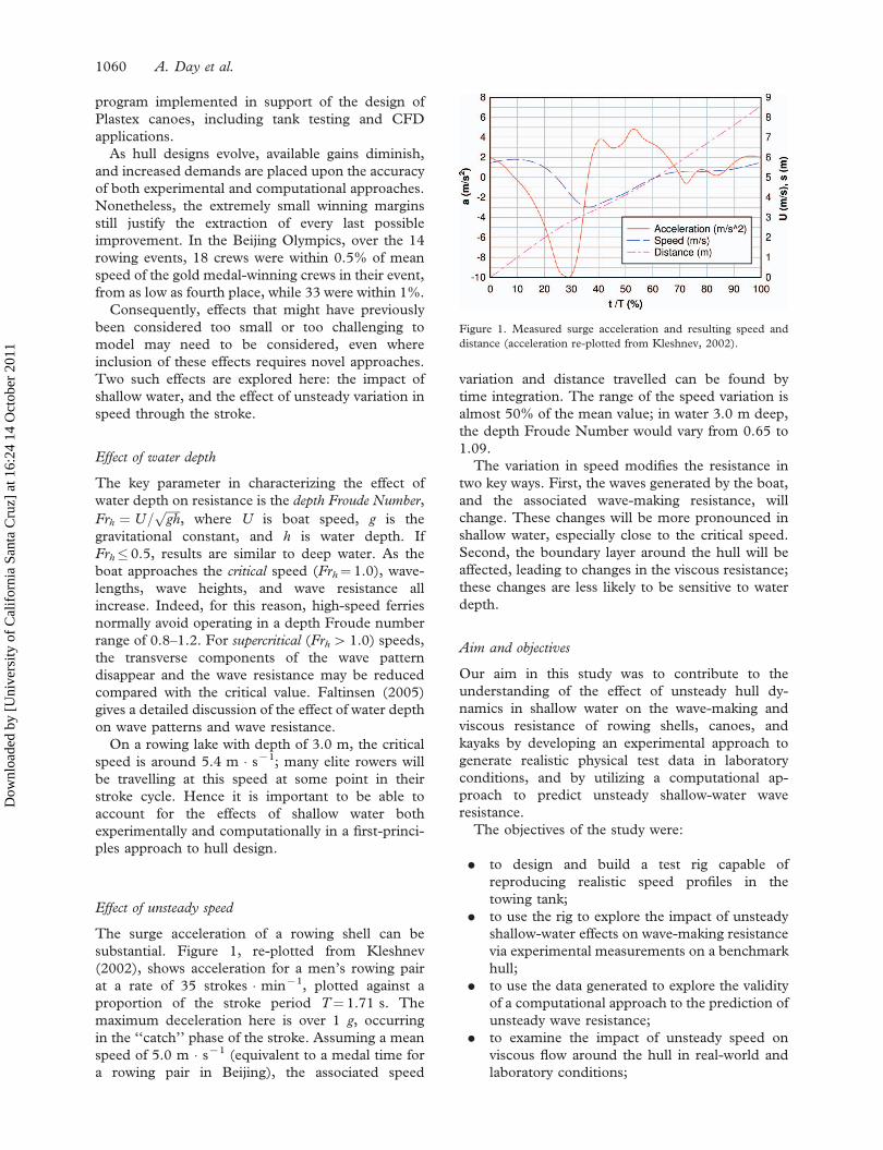
The surge acceleration of a rowing shell can be

substantial. Figure 1, re-plotted from Kleshnev

(2002), shows acceleration for a men’s rowing pair

at a rate of 35 strokes � min71, plotted against a

proportion of the stroke period T¼ 1.71 s. The

maximum deceleration here is over 1 g, occurring

in the ‘‘catch’’ phase of the stroke. Assuming a mean

speed of 5.0 m � s71 (equivalent to a medal time for

a rowing pair in Beijing), the associated speed

variation and distance travelled can be found by

time integration. The range of the speed variation is

almost 50% of the mean value; in water 3.0 m deep,

the depth Froude Number would vary from 0.65 to

1.09.

The variation in speed modifies the resistance in

two key ways. First, the waves generated by the boat,

and the associated wave-making resistance, will

change. These changes will be more pronounced in

shallow water, especially close to the critical speed.

Second, the boundary layer around the hull will be

affected, leading to changes in the viscous resistance;

these changes are less likely to be sensitive to water

depth.

Aim and objectives

Our aim in this study was to contribute to the

understanding of the effect of unsteady hull dy-

namics in shallow water on the wave-making and

viscous resistance of rowing shells, canoes, and

kayaks by developing an experimental approach to

generate realistic physical test data in laboratory

conditions, and by utilizing a computational ap-

proach to predict unsteady shallow-water wave

resistance.

The objectives of the study were:

. to design and build a test rig capable of

reproducing realistic speed profiles in the

towing tank;

. to use the rig to explore the impact of unsteady

shallow-water effects on wave-making resistance

via experimental measurements on a benchmark

hull;

. to use the data generated to explore the validity

of a computational approach to the prediction of

unsteady wave resistance;

. to examine the impact of unsteady speed on

viscous flow around the hull in real-world and

laboratory conditions;

Figure 1. Measured surge acceleration and resulting speed and

distance (acceleration re-plotted from Kleshnev, 2002).

1060 A. Day et al.

Dow

nloa

ded

by [

Uni

vers

ity o

f C

alif

orni

a Sa

nta

Cru

z] a

t 16:

24 1

4 O

ctob

er 2

011

. to demonstrate that the measured real-world

viscous flow behaviour can be successfully

reproduced in the tank and thus that a tank-

test approach can provide a reliable guide to

viscous-flow performance characterization.

Development of test rig

The test rig was designed to be installed in the

towing tank at the Kelvin Hydrodynamics Labora-

tory in Glasgow, Scotland. The tank has dimensions

of 76.06 4.576 2.5 m, with a water depth of up to

2.3 m. The main towing carriage can be used to

generate unsteady motion; however, its peak accel-

eration is limited to around 0.8 m � s72, or less than

10% of the peak value shown in Figure 1.

In the present study, the main towing carriage was

used to generate the mean speed, and a sub-carriage

was mounted on the main carriage to generate the

surging motion. The specification of the sub-carriage

required careful consideration of full-scale behaviour

and appropriate similarity (scaling) conditions. The

data from Figure 1 were used in the first instance to

outline the specifications.

The requirements for a full-scale pair was obtained

by subtracting the mean speed, and the distance

travelled at mean speed, from the corresponding

instantaneous values of speed and distance, to give

the perturbation speed and the excursion required

for the sub-carriage, as shown in Figure 2.

To scale wave effects correctly, the Froude

Number based on length, Fr ¼ U=ffiffiffiffiffiffi

gLp

, was kept

constant between model- and full-scale. Here U is

the speed and L is waterline length. Under Froude

scaling, accelerations were identical at model- and

full-scale; model-scale speed was reduced as the

square-root of the scale factor. For a rowing pair,

with length 10.25 m, mass 195 kg, mean speed

5.0 m � s71, and stroke rate of 35 strokes � min71

in water 3.0 m deep, at a scale of 1:2, the model

would be 5.125 m long, with mean speed

3.54 m � s71 and stroke frequency of 0.82 Hz, in

water 1.5 m deep. After allowing for acceleration

and deceleration of the main carriage, this would

yield around 10 cycles at a steady mean speed.

However, the total displacement of the model would

be only around 25 kg, so a lightweight model hull

would be required. Using the data from Figure 2,

the model-scale perturbation speed would vary from

71.05 toþ0.64 m � s71 and the excursion from

70.12 toþ0.14 m.

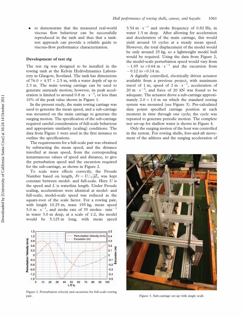
A digitally controlled, electrically driven actuator

available from a previous project, with maximum

travel of 1 m, speed of 2 m � s71, acceleration of

20 m � s72, and force of 20 kN was found to be

adequate. The actuator drove a sub-carriage approxi-

mately 2.06 1.0 m on which the standard towing

system was mounted (see Figure 3). Pre-calculated

data points specified carriage position at each

moment in time through one cycle; the cycle was

repeated to generate periodic motion. The complete

test set-up for shallow water is shown in Figure 4.

Only the surging motion of the boat was controlled

in the system. For rowing shells, fore-and-aft move-

ment of the athletes and the surging acceleration of

Figure 2. Perturbation velocity and excursion for full-scale rowing

pair. Figure 3. Sub-carriage set-up with single scull.

Hull performance of rowing shells, canoes, and kayaks 1061

Dow

nloa

ded

by [

Uni

vers

ity o

f C

alif

orni

a Sa

nta

Cru

z] a

t 16:

24 1

4 O

ctob

er 2

011

the boat lead to a pitching motion, while vertical

acceleration of the athletes and oars leads to a

heaving motion. In the current system, these motions

were not controlled; nonetheless, the boat could

heave and pitch freely due to the varying hydro-

dynamic forces.

Where the focus of testing is on measurement of

unsteady hydrodynamic forces, inertial forces be-

come extremely important. These are typically an

order of magnitude larger than the steady hydro-

dynamic forces, and possibly two orders of magni-

tude larger than unsteady effects. Hence the force

measurement system had to be highly sensitive,

linear, and repeatable, and both the acceleration

and the hull mass had to be measured extremely

precisely.

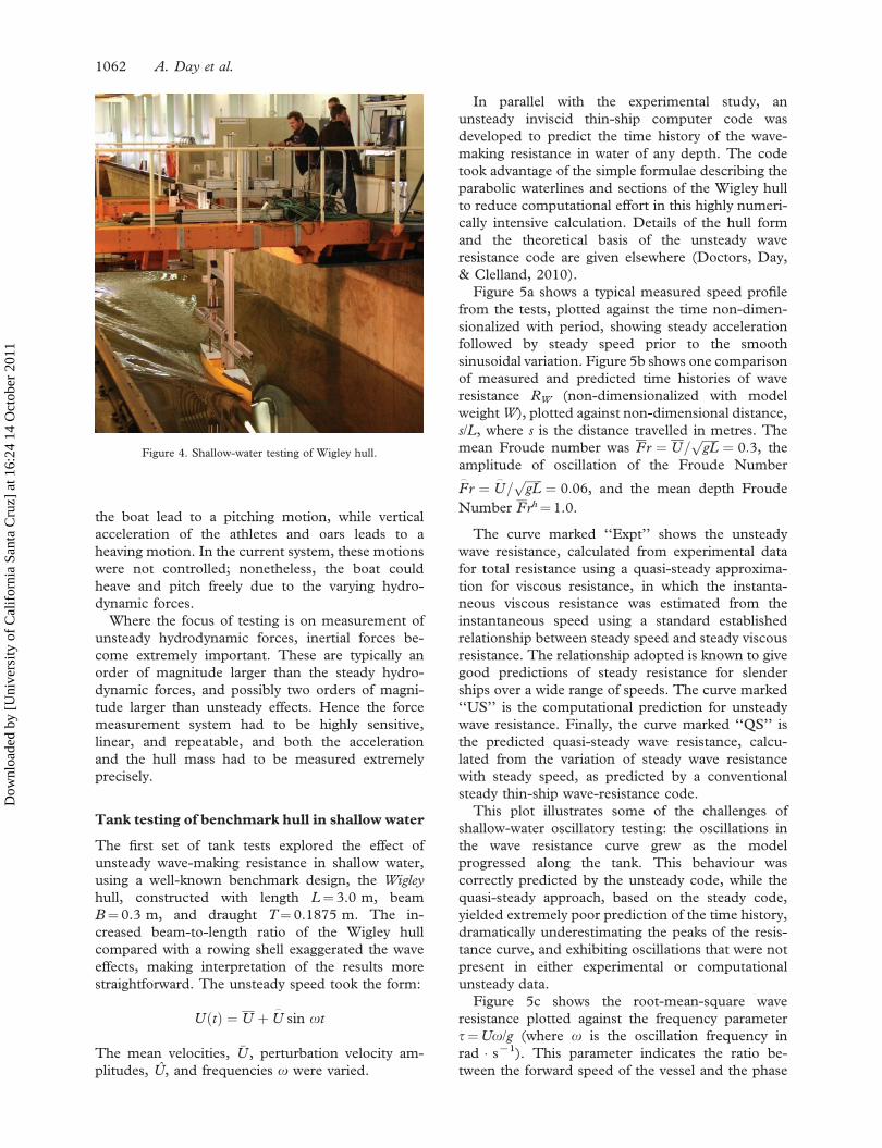
Tank testing of benchmark hull in shallow water

The first set of tank tests explored the effect of

unsteady wave-making resistance in shallow water,

using a well-known benchmark design, the Wigley

hull, constructed with length L¼ 3.0 m, beam

B¼ 0.3 m, and draught T¼ 0.1875 m. The in-

creased beam-to-length ratio of the Wigley hull

compared with a rowing shell exaggerated the wave

effects, making interpretation of the results more

straightforward. The unsteady speed took the form:

UðtÞ ¼ U þU_

sin ot

The mean velocities, �U , perturbation velocity am-

plitudes, U, and frequencies o were varied.

In parallel with the experimental study, an

unsteady inviscid thin-ship computer code was

developed to predict the time history of the wave-

making resistance in water of any depth. The code

took advantage of the simple formulae describing the

parabolic waterlines and sections of the Wigley hull

to reduce computational effort in this highly numeri-

cally intensive calculation. Details of the hull form

and the theoretical basis of the unsteady wave

resistance code are given elsewhere (Doctors, Day,

& Clelland, 2010).

Figure 5a shows a typical measured speed profile

from the tests, plotted against the time non-dimen-

sionalized with period, showing steady acceleration

followed by steady speed prior to the smooth

sinusoidal variation. Figure 5b shows one comparison

of measured and predicted time histories of wave

resistance RW (non-dimensionalized with model

weight W), plotted against non-dimensional distance,

s/L, where s is the distance travelled in metres. The

mean Froude number was Fr ¼ U=ffiffiffiffiffiffi

gLp

¼ 0:3, the

amplitude of oscillation of the Froude Number

F_

r ¼ U_

=ffiffiffiffiffiffi

gLp

¼ 0:06, and the mean depth Froude

Number Frh¼ 1.0.

The curve marked ‘‘Expt’’ shows the unsteady

wave resistance, calculated from experimental data

for total resistance using a quasi-steady approxima-

tion for viscous resistance, in which the instanta-

neous viscous resistance was estimated from the

instantaneous speed using a standard established

relationship between steady speed and steady viscous

resistance. The relationship adopted is known to give

good predictions of steady resistance for slender

ships over a wide range of speeds. The curve marked

‘‘US’’ is the computational prediction for unsteady

wave resistance. Finally, the curve marked ‘‘QS’’ is

the predicted quasi-steady wave resistance, calcu-

lated from the variation of steady wave resistance

with steady speed, as predicted by a conventional

steady thin-ship wave-resistance code.

This plot illustrates some of the challenges of

shallow-water oscillatory testing: the oscillations in

the wave resistance curve grew as the model

progressed along the tank. This behaviour was

correctly predicted by the unsteady code, while the

quasi-steady approach, based on the steady code,

yielded extremely poor prediction of the time history,

dramatically underestimating the peaks of the resis-

tance curve, and exhibiting oscillations that were not

present in either experimental or computational

unsteady data.

Figure 5c shows the root-mean-square wave

resistance plotted against the frequency parameter

t¼Uo/g (where o is the oscillation frequency in

rad � s71). This parameter indicates the ratio be-

tween the forward speed of the vessel and the phase

Figure 4. Shallow-water testing of Wigley hull.

1062 A. Day et al.

Dow

nloa

ded

by [

Uni

vers

ity o

f C

alif

orni

a Sa

nta

Cru

z] a

t 16:

24 1

4 O

ctob

er 2

011

speed of the waves generated by the oscillation

(in deep water). The value at t¼ 0 indicates the

corresponding steady-speed value. It can be seen that

over much of this range, the unsteady value was

substantially higher than the steady-speed value. The

substantial ‘‘hump’’ in the graph around t¼ 0.16 was

well predicted by the theory.

In general, good agreement was found at low mean

speeds and oscillation frequencies between the

unsteady shallow-water wave-resistance computa-

tions and the values derived from tank tests. It could

thus be inferred that the effects of shallow water on

unsteady wave-making resistance was correctly pre-

dicted using the computational approach in these

conditions.

Since the tank-derived values of wave resistance

relied on the quasi-steady approximation to frictional

resistance, it can also be inferred that in these

conditions the viscous resistance was well predicted

by this approximation. In contrast, there was very

poor agreement between tank-derived values for

unsteady wave resistance and predicted quasi-steady

approximation for wave resistance.

However, subsequent tests at higher mean speeds

and with higher values of the frequency parameter,

closer to those experienced in rowing and/or kayaking

races, did not show such good agreement. The data

for Figure 6 were obtained with Fr¼ 0.5, F_

r¼ 0.1,

and Frh¼ 1.0; it can be seen that the trends were

poorly predicted for t4 0.7. Much higher values than

this of the frequency parameter are found in rowing

races; for example, the data shown in Figure 1

correspond to Fr¼ 0.498, F_

r¼ 0.09(þ), F_

r¼0.15(7), and t¼ 1.86. At these higher frequencies,

the measured resistance was found to be substantially

greater than that predicted using the computational

approach, suggesting that the approach was breaking

down in conditions relevant to rowing.

The unsteady wave-resistance calculation, how-

ever, made no assumptions about speed or frequency

except a common linearization that wave steepness

was small. Hence, the approach should in principle

also have behaved well at higher speeds and

frequencies, unless wave behaviour changed drama-

tically in some way. This could have resulted from

Figure 5. Selected results for benchmark tests at low speed and low

frequency. (a) Typical speed profile. (b) Measured and predicted

wave resistance. (c) Measured and predicted root-mean-square

(RMS) wave resistance.

Figure 6. Root-mean-square (RMS) wave resistance for Wigley

hull at moderate speed and frequency.

Hull performance of rowing shells, canoes, and kayaks 1063

Dow

nloa

ded

by [

Uni

vers

ity o

f C

alif

orni

a Sa

nta

Cru

z] a

t 16:

24 1

4 O

ctob

er 2

011

wave-breaking; however, video recordings showed

no evidence of this.

A more likely corollary is that the quasi-steady

approximation for the viscous resistance was failing

in these conditions, and that viscous resistance

increased substantially with higher speed and fre-

quency. One possible contributor to this was the

influence of acceleration on turbulence in the

boundary layer and in particular on the transition

between laminar and turbulent flow. Predicting the

location of the laminar–turbulent transition from first

principles is a hugely challenging problem in ship

resistance prediction even in steady flow; in unsteady

flows of the type of interest here, there is virtually no

information available.

The location of laminar–turbulent transition is

known to be of great practical relevance in hull design

optimization; designing bow shapes to delay transi-

tion is a key strategy for resistance reduction in

yachts, and has been extensively investigated by

America’s Cup technical teams. A preliminary

indication of the importance of the location of

laminar–turbulent transition in the present context

was given by steady-speed tests with transition

‘‘forced’’ at different locations by a girth-wise line of

small studs fitted to the surface of the hull. For the

single scull used here, the steady resistance between

2.5 and 4.0 m � s71 was found to be around 0.5%

higher on average with studs located 400 mm from

the bow compared with the studs located 600 mm

from the bow.

The second phase of the study thus focused on

unsteady effects on laminar–turbulent transition. As

well as providing insight into unsteady effects on

viscous flow, transition provided a useful metric for

the comparison of laboratory and field-trial data for

validation purposes. Total hull resistance would have

been the ideal choice, but was impractical due to the

challenges associated with the measurement of hull

resistance in the field with suitable accuracy.

Field measurement of viscous flow

A series of field trials was carried out with the twin

objectives of establishing realistic speed profiles

for reproduction in the tank, and providing field

measurements against which the test-tank data could

be validated to demonstrate that realistic viscous flow

could be created in the absence of the athlete.

A single scull was chosen for these trials because it

could be tested at full-scale in the tank, hence

avoiding scaling issues for this preliminary study.

Three series of field trials were carried out, in varying

conditions and locations, allowing progressive re-

finement of the systems, and also allowing the rower

to become accustomed to the reduced stability of the

hull resulting from the installed equipment.

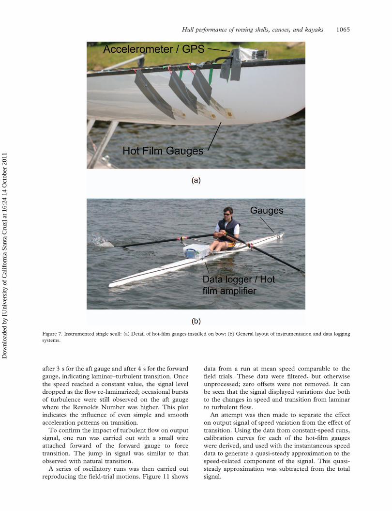
The scull was fitted with conventional hot-film

anemometry gauges (Dantec Dynamics Ltd., Bristol,

UK) in a number of different locations. In the early

sets of tests, several gauges were set up to identify

suitable locations on the hull (see Figure 7a); as runs

progressed, forward gauges were removed to allow

undisturbed flow to gauges further aft. In the final set

of tests, one gauge was located on each side in the

best positions identified to ensure no interference

between the gauges.

Motions were recorded using an integrated system

designed for logging race-car data (VBox 3i, Race-

logic, Buckingham, UK); this comprised GPS to

capture mean speed, accelerometers to obtain surge

and pitch motions, and a portable data logger

including analogue inputs used here to gather the

hot-film data. The data logger and hot-film ampli-

fiers were mounted in a waterproof box aft of the foot

stretcher, as shown in Figure 7b.

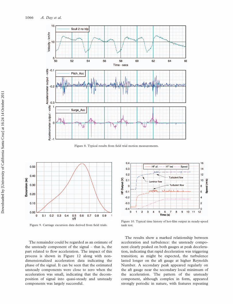
Several runs were made during each set of trials;

each run included some ‘‘cruising’’ strokes, some

‘‘racing’’ strokes, and also a ‘‘coast-down’’ period, in

which the scull decelerated smoothly in a natural

manner. A sample of measured motion data from the

field trials is shown in Figure 8.

The present study focused on the flow behaviour

at the faster stroke rate; a representative cycle was

chosen with maximum speed of 4.4 m � s71. The

time history from the trials motion was then used to

create an input file for the sub-carriage drive system.

The resulting time history of position is shown in

Figure 9.

Towing-tank measurement of viscous flow

The second set of tank tests also focused on the

measurement of turbulence near the bow of a full-

scale single scull. The scull used was similar, but not

identical, to that used in the field trials. Hot-film

gauges were applied in positions similar to those used

in the final set of field trials, at 400 mm and 600 mm

aft of the bow.

A hot-film signal can be characterized as consisting

of four main components: a DC signal that varies

non-linearly with speed; a DC signal that is higher

for turbulent flow than for laminar flow; an AC signal

representing flow turbulence; and intermittency

when the flow is sometimes laminar and sometimes

turbulent.

A series of runs was first carried out at steady

speed to test the hot-film measurements. The data

were filtered with a low-pass digital filter with a cut-

off of 20 Hz to remove electrical noise. Figure 10

shows a time history of a typical run.

The non-linear variation of hot-film signal with

speed can be seen between 1 and 3 s. Jumps of around

0.5 V in the hot-film signals can be observed at just

1064 A. Day et al.

Dow

nloa

ded

by [

Uni

vers

ity o

f C

alif

orni

a Sa

nta

Cru

z] a

t 16:

24 1

4 O

ctob

er 2

011

after 3 s for the aft gauge and after 4 s for the forward

gauge, indicating laminar–turbulent transition. Once

the speed reached a constant value, the signal level

dropped as the flow re-laminarized; occasional bursts

of turbulence were still observed on the aft gauge

where the Reynolds Number was higher. This plot

indicates the influence of even simple and smooth

acceleration patterns on transition.

To confirm the impact of turbulent flow on output

signal, one run was carried out with a small wire

attached forward of the forward gauge to force

transition. The jump in signal was similar to that

observed with natural transition.

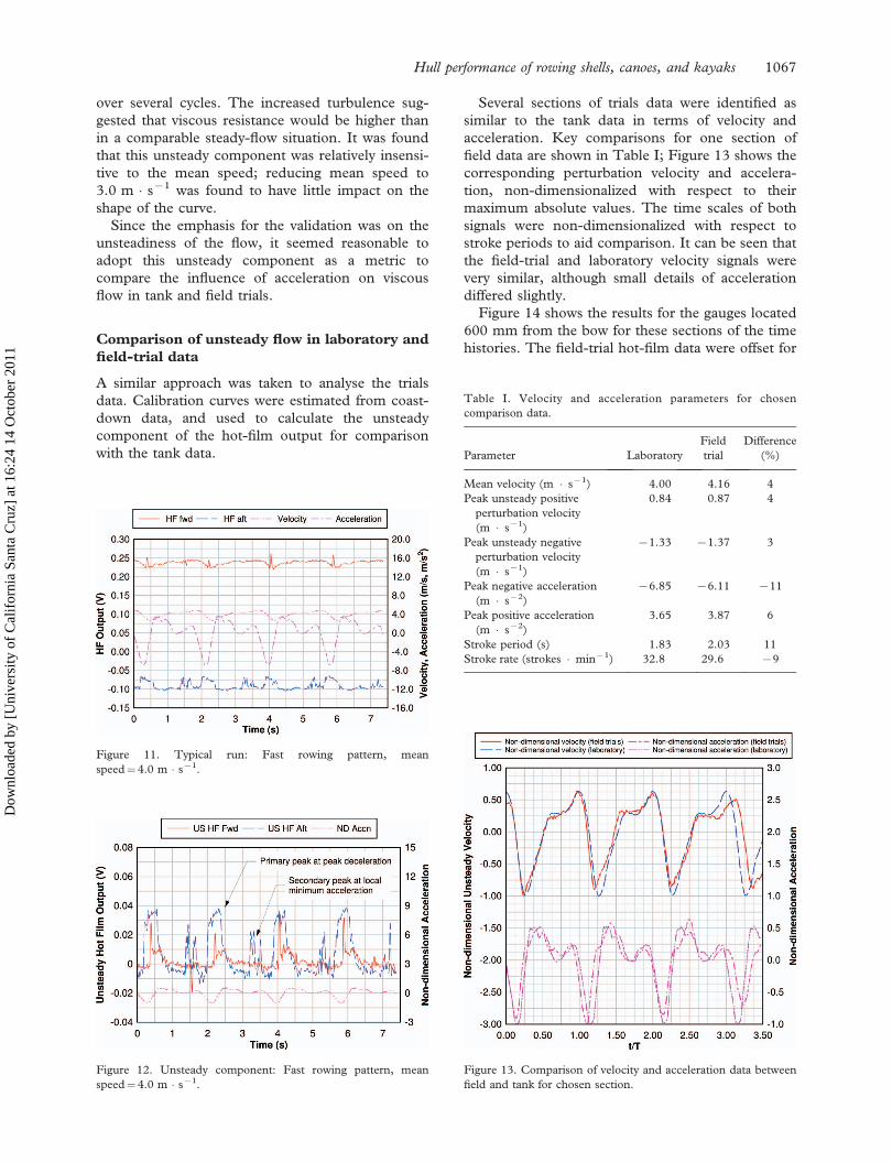
A series of oscillatory runs was then carried out

reproducing the field-trial motions. Figure 11 shows

data from a run at mean speed comparable to the

field trials. These data were filtered, but otherwise

unprocessed; zero offsets were not removed. It can

be seen that the signal displayed variations due both

to the changes in speed and transition from laminar

to turbulent flow.

An attempt was then made to separate the effect

on output signal of speed variation from the effect of

transition. Using the data from constant-speed runs,

calibration curves for each of the hot-film gauges

were derived, and used with the instantaneous speed

data to generate a quasi-steady approximation to the

speed-related component of the signal. This quasi-

steady approximation was subtracted from the total

signal.

Figure 7. Instrumented single scull: (a) Detail of hot-film gauges installed on bow; (b) General layout of instrumentation and data logging

systems.

Hull performance of rowing shells, canoes, and kayaks 1065

Dow

nloa

ded

by [

Uni

vers

ity o

f C

alif

orni

a Sa

nta

Cru

z] a

t 16:

24 1

4 O

ctob

er 2

011

The remainder could be regarded as an estimate of

the unsteady component of the signal – that is, the

part related to flow acceleration. The impact of this

process is shown in Figure 12 along with non-

dimensionalized acceleration data indicating the

phase of the signal. It can be seen that the estimated

unsteady components were close to zero when the

acceleration was small, indicating that the decom-

position of signal into quasi-steady and unsteady

components was largely successful.

The results show a marked relationship between

acceleration and turbulence: the unsteady compo-

nent clearly peaked on both gauges at peak decelera-

tion, indicating that rapid deceleration was triggering

transition; as might be expected, the turbulence

lasted longer on the aft gauge at higher Reynolds

Number. A secondary peak appeared regularly on

the aft gauge near the secondary local minimum of

the acceleration. The pattern of the unsteady

component, although complex in form, appeared

strongly periodic in nature, with features repeating

Figure 8. Typical results from field trial motion measurements.

Figure 9. Carriage excursion data derived from field trials.

Figure 10. Typical time history of hot-film output in steady-speed

tank test.

1066 A. Day et al.

Dow

nloa

ded

by [

Uni

vers

ity o

f C

alif

orni

a Sa

nta

Cru

z] a

t 16:

24 1

4 O

ctob

er 2

011

over several cycles. The increased turbulence sug-

gested that viscous resistance would be higher than

in a comparable steady-flow situation. It was found

that this unsteady component was relatively insensi-

tive to the mean speed; reducing mean speed to

3.0 m � s71 was found to have little impact on the

shape of the curve.

Since the emphasis for the validation was on the

unsteadiness of the flow, it seemed reasonable to

adopt this unsteady component as a metric to

compare the influence of acceleration on viscous

flow in tank and field trials.

Comparison of unsteady flow in laboratory and

field-trial data

A similar approach was taken to analyse the trials

data. Calibration curves were estimated from coast-

down data, and used to calculate the unsteady

component of the hot-film output for comparison

with the tank data.

Several sections of trials data were identified as

similar to the tank data in terms of velocity and

acceleration. Key comparisons for one section of

field data are shown in Table I; Figure 13 shows the

corresponding perturbation velocity and accelera-

tion, non-dimensionalized with respect to their

maximum absolute values. The time scales of both

signals were non-dimensionalized with respect to

stroke periods to aid comparison. It can be seen that

the field-trial and laboratory velocity signals were

very similar, although small details of acceleration

differed slightly.

Figure 14 shows the results for the gauges located

600 mm from the bow for these sections of the time

histories. The field-trial hot-film data were offset for

Figure 11. Typical run: Fast rowing pattern, mean

speed¼4.0 m � s71.

Figure 12. Unsteady component: Fast rowing pattern, mean

speed¼4.0 m � s71.

Table I. Velocity and acceleration parameters for chosen

comparison data.

Parameter Laboratory

Field

trial

Difference

(%)

Mean velocity (m � s71) 4.00 4.16 4

Peak unsteady positive

perturbation velocity

(m � s71)

0.84 0.87 4

Peak unsteady negative

perturbation velocity

(m � s71)

71.33 71.37 3

Peak negative acceleration

(m � s72)

76.85 76.11 711

Peak positive acceleration

(m � s72)

3.65 3.87 6

Stroke period (s) 1.83 2.03 11

Stroke rate (strokes � min71) 32.8 29.6 79

Figure 13. Comparison of velocity and acceleration data between

field and tank for chosen section.

Hull performance of rowing shells, canoes, and kayaks 1067

Dow

nloa

ded

by [

Uni

vers

ity o

f C

alif

orni

a Sa

nta

Cru

z] a

t 16:

24 1

4 O

ctob

er 2

011

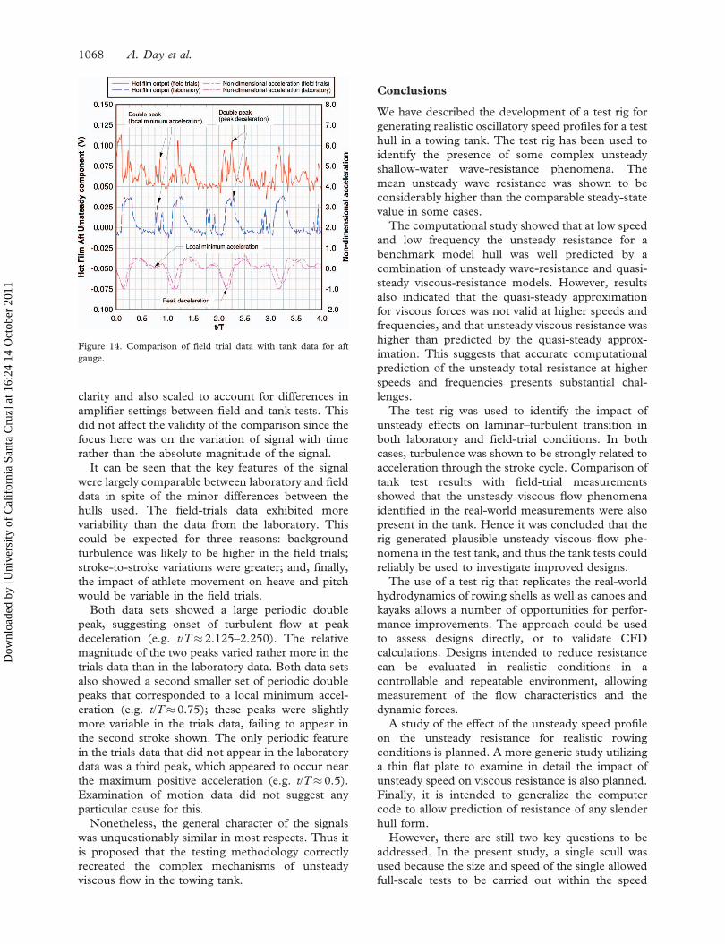
clarity and also scaled to account for differences in

amplifier settings between field and tank tests. This

did not affect the validity of the comparison since the

focus here was on the variation of signal with time

rather than the absolute magnitude of the signal.

It can be seen that the key features of the signal

were largely comparable between laboratory and field

data in spite of the minor differences between the

hulls used. The field-trials data exhibited more

variability than the data from the laboratory. This

could be expected for three reasons: background

turbulence was likely to be higher in the field trials;

stroke-to-stroke variations were greater; and, finally,

the impact of athlete movement on heave and pitch

would be variable in the field trials.

Both data sets showed a large periodic double

peak, suggesting onset of turbulent flow at peak

deceleration (e.g. t/T� 2.125–2.250). The relative

magnitude of the two peaks varied rather more in the

trials data than in the laboratory data. Both data sets

also showed a second smaller set of periodic double

peaks that corresponded to a local minimum accel-

eration (e.g. t/T� 0.75); these peaks were slightly

more variable in the trials data, failing to appear in

the second stroke shown. The only periodic feature

in the trials data that did not appear in the laboratory

data was a third peak, which appeared to occur near

the maximum positive acceleration (e.g. t/T� 0.5).

Examination of motion data did not suggest any

particular cause for this.

Nonetheless, the general character of the signals

was unquestionably similar in most respects. Thus it

is proposed that the testing methodology correctly

recreated the complex mechanisms of unsteady

viscous flow in the towing tank.

Conclusions

We have described the development of a test rig for

generating realistic oscillatory speed profiles for a test

hull in a towing tank. The test rig has been used to

identify the presence of some complex unsteady

shallow-water wave-resistance phenomena. The

mean unsteady wave resistance was shown to be

considerably higher than the comparable steady-state

value in some cases.

The computational study showed that at low speed

and low frequency the unsteady resistance for a

benchmark model hull was well predicted by a

combination of unsteady wave-resistance and quasi-

steady viscous-resistance models. However, results

also indicated that the quasi-steady approximation

for viscous forces was not valid at higher speeds and

frequencies, and that unsteady viscous resistance was

higher than predicted by the quasi-steady approx-

imation. This suggests that accurate computational

prediction of the unsteady total resistance at higher

speeds and frequencies presents substantial chal-

lenges.

The test rig was used to identify the impact of

unsteady effects on laminar–turbulent transition in

both laboratory and field-trial conditions. In both

cases, turbulence was shown to be strongly related to

acceleration through the stroke cycle. Comparison of

tank test results with field-trial measurements

showed that the unsteady viscous flow phenomena

identified in the real-world measurements were also

present in the tank. Hence it was concluded that the

rig generated plausible unsteady viscous flow phe-

nomena in the test tank, and thus the tank tests could

reliably be used to investigate improved designs.

The use of a test rig that replicates the real-world

hydrodynamics of rowing shells as well as canoes and

kayaks allows a number of opportunities for perfor-

mance improvements. The approach could be used

to assess designs directly, or to validate CFD

calculations. Designs intended to reduce resistance

can be evaluated in realistic conditions in a

controllable and repeatable environment, allowing

measurement of the flow characteristics and the

dynamic forces.

A study of the effect of the unsteady speed profile

on the unsteady resistance for realistic rowing

conditions is planned. A more generic study utilizing

a thin flat plate to examine in detail the impact of

unsteady speed on viscous resistance is also planned.

Finally, it is intended to generalize the computer

code to allow prediction of resistance of any slender

hull form.

However, there are still two key questions to be

addressed. In the present study, a single scull was

used because the size and speed of the single allowed

full-scale tests to be carried out within the speed

Figure 14. Comparison of field trial data with tank data for aft

gauge.

1068 A. Day et al.

Dow

nloa

ded

by [

Uni

vers

ity o

f C

alif

orni

a Sa

nta

Cru

z] a

t 16:

24 1

4 O

ctob

er 2

011

limitations of the test tank. Even so, only a small

number of oscillation cycles was possible at full

speed. To test faster hulls, scale models would be

required. Froude similarity would then lead to lower

model-scale speed, and higher model-scale fre-

quency, and hence more oscillations in the scope of

the tank, but further validation would be required to

understand the scaling of the unsteady viscous

effects.

Finally, to complete the accuracy of the modelling,

it would also be desirable to build a mechanism to

replicate the complete six-degree-of-freedom mo-

tions. It is likely that heave and pitch would be

dominant in rowing applications in which power is

applied in a symmetrical fashion, while roll and yaw

would also be important in canoe/kayak applications

due to the asymmetry of the power application.

Acknowledgements

This work was funded by the UK Engineering and

Physical Sciences Research Council (EPSRC) under

the ‘‘Achieving Gold’’ programme grants EP/

F006284/1 and EP/F00625X/1. Prof. Doctors’ par-

ticipation in the benchmark study was also supported

by EPSRC under grant EP/F019998/1. We are

indebted to Charles Keay and the technical staff of

the Kelvin Hydrodynamics Lab for constructing the

test rig, and assisting with all aspects of the tank-test

programme

References

Berton, M., Alessandrini, B., Barre, S., & Kobus, J. M. (2007).

Verification and validation in computational fluid dynamics:

Application to both steady and unsteady rowing boats

numerical simulations. In Proceedings of the 17th International

Offshore and Polar Engineering Conference (pp. 2006–2011).

Mountain View, CA: International Society of Offshore and

Polar Engineers.

Bugalski, T. J. (2009). Development of the new line of sprint

canoes for the Olympic Games. In Proceedings of the 10th

International Conference on Fast Sea Transportation (FAST 2009)

(pp. 1039–1049). Athens: FAST Organizing Committee.

Doctors, L. J., Day, A. H., & Clelland, D. (2010). Resistance of a

ship undergoing oscillatory motion. Journal of Ship Research, 54

(2), 120–132.

Faltinsen, O. M. (2005). Hydrodynamics of high-speed marine

vehicles. Cambridge: Cambridge University Press.

Formaggia, L., Miglio, E., Mola, A., & Montano, A. (2009). A

model for the dynamics of rowing boats. International Journal for

Numerical Methods in Fluids, 61, 119–143.

Formaggia, L., Miglio, E., Mola, A., & Parolini, N. (2008). Fluid–

structure interaction problems in free surface flows: Application

to boat dynamics. International Journal for Numerical Methods in

Fluids, 56, 965–978.

Kleshnev, V. (2002). Rowing Biomechanics Newsletter, 2 (6).

Lazauskas, L. (1998). Rowing shell drag comparisons. Technical

report L9701, Department of Mathematics, University of

Adelaide. Retrieved from: http://www.cyberiad.net/library/

rowing/real/realrow.htm.

Lazauskas, L., & Tuck, E. O. (1996). Low drag racing kayaks.

Technical report, Department of Mathematics, University of

Adelaide. Retrieved from: http://www.cyberiad.net/library/

kayaks/racing/racing.htm.

Lazauskas, L., & Winters, J. (1997). Hydrodynamic drag of some

small sprint kayaks. Technical report, Department of Mathe-

matics, University of Adelaide. Retrieved from: http://www.

cyberiad.net/library/kayaks/jwsprint/jwsprint.htm.

Scragg, C. A., & Nelson, B. D. (1993). The design of an eight-

oared rowing shell. Marine Technology, 30 (2), 84–99.

Tuck, E. O., & Lazauskas, L. (1996). Low drag rowing shells. In

Proceedings of the 3rd Conference on Mathematics and Computers in

Sport (pp. 17–34). Robina, QLD: Bond University.

Wellicome, J. F. (1967). Report on resistance experiments carried out

on three racing shells. National Physical Laboratory Ship T.M.

184.

Hull performance of rowing shells, canoes, and kayaks 1069

Dow

nloa

ded

by [

Uni

vers

ity o

f C

alif

orni

a Sa

nta

Cru

z] a

t 16:

24 1

4 O

ctob

er 2

011