Real-time Trajectory Design for Unmanned Aerial

Vehicles using Receding Horizon Control

by

Yoshiaki Kuwata

Bachelor of EngineeringThe University of Tokyo, 2001

Submitted to the Department of Aeronautics and Astronautics

in partial fulfillment of the requirements for the degree of

Master of Science in Aeronautics and Astronautics

at the

MASSACHUSETTS INSTITUTE OF TECHNOLOGY

June 2003

c© Yoshiaki Kuwata, MMIII. All rights reserved.

The author hereby grants to MIT permission to reproduce

and distribute publicly paper and electronic copiesof this thesis document in whole or in part.

Author . . . . . . . . . . . . . . . . . . . . . . . . . . . . . . . . . . . . . . . . . . . . . . . . . . . . . . . . . . . . . . . . . . . .

Department of Aeronautics and AstronauticsMay 23, 2003

Certified by . . . . . . . . . . . . . . . . . . . . . . . . . . . . . . . . . . . . . . . . . . . . . . . . . . . . . . . . . . . . . . .

Jonathan P. HowAssociate Professor

Thesis Supervisor

Accepted by . . . . . . . . . . . . . . . . . . . . . . . . . . . . . . . . . . . . . . . . . . . . . . . . . . . . . . . . . . . . . . .Edward M. Greitzer

H.N. Slater Professor of Aeronautics and Astronautics

Chair, Committee on Graduate Students

2

Real-time Trajectory Design for Unmanned Aerial Vehicles using

Receding Horizon Control

by

Yoshiaki Kuwata

Submitted to the Department of Aeronautics and Astronauticson May 23, 2003, in partial fulfillment of the

requirements for the degree ofMaster of Science in Aeronautics and Astronautics

Abstract

This thesis investigates the coordination and control of fleets of unmanned aerial vehicles(UAVs). Future UAVs will operate autonomously, and their control systems must com-pensate for significant dynamic uncertainty. A hierarchical approach has been proposedto account for various types of uncertainty at different levels of the control system. Theresulting controller includes task assignment, graph-based coarse path planning, detailedtrajectory optimization using receding horizon control (RHC), and a low-level waypoint fol-lower. Mixed-integer linear programming (MILP) is applied to both the task allocation andtrajectory design problems to encode logical constraints and discrete decisions together withthe continuous vehicle dynamics.The MILP RHC uses a simple vehicle dynamics model in the near term and an approxi-

mate path model in the long term. This combination gives a good estimate of the cost-to-goand greatly reduces the computational effort required to design the complete trajectory, butdiscrepancies in the assumptions made in the two models can lead to infeasible solutions.The primary contribution of this thesis is to extend the previous stable RHC formulationto ensure that the on-line optimizations will always be feasible. Novel pruning and graph-search algorithms are also integrated with the MILP RHC, and the resulting controller isanalytically shown to guarantee finite-time arrival at the goal. This pruning algorithm alsosignificantly reduces the computational load of the MILP RHC.The control algorithms acting on four different levels of the hierarchy were integrated

and tested on two hardware testbeds (three small ground vehicles and a hardware-in-the-loop simulation of three aircraft autopilots) to verify real-time operation in the presence ofreal-world disturbances and uncertainties. Experimental results show the successful controlloop closures in various scenarios, including operation with restricted environment knowledgebased on a realistic sensor and a coordinated mission by different types of UAVs.

Thesis Supervisor: Jonathan P. HowTitle: Associate Professor

3

4

Acknowledgments

I would like to thank several people who made this research possible. First, my advisor

Professor Jonathan How guided me through this work with a lot of insight. This research is

an extension of John Bellingham’s work. Many inputs from Arthur Richards are appreciated.

The hardware experiments could not be performed without the help of Chung Tin, Ian

Garcia, and Ellis King. I would also like to thank Louis Breger, Mehdi Alighanbari, Luca

Bertuccelli, and Megan Mitchell for their support through the ordeal. Last but not least,

administrative assistant Margaret Yoon helped notably to put the final touches on this thesis.

This research was funded under DARPA contract # N66001-01-C-8075. The testbeds

described in Chapter 5 of the thesis were funded under the DURIP grant (AFOSR Grant

# F49620-02-1-0216).

5

6

Contents

1 Introduction 17

1.1 Background . . . . . . . . . . . . . . . . . . . . . . . . . . . . . . . . . . . . 17

1.1.1 Trajectory Design . . . . . . . . . . . . . . . . . . . . . . . . . . . . 18

1.1.2 Task Allocation . . . . . . . . . . . . . . . . . . . . . . . . . . . . . 20

1.2 Thesis Overview . . . . . . . . . . . . . . . . . . . . . . . . . . . . . . . . . 20

2 Receding Horizon Control using Mixed-Integer Linear Programming 23

2.1 Overview of the Receding Horizon Controller . . . . . . . . . . . . . . . . . 23

2.2 Model of Aircraft Dynamics . . . . . . . . . . . . . . . . . . . . . . . . . . . 25

2.2.1 Discrete Time System . . . . . . . . . . . . . . . . . . . . . . . . . . 25

2.2.2 Speed Constraints . . . . . . . . . . . . . . . . . . . . . . . . . . . . 26

2.2.3 Minimum Turning Radius . . . . . . . . . . . . . . . . . . . . . . . . 28

2.3 Collision Avoidance Constraints . . . . . . . . . . . . . . . . . . . . . . . . 30

2.3.1 Obstacle Avoidance . . . . . . . . . . . . . . . . . . . . . . . . . . . 30

2.3.2 Vehicle Avoidance . . . . . . . . . . . . . . . . . . . . . . . . . . . . 32

2.4 Plan beyond the Planning Horizon . . . . . . . . . . . . . . . . . . . . . . . 33

2.5 Target Visit . . . . . . . . . . . . . . . . . . . . . . . . . . . . . . . . . . . . 35

2.6 Cost Function . . . . . . . . . . . . . . . . . . . . . . . . . . . . . . . . . . 37

2.7 Example . . . . . . . . . . . . . . . . . . . . . . . . . . . . . . . . . . . . . 39

2.8 Conclusions . . . . . . . . . . . . . . . . . . . . . . . . . . . . . . . . . . . . 42

7

3 Stable Receding Horizon Trajectory Designer 43

3.1 Overview . . . . . . . . . . . . . . . . . . . . . . . . . . . . . . . . . . . . . 44

3.2 Visibility Graph . . . . . . . . . . . . . . . . . . . . . . . . . . . . . . . . . 45

3.3 Modified Dijkstra’s Algorithm . . . . . . . . . . . . . . . . . . . . . . . . . . 46

3.3.1 Turning Circles Around a Corner . . . . . . . . . . . . . . . . . . . . 47

3.3.2 Modified Dijkstra’s Algorithm . . . . . . . . . . . . . . . . . . . . . 55

3.4 Cost Points . . . . . . . . . . . . . . . . . . . . . . . . . . . . . . . . . . . . 58

3.4.1 Corner Selection . . . . . . . . . . . . . . . . . . . . . . . . . . . . . 58

3.4.2 Effect on the Computation Time . . . . . . . . . . . . . . . . . . . . 60

3.5 Stability Proof . . . . . . . . . . . . . . . . . . . . . . . . . . . . . . . . . . 63

3.5.1 Stability Criteria . . . . . . . . . . . . . . . . . . . . . . . . . . . . . 63

3.5.2 Finite Time Completion . . . . . . . . . . . . . . . . . . . . . . . . . 68

3.6 Conclusions . . . . . . . . . . . . . . . . . . . . . . . . . . . . . . . . . . . . 72

4 Task allocation for Multiple UAVs with Timing Constraints and Loitering 75

4.1 Problem Formulation . . . . . . . . . . . . . . . . . . . . . . . . . . . . . . 75

4.1.1 Problem Statement . . . . . . . . . . . . . . . . . . . . . . . . . . . 76

4.1.2 Algorithm Overview . . . . . . . . . . . . . . . . . . . . . . . . . . . 76

4.1.3 Decision Variables . . . . . . . . . . . . . . . . . . . . . . . . . . . . 77

4.1.4 Timing Constraints . . . . . . . . . . . . . . . . . . . . . . . . . . . 80

4.1.5 Cost Function . . . . . . . . . . . . . . . . . . . . . . . . . . . . . . 81

4.2 Simulation Results . . . . . . . . . . . . . . . . . . . . . . . . . . . . . . . . 81

4.2.1 Problem With and Without Timing Constraints . . . . . . . . . . . 81

4.2.2 Complexity of Adding Timing Constraints . . . . . . . . . . . . . . . 84

4.3 Conclusions . . . . . . . . . . . . . . . . . . . . . . . . . . . . . . . . . . . . 87

5 Hardware Experiments 89

5.1 Experiments Overview . . . . . . . . . . . . . . . . . . . . . . . . . . . . . . 89

5.2 Hardware Setup . . . . . . . . . . . . . . . . . . . . . . . . . . . . . . . . . 92

8

5.2.1 Interface Setup . . . . . . . . . . . . . . . . . . . . . . . . . . . . . . 92

5.2.2 Truck Testbed . . . . . . . . . . . . . . . . . . . . . . . . . . . . . . 93

5.2.3 UAV Testbed . . . . . . . . . . . . . . . . . . . . . . . . . . . . . . . 97

5.3 Receding Horizon Controller with Low-Level Feedback Controller . . . . . . 99

5.3.1 On-line Replanning Concept . . . . . . . . . . . . . . . . . . . . . . 99

5.3.2 Scenario . . . . . . . . . . . . . . . . . . . . . . . . . . . . . . . . . . 101

5.4 On-line Trajectory Regeneration . . . . . . . . . . . . . . . . . . . . . . . . 106

5.4.1 Obstacle Detection . . . . . . . . . . . . . . . . . . . . . . . . . . . . 106

5.4.2 Collision Avoidance Maneuver . . . . . . . . . . . . . . . . . . . . . 116

5.5 On-Line Task Reassignment . . . . . . . . . . . . . . . . . . . . . . . . . . . 126

5.5.1 Scenario Description . . . . . . . . . . . . . . . . . . . . . . . . . . . 130

5.5.2 Demonstration . . . . . . . . . . . . . . . . . . . . . . . . . . . . . . 132

5.6 Conclusions . . . . . . . . . . . . . . . . . . . . . . . . . . . . . . . . . . . . 141

6 Conclusions and Future Work 143

6.1 Contributions . . . . . . . . . . . . . . . . . . . . . . . . . . . . . . . . . . . 143

6.2 Future Research Directions . . . . . . . . . . . . . . . . . . . . . . . . . . . 145

9

10

List of Figures

1-1 Block diagram of the hierarchical approach developed in this thesis. . . . . 21

2-1 Projection of velocity vector . . . . . . . . . . . . . . . . . . . . . . . . . . 26

2-2 Convex and non-convex constraints on a normalized velocity vector . . . . 28

2-3 Turn with the maximum acceleration . . . . . . . . . . . . . . . . . . . . . 30

2-4 Corner cut and obstacle expansion . . . . . . . . . . . . . . . . . . . . . . . 32

2-5 Step over of thin obstacle . . . . . . . . . . . . . . . . . . . . . . . . . . . . 32

2-6 Safety distance for vehicle collision avoidance in relative frame . . . . . . . 33

2-7 Line-of-sight vector and cost-to-go . . . . . . . . . . . . . . . . . . . . . . . 37

2-8 Trajectory with minimum speed constraints . . . . . . . . . . . . . . . . . 40

2-9 Trajectory without minimum speed constraints . . . . . . . . . . . . . . . . 40

2-10 History of speed . . . . . . . . . . . . . . . . . . . . . . . . . . . . . . . . . 41

2-11 Computation time for simple example . . . . . . . . . . . . . . . . . . . . . 41

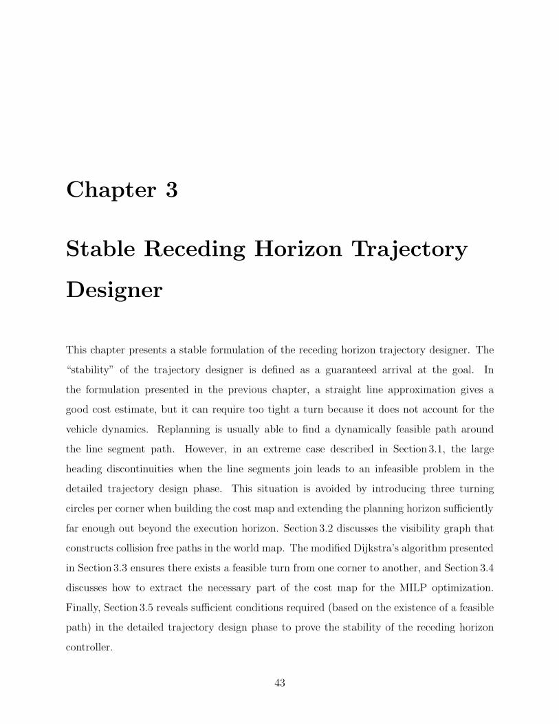
3-1 Straight line approximation goes through the narrow passage . . . . . . . . 44

3-2 Infeasible problem in the detailed trajectory design phase . . . . . . . . . . 44

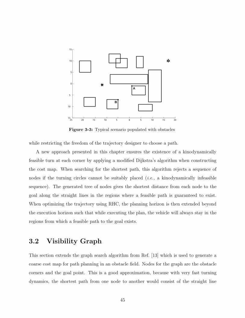
3-3 Typical scenario populated with obstacles . . . . . . . . . . . . . . . . . . . 45

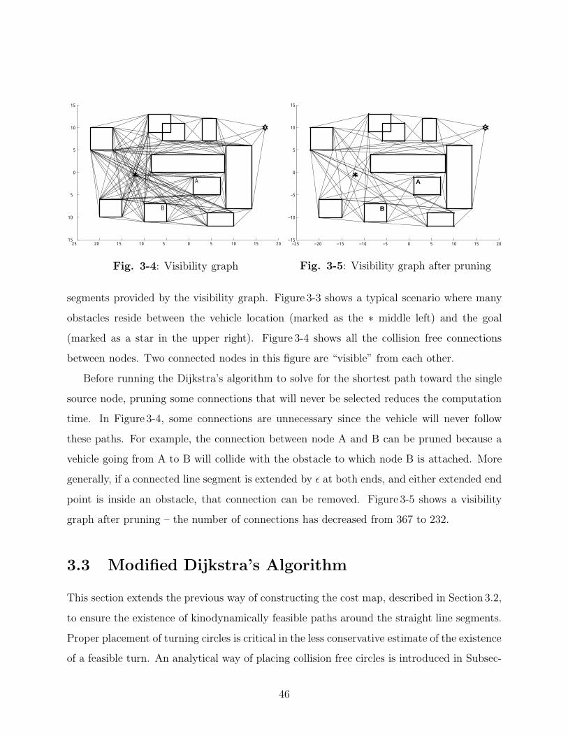
3-4 Visibility graph . . . . . . . . . . . . . . . . . . . . . . . . . . . . . . . . . 46

3-5 Visibility graph after pruning . . . . . . . . . . . . . . . . . . . . . . . . . 46

3-6 Three turning circles at obstacle corner . . . . . . . . . . . . . . . . . . . . 47

3-7 Circle placement problem . . . . . . . . . . . . . . . . . . . . . . . . . . . . 48

3-8 Two cases for determining horizontal distance . . . . . . . . . . . . . . . . 49

11

3-9 Two cases for determining comeback point depending on separation distance 51

3-10 Two cases for determining the center O0 of circle C0 . . . . . . . . . . . . . 52

3-11 Angles used in the calculation of the centers of circles . . . . . . . . . . . . 53

3-12 Two cases for determining the center O2 of circle C2 . . . . . . . . . . . . . 54

3-13 Tree of shortest paths . . . . . . . . . . . . . . . . . . . . . . . . . . . . . . 57

3-14 Precedence of cost points . . . . . . . . . . . . . . . . . . . . . . . . . . . . 59

3-15 Points visible from the initial position . . . . . . . . . . . . . . . . . . . . . 61

3-16 Points visible and connectable from the initial position . . . . . . . . . . . 61

3-17 Cost points used in MILP . . . . . . . . . . . . . . . . . . . . . . . . . . . 61

3-18 Trajectory in the highly constrained environment . . . . . . . . . . . . . . 62

3-19 Comparison of the computation times . . . . . . . . . . . . . . . . . . . . . 62

3-20 Minimum margin to keep execution horizon in a feasible region . . . . . . . 64

3-21 Worst case turn . . . . . . . . . . . . . . . . . . . . . . . . . . . . . . . . . 67

3-22 Trajectory . . . . . . . . . . . . . . . . . . . . . . . . . . . . . . . . . . . . 70

3-23 Decrease of cost-to-go . . . . . . . . . . . . . . . . . . . . . . . . . . . . . . 70

3-24 Selection of another path . . . . . . . . . . . . . . . . . . . . . . . . . . . . 71

4-1 Flight time, loiter time, time of arrival, and time of task execution . . . . . 79

4-2 Scenario with 6 heterogenous UAVs & 12 waypoints (No timing constraints) 82

4-3 Scenario with 6 heterogenous UAVs & 12 waypoints (7 timing constraints) 82

4-4 Scenario with 6 heterogenous UAVs & 12 waypoints (11 timing constraints) 82

4-5 TOE i ≥ TOE j . . . . . . . . . . . . . . . . . . . . . . . . . . . . . . . . . . 85

4-6 TOE i ≥ TOE j + 10 . . . . . . . . . . . . . . . . . . . . . . . . . . . . . . . 85

4-7 TOE i ≥ TOE j ≥ TOE k . . . . . . . . . . . . . . . . . . . . . . . . . . . . . 85

4-8 TOE i ≥ TOE j + 5 ≥ TOE k + 10 . . . . . . . . . . . . . . . . . . . . . . . . 85

5-1 Loop closure at different levels . . . . . . . . . . . . . . . . . . . . . . . . . 90

5-2 Planner and hardware integration . . . . . . . . . . . . . . . . . . . . . . . 92

5-3 Truck testbed . . . . . . . . . . . . . . . . . . . . . . . . . . . . . . . . . . 94

12

5-4 Truck testbed system diagram . . . . . . . . . . . . . . . . . . . . . . . . . 94

5-5 Waypoint following method for truck testbed . . . . . . . . . . . . . . . . . 95

5-6 Heading control loop . . . . . . . . . . . . . . . . . . . . . . . . . . . . . . 96

5-7 Root locus of the heading controller . . . . . . . . . . . . . . . . . . . . . . 96

5-8 Speed control loop . . . . . . . . . . . . . . . . . . . . . . . . . . . . . . . 97

5-9 Root locus of the speed controller . . . . . . . . . . . . . . . . . . . . . . . 97

5-10 PT40 Aircrafts . . . . . . . . . . . . . . . . . . . . . . . . . . . . . . . . . 98

5-11 Autopilot . . . . . . . . . . . . . . . . . . . . . . . . . . . . . . . . . . . . 98

5-12 Autopilot testbed system diagram . . . . . . . . . . . . . . . . . . . . . . . 98

5-13 Distance travelled and elapsed time . . . . . . . . . . . . . . . . . . . . . . 100

5-14 Complex scenario for one vehicle . . . . . . . . . . . . . . . . . . . . . . . . 101

5-15 Planned waypoints and actual position data of truck . . . . . . . . . . . . . 103

5-16 Computation time . . . . . . . . . . . . . . . . . . . . . . . . . . . . . . . . 104

5-17 Trajectory of plan number 13 . . . . . . . . . . . . . . . . . . . . . . . . . 104

5-18 Speed profile . . . . . . . . . . . . . . . . . . . . . . . . . . . . . . . . . . . 105

5-19 Computation time of the planner with the improved pruning algorithm . . 105

5-20 Scenario and trajectory based on full knowledge of the environment. . . . . 107

5-21 Detection of an obstacle with previously known shape. . . . . . . . . . . . 108

5-22 Estimation of an obstacle with an optimistic view of the world. . . . . . . 109

5-23 Estimation of an obstacle with a pessimistic view of the world. . . . . . . . 111

5-24 Planned waypoints and actual trajectory of the truck . . . . . . . . . . . . 113

5-25 Computation time for obstacle detection scenario . . . . . . . . . . . . . . 115

5-26 Collision avoidance maneuver with naive cost-to-go. . . . . . . . . . . . . . 117

5-27 Collision avoidance maneuver with improved cost-to-go . . . . . . . . . . . 120

5-28 Cost-to-go in relative frame, no adjustment of in-track position . . . . . . . 122

5-29 Actual position data in absolute frame . . . . . . . . . . . . . . . . . . . . 123

5-30 Adjustment of in-track position for the next optimization. . . . . . . . . . 124

5-31 Cost-to-go in relative frame, with adjustment of in-track position . . . . . . 125

13

5-32 Adjustment of in-track position in relative frame . . . . . . . . . . . . . . . 126

5-33 Actual position data in absolute frame . . . . . . . . . . . . . . . . . . . . 127

5-34 Cost-to-go in relative frame, with adjustment of in-track position . . . . . . 128

5-35 Case–3. Cost-to-go in relative frame, with adjustment of in-track position.

Actual position data in absolute frame is shown. . . . . . . . . . . . . . . . 129

5-36 Scenario with tightly coupled tasks . . . . . . . . . . . . . . . . . . . . . . 132

5-37 Scenario 1: Vehicle 3 updates the position of HVT A . . . . . . . . . . . . 134

5-38 Scenario 1: Vehicle 3 updates the position of HVT B . . . . . . . . . . . . 134

5-39 Scenario 1: Vehicle 1 detects a new obstacle . . . . . . . . . . . . . . . . . 134

5-40 Planned waypoints and actual UAV trajectories for Scenario 1 . . . . . . . 135

5-41 Scenario 2: Vehicle 3 discovers that strike on HVT A is unsuccessful . . . . 136

5-42 Scenario 2: Vehicle 3 assesses HVT A again . . . . . . . . . . . . . . . . . 136

5-43 Planned waypoints and actual UAV trajectories for Scenario 2 . . . . . . . 137

5-44 Scenario 3: Sudden loss of vehicle 2 . . . . . . . . . . . . . . . . . . . . . . 138

5-45 Scenario 3: Vehicle 1 comes all the way back . . . . . . . . . . . . . . . . . 138

5-46 Planned waypoints and actual UAV trajectories for Scenario 3 . . . . . . . 139

5-47 Computation time of each plan for the three scenarios . . . . . . . . . . . . 140

14

List of Tables

2.1 Minimum turn radii . . . . . . . . . . . . . . . . . . . . . . . . . . . . . . . 30

3.1 Difference ∆J in the distance . . . . . . . . . . . . . . . . . . . . . . . . . . 53

3.2 Minimum margin . . . . . . . . . . . . . . . . . . . . . . . . . . . . . . . . . 65

4.1 Results with no constraints on loitering time. . . . . . . . . . . . . . . . . . 84

4.2 Result with constrained loitering times. . . . . . . . . . . . . . . . . . . . . 84

5.1 Types of each target . . . . . . . . . . . . . . . . . . . . . . . . . . . . . . . 131

5.2 Timing constraints for the scenario . . . . . . . . . . . . . . . . . . . . . . . 131

15

16

Chapter 1

Introduction

1.1 Background

The capabilities and roles of unmanned aerial vehicles (UAVs) are evolving, and new concepts

are required for their control [1]. For example, today’s UAVs typically require several opera-

tors per aircraft, but future UAVs will be designed to make tactical decisions autonomously

and will be integrated into coordinated teams to achieve high-level goals, thereby allowing

one operator to control a group of vehicles. Thus, new methods in planning and execution

are required to coordinate the operation of a fleet of UAVs. An overall control system ar-

chitecture must also be developed that can perform optimal coordination of the vehicles,

evaluate the overall system performance in real time, and quickly reconfigure to account for

changes in the environment or the fleet. This thesis presents results on the guidance and

control of fleets of cooperating UAVs, including goal assignment, trajectory optimization,

and hardware experiments.

For many vehicles, obstacles, and targets, fleet coordination is a very complicated opti-

mization problem [1, 2, 3] where computation time increases very rapidly with the problem

size. Ref. [4] proposed an approach to decompose this large problem into assignment and tra-

jectory problems, while capturing key features of the coupling between them. This allows the

control architecture to solve an allocation problem first to determine a sequence of waypoints

17

for each vehicle to visit, and then concentrate on designing paths to visit these pre-assigned

waypoints. Since the assignment is based on a reasonable estimate of the trajectories, this

separation causes a minimal degradation in the overall performance.

1.1.1 Trajectory Design

Optimizing a kinematically and dynamically constrained path is a significant problem in

controlling autonomous vehicles, and has received attention in the fields of robotics, un-

dersea vehicles, and aerial vehicles [5, 6]. Planning trajectories that are both optimal and

dynamically feasible is complicated by the fact that the space of possible control actions is

extremely large and non-convex, and that simplifications reducing the dimensionality of the

problem without losing feasibility and optimality are very difficult to achieve.

Previous work demonstrated the use of mixed-integer linear programming (MILP) in

off-line trajectory design for vehicles under various dynamic and kinematic constraints [7,

8, 9]. MILP allows the inclusion of non-convex constraints and discrete decisions in the

trajectory optimization. Binary decision variables allow the choice of whether to pass “left”

or “right” of an obstacle, for example, or the discrete assignment of vehicles to targets to be

included in the planning problem. Optimal solutions can be obtained for these trajectory

generation problems using commercially available software such as CPLEX [10, 11]. Using

MILP, however, to design a whole trajectory with a planning horizon fixed at the goal is

very difficult to perform in real time because the computational effort required grows rapidly

with the length of the route and the number of obstacles to be avoided.

This limitation can be avoided by using a receding planning horizon in which MILP is

used to form a shorter plan that extends towards the goal, but does not necessarily reach

it. This overall approach is known as either model predictive control (MPC) or receding

horizon control (RHC) [12]. The performance of a RHC strongly depends on the proper

evaluation of the terminal penalty on the shorter plan. This evaluation is difficult when

the feasibility of the path beyond the plan must be ensured. Previous work presented a

heuristic to approximate the trajectory beyond the shorter plan that used straight line paths

18

to estimate the cost-to-go from the plan’s end point to the goal [3, 13, 14]. This RHC makes

full use of the future states predicted through a model in order to obtain the current control

inputs. In a trajectory design problem, the future states can be predicted by the straight

line paths. This is because the shortest path from any location to the goal is a connection of

straight lines, if no vehicle dynamics are involved and no disturbances act on the vehicle. As

such, generating a coarse cost map based on straight line approximations (and then using

Dijkstra’s algorithm) provides a good prediction of the future route beyond the planning

horizon. The receding horizon controller designs a detailed trajectory over the planning

horizon by evaluating the terminal state with this cost map.

While this planner provides good results in practice, the trajectory design problem can

become infeasible when the positioning of nearby obstacles leaves no dynamically feasible

trajectory from the state that is to be reached by the vehicle. This is because the Dijkstra’s

algorithm neglects the vehicle dynamics when constructing the cost map. In such a case, the

vehicle cannot follow the heading discontinuities where the line segments intersect since the

path associated with the cost-to-go estimate is not dynamically feasible.

This thesis presents one way to overcome the issues with the previous RHC approach

by evaluating the cost-to-go estimate along straight line paths that are known to be “near”

kinodynamically feasible paths to the goal (see Chapter 3 for details). This new trajectory

designer is shown to: (a) be capable of designing trajectories in highly constrained envi-

ronments, where the formulation presented in Ref. [13] is incapable of reaching the goal;

and (b) travel more aggressively since the turn around an obstacle corner is designed at the

MILP optimization phase, unlike a trajectory designer that allows only predetermined turns

at each corner [15].

Although RHC has been successfully applied to chemical process control [16], applications

to systems with faster dynamics, such as those found in the field of aerospace, have been

impractical until recently. The on-going improvements in computation speed has stimulated

recent hardware work in this field, including the on-line use of nonlinear trajectory generator

(NTG) optimization for control of an aerodynamic system [17, 18]. The use of MILP together

19

with RHC enables the application of the real-time trajectory optimization to scenarios with

multiple ground and aerial vehicles that operate in dynamic environments with obstacles.

1.1.2 Task Allocation

A further key aspect of the UAV problem is the allocation of different tasks to UAVs with

different capabilities [19]. This is essentially a multiple-choice multi-dimension knapsack

problem (MMKP) [20], where the number of possible allocations grows rapidly as the problem

size increases. The situation is further complicated if the tasks:

• Are strongly coupled – e.g., a waypoint must be visited three times, first by a type 1

UAV, followed by a type 2, and then a type 3. These three events must occur within

tl seconds of each other.

• Have tight relative timing constraints – e.g., three UAVs must be assigned to strike a

target from three different directions within 2 seconds of each other.

With limited resources within the team, the coupling and timing constraints can result in

very tight linkages between the activities of the various vehicles. Especially towards the

end of missions, these tend to cause significant problems (e.g., “churning” and/or infeasible

solutions) for the approximate assignment algorithms based on “myopic algorithms” (e.g. it-

erative “greedy” or network flow solutions) that have recently been developed [2, 19]. MILP,

again, provides a natural language for codifying these various mission objectives and con-

straints using a combination of binary (e.g., as switches for the discrete/logical decisions)

and continuous (e.g., for start and arrival time) variables [3, 12, 4]. MILP allows us to ac-

count for the coupling and relative timing constraints and to handle large fleets with many

targets and/or pop-up threats.

1.2 Thesis Overview

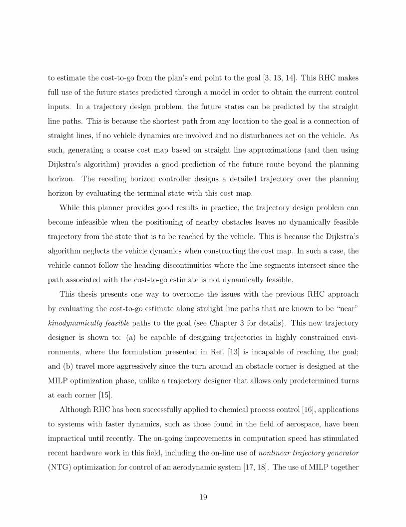
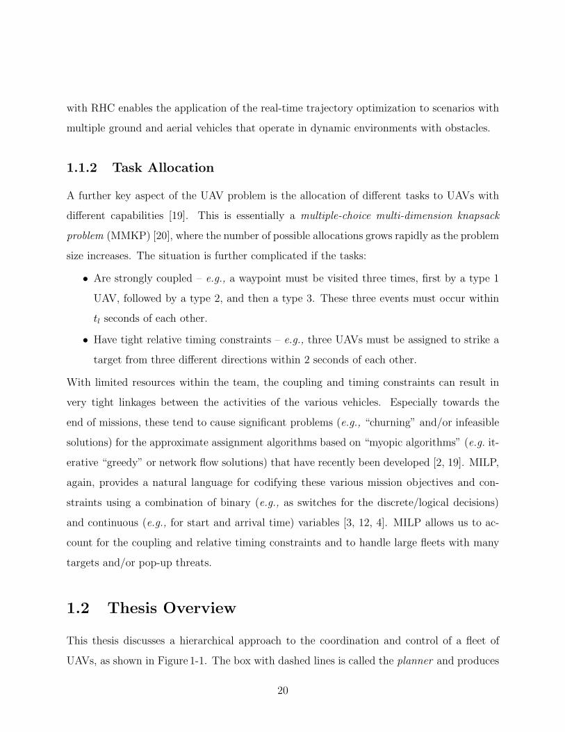
This thesis discusses a hierarchical approach to the coordination and control of a fleet of

UAVs, as shown in Figure 1-1. The box with dashed lines is called the planner and produces

20

actuator inputAssignedtargets

Minimum turn radiusNominal speed

UAVmodel

Vehicle statesObstaclesTargets

Vehicle statesObstacles

controlsignal

e.g.waypoints and activities

Vehicle capabilityNominal speed

Aircraftinertialsensordata

State of the worldPredictor / Comparator

Real world/

Simulation

ObstaclesTargets

Approx. cost

High level

Planner

Mission Req.

Feasible plan

Low level

ControllerTrajectoryDesigner

Graph- based

Path planning

Task Assignment

Chap.Chap. 2,2,

Chap.Chap. 33Chap.Chap. 44

Chap.Chap. 2,2,

Chap.Chap. 33

Chap.Chap. 55

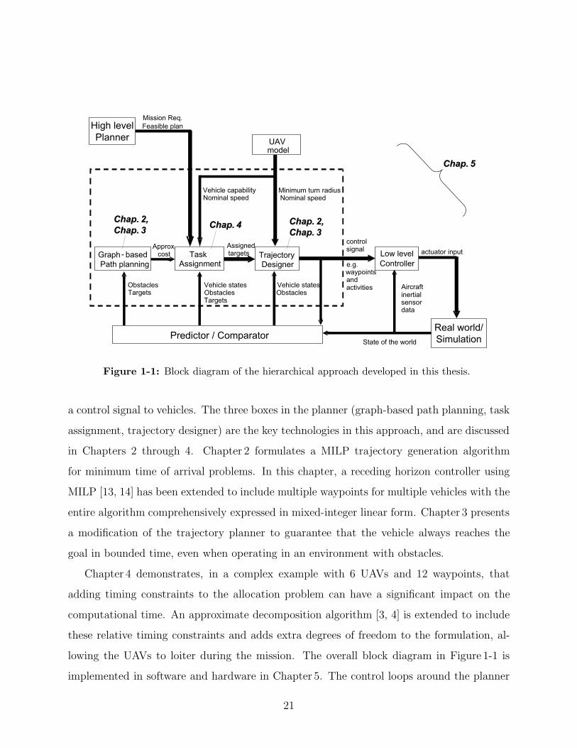
Figure 1-1: Block diagram of the hierarchical approach developed in this thesis.

a control signal to vehicles. The three boxes in the planner (graph-based path planning, task

assignment, trajectory designer) are the key technologies in this approach, and are discussed

in Chapters 2 through 4. Chapter 2 formulates a MILP trajectory generation algorithm

for minimum time of arrival problems. In this chapter, a receding horizon controller using

MILP [13, 14] has been extended to include multiple waypoints for multiple vehicles with the

entire algorithm comprehensively expressed in mixed-integer linear form. Chapter 3 presents

a modification of the trajectory planner to guarantee that the vehicle always reaches the

goal in bounded time, even when operating in an environment with obstacles.

Chapter 4 demonstrates, in a complex example with 6 UAVs and 12 waypoints, that

adding timing constraints to the allocation problem can have a significant impact on the

computational time. An approximate decomposition algorithm [3, 4] is extended to include

these relative timing constraints and adds extra degrees of freedom to the formulation, al-

lowing the UAVs to loiter during the mission. The overall block diagram in Figure 1-1 is

implemented in software and hardware in Chapter 5. The control loops around the planner

21

are closed one at a time, and several experimental results demonstrate the real-time loop

closures using two new testbeds.

22

Chapter 2

Receding Horizon Control using

Mixed-Integer Linear Programming

This chapter presents several extensions to a previous formulation of a receding horizon

controller for minimum time trajectory generation problems [14]. Section 2.1 addresses the

concept of receding horizon control (RHC) and how it is applied to trajectory optimization

problems. Then, the trajectory optimization problem is formulated usingmixed-integer linear

programming (MILP), which is well suited to trajectory planning because it can directly

incorporate logical constraints such as obstacle avoidance and waypoint selection and because

it provides an optimization framework that can account for basic dynamic constraints such

as turn limitations.

2.1 Overview of the Receding Horizon Controller

Improvements in UAV capabilities make it possible for UAVs to perform longer and more

complicated missions and scenarios. In these missions and scenarios, optimal path navigation

through complicated environments is crucial to mission success. As more vehicles and more

targets are involved in the mission, the complexity of the trajectory design problem grows

rapidly, increasing the computation time to obtain the optimal solution [9]. One alternative

23

to overcome this computational burden is to use receding horizon control (RHC) [21]. The

RHC uses a plant model and an optimization technique to design an input trajectory that

optimizes the plant’s output over a period of time called the planning horizon. A portion

of the input trajectory is then implemented over the shorter execution horizon, and the

optimization is performed again starting from the state that is to be reached. If the control

problem is not completed at the end of the planning horizon, the cost incurred past the

planning horizon must be accounted for in the cost function. The selection of the terminal

penalty in RHC design is a crucial factor in obtaining reasonable performance, especially in

the presence of obstacles and no-fly zones.

In general, the cost function of a receding horizon controller’s optimization problem es-

timates the cost-to-go from a selected terminal state to the goal. For vehicle trajectory

planning problems in a field with no-fly zones, Ref. [13] presented a receding horizon con-

troller that uses the length of a path to the goal made up of straight line segments as its

cost-to-go. This is a good approximation for minimum time of arrival problems since the

true minimum distance path to the goal will typically touch the corners of obstacles that

block the vehicle’s path. In order to connect the detailed trajectory designed over the plan-

ning horizon and the coarse cost map beyond it, the RHC selects an obstacle corner that

is visible from the terminal point and is associated with the best path. This approach has

another advantage in terms of real-time applications. The cost map not only gives a good

prediction of vehicle behavior beyond the planning horizon, but because it is very coarse, it

also can be rapidly updated when the environment and/or situational awareness changes.

The following sections focus on solving the vehicle trajectory design problem after a set

of ordered goals are assigned to each vehicle. The MILP formulation presented here extends

an existing algorithm [13, 14] to incorporate more sophisticated scenarios (e.g., multiple

vehicles, multiple goals) and detailed dynamics (e.g., constant speed operation).

24

2.2 Model of Aircraft Dynamics

It has been shown that the point mass dynamics subject to two-norm constraints form an

approximate model for limited turn-rate vehicles, provided that the optimization favors the

minimum time, or minimum distance, path [9]. By explicitly including minimum speed

constraints, this formulation can be applied to problems with various objectives, such as

expected score and risk, with a minimal increase in computation time.

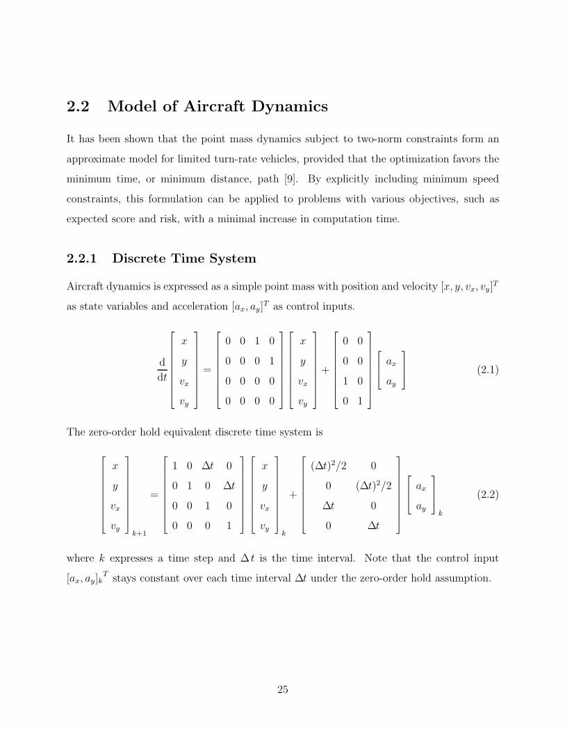
2.2.1 Discrete Time System

Aircraft dynamics is expressed as a simple point mass with position and velocity [x, y, vx, vy]T

as state variables and acceleration [ax, ay]T as control inputs.

d

dt

x

y

vx

vy

=

0 0 1 0

0 0 0 1

0 0 0 0

0 0 0 0

x

y

vx

vy

+

0 0

0 0

1 0

0 1

axay

(2.1)

The zero-order hold equivalent discrete time system is

x

y

vx

vy

k+1

=

1 0 ∆t 0

0 1 0 ∆t

0 0 1 0

0 0 0 1

x

y

vx

vy

k

+

(∆t)2/2 0

0 (∆t)2/2

∆t 0

0 ∆t

axay

k

(2.2)

where k expresses a time step and ∆ t is the time interval. Note that the control input

[ax, ay]kT stays constant over each time interval ∆t under the zero-order hold assumption.

25

v

v · ik

ik

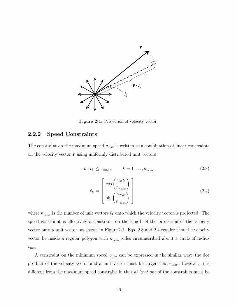
Figure 2-1: Projection of velocity vector

2.2.2 Speed Constraints

The constraint on the maximum speed vmax is written as a combination of linear constraints

on the velocity vector v using uniformly distributed unit vectors

v · ik ≤ vmax, k = 1, . . . , nvmax (2.3)

ik =

cos

(2πk

nvmax

)

sin

(2πk

nvmax

) (2.4)

where nvmax is the number of unit vectors ik onto which the velocity vector is projected. The

speed constraint is effectively a constraint on the length of the projection of the velocity

vector onto a unit vector, as shown in Figure 2-1. Eqs. 2.3 and 2.4 require that the velocity

vector be inside a regular polygon with nvmax sides circumscribed about a circle of radius

vmax.

A constraint on the minimum speed vmin can be expressed in the similar way: the dot

product of the velocity vector and a unit vector must be larger than vmin. However, it is

different from the maximum speed constraint in that at least one of the constraints must be

26

active, instead of all of them,

v · ik ≥ vmin, ∃k, (k = 1, . . . , nvmin) (2.5)

ik =

cos

(2πk

nvmin

)

sin

(2πk

nvmin

) (2.6)

Here, nvminis the number of unit vectors onto which the velocity vector is projected. Eq. 2.5

is a non-convex constraint and is written as a combination of mixed-integer linear constraints

v · ik ≥ vmin −Mv(1− bspeed,k), k = 1, . . . , nvmin(2.7)

nvmin∑k=1

bspeed,k ≥ 1 (2.8)

whereMv is a number larger than 2vmin, and the bspeed,k are binary variables that express the

non-convex constraints in the MILP form. Note that if bspeed,k = 1, the inequality in Eq. 2.7

is active, indicating that the minimum speed constraint is satisfied. On the other hand, if

bspeed,k = 0, the kth constraint in Eq. 2.7 is not active, and the constraint on minimum speed

is relaxed. Eq. 2.8 requires that at least one constraint in Eq. 2.7 be active. Eqs. 2.6 to 2.8

ensure that the tip of the velocity vector lies outside of a regular polygon with nvminsides

circumscribed on the outside of a circle with radius vmin.

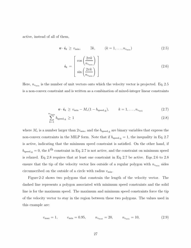
Figure 2-2 shows two polygons that constrain the length of the velocity vector. The

dashed line represents a polygon associated with minimum speed constraints and the solid

line is for the maximum speed. The maximum and minimum speed constraints force the tip

of the velocity vector to stay in the region between these two polygons. The values used in

this example are:

vmax = 1, vmin = 0.95, nvmax = 20, nvmin= 10, (2.9)

27

−1 −0.8 −0.6 −0.4 −0.2 0 0.2 0.4 0.6 0.8 1

−1

−0.8

−0.6

−0.4

−0.2

0

0.2

0.4

0.6

0.8

1 min speedmax speed

Figure 2-2: Convex and non-convex constraints on a normalized velocity vector

Since the minimum speed constraints require binary variables, which typically slows down

the MILP optimization process, nvminis typically much smaller than nvmax . Note that the

speed constraints can become infeasible if vmax and vmin are set equal unless nvmax = nvmin.

In Figure 2-2, for example, if the radius of the dashed polygon is increased, then no feasible

velocity vector exists in the direction [0, 1]T (straight up), because the minimum constraint

will be larger than the maximum constraint.

2.2.3 Minimum Turning Radius

UAVs usually fly at roughly a constant speed v and have a minimum turning radius rmin.

The constraint on the turning radius r is

rmin ≤ r = v2

a(2.10)

28

and this constraint can be written as a constraint on lateral acceleration,

a ≤ v2

rmin≡ amax (2.11)

where a is the magnitude of the acceleration vector and amax is the maximum acceleration

magnitude. Similar to the maximum speed constraint, the constraint on the maximum

acceleration is written as a combination of linear constraints on the acceleration vector a

a · ik ≤ amax, k = 1, . . . , na (2.12)

ik =

cos

(2πk

na

)

sin

(2πk

na

) (2.13)

where na is the number of unit vectors onto which the acceleration vector is projected. The

constraints on velocity in Eqs. 2.3 to 2.8 keep the speed roughly constant, so the allowable

acceleration vector direction is perpendicular to the velocity vector. The state equation

(Eq. 2.2) for the vehicle uses a zero-order hold on the inputs, so the acceleration vector

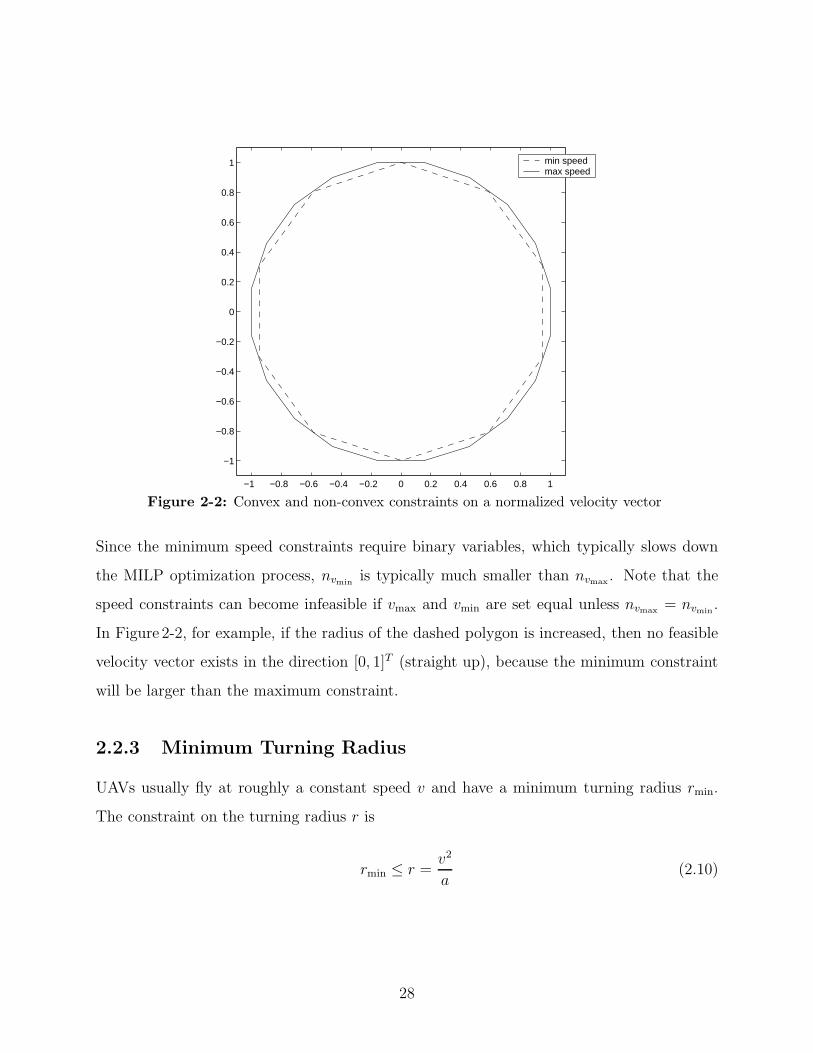
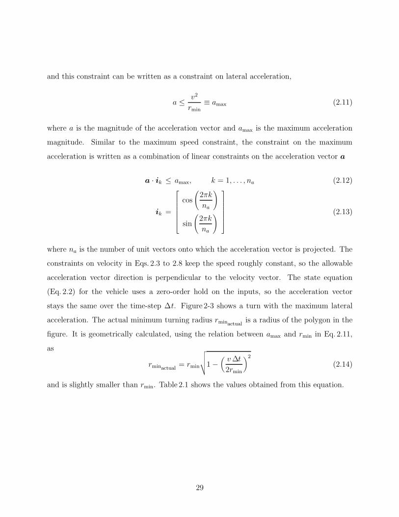
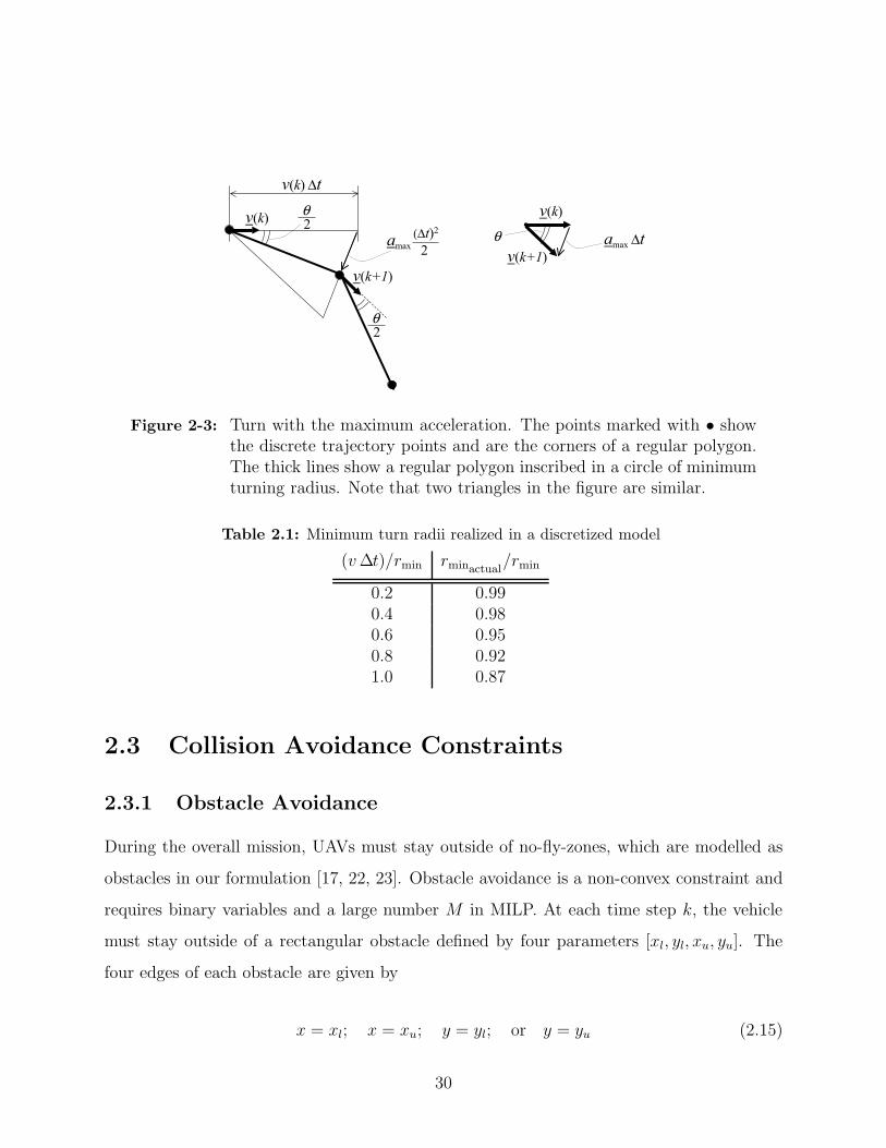
stays the same over the time-step ∆t. Figure 2-3 shows a turn with the maximum lateral

acceleration. The actual minimum turning radius rminactualis a radius of the polygon in the

figure. It is geometrically calculated, using the relation between amax and rmin in Eq. 2.11,

as

rminactual= rmin

√√√√1− (v∆t

2rmin

)2

(2.14)

and is slightly smaller than rmin. Table 2.1 shows the values obtained from this equation.

29

v(k) ∆t

v(k+1)

v(k)

amax

(∆t)2

2

2θ

2θ v(k)

v(k+1)amax ∆tθ

Figure 2-3: Turn with the maximum acceleration. The points marked with • showthe discrete trajectory points and are the corners of a regular polygon.The thick lines show a regular polygon inscribed in a circle of minimumturning radius. Note that two triangles in the figure are similar.

Table 2.1: Minimum turn radii realized in a discretized model

(v∆t)/rmin rminactual/rmin

0.2 0.990.4 0.980.6 0.950.8 0.921.0 0.87

2.3 Collision Avoidance Constraints

2.3.1 Obstacle Avoidance

During the overall mission, UAVs must stay outside of no-fly-zones, which are modelled as

obstacles in our formulation [17, 22, 23]. Obstacle avoidance is a non-convex constraint and

requires binary variables and a large number M in MILP. At each time step k, the vehicle

must stay outside of a rectangular obstacle defined by four parameters [xl, yl, xu, yu]. The

four edges of each obstacle are given by

x = xl; x = xu; y = yl; or y = yu (2.15)

30

The constraints on vehicle position are formulated as

xk ≤ xl +M bobst,1jk (2.16)

yk ≤ yl +M bobst,2jk (2.17)

xk ≥ xu −M bobst,3jk (2.18)

yk ≥ yu −M bobst,4jk (2.19)

4∑i=1

bobst,ijk ≤ 3 (2.20)

j = 1, . . . , no, k = 1, . . . , np

where [xk, yk]T gives the position of a vehicle at time k, M is a number larger than the

size of the world map, no is the number of obstacles, np is the number of steps in the

planning horizon, and bobst,ijk is an i − j − kth element of a binary matrix of size 4 by noby np. At time-step k, if bobst,ijk = 0 in Eqs. 2.16 to 2.19, then the constraint is active and

the vehicle is outside of the jth obstacle. If not, the large number M relaxes the obstacle

avoidance constraint. The logical constraint in Eq. 2.20 requires that at least one of the four

constraints be active for each obstacle at each time-step. The obstacle shape is assumed to

be rectangular, but this formulation is extendable to obstacles with polygonal shapes. Also,

non-convex obstacles can be easily formed by overlapping several rectangular obstacles.

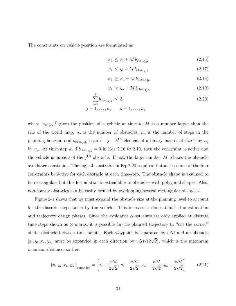
Figure 2-4 shows that we must expand the obstacle size at the planning level to account

for the discrete steps taken by the vehicle. This increase is done at both the estimation

and trajectory design phases. Since the avoidance constraints are only applied at discrete

time steps shown as ⊗ marks, it is possible for the planned trajectory to “cut the corner”

of the obstacle between time points. Each waypoint is separated by v∆t and an obstacle

[xl, yl, xu, yu] must be expanded in each direction by v∆ t/(2√2), which is the maximum

incursion distance, so that

[xl, yl, xu, yu]∣∣∣expanded

=

[xl − v∆t

2√2, yl − v∆t

2√2, xu +

v∆t

2√2, yu +

v∆t

2√2

](2.21)

31

vdt

Actual

Obstacle

Figure 2-4: Corner cut and obstacle expansion

v dt

wmin

Figure 2-5: Step over of thin obstacle

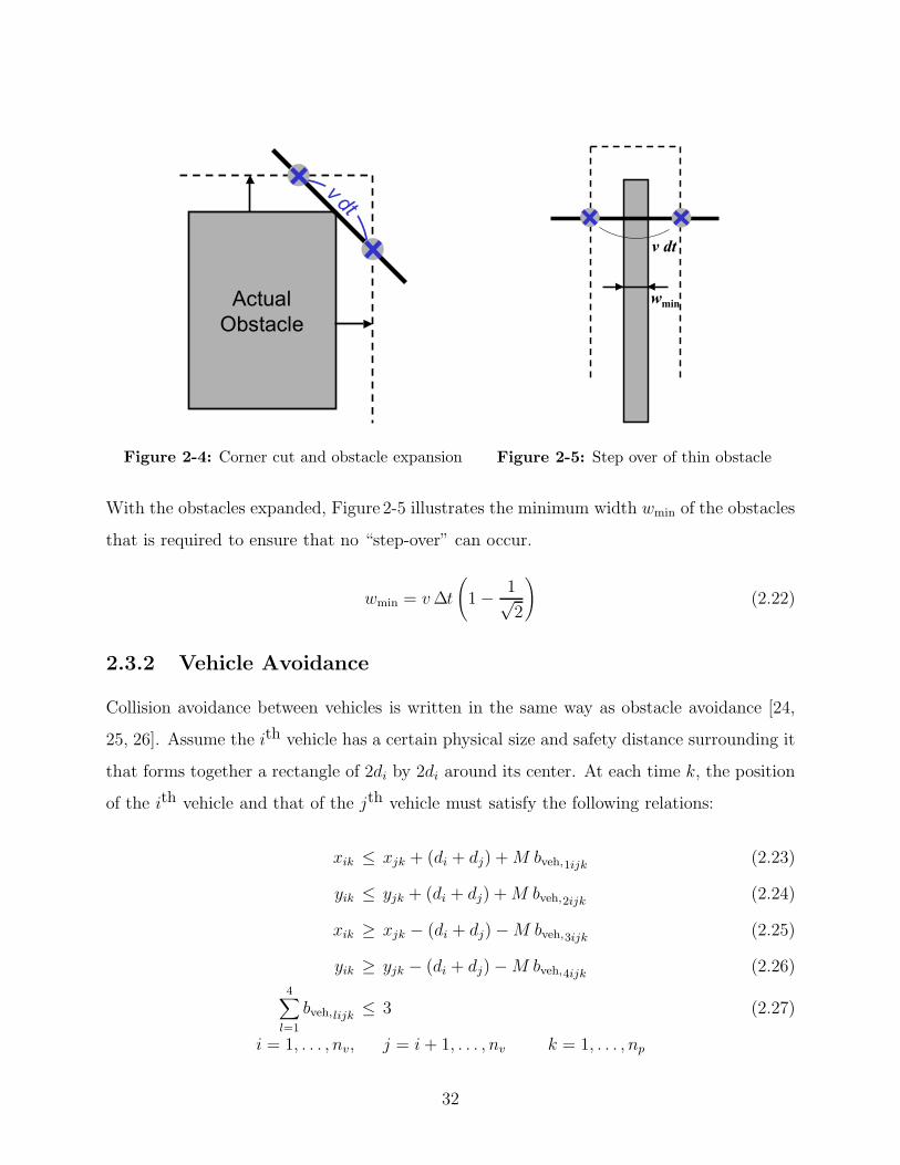
With the obstacles expanded, Figure 2-5 illustrates the minimum width wmin of the obstacles

that is required to ensure that no “step-over” can occur.

wmin = v∆t

(1− 1√

2

)(2.22)

2.3.2 Vehicle Avoidance

Collision avoidance between vehicles is written in the same way as obstacle avoidance [24,

25, 26]. Assume the ith vehicle has a certain physical size and safety distance surrounding it

that forms together a rectangle of 2di by 2di around its center. At each time k, the position

of the ith vehicle and that of the jth vehicle must satisfy the following relations:

xik ≤ xjk + (di + dj) +M bveh,1ijk (2.23)

yik ≤ yjk + (di + dj) +M bveh,2ijk (2.24)

xik ≥ xjk − (di + dj)−M bveh,3ijk (2.25)

yik ≥ yjk − (di + dj)−M bveh,4ijk (2.26)

4∑l=1

bveh,lijk ≤ 3 (2.27)

i = 1, . . . , nv, j = i+ 1, . . . , nv k = 1, . . . , np

32

(vi + v

j ) dt

di+ dj

di+ dj

Figure 2-6: Safety distance for vehicle collision avoidance in relative frame

where [xik, yik]T gives the position of a vehicle i at time k, nv is the number of vehicles, and

bveh,lijk is the l − i − j − kth element of a binary matrix of size 4 by nv by nv by np. Ifbveh,lijk = 0 in Eqs. 2.23 to 2.26, the constraint is active, and the safety boxes of the two

vehicles, i and j, do not intersect each other.

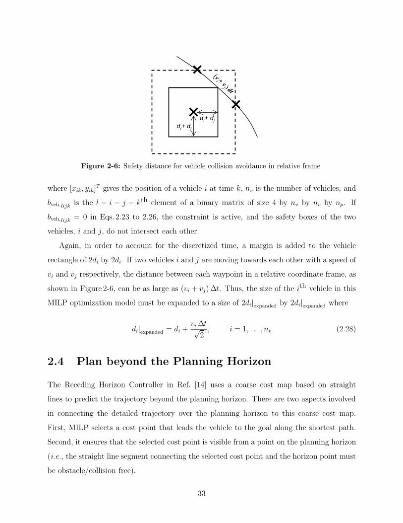
Again, in order to account for the discretized time, a margin is added to the vehicle

rectangle of 2di by 2di. If two vehicles i and j are moving towards each other with a speed of

vi and vj respectively, the distance between each waypoint in a relative coordinate frame, as

shown in Figure 2-6, can be as large as (vi + vj)∆t. Thus, the size of the ith vehicle in this

MILP optimization model must be expanded to a size of 2di|expanded by 2di|expanded where

di|expanded = di +vi∆t√2, i = 1, . . . , nv (2.28)

2.4 Plan beyond the Planning Horizon

The Receding Horizon Controller in Ref. [14] uses a coarse cost map based on straight

lines to predict the trajectory beyond the planning horizon. There are two aspects involved

in connecting the detailed trajectory over the planning horizon to this coarse cost map.

First, MILP selects a cost point that leads the vehicle to the goal along the shortest path.

Second, it ensures that the selected cost point is visible from a point on the planning horizon

(i.e., the straight line segment connecting the selected cost point and the horizon point must

be obstacle/collision free).

33

Given the location of the obstacles and a goal, the cost points are defined as the obsta-

cle corners and the goal itself. The shortest distance from a cost point to the goal along

kinematically feasible straight-line segments forms a cost associated with the cost point and

goal. If a cost point is inside of another obstacle, it has an infinite cost.

Let [xcp,i, ycp,i]T denote the ith cost point, ci the cost associated with the ith cost point,

and cvis,k the cost-to-go at the cost point selected by vehicle k. The binary variables associ-

ated with cost point selection bcp will have three dimensions for cost point, goal, and vehicle,

where nc is a number of cost points, and ng is a number of goals:

cvis,k =nc∑i=1

ng∑j=1

ci bcp,ijk (2.29)

nc∑i=1

ng∑j=1

bcp,ijk = 1, k = 1, . . . , nv (2.30)

Eq. 2.30 enforces the constraint that each vehicle must choose a combination of goal and cost

point, and Eq. 2.29 extracts the cost-to-go at the selected point from the cost map ci.

In order to ensure that the selected cost point [xvis,k, yvis,k]T is visible from the terminal

point [(xnp)k, (ynp)k]T of vehicle k, obstacle avoidance is checked at nt test points that are

placed on a line segment connecting the two points. This requires binary variables bvis

that have four dimensions: the obstacle corner, vehicle, test point, and obstacle. The test

conditions can be written as:

xvis,k

yvis,k

= nc∑

i=1

ng∑j=1

xcp,k

ycp,k

bcp,ijk (2.31)

xLOS,k

yLOS,k

=

xvis,k

yvis,k

−

(xnp)k

(ynp)k

(2.32)

xtest,km

ytest,km

=

(xnp)k

(ynp)k

+ m

nt

xLOS,k

yLOS,k

(2.33)

xtest,km ≤ (xl)n +M bvis,1kmn (2.34)

ytest,km ≤ (yl)n +M bvis,2kmn (2.35)

34

xtest,km ≥ (xu)n −M bvis,3kmn (2.36)

ytest,km ≥ (yu)n −M bvis,4kmn (2.37)4∑

i=1

bvis,ikmn ≤ 3 (2.38)

k = 1, . . . , nv, m = 1, . . . , nt, n = 1, . . . , no

where [xLOS,k, yLOS,k]T in Eq. 2.32 is a line-of-sight vector from the terminal point to the

selected cost point for vehicle k, and the binary variable bvis has four dimensions (obstacle

boundary, vehicle, test point, and obstacle).

2.5 Target Visit

The highest goal of the mission is to search, attack, and assess specific targets. These tasks

can be generalized as visiting goals and performing the appropriate action. The heading

direction at the target can be included if assessment from a different angle is required. In

this section, these goals are assumed to be allocated among several vehicles so that each

vehicle has an ordered list of goals to visit. The goals are assumed to be set further apart

than the planning horizon, so each vehicle can visit at most one goal point in each plan. The

constraint on the target visit is active at only one time-step if a plan reaches the goal, and

is relaxed at all of the waypoints if it does not. If a vehicle visits a goal, the rest of the steps

in the plan are directed to the next goal. Therefore, only the first two unvisited goals are

considered in MILP (i.e., the number of goals ng is set to be 2). The selection of the cost

point and the decision of the time of arrival are coupled as

nc∑i=1

bcp,i1j =nt+1∑i=nt

barrival,ij (2.39)

nc∑i=1

bcp,i2j =nt−1∑i=1

barrival,ij ; j = 1, . . . , nv (2.40)

where barrival,ij = 1 if the jth vehicle visits the first target at the ith time step, and equals 0 if

not. Also, i = nt + 1 indicates the first target was not reached within the planning horizon.

35

If a vehicle cannot reach the goal or reaches the goal at the final step, Eq. 2.39 must use the

cost map built for the first goal. If a vehicle can visit the first goal in the planning horizon,

Eq. 2.40 requires it to use the cost map built about the second goal.

A goal has a vi∆t by vi∆t square region of tolerance around it because the system is

operated in discrete time. This tolerance is encoded using the intermediate variable derr

xij − xgoal,j ≥ −derr,j −M(1− barrival,ij) (2.41)

yij − ygoal,j ≥ −derr,j −M(1− barrival,ij) (2.42)

xij − xgoal,j ≤ +derr,j +M(1− barrival,ij) (2.43)

yij − ygoal,j ≤ +derr,j +M(1− barrival,ij) (2.44)

0 ≤ derr,j ≤vi∆t

2(2.45)

i = 1, . . . , nt, j = 1, . . . , nv

If a vehicle j reaches its goal at time-step i, then barrival,ij = 1 and the constraints in Eqs. 2.41

to 2.44 are active; if not, all the constraints are relaxed. Including derr in the objective

function causes the point of visit xij (where barrival,ij = 1) to move closer to the goal. The

heading constraints can be written in the same way

xij ≥ xgoal,j − verr,j −Mv(1− barrival,ij) (2.46)

yij ≥ ygoal,j − verr,j −Mv(1− barrival,ij) (2.47)

xij ≤ xgoal,j + verr,j +Mv(1− barrival,ij) (2.48)

yij ≤ ygoal,j + verr,j +Mv(1− barrival,ij) (2.49)

0 ≤ verr,j ≤ verr,max (2.50)

i = 1, . . . , nt, j = 1, . . . , nv

Again, constraints on the velocity at the target location are only active for the waypoint in

the target region.

36

Path associated with

line of sight vector

Path consistent with

discretized dynamics

x(0)

Execution

Horizon

Planning

Horizon

xgoal

x(N)xvis

Path associated with

cost to go

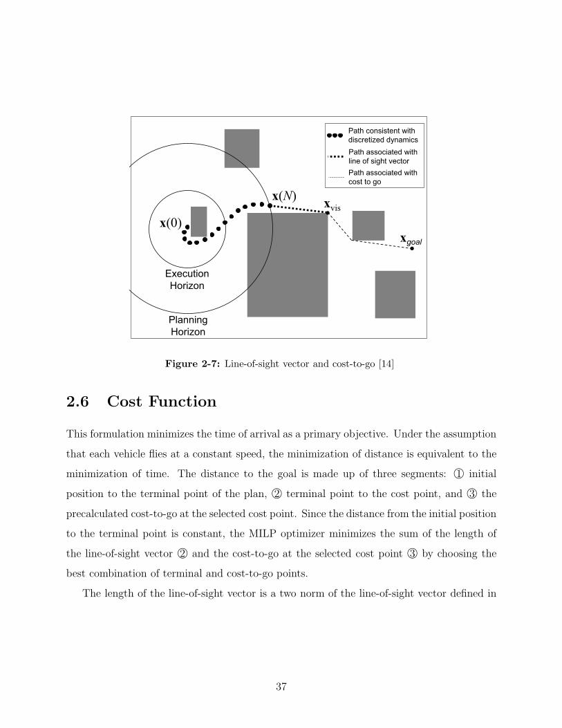
Figure 2-7: Line-of-sight vector and cost-to-go [14]

2.6 Cost Function

This formulation minimizes the time of arrival as a primary objective. Under the assumption

that each vehicle flies at a constant speed, the minimization of distance is equivalent to the

minimization of time. The distance to the goal is made up of three segments: 1© initial

position to the terminal point of the plan, 2© terminal point to the cost point, and 3© the

precalculated cost-to-go at the selected cost point. Since the distance from the initial position

to the terminal point is constant, the MILP optimizer minimizes the sum of the length of

the line-of-sight vector 2© and the cost-to-go at the selected cost point 3© by choosing the

best combination of terminal and cost-to-go points.

The length of the line-of-sight vector is a two norm of the line-of-sight vector defined in

37

Eq. 2.32. This is calculated in the MILP by minimizing an upper bound:

lj ≥ xLOS,j

yLOS,j

· ik (2.51)

ik =

cos

(2πk

nl

)

sin

(2πk

nl

) (2.52)

j = 1, . . . , nv, k = 1, . . . , nl

where nl is the number of unit vectors onto which the line-of-sight vector is projected and

lj gives an upper bound of the line-of-sight vector length for vehicle j. In this case, the

objective function J0 to be minimized is

J0 =nv∑j=1

(lj + cvis,j) (2.53)

where cvis,j is a cost-to-go at the cost point selected by the jth vehicle as defined in Eq. 2.29.

The time-step of arrival (TOA) for the jth vehicle is expressed as

TOAj =nt+1∑k=1

k barrival,kj, j = 1, . . . , nv (2.54)

Note that in Eq. 2.54, if k = nt+1 when barrival,kj = 1, then the jth vehicle will not reach the

target in the planning horizon, thereby resulting in a higher cost. Combined with Eq. 2.53,

the term TOA forms the objective function for the minimum time of arrival problem:

J1 =nv∑j=1

{α (vj∆t)TOAj + lj + cvis,j

}(2.55)

where vj∆t converts the discrete time-step (TOAj is an integer) into distance and α is a

large weighting factor that makes the first term dominant. With a small α, the vehicle tends

to minimize the cost-to-go, so that it arrives at the first goal at the terminal step in the

38

planning horizon. This is in contrast to the more desirable case of arriving at the first goal

before the terminal step, and then minimizing the cost-to-go to the next goal. Thus the

weight α must be larger than the number of steps required to go from the first goal to the

next goal.

Finally, the term Ja, containing two auxiliary terms, is added to the primary cost in

Eq. 2.55 to decrease the position and heading error at the target. The new cost to be

minimized is defined as

J = J1 + Ja (2.56)

where Ja =nv∑j=1

(βderr,j + γverr,j) (2.57)

Note that an overly large value of β results in “wobbling” near the target. The wobbling

occurs as the vehicle attempts to maneuver, such that on the same time-step when it enters

the target region, it arrives at the center of the target.

Also note that the equations involving the dynamics, constraints, and costs are not

dependent of the number of vehicles except for vehicle collision avoidance, and thus these

can be solved separately if vehicle collision avoidance is not an issue.

2.7 Example

A simple example is presented here to show the validity of this model. The model is de-

scribed in the modelling language AMPL, which calls CPLEX 7.1 as a MILP solver. The

computation is done on a Windows-based PC with CPU speed 2.2GHz (Pentium 4) and 512

MB RAM.

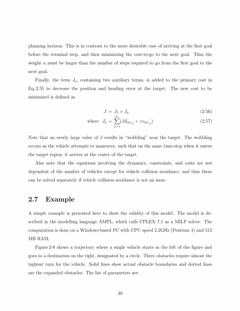
Figure 2-8 shows a trajectory where a single vehicle starts in the left of the figure and

goes to a destination on the right, designated by a circle. Three obstacles require almost the

tightest turn for the vehicle. Solid lines show actual obstacle boundaries and dotted lines

are the expanded obstacles. The list of parameters are:

39

−10 −8 −6 −4 −2 0 2 4 6 8 10 12−8

−6

−4

−2

0

2

4

6

8

x [m]

y [m

]

Figure 2-8: Trajectory with mini-mum speed constraints

−10 −8 −6 −4 −2 0 2 4 6 8 10 12−8

−6

−4

−2

0

2

4

6

8

x [m]

y [m

]

Figure 2-9: Trajectory without min-imum speed constraints

• v = 1• ∆t = 1.2• rmin = 2.8

• na = 20

• np = 5• ne = 1• nvmax = 20

• nvmin= 10

• nl = 36• M = 100

• Mv = 2vmin

Note that the optimal trajectory has waypoints on the obstacle boundaries. Figure 2-9

shows a trajectory without minimum speed constraints. Since it is still a minimum time

problem, there is not much difference in the trajectory. However, without minimum speed

constraints, the vehicle can slow down to make a tighter turn, making the effective minimum

turn radius smaller than that in Figure 2-8. Thus, the time-step of arrival in Figure 2-9 is

two steps less than that in Figure 2-8.

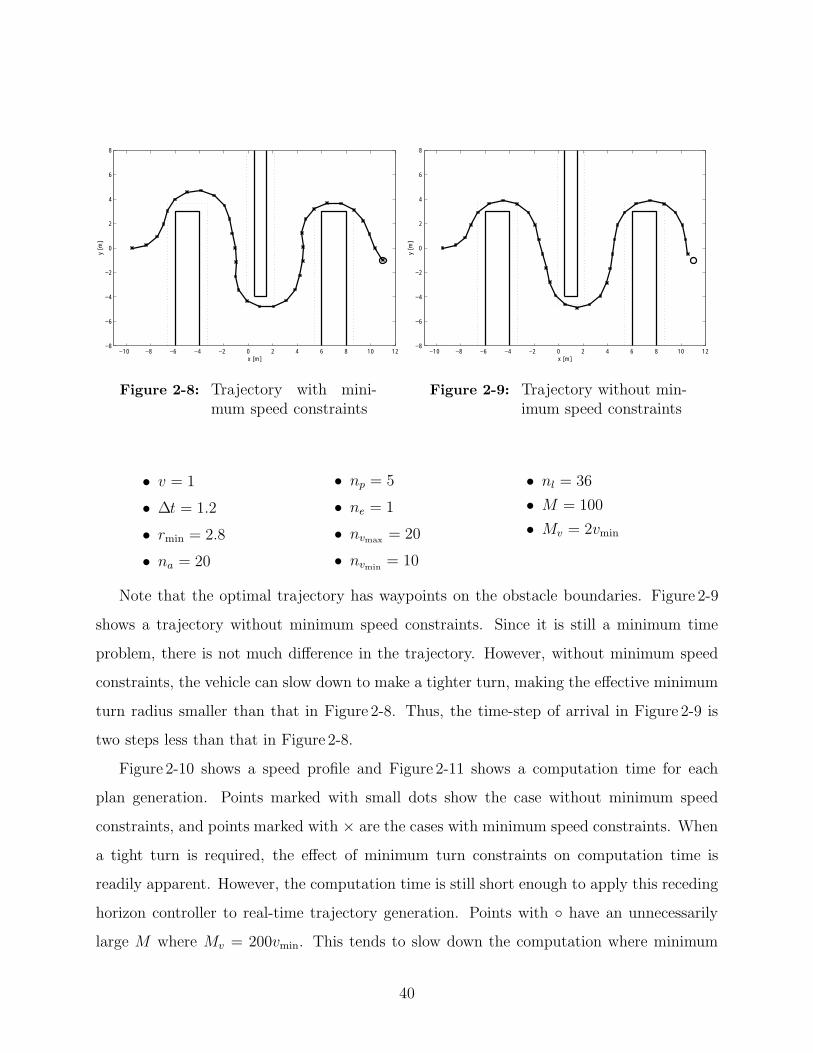
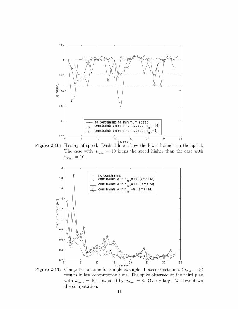
Figure 2-10 shows a speed profile and Figure 2-11 shows a computation time for each

plan generation. Points marked with small dots show the case without minimum speed

constraints, and points marked with × are the cases with minimum speed constraints. When

a tight turn is required, the effect of minimum turn constraints on computation time is

readily apparent. However, the computation time is still short enough to apply this receding

horizon controller to real-time trajectory generation. Points with ◦ have an unnecessarilylarge M where Mv = 200vmin. This tends to slow down the computation where minimum

40

0 5 10 15 20 25 30 350.75

0.8

0.85

0.9

0.95

1

1.05

time step

spee

d [m

/s]

no constraints on minimum speedconstraints on minimum speed (n

min=10)

constraints on minimum speed (nmin

=8)

Figure 2-10: History of speed. Dashed lines show the lower bounds on the speed.The case with nvmin

= 10 keeps the speed higher than the case withnvmin

= 10.

0 5 10 15 20 25 30 350.2

0.4

0.6

0.8

1

1.2

1.4

1.6

1.8

2

plan number

com

puta

tion

time

in [s

ec]

no constraintsconstraints with n

min=10, (small M)

constraints with nmin

=10, (large M)constraints with n

min=8, (small M)

Figure 2-11: Computation time for simple example. Looser constraints (nvmin= 8)

results in less computation time. The spike observed at the third planwith nvmin

= 10 is avoided by nvmin= 8. Overly large M slows down

the computation.41

turn constraints are active, which suggests the “big M” should be set as small as possible.

To compare with nvmin= 10, the resolution of the minimum speed constraints is reduced

to 8. Reducing nvminresults in much shorter computation time, as shown in Figure 2-11. It

allows the vehicle to slow down to 91% of the maximum speed1, whereas nvmin= 10 maintains

the speed to within 95% of the maximum speed. Thus in this example, a 40% reduction in

the computation time was obtained with only a 4% change in the minimum speed.

2.8 Conclusions

This chapter extended the previous work and posed the multi-vehicle multi-waypoint mini-

mum time-of-arrival trajectory generation problem in MILP form. The selection of the goal

is expressed in MILP form using binary variables that include other logical constraints such

as collision avoidance. The point mass model captures the essential features of the aircraft

dynamics such as speed and minimum turning radius constraints. The detailed analysis also

clarified the effect of the time discretization. The non-convex minimum speed constraints

have also been added to the problem to better capture the vehicle behavior in highly con-

strained environments. The effect on the computation time was also examined.

1The lower bound for the speed is obtained by finding the largest regular polygon that fits inside theregular polygon for the maximum speed constraints.

42

Chapter 3

Stable Receding Horizon Trajectory

Designer

This chapter presents a stable formulation of the receding horizon trajectory designer. The

“stability” of the trajectory designer is defined as a guaranteed arrival at the goal. In

the formulation presented in the previous chapter, a straight line approximation gives a

good cost estimate, but it can require too tight a turn because it does not account for the

vehicle dynamics. Replanning is usually able to find a dynamically feasible path around

the line segment path. However, in an extreme case described in Section 3.1, the large

heading discontinuities when the line segments join leads to an infeasible problem in the

detailed trajectory design phase. This situation is avoided by introducing three turning

circles per corner when building the cost map and extending the planning horizon sufficiently

far enough out beyond the execution horizon. Section 3.2 discusses the visibility graph that

constructs collision free paths in the world map. The modified Dijkstra’s algorithm presented

in Section 3.3 ensures there exists a feasible turn from one corner to another, and Section 3.4

discusses how to extract the necessary part of the cost map for the MILP optimization.

Finally, Section 3.5 reveals sufficient conditions required (based on the existence of a feasible

path) in the detailed trajectory design phase to prove the stability of the receding horizon

controller.

43

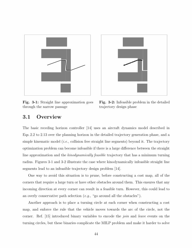
Fig. 3-1: Straight line approximation goesthrough the narrow passage

Fig. 3-2: Infeasible problem in the detailedtrajectory design phase

3.1 Overview

The basic receding horizon controller [14] uses an aircraft dynamics model described in

Eqs. 2.2 to 2.13 over the planning horizon in the detailed trajectory generation phase, and a

simple kinematic model (i.e., collision free straight line segments) beyond it. The trajectory

optimization problem can become infeasible if there is a large difference between the straight

line approximation and the kinodynamically feasible trajectory that has a minimum turning

radius. Figures 3-1 and 3-2 illustrate the case where kinodynamically infeasible straight line

segments lead to an infeasible trajectory design problem [14].

One way to avoid this situation is to prune, before constructing a cost map, all of the

corners that require a large turn or have other obstacles around them. This ensures that any

incoming direction at every corner can result in a feasible turn. However, this could lead to

an overly conservative path selection (e.g., “go around all the obstacles”).

Another approach is to place a turning circle at each corner when constructing a cost

map, and enforce the rule that the vehicle moves towards the arc of the circle, not the

corner. Ref. [15] introduced binary variables to encode the join and leave events on the

turning circles, but these binaries complicate the MILP problem and make it harder to solve

44

25 20 15 10 5 0 5 10 15 2015

10

5

0

5

10

15

A

B

Figure 3-3: Typical scenario populated with obstacles

while restricting the freedom of the trajectory designer to choose a path.

A new approach presented in this chapter ensures the existence of a kinodynamically

feasible turn at each corner by applying a modified Dijkstra’s algorithm when constructing

the cost map. When searching for the shortest path, this algorithm rejects a sequence of

nodes if the turning circles cannot be suitably placed (i.e., a kinodynamically infeasible

sequence). The generated tree of nodes gives the shortest distance from each node to the

goal along the straight lines in the regions where a feasible path is guaranteed to exist.

When optimizing the trajectory using RHC, the planning horizon is then extended beyond

the execution horizon such that while executing the plan, the vehicle will always stay in the

regions from which a feasible path to the goal exists.

3.2 Visibility Graph

This section extends the graph search algorithm from Ref. [13] which is used to generate a

coarse cost map for path planning in an obstacle field. Nodes for the graph are the obstacle

corners and the goal point. This is a good approximation, because with very fast turning

dynamics, the shortest path from one node to another would consist of the straight line

45

25 20 15 10 5 0 5 10 15 2015

10

5

0

5

10

15

A

B

Fig. 3-4: Visibility graph

−25 −20 −15 −10 −5 0 5 10 15 20−15

−10

−5

0

5

10

15

A

B

Fig. 3-5: Visibility graph after pruning

segments provided by the visibility graph. Figure 3-3 shows a typical scenario where many

obstacles reside between the vehicle location (marked as the ∗ middle left) and the goal(marked as a star in the upper right). Figure 3-4 shows all the collision free connections

between nodes. Two connected nodes in this figure are “visible” from each other.

Before running the Dijkstra’s algorithm to solve for the shortest path toward the single

source node, pruning some connections that will never be selected reduces the computation

time. In Figure 3-4, some connections are unnecessary since the vehicle will never follow

these paths. For example, the connection between node A and B can be pruned because a

vehicle going from A to B will collide with the obstacle to which node B is attached. More

generally, if a connected line segment is extended by ε at both ends, and either extended end

point is inside an obstacle, that connection can be removed. Figure 3-5 shows a visibility

graph after pruning – the number of connections has decreased from 367 to 232.

3.3 Modified Dijkstra’s Algorithm

This section extends the previous way of constructing the cost map, described in Section 3.2,

to ensure the existence of kinodynamically feasible paths around the straight line segments.

Proper placement of turning circles is critical in the less conservative estimate of the existence

of a feasible turn. An analytical way of placing collision free circles is introduced in Subsec-

46

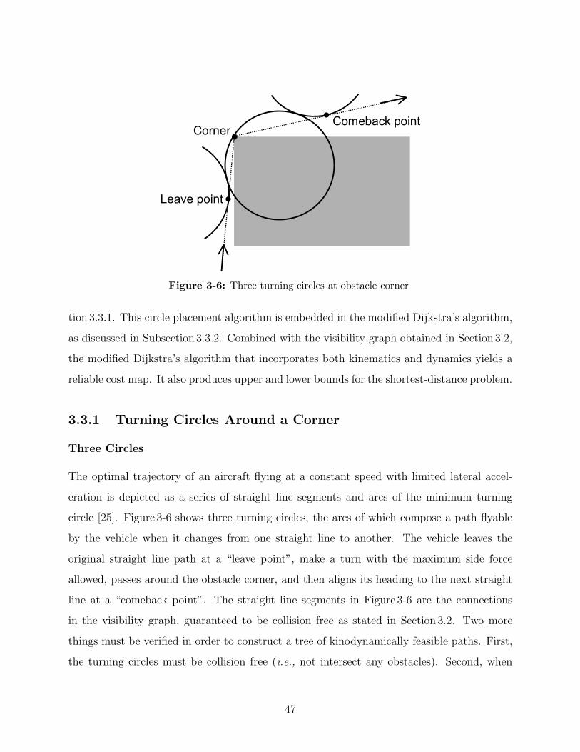
CornerComeback point

Leave point

Figure 3-6: Three turning circles at obstacle corner

tion 3.3.1. This circle placement algorithm is embedded in the modified Dijkstra’s algorithm,

as discussed in Subsection 3.3.2. Combined with the visibility graph obtained in Section 3.2,

the modified Dijkstra’s algorithm that incorporates both kinematics and dynamics yields a

reliable cost map. It also produces upper and lower bounds for the shortest-distance problem.

3.3.1 Turning Circles Around a Corner

Three Circles

The optimal trajectory of an aircraft flying at a constant speed with limited lateral accel-

eration is depicted as a series of straight line segments and arcs of the minimum turning

circle [25]. Figure 3-6 shows three turning circles, the arcs of which compose a path flyable

by the vehicle when it changes from one straight line to another. The vehicle leaves the

original straight line path at a “leave point”, make a turn with the maximum side force

allowed, passes around the obstacle corner, and then aligns its heading to the next straight

line at a “comeback point”. The straight line segments in Figure 3-6 are the connections

in the visibility graph, guaranteed to be collision free as stated in Section 3.2. Two more

things must be verified in order to construct a tree of kinodynamically feasible paths. First,

the turning circles must be collision free (i.e., not intersect any obstacles). Second, when

47

O θ1

rmin

rmin

O1

O0

L

C1

C0

l

H

0

0

x

y

P

O1

O1

x

yO0

O0

y=0

x=0

h

0

x

y

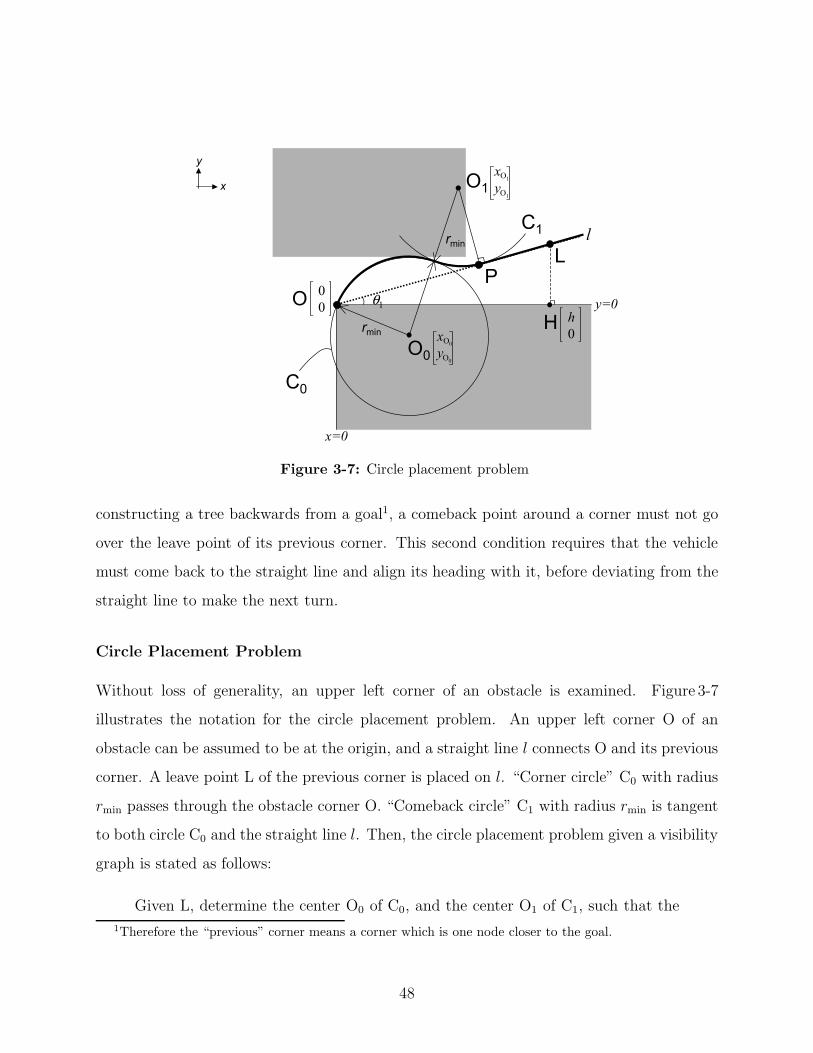
Figure 3-7: Circle placement problem

constructing a tree backwards from a goal1, a comeback point around a corner must not go

over the leave point of its previous corner. This second condition requires that the vehicle

must come back to the straight line and align its heading with it, before deviating from the

straight line to make the next turn.

Circle Placement Problem

Without loss of generality, an upper left corner of an obstacle is examined. Figure 3-7

illustrates the notation for the circle placement problem. An upper left corner O of an

obstacle can be assumed to be at the origin, and a straight line l connects O and its previous

corner. A leave point L of the previous corner is placed on l. “Corner circle” C0 with radius

rmin passes through the obstacle corner O. “Comeback circle” C1 with radius rmin is tangent

to both circle C0 and the straight line l. Then, the circle placement problem given a visibility

graph is stated as follows:

Given L, determine the center O0 of C0, and the center O1 of C1, such that the

1Therefore the “previous” corner means a corner which is one node closer to the goal.

48

O θ1

rmin

rmin

O1

O0

L

H

(a) Leave point is close to the corner

Oθ1

rmin

rmin

O1

O0

B L

A H

(b) Leave point is far from the corner

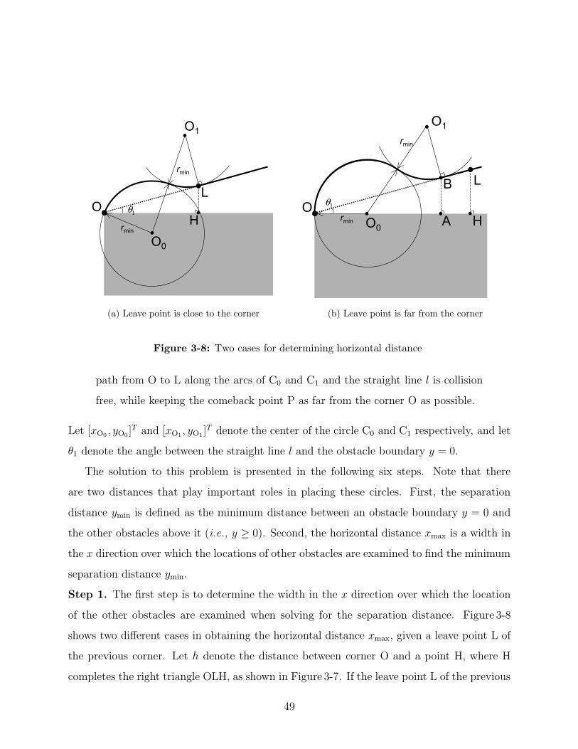
Figure 3-8: Two cases for determining horizontal distance

path from O to L along the arcs of C0 and C1 and the straight line l is collision

free, while keeping the comeback point P as far from the corner O as possible.

Let [xO0 , yO0]T and [xO1 , yO1]

T denote the center of the circle C0 and C1 respectively, and let

θ1 denote the angle between the straight line l and the obstacle boundary y = 0.

The solution to this problem is presented in the following six steps. Note that there

are two distances that play important roles in placing these circles. First, the separation

distance ymin is defined as the minimum distance between an obstacle boundary y = 0 and

the other obstacles above it (i.e., y ≥ 0). Second, the horizontal distance xmax is a width in

the x direction over which the locations of other obstacles are examined to find the minimum

separation distance ymin.

Step 1. The first step is to determine the width in the x direction over which the location

of the other obstacles are examined when solving for the separation distance. Figure 3-8

shows two different cases in obtaining the horizontal distance xmax, given a leave point L of

the previous corner. Let h denote the distance between corner O and a point H, where H

completes the right triangle OLH, as shown in Figure 3-7. If the leave point L of the previous

49

corner is “close” to the corner, as in Figure 3-8(a), only the region OH needs to be examined

to find the minimum separation distance. If it is “far”, as in Figure 3-8(b), the center of the

corner circle is set temporarily at [0, rmin]T so that the comeback point P associated with

corner O gets as close as possible to the leave point L of the previous corner. Note that

in Figure 3-8(b), if the thick line turns out to be collision free, any incoming direction to

the corner O (from y ≤ 0) is able to produce a kinodynamically feasible turn that joins the

straight line before reaching the leave point L. The “close” case and the “far” case are held

together to define the horizontal distance xmax as follows.

xmax = min(OH,OA)

= min

h, rmin(1 +

√3 + 2 tan2 θ1 − 2 tan θ1

√1 + tan2 θ1)

1 + tan2 θ1

(3.1)

where the second term is the length of OA in Figure 3-8(b) and is analytically obtained2.

The comeback point P has not yet been determined.

Step 2. The minimum separation distance ymin is obtained by examining obstacle corners

and lines in the region{(x, y)

∣∣∣ 0 ≤ x ≤ xmax, x tan θ1 ≤ y}, so that there are no obstacles

in the region{(x, y)

∣∣∣ 0 ≤ x ≤ xmax, x tan θ1 ≤ y ≤ ymin

}. It guarantees that if two arcs of

C0 and C1 stay in the region{(x, y)

∣∣∣ 0 ≤ x ≤ xmax, x tan θ1 ≤ y ≤ ymin

}, then there exists a

kinodynamically feasible path from O to L, which is a connection of the two arcs of C0 and

C1 and the straight line l.

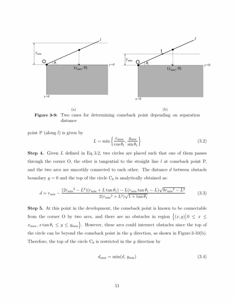
Step 3. When determining the comeback point P, two cases must be considered, as shown

in Figure 3-9, depending on the separation distance ymin. If the separation distance is large

enough as in Figure 3-9(a), the leave point L in Figure 3-8(a) or point B in Figure 3-8(b)

becomes the comeback point P associated with the corner O. If the separation distance is

too small, as in Figure 3-9(b), the intersection I of two lines y = ymin and straight line

l becomes the comeback point P since the region{(x, y)

∣∣∣ y > ymin, y > x tan θ1}is not

guaranteed to be collision free. Therefore, the distance L between corner O and comeback

2This result was analytically obtained using Mathematica.

50

O θ1

ymin

(xmax, 0)

l

y=0

x=0

(a)

O θ1

ymin

(xmax, 0)

I

l

y=0

x=0

(b)

Figure 3-9: Two cases for determining comeback point depending on separationdistance

point P (along l) is given by

L = min{xmax

cos θ1,ymin

sin θ1

}(3.2)

Step 4. Given L defined in Eq. 3.2, two circles are placed such that one of them passes

through the corner O, the other is tangential to the straight line l at comeback point P,

and the two arcs are smoothly connected to each other. The distance d between obstacle

boundary y = 0 and the top of the circle C0 is analytically obtained as:

d = rmin − (2rmin2 − L2)(rmin + L tan θ1)− L(rmin tan θ1 − L)

√8rmin

2 − L2

2(rmin2 + L2)

√1 + tan θ1

(3.3)

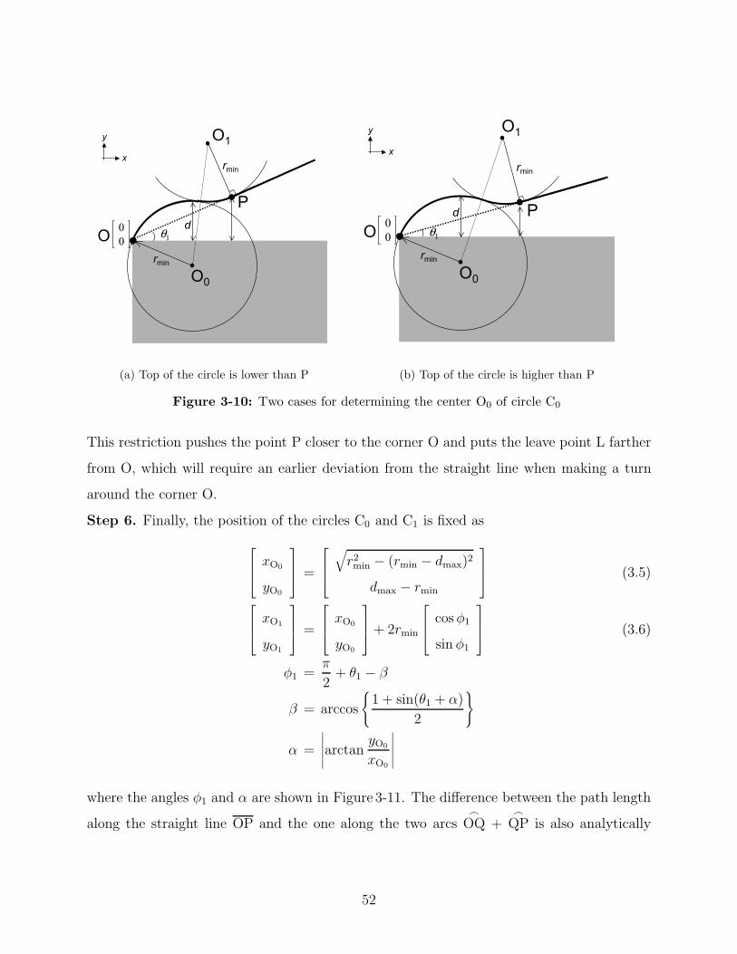
Step 5. At this point in the development, the comeback point is known to be connectable

from the corner O by two arcs, and there are no obstacles in region{(x, y)

∣∣∣ 0 ≤ x ≤xmax, x tan θ1 ≤ y ≤ ymax

}. However, these arcs could intersect obstacles since the top of

the circle can be beyond the comeback point in the y direction, as shown in Figure 3-10(b).

Therefore, the top of the circle C0 is restricted in the y direction by

dmax = min(d, ymin) (3.4)

51

θ1

rmin

rmin

O1

O0

P

d

O0

0

x

y

(a) Top of the circle is lower than P

θ1

rmin

rmin

O1

O0

Pd

O0

0

x

y

(b) Top of the circle is higher than P

Figure 3-10: Two cases for determining the center O0 of circle C0

This restriction pushes the point P closer to the corner O and puts the leave point L farther

from O, which will require an earlier deviation from the straight line when making a turn

around the corner O.

Step 6. Finally, the position of the circles C0 and C1 is fixed as

xO0

yO0

=

√r2min − (rmin − dmax)2

dmax − rmin

(3.5)

xO1

yO1

=

xO0

yO0

+ 2rmin

cosφ1

sin φ1

(3.6)

φ1 =π

2+ θ1 − β

β = arccos

{1 + sin(θ1 + α)

2

}

α =

∣∣∣∣∣arctan yO0

xO0

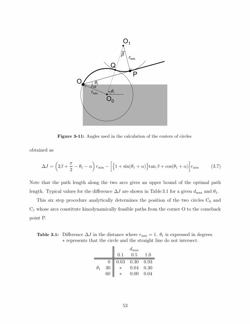
∣∣∣∣∣where the angles φ1 and α are shown in Figure 3-11. The difference between the path length

along the straight line OP and the one along the two arcs�

OQ +�

QP is also analytically

52

O θ1

rmin

rmin

O1

O0

P

αφ1

Q

β

Figure 3-11: Angles used in the calculation of the centers of circles

obtained as

∆J =(2β +

π

2− θ1 − α

)rmin −

[{1 + sin(θ1 + α)

}tan β + cos(θ1 + α)

]rmin (3.7)

Note that the path length along the two arcs gives an upper bound of the optimal path

length. Typical values for the difference ∆J are shown in Table 3.1 for a given dmax and θ1.

This six step procedure analytically determines the position of the two circles C0 and

C1 whose arcs constitute kinodynamically feasible paths from the corner O to the comeback

point P.

Table 3.1: Difference ∆J in the distance where rmin = 1. θ1 is expressed in degrees.∗ represents that the circle and the straight line do not intersect.

dmax

0.1 0.5 1.0

0 0.03 0.30 0.93θ1 30 ∗ 0.04 0.30

60 ∗ 0.00 0.04

53

O θ1

rmin

rmin

O1

O0

P

rmin

LO2

α

θ2

l

m

φ1φ2

0

0

x

y

(a) Tight incoming direction

θ1

rmin

O1

O0

P

θ2

α

l

m

φ1rmin

O0

0

x

y

(b) No need to place leave circle

Figure 3-12: Two cases for determining the center O2 of circle C2

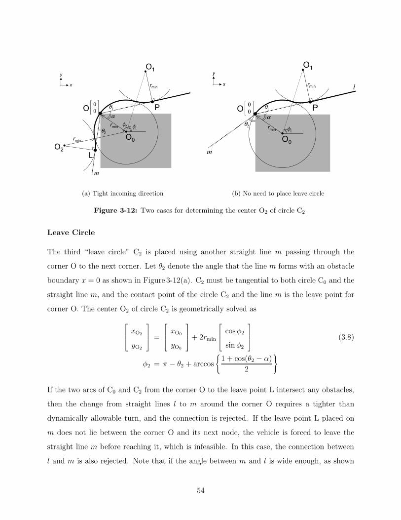
Leave Circle

The third “leave circle” C2 is placed using another straight line m passing through the

corner O to the next corner. Let θ2 denote the angle that the line m forms with an obstacle

boundary x = 0 as shown in Figure 3-12(a). C2 must be tangential to both circle C0 and the

straight line m, and the contact point of the circle C2 and the line m is the leave point for

corner O. The center O2 of circle C2 is geometrically solved as

xO2

yO2

=

xO0

yO0

+ 2rmin

cosφ2

sin φ2

(3.8)

φ2 = π − θ2 + arccos{1 + cos(θ2 − α)

2

}

If the two arcs of C0 and C2 from the corner O to the leave point L intersect any obstacles,

then the change from straight lines l to m around the corner O requires a tighter than

dynamically allowable turn, and the connection is rejected. If the leave point L placed on

m does not lie between the corner O and its next node, the vehicle is forced to leave the

straight line m before reaching it, which is infeasible. In this case, the connection between

l and m is also rejected. Note that if the angle between m and l is wide enough, as shown

54

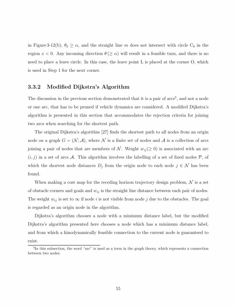
in Figure 3-12(b), θ2 ≥ α, and the straight line m does not intersect with circle C0 in the

region x < 0. Any incoming direction θ (≥ α) will result in a feasible turn, and there is no

need to place a leave circle. In this case, the leave point L is placed at the corner O, which

is used in Step 1 for the next corner.

3.3.2 Modified Dijkstra’s Algorithm

The discussion in the previous section demonstrated that it is a pair of arcs3, and not a node

or one arc, that has to be pruned if vehicle dynamics are considered. A modified Dijkstra’s

algorithm is presented in this section that accommodates the rejection criteria for joining

two arcs when searching for the shortest path.

The original Dijkstra’s algorithm [27] finds the shortest path to all nodes from an origin

node on a graph G = (N ;A), where N is a finite set of nodes and A is a collection of arcs

joining a pair of nodes that are members of N . Weight wij(≥ 0) is associated with an arc

(i, j) in a set of arcs A. This algorithm involves the labelling of a set of fixed nodes P, ofwhich the shortest node distances Dj from the origin node to each node j ∈ N has been

found.

When making a cost map for the receding horizon trajectory design problem, N is a set

of obstacle corners and goals and wij is the straight line distance between each pair of nodes.

The weight wij is set to∞ if node i is not visible from node j due to the obstacles. The goal

is regarded as an origin node in the algorithm.

Dijkstra’s algorithm chooses a node with a minimum distance label, but the modified

Dijkstra’s algorithm presented here chooses a node which has a minimum distance label,

and from which a kinodynamically feasible connection to the current node is guaranteed to

exist.

3In this subsection, the word “arc” is used as a term in the graph theory, which represents a connectionbetween two nodes.

55

Algorithm Overview

The index of the goal node can be set to be 1. The modified Dijkstra’s algorithm then

consists of the following procedure:

1. Set current node i = 1, and initialize:

P = {1}

Dj =

0 (j = 1)

w1j (j �= 1)(3.9)

2. Place the leave point for the goal on the goal.

3. Set node i as the successor of each node j. A successor node is the next node on the

path toward the goal.

4. Find the next closest node from the set of unfixed nodes4, and set it as a new current

node i:

i := argminj �∈P

Dj (3.10)

5. Place the two turning circles C0 and C1 around node i.

6. Fix node i, and update the set P of fixed nodes:

P := P ∪ {i} (3.11)

7. If all nodes in N are also in the set P of fixed nodes, terminate.

8. For all the nodes that are unfixed and visible from the current node i, i.e., for each

{ j | j �∈ P, wij �=∞}:

(a) Place a leave circle around i, and put a leave point for i on a straight line con-

necting i and j.

4“Unfixed” means that the shortest path to the goal has not been found.

56

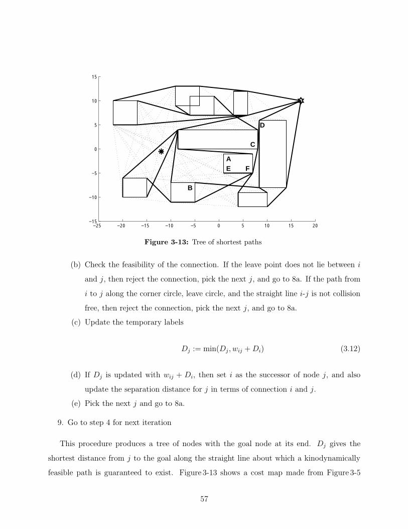
−25 −20 −15 −10 −5 0 5 10 15 20−15

−10

−5

0

5

10

15

A

B

C

D

E F

Figure 3-13: Tree of shortest paths

(b) Check the feasibility of the connection. If the leave point does not lie between i

and j, then reject the connection, pick the next j, and go to 8a. If the path from

i to j along the corner circle, leave circle, and the straight line i-j is not collision

free, then reject the connection, pick the next j, and go to 8a.

(c) Update the temporary labels

Dj := min(Dj , wij +Di) (3.12)

(d) If Dj is updated with wij + Di, then set i as the successor of node j, and also

update the separation distance for j in terms of connection i and j.

(e) Pick the next j and go to 8a.

9. Go to step 4 for next iteration

This procedure produces a tree of nodes with the goal node at its end. Dj gives the

shortest distance from j to the goal along the straight line about which a kinodynamically

feasible path is guaranteed to exist. Figure 3-13 shows a cost map made from Figure 3-5

57

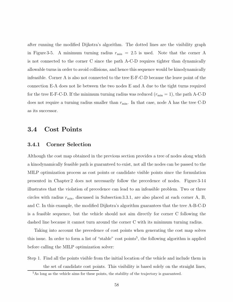
after running the modified Dijkstra’s algorithm. The dotted lines are the visibility graph

in Figure 3-5. A minimum turning radius rmin = 2.5 is used. Note that the corner A

is not connected to the corner C since the path A-C-D requires tighter than dynamically

allowable turns in order to avoid collisions, and hence this sequence would be kinodynamically

infeasible. Corner A is also not connected to the tree E-F-C-D because the leave point of the

connection E-A does not lie between the two nodes E and A due to the tight turns required

for the tree E-F-C-D. If the minimum turning radius was reduced (rmin = 1), the path A-C-D

does not require a turning radius smaller than rmin. In that case, node A has the tree C-D

as its successor.

3.4 Cost Points

3.4.1 Corner Selection

Although the cost map obtained in the previous section provides a tree of nodes along which

a kinodynamically feasible path is guaranteed to exist, not all the nodes can be passed to the

MILP optimization process as cost points or candidate visible points since the formulation

presented in Chapter 2 does not necessarily follow the precedence of nodes. Figure 3-14

illustrates that the violation of precedence can lead to an infeasible problem. Two or three

circles with radius rmin, discussed in Subsection 3.3.1, are also placed at each corner A, B,

and C. In this example, the modified Dijkstra’s algorithm guarantees that the tree A-B-C-D

is a feasible sequence, but the vehicle should not aim directly for corner C following the

dashed line because it cannot turn around the corner C with its minimum turning radius.

Taking into account the precedence of cost points when generating the cost map solves

this issue. In order to form a list of “stable” cost points5, the following algorithm is applied

before calling the MILP optimization solver:

Step 1. Find all the points visible from the initial location of the vehicle and include them in

the set of candidate cost points. This visibility is based solely on the straight lines,5As long as the vehicle aims for these points, the stability of the trajectory is guaranteed.

58

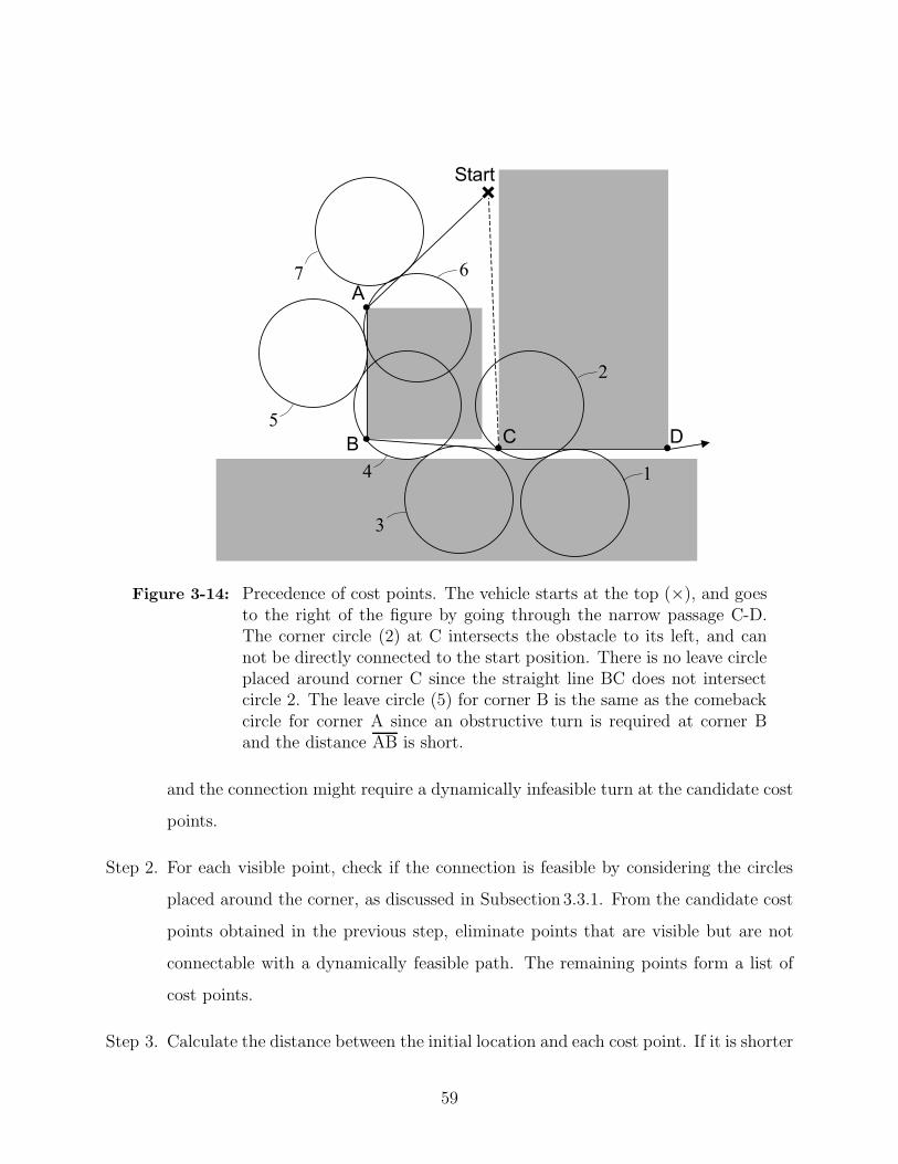
A

B C D

Start

1

2

3

4

5

7 6

Figure 3-14: Precedence of cost points. The vehicle starts at the top (×), and goesto the right of the figure by going through the narrow passage C-D.The corner circle (2) at C intersects the obstacle to its left, and cannot be directly connected to the start position. There is no leave circleplaced around corner C since the straight line BC does not intersectcircle 2. The leave circle (5) for corner B is the same as the comebackcircle for corner A since an obstructive turn is required at corner Band the distance AB is short.

and the connection might require a dynamically infeasible turn at the candidate cost

points.

Step 2. For each visible point, check if the connection is feasible by considering the circles

placed around the corner, as discussed in Subsection 3.3.1. From the candidate cost

points obtained in the previous step, eliminate points that are visible but are not

connectable with a dynamically feasible path. The remaining points form a list of

cost points.

Step 3. Calculate the distance between the initial location and each cost point. If it is shorter

59

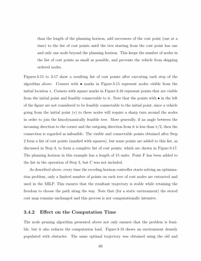
than the length of the planning horizon, add successors of the cost point (one at a

time) to the list of cost points until the tree starting from the cost point has one

and only one node beyond the planning horizon. This keeps the number of nodes in

the list of cost points as small as possible, and prevents the vehicle from skipping

ordered nodes.

Figures 3-15 to 3-17 show a resulting list of cost points after executing each step of the

algorithm above. Corners with • marks in Figure 3-15 represent nodes visible from the

initial location ∗. Corners with square marks in Figure 3-16 represent points that are visiblefrom the initial point and feasibly connectable to it. Note that the points with • in the leftof the figure are not considered to be feasibly connectable to the initial point, since a vehicle

going from the initial point (∗) to these nodes will require a sharp turn around the nodesin order to join the kinodynamically feasible tree. More generally, if an angle between the

incoming direction to the corner and the outgoing direction from it is less than π/2, then the

connection is regarded as infeasible. The visible and connectable points obtained after Step

2 form a list of cost points (marked with squares), but some points are added to this list, as

discussed in Step 3, to form a complete list of cost points, which are shown in Figure 3-17.

The planning horizon in this example has a length of 15 units. Point F has been added to

the list in the operation of Step 3, but C was not included.

As described above, every time the receding horizon controller starts solving an optimiza-

tion problem, only a limited number of points on each tree of cost nodes are extracted and

used in the MILP. This ensures that the resultant trajectory is stable while retaining the

freedom to choose the path along the way. Note that (for a static environment) the stored

cost map remains unchanged and this process is not computationally intensive.

3.4.2 Effect on the Computation Time

The node pruning algorithm presented above not only ensures that the problem is feasi-

ble, but it also reduces the computation load. Figure 3-18 shows an environment densely

populated with obstacles. The same optimal trajectory was obtained using the old and

60

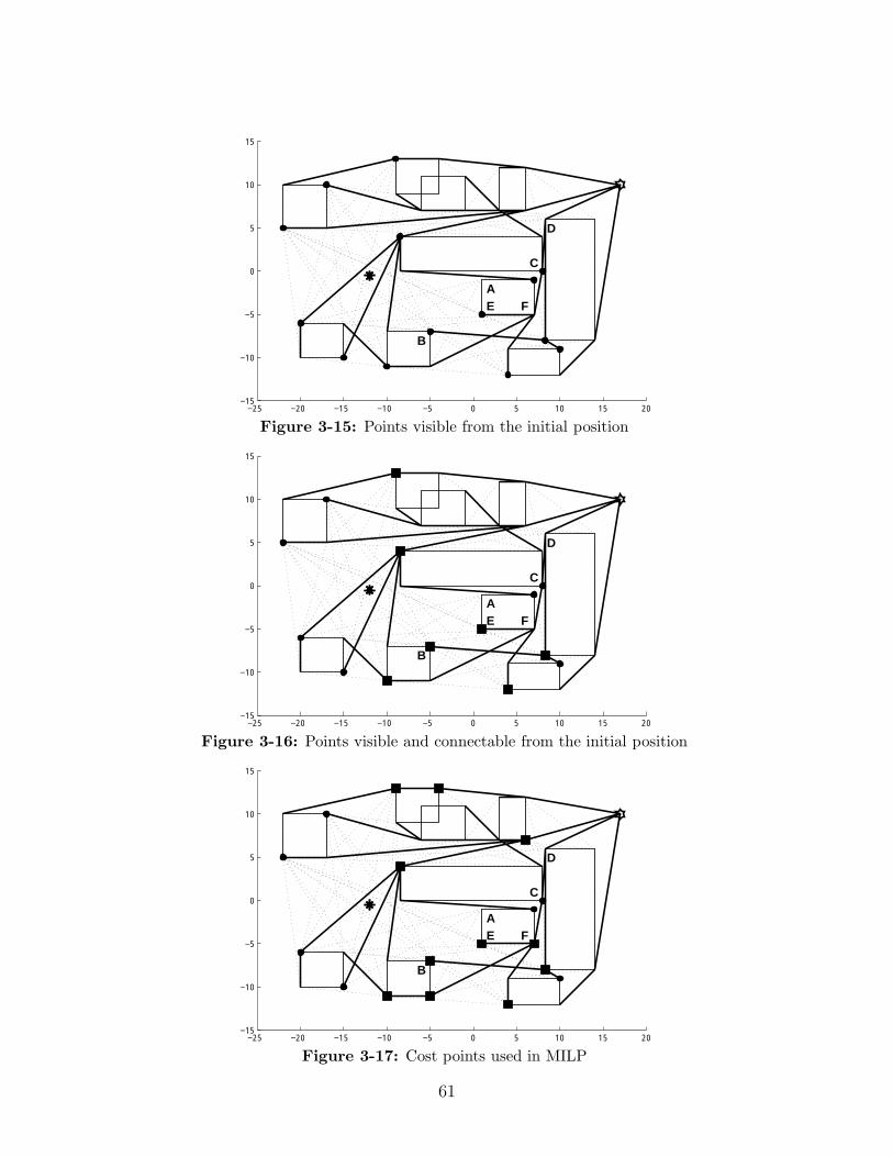
−25 −20 −15 −10 −5 0 5 10 15 20−15

−10

−5

0

5

10

15

A

B

C

D

E F

Figure 3-15: Points visible from the initial position

−25 −20 −15 −10 −5 0 5 10 15 20−15

−10

−5

0

5

10

15

A

B

C

D

E F

Figure 3-16: Points visible and connectable from the initial position

−25 −20 −15 −10 −5 0 5 10 15 20−15

−10

−5

0

5

10

15

A

B

C

D

E F

Figure 3-17: Cost points used in MILP

61

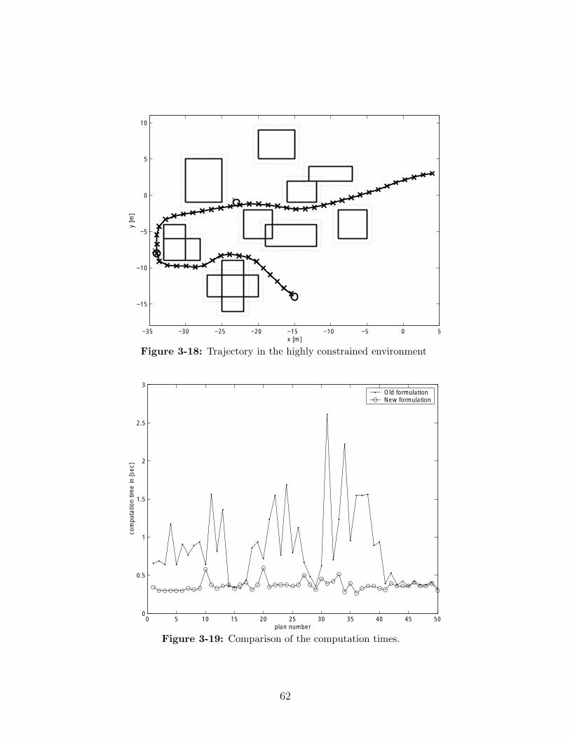
−35 −30 −25 −20 −15 −10 −5 0 5

−15

−10

−5

0

5

10

x [m]

y [m

]

1

2

3

Figure 3-18: Trajectory in the highly constrained environment

0 5 10 15 20 25 30 35 40 45 500

0.5

1

1.5

2

2.5

3

plan number

com

puta

tion

time

in [s

ec]

Old formulationNew formulation

Figure 3-19: Comparison of the computation times.

62

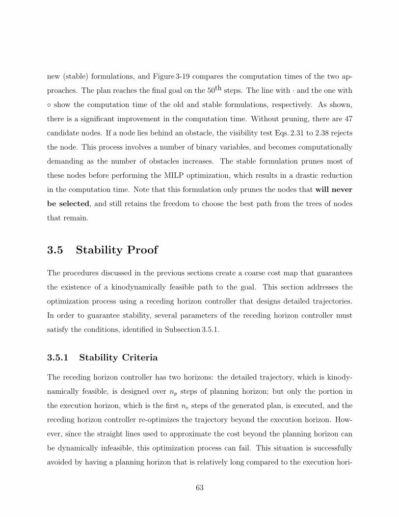
new (stable) formulations, and Figure 3-19 compares the computation times of the two ap-

proaches. The plan reaches the final goal on the 50th steps. The line with · and the one with◦ show the computation time of the old and stable formulations, respectively. As shown,

there is a significant improvement in the computation time. Without pruning, there are 47

candidate nodes. If a node lies behind an obstacle, the visibility test Eqs. 2.31 to 2.38 rejects

the node. This process involves a number of binary variables, and becomes computationally

demanding as the number of obstacles increases. The stable formulation prunes most of

these nodes before performing the MILP optimization, which results in a drastic reduction

in the computation time. Note that this formulation only prunes the nodes that will never

be selected, and still retains the freedom to choose the best path from the trees of nodes

that remain.

3.5 Stability Proof

The procedures discussed in the previous sections create a coarse cost map that guarantees

the existence of a kinodynamically feasible path to the goal. This section addresses the

optimization process using a receding horizon controller that designs detailed trajectories.

In order to guarantee stability, several parameters of the receding horizon controller must

satisfy the conditions, identified in Subsection 3.5.1.

3.5.1 Stability Criteria

The receding horizon controller has two horizons: the detailed trajectory, which is kinody-

namically feasible, is designed over np steps of planning horizon; but only the portion in

the execution horizon, which is the first ne steps of the generated plan, is executed, and the

receding horizon controller re-optimizes the trajectory beyond the execution horizon. How-

ever, since the straight lines used to approximate the cost beyond the planning horizon can

be dynamically infeasible, this optimization process can fail. This situation is successfully

avoided by having a planning horizon that is relatively long compared to the execution hori-

63

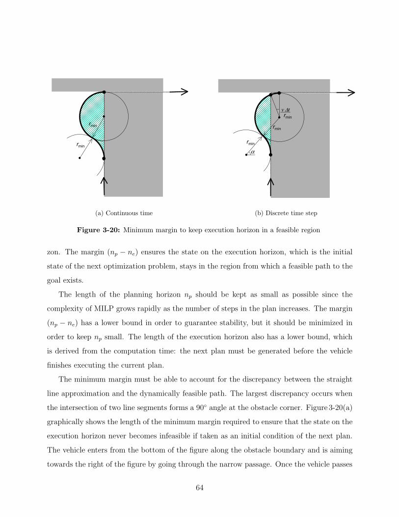
rmin

rmin

(a) Continuous time

rmin

rmin

v ∆trmin

α

(b) Discrete time step

Figure 3-20: Minimum margin to keep execution horizon in a feasible region

zon. The margin (np − ne) ensures the state on the execution horizon, which is the initialstate of the next optimization problem, stays in the region from which a feasible path to the

goal exists.

The length of the planning horizon np should be kept as small as possible since the

complexity of MILP grows rapidly as the number of steps in the plan increases. The margin

(np − ne) has a lower bound in order to guarantee stability, but it should be minimized inorder to keep np small. The length of the execution horizon also has a lower bound, which

is derived from the computation time: the next plan must be generated before the vehicle

finishes executing the current plan.

The minimum margin must be able to account for the discrepancy between the straight

line approximation and the dynamically feasible path. The largest discrepancy occurs when

the intersection of two line segments forms a 90◦ angle at the obstacle corner. Figure 3-20(a)

graphically shows the length of the minimum margin required to ensure that the state on the

execution horizon never becomes infeasible if taken as an initial condition of the next plan.

The vehicle enters from the bottom of the figure along the obstacle boundary and is aiming

towards the right of the figure by going through the narrow passage. Once the vehicle passes

64

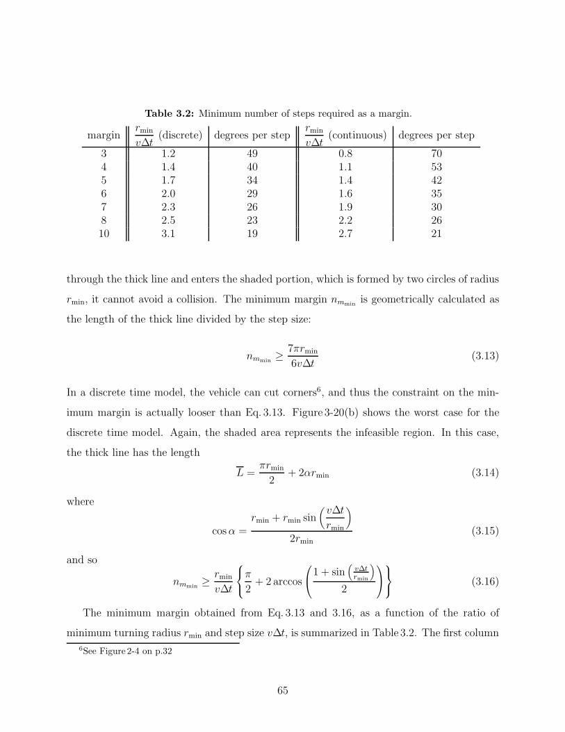
Table 3.2: Minimum number of steps required as a margin.

marginrmin

v∆t(discrete) degrees per step

rmin

v∆t(continuous) degrees per step

3 1.2 49 0.8 704 1.4 40 1.1 535 1.7 34 1.4 426 2.0 29 1.6 357 2.3 26 1.9 308 2.5 23 2.2 2610 3.1 19 2.7 21

through the thick line and enters the shaded portion, which is formed by two circles of radius

rmin, it cannot avoid a collision. The minimum margin nmminis geometrically calculated as

the length of the thick line divided by the step size:

nmmin≥ 7πrmin

6v∆t(3.13)

In a discrete time model, the vehicle can cut corners6, and thus the constraint on the min-

imum margin is actually looser than Eq. 3.13. Figure 3-20(b) shows the worst case for the

discrete time model. Again, the shaded area represents the infeasible region. In this case,

the thick line has the length

L =πrmin

2+ 2αrmin (3.14)

where

cosα =rmin + rmin sin

(v∆t

rmin

)2rmin

(3.15)

and so

nmmin≥ rmin

v∆t

π2 + 2 arccos

1 + sin

(v∆trmin

)2

(3.16)

The minimum margin obtained from Eq. 3.13 and 3.16, as a function of the ratio of

minimum turning radius rmin and step size v∆t, is summarized in Table 3.2. The first column

6See Figure 2-4 on p.32

65

shows the minimum number of steps required as a margin given the ratio rmin/(v∆t). If the

ratio is in between the two numbers, the larger value must be used to ensure stability when

selecting the minimum margin from this table. With the same step size v∆ t, a larger

minimum turning radius requires a larger margin7 since the vehicle is less agile. With the

same minimum turning radius, a smaller v∆t requires a larger margin since the waypoints

on the trajectory are more detailed.

The third and fifth columns give the central angle per step for a given rmin/(v∆t) when

turning along the circle with a minimum turning radius. As the angle per step decreases,

i.e., the vehicle follows the turning circle with more detailed waypoints, a larger number of

steps is required as a margin. Note that a larger margin causes longer computation time;

this represents a trade-off between the computation load and the resolution of the trajectory.

Simulation Result

The simulation result in Figure 3-21 demonstrates the stability of the receding horizon con-

troller. Original obstacles are depicted by solid lines, while dashed lines show obstacle

boundaries expanded to account for the discrete time model8. Solid lines with bullets show

the detailed trajectory, and dotted lines with bullets show the waypoints of the previous

plan. The vehicle starts at the bottom of the figure and goes to the upper right by passing

through the narrow passage. From (a) to (f), the vehicle executes one step at a time. A

circle introduced in Figure 3-20(b) is placed to show the infeasible region. The following

parameters are used in this simulation.

• np = 11• ne = 1• rmin = 3.1

• v∆t = 17“Large” in the sense that the number of steps is large.8See Figure 2-4 for obstacle enlargement.

66

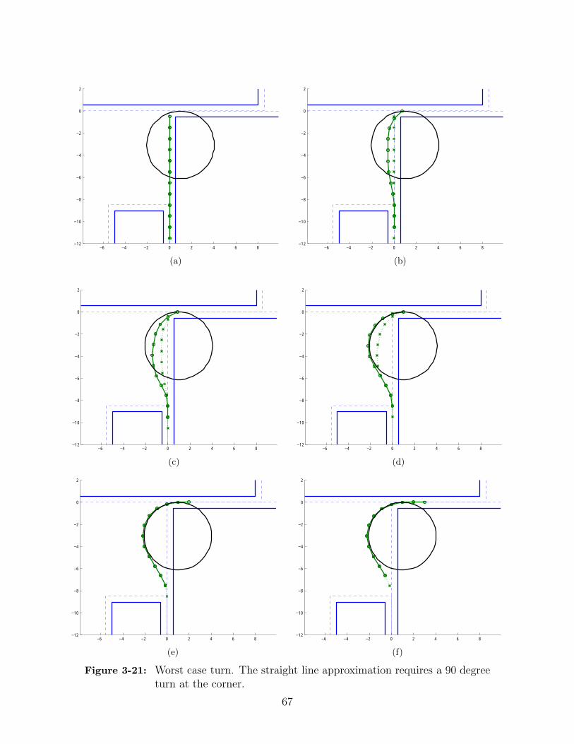
−6 −4 −2 0 2 4 6 8−12

−10

−8

−6

−4

−2

0

2

(a)

−6 −4 −2 0 2 4 6 8−12

−10

−8

−6

−4

−2

0

2

(b)

−6 −4 −2 0 2 4 6 8−12

−10

−8

−6

−4

−2

0

2

(c)

−6 −4 −2 0 2 4 6 8−12

−10

−8

−6

−4

−2

0

2

(d)

−6 −4 −2 0 2 4 6 8−12

−10

−8

−6

−4

−2

0

2

(e)

−6 −4 −2 0 2 4 6 8−12

−10

−8

−6

−4

−2

0

2

(f)

Figure 3-21: Worst case turn. The straight line approximation requires a 90 degreeturn at the corner.

67

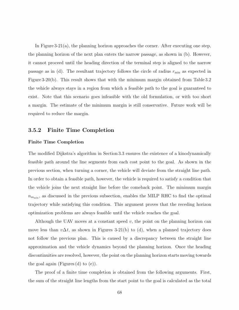
In Figure 3-21(a), the planning horizon approaches the corner. After executing one step,

the planning horizon of the next plan enters the narrow passage, as shown in (b). However,

it cannot proceed until the heading direction of the terminal step is aligned to the narrow

passage as in (d). The resultant trajectory follows the circle of radius rmin as expected in

Figure 3-20(b). This result shows that with the minimum margin obtained from Table 3.2

the vehicle always stays in a region from which a feasible path to the goal is guaranteed to

exist. Note that this scenario goes infeasible with the old formulation, or with too short

a margin. The estimate of the minimum margin is still conservative. Future work will be

required to reduce the margin.

3.5.2 Finite Time Completion

Finite Time Completion

The modified Dijkstra’s algorithm in Section 3.3 ensures the existence of a kinodynamically

feasible path around the line segments from each cost point to the goal. As shown in the

previous section, when turning a corner, the vehicle will deviate from the straight line path.

In order to obtain a feasible path, however, the vehicle is required to satisfy a condition that

the vehicle joins the next straight line before the comeback point. The minimum margin

nmmin, as discussed in the previous subsection, enables the MILP RHC to find the optimal

trajectory while satisfying this condition. This argument proves that the receding horizon

optimization problems are always feasible until the vehicle reaches the goal.

Although the UAV moves at a constant speed v, the point on the planning horizon can

move less than v∆t, as shown in Figures 3-21(b) to (d), when a planned trajectory does

not follow the previous plan. This is caused by a discrepancy between the straight line

approximation and the vehicle dynamics beyond the planning horizon. Once the heading

discontinuities are resolved, however, the point on the planning horizon starts moving towards

the goal again (Figures (d) to (e)).

The proof of a finite time completion is obtained from the following arguments. First,

the sum of the straight line lengths from the start point to the goal is calculated as the total

68

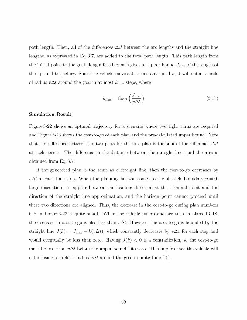
path length. Then, all of the differences ∆J between the arc lengths and the straight line

lengths, as expressed in Eq. 3.7, are added to the total path length. This path length from

the initial point to the goal along a feasible path gives an upper bound Jmax of the length of

the optimal trajectory. Since the vehicle moves at a constant speed v, it will enter a circle

of radius v∆t around the goal in at most kmax steps, where

kmax = floor(Jmax

v∆t

)(3.17)

Simulation Result

Figure 3-22 shows an optimal trajectory for a scenario where two tight turns are required

and Figure 3-23 shows the cost-to-go of each plan and the pre-calculated upper bound. Note

that the difference between the two plots for the first plan is the sum of the difference ∆J

at each corner. The difference in the distance between the straight lines and the arcs is

obtained from Eq. 3.7.

If the generated plan is the same as a straight line, then the cost-to-go decreases by

v∆t at each time step. When the planning horizon comes to the obstacle boundary y = 0,

large discontinuities appear between the heading direction at the terminal point and the

direction of the straight line approximation, and the horizon point cannot proceed until

these two directions are aligned. Thus, the decrease in the cost-to-go during plan numbers

6–8 in Figure 3-23 is quite small. When the vehicle makes another turn in plans 16–18,

the decrease in cost-to-go is also less than v∆t. However, the cost-to-go is bounded by the

straight line J(k) = Jmax − k(v∆t), which constantly decreases by v∆t for each step andwould eventually be less than zero. Having J(k) < 0 is a contradiction, so the cost-to-go

must be less than v∆t before the upper bound hits zero. This implies that the vehicle will

enter inside a circle of radius v∆t around the goal in finite time [15].

69

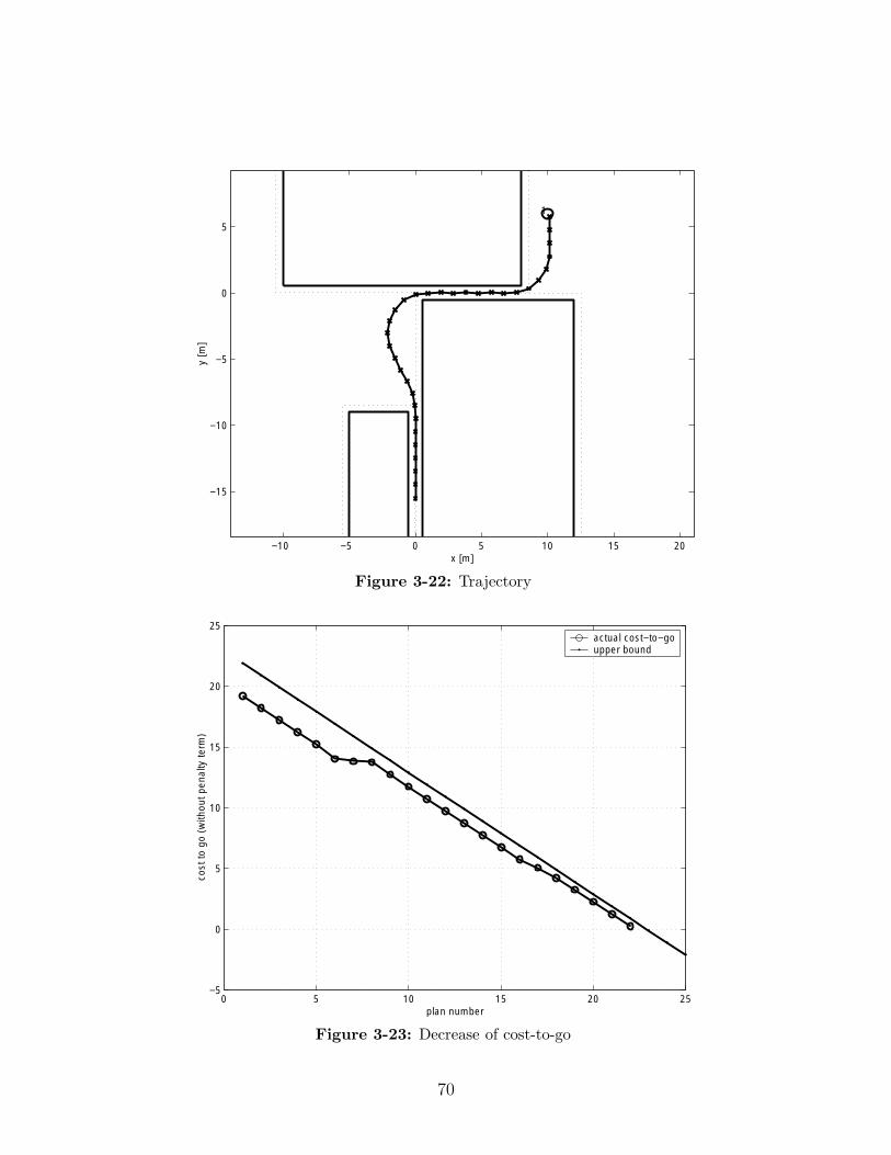
−10 −5 0 5 10 15 20

−15

−10

−5

0

5

x [m]

y [m

]1

Figure 3-22: Trajectory

0 5 10 15 20 25−5

0

5

10

15

20

25

plan number

cost

to g

o (w

ithou

t pen

alty

term

)

actual cost−to−goupper bound

Figure 3-23: Decrease of cost-to-go

70

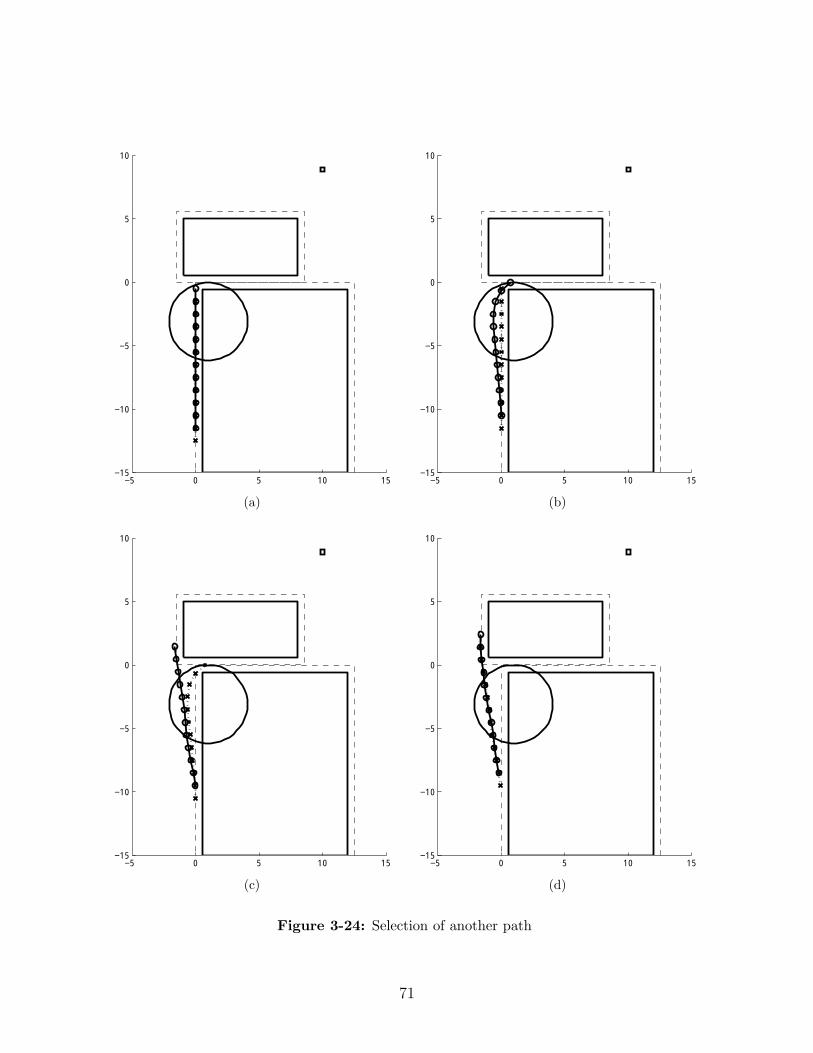
−5 0 5 10 15−15

−10

−5

0

5

10

(a)

−5 0 5 10 15−15

−10

−5

0

5

10

(b)

−5 0 5 10 15−15

−10

−5

0

5

10

(c)

−5 0 5 10 15−15

−10

−5

0

5

10

(d)

Figure 3-24: Selection of another path

71

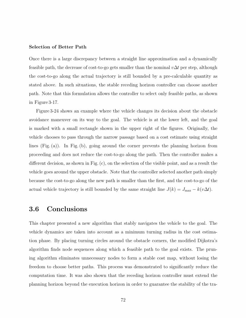
Selection of Better Path

Once there is a large discrepancy between a straight line approximation and a dynamically

feasible path, the decrease of cost-to-go gets smaller than the nominal v∆t per step, although

the cost-to-go along the actual trajectory is still bounded by a pre-calculable quantity as

stated above. In such situations, the stable receding horizon controller can choose another

path. Note that this formulation allows the controller to select only feasible paths, as shown

in Figure 3-17.

Figure 3-24 shows an example where the vehicle changes its decision about the obstacle

avoidance maneuver on its way to the goal. The vehicle is at the lower left, and the goal

is marked with a small rectangle shown in the upper right of the figures. Originally, the

vehicle chooses to pass through the narrow passage based on a cost estimate using straight

lines (Fig. (a)). In Fig. (b), going around the corner prevents the planning horizon from

proceeding and does not reduce the cost-to-go along the path. Then the controller makes a

different decision, as shown in Fig. (c), on the selection of the visible point, and as a result the

vehicle goes around the upper obstacle. Note that the controller selected another path simply

because the cost-to-go along the new path is smaller than the first, and the cost-to-go of the

actual vehicle trajectory is still bounded by the same straight line J(k) = Jmax − k(v∆t).

3.6 Conclusions

This chapter presented a new algorithm that stably navigates the vehicle to the goal. The

vehicle dynamics are taken into account as a minimum turning radius in the cost estima-

tion phase. By placing turning circles around the obstacle corners, the modified Dijkstra’s

algorithm finds node sequences along which a feasible path to the goal exists. The prun-

ing algorithm eliminates unnecessary nodes to form a stable cost map, without losing the

freedom to choose better paths. This process was demonstrated to significantly reduce the

computation time. It was also shown that the receding horizon controller must extend the

planning horizon beyond the execution horizon in order to guarantee the stability of the tra-

72

jectory optimization. The lower bound of the margin required was analytically calculated.

Combined with the stable cost map, this formulation proved that: 1) the RHC always has a

feasible solution, and 2) the vehicle reaches the goal in finite time. The simulations verified

these results.

73

74

Chapter 4

Task allocation for Multiple UAVs

with Timing Constraints and

Loitering

This chapter describes methods for optimizing the task allocation problem for a fleet of

unmanned aerial vehicles (UAVs) with tightly coupled tasks and rigid relative timing con-

straints. The overall objective is to minimize the mission completion time for the fleet, and

the task assignment must account for differing UAV capabilities and obstacles (no-fly zones).

Loitering times are included as extra degrees of freedom in the problem to help meet the

timing constraints. The overall problem is formulated using mixed-integer linear program-

ming(MILP). Commercial software exists to obtain the globally optimal solution to these

problems. However, an approximate decomposition solution method is used to overcome

many computational issues for reasonable sized problems.

4.1 Problem Formulation

This section describes how the multiple vehicle routing problems with relative timing con-

straints and loitering can be written as a MILP. The algorithms assume that the team par-

75

titioning has already been performed, and that a set of tasks has been identified that must

be performed by the team. The next step is to assign specific tasks to the team members

and design a detailed trajectory for each member to achieve these tasks.

4.1.1 Problem Statement

Let there be a team of NV UAVs with known starting states and maximum velocities, NW

waypoints1, and NZ no-fly zone. The starting state of the ith UAV is given by the ith row

[ x0i y0i x0i y0i ] of the NV ×4 matrix S0, and the maximum velocity of UAV i is given by

vmax,i. The locations of the NW waypoints are assumed to be known, and the (x, y) position

of waypoint i is given by the ith row [ Wi1 Wi2 ] of the matrix W. The (x, y) location of

the lower-left corner of the jth obstacle is given by (Zj1, Zj2), and the upper-right corner by

(Zj3, Zj4). Together, these two pairs make up the jth row of the NZ × 4 matrix Z.

The UAV capabilities are represented by the NV × NW binary capability matrix K.

The entry Kij is 1 if UAV i is capable of performing the tasks associated with waypoint

j, and 0 if not. Finally, NC timing constraints are in matrix C and vector d, in which

each row represents a dependency between two waypoints. A row k in C with [ i j ] and

corresponding element dk implies a timing constraint that waypoint j must be visited at

least dk time units after waypoint i.

The algorithm produces a trajectory for each UAV, represented for the ith UAV by a

series of states sti = [ xti yti xti yti ], t ∈ [1, tFi], where tFi

is the time at which UAV i

reaches its final waypoint. The finishing times of all UAVs make up the vector tF.

4.1.2 Algorithm Overview

There are three main phases in our algorithm [3, 4]: (I) cost calculation, (II) planning and

pruning, and (III) task assignment.

1In this chapter, “waypoint” refers to target or site to be visited whereas in the other chapters it refersto trajectory points generated by RHC.

76

I-1. Find the visibility graph between the UAV starting positions, waypoints, and

obstacle vertices.

I-2. Using the Dijkstra’s algorithm, calculate the shortest length of the all feasible

paths between waypoints, and form the cost table. The straight line length

divided by maximum velocity is used as an approximate cost.

II-1. Obtain feasible combinations of waypoints, accounting for the capability matrix

K and the maximum number of waypoints per UAV.

II-2. Enumerate all feasible permutations from these combinations, subject to the

timing constraints.

II-3. Calculate cost for each permutation using the cost table obtained in phase I.

II-4. Select the np best permutations for each combination. Typically, setting np = 1

will yield the optimal solution to the assignment problem.

III-1. Solve the task allocation problem using an optimization solver.

III-2. Solve for the each UAV’s trajectory (e.g. using straight line segments).

At the end of the phase II, four matrices are produced whose jth columns, taken together,

fully describe one permutation of waypoints. These are the row vector u, whose uj entry

identifies which UAV is involved in the jth permutation; NW × NM matrix V, whose Vij

entry is 1 if waypoint i is visited by permutation j, and 0 if not; NW ×NM matrix T, whose

Tij entry is the time at which waypoint i is visited by permutation j assuming there is no

loitering, and 0 if waypoint i is not visited; and the row vector c, whose cj entry is the

completion time for the jth permutation, again, assuming there is no loitering. All of the

permutations produced by this algorithm are guaranteed to be feasible given the associated

UAV’s capabilities.

4.1.3 Decision Variables

The overall objective is to assign one set of ordered waypoints to each vehicle that is combined

into the mission plan, and adjust the loiter times for the team such that the cost of the mission

is minimized and the time of task execution at each waypoint satisfies the timing constraints.

77

Selection of the Permutations:

In order to assign one permutation to one vehicle, the NM × 1 binary decision vector x isintroduced whose xj equals one if permutation j is selected, and 0 otherwise. Each waypoint

must be visited once, and each vehicle must be assigned to one permutation, so

NM∑j=1

Vijxj = 1 , i = 1, . . . , NW (4.1)

Np+1−1∑j=Np

xj = 1 , p = 1, . . . , NV (4.2)

where the permutations of pth vehicle are numbered Np to Np+1 − 1, with N1 = 1 and

NNV +1 = NM + 1.

Loitering time:

We introduce the NW ×NV loitering matrix L, whose Lij element expresses the loiter time

at the ith waypoint when visited by UAV j, as a set of new decision variables. Lij = 0 if

waypoint i is not visited by UAV j. This loitering matrix ensures that it is always possible

to find a feasible solution as long as the timing constraints are consistent. In the MILP

formulation, the time of the task execution at waypoint i, TOE i, is written as

TOE i =NM∑j=1

Tij xj + LB i , i = 1, . . . , NW (4.3)

where the first term expresses the flight time from the start point to waypoint i at vmax, and

LB i is the sum of the loiter times before executing the task at waypoint i.

As shown in Fig. 4-1, the loiter time at waypoint i is defined as the time difference between

time of the task execution and the time of arrival at waypoint i. The UAVs are assumed to fly

at the maximum speed between waypoints, and loiter before executing the task. Note that

this formulation only allows loitering at waypoints, but it can also be regarded as flying at

a slower speed between the waypoints, or loitering at the previous waypoint, flying towards

78

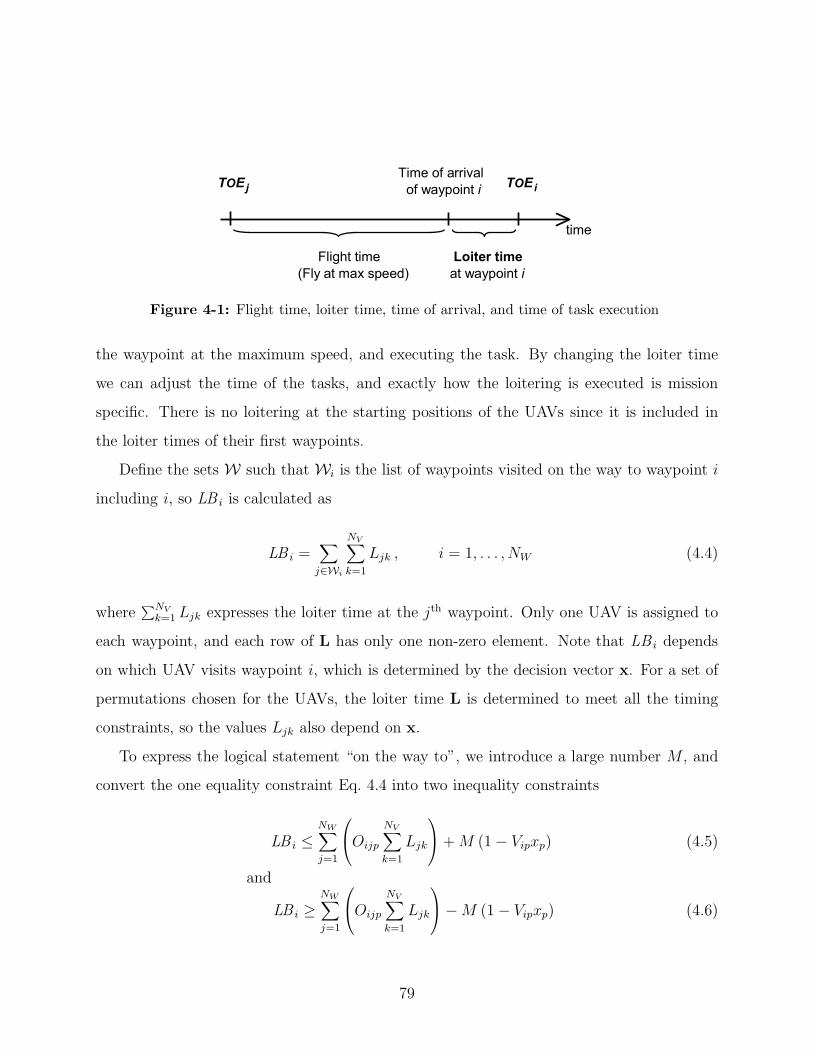
Time of arrival

Loiter time

(Fly at max speed)

TOEj of waypoint i

Flight time

TOEi

at waypoint i

time

Figure 4-1: Flight time, loiter time, time of arrival, and time of task execution

the waypoint at the maximum speed, and executing the task. By changing the loiter time

we can adjust the time of the tasks, and exactly how the loitering is executed is mission

specific. There is no loitering at the starting positions of the UAVs since it is included in

the loiter times of their first waypoints.

Define the sets W such that Wi is the list of waypoints visited on the way to waypoint i

including i, so LB i is calculated as

LB i =∑j∈Wi

NV∑k=1

Ljk , i = 1, . . . , NW (4.4)

where∑NV

k=1 Ljk expresses the loiter time at the jth waypoint. Only one UAV is assigned to

each waypoint, and each row of L has only one non-zero element. Note that LB i depends

on which UAV visits waypoint i, which is determined by the decision vector x. For a set of

permutations chosen for the UAVs, the loiter time L is determined to meet all the timing

constraints, so the values Ljk also depend on x.

To express the logical statement “on the way to”, we introduce a large number M , and

convert the one equality constraint Eq. 4.4 into two inequality constraints

LB i ≤NW∑j=1

Oijp

NV∑k=1

Ljk

+M (1− Vipxp) (4.5)

and

LB i ≥NW∑j=1

Oijp

NV∑k=1

Ljk

−M (1− Vipxp) (4.6)

79

where O is a three dimensional binary matrix that expresses waypoint orderings, and its Oijp

entry is 1 if waypoint j is visited before waypoint i (including i = j) by permutation p, and 0

if not. When waypoint i is visited by permutation p, the second term on the right-hand side

of the constraints in Eq. 4.5 and 4.6 disappear since∑NM

p=1 Vipxp = 1. In that case, Eq. 4.5

and 4.6 can be combined to form the equality constraint

LB i =NW∑j=1

Oijp

NV∑k=1

Ljk

(4.7)

which is the same as Eq. 4.4. Note that when waypoint i is not visited by permutation p,

Oijp = 0 for all j and Vip = 0, so that both of the inequality constraints are relaxed and LB i

is not constrained.

4.1.4 Timing Constraints

The timing constraints of interest in this application are relative, as opposed to the absolute

ones often considered [28, 29, 30, 31, 32]. The constraints can be written as

TOECk2≥ TOECk1

+ dk , k = 1, . . . , NC (4.8)

yielding a very general formulation. Recall matrixC contains indices of waypoints involved in

each timing constraint k. If the kth row of C is [ i j ], Eq. 4.8 becomes TOE j ≥ TOE i+dk.

Note that dk can also be negative. This formulation allows us to describe all kinds of

timing constraints. For example, although each waypoint i has only one time of execution

TOE i associated with it, this formulation can be used to describe several visits with timing

constraints by putting multiple waypoints at that location.

80

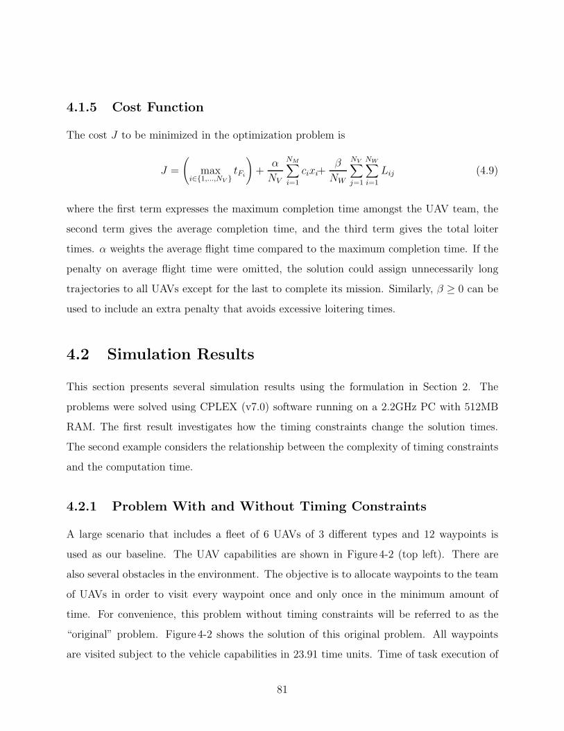
4.1.5 Cost Function

The cost J to be minimized in the optimization problem is

J =

(max

i∈{1,...,NV }tFi

)+α

NV

NM∑i=1

cixi+β

NW

NV∑j=1

NW∑i=1

Lij (4.9)

where the first term expresses the maximum completion time amongst the UAV team, the

second term gives the average completion time, and the third term gives the total loiter

times. α weights the average flight time compared to the maximum completion time. If the

penalty on average flight time were omitted, the solution could assign unnecessarily long

trajectories to all UAVs except for the last to complete its mission. Similarly, β ≥ 0 can be

used to include an extra penalty that avoids excessive loitering times.

4.2 Simulation Results

This section presents several simulation results using the formulation in Section 2. The

problems were solved using CPLEX (v7.0) software running on a 2.2GHz PC with 512MB

RAM. The first result investigates how the timing constraints change the solution times.

The second example considers the relationship between the complexity of timing constraints

and the computation time.

4.2.1 Problem With and Without Timing Constraints

A large scenario that includes a fleet of 6 UAVs of 3 different types and 12 waypoints is

used as our baseline. The UAV capabilities are shown in Figure 4-2 (top left). There are

also several obstacles in the environment. The objective is to allocate waypoints to the team

of UAVs in order to visit every waypoint once and only once in the minimum amount of

time. For convenience, this problem without timing constraints will be referred to as the

“original” problem. Figure 4-2 shows the solution of this original problem. All waypoints

are visited subject to the vehicle capabilities in 23.91 time units. Time of task execution of

81

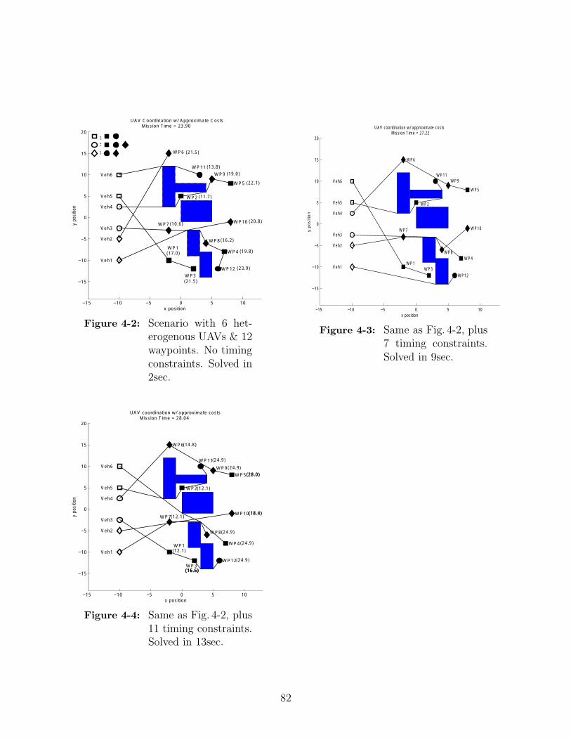
−15 −10 −5 0 5 10

−15

−10

−5

0

5

10

15

20

WP1

WP2

WP3

WP4

WP5

WP6

WP7

WP8

WP9

WP10

WP11

WP12

Veh1

Veh2

Veh3

Veh4

Veh5

Veh6

x position

y po

sitio

n

UAV Coordination w/ Approximate Costs Mission Time = 23.90

: : :

(17.0)

(11.7)

(21.5)

(19.8)

(22.1)

(21.5)

(10.6)

(16.2)

(19.0)

(20.8)

(13.8)

(23.9)

Figure 4-2: Scenario with 6 het-erogenous UAVs & 12waypoints. No timingconstraints. Solved in2sec.

−15 −10 −5 0 5 10

−15

−10

−5

0

5

10

15

20

WP1

WP2

WP3

WP4

WP5

WP6

WP7

WP8

WP9

WP10

WP11

WP12

Veh1

Veh2

Veh3

Veh4

Veh5

Veh6

x positiony p

ositio

n

UAV coordination w/ approximate costs Mission Time = 27.22

Figure 4-3: Same as Fig. 4-2, plus7 timing constraints.Solved in 9sec.

−15 −10 −5 0 5 10

−15

−10

−5

0

5

10

15

20

WP1

WP2

WP3

WP4

WP5

WP6

WP7

WP8

WP9

WP10

WP11

WP12

Veh1

Veh2

Veh3

Veh4

Veh5

Veh6

x position

y po

sitio

n

UAV coordination w/ approximate costs Mission Time = 28.04

(12.1)

(24.9)

(12.1)

(12.1)

(24.9)

(24.9)

(24.9)

(24.9)

(28.0) (28.0)

(18.4) (18.4)

(16.6) (16.6) (16.6)

(14.8)

Figure 4-4: Same as Fig. 4-2, plus11 timing constraints.Solved in 13sec.

82

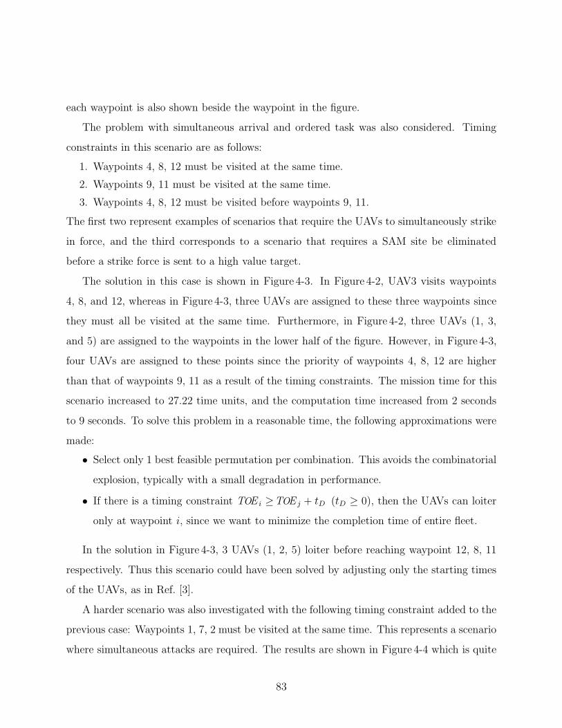
each waypoint is also shown beside the waypoint in the figure.

The problem with simultaneous arrival and ordered task was also considered. Timing

constraints in this scenario are as follows:

1. Waypoints 4, 8, 12 must be visited at the same time.

2. Waypoints 9, 11 must be visited at the same time.

3. Waypoints 4, 8, 12 must be visited before waypoints 9, 11.

The first two represent examples of scenarios that require the UAVs to simultaneously strike

in force, and the third corresponds to a scenario that requires a SAM site be eliminated

before a strike force is sent to a high value target.

The solution in this case is shown in Figure 4-3. In Figure 4-2, UAV3 visits waypoints

4, 8, and 12, whereas in Figure 4-3, three UAVs are assigned to these three waypoints since

they must all be visited at the same time. Furthermore, in Figure 4-2, three UAVs (1, 3,

and 5) are assigned to the waypoints in the lower half of the figure. However, in Figure 4-3,

four UAVs are assigned to these points since the priority of waypoints 4, 8, 12 are higher

than that of waypoints 9, 11 as a result of the timing constraints. The mission time for this

scenario increased to 27.22 time units, and the computation time increased from 2 seconds

to 9 seconds. To solve this problem in a reasonable time, the following approximations were

made:

• Select only 1 best feasible permutation per combination. This avoids the combinatorialexplosion, typically with a small degradation in performance.

• If there is a timing constraint TOE i ≥TOE j + tD (tD ≥ 0), then the UAVs can loiter

only at waypoint i, since we want to minimize the completion time of entire fleet.

In the solution in Figure 4-3, 3 UAVs (1, 2, 5) loiter before reaching waypoint 12, 8, 11

respectively. Thus this scenario could have been solved by adjusting only the starting times

of the UAVs, as in Ref. [3].

A harder scenario was also investigated with the following timing constraint added to the

previous case: Waypoints 1, 7, 2 must be visited at the same time. This represents a scenario

where simultaneous attacks are required. The results are shown in Figure 4-4 which is quite

83

Table 4.1: Results with no constraints on loitering time.

Case 1 2 3 4Avg. computation time (s) 3.3 20.6 4.6 23.9% of prob. solved in 5 sec 97.0 27.3 80.0 13.9

Table 4.2: Result with constrained loitering times.

Case 1 2 3 4Avg. computation time (s) 2.2 8.5 3.0 11.6% of prob. solved in 5 sec 100.0 48.4 93.0 30.3

different from Figure 4-3 (e.g. Waypoint 4 is visited by UAV6, which is the farthest from it).

In order to satisfy the many timing constraints, 4 UAVs loiter at 6 waypoints. UAV1 loiters

on its way to waypoint 7 and 8, and UAV3 loiters on its way to waypoints 1 and 12. If time

adjustment is allowed only on the initial position, a feasible solution cannot be found in this

scenario. Since the loiter matrix L allows UAVs to loiter at any of the waypoints with timing

constraints, problems with strongly coupled timing constraints are always solvable.

4.2.2 Complexity of Adding Timing Constraints

To investigate the impact of the timing constraints on the performance and computation

time, we measured the computation time for the same problem in Section 4.2.1, with the

following 4 different cases of timing constraints:

Case – 1: TOE i ≥ TOE j

Case – 2: TOE i ≥ TOE j + 10

Case – 3: TOE i ≥ TOE j ≥ TOE k

Case – 4: TOE i ≥ TOE j + 5 ≥ TOE k + 10

In each case, all feasible combinations of waypoints (i, j) or (i, j, k) were tested as the

points associated with the timing constraints. The results are summarized in the histograms

of Figures 4-5–4-8 and Tables 4.1 and 4.2.

Figures 4-5(a), 4-6(a), 4-7(a), and 4-8(a) show the results when all loitering times are

included in the problem. Since there are 12 waypoints and 6 UAVs with different capabiilties,

84

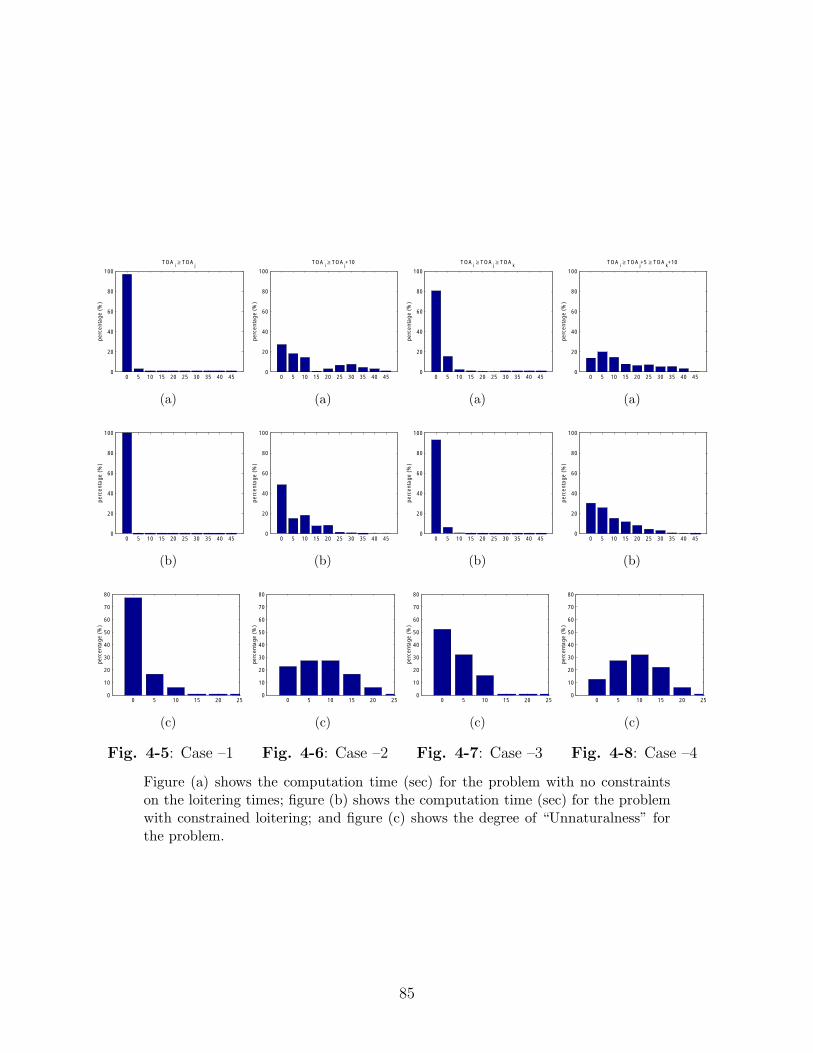
0 5 10 15 20 25 30 35 40 450

20

40

60

80

100

TOA i ≥ TOA

j

perc

enta

ge (

%)

(a)

0 5 10 15 20 25 30 35 40 450

20

40

60

80

100

perc

enta

ge (

%)

(b)

0 5 10 15 20 250

10

20

30

40

50

60

70

80

perc

enta

ge (

%)

(c)

Fig. 4-5: Case –1

0 5 10 15 20 25 30 35 40 450

20

40

60

80

100

TOA i ≥ TOA

j+10

perc

enta

ge (

%)

(a)

0 5 10 15 20 25 30 35 40 450

20

40

60

80

100

perc

enta

ge (

%)

(b)

0 5 10 15 20 250

10

20

30

40

50

60

70

80

perc

enta

ge (

%)

(c)

Fig. 4-6: Case –2

0 5 10 15 20 25 30 35 40 450

20

40

60

80

100

TOA i ≥ TOA

j ≥ TOA

k

perc

enta

ge (

%)

(a)

0 5 10 15 20 25 30 35 40 450

20

40

60

80

100

perc

enta

ge (

%)

(b)

0 5 10 15 20 250

10

20

30

40

50

60

70

80

perc

enta

ge (

%)

(c)

Fig. 4-7: Case –3

0 5 10 15 20 25 30 35 40 450

20

40

60

80

100

TOA i ≥ TOA

j+5 ≥ TOA

k+10

perc

enta

ge (

%)

(a)

0 5 10 15 20 25 30 35 40 450

20

40

60

80

100

perc

enta

ge (

%)

(b)

0 5 10 15 20 250

10

20

30

40

50

60

70

80

perc

enta

ge (

%)

(c)

Fig. 4-8: Case –4

Figure (a) shows the computation time (sec) for the problem with no constraintson the loitering times; figure (b) shows the computation time (sec) for the problemwith constrained loitering; and figure (c) shows the degree of “Unnaturalness” forthe problem.

85

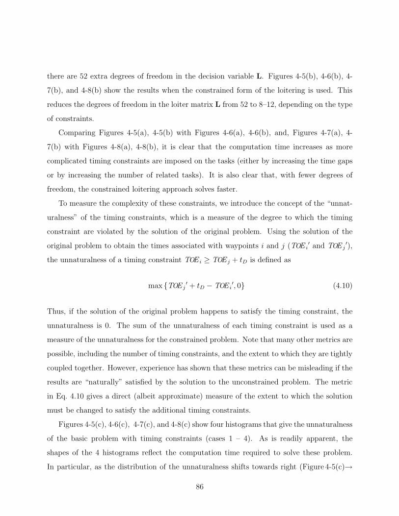
there are 52 extra degrees of freedom in the decision variable L. Figures 4-5(b), 4-6(b), 4-

7(b), and 4-8(b) show the results when the constrained form of the loitering is used. This

reduces the degrees of freedom in the loiter matrix L from 52 to 8–12, depending on the type

of constraints.

Comparing Figures 4-5(a), 4-5(b) with Figures 4-6(a), 4-6(b), and, Figures 4-7(a), 4-

7(b) with Figures 4-8(a), 4-8(b), it is clear that the computation time increases as more

complicated timing constraints are imposed on the tasks (either by increasing the time gaps

or by increasing the number of related tasks). It is also clear that, with fewer degrees of

freedom, the constrained loitering approach solves faster.

To measure the complexity of these constraints, we introduce the concept of the “unnat-

uralness” of the timing constraints, which is a measure of the degree to which the timing

constraint are violated by the solution of the original problem. Using the solution of the

original problem to obtain the times associated with waypoints i and j (TOE i′ and TOE j

′),

the unnaturalness of a timing constraint TOE i ≥ TOE j + tD is defined as

max {TOE j′ + tD − TOE i

′, 0} (4.10)

Thus, if the solution of the original problem happens to satisfy the timing constraint, the

unnaturalness is 0. The sum of the unnaturalness of each timing constraint is used as a

measure of the unnaturalness for the constrained problem. Note that many other metrics are

possible, including the number of timing constraints, and the extent to which they are tightly

coupled together. However, experience has shown that these metrics can be misleading if the

results are “naturally” satisfied by the solution to the unconstrained problem. The metric

in Eq. 4.10 gives a direct (albeit approximate) measure of the extent to which the solution

must be changed to satisfy the additional timing constraints.

Figures 4-5(c), 4-6(c), 4-7(c), and 4-8(c) show four histograms that give the unnaturalness

of the basic problem with timing constraints (cases 1 – 4). As is readily apparent, the

shapes of the 4 histograms reflect the computation time required to solve these problem.

In particular, as the distribution of the unnaturalness shifts towards right (Figure 4-5(c)→

86

4-6(c) and 4-7(c)→ 4-8(c)), the distribution of the computation time also shifts to the right

(Figure 4-5(b)→ 4-6(b) and 4-7(b)→ 4-8(b)). Further observations include:

• If all of the timing constraints are natural, then the computation time does not increasesignificantly, even if there are many timing constraints.

• Infeasible permutations must be pruned before the cost calculation of each permutation,so that the best permutation for each combination is always feasible. If all the timing

constraints are natural, the best permutation is always feasible without pruning by

timing constraints, but that is not the case if there are unnatural timing constraints.

• Additional permutations can be kept to account for unnatural timing constraints, butsimulation results have shown that this can rapidly increase the computational time

with a marginal improvement in performance.

4.3 Conclusions

This chapter presented an extension of the multiple UAV task allocation problem that ex-

plicitly includes the relative timing constraints found in many mission scenarios. This not

only allows us to determine which vehicle should go to each waypoint, but it also allows

us to account for the required ordering and relative timing in the task assignment. The

allocation problem was also extended to include loiter times as extra (continuous) degrees of

freedom to ensure that, even with very complicated timing constraints, feasible solutions still

exist. Simulation results clearly showed that adding these timing constraints to the problem

increases the computational time when the constraints are active (i.e., “unnatural”).

This formulation becomes computationally intractable for reasonable sized problems.

However, it is shown that an approximate decomposition solution method can be used to

overcome many of these computational issues and solve problems with highly coupled tasks

and timing constraints.

87

88

Chapter 5

Hardware Experiments

This chapter presents several results of hardware experiments with the receding horizon con-

troller (RHC) discussed in the previous chapters. Section 5.1 describes the assumptions on

which the experiments are based, and clarifies the difference between MATLAB simulations

and the real world experiments. Section 5.2 shows the testbed setup and how the RHC

interacts with the real world through the hardware. Two key features of RHC are demon-

strated in Sections 5.3 to 5.5: replanning to account for uncertainty in the environment and

real-time trajectory generation. In particular, Section 5.3 integrates the on-board low-level

feedback controller and the RHC. Section 5.4 examines the replanning capability of the re-

ceding horizon trajectory generation. Section 5.5 considers a scenario with a large change in

the situational awareness that requires on-line reassignment of tasks among the vehicles.

5.1 Experiments Overview

This section gives an overview of the experiments presented in this chapter. Figure 5-1 shows

a hierarchical approach to the control and coordination of multiple vehicles. In the following

experiments, the planner, which is shown as a box with dashed lines in the figure, interacts

with the real environment. Four different levels of control loops are closed, one at a time, in

Section 5.2 to Section 5.5, which are shown as grey boxes in the figure.

89

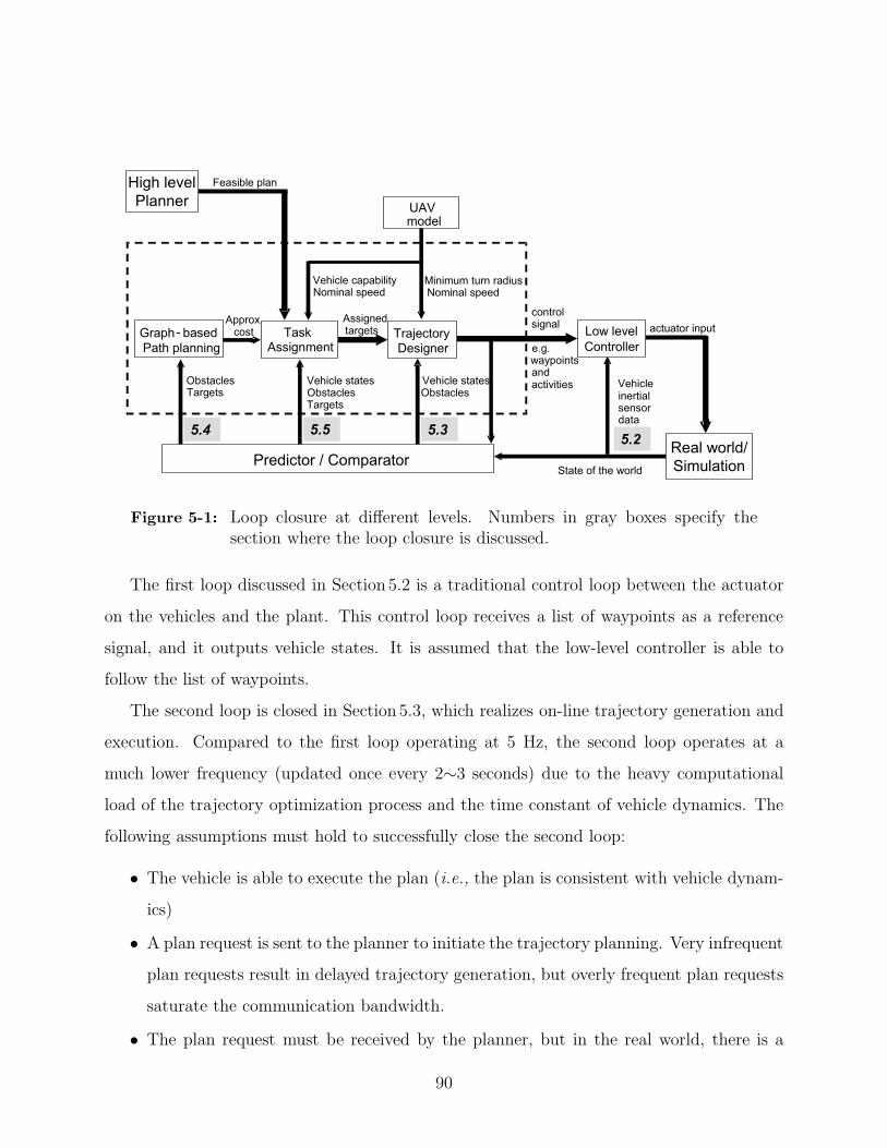
actuator inputAssignedtargets

Minimum turn radiusNominal speed

UAVmodel

Vehicle statesObstaclesTargets

Vehicle statesObstacles

controlsignal

e.g.waypoints and activities

Vehicle capabilityNominal speed

Vehicleinertialsensordata

State of the worldPredictor / Comparator

Real world/

Simulation

ObstaclesTargets

Approx. cost

High level

Planner

Feasible plan

Low level

ControllerTrajectoryDesigner

Graph- based

Path planning

Task Assignment

5.35.35.55.55.45.45.25.2

Figure 5-1: Loop closure at different levels. Numbers in gray boxes specify thesection where the loop closure is discussed.

The first loop discussed in Section 5.2 is a traditional control loop between the actuator

on the vehicles and the plant. This control loop receives a list of waypoints as a reference

signal, and it outputs vehicle states. It is assumed that the low-level controller is able to

follow the list of waypoints.

The second loop is closed in Section 5.3, which realizes on-line trajectory generation and

execution. Compared to the first loop operating at 5 Hz, the second loop operates at a

much lower frequency (updated once every 2∼3 seconds) due to the heavy computationalload of the trajectory optimization process and the time constant of vehicle dynamics. The

following assumptions must hold to successfully close the second loop:

• The vehicle is able to execute the plan (i.e., the plan is consistent with vehicle dynam-ics)

• A plan request is sent to the planner to initiate the trajectory planning. Very infrequentplan requests result in delayed trajectory generation, but overly frequent plan requests

saturate the communication bandwidth.

• The plan request must be received by the planner, but in the real world, there is a

90

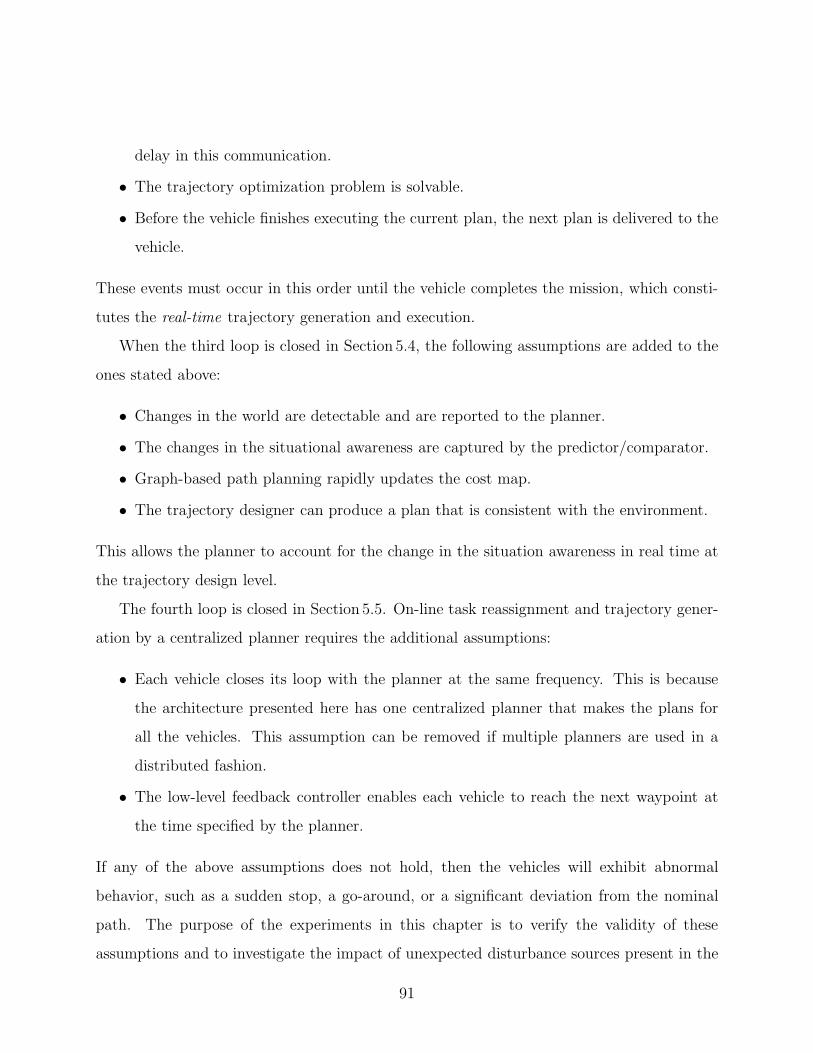
delay in this communication.

• The trajectory optimization problem is solvable.

• Before the vehicle finishes executing the current plan, the next plan is delivered to thevehicle.

These events must occur in this order until the vehicle completes the mission, which consti-

tutes the real-time trajectory generation and execution.

When the third loop is closed in Section 5.4, the following assumptions are added to the

ones stated above:

• Changes in the world are detectable and are reported to the planner.• The changes in the situational awareness are captured by the predictor/comparator.• Graph-based path planning rapidly updates the cost map.• The trajectory designer can produce a plan that is consistent with the environment.

This allows the planner to account for the change in the situation awareness in real time at

the trajectory design level.

The fourth loop is closed in Section 5.5. On-line task reassignment and trajectory gener-

ation by a centralized planner requires the additional assumptions:

• Each vehicle closes its loop with the planner at the same frequency. This is becausethe architecture presented here has one centralized planner that makes the plans for

all the vehicles. This assumption can be removed if multiple planners are used in a

distributed fashion.

• The low-level feedback controller enables each vehicle to reach the next waypoint atthe time specified by the planner.

If any of the above assumptions does not hold, then the vehicles will exhibit abnormal

behavior, such as a sudden stop, a go-around, or a significant deviation from the nominal

path. The purpose of the experiments in this chapter is to verify the validity of these

assumptions and to investigate the impact of unexpected disturbance sources present in the

91

Vehicle

Controller

Plan (waypoints)

Vehicle

Controller

Vehicle

Controller

Vehicle statesBrain

Plan (waypoints)

Targets,

Vehicle states,

Obstacles

<Wireless LAN><Wireless LAN><LAN (TCP/IP)><LAN (TCP/IP)>

Planner

RHC

Task

Assignment

Graph

Search

Figure 5-2: Planner and hardware integration

real world that the simulation fails to capture. This is accomplished by showing the testbeds

controlled by the planning algorithm in real time with all loops closed.

5.2 Hardware Setup

This section describes two testbeds that were built to test the planning algorithms dis-

cussed in the previous chapters. First of all, Section 5.2.1 discusses the waypoint follower

interface set up between the receding horizon trajectory designer and the two testbeds. In

Section 5.2.2, the truck system is discussed as a ground-based testbed [33]. Section 5.2.3

describes the UAV testbed, which uses autopilots in a hardware-in-the-loop simulation.

5.2.1 Interface Setup

In the experimental demonstration, the RHC is used as a “high-level” controller to compen-

sate for uncertainty in the environment. It designs a series of waypoints for each vehicle

to follow. A “low-level” vehicle controller then steers the vehicle to move along this path.

Figure 5-2 shows an interface set up between the planner and the testbed.

There is a central data manager labelled “Brain” that monitors the vehicle positions

and sends plan requests to the planner, receives planned waypoints and sends them to each

truck, and simulates changes in situation awareness such as obstacle detection and discovery

92

of new targets. Currently sensors are not implemented on the testbeds, thus the brain creates

simulated sensor data based on the actual vehicle location. This allows us to evaluate how

the different types of sensors impact the planning algorithm without actually implementing

the hardware. This brain function fits in Figure 5-1 as a “Predictor/Comparator” block.

Both the ground-based truck and autopilot testbeds have the same interface to the plan-

ner, and the planning algorithm will be demonstrated on both. All of the data is exchanged

between the planner, brain, and testbed vehicles via TCP/IP local area network connections,

which can flexibly accommodate additional vehicles or another module such as a mission

level planner and GUI for a human operator. This LAN communication has a bandwidth of

10Mbps, which is high enough to send vehicle states and planned waypoints. The CPU of

the planner laptop is a Pentium IV 2.0GHz with 1 GB RAM, the fastest laptop available in

2002.

5.2.2 Truck Testbed

The truck testbed has been built with a view for future UAV control use. It represents

models of UAVs, which would typically operate at a constant, nominal speed, flying at a

fixed altitude, and with the turning rate limited by the achievable bank angle. The testbed

described here consists of three remote-controlled, wheel-steered miniature trucks, as shown

in Figure 5-3. In order to capture the characteristics of UAVs, they are operated at constant

speed. Due to the limited steering angles, the turn rate of the trucks is also restricted.

Figure 5-4 is a block diagram of the truck testbed. The central base station has a fixed

GPS antenna to enable differential GPS. Each truck has a Pentium III 850MHz laptop, a GPS

antenna, a GPS receiver, and a PWM board that converts commands from the laptop into

PWM commands for the steering and drive motors. Doppler velocity measurement provided

by the GPS NAVSTAR constellation has high accuracy (standard deviation of 1-2 mm/sec)

and is integrated to produce position measurement data [33, 34]. Each truck and base station

runs the same GPS estimation program and they communicate via a built-in wireless LAN.

This produces position estimates accurate to about 10 cm for the length of the experiments

93

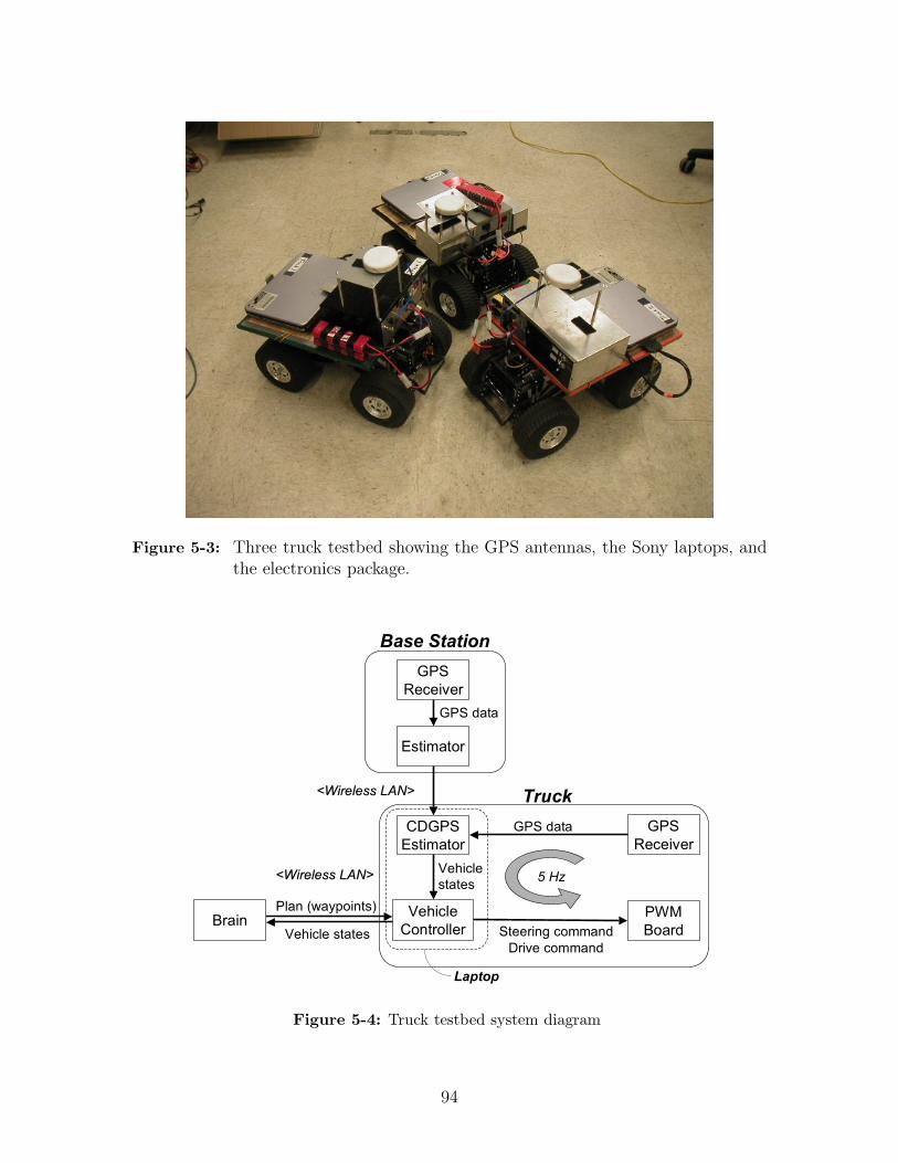
Figure 5-3: Three truck testbed showing the GPS antennas, the Sony laptops, andthe electronics package.

Vehicle

Controller

PWM

Board

GPS data GPS

Receiver

Steering command

Drive command

Plan (waypoints)

Vehicle states

Estimator

GPS

Receiver

GPS data

Base Station

Truck

CDGPS

Estimator

Vehicle

states5 Hz

Brain

<Wireless LAN><Wireless LAN>

<Wireless LAN><Wireless LAN>

Laptop

Figure 5-4: Truck testbed system diagram

94

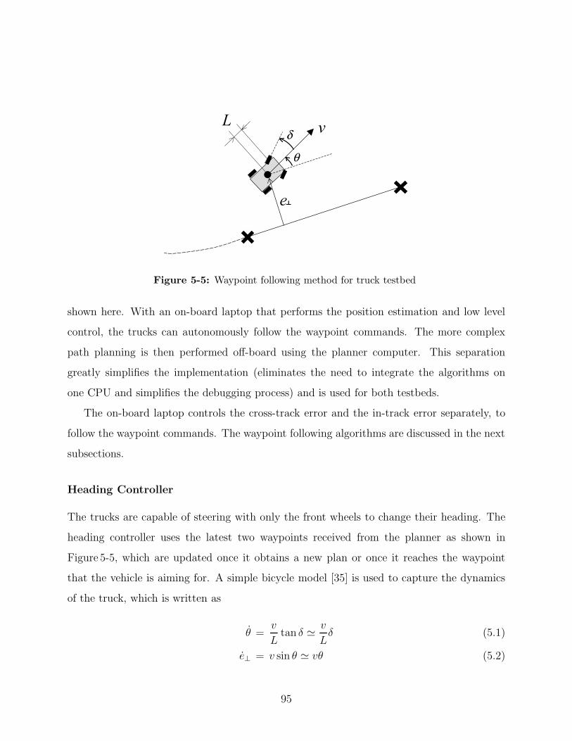
v

θ

e T

δL

Figure 5-5: Waypoint following method for truck testbed

shown here. With an on-board laptop that performs the position estimation and low level

control, the trucks can autonomously follow the waypoint commands. The more complex

path planning is then performed off-board using the planner computer. This separation

greatly simplifies the implementation (eliminates the need to integrate the algorithms on

one CPU and simplifies the debugging process) and is used for both testbeds.

The on-board laptop controls the cross-track error and the in-track error separately, to

follow the waypoint commands. The waypoint following algorithms are discussed in the next

subsections.

Heading Controller

The trucks are capable of steering with only the front wheels to change their heading. The

heading controller uses the latest two waypoints received from the planner as shown in

Figure 5-5, which are updated once it obtains a new plan or once it reaches the waypoint

that the vehicle is aiming for. A simple bicycle model [35] is used to capture the dynamics

of the truck, which is written as

θ =v

Ltan δ � v

Lδ (5.1)

e⊥ = v sin θ � vθ (5.2)

95

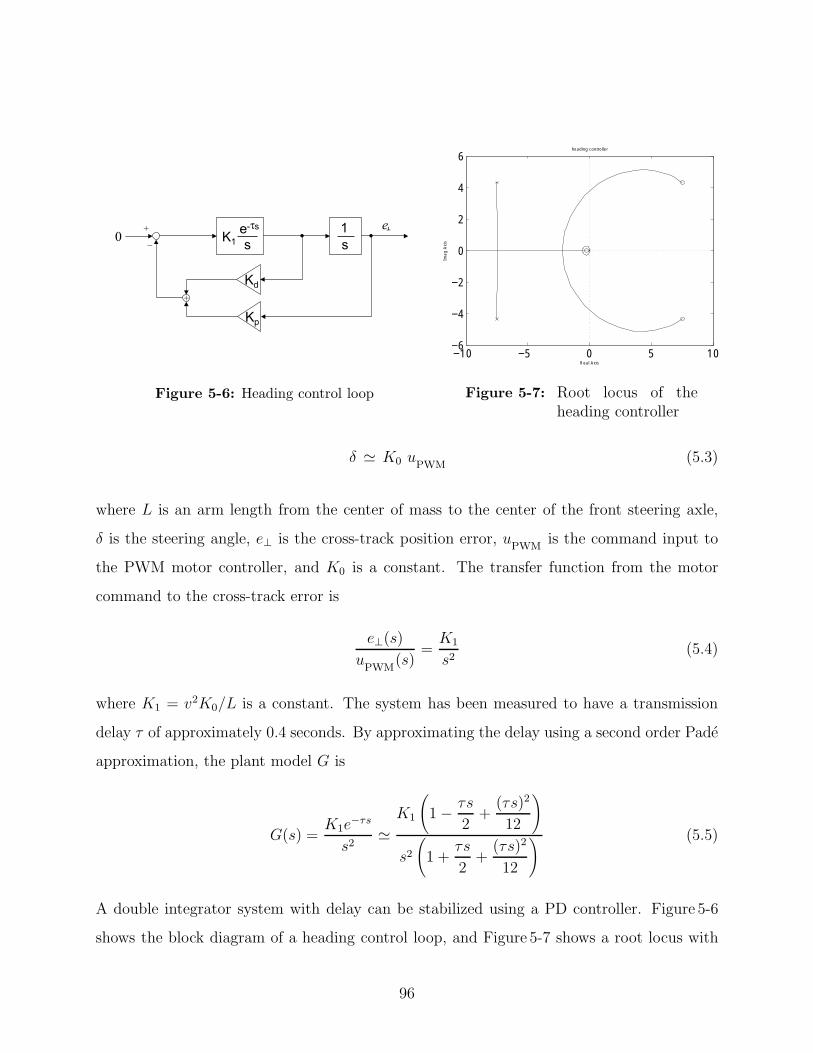
1

s

e-τs

s

Kd

Kp

+

–

+0

e T

K1

Figure 5-6: Heading control loop

heading controller

Real Axis

Imag

Axi

s

−10 −5 0 5 10−6

−4

−2

0

2

4

6

Figure 5-7: Root locus of theheading controller

δ � K0 uPWM(5.3)

where L is an arm length from the center of mass to the center of the front steering axle,

δ is the steering angle, e⊥ is the cross-track position error, uPWMis the command input to

the PWM motor controller, and K0 is a constant. The transfer function from the motor

command to the cross-track error is

e⊥(s)u

PWM(s)

=K1

s2(5.4)

where K1 = v2K0/L is a constant. The system has been measured to have a transmission

delay τ of approximately 0.4 seconds. By approximating the delay using a second order Pade

approximation, the plant model G is

G(s) =K1e

−τs

s2�K1

(1− τs

2+(τs)2

12

)

s2(1 +

τs

2+(τs)2

12

) (5.5)

A double integrator system with delay can be stabilized using a PD controller. Figure 5-6

shows the block diagram of a heading control loop, and Figure 5-7 shows a root locus with

96

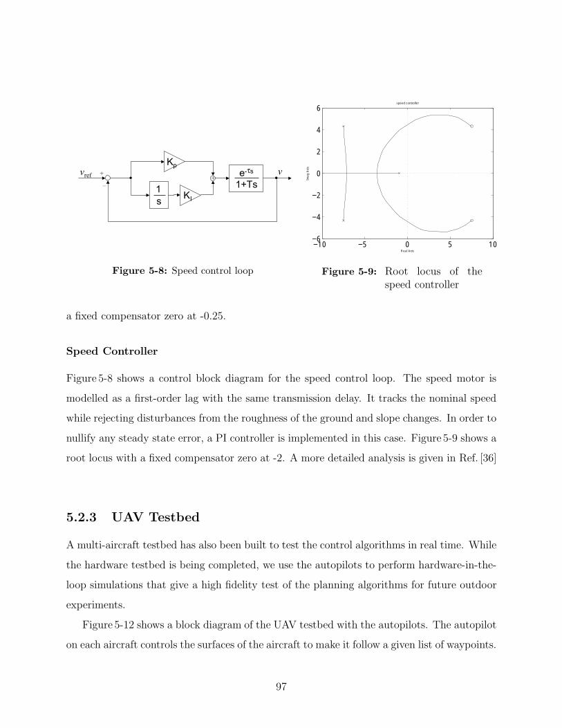
1

s

e-τs

1+TsKI

Kp

+–

+ vvref

Figure 5-8: Speed control loop

speed controller

Real Axis

Imag

Axi

s

−10 −5 0 5 10−6

−4

−2

0

2

4

6

Figure 5-9: Root locus of thespeed controller

a fixed compensator zero at -0.25.

Speed Controller

Figure 5-8 shows a control block diagram for the speed control loop. The speed motor is

modelled as a first-order lag with the same transmission delay. It tracks the nominal speed

while rejecting disturbances from the roughness of the ground and slope changes. In order to

nullify any steady state error, a PI controller is implemented in this case. Figure 5-9 shows a

root locus with a fixed compensator zero at -2. A more detailed analysis is given in Ref. [36]

5.2.3 UAV Testbed

A multi-aircraft testbed has also been built to test the control algorithms in real time. While

the hardware testbed is being completed, we use the autopilots to perform hardware-in-the-

loop simulations that give a high fidelity test of the planning algorithms for future outdoor

experiments.

Figure 5-12 shows a block diagram of the UAV testbed with the autopilots. The autopilot

on each aircraft controls the surfaces of the aircraft to make it follow a given list of waypoints.

97

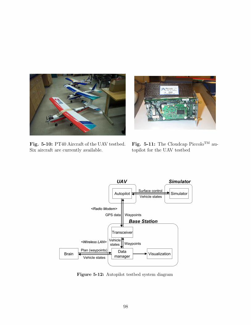
Fig. 5-10: PT40 Aircraft of the UAV testbed.Six aircraft are currently available.

Fig. 5-11: The Cloudcap PiccoloTM au-topilot for the UAV testbed

Transceiver

Autopilot

Data

managerVisualizationBrain

Plan (waypoints)

Vehicle states

GPS data

Base Station

UAV

Vehicle

states<Wireless LAN><Wireless LAN>

<Radio Modem><Radio Modem>

Simulator

SimulatorSurface control

Vehicle states

Waypoints

Waypoints

Figure 5-12: Autopilot testbed system diagram

98

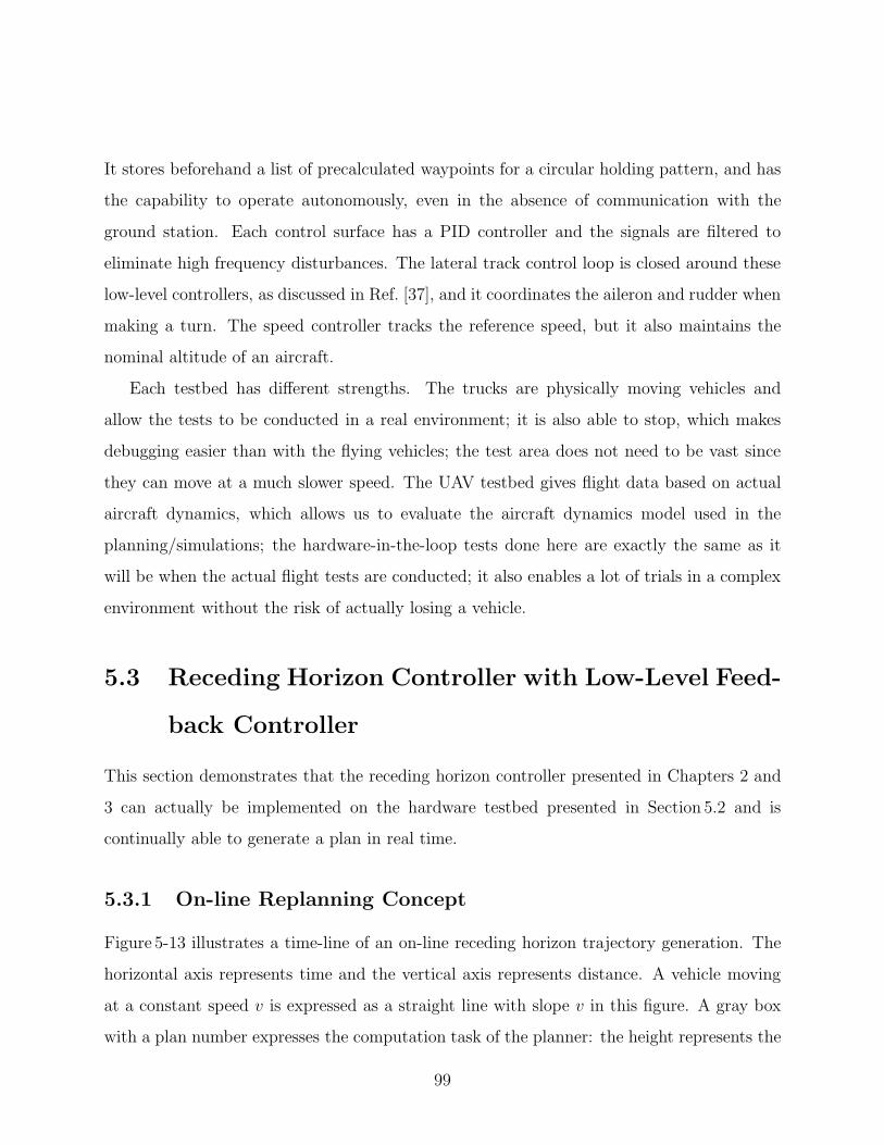
It stores beforehand a list of precalculated waypoints for a circular holding pattern, and has

the capability to operate autonomously, even in the absence of communication with the

ground station. Each control surface has a PID controller and the signals are filtered to

eliminate high frequency disturbances. The lateral track control loop is closed around these

low-level controllers, as discussed in Ref. [37], and it coordinates the aileron and rudder when

making a turn. The speed controller tracks the reference speed, but it also maintains the

nominal altitude of an aircraft.

Each testbed has different strengths. The trucks are physically moving vehicles and

allow the tests to be conducted in a real environment; it is also able to stop, which makes

debugging easier than with the flying vehicles; the test area does not need to be vast since

they can move at a much slower speed. The UAV testbed gives flight data based on actual

aircraft dynamics, which allows us to evaluate the aircraft dynamics model used in the

planning/simulations; the hardware-in-the-loop tests done here are exactly the same as it

will be when the actual flight tests are conducted; it also enables a lot of trials in a complex

environment without the risk of actually losing a vehicle.

5.3 Receding Horizon Controller with Low-Level Feed-

back Controller

This section demonstrates that the receding horizon controller presented in Chapters 2 and

3 can actually be implemented on the hardware testbed presented in Section 5.2 and is

continually able to generate a plan in real time.

5.3.1 On-line Replanning Concept

Figure 5-13 illustrates a time-line of an on-line receding horizon trajectory generation. The

horizontal axis represents time and the vertical axis represents distance. A vehicle moving

at a constant speed v is expressed as a straight line with slope v in this figure. A gray box

with a plan number expresses the computation task of the planner: the height represents the

99

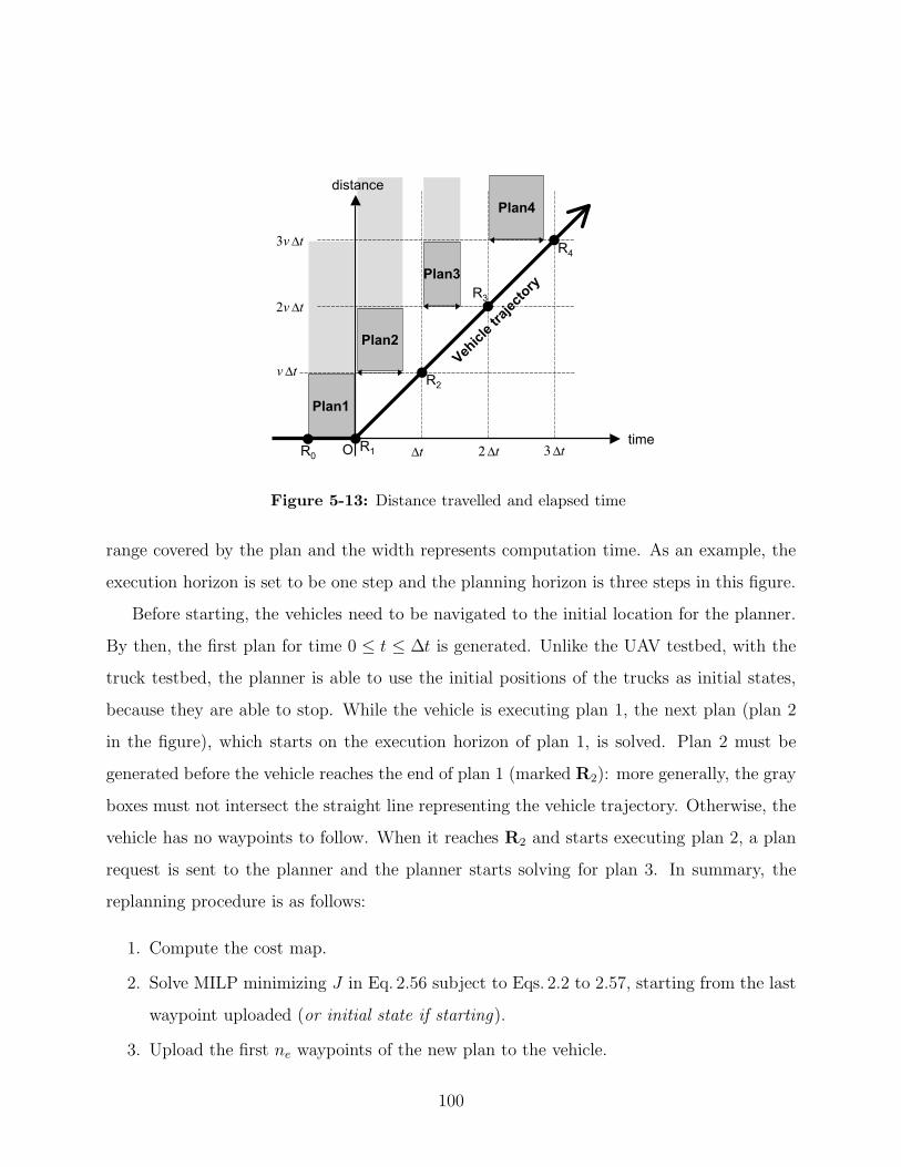
∆t 2 ∆t 3 ∆ttime

distance

Plan1

Plan2

Plan3

O

v∆t

2v∆t

3v∆t

Plan4

Veh

icle

traj

ecto

ry

R0R1

R2

R3

R4

Figure 5-13: Distance travelled and elapsed time

range covered by the plan and the width represents computation time. As an example, the

execution horizon is set to be one step and the planning horizon is three steps in this figure.

Before starting, the vehicles need to be navigated to the initial location for the planner.

By then, the first plan for time 0 ≤ t ≤ ∆t is generated. Unlike the UAV testbed, with the

truck testbed, the planner is able to use the initial positions of the trucks as initial states,

because they are able to stop. While the vehicle is executing plan 1, the next plan (plan 2

in the figure), which starts on the execution horizon of plan 1, is solved. Plan 2 must be

generated before the vehicle reaches the end of plan 1 (marked R2): more generally, the gray

boxes must not intersect the straight line representing the vehicle trajectory. Otherwise, the

vehicle has no waypoints to follow. When it reaches R2 and starts executing plan 2, a plan

request is sent to the planner and the planner starts solving for plan 3. In summary, the

replanning procedure is as follows:

1. Compute the cost map.

2. Solve MILP minimizing J in Eq. 2.56 subject to Eqs. 2.2 to 2.57, starting from the last

waypoint uploaded (or initial state if starting).

3. Upload the first ne waypoints of the new plan to the vehicle.

100

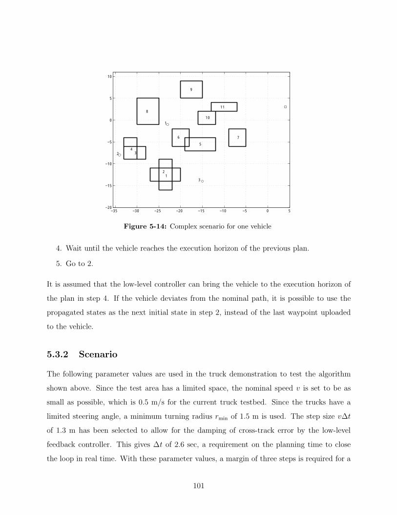
−35 −30 −25 −20 −15 −10 −5 0 5−20

−15

−10

−5

0

5

10

1

2

31

2

34

5

6 7

8

9

10

11

Figure 5-14: Complex scenario for one vehicle

4. Wait until the vehicle reaches the execution horizon of the previous plan.

5. Go to 2.

It is assumed that the low-level controller can bring the vehicle to the execution horizon of

the plan in step 4. If the vehicle deviates from the nominal path, it is possible to use the

propagated states as the next initial state in step 2, instead of the last waypoint uploaded

to the vehicle.

5.3.2 Scenario

The following parameter values are used in the truck demonstration to test the algorithm

shown above. Since the test area has a limited space, the nominal speed v is set to be as

small as possible, which is 0.5 m/s for the current truck testbed. Since the trucks have a

limited steering angle, a minimum turning radius rmin of 1.5 m is used. The step size v∆t

of 1.3 m has been selected to allow for the damping of cross-track error by the low-level

feedback controller. This gives ∆t of 2.6 sec, a requirement on the planning time to close

the loop in real time. With these parameter values, a margin of three steps is required for a

101

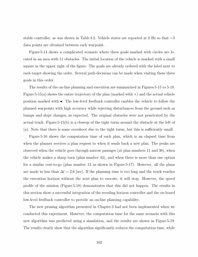
stable controller, as was shown in Table 3.2. Vehicle states are reported at 2 Hz so that ∼5data points are obtained between each waypoint.

Figure 5-14 shows a complicated scenario where three goals marked with circles are lo-

cated in an area with 11 obstacles. The initial location of the vehicle is marked with a small

square in the upper right of the figure. The goals are already ordered with the label next to

each target showing the order. Several path decisions can be made when visiting these three

goals in this order.

The results of the on-line planning and execution are summarized in Figures 5-15 to 5-18.

Figure 5-15(a) shows the entire trajectory of the plan (marked with ×) and the actual vehicleposition marked with •. The low-level feedback controller enables the vehicle to follow theplanned waypoints with high accuracy while rejecting disturbances from the ground such as

bumps and slope changes, as expected. The original obstacles were not penetrated by the

actual truck. Figure 5-15(b) is a closeup of the tight turns around the obstacle at the left of

(a). Note that there is some overshoot due to the tight turns, but this is sufficiently small.

Figure 5-16 shows the computation time of each plan, which is an elapsed time from

when the planner receives a plan request to when it sends back a new plan. The peaks are

observed when the vehicle goes through narrow passages (at plan numbers 11 and 38), when

the vehicle makes a sharp turn (plan number 34), and when there is more than one option

for a similar cost-to-go (plan number 13 as shown in Figure 5-17). However, all the plans

are made in less than ∆t = 2.6 [sec]. If the planning time is too long and the truck reaches

the execution horizon without the next plan to execute, it will stop. However, the speed

profile of the mission (Figure 5-18) demonstrates that this did not happen. The results in

this section show a successful integration of the receding horizon controller and the on-board

low-level feedback controller to provide an on-line planning capability.

The new pruning algorithm presented in Chapter 3 had not been implemented when we

conducted this experiment. However, the computation time for the same scenario with this

new algorithm was predicted using a simulation, and the results are shown in Figure 5-19.

The results clearly show that the algorithm significantly reduces the computation time, while

102

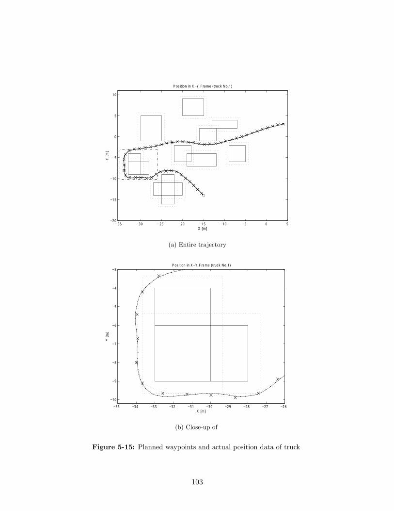
−35 −30 −25 −20 −15 −10 −5 0 5−20

−15

−10

−5

0

5

10

Position in X−Y Frame (truck No.1)

X [m]

Y [m

]

(a) Entire trajectory

−35 −34 −33 −32 −31 −30 −29 −28 −27 −26

−10

−9

−8

−7

−6

−5

−4

−3Position in X−Y Frame (truck No.1)

X [m]

Y [m

]

(b) Close-up of

Figure 5-15: Planned waypoints and actual position data of truck

103

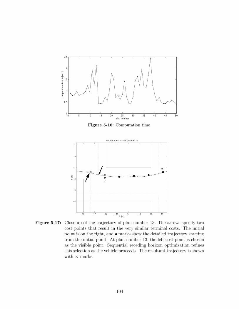
0 5 10 15 20 25 30 35 40 45 500

0.5

1

1.5

2

2.5

plan number

com

puta

tion

time

in [s

ec]

Figure 5-16: Computation time

−18 −17 −16 −15 −14 −13 −12 −11

−4

−3

−2

−1

0

1

Position in X−Y Frame (truck No.1)

X [m]

Y [m

]

x0

xf

Figure 5-17: Close-up of the trajectory of plan number 13. The arrows specify twocost points that result in the very similar terminal costs. The initialpoint is on the right, and • marks show the detailed trajectory startingfrom the initial point. At plan number 13, the left cost point is chosenas the visible point. Sequential receding horizon optimization refinesthis selection as the vehicle proceeds. The resultant trajectory is shownwith × marks.

104

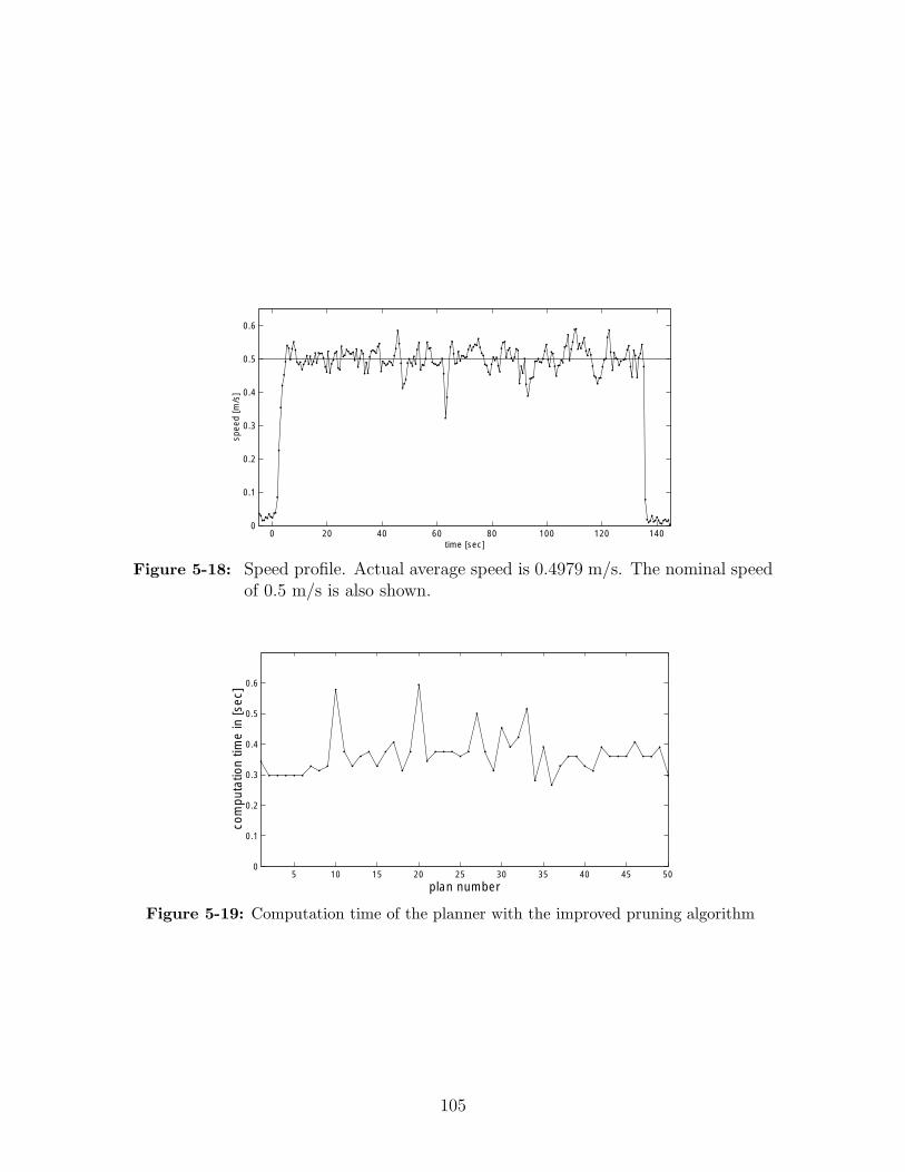
0 20 40 60 80 100 120 1400

0.1

0.2

0.3

0.4

0.5

0.6

spee

d [m

/s]

time [sec]

Figure 5-18: Speed profile. Actual average speed is 0.4979 m/s. The nominal speedof 0.5 m/s is also shown.

5 10 15 20 25 30 35 40 45 500

0.1

0.2

0.3

0.4

0.5

0.6

plan number

com

puta

tion

time

in [s

ec]

Figure 5-19: Computation time of the planner with the improved pruning algorithm

105

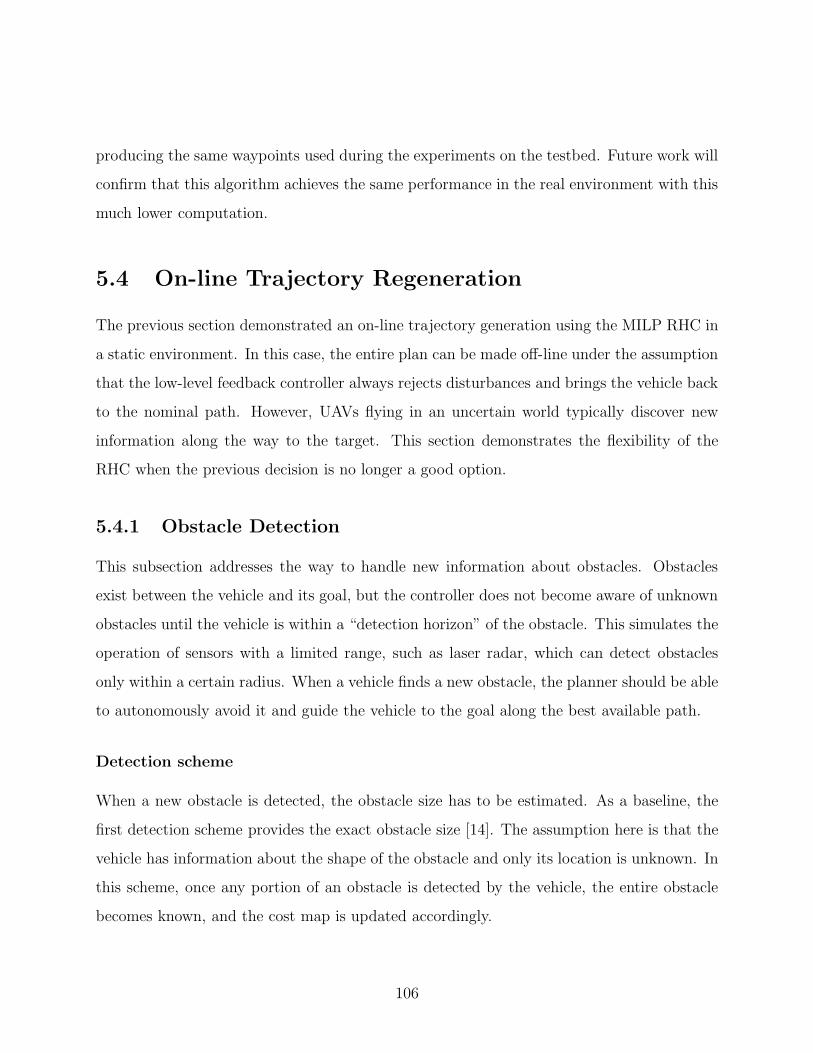
producing the same waypoints used during the experiments on the testbed. Future work will

confirm that this algorithm achieves the same performance in the real environment with this

much lower computation.

5.4 On-line Trajectory Regeneration

The previous section demonstrated an on-line trajectory generation using the MILP RHC in

a static environment. In this case, the entire plan can be made off-line under the assumption

that the low-level feedback controller always rejects disturbances and brings the vehicle back

to the nominal path. However, UAVs flying in an uncertain world typically discover new

information along the way to the target. This section demonstrates the flexibility of the

RHC when the previous decision is no longer a good option.

5.4.1 Obstacle Detection

This subsection addresses the way to handle new information about obstacles. Obstacles

exist between the vehicle and its goal, but the controller does not become aware of unknown

obstacles until the vehicle is within a “detection horizon” of the obstacle. This simulates the

operation of sensors with a limited range, such as laser radar, which can detect obstacles

only within a certain radius. When a vehicle finds a new obstacle, the planner should be able

to autonomously avoid it and guide the vehicle to the goal along the best available path.

Detection scheme

When a new obstacle is detected, the obstacle size has to be estimated. As a baseline, the

first detection scheme provides the exact obstacle size [14]. The assumption here is that the

vehicle has information about the shape of the obstacle and only its location is unknown. In

this scheme, once any portion of an obstacle is detected by the vehicle, the entire obstacle

becomes known, and the cost map is updated accordingly.

106

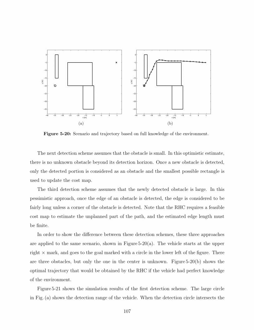
−40 −35 −30 −25 −20 −15 −10 −5 0 5

−35

−30

−25

−20

−15

−10

−5

0

x [m]

y [m

]

1

(a)

−40 −35 −30 −25 −20 −15 −10 −5 0 5

−35

−30

−25

−20

−15

−10

−5

0

x [m]

y [m

]

1

(b)

Figure 5-20: Scenario and trajectory based on full knowledge of the environment.

The next detection scheme assumes that the obstacle is small. In this optimistic estimate,

there is no unknown obstacle beyond its detection horizon. Once a new obstacle is detected,

only the detected portion is considered as an obstacle and the smallest possible rectangle is

used to update the cost map.

The third detection scheme assumes that the newly detected obstacle is large. In this

pessimistic approach, once the edge of an obstacle is detected, the edge is considered to be

fairly long unless a corner of the obstacle is detected. Note that the RHC requires a feasible

cost map to estimate the unplanned part of the path, and the estimated edge length must

be finite.

In order to show the difference between these detection schemes, these three approaches

are applied to the same scenario, shown in Figure 5-20(a). The vehicle starts at the upper

right × mark, and goes to the goal marked with a circle in the lower left of the figure. There

are three obstacles, but only the one in the center is unknown. Figure 5-20(b) shows the

optimal trajectory that would be obtained by the RHC if the vehicle had perfect knowledge

of the environment.

Figure 5-21 shows the simulation results of the first detection scheme. The large circle

in Fig. (a) shows the detection range of the vehicle. When the detection circle intersects the

107

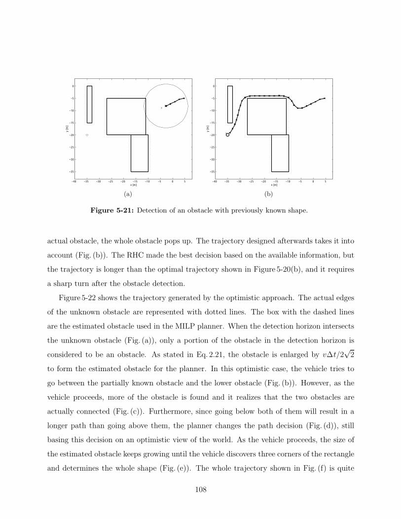
−40 −35 −30 −25 −20 −15 −10 −5 0 5

−35

−30

−25

−20

−15

−10

−5

0

x [m]

y [m

]

(a)

−40 −35 −30 −25 −20 −15 −10 −5 0 5

−35

−30

−25

−20

−15

−10

−5

0

x [m]

y [m

]

1

(b)

Figure 5-21: Detection of an obstacle with previously known shape.

actual obstacle, the whole obstacle pops up. The trajectory designed afterwards takes it into

account (Fig. (b)). The RHC made the best decision based on the available information, but

the trajectory is longer than the optimal trajectory shown in Figure 5-20(b), and it requires

a sharp turn after the obstacle detection.

Figure 5-22 shows the trajectory generated by the optimistic approach. The actual edges

of the unknown obstacle are represented with dotted lines. The box with the dashed lines

are the estimated obstacle used in the MILP planner. When the detection horizon intersects

the unknown obstacle (Fig. (a)), only a portion of the obstacle in the detection horizon is

considered to be an obstacle. As stated in Eq. 2.21, the obstacle is enlarged by v∆t/2√2

to form the estimated obstacle for the planner. In this optimistic case, the vehicle tries to

go between the partially known obstacle and the lower obstacle (Fig. (b)). However, as the

vehicle proceeds, more of the obstacle is found and it realizes that the two obstacles are

actually connected (Fig. (c)). Furthermore, since going below both of them will result in a

longer path than going above them, the planner changes the path decision (Fig. (d)), still

basing this decision on an optimistic view of the world. As the vehicle proceeds, the size of

the estimated obstacle keeps growing until the vehicle discovers three corners of the rectangle

and determines the whole shape (Fig. (e)). The whole trajectory shown in Fig. (f) is quite

108

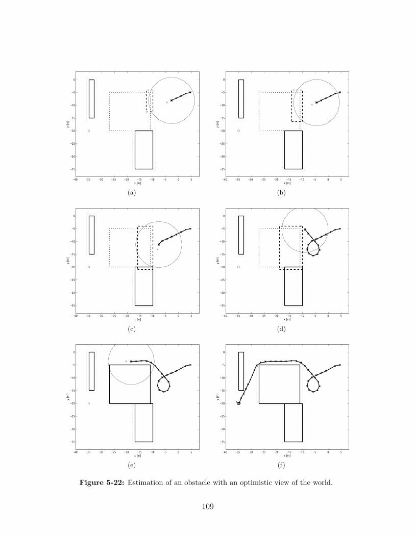
−40 −35 −30 −25 −20 −15 −10 −5 0 5

−35

−30

−25

−20

−15

−10

−5

0

x [m]

y [m

]

(a)

−40 −35 −30 −25 −20 −15 −10 −5 0 5

−35

−30

−25

−20

−15

−10

−5

0

x [m]

y [m

]

(b)

−40 −35 −30 −25 −20 −15 −10 −5 0 5

−35

−30

−25

−20

−15

−10

−5

0

x [m]

y [m

]

(c)

−40 −35 −30 −25 −20 −15 −10 −5 0 5

−35

−30

−25

−20

−15

−10

−5

0

x [m]

y [m

]

(d)

−40 −35 −30 −25 −20 −15 −10 −5 0 5

−35

−30

−25

−20

−15

−10

−5

0

x [m]

y [m

]

(e)

−40 −35 −30 −25 −20 −15 −10 −5 0 5

−35

−30

−25

−20

−15

−10

−5

0

x [m]

y [m

]

1

(f)

Figure 5-22: Estimation of an obstacle with an optimistic view of the world.

109

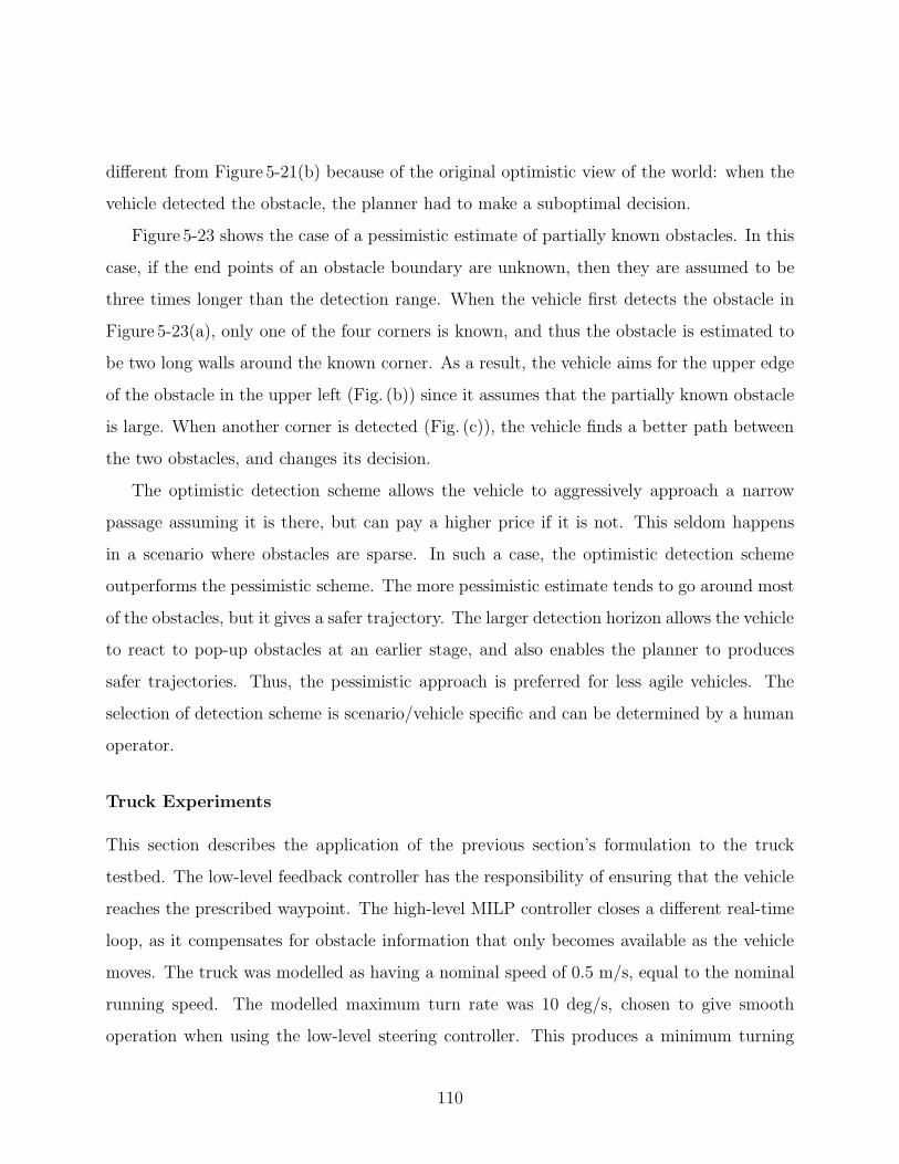
different from Figure 5-21(b) because of the original optimistic view of the world: when the

vehicle detected the obstacle, the planner had to make a suboptimal decision.

Figure 5-23 shows the case of a pessimistic estimate of partially known obstacles. In this

case, if the end points of an obstacle boundary are unknown, then they are assumed to be

three times longer than the detection range. When the vehicle first detects the obstacle in

Figure 5-23(a), only one of the four corners is known, and thus the obstacle is estimated to

be two long walls around the known corner. As a result, the vehicle aims for the upper edge

of the obstacle in the upper left (Fig. (b)) since it assumes that the partially known obstacle

is large. When another corner is detected (Fig. (c)), the vehicle finds a better path between

the two obstacles, and changes its decision.

The optimistic detection scheme allows the vehicle to aggressively approach a narrow

passage assuming it is there, but can pay a higher price if it is not. This seldom happens

in a scenario where obstacles are sparse. In such a case, the optimistic detection scheme

outperforms the pessimistic scheme. The more pessimistic estimate tends to go around most

of the obstacles, but it gives a safer trajectory. The larger detection horizon allows the vehicle

to react to pop-up obstacles at an earlier stage, and also enables the planner to produces

safer trajectories. Thus, the pessimistic approach is preferred for less agile vehicles. The

selection of detection scheme is scenario/vehicle specific and can be determined by a human

operator.

Truck Experiments

This section describes the application of the previous section’s formulation to the truck

testbed. The low-level feedback controller has the responsibility of ensuring that the vehicle

reaches the prescribed waypoint. The high-level MILP controller closes a different real-time

loop, as it compensates for obstacle information that only becomes available as the vehicle

moves. The truck was modelled as having a nominal speed of 0.5 m/s, equal to the nominal

running speed. The modelled maximum turn rate was 10 deg/s, chosen to give smooth

operation when using the low-level steering controller. This produces a minimum turning

110

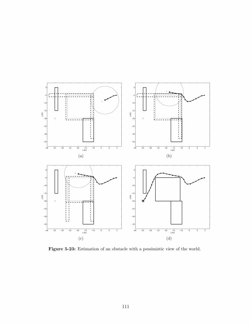
−40 −35 −30 −25 −20 −15 −10 −5 0 5

−35

−30

−25

−20

−15

−10

−5

0

x [m]

y [m

]

(a)

−40 −35 −30 −25 −20 −15 −10 −5 0 5

−35

−30

−25

−20

−15

−10

−5

0

x [m]

y [m

]

(b)

−40 −35 −30 −25 −20 −15 −10 −5 0 5

−35

−30

−25

−20

−15

−10

−5

0

x [m]

y [m

]

(c)

−40 −35 −30 −25 −20 −15 −10 −5 0 5

−35

−30

−25

−20

−15

−10

−5

0

x [m]

y [m

]

1

(d)

Figure 5-23: Estimation of an obstacle with a pessimistic view of the world.

111

radius of 2.8 m. The system was discretized with a time step length of 4 seconds, long

enough for the transient of the low-level steering controller to decay. The planning horizon

was five steps, equivalent to 10 m. The execution horizon was one step: before each plan

was found, only one new waypoint was executed by the truck.

The detection horizon was 9.5 m, which enables the truck to perform collision avoidance

maneuvers once it detects a new obstacle. Initially, the cost map is computed using only

known obstacles and those within the detection horizon of the starting point. At each

step, before the trajectory design phase, the circle around the current position called the

detection horizon is checked for intersections with new obstacles. If any are “found,” the cost

estimation is repeated with the updated obstacle information. This cost estimation process

can be extended to incrementally update the cost map using local information.

In summary, the control scheme is as follows1:

1. If the detection circle intersects any “unknown” part of the obstacles (or if starting),

compute the cost map, including all obstacles currently known.

2. Solve MILP minimizing J in Eq. 2.56 subject to Eqs. 2.2 to 2.57, starting from the last

waypoint uploaded (or initial state if starting).

3. Upload the first ne waypoints of the new plan to the vehicle.

4. Wait until the vehicle reaches the execution horizon of the previous plan.

5. Go to 1.

The optimistic approach of the detection scheme is selected as a test scenario since, with

this approach, the vehicle constantly updates the obstacle information as it gets closer to the

obstacle. The scenario can be seen in Figure 5-24(a). The truck begins at (4.5, 5), heading

in the direction of the goal (−35,−20). Two obstacles marked by the solid black line areinitially known. There is another obstacle, marked by dots, blocking the direct path to the

goal. However, it is not initially known to the planner. To successfully complete the test,

the vehicle must move around the obstacle, once aware of its presence, and reach the goal.

1Compare with the one for a stationary environment (p.101).

112

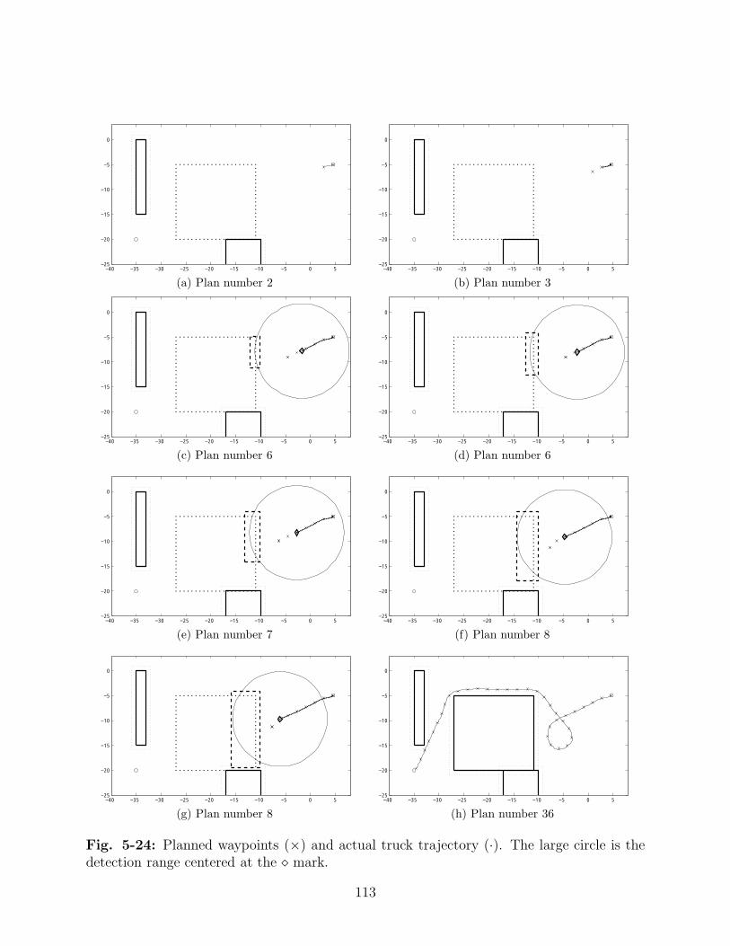
−40 −35 −30 −25 −20 −15 −10 −5 0 5−25

−20

−15

−10

−5

0

(a) Plan number 2−40 −35 −30 −25 −20 −15 −10 −5 0 5

−25

−20

−15

−10

−5

0

(b) Plan number 3

−40 −35 −30 −25 −20 −15 −10 −5 0 5−25

−20

−15

−10

−5

0

(c) Plan number 6−40 −35 −30 −25 −20 −15 −10 −5 0 5

−25

−20

−15

−10

−5

0

(d) Plan number 6

−40 −35 −30 −25 −20 −15 −10 −5 0 5−25

−20

−15

−10

−5

0

(e) Plan number 7−40 −35 −30 −25 −20 −15 −10 −5 0 5

−25

−20

−15

−10

−5

0

(f) Plan number 8

−40 −35 −30 −25 −20 −15 −10 −5 0 5−25

−20

−15

−10

−5

0

(g) Plan number 8−40 −35 −30 −25 −20 −15 −10 −5 0 5

−25

−20

−15

−10

−5

0

(h) Plan number 36

Fig. 5-24: Planned waypoints (×) and actual truck trajectory (·). The large circle is thedetection range centered at the � mark.

113

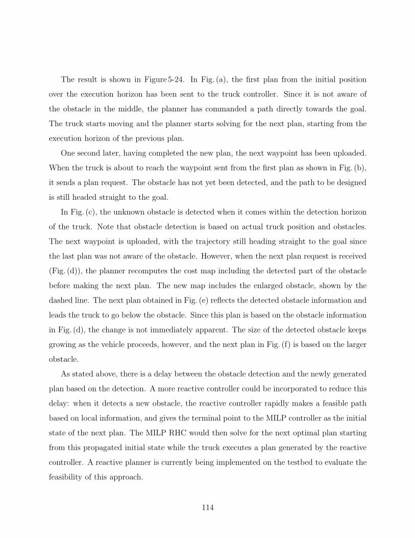
The result is shown in Figure 5-24. In Fig. (a), the first plan from the initial position

over the execution horizon has been sent to the truck controller. Since it is not aware of

the obstacle in the middle, the planner has commanded a path directly towards the goal.

The truck starts moving and the planner starts solving for the next plan, starting from the

execution horizon of the previous plan.

One second later, having completed the new plan, the next waypoint has been uploaded.

When the truck is about to reach the waypoint sent from the first plan as shown in Fig. (b),

it sends a plan request. The obstacle has not yet been detected, and the path to be designed

is still headed straight to the goal.

In Fig. (c), the unknown obstacle is detected when it comes within the detection horizon

of the truck. Note that obstacle detection is based on actual truck position and obstacles.

The next waypoint is uploaded, with the trajectory still heading straight to the goal since

the last plan was not aware of the obstacle. However, when the next plan request is received

(Fig. (d)), the planner recomputes the cost map including the detected part of the obstacle

before making the next plan. The new map includes the enlarged obstacle, shown by the

dashed line. The next plan obtained in Fig. (e) reflects the detected obstacle information and

leads the truck to go below the obstacle. Since this plan is based on the obstacle information

in Fig. (d), the change is not immediately apparent. The size of the detected obstacle keeps

growing as the vehicle proceeds, however, and the next plan in Fig. (f) is based on the larger

obstacle.

As stated above, there is a delay between the obstacle detection and the newly generated

plan based on the detection. A more reactive controller could be incorporated to reduce this

delay: when it detects a new obstacle, the reactive controller rapidly makes a feasible path

based on local information, and gives the terminal point to the MILP controller as the initial

state of the next plan. The MILP RHC would then solve for the next optimal plan starting

from this propagated initial state while the truck executes a plan generated by the reactive

controller. A reactive planner is currently being implemented on the testbed to evaluate the

feasibility of this approach.

114

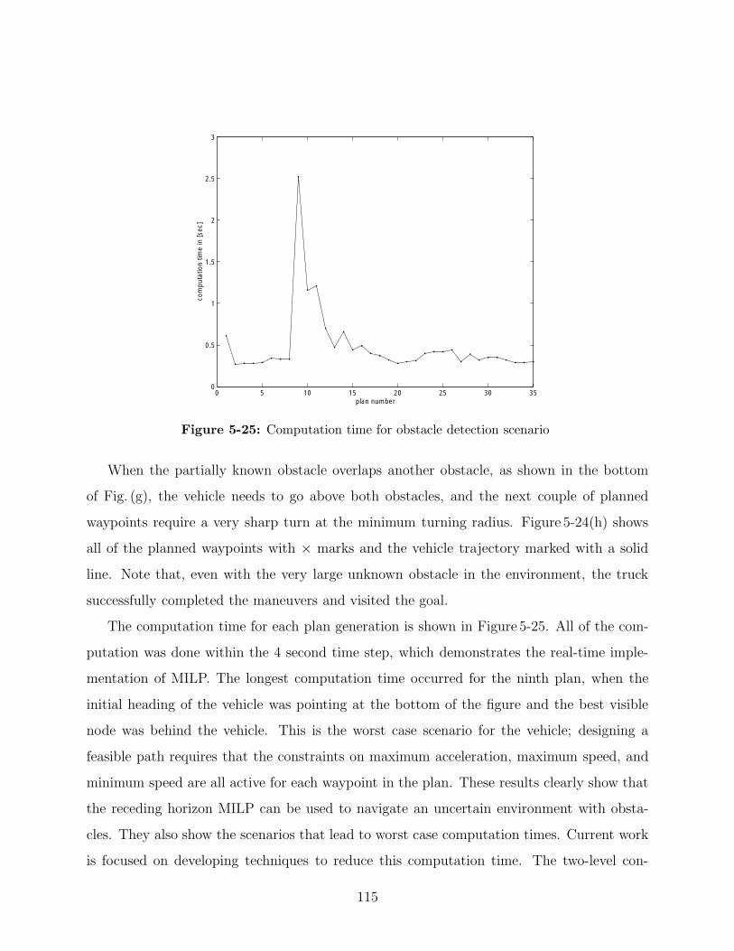
0 5 10 15 20 25 30 350

0.5

1

1.5

2

2.5

3

plan number

com

puta

tion

time

in [s

ec]

Figure 5-25: Computation time for obstacle detection scenario

When the partially known obstacle overlaps another obstacle, as shown in the bottom

of Fig. (g), the vehicle needs to go above both obstacles, and the next couple of planned

waypoints require a very sharp turn at the minimum turning radius. Figure 5-24(h) shows

all of the planned waypoints with × marks and the vehicle trajectory marked with a solid

line. Note that, even with the very large unknown obstacle in the environment, the truck

successfully completed the maneuvers and visited the goal.

The computation time for each plan generation is shown in Figure 5-25. All of the com-

putation was done within the 4 second time step, which demonstrates the real-time imple-

mentation of MILP. The longest computation time occurred for the ninth plan, when the

initial heading of the vehicle was pointing at the bottom of the figure and the best visible

node was behind the vehicle. This is the worst case scenario for the vehicle; designing a

feasible path requires that the constraints on maximum acceleration, maximum speed, and

minimum speed are all active for each waypoint in the plan. These results clearly show that

the receding horizon MILP can be used to navigate an uncertain environment with obsta-

cles. They also show the scenarios that lead to worst case computation times. Current work

is focused on developing techniques to reduce this computation time. The two-level con-

115

trol architecture allows the on-line planner to compensate for obstacle discovery beyond the

execution horizon while low-level feedback rejects vehicle disturbance within that horizon.

5.4.2 Collision Avoidance Maneuver

The control laws for the low-level feedback loops described in Section 5.3 account for the

error in the cross-track direction and the error from the nominal reference speed. Although

the PI speed controller does not have a steady state speed error, it cannot completely nullify

the in-track position error. This in-track error translates into an error in the time-of-arrival

at each waypoint. Failure to meet a timing constraint can cause a significant problem when

coordination of multiple vehicles is required. This subsection demonstrates, using an example

based on a collision avoidance maneuver, that the MILP RHC can re-optimize the trajectory

on-line, accounting for in-track position errors. It also modifies the cost-to-go to improve

the performance of the collision avoidance maneuver.

Cost-To-Go in Relative Frame

In the trajectory design problems for multiple UAVs, the vehicle avoidance constraints be-

come apparent only when the two vehicles come close to each other. This allows us to solve

the trajectory optimization problem without including the full set of vehicle avoidance con-

ditions, which reduces the number of binaries and the computation load. However, when the

planned trajectories for the multiple vehicles intersect with each other, another algorithm is

required that focuses on avoiding collisions.

The cost-to-go method presented in Section 2.4 does not take into account the vehicle

collision avoidance beyond the planning horizon if it is applied to more than one vehicle.

Figure 5-26 shows that this approach can lead to a sub-optimal decision if collision avoidance

is a dominant factor in determining the trajectory. In this example, the two vehicles start

at the right heading towards the left. Their goals are placed such that the two vehicles must

switch their positions in the y direction. Fig. (b) shows the relative positions beginning at

the top of the figure and descending to the goal marked with ◦, where the relative frame for

116

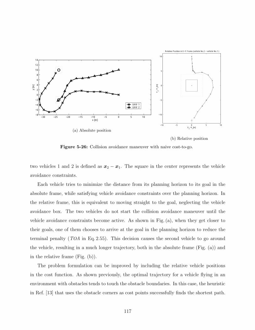
−30 −25 −20 −15 −10 −5 0 5 10−8

−6

−4

−2

0

2

4

6

8

10

12

14

x [m]

y [m

]

UAV 1UAV 2

(a) Absolute position−10 −5 0 5 10

−10

−5

0

5

10

Relative Position in X−Y Frame (vehicle No.2 − vehicle No.1 )

X2−X

1[m]

Y2−

Y1[m

]

(b) Relative position

Figure 5-26: Collision avoidance maneuver with naive cost-to-go.

two vehicles 1 and 2 is defined as x2 − x1. The square in the center represents the vehicle

avoidance constraints.

Each vehicle tries to minimize the distance from its planning horizon to its goal in the

absolute frame, while satisfying vehicle avoidance constraints over the planning horizon. In

the relative frame, this is equivalent to moving straight to the goal, neglecting the vehicle

avoidance box. The two vehicles do not start the collision avoidance maneuver until the

vehicle avoidance constraints become active. As shown in Fig. (a), when they get closer to

their goals, one of them chooses to arrive at the goal in the planning horizon to reduce the

terminal penalty (TOA in Eq. 2.55). This decision causes the second vehicle to go around

the vehicle, resulting in a much longer trajectory, both in the absolute frame (Fig. (a)) and

in the relative frame (Fig. (b)).

The problem formulation can be improved by including the relative vehicle positions

in the cost function. As shown previously, the optimal trajectory for a vehicle flying in an

environment with obstacles tends to touch the obstacle boundaries. In this case, the heuristic

in Ref. [13] that uses the obstacle corners as cost points successfully finds the shortest path.

117

In the vehicle avoidance case, a similar heuristic is that the optimal trajectory will tend to

“follow” the vehicle avoidance box in the relative frame. Therefore, the modified formulation

presented here uses the four corners of the vehicle avoidance box and a relative position of the

two goals as the cost points [xcp,ycp,]T in the relative frame. Eqs. 2.29 to 2.38 in Chapter 2

are replaced with the following equations. For any pair of two vehicles j and k (j < k),

cvis,jk =5∑

i=1

ci bcp,ijk (5.6)

5∑i=1

bcp,ijk = 1 (5.7)

xvis,jk

yvis,jk

= 5∑

i=1

xcp,ijk

ycp,ijk

bcp,ijk (5.8)

xLOS,jk

yLOS,jk

=

xvis,jk

yvis,jk

−

(xnp)k − (xnp)j

(ynp)k − (ynp)j

(5.9)

xtest,jkm

ytest,jkm

=

(xnp)k − (xnp)j

(ynp)k − (ynp)j

+ m

nt

xLOS,jk

yLOS,jk

(5.10)

xtest,jkm ≤ −(dj + dk) +M bvis,1jkm (5.11)

ytest,jkm ≤ −(dj + dk) +M bvis,2jkm (5.12)

xtest,jkm ≥ (dj + dk)−M bvis,3jkm (5.13)

ytest,jkm ≥ (dj + dk)−M bvis,4jkm (5.14)

4∑n=1

bvis,njkm ≤ 3 (5.15)

j = 1, . . . , nv − 1, k = j + 1, . . . , nv, m = 1, . . . , nt

where nt represents a number of test points placed between the planning horizon and the se-

lected cost point to ensure the visibility in the relative frame [14]. Note that xcp,xvis,xLOS,xtest

are in the relative frame whereas xnp is measured in the absolute frame. The cost function

includes, together with the cost-to-go at the selected point, the length of the line-of-sight

vectors in the absolute frame (denoted by li for the ith vehicle) and relative frame (denoted

118

by lrel,jk for a pair of vehicles j and k). Therefore, the objective J2 to be minimized is

J2 =nv∑i=1

li +nv−1∑j=1

nv∑k=j+1

(α lrel,jk + β cvis,jk) (5.16)

li ≥ xgoal,i − (xnp)i

ygoal,i − (ynp)i

im (5.17)

lrel,jk ≥ xLOS,jk

yLOS,jk

im (5.18)

im =

cos

(2πm

nl

)

sin(2πm

nl

) (5.19)

i = 1, . . . , nv, j = 1, . . . , nv − 1, k = j + 1, . . . , nv, m = 1, . . . , nl

where α is a weighting factor for the line-of-sight vector in the relative frame, as defined in

Eq. 5.9, and β is a weighting factor for the cost-to-go at the cost point in the relative frame.

If the goal is not visible from the initial position in the relative frame, (i.e., the paths of the

two vehicles intersect in the absolute frame), the weights α and β navigate the vehicle to

“hug” around the vehicle avoidance box, initiating the collision avoidance action. Larger α

and β navigate the relative position towards the goal faster in the relative frame, but overly

large weights delay the arrival at the goals in the absolute frame because the distances from

the vehicles to their goals have a smaller effect on the objective function.

Note that if there are three vehicles involved, three relative positions (2–1, 3–2, 1–3) must

be accounted for. However, this situation seldom happens because the typical UAVs operate

with a large separation distance compared to their vehicle size.

This formulation is applied to the same scenario presented in Figure 5-26, and the result

is shown in Figure 5-27. In contrast to Figure 5-26(a), vehicle 2 begins a collision avoidance

maneuver immediately. Figure 5-27(b) shows that the relative trajectory successfully avoids

the separation box, with some waypoints falling on the boundary.

119

−30 −25 −20 −15 −10 −5 0 5 10−8

−6

−4

−2

0

2

4

6

8

10

12

14

x [m]

y [m

]

UAV 1UAV 2

(a) Absolute position−10 −5 0 5 10

−10

−5

0

5

10

Relative Position in X−Y Frame (vehicle No.2 − vehicle No.1 )

X2−X

1[m]

Y2−

Y1[m

]

(b) Relative position

Figure 5-27: Collision avoidance maneuver with improved cost-to-go

Truck Experiments

The improved formulation for collision avoidance maneuver is experimentally tested using

two trucks. In the single vehicle case shown in Subsection 5.3.2 and Subsection 5.4.1, a plan

request is sent when the vehicle reaches the execution horizon, and the receding horizon

controller re-optimizes the trajectory before the system reaches the end of the plan. In this

two-truck case, a plan request is sent when either one of the vehicles reaches its horizon point.

The speed controller in this experiment has a low bandwidth, and the MILP RHC controls

the in-track position by adjusting the initial position of each plan, so that the vehicles reach

waypoints at the right time. To see the effect of in-track adjustment by the RHC, three

trials are conducted with different disturbances and control schemes:

Case–1: Small disturbance. No adjustment of in-track position.

Case–2: Small disturbance. Adjustment of in-track position by RHC.

Case–3: Large disturbance. Adjustment of in-track position by RHC.

The following parameters are used:

120

• v∆t = 3.5 [m]• v = 0.5 [m/s]• rmin = 5 [m]

• np = 4• ne = 1• Safety box for each truck: 0.8 [m] × 0.8 [m]

Figure 5-28(a) shows the planned waypoints of the first scenario. The two vehicles start in

the upper right of the figure and go to the lower left while switching their relative positions. In

Figure 5-28(b) and Figure 5-29, × marks represent the planned waypoints, and dots representthe position data reported from the trucks. The relative position starts in the lower right

of Fig. (b) and goes to the upper left. Although the vehicles avoided a collision, the relative

position deviates from the planned trajectory by as much as 1.8 m. This error is mainly

caused by the ground roughness in the test area, which acts as a disturbance to the speed

control loop, resulting in in-track position errors for both vehicles.

One way to improve this situation is to introduce an in-track position control loop in

the low-level feedback controller. This requires the use of the time stamp placed by the

planner at each waypoint. Another approach presented here is to feed the in-track error

back into the receding horizon control loop. Figure 5-30 illustrates this procedure. Let d//

denote the in-track distance to the next waypoint. When d// of either one of the vehicles

becomes smaller than a threshold, the vehicle sends a plan request to the planner. If vehicle

2 is slower than vehicle 1, as is the case in Figure 5-30, the position difference in the in-track

direction (d//)2−(d//)1 is propagated to the initial position of vehicle 2 in the next plan. Thispropagation is accomplished by moving the next initial position backward by (d//)2 − (d//)1.Note that the truck positions are reported at 2 Hz, and an in-track distance d// at a specific

time is obtained through an interpolation.

Figures 5-31 to 5-33 show the result of case–2, where the in-track position is propagated

and fed back to the next initial condition by the RHC. The outcome of the in-track position

adjustment is apparent in Figure 5-31(b) as the discontinuous plans. The lower right of

Figure 5-31(b) is magnified and shown in Figure 5-32 with further explanation. When the

121

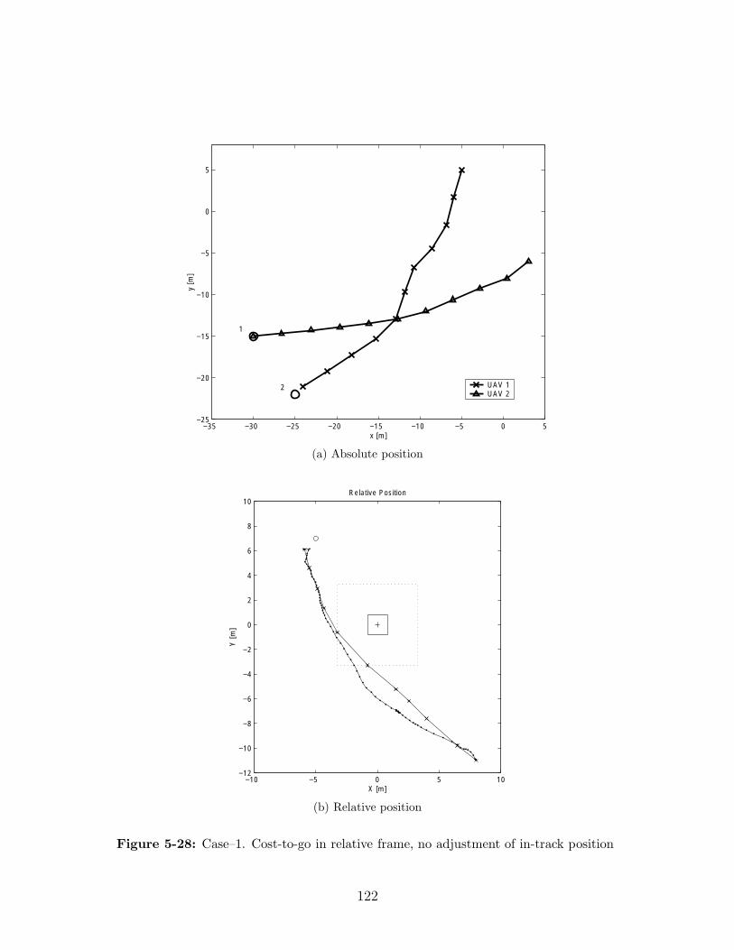
−35 −30 −25 −20 −15 −10 −5 0 5−25

−20

−15

−10

−5

0

5

x [m]

y [m

]

1

2 UAV 1UAV 2

(a) Absolute position

−10 −5 0 5 10−12

−10

−8

−6

−4

−2

0

2

4

6

8

10Relative Position

X [m]

Y [m

]

(b) Relative position

Figure 5-28: Case–1. Cost-to-go in relative frame, no adjustment of in-track position

122

−35 −30 −25 −20 −15 −10 −5 0 5−25

−20

−15

−10

−5

0

5

Position in X−Y Frame (truck No.1)

X [m]

Y [m

]

(a) Truck 1

−35 −30 −25 −20 −15 −10 −5 0 5−25

−20

−15

−10

−5

0

5

Position in X−Y Frame (truck No.2)

X [m]

Y [m

]

(b) Truck 2

Figure 5-29: Case–1. Cost-to-go in relative frame, no adjustment of in-track posi-tion. Actual position data in absolute frame is shown.

123

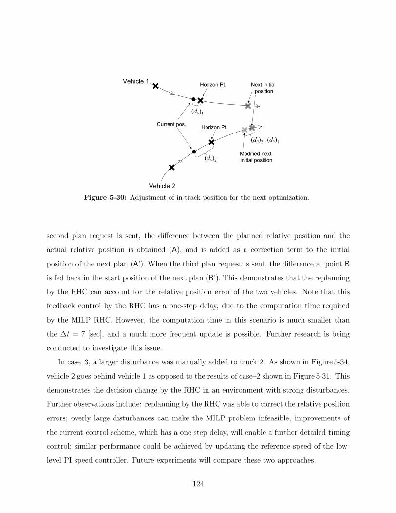
(d//)1

(d//)2

Vehicle 1

Vehicle 2

Horizon Pt.

Horizon Pt.

Next initial

position

Modified next

initial position

Current pos.

(d//)2– (d//)1

Figure 5-30: Adjustment of in-track position for the next optimization.

second plan request is sent, the difference between the planned relative position and the

actual relative position is obtained (A), and is added as a correction term to the initial

position of the next plan (A’). When the third plan request is sent, the difference at point B

is fed back in the start position of the next plan (B’). This demonstrates that the replanning

by the RHC can account for the relative position error of the two vehicles. Note that this

feedback control by the RHC has a one-step delay, due to the computation time required

by the MILP RHC. However, the computation time in this scenario is much smaller than

the ∆t = 7 [sec], and a much more frequent update is possible. Further research is being

conducted to investigate this issue.

In case–3, a larger disturbance was manually added to truck 2. As shown in Figure 5-34,

vehicle 2 goes behind vehicle 1 as opposed to the results of case–2 shown in Figure 5-31. This

demonstrates the decision change by the RHC in an environment with strong disturbances.

Further observations include: replanning by the RHC was able to correct the relative position

errors; overly large disturbances can make the MILP problem infeasible; improvements of

the current control scheme, which has a one step delay, will enable a further detailed timing

control; similar performance could be achieved by updating the reference speed of the low-

level PI speed controller. Future experiments will compare these two approaches.

124

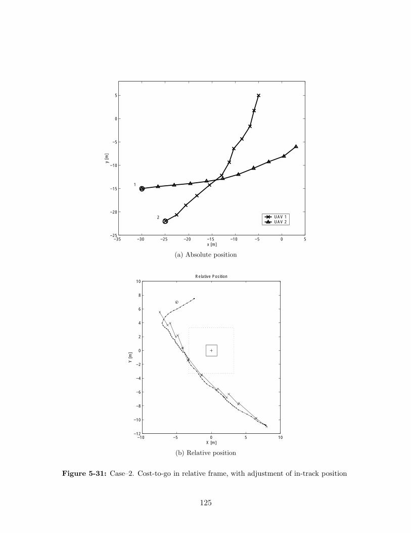
−35 −30 −25 −20 −15 −10 −5 0 5−25

−20

−15

−10

−5

0

5

x [m]

y [m

]

1

2 UAV 1UAV 2

(a) Absolute position

−10 −5 0 5 10−12

−10

−8

−6

−4

−2

0

2

4

6

8

10Relative Position

X [m]

Y [m

]

(b) Relative position

Figure 5-31: Case–2. Cost-to-go in relative frame, with adjustment of in-track position

125

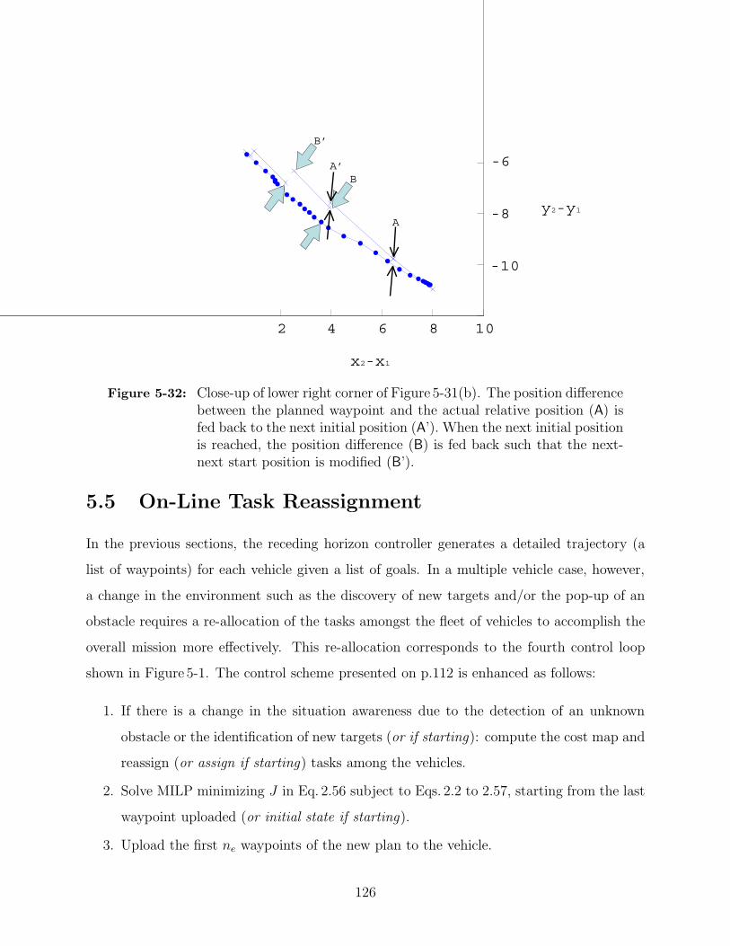
2 4 6 8 10

A

A’

B’

B

-10

-8

-6

x2-x1

y2-y1

Figure 5-32: Close-up of lower right corner of Figure 5-31(b). The position differencebetween the planned waypoint and the actual relative position (A) isfed back to the next initial position (A’). When the next initial positionis reached, the position difference (B) is fed back such that the next-next start position is modified (B’).

5.5 On-Line Task Reassignment

In the previous sections, the receding horizon controller generates a detailed trajectory (a

list of waypoints) for each vehicle given a list of goals. In a multiple vehicle case, however,

a change in the environment such as the discovery of new targets and/or the pop-up of an

obstacle requires a re-allocation of the tasks amongst the fleet of vehicles to accomplish the

overall mission more effectively. This re-allocation corresponds to the fourth control loop

shown in Figure 5-1. The control scheme presented on p.112 is enhanced as follows:

1. If there is a change in the situation awareness due to the detection of an unknown

obstacle or the identification of new targets (or if starting): compute the cost map and

reassign (or assign if starting) tasks among the vehicles.

2. Solve MILP minimizing J in Eq. 2.56 subject to Eqs. 2.2 to 2.57, starting from the last

waypoint uploaded (or initial state if starting).

3. Upload the first ne waypoints of the new plan to the vehicle.

126

−35 −30 −25 −20 −15 −10 −5 0 5−25

−20

−15

−10

−5

0

5

Position in X−Y Frame (truck No.1)

X [m]

Y [m

]

(a) Vehicle 1

−35 −30 −25 −20 −15 −10 −5 0 5−25

−20

−15

−10

−5

0

5

Position in X−Y Frame (truck No.2)

X [m]

Y [m

]

(b) Vehicle 2

Figure 5-33: Case–2. Cost-to-go in relative frame, with adjustment of in-track po-sition. Actual position data in absolute frame is shown.

127

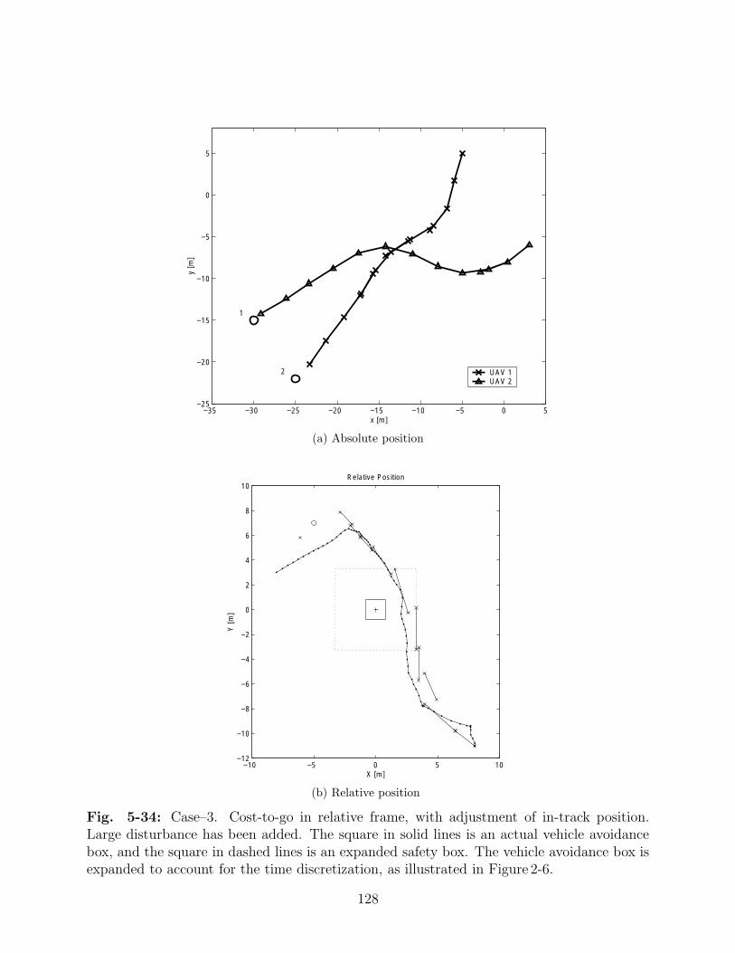
−35 −30 −25 −20 −15 −10 −5 0 5−25

−20

−15

−10

−5

0

5

x [m]

y [m

]

1

2 UAV 1UAV 2

(a) Absolute position

−10 −5 0 5 10−12

−10

−8

−6

−4

−2

0

2

4

6

8

10Relative Position

X [m]

Y [m

]

(b) Relative position

Fig. 5-34: Case–3. Cost-to-go in relative frame, with adjustment of in-track position.Large disturbance has been added. The square in solid lines is an actual vehicle avoidancebox, and the square in dashed lines is an expanded safety box. The vehicle avoidance box isexpanded to account for the time discretization, as illustrated in Figure 2-6.

128

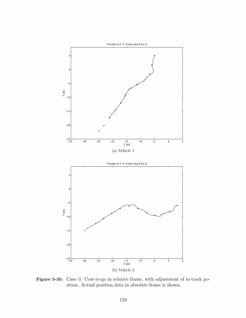
−35 −30 −25 −20 −15 −10 −5 0 5−25

−20

−15

−10

−5

0

5

Position in X−Y Frame (truck No.1)

X [m]

Y [m

]

(a) Vehicle 1

−35 −30 −25 −20 −15 −10 −5 0 5−25

−20

−15

−10

−5

0

5

Position in X−Y Frame (truck No.2)

X [m]

Y [m

]

(b) Vehicle 2

Figure 5-35: Case–3. Cost-to-go in relative frame, with adjustment of in-track po-sition. Actual position data in absolute frame is shown.

129

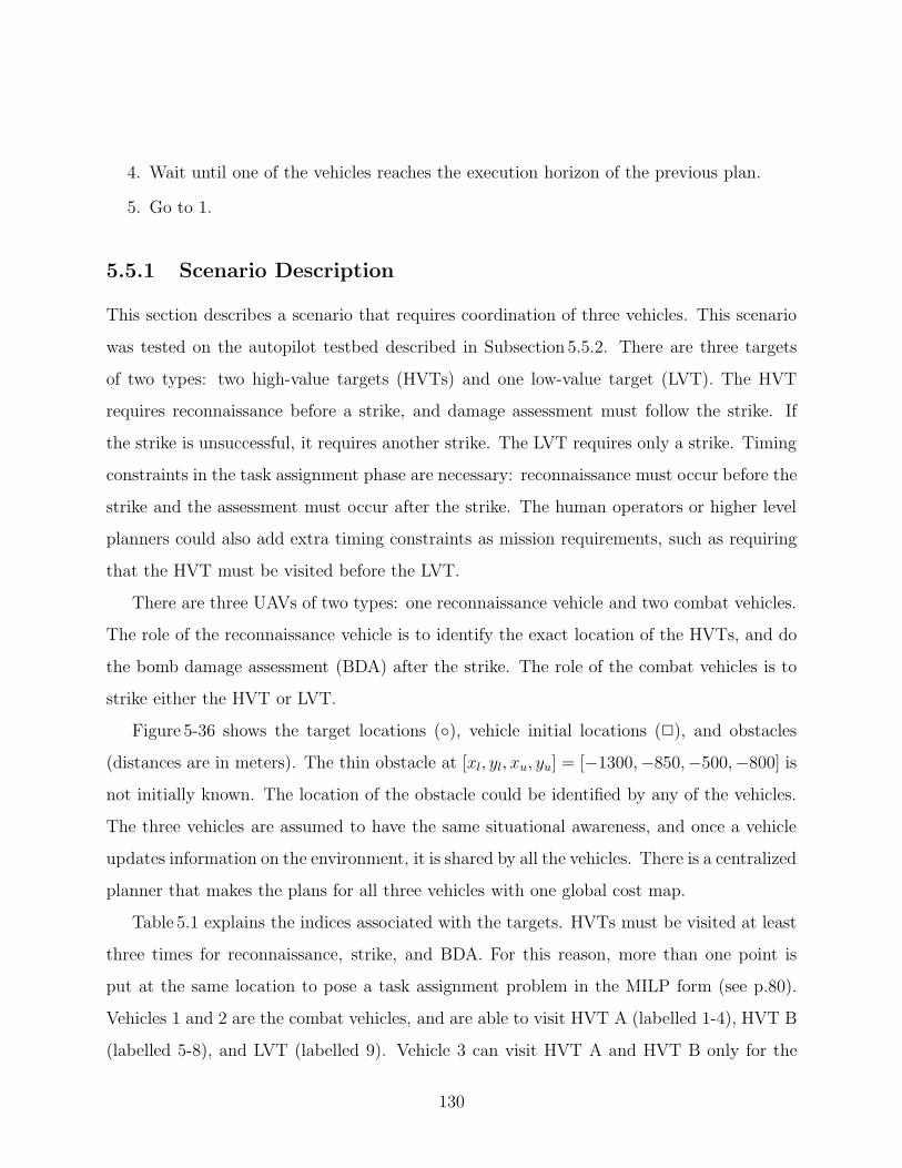
4. Wait until one of the vehicles reaches the execution horizon of the previous plan.

5. Go to 1.

5.5.1 Scenario Description

This section describes a scenario that requires coordination of three vehicles. This scenario

was tested on the autopilot testbed described in Subsection 5.5.2. There are three targets

of two types: two high-value targets (HVTs) and one low-value target (LVT). The HVT

requires reconnaissance before a strike, and damage assessment must follow the strike. If

the strike is unsuccessful, it requires another strike. The LVT requires only a strike. Timing

constraints in the task assignment phase are necessary: reconnaissance must occur before the

strike and the assessment must occur after the strike. The human operators or higher level

planners could also add extra timing constraints as mission requirements, such as requiring

that the HVT must be visited before the LVT.

There are three UAVs of two types: one reconnaissance vehicle and two combat vehicles.

The role of the reconnaissance vehicle is to identify the exact location of the HVTs, and do

the bomb damage assessment (BDA) after the strike. The role of the combat vehicles is to

strike either the HVT or LVT.

Figure 5-36 shows the target locations (◦), vehicle initial locations (✷), and obstacles(distances are in meters). The thin obstacle at [xl, yl, xu, yu] = [−1300,−850,−500,−800] isnot initially known. The location of the obstacle could be identified by any of the vehicles.

The three vehicles are assumed to have the same situational awareness, and once a vehicle

updates information on the environment, it is shared by all the vehicles. There is a centralized

planner that makes the plans for all three vehicles with one global cost map.

Table 5.1 explains the indices associated with the targets. HVTs must be visited at least

three times for reconnaissance, strike, and BDA. For this reason, more than one point is

put at the same location to pose a task assignment problem in the MILP form (see p.80).

Vehicles 1 and 2 are the combat vehicles, and are able to visit HVT A (labelled 1-4), HVT B

(labelled 5-8), and LVT (labelled 9). Vehicle 3 can visit HVT A and HVT B only for the

130

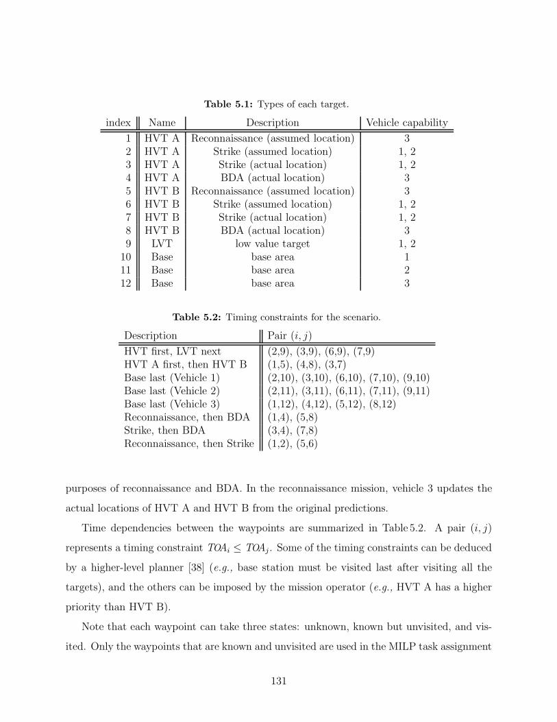
Table 5.1: Types of each target.

index Name Description Vehicle capability

1 HVT A Reconnaissance (assumed location) 32 HVT A Strike (assumed location) 1, 23 HVT A Strike (actual location) 1, 24 HVT A BDA (actual location) 35 HVT B Reconnaissance (assumed location) 36 HVT B Strike (assumed location) 1, 27 HVT B Strike (actual location) 1, 28 HVT B BDA (actual location) 39 LVT low value target 1, 210 Base base area 111 Base base area 212 Base base area 3

Table 5.2: Timing constraints for the scenario.

Description Pair (i, j)

HVT first, LVT next (2,9), (3,9), (6,9), (7,9)HVT A first, then HVT B (1,5), (4,8), (3,7)Base last (Vehicle 1) (2,10), (3,10), (6,10), (7,10), (9,10)Base last (Vehicle 2) (2,11), (3,11), (6,11), (7,11), (9,11)Base last (Vehicle 3) (1,12), (4,12), (5,12), (8,12)Reconnaissance, then BDA (1,4), (5,8)Strike, then BDA (3,4), (7,8)Reconnaissance, then Strike (1,2), (5,6)

purposes of reconnaissance and BDA. In the reconnaissance mission, vehicle 3 updates the

actual locations of HVT A and HVT B from the original predictions.

Time dependencies between the waypoints are summarized in Table 5.2. A pair (i, j)

represents a timing constraint TOAi ≤ TOAj . Some of the timing constraints can be deduced

by a higher-level planner [38] (e.g., base station must be visited last after visiting all the

targets), and the others can be imposed by the mission operator (e.g., HVT A has a higher

priority than HVT B).

Note that each waypoint can take three states: unknown, known but unvisited, and vis-

ited. Only the waypoints that are known and unvisited are used in the MILP task assignment

131

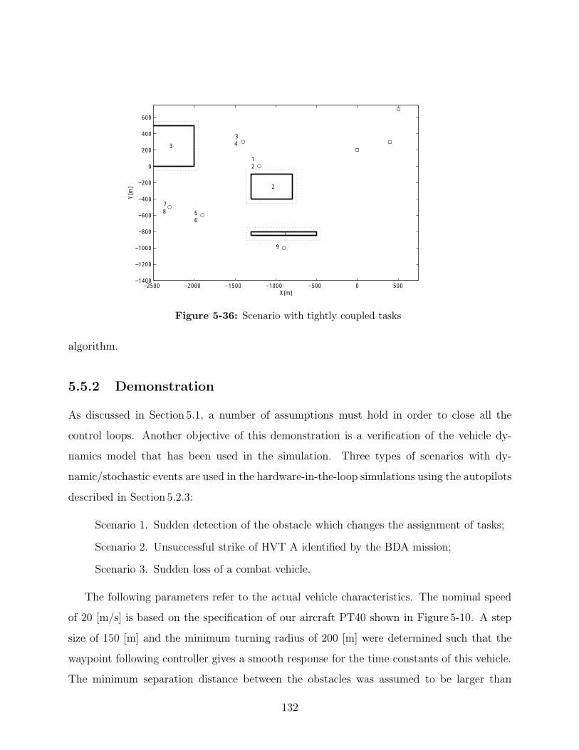
−2500 −2000 −1500 −1000 −500 0 500−1400

−1200

−1000

−800

−600

−400

−200

0

200

400

600

12

34

56

78

9

1

2

3

X[m]

Y[m

]

Figure 5-36: Scenario with tightly coupled tasks

algorithm.

5.5.2 Demonstration

As discussed in Section 5.1, a number of assumptions must hold in order to close all the

control loops. Another objective of this demonstration is a verification of the vehicle dy-

namics model that has been used in the simulation. Three types of scenarios with dy-

namic/stochastic events are used in the hardware-in-the-loop simulations using the autopilots

described in Section 5.2.3:

Scenario 1. Sudden detection of the obstacle which changes the assignment of tasks;

Scenario 2. Unsuccessful strike of HVT A identified by the BDA mission;

Scenario 3. Sudden loss of a combat vehicle.

The following parameters refer to the actual vehicle characteristics. The nominal speed

of 20 [m/s] is based on the specification of our aircraft PT40 shown in Figure 5-10. A step

size of 150 [m] and the minimum turning radius of 200 [m] were determined such that the

waypoint following controller gives a smooth response for the time constants of this vehicle.

The minimum separation distance between the obstacles was assumed to be larger than

132

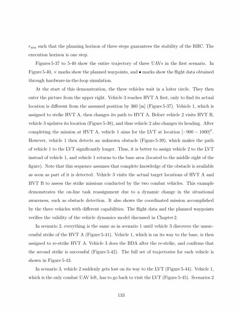
rmin such that the planning horizon of three steps guarantees the stability of the RHC. The

execution horizon is one step.

Figures 5-37 to 5-40 show the entire trajectory of three UAVs in the first scenario. In

Figure 5-40, × marks show the planned waypoints, and •marks show the flight data obtainedthrough hardware-in-the-loop simulation.

At the start of this demonstration, the three vehicles wait in a loiter circle. They then

enter the picture from the upper right. Vehicle 3 reaches HVT A first, only to find its actual

location is different from the assumed position by 360 [m] (Figure 5-37). Vehicle 1, which is

assigned to strike HVT A, then changes its path to HVT A. Before vehicle 2 visits HVT B,

vehicle 3 updates its location (Figure 5-38), and thus vehicle 2 also changes its heading. After

completing the mission at HVT A, vehicle 1 aims for the LVT at location [−900 − 1000]T .However, vehicle 1 then detects an unknown obstacle (Figure 5-39), which makes the path

of vehicle 1 to the LVT significantly longer. Thus, it is better to assign vehicle 2 to the LVT

instead of vehicle 1, and vehicle 1 returns to the base area (located to the middle right of the

figure). Note that this sequence assumes that complete knowledge of the obstacle is available

as soon as part of it is detected. Vehicle 3 visits the actual target locations of HVT A and

HVT B to assess the strike missions conducted by the two combat vehicles. This example

demonstrates the on-line task reassignment due to a dynamic change in the situational

awareness, such as obstacle detection. It also shows the coordinated mission accomplished

by the three vehicles with different capabilities. The flight data and the planned waypoints

verifies the validity of the vehicle dynamics model discussed in Chapter 2.

In scenario 2, everything is the same as in scenario 1 until vehicle 3 discovers the unsuc-

cessful strike of the HVT A (Figure 5-41). Vehicle 1, which is on its way to the base, is then

assigned to re-strike HVT A. Vehicle 3 does the BDA after the re-strike, and confirms that

the second strike is successful (Figure 5-42). The full set of trajectories for each vehicle is

shown in Figure 5-43.

In scenario 3, vehicle 2 suddenly gets lost on its way to the LVT (Figure 5-44). Vehicle 1,

which is the only combat UAV left, has to go back to visit the LVT (Figure 5-45). Scenarios 2

133

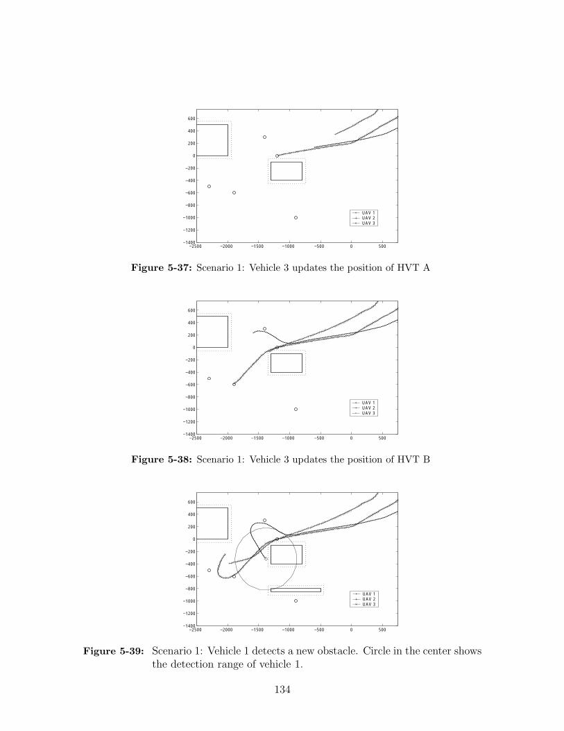
−2500 −2000 −1500 −1000 −500 0 500−1400

−1200

−1000

−800

−600

−400

−200

0

200

400

600

UAV 1UAV 2UAV 3

Figure 5-37: Scenario 1: Vehicle 3 updates the position of HVT A

−2500 −2000 −1500 −1000 −500 0 500−1400

−1200

−1000

−800

−600

−400

−200

0

200

400

600

UAV 1UAV 2UAV 3

Figure 5-38: Scenario 1: Vehicle 3 updates the position of HVT B

−2500 −2000 −1500 −1000 −500 0 500−1400

−1200

−1000

−800

−600

−400

−200

0

200

400

600

UAV 1UAV 2UAV 3

Figure 5-39: Scenario 1: Vehicle 1 detects a new obstacle. Circle in the center showsthe detection range of vehicle 1.

134

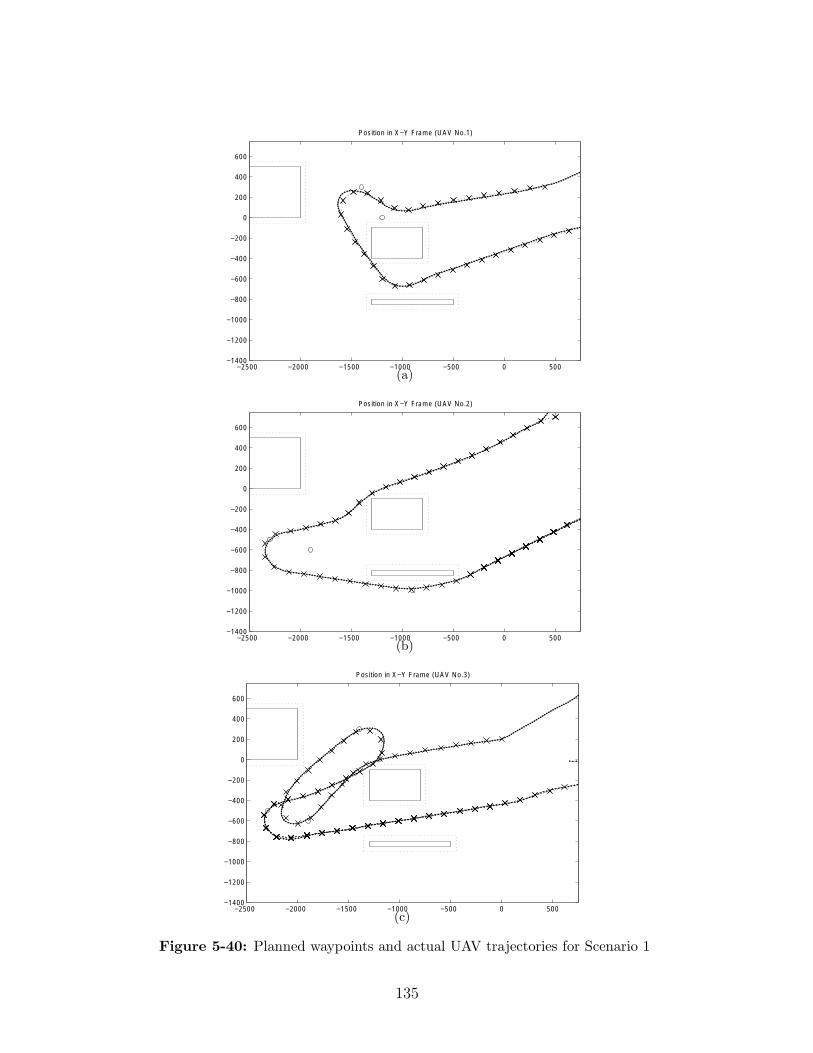
−2500 −2000 −1500 −1000 −500 0 500−1400

−1200

−1000

−800

−600

−400

−200

0

200

400

600

Position in X−Y Frame (UAV No.1)

(a)

−2500 −2000 −1500 −1000 −500 0 500−1400

−1200

−1000

−800

−600

−400

−200

0

200

400

600

Position in X−Y Frame (UAV No.2)

(b)

−2500 −2000 −1500 −1000 −500 0 500−1400

−1200

−1000

−800

−600

−400

−200

0

200

400

600

Position in X−Y Frame (UAV No.3)

(c)

Figure 5-40: Planned waypoints and actual UAV trajectories for Scenario 1

135

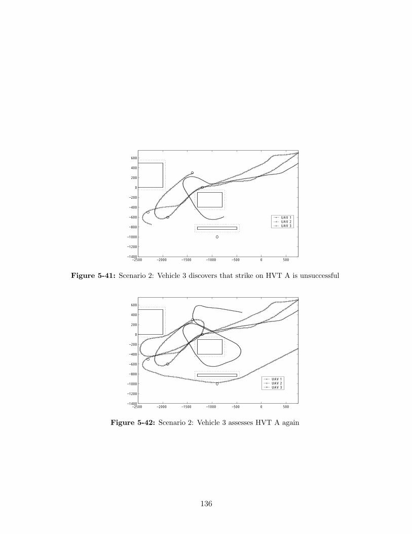
−2500 −2000 −1500 −1000 −500 0 500−1400

−1200

−1000

−800

−600

−400

−200

0

200

400

600

UAV 1UAV 2UAV 3

Figure 5-41: Scenario 2: Vehicle 3 discovers that strike on HVT A is unsuccessful

−2500 −2000 −1500 −1000 −500 0 500−1400

−1200

−1000

−800

−600

−400

−200

0

200

400

600

UAV 1UAV 2UAV 3

Figure 5-42: Scenario 2: Vehicle 3 assesses HVT A again

136

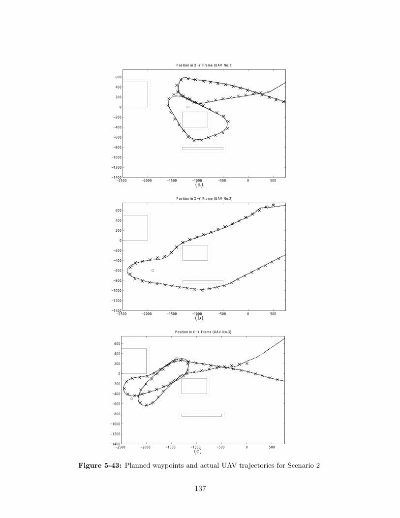
−2500 −2000 −1500 −1000 −500 0 500−1400

−1200

−1000

−800

−600

−400

−200

0

200

400

600

Position in X−Y Frame (UAV No.1)

(a)

−2500 −2000 −1500 −1000 −500 0 500−1400

−1200

−1000

−800

−600

−400

−200

0

200

400

600

Position in X−Y Frame (UAV No.2)

(b)

−2500 −2000 −1500 −1000 −500 0 500−1400

−1200

−1000

−800

−600

−400

−200

0

200

400

600

Position in X−Y Frame (UAV No.3)

(c)

Figure 5-43: Planned waypoints and actual UAV trajectories for Scenario 2

137

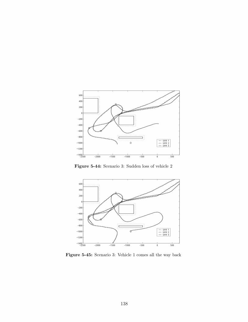
−2500 −2000 −1500 −1000 −500 0 500−1400

−1200

−1000

−800

−600

−400

−200

0

200

400

600

UAV 1UAV 2UAV 3

Figure 5-44: Scenario 3: Sudden loss of vehicle 2

−2500 −2000 −1500 −1000 −500 0 500−1400

−1200

−1000

−800

−600

−400

−200

0

200

400

600

UAV 1UAV 2UAV 3

Figure 5-45: Scenario 3: Vehicle 1 comes all the way back

138

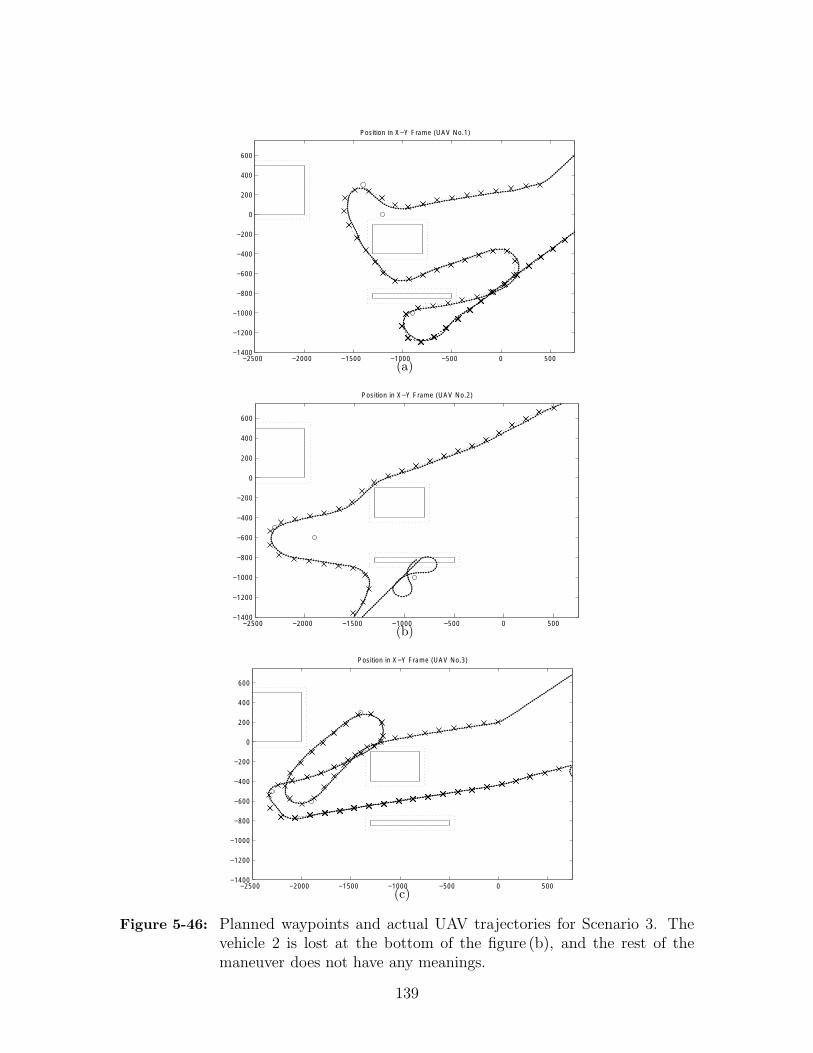
−2500 −2000 −1500 −1000 −500 0 500−1400

−1200

−1000

−800

−600

−400

−200

0

200

400

600

Position in X−Y Frame (UAV No.1)

(a)

−2500 −2000 −1500 −1000 −500 0 500−1400

−1200

−1000

−800

−600

−400

−200

0

200

400

600

Position in X−Y Frame (UAV No.2)

(b)

−2500 −2000 −1500 −1000 −500 0 500−1400

−1200

−1000

−800

−600

−400

−200

0

200

400

600

Position in X−Y Frame (UAV No.3)

(c)

Figure 5-46: Planned waypoints and actual UAV trajectories for Scenario 3. Thevehicle 2 is lost at the bottom of the figure (b), and the rest of themaneuver does not have any meanings.

139

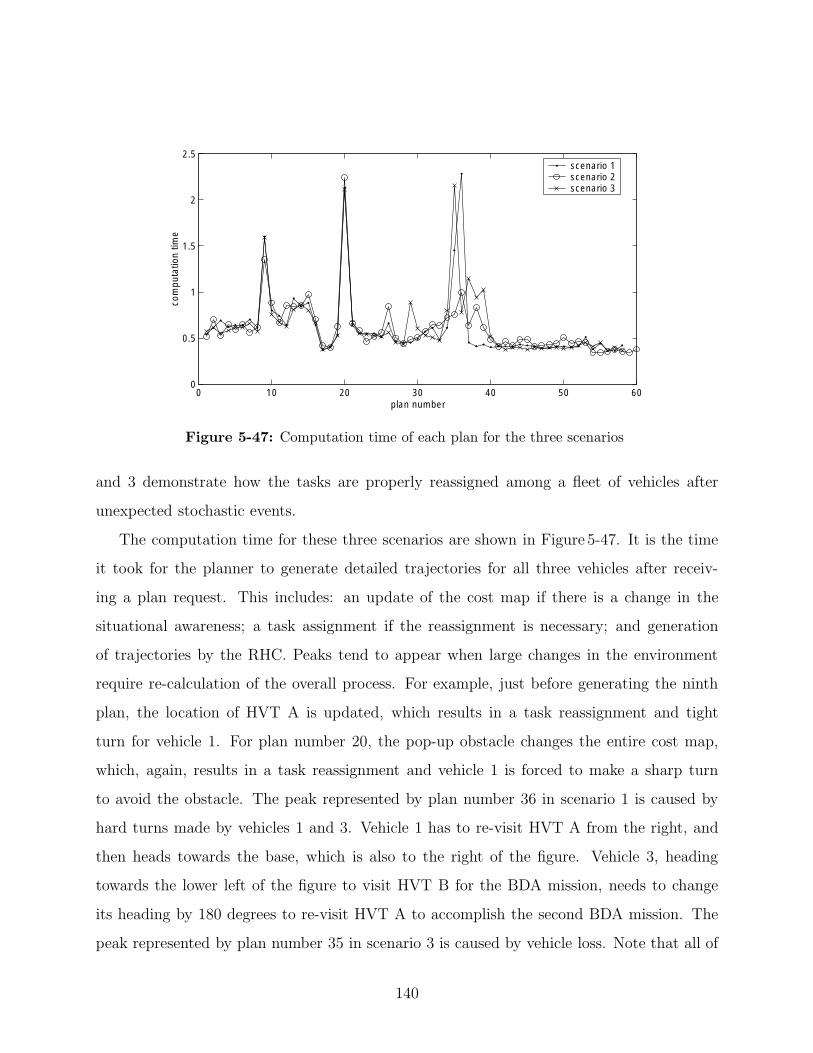
0 10 20 30 40 50 600

0.5

1

1.5

2

2.5

plan number

com

puta

tion

time

scenario 1scenario 2scenario 3

Figure 5-47: Computation time of each plan for the three scenarios

and 3 demonstrate how the tasks are properly reassigned among a fleet of vehicles after

unexpected stochastic events.

The computation time for these three scenarios are shown in Figure 5-47. It is the time

it took for the planner to generate detailed trajectories for all three vehicles after receiv-

ing a plan request. This includes: an update of the cost map if there is a change in the

situational awareness; a task assignment if the reassignment is necessary; and generation

of trajectories by the RHC. Peaks tend to appear when large changes in the environment

require re-calculation of the overall process. For example, just before generating the ninth

plan, the location of HVT A is updated, which results in a task reassignment and tight

turn for vehicle 1. For plan number 20, the pop-up obstacle changes the entire cost map,

which, again, results in a task reassignment and vehicle 1 is forced to make a sharp turn

to avoid the obstacle. The peak represented by plan number 36 in scenario 1 is caused by

hard turns made by vehicles 1 and 3. Vehicle 1 has to re-visit HVT A from the right, and

then heads towards the base, which is also to the right of the figure. Vehicle 3, heading

towards the lower left of the figure to visit HVT B for the BDA mission, needs to change

its heading by 180 degrees to re-visit HVT A to accomplish the second BDA mission. The

peak represented by plan number 35 in scenario 3 is caused by vehicle loss. Note that all of

140

the computation times are well below the discrete time step of ne∆t = 7.5 [sec], and that

the real-time trajectory generation for a fleet of vehicles in these three different scenarios is

successful.

5.6 Conclusions

Several experiments have have been presented to demonstrate the use of MILP for on-line

replanning to control vehicles in the presence of dynamic uncertainties. Four different levels

of control loops have been implemented on a ground vehicle testbed and a UAV hardware-

in-the-loop simulator testbed to demonstrate technologies developed for future UAV control.

The first example validated the on-line trajectory generation using the RHC. This architec-

ture uses MILP for high-level path-planning, while a low-level feedback loop onboard the

vehicle tracks the desired waypoints and rejects disturbances. In one example, a receding

horizon formulation successfully maneuvered a vehicle to its assigned goal with a restricted

detection of obstacles, representing a limited-range radar. In the collision avoidance ma-

neuver, the high-level RHC path planner can account for differences in the time-of-arrival

between two vehicles. The approach uses a feedback correction in the RHC with a one time-

step delay, and on-going research is investigating more reactive techniques. The last example

showed the tight coordination of a fleet of three autonomous vehicles. It also demonstrated

the task re-assignment due to the dynamic and/or stochastic events coupled with a re-design

of trajectory. A faster task re-assignment algorithm will be required when more tasks are

being assigned to larger fleets.

141

142

Chapter 6

Conclusions and Future Work

6.1 Contributions

This thesis presented a real-time trajectory generation method using a receding horizon

control and demonstrated its hardware implementation on two different types of testbeds.

In particular, the following list shows the primary contributions of this thesis:

• Rigorous formulation of the MILP receding horizon trajectory optimization problemthat includes multiple vehicles and multiple goal scenarios.

• An improved formulation of the stable receding horizon controller that guarantees finitetime completion of the mission in a constrained environment.

• Reduction of the computation time of the MILP RHC using a new pruning algorithm.• Extension of the task allocation problem to scenarios with highly coupled tasks and

relative timing constraints.

• Integration of the control algorithms acting on four different levels of the hierarchy inFigure 1-1.

• Demonstration of these planning algorithms in a real environment with disturbances,communication delays, and finite computational power.

Chapter 2 presented the complete receding horizon trajectory design problem in the MILP

form. The binary variables in MILP express the logical constraints such as the goal selection,

143

the path selection, and the collision avoidance. This formulation allows for longer missions

with several tasks because the trajectory is continually generated over a limited range into

the future (i.e., the planning horizon).

The discussion in Chapter 3 bridged the gap between the two models used in the RHC: the

coarse model using the straight line approximation and the detailed model using the point

mass vehicle dynamics. By considering the turning circles at the cost estimation phase,

the path planned based on the straight lines guarantees the existence of a feasible solution

during the MILP trajectory optimization phase. The node elimination and the modified

Dijkstra’s algorithm presented in this chapter allow “unstable” nodes to be pruned without

losing the key candidate options for the optimal path. This pruning also significantly reduces

the computation time.

Chapter 4 presented a task assignment algorithm that can be applied to complicated

scenarios with various time dependencies. Adding the option of loitering as an extra degree

of freedom enables the MILP to find an optimal solution to sophisticated missions, involving

simultaneous arrivals or ordered tasks.

In Chapter 5, the planning algorithms have been demonstrated on two different types of

testbeds. In the real world, disturbances act on the vehicle and its behavior can be different

from what is planned. In an uncertain environment, a change in the situational awareness

might make the existing plan obsolete, and the result of a stochastic event might require

a change in the entire approach to the mission. Chapter 5 demonstrated that replanning

at the various levels of the control hierarchy can be used to compensate for these different

types of uncertainties. Several experiments were conducted to demonstrate the real-time

control loop closures. These included the low-level feedback control, the graph-based path

planning, the MILP based RHC trajectory generation, and the task reassignment among

three heterogeneous vehicles. The experimental results showed that closing the various

loops led to successful mission completion despite the action of disturbances. In addition, the

experimental results indicate that the various assumptions made in the planning/simulations

were valid.

144

6.2 Future Research Directions

While the scenarios examined in this thesis demonstrated the real-time trajectory generation

for reasonably sized problems, a further increase in the size of the problem will lead to a

computational issue for MILP or other non-convex optimization techniques. The computa-

tional issue mainly consists of the following three parts, and further future research will be

required to develop algorithms to overcome them.

First, the problem size increases as the number of vehicles increases. The centralized

planner presented in this thesis will eventually be unable to handle an overly large problem.

However, the MILP trajectory design optimization can be conducted separately for each

vehicle, as mentioned in Chapter 2, if the inter-vehicle collision is not an issue. This motivates

implementing the trajectory design in a distributed architecture, and then using the pair-wise

collision avoidance in Subsection 5.4.2 to avoid collisions.

Second, as the number of obstacles increases, the number of binary variables also in-

creases, which leads to a rapid growth in the computation time. As discussed in Chapter 3, a

pruning algorithm before the MILP optimization phase can significantly reduce the possible

options while keeping the primary candidates for the best solution. Further improvement

in the lower bound of the planning horizon might be possible, which reduces an area where

detailed trajectory needs to be designed.

Third, on-line task reassignment has a large impact on the rate of the planning loop,

as shown in Section 5.5. The computational demands of the task allocation are known to

increase when additional or highly complicated tasks must be allocated. It is very difficult

to solve large allocation problems using the exact or approximate decomposition methods

using MILP. However, heuristic algorithms such as Tabu search [39] provide good solutions

in a reasonable computation time for large problems. Using heuristics to predict the far

future while solving the exact allocation problem in the near term using MILP should also

enable task assignment in a receding horizon fashion.

Overall, the MILP RHC plays an important role in real-time trajectory generation and

execution. In order to enhance the variety and flexibility of mission goals, however, tighter

145

integration with other algorithms such as temporal planning, low-observability technology,

and stochastic programming needs to be explored.

146

Bibliography

[1] P. R. Chandler, M. Pachter, D. Swaroop, J. M. Fowler, J. K. Howlett, S. Rasmussen,

C. Schumacher, and K. Nygard, “Complexity in UAV Cooperative Control,” in Pro-

ceedings of the American Control Conference, (Anchorage AK), May 2002.

[2] C. Schumacher, P. R. Chandler, and S. Rasmussen, “Task Allocation for Wide Area

Search Munitions via Network Flow Optimization,” in Proceedings of the American

Control Conference, (Anchorage AK), pp. 1917–1922, May 2002.

[3] J. Bellingham, M. Tillerson, A. Richards, and J. How, “Multi-Task Allocation and Path

Planning for Cooperating UAVs,” in Second Annual Conference on Cooperative Control

and Optimization, Nov 2001.

[4] A. Richards, J. Bellingham, M. Tillerson, and J. How, “Coordination and Control of

Multiple UAVs,” in Proceedings of the AIAA Guidance, Navigation and Control Con-

ference, (Monterey, CA), Aug 2002.

[5] J. C. Latombe, Robot Motion Planning. Kluwer Academic, 1991.

[6] P. R. Chandler and M. Pachter, “Research Issues in Autonomous Control of Tactical

UAVs,” in Proceedings of the American Control Conference, (Washington, DC), pp. 394–

398, 1998.

[7] A. G. Richards, “Trajectory Optimization using Mixed-Integer Linear Programming,”

Master’s thesis, Massachusetts Institute of Technology, June 2002.

147

[8] A. Richards, T. Schouwenaars, J. How, and E. Feron, “Spacecraft Trajectory Plan-

ning With Collision and Plume Avoidance Using Mixed-Integer Linear Programming,”

Journal of Guidance, Control and Dynamics, vol. 25, pp. 755–764, Aug 2002.

[9] A. Richards and J. P. How, “Aircraft Trajectory Planning With Collision Avoidance

Using Mixed Integer Linear Programming,” in Proceedings of the American Control

Conference, (Anchorage, AK), May 2002.

[10] R. Fourer, D. Gay, and B. Kernighan, AMPL: A Modelling Language for Mathematical

Programming. Danvers, MA: Boyd and Fraser Publishing Company, 1993.

[11] ILOG, ILOG CPLEX User’s guide, 1999.

[12] A. Bemporad and M. Morari, “Control of systems integrating logic, dynamics, and

constraints,” Automatica, vol. 35, pp. 407–427, 1999.

[13] J. Bellingham, A. Richards, and J. How, “Receding Horizon Control of Autonomous

Aerial Vehicles,” in Proceedings of the American Control Conference, May 2002.

[14] J. S. Bellingham, “Coordination and Control of UAV Fleets using Mixed-Integer Linear

Programming,” Master’s thesis, Massachusetts Institute of Technology, 2002.

[15] J. Bellingham, Y. Kuwata, and J. How, “Stable Receding Horizon Trajectory Control for

Complex Environments.” To appear at Proceedings of the American Control Conference,

2003.

[16] J. M. Maciejowski, Predictive Control with Constraints. Prentice Hall, 2002.

[17] M. B. Milam, K. Mushambi, and R. M. Murray, “ New Computational Approach to

Real-Time Trajectory Generation for Constrained Mechanical Systems,” in Proceedings

of the IEEE Conference on Decision and Control, (Washington DC), pp. 845–851, 2000.

[18] R. Franz, M. Milam, , and J. Hauser, “Applied Receding Horizon Control of the Caltech

Ducted Fan,” in Proceedings of the American Control Conference, 2002.

148

[19] C. Schumacher, P. R. Chandler, and S. Rasmussen, “Task Allocation for Wide Area

Search Munitions via Network Flow Optimization,” in Proceedings of the AIAA Guid-

ance, Navigation and Control Conference, (Montreal, Canada), August 2001.

[20] M. Moser, D. Jokanovic, and N. Shiratori, “An algorithm for the multidimensional

multiple-choice knapsack roblem,” in IEICE Trans. Fundamentals E80-A(3), p. 582

589, 1997.

[21] A. Jadbabaie, J. Primbs, and J. Hauser, “Unconstrained receding horizon control with

no terminal cost,” in Proceedings of the American Control Conference, (Arlington, VA),

June 2001.

[22] A. B. Roger and C. R. McInnes, “Safety Constrained Free-Flyer Path Planning at the

International Space Station,” Journal of Guidance, Control and Dynamics, vol. 23,

pp. 971–979, Dec 2000.

[23] J.-H. Chuang, “Potential-Based Modeling of Three-Dimensional Workspace for Obstacle

Avoidance,” in IEEE Transactions on Robotics and Automation, vol. 14, 1998.

[24] Z.-H. Mao and E. Feron, “Stability of Intersecting Aircraft Flows under Decentralized

Conflict Avoidance Rules,” in AIAA Guidance, Navigation and Control Conference,

(Reston, VA), pp. 1042–1052, 2000.

[25] A. Bicchi and L. Pallottino, “On Optimal Cooperative Conflict Resolution for Air Traffic

Management Systems,” in IEEE Trans. on Intelligent Transportation Systems, vol. 1,

pp. 221–231, 2000.

[26] R. Ghosh and C. Tomlin, “Maneuver Design for Multiple Aircraft Conflict Resolution,”

in Proceedings of the American Control Conference, (Chicago, IL), pp. 672–676, 2000.

[27] R. G. Cleggs, “Belmann-Ford and Dijkstra’s Algorithm,” tech. rep.

[28] P. Toth and D. V. (Editors), The Vehicle Routing Problem Discrete Math. the Society

for Industrial & Applied Mathematics, Dec. 2001.

149

[29] K. P. O’Rourke, T. G. Bailey, R. Hill, and W. B. Carlton, “Dynamic Routing of Un-

manned Aerial Vehicles Using Reactive Tabu Search,” Military Operations Research

Journal, vol. 6, 2000.

[30] M. Gendreau, A. Hertz, and G. Laporte, “A Tabu Search Heuristic for the Vehicle

Routing Problem,” Management Science, vol. 40, pp. 1276–1289, 1994.

[31] E. D. Taillard, P. Badeau, M. Gendreau, F. Guertin, and J. Y. Potvin, “A Tabu search

heuristic for the vehicle routing problem with soft time windows,” Transportation sci-

ence, vol. 31, pp. 170–186, 1997.

[32] K. C. Tan, L. H. Lee, Q. L. Zhu, and K. Ou, “Heuristic methods for vehicle routing

problem with time windows,” Artificial Intelligence in Engineering, vol. 15, pp. 281–295,

2001.

[33] N. Pohlman, “Estimation and Control of a Multi-Vehicle Testbed Using GPS Doppler

Sensing,” Master’s thesis, Massachusetts Institute of Technology, 2002.

[34] N. P. J. How and C. W. Park, “GPS Estimation Algorithms for Precise Velocity, Slip

and Race-track Position Measurements,” in SAE Motorsports Engineering Conference

& Exhibition, 2002.

[35] J. R. Ellis, Vehicle Handling Dynamics. London: Mechanical Engineering Publications,

1994.

[36] C. Tin, “Feedback controller design of the truck testbed.” MIT internal report, 2003.

[37] B. Vaglienti, Lateral track control law for Piccolo. Cloud Cap Technology, 2003.

[38] B. Williams, P. Kim, M. Hofbaur, J. How, J. Kennell, J. Loy, R. Ragno, J. Stedl, and

A. Walcott, “Model-based Reactive Programming of Cooperative Vehicles for Mars Ex-

ploration,” in International Symposium on Artificial Intelligence and Robotics & Atom-

ation in Space, (St. Hubert, Canada), 2001.

150

[39] F. Glover and M. Laguna, Tabu Search. Kluwer Acad. Publ., 1997.

151