Capturing the Impact of Model Error on Structural Dynamic...
146
CAPTURING THE IMPACT OF MODEL ERROR ON STRUCTURAL DYNAMIC ANALYSES DURING DESIGN EVOLUTION by Alissa Naomi Clawson B.S., Aerospace Engineering Boston University, 1999 SUBMITTED TO THE DEPARTMENT OF AERONAUTICS AND ASTRONAUTICS IN PARTIAL FULFILLMENT OF THE REQUIREMENTS FOR THE DEGREE OF MASTER OF SCIENCE IN AERONAUTICS AND ASTRONAUTICS at the MASSACHUSETTS INSTITUTE OF TECHNOLOGY August 24, 2001 © 2001 Massachusetts Institute of Technology. All rights reserved Signature of Author . . . . . . . . . . . . . . . . . . . . . . . . . . . . . . . . . . . . . . . . . . . . . . . . . . . . . . Alissa N. Clawson, Department of Aeronautics and Astronautics August 24, 2001 Certified by . . . . . . . . . . . . . . . . . . . . . . . . . . . . . . . . . . . . . . . . . . . . . . . . . . . . . . . . . . . . David W. Miller, Assistant Professor of Aeronautics and Astronautics Thesis Supervisor Accepted by . . . . . . . . . . . . . . . . . . . . . . . . . . . . . . . . . . . . . . . . . . . . . . . . . . . . . . . . . . . . Wallace E. Vander Velde, Professor of Aeronautics and Astronautics Chairman, Department Graduate Committee
Transcript of Capturing the Impact of Model Error on Structural Dynamic...

. . . tics
tics
. . tics
ee
CAPTURING THE IMPACT OF MODEL ERROR ON STRUCTURAL DYNAMIC
ANALYSES DURING DESIGN EVOLUTION
by
Alissa Naomi Clawson
B.S., Aerospace Engineering Boston University, 1999
SUBMITTED TO THE DEPARTMENT OF AERONAUTICS AND ASTRONAUTICS IN PARTIAL FULFILLMENT OF THE REQUIREMENTS FOR THE DEGREE OF
MASTER OF SCIENCE IN AERONAUTICS AND ASTRONAUTICS
at the
MASSACHUSETTS INSTITUTE OF TECHNOLOGY
August 24, 2001
© 2001 Massachusetts Institute of Technology. All rights reserved
Signature of Author . . . . . . . . . . . . . . . . . . . . . . . . . . . . . . . . . . . . . . . . . . . . . . . . . . .Alissa N. Clawson, Department of Aeronautics and Astronau
August 24, 2001
Certified by . . . . . . . . . . . . . . . . . . . . . . . . . . . . . . . . . . . . . . . . . . . . . . . . . . . . . . . . .. . . David W. Miller, Assistant Professor of Aeronautics and Astronau
Thesis Supervisor
Accepted by . . . . . . . . . . . . . . . . . . . . . . . . . . . . . . . . . . . . . . . . . . . . . . . . . . . . . . . . . . Wallace E. Vander Velde, Professor of Aeronautics and Astronau
Chairman, Department Graduate Committ

2 CAPTURING THE IMPACT OF MODEL ERROR ON STRUCTURAL DYNAMIC ANAL-
Capturing the Impact of Model Error on Structural Dynamic Analyses During Design Evolution
by
ALISSA NAOMI CLAWSON
Submitted to the Department of Aeronautics and Astronauticson August 24, 2001 in Partial Fulfillment of the
Requirements for the Degree of Master of Science in Aeronautics and Astronautics
ABSTRACT
Space telescopes are complex structures, with stringent performance requirements whichmust be met while conforming to design constraints. In order to ensure that the perfor-mance requirements are met, accurate models of all the different components of the inte-grated model is needed. In modeling the structure, however, early in the project, the designis not complete when analysis starts and key design decisions are made. Knowledge ofhow the model fidelity evolves as the design or model improves helps with the interpreta-tion of the analysis such that only the appropriate information from the data will be used.In this thesis, model fidelity evolution is studied to understand what key information canbe gathered at the different stages of fidelity and what error types to expect. First, a simpletruss problem is used as an example of the different stages of model fidelity by using fourdifferent types of models: Bernoulli-Euler beam, Timoshenko beam, truss with rod mem-bers and truss with bending members. Then, the Origins Testbed is used as an example ofa completed design to parallel model updating error to design fidelity error. Finally, theARGOS testbed is introduced as a low fidelity model. The conclusions drawn from theOrigins Testbed and example problem are applied to the results of a disturbance analysisof ARGOS.
Thesis Supervisor: David W. MillerTitle: Assistant Professor of Aeronautics and Astronautics

4 ABSTRACT

ACKNOWLEDGMENTS
I would like to thank (NOT in order of importance):
• the U.S. Navy for the FY99 scholarship that allowed me to work for myMasters Degree (and for letting me fly),
• my parents for encouraging their children to be intelligent, independent, andhard working people,
• my friends for persuading me to not study ALL the time,
• the SSL for being an awesome group of students, faculty and staff, who allmade life at MIT fun,
• Becky Masterson, who (who’s "who"?) probably has this (what does "this"mean?) entire thesis memorized,
• the PIT crew for just being,
• my BU girls for being the sisters I never had,
• my advisor, Prof. Miller, for directing my thesis,
• and Prof. JP Clarke for helping me in the beginning when I was lost in theshuffle.
5

6 ACKNOWLEDGMENTS

TABLE OF CONTENTS
Abstract . . . . . . . . . . . . . . . . . . . . . . . . . . . . . . . . . . . . . . . . . 3
Acknowledgments . . . . . . . . . . . . . . . . . . . . . . . . . . . . . . . . . . . 5
Table of Contents . . . . . . . . . . . . . . . . . . . . . . . . . . . . . . . . . . . . 7
List of Figures . . . . . . . . . . . . . . . . . . . . . . . . . . . . . . . . . . . . . . 9
List of Tables . . . . . . . . . . . . . . . . . . . . . . . . . . . . . . . . . . . . . 13
Nomenclature . . . . . . . . . . . . . . . . . . . . . . . . . . . . . . . . . . . . . 15
Chapter 1. Introduction . . . . . . . . . . . . . . . . . . . . . . . . . . . . . . 19
1.1 Background . . . . . . . . . . . . . . . . . . . . . . . . . . . . . . . . . . 191.1.1 NASA Origins Program . . . . . . . . . . . . . . . . . . . . . . . . 191.1.2 Space Telescope Stringent Performances . . . . . . . . . . . . . . . 24
1.2 Integrated Modeling . . . . . . . . . . . . . . . . . . . . . . . . . . . . . . 27
1.3 Thesis Objective . . . . . . . . . . . . . . . . . . . . . . . . . . . . . . . . 301.3.1 Importance of Accurate Structural Models . . . . . . . . . . . . . . 301.3.2 Model Fidelity . . . . . . . . . . . . . . . . . . . . . . . . . . . . . 31
1.4 Dynamics Optics Controls Structures (DOCS) . . . . . . . . . . . . . . . . 34
1.5 Thesis Overview . . . . . . . . . . . . . . . . . . . . . . . . . . . . . . . . 36
Chapter 2. Sample problem . . . . . . . . . . . . . . . . . . . . . . . . . . . . 39
2.1 State Space Representation . . . . . . . . . . . . . . . . . . . . . . . . . . 39
2.2 Problem Formulation . . . . . . . . . . . . . . . . . . . . . . . . . . . . . 462.2.1 Equivalent Inertia . . . . . . . . . . . . . . . . . . . . . . . . . . . 472.2.2 Continuous Beam Solutions . . . . . . . . . . . . . . . . . . . . . . 552.2.3 Timoshenko Beam . . . . . . . . . . . . . . . . . . . . . . . . . . . 592.2.4 Non-homogenous Analysis . . . . . . . . . . . . . . . . . . . . . . 812.2.5 Conclusions . . . . . . . . . . . . . . . . . . . . . . . . . . . . . . 89
Chapter 3. Origins Testbed . . . . . . . . . . . . . . . . . . . . . . . . . . . . 91
3.1 Background . . . . . . . . . . . . . . . . . . . . . . . . . . . . . . . . . . 91
3.2 General Description . . . . . . . . . . . . . . . . . . . . . . . . . . . . . . 91
7

8 TABLE OF CONTENTS
3.2.1 Optics . . . . . . . . . . . . . . . . . . . . . . . . . . . . . . . . . 93
3.3 Modeling . . . . . . . . . . . . . . . . . . . . . . . . . . . . . . . . . . . 93
3.4 Modeling the Origins Testbed . . . . . . . . . . . . . . . . . . . . . . . . . 953.4.1 Model Evolution . . . . . . . . . . . . . . . . . . . . . . . . . . . . 1023.4.2 System Identification . . . . . . . . . . . . . . . . . . . . . . . . . 106
3.5 Summary . . . . . . . . . . . . . . . . . . . . . . . . . . . . . . . . . . . 110
Chapter 4. ARGOS . . . . . . . . . . . . . . . . . . . . . . . . . . . . . . . . 113
4.1 Description of ARGOS . . . . . . . . . . . . . . . . . . . . . . . . . . . . 1144.1.1 Architecture . . . . . . . . . . . . . . . . . . . . . . . . . . . . . . 1144.1.2 Optics . . . . . . . . . . . . . . . . . . . . . . . . . . . . . . . . . 1154.1.3 Attitude Control System . . . . . . . . . . . . . . . . . . . . . . . . 1194.1.4 Structure . . . . . . . . . . . . . . . . . . . . . . . . . . . . . . . . 120
4.2 ARGOS Integrated Model . . . . . . . . . . . . . . . . . . . . . . . . . . . 1244.2.1 Structural Dynamics . . . . . . . . . . . . . . . . . . . . . . . . . . 1254.2.2 Disturbance Model . . . . . . . . . . . . . . . . . . . . . . . . . . . 1274.2.3 Optical Sensitivity . . . . . . . . . . . . . . . . . . . . . . . . . . . 132
4.3 Disturbance Analysis . . . . . . . . . . . . . . . . . . . . . . . . . . . . . 135
4.4 Summary . . . . . . . . . . . . . . . . . . . . . . . . . . . . . . . . . . . 138
Chapter 5. Conclusion . . . . . . . . . . . . . . . . . . . . . . . . . . . . . . . 139
5.1 Summary . . . . . . . . . . . . . . . . . . . . . . . . . . . . . . . . . . . 139
5.2 Conclusions . . . . . . . . . . . . . . . . . . . . . . . . . . . . . . . . . . 140
5.3 Future Work . . . . . . . . . . . . . . . . . . . . . . . . . . . . . . . . . . 141
References . . . . . . . . . . . . . . . . . . . . . . . . . . . . . . . . . . . . . . . 143

LIST OF FIGURES
Figure 1.1 Timeline of the Universe . . . . . . . . . . . . . . . . . . . . . . . . 20
Figure 1.2 Space Telescope Timeline . . . . . . . . . . . . . . . . . . . . . . . . 21
Figure 1.3 Next Generation Space Telescope - GSFC Design . . . . . . . . . . . 22
Figure 1.4 Space Interferometry Mission . . . . . . . . . . . . . . . . . . . . . . 25
Figure 1.5 Example Integrated Model: SIM . . . . . . . . . . . . . . . . . . . . 28
Figure 1.6 block diagram representation of precision controlled opto-structural inte-grated model . . . . . . . . . . . . . . . . . . . . . . . . . . . . . . . 28
Figure 1.8 Uncertainty [Gutierrez, 1999] . . . . . . . . . . . . . . . . . . . . . . 33
Figure 1.7 Model Fidelity Evolution . . . . . . . . . . . . . . . . . . . . . . . . 33
Figure 1.9 DOCS Flowchart . . . . . . . . . . . . . . . . . . . . . . . . . . . . 35
Figure 1.10 Thesis Roadmap . . . . . . . . . . . . . . . . . . . . . . . . . . . . . 37
Figure 2.1 Simple system . . . . . . . . . . . . . . . . . . . . . . . . . . . . . . 40
Figure 2.2 Example problem truss schematic . . . . . . . . . . . . . . . . . . . . 47
Figure 2.3 Labeling of the truss (left four bays shown) . . . . . . . . . . . . . . 49
Figure 2.4 Axial Compression . . . . . . . . . . . . . . . . . . . . . . . . . . . 51
Figure 2.5 Bending Moment . . . . . . . . . . . . . . . . . . . . . . . . . . . . 52
Figure 2.6 Shear Force . . . . . . . . . . . . . . . . . . . . . . . . . . . . . . . 53
Figure 2.7 Rotary inertia per unit length is equivalent to the inertia of the truss calcu-lated about the centerline, rotating in and out of the plane divided by the total length . . . . . . . . . . . . . . . . . . . . . . . . . . . . . . . . . . 54
Figure 2.8 Truss modeled as beam . . . . . . . . . . . . . . . . . . . . . . . . . 56
Figure 2.9 First three mode shapes for continuous Bernoulli-Euler beam . . . . . 60
Figure 2.10 Deflection for Timoshenko beam [Meirovich, 1997] In a Bernoulli-Euler beam, β = 0. . . . . . . . . . . . . . . . . . . . . . . . . . . . . . . . 61
Figure 2.11 Mode shapes of cantilevered Timoshenko beam (with BE beam) . . . 65
Figure 2.12 rod with axial forces . . . . . . . . . . . . . . . . . . . . . . . . . . . 66
Figure 2.13 degrees of freedom for BE beam in bending . . . . . . . . . . . . . . 69
Figure 2.14 Bernoulli Euler (40 elements) - modes shapes . . . . . . . . . . . . . 73
Figure 2.15 Bernoulli-Euler Beam (8 elements) - mode shapes . . . . . . . . . . . 73
9

10 LIST OF FIGURES
96
97
e .
. 100
. 103
. 104
. 105
. 105
. 107
108
. 109
. 111
. 116
. 118
Figure 2.16 percent error of BE-beam FEM mode compared to continuous BE-beam verses number of elements . . . . . . . . . . . . . . . . . . . . . . . 74
Figure 2.17 Timoshenko beam (40 elements) - mode shapes . . . . . . . . . . . . 76
Figure 2.18 Percent error of Timoshenko finite element models . . . . . . . . . . 76
Figure 2.19 Truss with rods - mode shapes . . . . . . . . . . . . . . . . . . . . . 78
Figure 2.20 Truss with bending beams, higher mode . . . . . . . . . . . . . . . . 79
Figure 2.21 Percent Error of Bar Truss modes vs. number of elements per member 80
Figure 2.22 BE beam SYS ID . . . . . . . . . . . . . . . . . . . . . . . . . . . . 82
Figure 2.23 Timoshenko beam transfer function . . . . . . . . . . . . . . . . . . . 83
Figure 2.24 Truss with rod members SYS ID . . . . . . . . . . . . . . . . . . . . 84
Figure 2.25 Truss with Bending members SYS ID . . . . . . . . . . . . . . . . . 85
Figure 2.26 Truss with bending members - zoom . . . . . . . . . . . . . . . . . . 85
Figure 2.27 Comparison of all four types . . . . . . . . . . . . . . . . . . . . . . 86
Figure 2.28 Truth model and Bernoulli-Euler beam transfer functions . . . . . . . 87
Figure 2.30 Rod truss, bar truss with 1 element per member and truth model . . . . 88
Figure 2.29 Truth model and Timoshenko beam transfer functions . . . . . . . . . 88
Figure 3.1 Origins Testbed . . . . . . . . . . . . . . . . . . . . . . . . . . . . . 92
Figure 3.2 Origins’ truss structure . . . . . . . . . . . . . . . . . . . . . . . . .
Figure 3.3 Truss strut modeling [Mallory, 1998] . . . . . . . . . . . . . . . . . .
Figure 3.5 Schematic of counter-weight placement looking down on top of the bas100
Figure 3.4 Base . . . . . . . . . . . . . . . . . . . . . . . . . . . . . . . . . .
Figure 3.6 Truss only . . . . . . . . . . . . . . . . . . . . . . . . . . . . . . .
Figure 3.7 Computer image of Origins Testbed - iteration 3 . . . . . . . . . . .
Figure 3.8 Two modes of Origins 3 . . . . . . . . . . . . . . . . . . . . . . . .
Figure 3.9 View of constraints on Origins 7 . . . . . . . . . . . . . . . . . . .
Figure 3.10 Origins 11 Mode Shapes . . . . . . . . . . . . . . . . . . . . . . .
Figure 3.11 System Identification of the Origins Testbed - Experimental Data . . .
Figure 3.12 Origins 7 Transfer Functions . . . . . . . . . . . . . . . . . . . . .
Figure 3.13 System ID of Origins version 11 . . . . . . . . . . . . . . . . . . .
Figure 4.1 Golay-3 configuration . . . . . . . . . . . . . . . . . . . . . . . . .
Figure 4.2 Relay Optics Schematic - dimensions in mm . . . . . . . . . . . . .

LIST OF FIGURES 11
130
131
. 132
134
. 135
. 136
. 138
Figure 4.3 ARGOS structural design . . . . . . . . . . . . . . . . . . . . . . . . 121
Figure 4.4 Air Bearing Support Beam Clearance . . . . . . . . . . . . . . . . . . 121
Figure 4.5 Telescope Collar . . . . . . . . . . . . . . . . . . . . . . . . . . . . . 122
Figure 4.6 The three bending directions the support beams must counter . . . . . 122
Figure 4.7 Side view of subaperture and center bus geometry . . . . . . . . . . . 123
Figure 4.8 Assembly . . . . . . . . . . . . . . . . . . . . . . . . . . . . . . . . 125
Figure 4.9 Subaperture and Center Bus . . . . . . . . . . . . . . . . . . . . . . . 126
Figure 4.10 First Mode Shape [52.7 Hz] . . . . . . . . . . . . . . . . . . . . . . . 127
Figure 4.11 Reaction Wheel Imbalance Representation . . . . . . . . . . . . . . . 128
Figure 4.12 B-Wheel Disturbance PSD’s in Wheel Frame . . . . . . . . . . . . .
Figure 4.13 Euler Angles (s/c denotes spacecraft frame; w denotes wheel frame) [Gutierrez, 1999] . . . . . . . . . . . . . . . . . . . . . . . . . . . .
Figure 4.14 Reaction wheel orientation . . . . . . . . . . . . . . . . . . . . . .
Figure 4.15 Example calculation of optical path length sensitivity . . . . . . . . .
Figure 4.16 Ray trace for sensitivity calculation . . . . . . . . . . . . . . . . . .
Figure 4.17 PSD and cumulative RMS for ARGOS . . . . . . . . . . . . . . . .
Figure 4.18 High frequency mode shapes for ARGOS . . . . . . . . . . . . . .

12 LIST OF FIGURES

LIST OF TABLES
TABLE 2.1 Truss property values . . . . . . . . . . . . . . . . . . . . . . . . . . 48
TABLE 2.2 Equivalent beam properties . . . . . . . . . . . . . . . . . . . . . . . 55
TABLE 2.3 Continuous Bernoulli-Euler Beam . . . . . . . . . . . . . . . . . . . 59
TABLE 2.4 Modes for continuous equivalent Timoshenko beam . . . . . . . . . 64
TABLE 2.5 Bending modes of the BE beam FEM . . . . . . . . . . . . . . . . . 72
TABLE 2.6 Timoshenko beam FEM modes . . . . . . . . . . . . . . . . . . . . 75
TABLE 2.7 Truss with rods . . . . . . . . . . . . . . . . . . . . . . . . . . . . . 78
TABLE 2.8 Truss with Bending Beams . . . . . . . . . . . . . . . . . . . . . . . 80
TABLE 3.1 Truss struts . . . . . . . . . . . . . . . . . . . . . . . . . . . . . . . 97
TABLE 3.2 Reaction Wheel . . . . . . . . . . . . . . . . . . . . . . . . . . . . . 98
TABLE 3.3 Brass Appendages . . . . . . . . . . . . . . . . . . . . . . . . . . . 98
TABLE 3.4 Base Frame . . . . . . . . . . . . . . . . . . . . . . . . . . . . . . . 99
TABLE 3.6 Point Masses . . . . . . . . . . . . . . . . . . . . . . . . . . . . . . 101
TABLE 3.7 Material Properties [Gere, 1997] . . . . . . . . . . . . . . . . . . . . 101
TABLE 3.5 Counter-weight masses . . . . . . . . . . . . . . . . . . . . . . . . . 101
TABLE 3.8 Origins 11 Modes . . . . . . . . . . . . . . . . . . . . . . . . . . . . 106
TABLE 3.9 Overview of Origins Model Evolution via Engineering Insight . . . . 112
TABLE 4.1 Mission Success Criteria (from PDR) . . . . . . . . . . . . . . . . . 113
TABLE 4.2 Takahashi properties . . . . . . . . . . . . . . . . . . . . . . . . . . 116
TABLE 4.3 Relay Optics . . . . . . . . . . . . . . . . . . . . . . . . . . . . . . 117
TABLE 4.4 Beam Combiner . . . . . . . . . . . . . . . . . . . . . . . . . . . . 118
TABLE 4.5 Structural Dimensions . . . . . . . . . . . . . . . . . . . . . . . . . 124
TABLE 4.6 Ithaco B Wheel Model [Masterson, 1999] . . . . . . . . . . . . . . . 129
TABLE 4.7 ARGOS wheel Euler angles . . . . . . . . . . . . . . . . . . . . . . 132
TABLE 4.8 Critical Modes . . . . . . . . . . . . . . . . . . . . . . . . . . . . . 137
13

14 LIST OF TABLES

NOMENCLATURE
Abbreviations
AFRL Air Force Research LaboratoryARGOS Active Reconnaissance Golay-3 Optical SatelliteBE Bernoulli-EulerCCD Charged Couple DeviceCDIO Conceive, Design, Implement, OperateCG center of gravityCOBE Cosmic Background ExplorerDOCS Dynamics, Optics, Controls, Structuresdof degree of freedomFE Finite ElementFEM Finite Element ModelFRF frequency response functionFOV field of viewGSFC Goddard Space Flight CenterGUI Graphical User InterfaceIEEE Institute of Electrical and Electronics EngineersISO Infrared Space ObservatoryISS International Space StationLBT Large Binocular TelescopeMACE Middeck Active Control ExperimentMIT Massachusetts Institute of TechnologyMTF Modulation Transfer FunctionNASA National Aeronautics and Space AdministrationNGST Next Generation Space TelescopeNICMOS Near Infrared Camera and Multi-Object SpectrometerNRO National Reconnaissance OfficeOPD Optical Path-Length Difference [m]OPL Optical Path Length [m]OT Origins TestbedPDE Partial Differential EquationPDR Preliminary Design ReviewPSF Point Spread FunctionRBM rigid body modeRMS root mean squareRSS root sum squaredRWA Reaction Wheel AssemblySIM Space Interferometry MissionSIRTF Space Infrared Telescope Facility
15

16 NOMENCLATURE
SPIE International Society for Optical EngineeringSSL Space Systems Laboratory
Symbols
A area [m2]A state space dynamics matrixB state space input matrixC state space output matrixd unit intensity Gaussian white noised diameter [m]D state space feed through matrixE Young’s modulus [Pa]f frequency [Hz]F force [N]g gravitational acceleration [m/s2]G modulus of elasticity in shear [Pa]G transfer functionI Moment of Inertia [m4]J rotary inertia per unit length [kg m]J cost functionk stiffness [N/m]
shear area factorK stiffness matrixl length [m]m mass [kg]m mass per unit length [kg/m]m metermj jth modal massM mass matrixq state variablesr radius [m]u(x,t) axial translational displacement of a beam [m]V volume [m3]w(x,t) transverse translational displacement of a beam [m]w physical plant disturbances (shaped noise)y (sensor) outputz performanceβ slope of deflection curve due to shearλ eigenvalue [radian/s-2]ν Poisson’s ratioρ mass density [kg/m3]φj jth mode shape, eigenvector
k'

NOMENCLATURE 17
Φ modal matrixψ slope of deflection curve when shear is neglectedωj jth modal frequency, natural frequency, eigenvalue [radians/s]Ω matrix of natural frequencies

18 NOMENCLATURE

Chapter 1
INTRODUCTION
apa-
f life
begin-
ical
as cre-
ide the
1.1 Background
“For the first time in history, humanity is on the verge of having the technological c
bility to explore age-old questions about our cosmic origins and the possibility o
beyond Earth.” - NASA Origins Program Web Site1
1.1.1 NASA Origins Program
“Where do we come from?”
“Are there others out there like us?”
These two fundamental philosophical questions have perplexed humans since the
ning of civilization, yet humanity is only now entering the age with the technolog
capabilities to answer them. NASA has decided to foster those technologies and h
ated a program called Origins. These two questions drive four science goals that gu
direction of the program:
1. To understand how galaxies formed in the early universe.
2. To understand how stars and planetary systems form and evolve.
1. http://origins.jpl.nasa.gov/missions/missions.html
19

20 INTRODUCTION
3. To determine whether habitable or life-bearing planets exist around nearbystars.
4. To understand how life forms and evolves.
The knowledge of the universe is limited to the extremes of its timeline. Existing space-
based and ground-based observatories provide ample knowledge of the present and recent
past (roughly 10-15 billion years since the big bang). There is also knowledge of the pri-
mordial beginnings of the universe (through roughly 1 million years) via cosmic micro-
wave background radiation (Cosmic Background Explorer (COBE)) and high energy
particle physics.1 However, very little is known about the period beginning 1 million years
after the big bang and ending in the recent past. It is during this period that complex struc-
tures such as galaxies, stars, and planets began to form. Very little information exists about
the processes governing the formation of the earliest space structures, and this information
is the key to understanding how our own galaxy, solar system and planet were created.
Figure 1.1 Timeline of the Universea
a. http://origins.jpl.nasa.gov
1. http://www.ngst.nasa.gov/science/Goals.html

Background 21
The first two science goals require an observatory that is capable of imaging the missing
portion of the timeline.
Meeting the third science goal requires the ability to detect extrasolar planets capable of
sustaining life. Planet detection technology is currently limited to passive means by mea-
suring the wobble of parent stars. The frequency of the wobble indicates the period of the
orbit, and the amplitude of the wobble indicates the mass and thus the size of its orbit. This
method is limited by the minimum wobble detectable. Current observatories are restricted
to measuring wobbles induced by Jupiter-sized planets in close orbits around nearby stars.
Such planets are thought to be too large and too close to the parent star to sustain life.
Planets that have similar mass and orbits to Earth are undetectable with current technolo-
gies.
The timeline of the telescopes planned for the NASA Origins Program is shown in
Figure 1.2. Each new telescope incorporates technology and lessons learned from its pre-
decessor. Therefore, only small increases in technology rather than major jumps need be
developed for each new mission. The MIT Space Systems Laboratory (SSL) has assisted
NASA on the analyses of several of the Origins Program telescopes. Two of the telescopes
Figure 1.2 Space Telescope Timelinea
a. http://origins.jpl.nasa.gov

22 INTRODUCTION
(Keck
is visi-
Tele-
discussed below are the Next Generation Space Telescope (NGST) and the Space Interfer-
ometry Mission (SIM).
The Next Generation Space Telescope
The Next Generation Space Telescope (NGST) is planned for launch in 2009 to accom-
plish the first two science goals of the Origins Program1. NGST’s wavelength of interest is
in the infrared region of the electromagnetic spectrum, in the range 0.6 to 20 µm. NGST
will be able to see objects 400 times fainter than the ground based observatories
Observatory, Gemini Project) and current space based observatories. To achieve th
bility, NGST’s angular resolution must be comparable to that of the Hubble Space
scope (HST)2.
1. http://www.ngst.nasa.gov
Figure 1.3 Next Generation Space Telescope - GSFC Designa
a. http://www.ngst.nasa.gov
2. http://www.ngst.nasa.gov/science/Goals.html
Sunshield
8 m Prim ary Aperture

Background 23
HST.
ings
ints is
for
at the
NGST
d from
Earth,
orbit,
s from
ired.
ds low
Angular resolution refers to the size of the smallest discernible detail of an image. It is
often given in terms of the angle that an object subtends rather than the actual size of the
object. A penny at seven feet away from your eye subtends approximately the same angle,
half a degree, as the moon in the night sky. The penny 24 miles away subtends an angle of
0.1 arc-seconds, which is the resolution of HST. The angular resolution of a telescope is
proportional to the aperture area and inversely proportional to the wavelength of light.
Therefore, for a fixed aperture size, resolution is higher at shorter wavelengths, and for a
fixed wavelength, resolution improves as the aperture increases. Since NGST is intended
to observe at longer wavelengths than HST, its aperture area must be larger to achieve the
same angular resolution as HST.
NGST’s primary mirror is 8 meters in diameter, almost four times the size that of
However, a solid 8m diameter mirror cannot fit into any existing launch vehicle fair
and it would be extremely heavy and costly to launch. One solution to these constra
a deployable, light-weight 8m diameter mirror. Therefore, the primary mirror used
NGST must be deployable.
Another requirement of designing an infrared telescope to detect faint objects is th
thermal background (heat) must be smaller than the signal it is trying to detect. For
to reach its designed operating temperature of 35 degrees Kelvin, it must be remove
large sources of heat. The first source, Earth and the heat of the sun reflected off of
is reduced by launching the satellite far from Earth at the L2 libration point. Once in
the sun is the primary source of heat impinging on the telescope. To shield the optic
the heat, a large sunshield, approximately the size of a tennis court is requ1
(Figure 1.3) The sunshield adds a large flexible appendage to the spacecraft that ad
frequency modes to the telescope dynamics.
1. [http://origins.jpl.nasa.gov/technology/ultra-lightweight.html]

24 INTRODUCTION
Space Interferometry Mission
The Space Interferometry Mission (SIM) planned for launch in 2006, is the first space-
based interferometer. Its goals are to perform precision astrometry and demonstrate inter-
ferometry technology for future missions, such as TPF. Interferometers combine light
from multiple apertures and create a single image with higher resolution than either aper-
ture could produce alone. The angular resolution of the interferometer is determined by
the distance between the apertures, rather than by the individual aperture size. Therefore,
interferometers provide increased angular resolution without significant increase in mirror
mass, cost, and size [DeYoung, 1998].
SIM, shown in Figure 1.4, is a 10m baseline Michelson interferometer. The baseline is the
distance between the two apertures perpendicular to the incoming science light. SIM will
be able to measure the angular position of stars to an accuracy of 4 microarcseconds,
which is several hundred times more accurate than any previous telescope. The resolution
provided by SIM will result in improved planet detection, with the ability to detect smaller
planets closer to its parent star.
The main structure in Figure 1.4 is a lightweight, flexible truss that supports the light-col-
lecting apertures. The metrology boom and the solar panels are also flexible structures.
The optics on SIM are meters apart, yet their relative positions must be controlled to sub-
nanometer level precision in order for the interferometer to achieve its astrometry goals.
1.1.2 Space Telescope Stringent Performances
Both NGST and SIM share a common goal of improved angular resolution. However,
although the trend for improving telescope performance is towards larger aperture tele-
scopes, the design solution of merely increasing the mirror size is limited by existent
astronautical technology. The aperture size must be increased by innovative methods such
as those mentioned for NGST and SIM: lightweight optics and interferometry. The chal-
lenge associated with these designs is the reduction of structural rigidity compared to
designs like HST. Lightweight materials are less stiff than glass and subject to deforma-

Background 25
tion and vibrations. Deployable truss structures are also more flexible and add low fre-
quency modes to the system. These effects must be taken into consideration when
designing the telescope, to ensure that the vibrations attenuated by the structural flexibili-
ties can be adequately damped or isolated from the optical components.
The optics demand extremely quiet, vibration-free environments. The surface of each mir-
ror must hold its shape to fractions of the wavelength of the science light in order to
reduce wavefront error. The wavefront consists of light that left the science target at the
same time. Because the star is much further away than the dimensions of the telescope, the
wavefront entering the telescope is considered planar; however, as it bounces off one mir-
ror to the next, if the surface of the mirror is not a perfect ellipsoid, each ray of light will
travel a slightly different distance than its neighbor. Thus, the wavefront will deviate from
a perfect plane. For glass mirrors, the surface can be polished and manufactured to be as
smooth as required. For example, the largest deviation of the surface of the Chandra X-ray
telescope mirrors, the smoothest mirrors ever produced, is within several atoms.1 If, to
Figure 1.4 Space Interferometry Mission
M etrology Boom
Solar Array
M ain Structure

26 INTRODUCTION
reduce weight, the telescope mirror is not made out of glass, but a flexible membrane, then
the shape must be maintained by means other than structural rigidity.
Motion of mirrors relative to each other also affects telescope performance. In an interfer-
ometer, the light gathered from two separate apertures must travel the same distance, or
optical path length (OPL) from collectors to combiner to interfere constructively and cre-
ate an image. Therefore the maximum optical path difference (OPD) allowable is on the
order of nanometers.
A telescope with high angular resolution has failed in its mission if it cannot be steadied to
look at the target for an adequate length of time for the camera to collect enough light.
This deviation from the intended target direction represents the ability of a telescope to
stay pointed on its target. Wavefront error, OPD, and pointing are a few possible optical
performance metrics.
These optics are mounted to a structure whose purpose is to hold them in the correct con-
figuration as well as support the other subsystems of the spacecraft bus. Again, con-
strained by mass, cost and launch volume, this structure cannot be as rigid as its ground
based counterparts are. Engineers must look for alternative structural designs, whose trend
is toward lighter and deployable structures, with the optics, themselves, following the
same trend. These light, flexible structures easily transmit vibrational noise, which intro-
duce errors into the optics train and reduce the quality of the image. The solution is either
to isolate the optics from the sources of noise and/or to add controllers that will actively
eliminate the vibrations to a level that is acceptable for optics performance.
These structural flexibilities are not a problem for the telescope unless a disturbance
excites them. When satellites are placed in low earth orbits, they encounter atmospheric
drag, gravity gradient or magnetic torques that may move the satellite from its desired atti-
tude. Further from earth, in geosynchronous orbits or beyond, the effects of solar wind are
1. [http://chandra.harvard.edu/about/telescope_system2.html]

Integrated Modeling 27
rimary
s that
urbance
coolers,
disci-
this
ants,
cision
space
, 1995,
sche-
ut is
blocks
e fol-
rez.
SIM.
at. The
put and
require-
es are
time
predominant and can cause external torquing on the satellite to move it from its desired
attitude. To compensate for such disturbances from the orbital environment, reaction
wheels are used for attitude control. However, reaction wheels themselves are a source of
mechanical disturbances on board the telescope. If the wheel’s center of gravity or p
inertial axis is off the axis of rotation, the resulting imbalances cause the vibration
impact disturbances to the system. Reaction wheels are the largest expected dist
source on space telescopes. Other possible on board disturbance sources are cryo
guide star sensor noise, digital to analog quantization noise, and solar thermal flux.
1.2 Integrated Modeling
Integrated modeling is a methodology that combines the models from different sub-
plines into one complete input-output system. It is interdisciplinary in nature, but in
thesis, the term will refer to the modeling of high-performance opto-structural pl
which includes the disciplines of structural dynamics, optics, and controls. The pre
controlled opto-structural plant captures the essential characteristics of different
telescopes and standardizes the analysis [Basdogan, 1999, Gutierrez, 1999, Melody
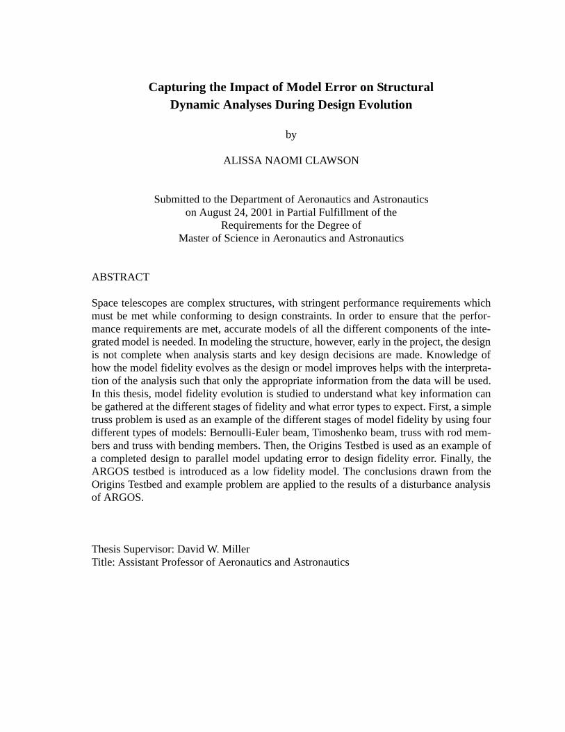
Mosier, 1998a, Robertson, 1997]. Figure 1.5 is an example of an integrated model
matic. The highlighted portion within the dotted lines is the integrated model. The inp
unit intensity white noise, d, and the outputs are the performances metrics, z. The
within the shaded region are the individual components of the integrated model. Th
lowing description of the integrated modeling is based on the work of Homero Gutier
The “Opto-Structural Plant” block in Figure 1.5 represents the structural model of
The model is built using finite element methods and represented in state-space form
structural model represents the dynamics of the system, and accepts forces, f, as in
outputs the states, x, of the system as shown in Figure 1.6.
Performance metrics are use to determine if the telescope meets the engineering
ments, thereby accomplishing its science objectives. Two examples of performanc
shown in Figure 1.5: OPD and pointing. The OPD metric is shown as the RMS of the
28 INTRODUCTION
Figure 1.5 Example Integrated Model: SIM
Figure 1.6 block diagram representation of precision controlled opto-structural integrated model
Process Noise
Opto-Structural PlantSIM V2.2 2184 states
W hite Noise Input
ACS
Perform ances (z)
Phasing (OPD)
Pointing (W FT)
σz,2 = RSS W FT
Appended LTI System Dynam icsAppended LTI System Dynam ics
(RW A broadband)
d
w
u y
z
Σ
Σ
Sensor Noise
σz,1=RMS OPD
#1#2
#3#4
#5#6
#7#8
Intr #1 Intr #2 Intr #3
Telescope #
OpticalControl
(RW A discrete)
(Star Tracker)
Inputs (W)1: RWAFx2: RWAFy3: RWAFz
4: RWATx5: RWATy6: RWATz
Outputs 1-18Star OPD #1-3Internal Metrology #1-3Star X/Y WF 1/2 Tilt #1-3
Outputs 19-30, 34Front End Cam X/Y WF 1/2 Tilt #1-3External Metrology Pathlength
z
Outputs (y) 31-33Attitude Angle X/Y/Z
y
Ad,Bd,C d,D d
d
Ap,Bp,C p,D p
F x C z zβw
wplant
controller
βuC y
yuAc,Bc,C c,D c

Integrated Modeling 29
lant
s, x, to
equires
lating
odels
e
uctural
in the
r. The
ure 1.6,
distur-
ilter or
atrices,
nces, a
input
con-
e. The
distur-
history. The pointing error, or wavefront tilt (WFT) is given by the root sum squared (rss)
of the radius of the time history. The pointing time history information is shown projected
on the plane of the telescope’s receiver.
The performance block, Cz, is not shown in Figure 1.5 because it is modeled in the p
model. The state-space matrix that is represents linearly combines the system state
produce the output metric(s), z. Calculating space telescopes performance metrics r
creating a sensitivity matrix from the plant states to the performance metrics. Calcu
these sensitivities require structural engineers and optical engineers to fuse their m
together.
In Figure 1.6, w is the disturbance force and the block, βw, represents the state-spac
matrix that maps the disturbances onto the appropriate degrees of freedom in the str
model. This block is also not shown in Figure 1.5, because it, too, is contained with
plant model.
The disturbances can be input into the structural model as a white noise shaping filte
disturbance filter has its own states and state-space representation as shown in Fig
where d is the white noise input and w is the shaped disturbances. Modeling the
bances involves either determining the time histories or creating the state-space f
both. The subscripts d and p denote the disturbance verses the plant state space m
respectively.
If the plant does not meet the performance requirements in the presence of disturba
controller may be used to improve the system performance. In Figure 1.6, output y is
to the controller and the controller output, u, drives the plant. All blocks except the
troller are part of the plant’s state space representation as indicated by the dotted lin
complete integrated model has the state-space formulation of the plant dynamics,
bance filter and the controller.

30 INTRODUCTION
end in
proto-
f inte-
eration
und.
the
redic-
starts
e low
1.3 Thesis Objective
1.3.1 Importance of Accurate Structural Models
Section 1.1.1 and Section 1.1.2 introduced the difficulty of designing space telescopes to
achieve the science goals of the Origins Program. The term nanodynamics appropriately
implies the degree of precision to which the structures must be controlled.
The fundamental reason why analytical models are used to predict the capabilities of the
design is because some structures can not be built for testing; also, the environment the
system is being designed for cannot be adequately reproduced [Moses, 1998]. At the con-
ceptual design stage, multiple architectures are compared to determine the direction for
future development. Once an architecture is chosen, a number of design iterations are per-
formed before the actual spacecraft is built and deployed. The performance must be able
to be predicted through structural analysis to assess the design without building the struc-
ture at each iteration. Analytical modeling provides major cost and time savings by doing
as much analysis on computers as possible instead of experimentally.
Besides time and cost savings, some telescopes are impractical to build for ground testing.
NGST’s sunshield, approximately the size of a tennis court, is an example of the tr
future designs towards increasingly larger spacecraft. Though individual subsystem
types are built for testing, the size of the complete spacecraft limits the practicality o
grating the entire structure on the ground. Space structures are also designed for op
in a zero-g environment, and may not be able to support their own weight on the gro
Without ground test verification, the analytical model must accurately capture
dynamic behavior of the structure in order to have confidence in the performance p
tions. Early in the project, however, the design is not fully complete when analysis
and key design decisions are made. It is important to know what information from th
fidelity models can be used to make these critical decisions.

Thesis Objective 31
itera-
final
en its
n the
s the
roves
it is
odel.
ncept
a flow
mined
must be
ure is
is cho-
s, more
are cho-
r in the
proper-
etween
exist-
1.3.2 Model Fidelity
The accuracy of a model can only be as good as the maturity of the design it is based upon.
The maturity of the design refers to how well the iteration represents the final version. If
the iteration is in the conceptual design stage, analysis will not accurately reflect the char-
acteristics of the finished product. If the iteration is near final, then its model will still not
reflect the actual behavior of the “true” system, but will have less error than the low
tion model and the dynamics will more closely resemble the actual behavior of the
system. If the iterations are complete and the structure is being built or is built, th
model will represent the behavior of the system only to the uncertainty that is withi
model itself and not due to uncertainties in the design [Berman, 1999]. Hence, a
design iterates and stabilizes towards the final solution, the fidelity of the model imp
and becomes more reliable for predicting performance. In studying model fidelity,
important to understand how the behavior of low fidelity models resemble the truth m
Low fidelity designs occur at the beginning of the design process, when a mission co
and architecture are chosen. The design requirements are determined based on
down from the science requirements. For example, a maximum OPD RMS deter
necessary for mission success is used to determine the extent that the structure
made rigid, isolated, or controlled. At this stage, only a basic overview of the struct
known with general dimensions in order to keep the optics it its nominal positions.
From the different possible architectures to satisfy the requirements, one approach
sen that satisfies the cost, requirements and constraints. As the design progresse
subsystem requirements are determined, dimensions of components and materials
sen, and a more detailed layout of the structure is created. Fidelity increases furthe
design process when the design becomes fixed and most dimensions and material
ties are known.
To understand the errors associated with model fidelity, an analogy can be made b
the model evolution of a design in progress and the model updating evolution of an

32 INTRODUCTION
r values
a sim-
pdated.
arame-
param-
and a
by
. As
h the
edomi-
ss) of a
ciated
impler
alled a
amics
g as
truss,
ainty in
ing structure. This analogy is helpful because model updating is a well-researched topic;
there is ample material on the errors associated with fidelity error of the model of a single
design iteration [Berman, 1999]. Joshi et al. discuss model fidelity in the sense of model
updating, where the increasing fidelity models are the increasingly accurate models of the
same built structure [Joshi, 1997].
The updating process begins with a model based on simplifying assumptions and nominal
material properties gathered from look-up tables. The model improves as the assumptions
are checked for accurate representation of the structure’s behavior and as paramete
are tested [Glease, 1994]. The model evolution of the design in progress undergoes
ilar process, assuming that the models compared at each iteration have been u
These models are based on a design that has simplifying assumptions and lack of p
ter value knowledge. As the design evolves, the assumptions are solidified and the
eter choices are made. Thus there is a local model evolution within model updating
global model fidelity evolution as a structure is being designed, as illustrated
Figure 1.7.
This analogy can help explain the types of errors involved in model fidelity evolution
the term “evolution” implies, there is a change in the type of errors associated wit
model at the different design stages. In the earlier stages, non-parametric errors pr
nate. These are errors that cannot be associated by a parameter (mass or stiffne
model element, but are akin to a “lack” of a parameter. Early design errors are asso
with errors in design assumptions.
In early design stages and for initial models, large structures can be modeled by a s
element, such as representing a truss by a beam element. This simplified model, c
stick model, saves computational time when conducting analysis. The beam’s dyn
will resemble the global, fundamental characteristics of the truss while not requirin
many elements. The beam will not adequately resemble all the characteristics of the
but because the parameters, configuration and dimensions are not fixed, the uncert

Thesis Objective 33
the design is on the same order of magnitude or larger than that associated with the inaccu-
racies of the stick model.
Figure 1.7 Model Fidelity Evolution
Figure 1.8 Uncertainty [Gutierrez, 1999]
Design Evolution
Model U
pdating
2nd1st
Iteration3rd ...
Structural Design Accuracy
Analytical M
odel Accuracy
Flight
M odel Fidelity Evolution
Decoupled M odel Progression
Actual Progression of M odel
Initial M odel
Final Updated M odel
D esign Iteration
Performance
21 3 4
R equirem ent
E rror B ounds
N om inal S olution

34 INTRODUCTION
Figure 1.8 illustrates the performance prediction and error bounds for four design itera-
tions of an imaginary system. The vertical scale in Figure 1.7 can be paralleled with the
error bounds of Figure 1.8, where as the error bounds decrease, the analytical model accu-
racy increases. For Design 1, the performance prediction does not meet the requirement.
For Design 2, the design is improved until the nominal solution meets the requirements,
but the addition of the error bars shows that the design may or may not meet the require-
ment. Designs 3 and 4 are two different approaches from Design 2. Design 3 improves the
design so that with the uncertainty, the design will meet the requirements. Design 4 does
not change the design, but reduces the uncertainty.
Thus there are two ways that the error bars can be defined. The first is with accurate mod-
eling but a low iteration design and the second is with a finalized design but a poor analyt-
ical model. Both of these types of error sources can contribute to poor model fidelity. The
objective of this thesis is to look at model fidelity evolution compared to model updating
to understand how the behavior of low fidelity models resembles the truth model.
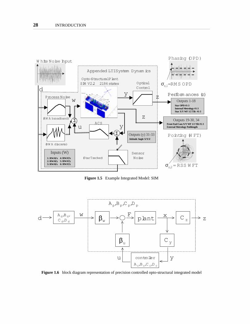
1.4 Dynamics Optics Controls Structures (DOCS)
The Space Systems Laboratory at MIT has developed a set of software modules and a
design and analysis methodology for precision space telescopes called DOCS. DOCS
stands for Dynamics Optics Controls Structures and a flowchart for the methodology is
shown in Figure 1.9.
The first step in DOCS is modeling all the components of the integrated model. Starting
with the design of a telescope, the structure and optics models are created and the distur-
bance sources are determined and modeled. Since reaction wheels are the primary distur-
bance source for space telescopes, a lot of work has been done to model their disturbances.
Work on reaction wheel modeling has been done by Rebecca Masterson
[Masterson, 1999] and Laila Elias [Elias, 2001].
Dynamics Optics Controls Structures (DOCS) 35
e met-
f mag-
grees
oller.
le, and
condi-
l anal-
meet
The individual models are then assembled in the next stage of DOCS. Before being ana-
lyzed, however, the model must be updated, conditioned and reduced. The necessity of
conditioning is a by-product of using computers to analyze structures. Poor numerical
conditioning can cause problems in the analysis not related to the inherent design. For
example, if the units of the structure’s dimensions are in meters and the performanc
rics are in nanometers, the model will be handling two sets of numbers nine orders o
nitude apart. Additionally, the final model can have an extremely large number of de
of freedom with the addition of the dof’s of the disturbance model and the contr
When converted to modal coordinates, not all modes are observable or controllab
are unnecessary additional information adding to computational expense. Work on
tioning and model reduction has been done by Scott Uebelheart [Uebelhart, 2001].
After preparing the model, it then moves to the next stage, analysis. The fundamenta
ysis that is done is the disturbance analysis, which will determine if the model will
Figure 1.9 DOCS Flowchart
Design Structural ModelStructural Model
DisturbanceSources
DisturbanceSources
Measurem ent ModelMeasurem ent Model
UncertaintyDatabase
UncertaintyDatabase
Baseline Control
Baseline Control
Model Reduction &Conditioning
Model Reduction &Conditioning
ModelAssem bly
ModelAssem bly
ModelUpdating
ModelUpdating
DisturbanceAnalysis
DisturbanceAnalysis
Sensor &ActuatorTopologies
Sensor &ActuatorTopologies
ControlForgeControlForge
Data
SystemControlStrategy
M odeling Model Prep Analysis Design
ControlTuning
ControlTuning
Optical ModelOptical Model
Isoperform anceIsoperform ance
SubsystemRequirem ents
ErrorBudgets
Optim izationOptim ization
SensitivitySensitivity
Σ Margins
System Requirem ents
Inputs Software Modules Outputs
UncertaintyAnalysis
UncertaintyAnalysis

36 INTRODUCTION
d is
lt. The
dating
the performance. The disturbance analysis methods used in the Space Systems Lab and in
this thesis were developed by Homero Gutierrez [Gutierrez, 1999]. Disturbance analysis
can be done open or closed loop. If the model does not satisfy the performance require-
ments open loop, then a controller is added to the system. Greg Mallory did work on con-
troller tuning for space telescopes based on measurement models [Mallory, 2000a].
Mathematical models of real systems inherently have errors associated with them because
the models contain assumptions and simplifications in order to be made. While the distur-
bance analysis may predict that the model meets the performance requirements, the uncer-
tainty analysis determines the error bounds about this prediction [Bourgault, 2000].
After completing the analysis, the results are studied in the design stage. If the model does
not meet the performance requirements, then a change in the controller and/or a change in
the telescope design must be made. Sensitivity analysis determines how the changes in
parameters affect the performance of the system. If the model does meet the performance
requirements, design of the system is not necessarily over. An isoperformance analysis
finds multiple sets of design parameters that result in the same performance. This analysis
can be important during manufacturing considerations; as some subsystems, like reaction
wheels or optical sensors, do not have a continuous array of sizes or quality to choose
from parameters traded. Also, improving the performance of one subsystem may be less
expensive than improving the performance of another. Work on isoperformance is being
done by Olivier de Weck [DeWeck, 1999].
1.5 Thesis Overview
Figure 1.10 illustrates how the organization of the chapters in this thesis fits in with the
model fidelity evolution diagram of Figure 1.7. First, in Chapter 2 a two-dimensional truss
structure is used as an example problem that demonstrates the evolution of a low fidelity
“stick” model to a high fidelity “truth” model. Then, in Chapter 3, the Origins Testbe
given as an example of a high fidelity design - a structure that has already been bui
analytical model updating of the testbed is used as a demonstration of the model up

Thesis Overview 37
error analogy to design evolution. In Chapter 4, the ARGOS testbed is described as an
example of a low fidelity model. A disturbance analysis is done on ARGOS and conclu-
sions on the analysis are drawn based upon knowledge of ARGOS’ model fidelity.
Figure 1.10 Thesis Roadmap
Low FidelityDisturbance AnalysisARG O S Testbed
Chapter 4
High FidelityM odel UpdatingO rigins Testbed
Chapter 3
M odel Fidelity EvolutionSam ple Problem
Chapter 2
FlightConceptDesign

38 INTRODUCTION
Chapter 2
SAMPLE PROBLEM
modal
eate the
rmonic
ystem.
pring
e force
In this chapter, a truss sample problem is presented to describe the different stages of
model fidelity. The design maturity is simulated by different finite element types: (listed in
order of increasing fidelity) a Bernoulli-Euler beam, a Timoshenko beam, a truss with rod
elements and a truss with bending beam elements. Model updating is simulated by mesh-
ing the finite elements at different degrees of refinement. The models are compared to a
“truth” model, which is the highly refined truss with bending elements.
2.1 State Space Representation
In this section the state space representation of equations of motion in structural
form is derived. Then the disturbance states are appended to the plant states to cr
integrated model. State space representation is first introduced using a simple ha
oscillator as an example, and is then applied to a discrete multi-degree of freedom s
The 1-dof harmonic oscillator is shown in Figure 2.1, where m is the mass, k is the s
constant, c is the damping coefficient, x is the displacement of the mass and F is th
applied to the mass.
The equation of motion for the mass is given by:
(2.1)
Then solving for the acceleration of the mass gives:
mx·· cx· kx+ + F=
39

40 SAMPLE PROBLEM
(2.2)
Two new variables x1 and x2 are defined such that:
(2.3)
Written in matrix form, the equation for the time derivatives of the new variables, x1 and
x2, using equations (2.2) and (2.3) are:
(2.4)
The vector, [x1, x2]T, contains the states of the system. Equation (2.4) is helpful for visual-
izing the state space representation since it still retains the physical characteristics of the
system. The derivation of the structural modal form for the multi-degree of freedom sys-
tems is based on the physics of the structure, but the resulting equations are in modal coor-
dinates, which are less physically intuitive. Notice from equation (2.4) that the number of
Figure 2.1 Simple system
m
k
c
x
F
x··cm----–
x·km----–
xFm----+ +=
x1 x≡
x2 x·≡
t
x1
x2
0 1
km----–
cm----–
x1
x2
0
Fm----
+=

State Space Representation 41
states is twice the number of degrees of freedom of the system. This fact always holds
when converting to a physically-based state-space representation.
For discrete systems with more than one degree of freedom, the mass and stiffness terms
are matrices instead of scalars. The equations of motion of a conservative (undamped),
linear, time invariant (LTI) system can be written as:
(2.5)
where M and K are the ( ) mass and stiffness matrices, respectively, x is a vector of
the n degrees of freedom (DOF) in the physical coordinate system, and F is a vector of
external forces acting on the system.
Assuming that the homogenous solution of equation (2.5) is of the form:
(2.6)
and substituting this solution into equation (2.5) while setting F = 0, we obtain:
(2.7)
Then, by substituting and rearranging, we obtain the generalized eigenvalue prob-
lem:
(2.8)
where λi is the ith eigenvalue and φi is the corresponding eigenvector. The index, i, ranges
from i = 1...m, where m is the number of modes of the system, ( ). In general, the
total number of modes is equal to the number of DOF, but it is not always necessary to
include all modes in the model. For instance, when using finite element methods, the
higher modes are often neglected. They inherently have high error due to the linearization
of finite elements and they add to the computational expense for large models. Addition-
ally, if the analytical model is compared to data, the higher modes may exceed the fre-
quency of the data and are then unnecessary information.
Mx·· Kx+ F=
n n×
x φejωt=
ω2Mφ– Kφ+ 0=
ω2 λ≡
K λiM–( )φi 0=
m n≤

42 SAMPLE PROBLEM
Due to the orthogonality of the eigenvectors, the following relationships hold:
(2.9)
where Φ is the ( ) eigenvector matrix. The superscript, 0, indicates that is mass
normalized. The columns of are the eigenvectors φ1, φ2, φ3,..., φm, I is the identity
matrix, and Ω2 is a diagonal matrix whose elements are the eigenvalues λ1 = ω12, λ2 =
ω22, λ3 = ω3
2, ... , λm = ωm2.
Using equation (2.9), equation (2.5) can be decoupled through a coordinate transformation
from physical to modal coordinates. Substituting:
(2.10)
into the equation of motion we obtain:
(2.11)
where ξ is the vector of modal coordinates.
Pre-multiplying equation (2.11) by gives:
(2.12)
Then using equations (2.9) and (2.11), we rewrite equation (2.12) as:
(2.13)
At this stage we add damping back to the system by assuming that the damping is propor-
tional to the modes. This assumption is valid for lightly damped systems:
(2.14)
Φ0 TM Φ0
I=
Φ0 TK Φ0
\
ωi2
\
Ω2= =
n m× Φ0
Φ0
x Φ0 ξ=
M Φ0 ξ·· K Φ0 ξ+ F=
Φ0 T
Φ0 TM Φ0 ξ·· Φ0 T
K Φ0 ξ+ Φ0 TF=
ξ·· Ω2ξ+ Q=
ξ·· 2ZΩξ· Ω2ξ+ + Q=

State Space Representation 43
where Z is the diagonal matrix of damping coefficients.
The forcing term is partitioned into two components: forces from disturbances, Fw, and
forces from control actuators, Fu:
(2.15)
where the ( ) matrix, βu, and ( ) matrix, βw, map the actuator forces and dis-
turbances, respectively, onto the correct degrees of freedom, nu are the number of actuator
inputs and nw are the number of disturbance inputs. The matrix completes the coordi-
nate transformation so that the actuator forces and disturbances act on the correct modal
coordinates. Substituting into equation (2.14) and rearranging we have:
(2.16)
Equation (2.16) is the equation of motion in the modal coordinate system. It is rearranged
as a system of equations and written in matrix form by defining a new state variable:
(2.17)
Then the equations of motion in state-space form are:
(2.18)
where A is the plant dynamics matrix, m is the number of modes retained Bu is the plant
actuation input matrix, nu is the number of controller inputs, Bw is the plant disturbance
input matrix, nw is the number of disturbance inputs.
Equation (2.18) is written in the structural-modal form. This form is most useful when the
mass and stiffness matrices are unknown, but the eigenvalues and eigenvectors are known.
Q Φ0 TF Φ0 TFu Φ0 TFw+ Φ0 Tβuu Φ0 Tβww+= = =
n nu× n nw×
Φ0 T
ξ·· 2ZΩξ·– Ω2ξ– Φ0 Tβuu Φ0 Tβww+ +=
qpξ
ξ·≡
p p 0 T 0 T2u w
(2m×2m) (2m×n ) (2m×n )u u w w
0 00
- -2
= + + Φ β Φ βΩ Ω
Iq q u w
Z
A B B
&1442443 14243 14243

44 SAMPLE PROBLEM
To complete the state space representation, the output is written as a combination of the
state variables:
(2.19)
where C maps the correct degrees of freedom to the output. To transform to modal coordi-
nates, is substituted in equation (2.19). To rewrite equation (2.19) in matrix
form, ξ and are factored out and replaced by qp to obtain:
(2.20)
where Cy is the plant output matrix and ny is the number of outputs. The matrices Dyu and
Dyw are the feedthrough matrices from the control forces and disturbances, respectively, to
the output and are usually zero.
Similarly, the performance can be written:
(2.21)
where Cz is the performance matrix, and nz is the number of performances. The matrices
Dzu and Dzw are the feedthrough matrices from the control forces and disturbances,
respectively, to the performance and are usually zero. The difference between y and z is
that the outputs, y, are the sensor measurements used by controllers for calculating actua-
tor control signals and the performances, z, are the metrics used to determine if the plant is
meeting requirements.
The complete state space system for the plant is thus written:
y Cx Dyuu Dyww+ +=
x Φ0 ξ=
ξ·
0 0
yx yx p yu yw
(n ×n ) (n ×n )(n ×2m) yu y u yw y wy y
= Φ Φ + + y C C q D u D w
D DC
& 123144424443
[ ] [ ]0 0
zx zx p zu zw
(n ×n ) (n ×n )(n ×2m) zu z u zw z uz z
= Φ Φ + + z C C q D u D w
D DC
&144424443
State Space Representation 45
(2.22)
A state-space model can be derived through an analytical model of the M and K matrices.
If the structure being modeled has already been built, then the analytical model can be
compared to the experimental data. Noise is input at the correct location and data are taken
from sensors at the output nodes. A set of A,B,C,D matrices is then found that best fits the
system ID transfer function. This model is called the measurement model and is assumed
to be a more accurate representation of the plant dynamics than the analytical model
[Marco-Gomez,1999]. Unfortunately, the measurement model is not created based on
relationships among physical parameters and, therefore, must be recalculated anytime the
structure or environmental conditions change.
Disturbance states:
As described in Section 1.2, disturbance can be modeled as a state space filter through
which unit intensity white noise is shaped to produce a Power Spectral Density (PSD)
with the equivalent energy and frequency content as the actual PSD of the disturbance.
The disturbance represented in state space form is denoted by a subscript d:
(2.23)
where qd are the disturbance states, d is the white noise input, and w is the shaped distur-
bance output.
A new state vector is created by appending the disturbance states to the plant states:
(2.24)
qp· Apqp Buu Bww+ +=
y Cyqp Dyuu Dyww+ +=
z Czqp Dzuu Dzww+ +=
qd· Adqd Bdd+=
w Cdqd=
qqd
qp
=

46 SAMPLE PROBLEM
bend-
d the
ls only
idual
shenko
an the
and the system equations are:
(2.25)
where d is the white noise input and z is the performance output.
2.2 Problem Formulation
A simple truss is used as a sample problem to illustrate the evolution of model fidelity,
which is the increase in the accuracy of the model as the design iterates to the true system.
The initial design is a simple beam and the final design is a beam-like truss. To adequately
compare the low fidelity beam-type model with the high fidelity truss model, the beam is
forced to have properties equivalent to the final truss design. In an actual design scenario,
where the final design is not known a priori, the initial design will include parametric
errors in addition to the non-parametric errors discussed in this section.
In this example, model fidelity evolution is demonstrated through the use of different
finite elements and by refinement of the finite element mesh. The truss is first represented
as a stick model with Bernoulli-Euler beam elements and then with Timoshenko beam ele-
ments. The next step in the model evolution is to accurately model the truss geometry.
However, the truss is first modeled using rod members which only have forces and dis-
placements in each member’s axial direction. Finally, the members are modeled as
ing members. A highly refined model of the truss with bending members is considere
“truth” model against which to compare the others.
The type of finite element determines the modes that are modeled. The stick mode
capture the global modes of the truss and not the effects of the flexibility of the indiv
truss members. Because the truss has a low aspect ratio (length/depth) the Timo
beam captures the truss’ global bending modes at a significantly higher accuracy th
q·Ad 0
BwCd Ap
qBd
0d+=
z 0 Czq 0 d+=

Problem Formulation 47
Bernoulli-Euler beam. A truss modeled with rods does not capture the local bending
modes of the members, but captures the stiffness characteristics of the truss more accu-
rately than the beam elements. Finite element mesh refinement increases the number of
modes calculated and allows the lower-frequency modes to converge to the continuous
solution.
The truss consists of eight square bays with alternating diagonals across each face. It is
fixed at one end, x = 0, and free at the other, x = L. The members of the truss are circular
beams of radius r. The horizontal and vertical members have length (Lm = L/8) and the
diagonal members have length Lm. The nodes are labeled across the top from left to
right then across the bottom from left to right. A downward force is applied to the top of
the truss at node 6, and the performance is the truss tip displacement as shown in
Figure 2.2. The truss configuration and property values resemble one face of the three
dimensional truss tower of the Origins Testbed. However the total length was fixed to 1m
for numerical simplicity. The property values are listed in Table 2.1.
2.2.1 Equivalent Inertia
An advantage of modeling a truss with a stick model is the reduction of the number of
degrees of freedom and thus the reduction of the size of the model and computational
time. However, to accurately represent the truss as a beam, the stick model must have sim-
ilar fundamental characteristics, such as static deflection (static similarity) and/or funda-
Figure 2.2 Example problem truss schematic
2
Force Displacem ent
L
LM
48 SAMPLE PROBLEM
mental mode(s) (dynamic similarity). A simple analysis of the truss is deformed to
determine the equivalent beam properties. Then the beam is used for analysis of the larger
system.
Sun et al. present a method to find the equivalent properties for a truss [Sun, 1981]. The
authors solve for the three equivalent beam stiffnesses: e.g. axial stiffness (EA), bending
stiffness (EI), and shear stiffness (GA) assuming that these properties are decoupled.
Necib et al. discusses how to calculate the entire matrix of coupled stiffnesses as well,
which is important for asymmetrical structures [Necib, 1989]. The decoupled stiffnesses
will be used for the sample problem. The equivalent inertia properties of the truss are the
mass per unit length (ρA) and the rotary inertia per unit length (ρI) and their calculations
are also presented by Sun et al.
Because equivalent beam properties are calculated via static deflections of the truss, the
following derivation is for a simple, static truss using ideal truss assumptions: members
experience only compression and tension [Strang, 1986]. Each node has two degrees of
freedom as shown in Figure 2.3. There are eighteen nodes and 33 members.
The vector, x, is a vector of unknown displacements at each node, where superscripts H
and V specify horizontal and vertical displacement, respectively:
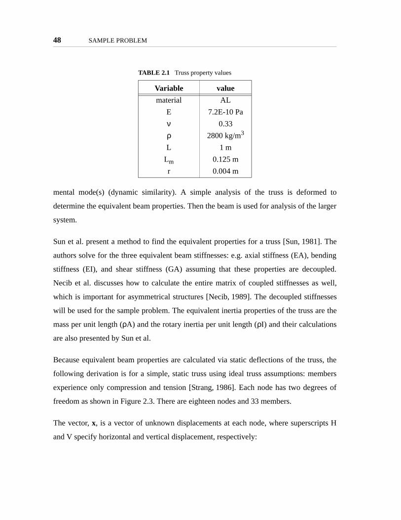
TABLE 2.1 Truss property values
Variable value
material AL
E 7.2E-10 Pa
ν 0.33
ρ 2800 kg/m3
L 1 m
Lm 0.125 m
r 0.004 m

Problem Formulation 49
(2.26)
The vector, e, is a vector of elongations, where ei is the elongation of the ith member:
(2.27)
The elongations are calculated via the geometry of the truss. The following is an example
of the equation for the elongations of members 2 and 14:
(2.28)
The set of equations for e is written in matrix form such that:
(2.29)
where A is the ( ) incidence matrix, m is the number of members and n is the number
of nodes. The internal force in member i, yi, is determined via the beam constitutive equa-
tion:
Figure 2.3 Labeling of the truss (left four bays shown)
1 2 3 4 5...
29
1 2 3 4
9 10 11 12
26 27 28
x1
x1
x2
x2
V
H H
V
10
13 14 15 16 17...
11 12 13 14...
x x1H
x1V
x2H
x2V … x18
VT
=
e e1 e2 e3 … ei … e33=
e2 x3H
x2H
–=
e141
2-------x4
H 1
2-------x12
H–
1
2-------x4
V 1
2-------x12
V–+=
e Ax=
m n×

50 SAMPLE PROBLEM
(2.30)
where Ei is the modulus of elasticity of the ith member, Ai is the cross-sectional area and
Li is the length of the member. The product, EiAi, is the axial stiffness and is the same for
all members. Only Li is different and is 0.125m for the horizontal and vertical members
and *0.125 for the diagonal members.
Equation (2.30) can be written in matrix form
(2.31)
where the diagonal matrix, C, is formed with the elements, ci, along the diagonal.
Finally, the nodal force, f, is the sum of the internal forces from each member connected to
the node. The equilibrium equation is written:
(2.32)
Combining equations (2.29), (2.30), and (2.32), produces a relationship between the nodal
forces, f, to the displacements, x:
(2.33)
Axial Stiffness
To calculate the equivalent axial stiffness, EA, for the truss, constrain the truss such that
node 10 is pinned and node 1 is free to move vertically (Figure 2.4). A force of -1N is
applied at the right end of the truss by applying 0.5 N at nodes 9 and 18 in the negative xH
direction.
The deflection of the tip nodes as a result of the compressive force is related to the axial
stiffness by:
yi ciei=
ci
EiAi
Li-----------=
2
y Ce=
ATy f=
x ATCA( ) 1– f=

Problem Formulation 51
(2.34)
where F is the applied force, L is the total length, ∆x is the change in length of the truss, E
is the modulus of elasticity and A is the cross-sectional area. The displacement of nodes 9
and 18 are both calculated to be from Equation (2.32) -1.382x10⁻⁷m, and then Equation
(2.34) gives EA = 7.238x10⁶N.
Bending Stiffness
The bending stiffness, EI, is calculated by decoupling the bending and shear deflections. A
moment is applied at the end of the truss and the truss is constrained the same as for the
compression test. A force of 1N is applied at node 9 in the positive horizontal direction
and a force of 1N is applied to node 18 in the negative horizontal direction to create a
bending moment of 0.125Nm (Figure 2.5).
The resulting angular deflection, φ, of the end member is related to the bending moment
by:
(2.35)
Figure 2.4 Axial Compression
0.5N
0.5N
∆x
xH
xV1
10
9
18
L
∆xFLEA--------=
M F Lm× EIφ
Lm-------= =

52 SAMPLE PROBLEM
where M is the moment acting on the beam, Lm is the moment arm, E is the modulus of
elasticity, I is the inertia and φ is the tip angular displacement due to bending. The angle,
φ, is assumed to be small. The resulting displacement of node 9 is xH = 2.762e-7,
xV = 1.105e-6 and node 18 is xH = -2.762e-7, xV = -1.105e-6 from Equation (2.33). The
resulting bending stiffness calculated from equation (2.35) is EI = 2.2619x10⁵Nm2.
Shear Stiffness
The shear stiffness, GA, is calculated by applying a shear force of 1N at the end of the
truss and constraining nodes 1, 9, 10, and 18 such that the truss cannot bend, but can only
deflect due to shear deformation. Node 10 is pinned and nodes 1, 9 and 18 are only free to
move vertically (Figure 2.6).
The resulting angular deflection, θ, is related to the shear force by:
(2.36)
where Q is the shear force, G is the shear modulus of elasticity, A is the cross-sectional
area, and θ is the total angular deflection due to the applied force. From Equation (2.33),
the vertical displacement of node 9 is calculated to be 1.645x10⁻⁶m, and node 18 is calcu-
lated to be 1.610x10⁻⁶m. These two results are averaged to obtain an average displacement
and then the equivalent shear stiffness, GA = 2.6113x10⁵N, from Equation (2.36).
Figure 2.5 Bending Moment
1N
1N
φxH
xV
1
10 18
9
Lm
Q GAθ=

Problem Formulation 53
Mass Per Unit Length
The the mass per unit length for the equivalent beam is given by m = ρA. This term is cal-
culated by dividing the mass of the truss by its total length. The mass of the truss is calcu-
lated from the volume of each member (VVH = πr2Lm or πr2 Lm), the density of
aluminum (2800 kg/m3) and the number of members.
(2.37)
where nHV is the number of horizontal and vertical members, ndiag is the number of diago-
nal members, LHV = Lm, and Ldiag = Lm. The mass per unit length, ρA, for the sample
truss is 0.6389 kg/m.
Rotary Inertia Per Unit Length
Timoshenko beams account for the rotary inertial effects of the beam. The rotary inertia
appears in the equations of motion as the product, ρI, which is the inertia per unit length
about an axis perpendicular to the plane of the truss through the centerline. The rotary
inertia per unit length is equivalent to the rotary inertia about the centerline divided by the
total length.
Figure 2.6 Shear Force
0.5N
0.5N
θ
2
ρAnHV π r2 LHVρ ndiag π r2 Ldiagρ+
L--------------------------------------------------------------------------------=
2

54 SAMPLE PROBLEM
(2.38)
where nH is the number of horizontal members, nV is the number of vertical members,
ndiag is the number of diagonal members, LHV = Lm, and Ldiag = Lm.
Calculating the inertia about the centerline gives the rotary inertia per unit length because
an infinitesimal cross section of the truss (perpendicular to the centerline) has the same
inertia when rotated about the point of intersection with the centerline in any direction
(Figure 2.7).
The rotary inertia, ρI, calculated for the truss is 0.0016 kg.m.
Equivalent Material and Beam Properties
In order to implement the beam model in MSC/NASTRAN, the material properties (E, G
and ρ) and the beam properties (A,I) are required individually, not as products (EA, EI,
GA, ρA, and ρI). Unfortunately, the five products cannot be used to produce five unique
quantities, E, G, ρ, A, and I. If the product EA is dividing by EI to obtain the ratio,
Figure 2.7 Rotary inertia per unit length is equivalent to the inertia of the truss calculated about the cen-terline, rotating in and out of the plane divided by the total length
ρI
nHρALHV
2----------
2
nVρALHV
3( )12
--------------- ndiagρALdiag
3
12------------
LHV
Ldiag------------
2+ +
L------------------------------------------------------------------------------------------------------------------------------------------=
2
centerline
LHV2
LdiagLHV
infinitesim alcross section
rotary inertia direction

Problem Formulation 55
n
r and
utions
te ele-
ation
2.8,
s the
e con-
, and the same is done for the products ρA and ρI to get another value for
the ratio, , then these two ratios are equal when calculated for real beams
and materials. However, these products were determined by finding equivalent beam
properties and they do not equal each other in this example. Because rotary inertia terms
are small, the errors from removing the ρI term should be small [Sun, 1981] and then the
rest of the products can be used to find the equivalent material and beam properties. By
setting E to be Young’s modulus for aluminum (7.2x10¹⁰Pa), the other four quantities ca
be solved.
2.2.2 Continuous Beam Solutions
In this section, the natural frequencies and mode shapes for the Bernoulli-Eule
Timoshenko beams are derived from continuous formulations. These analytical sol
serve as a benchmark against which to compare the effect of refinement of the fini
ment models on the accuracy of the dynamic predictions.
Bernoulli-Euler Beam
The Bernoulli-Euler (BE) beam model assumes that rotary inertia and shear deform
are negligible. The continuous model of the Bernoulli-Euler beam is shown in Figure
where m(x) is the mass per unit length, E(x) is the modulus of elasticity, and I(x) i
inertia of the cross-sectional area, A(x) is the cross-sectional area. All properties ar
stant with respect to x in this example.
The partial differential equation (PDE) of a Bernoulli-Euler beam is:
TABLE 2.2 Equivalent beam properties
E 7.200 e10 Pa
G 2.598 e9 Pa
ρ 6345 kg/m3
A 1.005 e-4 m2
I 3.142 e-6 m4
A/I EA/EI=
A/I ρA/ρI=

56 SAMPLE PROBLEM
(2.39)
where indicates the fourth derivative with respect to x and indicates the deriva-
tive with respect to time. The beam is fixed at x = 0 and free at x = L. The corresponding
boundary conditions for this configuration are:
(2.40)
The initial conditions w(x,0) and (x,0) are given. For modal analysis, however, the ini-
tial conditions are not necessary.
The homogenous solution for the PDE is assumed to be a product of independent temporal
and spatial functions:
(2.41)
Substituting the solution into the PDE, we obtain:
(2.42)
Separating the functions of time, t, and space, x:
Figure 2.8 Truss modeled as beam
w (x,t)
L
m (x), E I(x), A (x)
x
EI wiv x t,( ) mw··+ f x t,( )=
( )iv ( )··
at x 0= w 0 t,( ) 0= wi
0 t,( ) 0=
at x L= EI wii
L t,( ) 0= EI wiii
L t,( ) 0=
w·
w x t,( ) W x( )F t( )=
EI Wiv x( )F t( ) mW x( )F··
t( )+ 0=

Problem Formulation 57
(2.43)
The temporal solution gives the relationship between the natural frequencies, ω, and the
eigenvalues, λ. The differential equation for the temporal solution is:
(2.44)
The general solution is assumed to be in the following forms:
(2.45)
where
(2.46)
The constants A and its complex conjugate,A, (or C and the phase, φ) are determined
from the initial conditions. The natural frequency, ω, is determined by solving the spatial
problem given by:
(2.47)
where
(2.48)
The solution of equation (2.47) is of the form:
(2.49)
The constants are determined through the boundary conditions:
F··
t( )F t( )---------- EI
m------ W
ivx( )
W x( )-----------------– cons ttan λ–= = =
F··
t( ) λF t( )+ 0=
F t( ) Aeiωt Ae iωt–+=
C ωt φ+( )cos=
λ ω2=
Wiv x( ) β 4W x( )– 0=
β mλEI--------4=
W x( ) Aeβx Be βx– Ciβx D iβx–+ + +=
C1 βxsinh C2 βxcosh C3 βxsin C4 βxcos+ + +=

58 SAMPLE PROBLEM
(2.50)
Non-trivial solutions are obtained by setting the determinant of the matrix equal to zero.
The resulting equation is:
(2.51)
Since the model is a continuous beam, there are an infinite number of solutions and thus
an infinite number of modes. The first eight solutions of equation (2.51) are: βL = 1.8750,
4.6940, 7.8550, 10.9960, 14.1370, 17.2790, 20.4200, 23.5620. These values of βL hold
true for all BE beams that have clamped-free boundary conditions.
The natural frequencies are calculated from βL by equations (2.46) and (2.48):
(2.52)
The natural frequencies are dependent upon the material and beam properties. Stiffer
beams (large EI) have higher natural frequencies and heavier beams (large mL) have
lower natural frequencies. Since there were originally five unknowns (C1-4 and β), and
four equations the system is under determined. However, if we set the value for one con-
stant, we can solve for the other three.
If C4 = -1, then:
(2.53)
W 0( ) 0= ⇒
Wi
0( ) 0= ⇒
Wii
L( ) 0= ⇒
Wiii
L( ) 0= ⇒
0 1 0 1
1 0 1 0
βLsinh βLcosh βLsin– βLcos–
βLcosh βLsinh βLcos– βLsin
C1
C2
C3
C4 0
0
0
0
=
βLcosh βLcos⋅ 1+ 0=
ωr λr βr L( )2 EImL4-----------= =
C1βLcosh βLcos+βLsinh βLsin+
-----------------------------------------–=
C2 1=
C3βLcosh βLcos+βLsinh βLsin+
-----------------------------------------=
C4 1–=

Problem Formulation 59
and the complete solution for W(x) is:
(2.54)
The mode shapes of the beam are obtained by substituting in the values of β and βL into
Equation (2.54). Note that the mode shapes are only dependent upon the boundary condi-
tions and the length of the beam. However, the length of the beam can be removed from
the mode shape expression through a non-dimensional variable ξ = x/L. Using the equiva-
lent beam parameters in Table 2.2, natural frequencies of the first eight modes are listed in
Table 2.3 and Figure 2.9 shows the first three mode shapes.
2.2.3 Timoshenko Beam
In the Bernoulli-Euler beam formulation rotary inertia and shear deformation are
neglected. This simplification is valid for slender beams at lower frequencies, but
degrades higher mode predictions. The effects become significant for thick beams and
slender beams at higher frequencies.
Shear effects are accounted for in the Timoshenko beam model by redefining the deflec-
tion angle as follows:
TABLE 2.3 Continuous Bernoulli-Euler Beam
Natural Frequencies
Mode # ωr [rad/s] fr [Hz]
1 2094 333.3
2 1.312e4 2089
3 3.675e4 5849
4 7.202e4 1.146e4
5 1.190e5 1.895e4
6 1.778e5 2.830e4
7 2.484e5 3.953e4
8 3.307e5 5.263e4
W x( ) βxcosh βxcos–( ) βxsinh βxsin–( )–βLcosh βLcos+βLsinh βLsin+
----------------------------------------- ⋅=

60 SAMPLE PROBLEM
elastic-
(2.55)
where w(x,t) is the translational displacement of the beam, ψ(x,t) is the angle of deflection
without shear effects (only due to the translational displacement) and β(x,t) is the angle of
deflection due to shear as shown in Figure 2.10.
Equation (2.55) includes two dependent variables, ψ and β. Substituting (2.55) into the
Timoshenko beam equations of motion results in a set of two dependent PDE’s:
(2.56)
where is the shear area factor, A is the cross-sectional area, G is the modulus of
ity in shear and J is the rotary inertia per unit length defined by the product, ρI.
Figure 2.9(a)Mode #1333.3 Hz
Figure 2.9(b)Mode #22089 Hz
Figure 2.9(c)Mode #35849 Hz
Figure 2.9 First three mode shapes for continuous Bernoulli-Euler beam
0 0.1 0.2 0.3 0.4 0.5 0.6 0.7 0.8 0.9 1 x
W (x)
0 0.1 0.2 0.3 0.4 0.5 0.6 0.7 0.8 0.9 1 x
W (x)
0 0.1 0.2 0.3 0.4 0.5 0.6 0.7 0.8 0.9 1 x
W (x)
x∂∂ w x t,( ) ψ x t,( ) β x t,( )+=
mw·· k'AG wii ψi
–( )– 0=
EIψiik’AG w
i ψ–( ) Jψ··–+ 0=
k'

Problem Formulation 61
)) is
le,
Decoupling equations (2.56) and writing two PDE’s in terms of ψ and w gives:
(2.57)
The following derivation of the solutions to the Timoshenko PDE (Equation (2.57
taken from Huang [Huang, 1961]. With the introduction of a non-dimensional variabξ,
the solutions for w(x,t) and ψ(x,t) are assumed to be in the following form:
(2.58)
Substituting Equations (2.58) into Equation (2.57) we obtain:
(2.59)
Figure 2.10 Deflection for Timoshenko beam [Meirovich, 1997] In a Bernoulli-Euler beam, β = 0.
Ψ(x,t)
Ψ(x,t)β(x,t)
dx
EIwiv
mw·· JEImk'AG-------------+
x2 t2∂
4
∂∂ w
–Jm
k’AG-------------
t4
4
∂∂ w
+ + 0=
EIψivmψ·· J
EImk'AG-------------+
x2 t2∂
4
∂∂ ψ
–Jm
k’AG-------------
t4
4
∂∂ ψ
+ + 0=
w ξ( ) Weiωt=
ψ ξ( ) Ψeiωt=
ξ xL---=
Wiv b2 r2 s2+( )W'' b2 1 b2r2s2–( )W–+ 0=
Ψiv b2 r2 s2+( )Ψ’’ b2 1 b2r2s2–( )Ψ–+ 0=

62 SAMPLE PROBLEM
where:
(2.60)
The boundary conditions for the cantilever beam are:
(2.61)
The solutions of equation (2.59) can be written as:
(2.62)
where
(2.63)
when the following condition holds
(2.64)
When the condition in Equation (2.64) is not met, as is the case for the sample problem,
substitute the solutions for W and Ψ are written as:
(2.65)
where is given by:
b2 mL4ω2
EI------------------=
r2 IAL2----------=
s2 EIk’AG-------------=
at ξ 0=
at ξ 1=
W 0( ) 0=
1L---W
i1( ) Ψ 1( )– 0=
Ψ 0( ) 0=
Ψi1( ) 0=
W C1 bαξ( )cosh C2 bαξ( )sinh C3 bβξ( )cos C4 bβξ( )sin+ + +=
Ψ C1i
bαξ( )cosh C2i
bαξ( )sinh C3i
bβξ( )sin C4i
bβξ( )cos+ + +=
αβ--- 1
2------- r2 s2+( ) r2 s2–( )2 4
b2-----+
1 2/++−
1 2/
=
r2 s2–( )2 4b2-----+
1 2/r2 s2+( )>
W C1 bα’ξ( )cos iC2 bα’ξ( )sin C3 bβξ( )cos C4 bβξ( )sin+ + +=
Ψ iC1’ bα’ξ( )sin C2’ bα’ξ( )cos C3’ bβξ( )sin C4’ bβξ( )cos+ + +=
α’

Problem Formulation 63
(2.66)
The eight constants in equation (2.65) are not independent; there are only four indepen-
dent constants (C1-4 or 1-4) and they are related to each other through equation (2.56).
As done for the Bernoulli Euler beam in Equation (2.50), the non-trivial solutions for the
constants produce the characteristic equation for the clamped-free beam:
(2.67)
The characteristic equation is obtained in terms of the natural frequencies, ω, by substitut-
ing the expressions for α, β, and b (equations (2.60) and (2.66)). The natural frequencies
are the roots of the resulting polynomial.
The four constants (C1-4 or 1-4) are determined from the remaining three independent
equations by choosing a value for one constant and solving for the other three. These con-
stants are substituted back into to equation (2.65) to obtain the complete solution for W
and Ψ:
(2.68)
where:
α’1
2------- r2 s2+( ) r2 s2–( )2 4
b2-----+
1 2/–
1 2/
=
C’
2 b2 r2 s2–( )2 2+[ ] bα’cos bβcosb r2 s2+( )
b2r2s2 1–( )1 2/------------------------------------ bα’ bβsinsin–+ 0=
C’
W D bα’ξcos λ’ζη bα’ξsin bβξcos– η bβξsin+ +[ ]=
Ψ H bα’ξcos1
λ’ζ-------µ bα’ξsin bβξcos– µ bβξsin+–=

64 SAMPLE PROBLEM
(2.69)
The constants D and H are dependent upon the initial conditions. They, too, are related to
each other through equations (2.56). The translational mode shape is given by W, the slope
is given by and Ψ (equation (2.68)). The first eight natural frequencies and the first
three mode shapes for the Timoshenko cantilevered beam are presented in Table 2.4 and
Figure 2.11, respectively. Comparing the mode shapes of the BE beam and the Timosh-
enko beam, the difference that is most readily apparent is the angle of the deflection
towards the tips of the beam in all three modes. Note also that the Timoshenko beam has
significantly lower frequencies than the BE beam.
TABLE 2.4 Modes for continuous equivalent Timoshenko beam
Mode # rad/s Hz
1 909.4 144.7
2 2731 434.7
3 4872 775.3
4 6257 995.8
5 7190 1144
6 9029 1437
7 1.104 e4 1757
8 1.303 e4 2075
λ’α’β----=
ζ β2 s2–( )β2 r2–( )
---------------------=
η
1λ’---- bα’sin bβsin–
ζ bα’cos bβcos+------------------------------------------=
µ λ’ bα’sin bβsin–1ζ--- bα’cos bβcos+------------------------------------------=
Wi

Problem Formulation 65
Stick Models
Rod in axial compression
Figure 2.12 shows the finite element representation of a rod carrying only axial loads,
where m is the mass per unit length, E is the modulus of elasticity, and A is the cross-sec-
tional area [Meirovich, 1975]. All the material properties are considered constant across
the length of the element.
The axial displacement of any point on the rod, u(x,t) is assumed to be a superposition of
two displacement functions, one at each node. Each nodal function is assumed to be a
function of both time, t, and length along beam, x. Total axial displacement u(x,t) is given
by:
(2.70)
Figure 2.11(a)Mode #1145 Hz
Figure 2.11(b)Mode #2435 Hz
Figure 2.11(c)Mode #3775 Hz
Figure 2.11 Mode shapes of cantilevered Timoshenko beam (with BE beam)
0 0.1 0.2 0.3 0.4 0.5 0.6 0.7 0.8 0.9 1 x
W (x)Tim oBE
0 0.1 0.2 0.3 0.4 0.5 0.6 0.7 0.8 0.9 1 x
W (x)
0 0.1 0.2 0.3 0.4 0.5 0.6 0.7 0.8 0.9 1 x
W (x)
u x t,( ) φ1 x( )u1 t( ) φ2 x( )u2 t( )+=

66 SAMPLE PROBLEM
where φi(x) are shape functions that linearly represent static displacement patterns subject
to the boundary conditions:
(2.71)
In terms of φ, the boundary conditions are:
(2.72)
The equation of motion for axial vibration of a beam is:
(2.73)
where f(x,t) is the force function.
For static displacement, the frequency in equation (2.73) is zero. Setting time derivatives
and forcing term to zero, the homogenous equation is:
(2.74)
Integrating equation (2.74) twice, we obtain:
Figure 2.12 rod with axial forces
L
x
F1(t) F2(t)
u1(t) u2(t)u(x,t)
m , EA
u 0 t,( ) u1 t( )= u L t,( ) u2 t( )=
φ1 0( ) 1= φ1 L( ) 0=
φ2 0( ) 0= φ2 L( ) 1=
mt2
2
∂∂ u
– EAx2
2
∂∂ u
+ f x t,( )=
φiii
i 1=
2
∑ 0= 0 x L< <

Problem Formulation 67
(2.75)
Using the boundary conditions to solve for the constants, we have:
(2.76)
The axial displacement is obtained by substituting equation (2.76) into equation (2.70):
(2.77)
The equations of motion for the beam in terms of nodal forces and nodal displacements
are formulated using the Lagrangian. The kinetic co-energy and potential energy terms are
given by:
(2.78)
The principal of virtual work is used to formulate the nonconservative work done on the
beam:
(2.79)
where f(x,t) is a distributed non-conservative force and f*j(t) is a nodal force imparted on
node j by adjacent elements.
The equations of motion are then obtained with equations (2.78) and (2.79) and
Lagrangian methods:
φi x( ) c1x c2+=
φ1 x( ) 1xL---–=
φ2 x( ) xL---=
u x t,( ) 1xL---–
u1 t( ) xL--- u2 t( )+=
T*
t( ) 12--- m
t∂∂ u x t,( )
2xd
0
L
∫=
V t( ) 12--- EA
x∂∂ u x t,( )
2xd
0
L
∫=
Wδ f x t,( ) u x t,( )δ xd
0
L
∫ fj*
t( ) uj t( )δj 1=
2
∑+=

68 SAMPLE PROBLEM
(2.80)
where:
(2.81)
Equation (2.80) can be written in the form:
(2.82)
where u(t) is the nodal displacement vector, f(t) is the nodal forces given in equation
(2.80) and [m] and [k] are the mass and stiffness matrices, respectively:
(2.83)
Beam in Bending
The finite element representation of a Bernoulli-Euler beam in bending, restricted to
motion in the plane, has a total of four degrees of freedom (Figure 2.13). There are two
degrees of freedom at each node: transverse displacement and rotation in the plane of the
beam.
mL3
-------- mL6
--------
mL6
-------- mL3
--------
u··1 t( )
u··2 t( )
EAL
-------- EAL
--------–
EAL
--------–EAL
--------
u1 t( )
u2 t( )
+f1 t( )
f2 t( )
=
f1 t( ) f x t,( ) 1xL---–
xd0
L
∫ f1*
t( )+=
f2 t( ) f x t,( ) xL--- xd
0
L
∫ f2*
t( )+=
m[ ]u·· t( ) k[ ]u t( )+ f t( )=
m[ ]
mL3
-------- mL6
--------
mL6
-------- mL3
--------
=
k[ ]
EAL
-------- EAL
--------–
EAL
--------–EAL
--------
=

Problem Formulation 69
The total displacement is given by a sum of the displacements of the four nodal displace-
ments. The nodal displacements are assumed to be a product of shape functions and tem-
poral functions. The shape functions linearly represent static displacement patterns subject
to the boundary conditions. The translational displacement is given by:
(2.84)
The boundary conditions for the beam are:
(2.85)
The boundary conditions in terms of the shape functions are:
Figure 2.13 degrees of freedom for BE beam in bending
L
x
f1(t) f3(t)
u1(t) u3(t)w (x,t)
m , A , E Iu2(t)
f2(t)
u4(t)
f4(t)
w x t,( ) φi x( )ui t( )i 1=
4
∑=
w 0 t,( ) u1 t( )=x∂
∂ w x t,( )x 0=
u2 t( )=
w L t,( ) u3 t( )=x∂
∂ w x t,( )x L=
u4 t( )=

70 SAMPLE PROBLEM
(2.86)
To create a Bernoulli-Euler bending beam element, use equation (2.39), set the time
derivative to zero to remove the inertia terms, set f(x,t) = 0, and divide through by EI to
get:
(2.87)
Integrating equation (2.87) four times gives the general solution:
(2.88)
The constants are determined from the boundary conditions to obtain:
(2.89)
Substituting equation (2.89) into equation (2.84), Lagrangian methods are used to calcu-
late the equations of motion, similarly to derivation of the rod equations. The equations of
φ1 0( ) 1= φ1 L( ) 0=xd
dφ1
x 0=
0=xd
dφ1
x L=
0=
φ2 0( ) 0= φ2 L( ) 0=xd
dφ2
x 0=
1=xd
dφ2
x L=
0=
φ3 0( ) 0= φ3 L( ) 1=xd
dφ3
x 0=
0=xd
dφ3
x L=
0=
φ4 0( ) 1= φ4 L( ) 0=xd
dφ4
x 0=
0=xd
dφ4
x L=
0=
x4
4
dd φi x( ) 0= 0 x L< <
φi x( ) 16---c1x3 1
2---c2x2 c3x c4+ + +=
φ1 x( ) 1 3x2
L2------– 2
x3
L3------+=
φ2 x( ) x 2x2
L-----–
x3
L2------+=
φ3 x( ) 3x2
L2------ 2
x3
L3------–=
φ4 x( ) x2
L-----–
x3
L2------+=

Problem Formulation 71
lculate
motion written in matrix form are given by equation (2.82), where the [m] and [k] matri-
ces for the BE beam finite element are:
(2.90)
The finite element matrices in equation (2.90) only represent four out of twelve possible
degrees of freedom for a Bernoulli-Euler beam. The other eight are from: the bending and
translational degrees of freedom in the plane perpendicular to the plane shown in
Figure 2.13; axial translation along the length of the beam; and torsional rotation.
Truss as Bernoulli-Euler beam
Beam elements are represented in NASTRAN with a CBAR card. CBAR cards represent
either Bernoulli-Euler beams or Timoshenko beams depending on the values of the shear
area factors, K1 and K2. These values are set to infinity by default, effectively removing
the effects of shear flexibility, and creating BE beam elements [Kilroy, 1997]. Timoshenko
beams are obtained by setting finite values for the factors. The material values and the
equivalent beam property values entered in NASTRAN are those listed in Table 2.2.
Table 2.5 lists the natural frequencies of a selection of modes of the Bernoulli-Euler beam
truss calculated for different mesh refinements. The first column is the number of ele-
ments used to represent the 1m long beam. The continuous solution is shown in the bottom
line for comparison and essentially represents infinite elements for the beam. The frequen-
cies calculated from the finite element models converge to these continuous solutions. The
“-” in some table entries means that there are not enough degrees of freedom to ca
m[ ] mL420---------
156 22L 54 13L–
22L 4L2 13L 3L2–
54 13L 156 22L–
13L– 3L2– 22L– 4L2
=
k[ ] EIL3------
12 6L 12– 6L
6L 4L2 6L– 2L2
12– 6L– 12 6L–
6L 2L2 6L– 4L2
=

72 SAMPLE PROBLEM
the mode. Axial modes are also calculated in the FE analysis, but since the continuous
solution only considers transverse bending modes the axial mode frequencies from NAS-
TRAN are not included in the table. The mode number in the first row indicates the
bending modes only; for example, ω8 is the eighth bending mode, not the eighth mode.
Figure 2.14 shows the mode shapes for the first three bending modes of the beam with 40
elements. They are the discrete representation of the mode shapes plotted from the contin-
uous solution shown in Figure 2.9. The finite element mode shape resembles the continu-
ous solution well with 40 elements as can be seen by comparing the frequencies listed in
Table 2.5 for 40 elements with those of the continuous solution.
The percent error of the finite element natural frequency prediction compared to the con-
tinuous solution for the four modes listed in Table 2.5 is shown in Figure 2.16. The trend
shows that as the mode number increases, the error increases and as the mesh refinement
increases, the error decreases. The general rule of thumb for mesh sizing is to have 5 to 10
TABLE 2.5 Bending modes of the BE beam FEM
Natural Frequencies
number of elements (n) f1 [Hz] f2 [Hz] f3 [Hz] f8 [Hz]
1 232.2 - - -
2 299.2 1541 - -
3 317.2 1790 832.6 -
4 324.0 1904.5 5043 -
6 329.1 2001 5456 -
8 330.9 2038 5619 3.975 e4
10 331.8 2056 5700. 4.683 e4
15 332.6 2074 5781 5.064 e4
20 332.9 2081 5811 5.155 e4
30 333.1 2085 5832 5.216 e4
40 333.2 2087 5839 5.237 e4
continuous 333.3 2089 5849 5.263 e4

Problem Formulation 73
nodes per half cycle of the response amplitude of interest [Blakely, 1993]. In Figure 2.9,
the third mode has slightly more than two half cycles (the clamped-free condition does not
produce clear half cycles as a clamped-clamped or pinned-pinned boundary conditions).
Therefore, the rule of thumb would indicate 15-30 nodes (15-30 elements) are necessary
Figure 2.14(a)Mode #1333 Hz
Figure 2.14(b)Mode #32087 Hz
Figure 2.14(c)Mode #65839 Hz
Figure 2.14 Bernoulli Euler (40 elements) - modes shapes
Figure 2.15(a)mode #1331 Hz
Figure 2.15(b)Mode #75619 Hz
Figure 2.15 Bernoulli-Euler Beam (8 elements) - mode shapes

74 SAMPLE PROBLEM
to adequately represent mode 3. Table 2.5 shows that 15 or 30 modes predicts the third
mode to the accuracy of two significant digits. Figure 2.16 shows that there is about 1%
error for 15 elements and less than 1% error for 30 elements.
FE model for Timoshenko Beam
The FE elements for the Timoshenko beam are derived in a similar fashion as the rod and
Bernoulli-Euler elements. The most significant difference with the Timoshenko beam is
that because there are two dependent variables, two shape functions must be calculated,
one for translation, w, and one for rotation, ψ [Petyt, 1990]. However, the derivation will
not be presented here since they are quite complicated and the resulting mass and stiffness
matrices are extremely large. To read about the derivation of the Timoshenko finite ele-
ment, see Dawe [Dawe, 1978] or Necib et al. [Necib, 1989].
Figure 2.16 percent error of BE-beam FEM mode compared to continuous BE-beam verses number ofelements
Num ber of Elem ents
Percent Error
0
10
20
30
40
50
60
70
80
90
100
0 5 10 15 20 25 30 35 40 45
M ode1 M ode2 M ode3 M ode8

Problem Formulation 75
NASTRAN is used to create the finite element of the Timoshenko beam stick model with
the material and beam properties given by Table 2.2. Table 2.6 lists a selection of modes
calculated for different mesh refinements.
The first three mode shapes for the Timoshenko beam with 40 elements are shown in
Figure 2.17. They, too, are similar to the mode shapes of the continuous solution shown in
Figure 2.11. Figure 2.18 shows the percent errors in the modes of the finite element model
compared to the continuous solution. Though the errors get smaller with more elements,
the errors do not approach zero as the number of modes increases. According to
Figure 2.18 the ideal FE model has approximately 10 to 15 elements. This discrepancy is
due to the assumptions made for the Timoshenko beam such as the elimination of the
equivalent rotary inertia. As a result, the finite element model approaches a different con-
tinuous solution.
TABLE 2.6 Timoshenko beam FEM modes
Natural Frequencies
number of elements (n) f1 [Hz] f2 [Hz] f3 [Hz] f8 [Hz]
1 122.4 - - -
2 139.6 343.5 - -
3 142.7 396.6 574.4 -
4 143.7 416.7 661.7 -
6 144.5 431.3 728.4 -
8 144.76 436.5 752.5 1616
10 144.9 438.9 763.8 1876
15 145.0 441.3 775.0 2154
20 145.0 442.1 779.0 2257
30 145.1 442.7 781.8 2332
40 145.1 442.9 782.8 2359
continuous 144.7 434.7 775.3 2075

76 SAMPLE PROBLEM
Figure 2.17(a)Mode #1145 Hz
Figure 2.17(b)Mode #2443 Hz
Figure 2.17(c)Mode #3783 Hz
Figure 2.17 Timoshenko beam (40 elements) - mode shapes
Figure 2.18 Percent error of Timoshenko finite element models
0
5
10
15
20
25
30
0 5 10 15 20 25 30 35 40 45
M ode1 M ode2 M ode3 M ode8
N um ber of Elem ents
Percent Error

Problem Formulation 77
Compression rods
The next stage in the evolution of the sample truss problem is to accurately represent the
geometry of the truss. The first truss type is the truss with rod members. The NASTRAN
element CRODS are used for the finite element model of the truss with axial members.
Only one mesh size is possible for this model. The model assumed an ideal truss; members
only experience compression and tension and all nodes are pin joints. Adding more ele-
ments per member introduces numerical errors in the solution. However, the mode shapes
(Figure 2.19) created with the one rod per member truss shows that this model adequately
covers the backbone behavior of the truss, but neglects the local modes of the truss mem-
bers. Modes 1, 2 and 4 are the first three bending modes and resemble the modes of the
stick models. Mode 3 is an axial mode of the truss and resembles the axial modes of the
stick models which are not shown.
However, as the modes increase, the bending and axial modes of the truss become more
coupled and are not easily segregated. Therefore, the frequencies of the first eight modes
listed in Table 2.7 are not pure bending modes.
FEM of Truss with bending rods
The final step in the evolution of the model fidelity is to use bending beams for the truss
members. Timoshenko beam elements were used to eliminate possible errors associated
with inaccurate modeling of the members.
Figure 2.19 shows four mode shapes for the truss with bending members. Modes 1 and 2
resemble the first two transverse bending modes of the stick models and the truss with
rods. In mode 2, the bending of the truss members is clearly apparent. However, for the
first two modes, the bending of the members is not significant enough to cause large errors
between the natural frequencies of the rod truss (108.6 and 518.5 Hz) and bending beam
truss (108.8 and 520.0 Hz). Mode 3 is an axial mode, also similar to the rod truss, but here
the bending of the members are even more significant. After mode 3, none of the modes of

78 SAMPLE PROBLEM
the truss with bending members resemble the stick model modes or the truss with rods.
The higher mode shapes, represented by mode 54, involve the local bending modes of the
truss members. Mode 54 was chosen because it depicts well the individual mode shapes of
the members.
Table 2.8 shows the natural frequency values for four modes of varying mesh refinements.
Figure 2.21 shows the percent error of the truss modes as a function of the number of ele-
Mode #1 [109 Hz] Mode #2 [519 Hz]
Mode #3 [834 Hz] Mode #4 [1133 Hz]Figure 2.19 Truss with rods - mode shapes
TABLE 2.7 Truss with rods
Mode # rad/s Hz
1 682.6 108.6
2 3258.1 518.5
3 5243.1 834.5
4 7115.9 1132
5 1.072 e4 1706
6 1.363 e4 2170
7 1.444 e4 2298
8 1.610 e4 2563

Problem Formulation 79
magni-
519.4,
ments per member compared to the truss with 25 elements per member, considered the
truth model. From the figure and table, it is seen that only a few elements are needed to
model each member. The truss modeled with rods was able to capture the first two modes
with zero error. Although only one element was used for each member, the truss is divided
into eight bays which behaves as a refinement of at least the eight horizontal elements
over the length of the truss. Additionally, even at mode 54, the members are still experi-
encing lower local mode shapes and thus need fewer elements to represent the behavior at
low truss modes.
Comparing the natural frequencies of the truth model with the stick FE models, the stick
models have stiffer bending modes than the truss represented by higher natural frequen-
cies. The Bernoulli-Euler beam shows a large jump in frequency from the first mode to the
second, but the Timoshenko beam’s natural frequencies maintain the same order of
tude for the first three modes (145.1, 442.9 and 782.8 Hz) as the truth model (109.5,
711.0 Hz).
Figure 2.20(a) Mode #1 [109 Hz] Figure 2.20(b) Mode #2 [519 Hz]
Figure 2.20(c) Mode #3 [711 Hz] Figure 2.20(d) Mode #54 [4676 Hz]Figure 2.20 Truss with bending beams, higher mode

80 SAMPLE PROBLEM
TABLE 2.8 Truss with Bending Beams
Natural Frequencies
elements per member f1 [Hz] f2 [Hz] f3 [Hz] f8 [Hz]
1 108.8 520.0 836.4 2585
2 109.3 517.5 709.3 934.8
3 109.4 518.7 715.2 985.1
4 109.4 519.0 713.9 993.8
8 109.4 519.3 711.7 999.1
15 109.4 519.4 711.1 1000
25a 109.5 519.4 711.0 1000
a. truth model
Figure 2.21 Percent Error of Bar Truss modes vs. number of elements per member
0
2
4
6
8
10
12
14
16
18
20
0 2 4 6 8 10 12 14 16
M ode1 M ode2 M ode3 M ode8
N um ber of Elem ents per M em ber
Percent Error
Problem Formulation 81
2.2.4 Non-homogenous Analysis
Comparing the different models mode by mode may be misleading because the modes that
are compared are generally chosen by the mode number (i.e. compare the eighth mode of
two different models), or by modes that have similar frequencies (i.e. two modes that are
around 5000 rad/s). This method is somewhat arbitrary since, except for the very low
modes, the modes do not necessarily map across models.
Another means to compare the different models is to compare transfer functions. In this
section the transfer functions from unit intensity white noise at node 7 (Figure 2.3) to the
vertical tip displacement (node 9) for the different truss models are compared.
Modal damping of 0.5% is assumed and the A matrix is created from the natural frequen-
cies (equation (2.18)). The B matrix has only one column since there is only one input to
the system. The C matrix has only one row since there is only one performance from the
system. Feedthrough is assumed to be zero so the D matrix is a one by one zero matrix.
First the transfer functions of each model type will be shown. For the two low fidelity
models and the truss with bending beams, three different degrees of mesh refinements will
be superimposed on the same graph to compare how refinement affects the model. Then,
the transfer functions of the highly refined version of each type will be plotted on the same
graph to discuss the evolution from one type of model to the next.
Bernoulli-Euler Beam
Figure 2.22 shows the transfer function for the BE beam with eight, twenty and one hun-
dred elements. The first four modes are well correlated, but starting at the fifth mode the 8
element beam starts to deviate from the more refined models. The 20 element beam corre-
lates with the 100 element beam well until the eleventh mode, but the errors start increas-
ing significantly after the eighth mode.
The use of more elements increases number of observable modes. The total number of
modes that can be calculated is twice the number of elements. Therefore, the 8 element

82 SAMPLE PROBLEM
beam has only 16 modes, the 20 element beam has 40 modes and the 100 element beam
has 200 possible modes. The total number of modes calculated for all the modal analyses
were limited to the first 100 to reduce computational time. Another difference among the
mesh refinements is the slope rolloff. The 100 element model rolls off slightly slower than
the previous two models. The 20 element model appears to rolloff more sharply than the 8
element model, but it eventually approaches to the same slope as the 8 element model.
Timoshenko Beam
Figure 2.23 shows the transfer function for the Timoshenko beam with eight, twenty and
one hundred elements. The first mode is well correlated, but by the third mode, there is an
obvious deviation between the different models. By the fifth mode, the error between the
models prevents comparison of modes. The number of observable modes increases as the
mesh is refined, as with the Bernoulli-Euler beam. The total number of possible modes for
the Timoshenko beam is also twice the number of elements. The pattern of the rolloff is
also similar with the BE model where the 20 element and 8 element models rolloff at the
same slope and the 100 element model rolls off at a shallower slope. The transition from
Figure 2.22 BE beam SYS ID
10210
410
6
-350
-300
-250
-200
-150
-100
-50
100 e lem ents20 e lem en ts8 e lem en ts
Frequency [H z]
Magnitude [dB]

Problem Formulation 83
the last observable mode to the rolloff also become becomes more sharp from the 8 ele-
ment to the 20 element model and the transition from the sharp drop to the rolloff shallows
out for the 100 element model compared to the 20 element model.
The dynamics of the 20 element beam shows unusual high frequency behavior. The sud-
den change in the rolloff slope resembles the presence of a zero and the 20 element beam
should not have more modes than the 100 element beam. This discrepancy must be looked
at further to be resolved.
Rod Truss
Figure 2.24 shows the transfer function for the truss with rod members. Though there are
no other mesh refinements with which to compare the 1 element per member model, the
general characteristics of the rod truss can be discussed. For example, the first four modes
are very prominent compared to the other modes and the transfer function is modally
dense towards 104 Hz. The sharp drop after the last mode and the smooth transition from
the drop the rolloff are present like in the transfer functions for the Timoshenko beam.
Figure 2.23 Timoshenko beam transfer function
102 103 104 105
-25 0
-20 0
-15 0
-10 0
-5 0
1 00 e lem en ts2 0 e le m e nts8 e lem en ts
Frequency [H z]
Magnitude [dB]

84 SAMPLE PROBLEM
Beam Truss
Figure 2.25 shows the transfer function for the beam truss with one, five and twenty-five
elements per member. Unlike the two low fidelity models, only the first two modes are
correlated between the three mesh models. The modal density increases significantly after
the third mode and the 1 element per member model no longer has modal parity with the
two other models. Only the slope of the transfer function in the region outlined is similar.
Figure 2.26 shows a close-up of the modally dense portion of the transfer function out-
lined in Figure 2.25. The 5 element per member model resembles the truth model well
until around 1100Hz, at which point, the transfer function envelops the 100 elements
model, but does not match modally.
Model Comparison
The two transfer functions low-fidelity models and the bending beam model all show how
the increase in refinement improves the calculations of the modes. The lower modes con-
verge first while the higher modes have similar slope and magnitude. The higher mesh
models have more modes and are more dense at high frequencies.
Figure 2.24 Truss with rod members SYS ID
102
103
104
105
-300
-250
-200
-150
-100
-50
Frequency [H z]
Magnitude [dB]

Problem Formulation 85
Figure 2.25 Truss with Bending members SYS ID
Figure 2.26 Truss with bending members - zoom
102
103
104
105
-250
-200
-150
-100
-501/member5/member25/member
Frequency [H z]
Magnitude [dB]
103
104
-200
-180
-160
-140
-120
-1001/member5/member25/member
Frequency [Hz]
Magnitude [dB]

86 SAMPLE PROBLEM
p off
. The
eper.
s com-
rans-
that
To compare the transfer functions of the different models, the highest refined versions of
the four different types are all plotted in Figure 2.27. Note that the first mode of the Ber-
noulli-Euler beam is higher and more damped than the other models. The Timoshenko
beam is significantly closer to the actual mode and is less damped than the BE beam. The
rod truss’ first mode correlates well with the truth model.
The next point of interest is the rolloff. All models, except the BE beam, have a dro
after the last mode and a shallowing out of the trailing edge of the transfer function
Timoshenko beam actually overlaps the truth model, though its rolloff is slightly ste
The rod truss drops off sooner than the truth model because it has 32 total mode
pared to the 100 used for the bar truss.
Finally note from this figure is the slope of the dense high frequency portion of the t
fer functions. All four models overlap each other in this middle portion, indicating
Figure 2.27 Comparison of all four types
102
103
104
105
-280
-240
-200
-160
-120
-80bar truss
rod trussTimo beamBE beam
Frequency [H z]
Magnitude [dB]

Problem Formulation 87
they all have the same fundamental backbone to their modal characteristics and represent
the same structure.
Figure 2.28 shows only the Bernoulli-Euler beam compared to the truth model. The first
and last modes are shifted towards higher frequencies, but the slope is still similar. The
modal density of the in-between modes is less for the BE beam than for the truss and the
first four modes are quite spread out compared to the truss model. Because the BE beam
has higher modes, it represents the structure as being stiffer than it really is. Since stiffer
structures are better at damping out vibrations, the BE beam may inaccurately represent
the performance as being better than the truth model.
Figure 2.29 shows the Timoshenko beam compared to the truth model. The first and last
modes are less shifted than the BE beam and the first mode, as mentioned before, shows
the same level of damping though the frequency of the mode is low. The modal density of
the Timoshenko beam is higher than the BE beam, more closely resembling the dynamics
of the truth model. The slope of the Timoshenko beam, however, is shallower than that of
the truth model resulting in more energy in high-frequency modes than truth. Timoshenko
Figure 2.28 Truth model and Bernoulli-Euler beam transfer functions
102
103
104
105
-280
-240
-200
-160
-120
-80 bar truss
B E beam
Frequency [H z]
Magnitude [dB]

88 SAMPLE PROBLEM
beam propagates more of the disturbance to the performance and gives a worse estimate
than the truth.
Figure 2.29 Truth model and Timoshenko beam transfer functions
Figure 2.30 Rod truss, bar truss with 1 element per member and truth model
102
103
104
105
-280
-240
-200
-160
-120
-80 bar truss
Tim o beam
Frequency [H z]
Magnitude [dB]
102
103
104
105
-280
-240
-200
-160
-120
-80bar truss 25rod truss
Frequency [H z]
Magnitude [dB]
bar truss 1

Problem Formulation 89
Figure 2.30 shows the rod truss compared to the truth model. Due to the similarity of the
rod truss with the bar truss with 1 element per member, it, too, is included in the figure.
The rod truss and the 1-element bar truss have very similar transfer functions and correlate
very well. However, the 1-element bar truss is slightly more accurate at representing the
lower modes of the truth model. These two models compared to the truth model fare much
better than the previous two stick models. They match the lower two modes almost identi-
cally and have the same slope through the higher frequency modes. They drop off away
from the truth model after the last mode so that the rolloffs are not equal, but because the
disturbance contributions from the rolloff contribute very little to the performance, the
error from the rolloff is insignificant compared to the error in misrepresenting the middle
portion of the transfer function.
2.2.5 Conclusions
All models have the same general shape with a few prominent low frequency modes, sim-
ilar slope at higher frequencies and rolloff. The BE beam stiffens the structure by shifting
the modes higher and damping the first mode more than the truth model. The Timoshenko
beam better represents the first mode, but it, too, is in error. The rod truss predicts the first
several modes, but is less modally dense than the truth model.
Overall, improvements in the mesh refinement of each model type add more modes to the
transfer function and improve the natural frequencies towards the true values for the
model type. Increasing the number of modes for the BE or Timoshenko beams improves
the accuracy of the natural frequencies calculated towards their respective continuous
solutions. However, because the modes are off from the truth model at a larger error, the
improvement of the mesh is only important if higher frequency modes are wanted in the
stick model.
The rod truss cannot be refined, but with only one rod element per member, represents the
truth model very well for the lower modes and the general slope of the transfer function.

90 SAMPLE PROBLEM
The bar truss with one element per member can also be used to add a little more accuracy
in calculating the fundamental modes.
Finally, increasing the mesh of the truss with beams approaches the truth model and the
lower mesh trusses have errors with low orders of magnitude such that performance calcu-
lations can more accurately predict the true behavior of the system.

Chapter 3
ORIGINS TESTBED
3.1 Background
The Origins Testbed was conceived to provide a testbed for implementation of controlled
structures technology of space telescopes [DeBlonk, 1996]. To achieve this goal, the test-
bed is designed to have dynamics, disturbances, performances and control similar to that
of actual systems (NGST, SIM). Dynamic similarity refers to the modal density and simi-
lar fundamental modes. Additionally, the testbed employs control techniques similar to
that employed on space telescopes.
3.2 General Description
The origins testbed (Figure 3.1) has four truss arms and one truss tower, which support the
optical payload of the testbed, and a welded aluminum base that represents the bus of the
system. The structure of the testbed is designed to have similarity to space telescopes
designs: a large truss holding the optical payload, a bus holding the reaction wheels, and
two flexible brass beams to simulate low frequency flexible modes caused by sunshields,
solar arrays, large truss booms, etc.
Slewing is another feature of the testbed, again required in order to simulate space tele-
scope operations. The doctoral thesis for a previous SSL student, Gregory Mallory, relied
on the ability of the Origins Testbed to have different modes of operation resembling a
91

92 ORIGINS TESTBED
space telescope such as slewing towards a desired star, acquiring a target, observing the
target, and desaturating the reaction wheels [Mallory, 2000a]. The requirement to slew is
satisfied by giving the testbed one rotational degree of freedom controlled by the reaction
wheel and gimbal. The center of mass is at the center of rotation which is mounted to a
rigid support structure via the gimbal. The reaction wheel has only one axis of control
authority due to the mounting of the OT. The gimbal is used to desaturate the reaction
wheels as thrusters would on actual spacecraft.
Figure 3.1 Origins Testbed
Truss Arm s
Reaction W heel Support
M ount
Laser
Optics
TrussTower
Flexible Appendage
Gim bal
Gyro
Encoder

Modeling 93
3.2.1 Optics
The Origins Testbed can perform both internal metrology for fine phasing, and the capture
of simulated external science light for pointing control, using a single laser source. The
payload of the testbed are the optical elements (such as relay optics, fast steering mirrors,
delay lines, CCD (Charged Couple Device) camera) that are mounted on aluminum plates
along the truss arms and on the top of the truss tower. Internal metrology laser light is split
in two, directed along the two opposing truss arms and returned. For external light capture,
the laser light is again split in two, sent along the length of the two opposing arms, then
sent to an externally mounted mirror elsewhere in the lab, which reflects the light back to
the testbed.
The optical train consists of a laser interferometer mounted on aluminum plates, which are
themselves mounted on the truss arms. There are several different OPDs that are available
to mimic different types of light paths for different types of telescopes. The beam is split
into two and then recombined and collected by a CCD camera.
3.3 Modeling
Analytical models are physically-based models of a structure. They relate the physical
parameters to the dynamics of the system. Measurement models are fit models to experi-
mental data taken through system identification techniques. These are considered to be the
more accurate representation of the plant dynamics. However, because measurement mod-
els do not relate the modes of the system to the physical parameters, any time the parame-
ters or environment changes, another system identification (SYS ID) has to be done.
Controllers based on measurement models can have very high authority since they accu-
rately know the behavior of the system, but are not very robust, because there is no knowl-
edge of how changes to the system will affect changes in the behavior.
Analytical models generally contain errors in the dynamics when first created. The masses
of each element are easily determined, but stiffnesses are not as simple to capture. Though

94 ORIGINS TESTBED
suffi-
eight
curate
errors
lue and
deling
tructure
lease
can
d loop
from
wrong
tests can be done on the different elements to determine their stiffnesses, the assembled
dynamics will be different than the dynamics of the individual elements. Additionally,
when modal damping is used, engineers estimate the initial values for the damping coeffi-
cients based on experience as they cannot be directly measured [Bourgault, 2000]. Mea-
surement models are helpful for updating analytical models by comparing the predicted
performance with the test data. The physical parameters are treated as variables that are
changed to minimize the error between the measurement model and the physical model.
With an updated model, the physical parameters can be changed and 1-g conditions
removed in order to study how the plant would behave in 0-g. With physical parameters
matched to the ground system, this 0-g model is now more accurate than an analytical
model updated without experimental validation.
There are two major classifications of errors: parametric and non-parametric errors. Para-
metric errors are due to incorrect information about the value of a parameter such as mass,
density, inertia, Young’s modulus, stiffness, or geometry. These errors are due to in
cient data. Mass determined from volume and density is less reliable than actual w
measurements. Relying on look-up tables for nominal parameter values is less ac
than testing the material properties. Parametric errors also include typographical
during model coding.
Non-parametric errors are errors that cannot be traced to an incorrect parameter va
are analogous to a lack of necessary information. They are due to incorrect mo
assumptions such as poor mesh refinement and assuming that a highly non-linear s
can be modeled in a linear manner.
The following description of the model updating process comes from the work by G
on the Middeck Active Control Experiment (MACE) [Glease, 1994]. Model updating
be broken down into three steps: engineering insight, automated updating, and close
updating. The largest improvement from the initial model to the final product comes
the engineering insight. This step reduces the non-parametric errors caused by

Modeling the Origins Testbed 95
assumptions. Engineering insight also reduces the parametric errors such that the modal
parameters of the analytical model are easily paired with the experimental data.
A few considerations for the engineering insight stage are to:
1. Weigh all items to get the correct mass
2. Measure all items to get the correct dimensions
3. Conduct stiffness tests on elements
4. Ensure correct finite element is being used: rod, bar, beam, plate
5. Check typographical errors when entering in values
6. Correct constraints/boundary conditions
7. Improve mesh refinement
8. Check uniformity of units
The non-automated stage is complete when no more erroneous assumptions can be deter-
mined. The parametric errors are reduced to those which cannot be adequately measured.
The result is a model that closely resembles the measurement model to small percentage
errors. During the non-automated updating, the model can be compared to the experimen-
tal data or measurement model to see if the modeling is converging towards the truth
model.
3.4 Modeling the Origins Testbed
The previous work done on the Origins Testbed [Mallory, 2000a] did not require a high
fidelity analytical model. However, a few proposals for possible future work to be done on
OT require an analytically based model to be made. One such possible experiment for the
Origins Testbed is the application of isoperformance methodology created by Olivier de
Weck for his doctoral research [DeWeck, 2001]. Experimental validation of a methodol-
ogy like isoperformance on the Origins Testbed, requires a physical based, high fidelity,
analytical model.

96 ORIGINS TESTBED
The truss arms each consist of five square pyramid bays with the base having 0.25 m
sides. The truss tower consists of eight cube bays with 0.25 m sides. One face of the truss
tower resembles the truss in the example problem in Chapter 2 (Figure 2.2 on page 47)
with a total length of 2 m. Figure 3.2 shows a computer generated drawing of the truss
structure. The gray regions on the truss indicate the location of optics plates.
The truss struts are 9.5 mm (3/8") aluminum rods of 1.5 mm (0.058") thickness. They
come in two different lengths, 0.25 m for the base of the square pyramid or cube bays, and
0.35 m for the diagonals of the square faces. At each node are 2.5 cm (1") hollow alumi-
num balls that the struts screw in to. However, in modeling the struts, they are assumed to
Figure 3.2 Origins’ truss structure

Modeling the Origins Testbed 97
span the entire distance from node to node and are given an equivalent modulus of elastic-
ity determined from previous experimental data [Gutierrez, 1999].
Because OT has already been built when the modeling began, the masses of each of the
components cannot be weighed without taking the testbed apart. The struts masses are
measured by weighing extra struts that are not mounted to the structure. The masses of the
other components are determined either by calculating the mass via their dimensions and
material density (for the plates and flywheel) or through published specifications for com-
mercial-off-the-shelf (COTS) components (for the optical elements like the laser and CCD
camera).
TABLE 3.1 Truss struts
Property Value
material aluminum
length of short strut 0.25 m
length of long strut 0.35 m
outer diameter 9.5 mm (3/8")
thickness 1.5 mm (0.058")
Figure 3.3 Truss strut modeling [Mallory, 1998]
ball joint strut
screwnuts m odeled as
bar elem ent

98 ORIGINS TESTBED
The bus portion holds the reaction wheel. The RWA consists of two steel wheels separated
by an aluminum axial tube that contains the motors and tachometer for the wheels. The
steel wheels are 0.2540 m (10.00") diameter and contain most of the weight around the
rim. The axial tube is 0.4064 m (16.00") long, has a 0.141 m (5.56") outer diameter, and a
0.102 m (4.00") inner diameter. Inside the axial tube are two Aerotech, Inc. DC Servomo-
tors Model 1075DC-02. They each weigh 3.3 kg, have a 0.1652 m diameter, are 0.177 m
long and are placed axially at the ends of the tube.
The brass appendages dimensions are listed in Table 3.3. They are modeled using plate
elements.
TABLE 3.2 Reaction Wheel
Property Value
wheel material steel
wheel diameter 0.2540 m (10.00")
axial tube material aluminum
axial tube length 0.4064 m (16.00")
axial tube outer diameter 0.141 m (5.56")
axial tube inner diameter 0.102 m (4.00")
motor make Aerotech, Inc.
motor model DC Servomotors 1075DC-02
motor weight 3.3 kg
motor diameter 0.1652 m
motor length 0.177 m
TABLE 3.3 Brass Appendages
Property Value
material brass
thickness 3.175 mm (1/8")
width 0.102 m
length 1.0 m

Modeling the Origins Testbed 99
The base structure is constructed out of aluminum plates and beams. The top and bottom
plates are 0.50 m squares that are 6.4 mm (1/4") thick. At each corner holding the plates
together are square hollow beams 0.737 m long. The outer length of the square cross sec-
tion is 0.038 m (1.5") with a thickness of 3.175 mm (1/8"). On two opposing sides are
plates that cover the top fourth portion of the side with the same thicknesses as the top and
bottom plates. There are diagonal beams across the face of each side of the base. On the
sides with the plates, the beams are flat and rectangular and reach only halfway up the
side; they have the same thickness as the other plates. On the sides without plates, the
diagonal beams are square hollow beams with the same cross section as the vertical sup-
port beams. The top, bottom, sides and the flat diagonal beams are modeled using plate
elements. The vertical and diagonal square-cross-sectional beams are modeled using bar
elements.
Attached to the bottom of the base is a steel plate and 2 lb and 3 lb dumbells that act as
counterweights in order to bring the center of gravity to the center of rotation. Without
these counterweights, the structure would be top-heavy and unstable. The steel plate has
the same area as the base aluminum plates. The thickness of the steel is 4.76 mm. The
counter-weights are attached at four points under the steel plate via thick screws. Using
the screws allows the vertical positioning of the weights to be fine-tuned to get the center
TABLE 3.4 Base Frame
Property Value
material aluminum
top and bottom plate side 0.50m
top and bottom plate thickness 6.4mm (1/4")
vertical support beam length 0.737m
vertical beam cross section outer length 0.038m (1.5")
vertical beam cross section thickness 3.175mm (1/8")
side plate depth 0.152m
side plate thickness 6.4mm (1/4")

100 ORIGINS TESTBED
of gravity as close to the center of rotation as possible. Because of the fine-tuning process,
the vertical positioning of each of the five weights are all different. The five points are
arranged so that there is one weight at three corners and one in the middle as shown in
Figure 3.5. Table 3.5 lists the weights that are at each corner numbered as in Figure 3.5.
The steel plate is modeled as a plate element. The steel screws holding the counterweights
are modeled as bar elements and the counterweights are modeled as point masses.
Figure 3.4 Base
Figure 3.5 Schematic of counter-weight placementlooking down on top of the base
1 2
3
4x
y

Modeling the Origins Testbed 101
The flywheel and optical elements are modeled as a point mass. Only the optics with sig-
nificant mass are added: the laser, the CCD and the mini-shaker. The inertia contribution
of the optical point mass local inertia were considered negligible compared to the inertia
contributed by their mass removed from the system center of rotation.
Material properties for the aluminum, steel and brass elements were chosen from look-up
tables.
TABLE 3.5 Counter-weight masses
Weight ID # mass [kg]
1 0.907
2 1.23
3 1.36
4 0.978
TABLE 3.6 Point Masses
Name mass (kg)Ixx
(kg m2)Iyy
(kg m2)Izz
(kg m2)
RWA 22.3 0.613 0.613 0.199
laser 3.4 - - -
remote receivers 0.126 - - -
Dalsa CCD 0.85 - - -
Mini-shaker 1.1 kg - - -
TABLE 3.7 Material Properties [Gere, 1997]
Material
Young’s Modulus
(Pa)Poisson’s
ratio
Mass Density (kg/m3)
Aluminum 7.2 E 10 0.33 2800
Brass 1.00 E 11 0.34 8500
Steel 2.00 E 11 0.32 7860
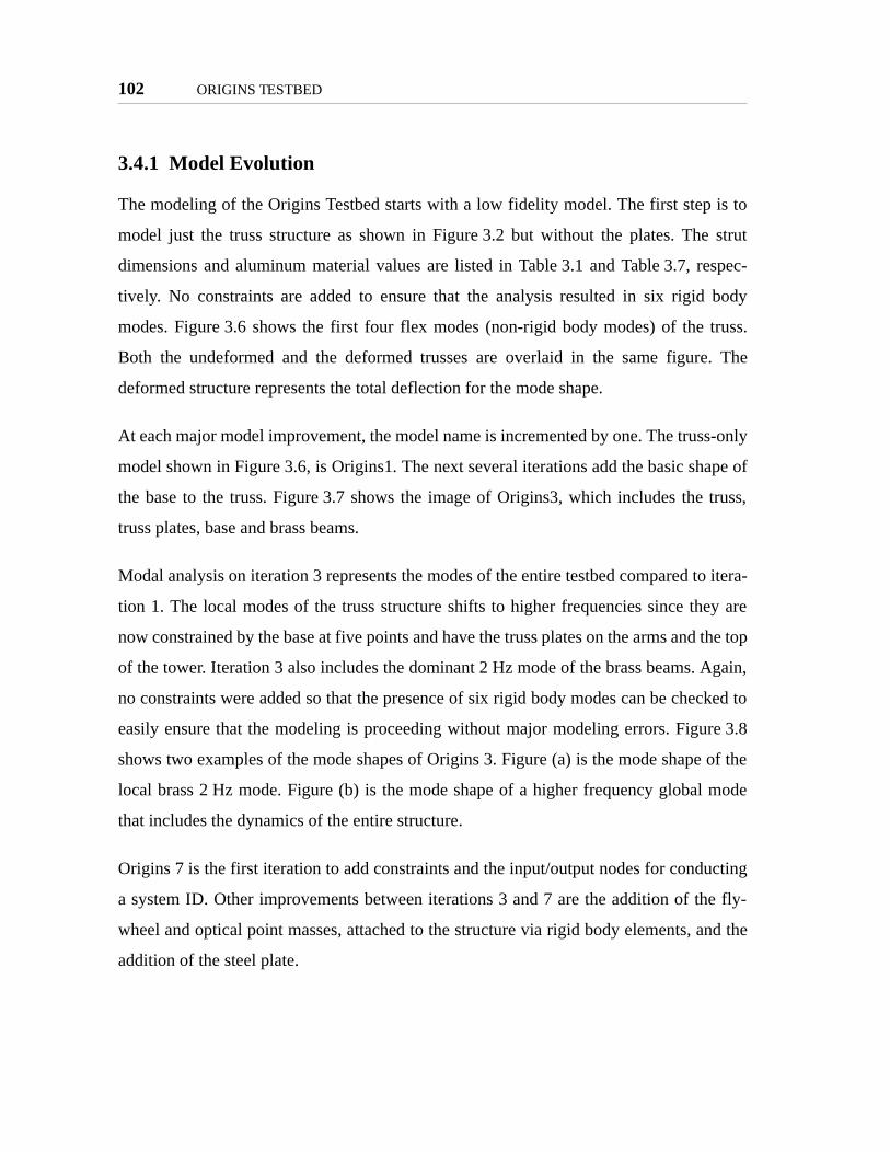
102 ORIGINS TESTBED
3.4.1 Model Evolution
The modeling of the Origins Testbed starts with a low fidelity model. The first step is to
model just the truss structure as shown in Figure 3.2 but without the plates. The strut
dimensions and aluminum material values are listed in Table 3.1 and Table 3.7, respec-
tively. No constraints are added to ensure that the analysis resulted in six rigid body
modes. Figure 3.6 shows the first four flex modes (non-rigid body modes) of the truss.
Both the undeformed and the deformed trusses are overlaid in the same figure. The
deformed structure represents the total deflection for the mode shape.
At each major model improvement, the model name is incremented by one. The truss-only
model shown in Figure 3.6, is Origins1. The next several iterations add the basic shape of
the base to the truss. Figure 3.7 shows the image of Origins3, which includes the truss,
truss plates, base and brass beams.
Modal analysis on iteration 3 represents the modes of the entire testbed compared to itera-
tion 1. The local modes of the truss structure shifts to higher frequencies since they are
now constrained by the base at five points and have the truss plates on the arms and the top
of the tower. Iteration 3 also includes the dominant 2 Hz mode of the brass beams. Again,
no constraints were added so that the presence of six rigid body modes can be checked to
easily ensure that the modeling is proceeding without major modeling errors. Figure 3.8
shows two examples of the mode shapes of Origins 3. Figure (a) is the mode shape of the
local brass 2 Hz mode. Figure (b) is the mode shape of a higher frequency global mode
that includes the dynamics of the entire structure.
Origins 7 is the first iteration to add constraints and the input/output nodes for conducting
a system ID. Other improvements between iterations 3 and 7 are the addition of the fly-
wheel and optical point masses, attached to the structure via rigid body elements, and the
addition of the steel plate.

Modeling the Origins Testbed 103
The rotation axis on the testbed is along the x axis, perpendicular to the longitudinal axis
of the brass appendages. The gimbal is located underneath the top base plate and weight of
the testbed is supported at three points along the axis of rotation: at each side plate and by
the gimbal in the center. These supports are modeled as nodes which are constrained in all
degrees of freedom except for the rotation about the x axis. Two of the nodes coincide
with nodes of the side plate elements, but the node in the center, representing the gimbal,
is not associated with any structural element in the model. It is attached to the structure via
48.9 Hz 49.2 Hz
66.5 Hz 74.8 HzFigure 3.6 Truss only

104 ORIGINS TESTBED
a rigid body element connected to the top of the base. Figure 3.9 shows a schematic of the
constraint locations.
The iterations between 7 and 11 are detailed improvements and do not involve any major
changes in assumptions, but mainly parameter values or meshing. The truss member ele-
ments are changed from rods to bars in order to refine the truss mesh from one element per
member to two. The counterweight masses are added below the steel plate. The property
values of the truss members and brass appendages are updated from the initial table values
to values calculated in previous experiments. A number of corrections are made, such as
the location of the steel plate below the base, the geometry of the truss tower, and the def-
inition of the beam orientation vectors.
Figure 3.7 Computer image of Origins Testbed - iteration 3
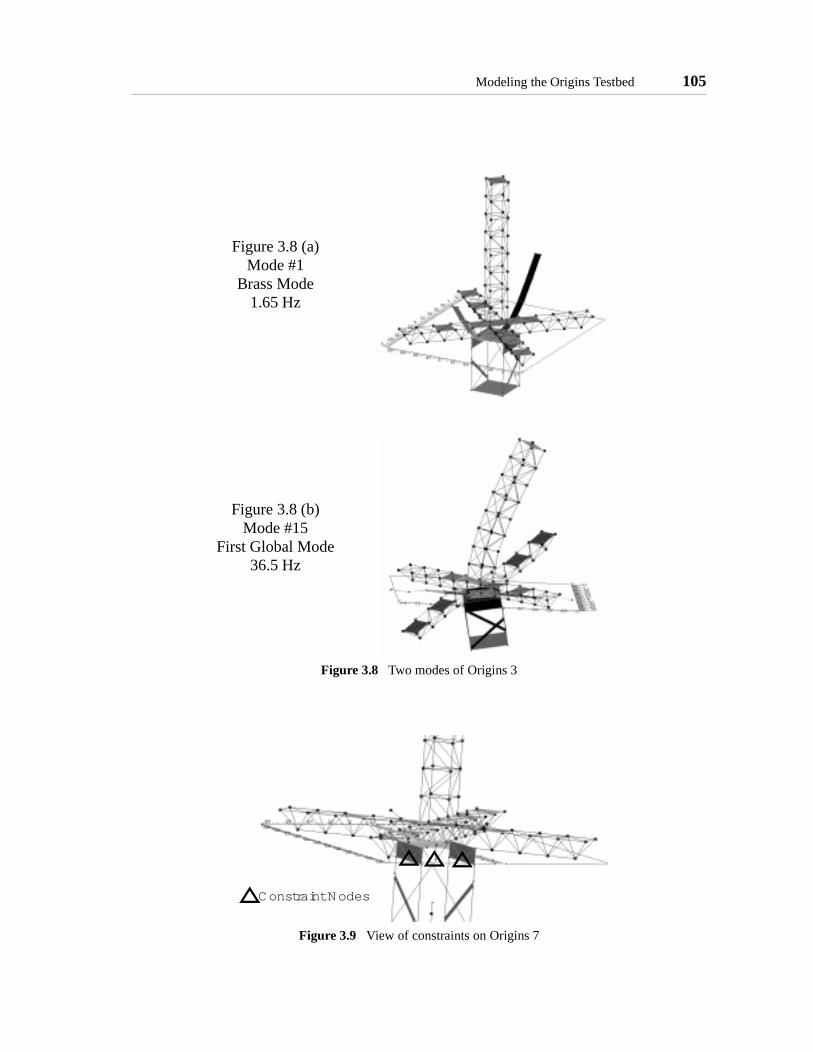
Modeling the Origins Testbed 105
Figure 3.8 (a)Mode #1
Brass Mode1.65 Hz
Figure 3.8 (b)Mode #15
First Global Mode36.5 Hz
Figure 3.8 Two modes of Origins 3
Figure 3.9 View of constraints on Origins 7
Constraint Nodes

106 ORIGINS TESTBED
The modes of Origins 11 are listed in Table 3.8. There is one rigid body mode left after
constraining the testbed in the x-rotational degree of freedom. The first four flex modes
are local modes of the brass appendages. The first global mode of the testbed is mode six
at 14 Hz. This mode and two other representative mode shapes of OT version 11 are
shown in Figure 3.10.
3.4.2 System Identification
A SYS ID was performed on the Origins Testbed by Olivier de Weck and Gregory Mal-
lory in summer of 2000 (Figure 3.11). The inputs are unit intensity white noise entered at
the reaction wheel and at the gimbal. The white noise is simulated by means of randomly
generating the voltage driving the reaction wheel motors and the gimbal motors. There are
three outputs from the system. The first is the angular displacement of the testbed mea-
TABLE 3.8 Origins 11 Modes
Frequency
Mode # Description [rad/s] [Hz]
1 RBM
2 Brass 11.3 1.81
3 " 11.7 1.87
4 " 69.4 11.0
5 " 69.5 11.1
6 Global 87.8 14.0
7 " 125 19.9
8 Brass 125 19.9
9 " 125 19.9
10 Global 148 23.6
11 " 155 24.7
12 " 183 29.2
13 " 184 29.4
14 Brass 190 30.3
15 " 190 30.3

Modeling the Origins Testbed 107
Figure 3.10 (a)Mode #6
First Global Mode(non-brass mode)
truss rocking about x-axis14.0 Hz
Figure 3.10 (b)Mode # 11
truss arm twisting 24.7 Hz
Figure 3.10 (c)Mode #19
truss tower and arms bending42.2 Hz
Figure 3.10 Origins 11 Mode Shapes

108 ORIGINS TESTBED
sured by angle encoder located at the gimbal node. The second output is angular velocity
of the testbed measured by the rate gyro, which is mounted on top of the reaction wheel
axial tube. The third output is the differential path length (DPL) of the internal laser
metrology system.
The transfer functions of the experimental data are shown in Figure 3.11. The light, noisier
curve is the experimental data and the smoother, dark curve is the measurement model.
The x-axis is the frequency in Hz and the y-axis is the magnitude in dB. An initial look at
the information from the transfer functions shows a prominent 2 Hz mode in all 6 input-
Figure 3.11 System Identification of the Origins Testbed - Experimental Data
10-2
100
102
-100
-50
0
Gim
bal -
> E
NC
10-2
100
102
-100
-50
0
50
Whe
el -
> E
NC
10-2
100
102
-60
-40
-20
0
20
Gim
bal -
> G
yro
10-2
100
102
-50
0
50W
heel
->
Gyr
o
10-2
100
102
-80
-60
-40
-20
Gim
bal -
> D
PL
10-2
100
102
-80
-60
-40
-20
0
Whe
el -
> D
PL
datafit
Frequency [Hz]
Magnitude [dB]
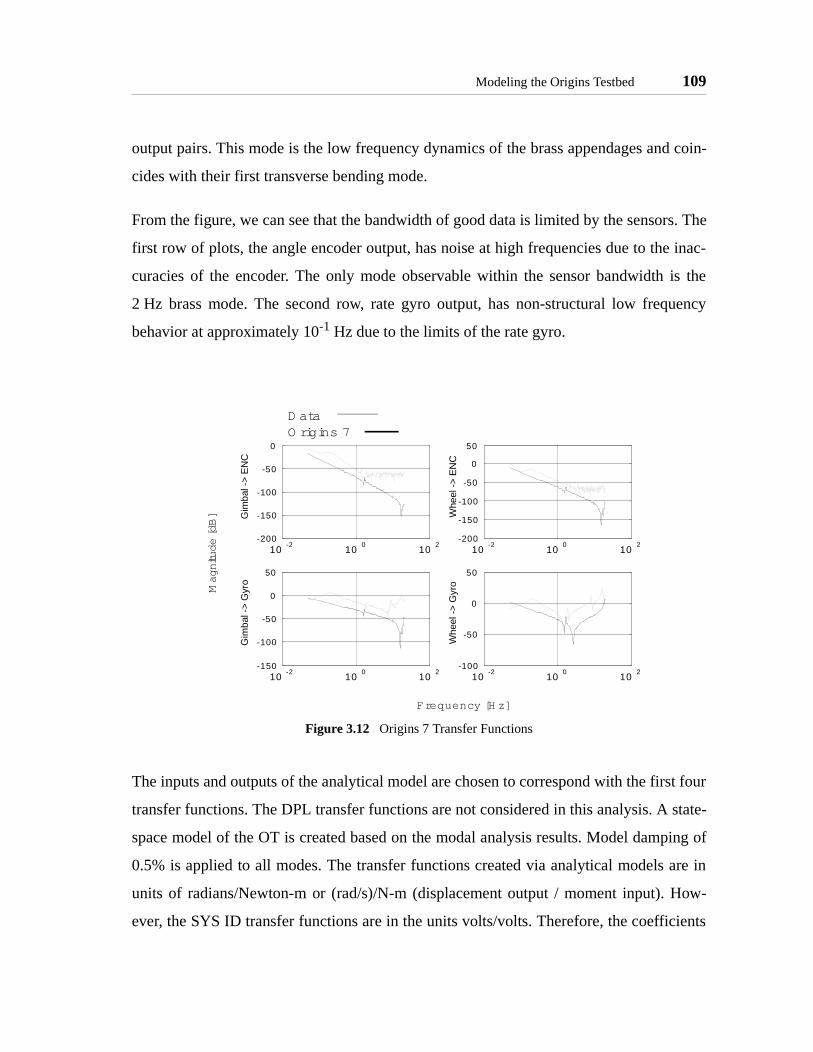
Modeling the Origins Testbed 109
output pairs. This mode is the low frequency dynamics of the brass appendages and coin-
cides with their first transverse bending mode.
From the figure, we can see that the bandwidth of good data is limited by the sensors. The
first row of plots, the angle encoder output, has noise at high frequencies due to the inac-
curacies of the encoder. The only mode observable within the sensor bandwidth is the
2 Hz brass mode. The second row, rate gyro output, has non-structural low frequency
behavior at approximately 10-1 Hz due to the limits of the rate gyro.
The inputs and outputs of the analytical model are chosen to correspond with the first four
transfer functions. The DPL transfer functions are not considered in this analysis. A state-
space model of the OT is created based on the modal analysis results. Model damping of
0.5% is applied to all modes. The transfer functions created via analytical models are in
units of radians/Newton-m or (rad/s)/N-m (displacement output / moment input). How-
ever, the SYS ID transfer functions are in the units volts/volts. Therefore, the coefficients
Figure 3.12 Origins 7 Transfer Functions
10-2
100
102
-200
-150
-100
-50
0
Gim
bal -
> E
NC
10-2
100
102
-200
-150
-100
-50
0
50W
heel
->
EN
C
10-2
100
102
-150
-100
-50
0
50
Gim
bal -
> G
yro
10-2
100
102
-100
-50
0
50
Whe
el -
> G
yro
D ataO rigins 7
Frequency [H z]
Magnitude [dB]

110 ORIGINS TESTBED
entered in the performance matrix, C, unit conversion factors. The resulting transfer func-
tions for Origins 7 are shown along with the SYS IS data in Figure 3.12.
The 2 Hz brass mode is visible in the model although the numerical value of the natural
frequency is slightly low. The general shape of the transfer functions resemble the experi-
mental data except at the limits of the angle encoder data. All four plots show a discrep-
ancy in the gain of the analytical model from the experimental data. The comparison of the
two transfer functions with the gyro as the output show that the model is missing several
poles and zeros.
Figure 3.13 shows the transfer functions of OT version 11. The gain of the two angle
encoder transfer functions are improved from version 7, and overlay the experimental data
more closely. The gain is still off from the gyro transfer functions and may be due to inac-
curate conversion factors. The poles and zeros missing from the wheel-gyro transfer func-
tion in version 7 appears in version 11, with the exception of one zero after the 2 Hz mode.
3.5 Summary
Table 3.9 lists an overview of all the improvements made on the Origins Testbed through-
out the model updating. Though the testbed has been updated significantly from the initial
truss-only model, it still requires more updating to be considered an accurate representa-
tion of the Origins Testbed dynamics. The analogy of the model updating procedure to the
model fidelity evolution still holds without a completed analytical model.
Although the Origins Testbed is complete, there are modeling errors in the analytical
model. The errors in the OT model are from both incorrect assumptions and parameter
errors. Although the Origins 11 model does not match the system identification data as
closely as desired, it is a relatively high fidelity model and is more accurate than a model
based on an incomplete design. The slopes of the transfer functions and the calculation of
the fundamental modes are more accurate than for a low maturity design. The stage of the
origins model is akin to the rod truss or low mesh bar truss of the sample problem.

Summary 111
Figure 3.13 System ID of Origins version 11
10-2
100
102
-200
-150
-100
-50
0
Gim
bal -
> E
NC
10-2
100
102
-150
-100
-50
0
50
Whe
el -
> E
NC
10-2
100
102
-150
-100
-50
0
50
Gim
bal -
> G
yro
10-2
100
102
-150
-100
-50
0
50
Whe
el -
> G
yro
DataO rigins 11
Frequency [Hz]
Magnitude [dB]

112 ORIGINS TESTBED
TABLE 3.9 Overview of Origins Model Evolution via Engineering Insight
Model Version Updates
1 truss only
2 add base plates and truss nodal masses
3 add base beams and truss plates
4 add flywheel mass, increase mesh of brass beams
5 add optical point masses: LASER, CCD, and minishaker
6 add steel plate
7 add constraint nodes, input/output nodes and constraints
8 change truss members from rods to barscorrected tower truss geometry
9 added counter-weight point masses, added steel screw (one was missing), updated brass properties from previ-
ous analysis of brass, updated strut properties from previ-ous analysis of struts, refine mesh of brass, base and truss plates, corrected truss nodal masses, corrected the loca-
tion of the steel plate
10 refined truss plate geometry, redefined rigid body ele-ments
11 correct bar orientation vectors, refine truss member mesh

Chapter 4
ARGOS
The ARGOS (Active Reconnaissance Golay-3 Optical Satellite) testbed is a ground based
testbed designed to demonstrate modular Golay-3 technology. It is the project of an under-
graduate design class called CDIO (Conceive, Design, Implement, Operate) and is sched-
uled for completion by the end of the spring term of 2002. Although the multiple aperture
array technology concept has been demonstrated by observatories such as the Large Bin-
ocular Telescope (LBT), the contribution that ARGOS provides to the field is in its modu-
lar design and implementation of fizeau beam-combining on a rotating inertial frame.
Currently, the goal of ARGOS is to image the International Space Station (ISS) while
ARGOS is slewing. If this main objective is not completed, however, there are lower lev-
els of mission success criteria as shown in Table 4.1.
TABLE 4.1 Mission Success Criteria (from PDR)
Level of Success Criteria 1 Criteria 2 Criteria 3Minimum Slew while keeping
moving object in FOVIncoherent imaging Image of a celestial
object of known fea-ture scaleFull Slew while keeping ISS
in FOVCoherent imaging
113

114 ARGOS
4.1 Description of ARGOS
The following description of ARGOS contains an overview of the subsystems relevant to
its structural design and a description of the frozen design iteration for the disturbance
analysis to follow in the next section. The information on the subsystem designs are based
primarily on the Preliminary Design Review (PDR) of May 2001 [CDIO, 2001], with the
exception of a few key subsystem design changes that have taken place since PDR.
4.1.1 Architecture
ARGOS is a ground based testbed that resembles the behavior of a space based system. As
such, most of the design decisions are made as though the testbed will be space-borne to
demonstrate flight capabilities of the design concept. However, certain key design features
are modified in order for the testbed to function on ground. The first important difference
between the two environments is gravity. The space based design does not have to support
its weight nor deal with the offset between the center of gravity and the center of rotation.
The second important constraint is the time and cost constraint of the CDIO environment.
The testbed, to be completed by the end of spring 2002, will be less redundant and simpler
than a true space telescope.
The ideal architecture for the space based system is a single function distributed system.
The telescope is divided into three subapertures, each holding one collector telescope, and
a combiner module. The combiner module is what the subapertures dock to and where
they send their light for combining. Each of the three subapertures has its own fully inde-
pendent bus with modular subsystems (power, computer, RWA, etc.) to allow separate
launches and independent docking to the center bus.
The ground system architecture is modified from the space system and is a single-function
monolithic design, where monolithic refers to the subsystem functions. All subsystems are
modularized for simple interfaces, but complete subsystems are not placed in all three sub-
apertures. All three subapertures are required for the entire system to function because
Description of ARGOS 115
only one of each subsystem (such as computer, communications system, and reaction
wheel assembly) will be placed on the testbed. This simplification is justified because the
technological challenge and objective of ARGOS is the modularity of the optics not the
redundancy of subsystem. The modularity refers to the ability to remove and replace the
subapertures from the center bus and the ability to remove and replace the subsystems,
such as the batteries, computers and communications equipment.
4.1.2 Optics
This section describes the key components of the optical train and briefly discusses the
optical design. The optical design requirements are derived from the mission objectives.
In order to be able to image the ISS during its orbit, the passive optics must meet the fol-
lowing requirements:
1. 0.35 arc second angular resolution or better
2. Science light in the visual spectrum
3. less than l/10 wave error
4. greater than 0.65 encircled energy
5. greater than 4 minute field of view
6. greater than 0.03 second integration time
A commercial off-the-shelf telescope, the Takahashi Mewlon 210, serves as the subaper-
ture. It is a Dall-Kirkham type reflecting telescope with an elliptical primary mirror and
spherical secondary mirror. The main advantage of the Dall-Kirkham telescope is that
spherical aberration is eliminated. Spherical aberration causes the light to not focus at a
single point. Additionally, the telescope does not have a correcting lens at the entrance
and, therefore, most of the weight of the telescope is from the primary mirror at the base.
The lack of a correcting lens makes the Takahashi less heavy than a similar sized Schmidt-
Cassegrain telescope. The Takahashi-brand telescope is chosen primarily for its superior
surface accuracy. The important properties of the Takahashi are listed in Table 4.2.

116 ARGOS
The three Takahashi telescopes are configured into a Golay-3 configuration: 120 degrees
apart about a beam combiner in the center of the array. The radius of the circle through the
center of the subapertures is 19.185 cm. This configuration is necessary to achieve the
required 0.35 arcsecond angular resolution. The Golay-3 configuration is shown in
Figure 4.1.
Relay optics send the light from the subaperture to the beam combiner and include actua-
tors to compensate for errors in the light path (wavefront tilt, beam shear, optical path-
TABLE 4.2 Takahashi properties
Property Value
Weight 8 kg
Effective Aperture 210 mm
Primary Mirror 220 mm f/4
Secondary Mirror 65 mm f/2.9
Tube Diameter 244 mm
Tube Length 700 mm
Figure 4.1 Golay-3 configuration
Beam Combiner
SubAperture
6.985 cm
19.185 cm
31.385 cm

Description of ARGOS 117
length difference) The elements of the optical train usually include a collimator, fold
mirror, optical delay line, and fast steering mirror. The layout of the relay optics for
ARGOS is illustrated in Figure 4.2; the elements of the optical train are numbered in
order, 1-8, and the dimensions shown are in mm. Table 4.3 lists the relay optics and the
displacement between them. The displacements listed for optic n are from the center of
optic n-1 to the center of optic n. The only exception is the displacement listed from the
collimator to the first fold mirror.
The collimator is the only refractive optic used in the telescope. It converts the focusing
light exiting the Takahashi telescope into collimated light with a diameter of 21 mm. The
collimator is placed within and supported by the Takahashi telescope. The fold mirror,
delay line and fast steering mirror are flat mirrors actuated by PZTs and voicecoils to con-
trol the optical path to compensate for jitter in the structure. The first three fold mirrors are
placed under the Takahashi on an optics bench. The light from the optics bench is then
sent from the telescope to the center bus, which holds the last fold mirror, the beam com-
biner and the CCD.
TABLE 4.3 Relay Opticsa
a. The displacements listed are the distance between the bottom of the telescope to the first fold mirror.
# Optic ∆x [mm] ∆z [mm]
1 Collimator n/a n/a
2 Fold Mirror 1 0 -70.0
3 Fold Mirror 2 -70.0 0
4 Fold Mirror 3 0 35.0
5 Fold Mirror 4 242.7 0
6 Beam Combiner Primary
19.2 -95.0
7 Beam Combiner Secondary
0 75.0
8 CCD 0 86.0

118 ARGOS
The beam combiner is sized to obtain the desired 1:10 compression ratio. The beams strik-
ing the surface of the combiner primary mirror must have the same configuration as the
Golay-3 subaperture configuration, at 1/10th scale. To obtain this degree of compression,
the minimum optical radius of the primary mirror of the beam combiner must be 29.685
mm. The important dimensions of the beam combiner are listed in Table 4.4.
Figure 4.2 Relay Optics Schematic - dimensions in mm
TABLE 4.4 Beam Combiner
Parameter Value
Diameter of single beam 21 mm
Center of beam to center of beam 33.2 mm
Minimum optical radius of combiner 29.685 mm
1
23
4 5
6
7
8
35.070.0
70.0
242.7
19.2
11.0
75.0
20.0
x
z

Description of ARGOS 119
The CCD camera collects the combined science light for imaging the science target. The
field of view requirements determine the size of the CCD. Other requirements, such as the
speed of data output, determine the quality of CCD necessary. These other requirements
affect the ability for ARGOS to capture the ISS while slewing, but does not affect the
structural design. The PDR choice of CCD is the Apogee AP10, which has dimensions of
177.8 x 177.8 x 76.2 mm
4.1.3 Attitude Control System
The sensors and computers on ARGOS must be able to determine the orientation of
ARGOS with respect to the earth, and then find and slew to the science target autono-
mously. The ability to slew to the target in an inertial reference frame is one of the main
features of ARGOS that sets it apart from other current sparse aperture observatories.
Slewing is achieved by mounting the testbed on an air bearing and using reaction wheels
to provide attitude control.
The air bearing works by blowing air under the object that it supports, which lifts the
object enough to prevent contact with the air bearing stand. The mass of ARGOS is lim-
ited to 26 kg by the weight capacity of the air bearing. The layout of the optics in the cen-
ter bus is constrained by the presence of the air bearing at the center of the structure.
Figure 4.2 shows that the subaperture optics are all above the plane of the CCD. The CCD
must be mounted above the air bearing and thus above the center of rotation. The rest of
the optics are then also above the center of rotation. The weight of the optics must be
countered by placing weight below the airbearing. Therefore, the subsystems will be
placed below the optics. However, when ARGOS tilts, the air bearing stand must be able
to clear any structure placed below the center of rotation.
The torque authority of the RWA on ARGOS is required about three axes. The sizing of
the RWA depends upon the inertia of the structure and the desired slew rate. The RWA is
expected to contribute significantly to the total mass of ARGOS and since the total weight
that the air bearing can support is limited, the final design must minimize the size of the

120 ARGOS
RWA. The rotational inertia of the system is divided into two components: the inertia
about the principal axes (the center of gravity) and the displacement of the center of grav-
ity from the center of rotation (parallel axis). Minimizing the inertia about the principal
axes is done by keeping the massive subsystems as close to the center of rotation as possi-
ble. To reduce the second component of inertia (from the parallel axis theorem) to zero,
the center of gravity (CG) and the center of rotation must be at the same point. However,
manufacturing tolerances in the structural material and inability to distribute the weight of
the subsystems (computers, batteries, GPS receiver, etc.) limit how close these two points
can be placed passively. The requirement on the structural design is to get position the CG
within a 1 mm radius of the center of rotation. The separation is reduced further through
an active balancing system.
4.1.4 Structure
The structure is designed to support the optical train, to hold the subsystems together, and
to isolate the optics from the disturbance. The primary disturbance is the vibrational noise
from the RWA, but the optics are also sensitive to heat from the electrical components.
The structure must also meet the modularity requirement that, like the inertial reference
frame, sets ARGOS apart from other current observatories.
Figure 4.3, Figure 4.4, and Figure 4.5 show the structural design of ARGOS as of the
PDR. The telescope collar is the mount that supports the Takahashi. The component cage
supports the subsystems and is designed such that the subsystems can be arranged on a
rack that easily slides on and off the cage. The optics bench supports the first three fold
mirrors of the optical train. The center bus holds the fourth folding mirror, the beam com-
biner and CCD camera. The center bus is also the attachment point between the structure
and the air bearing.
Figure 4.4 illustrates the clearance of the air bearing between the component cages. The
air bearing stand must be able to clear the structure so that ARGOS can tilt in a full 60
degree cone off vertical. This clearance requirement caused the design to have the cages
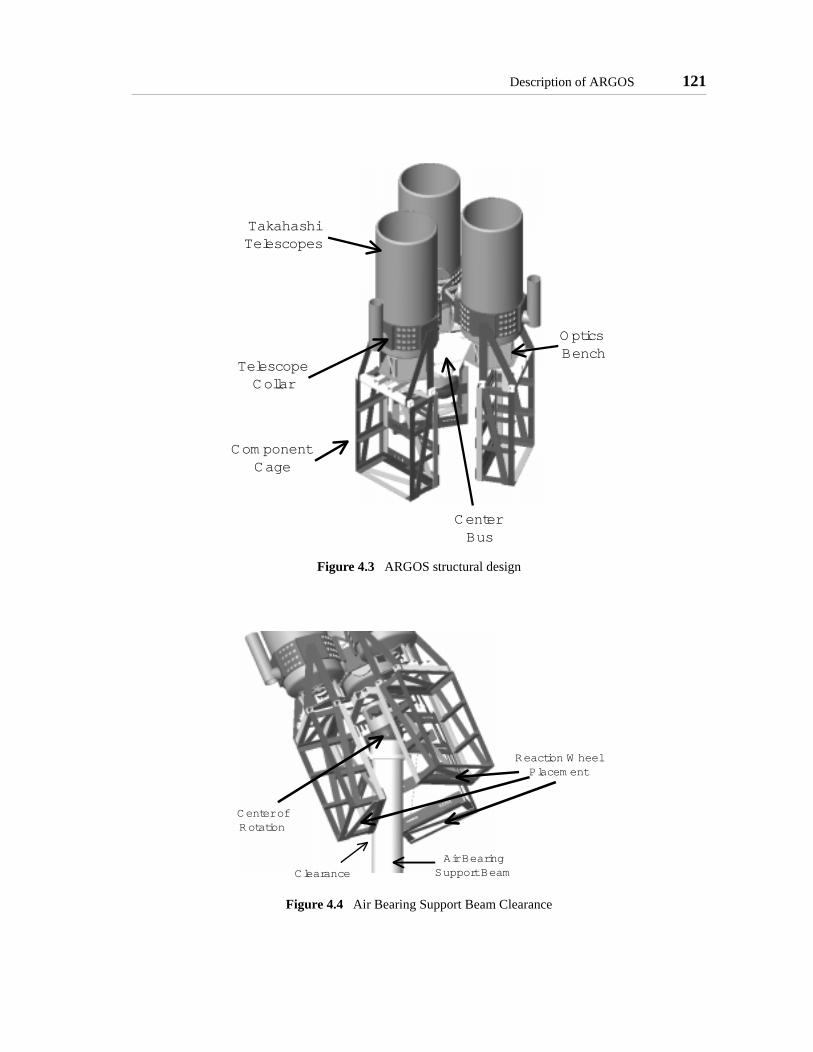
Description of ARGOS 121
Figure 4.3 ARGOS structural design
Figure 4.4 Air Bearing Support Beam Clearance
Com ponent Cage
TakahashiTelescopes
O ptics Bench
Center Bus
TelescopeCollar
Air BearingSupport Beam
Center ofRotation
Clearance
Reaction W heelPlacem ent

122 ARGOS
ope is
ht bear-
bus. The
own in
placed radially outward from the center of rotation. The RWA assembly is distributed
among the three subapertures. One wheel will be placed on the bottom rack of each cage
for three wheels total.
Figure 4.5 shows the telescope collar without the Takahashi. The collar is designed to
interface with the Takahashi’s dove-tail collar mount so that the weight of the telesc
supported as recommended by the manufacturer. The support mounts are the weig
ing members of the subaperture design and connect the subapertures to the center
support beams side by side will add bending stiffness to reduce radial bending as sh
Figure 4.5 Telescope Collar
Figure 4.6 The three bending directions the support beams must counter
Support M ounts
Additional C onnection Point
C om ponentC age
Sag
Radial Bending
Twist
Subaperture
Center Bus
Subaperture
Center Bus

Description of ARGOS 123
t tilt,
more,
llar will
volves
Figure 4.6, which is the bending about the z-direction (z points vertically upwards). A sec-
ond set of support beams below the collar (not shown in Figure 4.5) will increase the
bending stiffness in the “sag” direction. The optical performance metrics (wavefron
OPD) are most sensitive to the sag direction. In order to increase the sag stiffness
another connection point for the subaperture has been added at the collar. Each co
connect to the other two above the center bus. Thus the assembly of ARGOS in
Figure 4.7 Side view of subaperture and center bus geometry
Center of Rotation
CCD Camera
80.
94
50.
136
462
75
358
OpticalTrain

124 ARGOS
sliding the subaperture and collar together via the support beams, tightening the support
beams with a screw, and pinning the collar connection points together.
Figure 4.7 shows the side view of one subaperture and the center bus. The figure illus-
trates how the optical train fits into the design.
Table 4.5 lists the principal dimensions of the structure. The Golay-3 layout of the tele-
scopes (Figure 4.1) is used to determine the positions of the subapertures with respect to
the center bus. The vertical dimensions of the subaperture with respect to the center bus
are designed based on the optical train positions listed in Table 4.3.
4.2 ARGOS Integrated Model
ARGOS is currently between the preliminary design phase and the critical design phase
and thus all modelling is still low-fidelity. Though the architecture has been chosen, the
TABLE 4.5 Structural Dimensions
Dimension Value [mm]
Vertical distance between optical bench and bot-tom of Takahashi
95.
Vertical distance between center of collar and top pair of support beams
315
Horizontal distance between pair of support beams
50.
Vertical distance between support beam pairs 136.5
Vertical distance between center of collar and bot-tom of Takahashi
80.
Total height of center bus 358
Length of one side of center bus hexagonal optics plate
116
Height of component cage 462
Width of component cage 300.
Depth of component cage 150.

ARGOS Integrated Model 125
design of the subsystems are still evolving. The structural design is dependent upon the
other subsystems and must be kept versatile to accommodate refinement of subsystem
requirements as they become better defined during the design process. However, in order
to perform a disturbance analysis at this stage, a design iteration must be chosen for analy-
sis, i.e. frozen, at the design matures. The disturbance analysis at this early stage will
determine if the design is adequate or needs major improvements.
4.2.1 Structural Dynamics
Because ARGOS is in a low fidelity design stage, the analytical model created will be
analogous to the stick models of Chapter 2. For the stick model, only the main structural
components, input nodes and output nodes are needed. Figure 4.8 shows the finite element
model of the assembled structure and Figure 4.9 shows the details of one subaperture and
the center bus including the optics nodes and the reaction wheels.
Figure 4.8 Assembly
Center Bus
Reaction W heel
Subaperture 1 Subaperture 2
Subaperture 3
SubapertureOptics Plate
Center BusOptics Plates

126 ARGOS
The telescope and collar are modeled as a single rigid element connected the top of the
beams supporting the collar to each other. This simplification is made because the collar is
holding onto the telescope near the location of the primary mirror and the mirror is made
out of rigid glass material. The component cage is modeled in more detail using beams to
capture the geometry and plates to model the rack. The component cage is modeled in
detail since the reaction wheel disturbances are added to the system via the bottom rack.
The optical train is modeled by placing a node at the location of the center of each optical
component.
Figure 4.10 illustrates the total deformation of the first mode shape. The image shows that
the bending in the sagging direction is a fundamental mode.
Figure 4.9 Subaperture and Center Bus
C om ponent Cage
Telescope & Collar
SupportBeam s
CCD
Beam Com biner
First ThreeFold M irrors
Fourth FoldM irror (hidden)
Reaction W heel
Constraint Node123=xyz translations

ARGOS Integrated Model 127
4.2.2 Disturbance Model
Reaction wheels are expected to be the largest source of disturbances on ARGOS. RWA
spin at high speeds and may vibrate due to static and dynamic imbalances. These vibra-
tions can impinge on the structure causing undesired motion of the optical components.
Static imbalance is the offset of the center of gravity from the axis of rotation. It is mod-
eled as a small mass, ms, at distance, rs, that displaces the center of gravity from the center
of rotation along the radial direction (Figure 4.11(a)). The dynamic imbalance is the offset
of the principal axial axis from the axis of rotation. It is modeled as a pair of small masses,
md, at distance, rd, that are displaced in the z direction, one above the radial axis and one
below by distance, h (Figure 4.11(b)) [Bialke, 1997].
The ARGOS reaction wheels are not yet built, but are expected to have a vibration envi-
ronment similar to that of unbalanced, off-the-shelf professional wheels. Therefore, RWA
Figure 4.10 First Mode Shape [52.7 Hz]
Undeform edStructure
Deform edStructure

128 ARGOS
disturbance model used in the disturbance analysis is one based on vibration data taken
from an Ithaco B Wheel (model TW-16B32), by Orbital Sciences, in February and April
of 1997. The disturbance model was created by Masterson [Masterson, 1999].
The disturbance caused by the reaction wheels are expressed as a vector, m, of three forces
(one in the axial and two in the radial) and three moments (again, one in the axial and two
in the radial). From empirical analysis of reaction wheel test data, these disturbances have
been found to be tonal in nature occurring at certain harmonics of the wheel speed and
their amplitudes can be expressed as a function of the wheel speeds squared:
(4.1)
where m(t) is the disturbance, C is the amplitude coefficient, f is the wheel speed, h is the
harmonic number, φ is the phase, the subscript i indicates the wheel speed, and j indicates
the disturbance type. The disturbance type refers to whether the disturbance is a force or a
moment and if it is in the axial or radial directions. The harmonics and amplitude coeffi-
cients for the Ithaco B-Wheel are given in Table 4.6.
Figure 4.11(a) Static Imbalance Figure 4.11(b) Dynamic ImbalanceFigure 4.11 Reaction Wheel Imbalance Representation
ω
rs
m s
z
m d
m d
ω
z
rd
hh
mij t( ) Cjfi2
2πhjfit φij+( )sin=

ARGOS Integrated Model 129
Equation (4.1) models RWA disturbances at discrete wheel speeds. However, RWAs oper-
ate in a range of speeds. Melody developed a stochastic broadband model of the RWA dis-
turbances assuming that the wheel speed is a random variable [Melody, 1995]. The Power
Spectral Densities (PSDs) for the stochastic model of the B-wheel is shown as the dashed
lines in Figure 4.12. The state space model (solid lines) is fit to the broadband disturbance
PSDs for use in disturbance analysis.
Because the wheel is symmetric in the radial direction, the forces and moments in and
about the radial directions differ by only 90 degree phase and are combined. The moment
about the axial direction due to imbalances is considered to be negligible compared to the
total moment about the axial direction. Thus, in the wheel frame of reference, there are
only three types of disturbances, the radial force, radial moment and the axial force.
Recall that the disturbance state-space representation is given by equation (2.23), rewrit-
ten here:
TABLE 4.6 Ithaco B Wheel Model [Masterson, 1999]
Radial Force Radial Moment Axial Moment
h C [N/rpm2] h C [Nm/rpm2] h C [Nm/rpm2]
0.99 2.134 e-8 .99 6.305 e-9 0.99 7.27 e-9
1.99 5.10 e-9 1.99 1.314 e-9 1.41 4.97 e-9
2.46 6.09 e-9 3.16 8.89 e-10 2.82 9.75 e-9
3.16 7.83 e-9 4.56 2.609 e-9 5.95 1.9889 e-8
3.87 5.28 e-9 5.28 3.722 e-9
4.56 9.05 e-9 5.97 2.375 e-9
5.28 1.752 e-8 6.23 2.763 e-9
5.98 3.04 e-8 6.68 3.347 e-9
6.71 2.053 e-8 7.38 4.767 e-9
8.09 3.246 e-8 8.09 4.005 e-9
8.83 3.517 e-8 8.80
9.54 2.991 e-8
10.25 3.138 e-8

130 ARGOS
ion:
o Guti-
wheel
(4.2)
where the superscript, w, indicates that the model is in the wheel reference frame
(Figure 4.12). The disturbances, ww, correspond to the reaction wheel disturbances, ww,
must be converted to the spacecraft frame before being inputted as plant disturbances.
Equation (2.22) rewritten here from Chapter 2, is the plant’s state-space representat
(4.3)
where the superscript, s/c, indicates the disturbance in the spacecraft frame. Homer
errez developed methods to transfer the reaction wheel disturbance models from the
Figure 4.12 B-Wheel Disturbance PSD’s in Wheel Frame
100
101
102
103
10-10
10-8
10-6
10-4
10-2
Em pirical M odel PSDRadial ForceAxial ForceRadial Torque
State Space PSDRadial ForceAxial ForceRadial Torque
Frequency [Hz]
RW Disturbance PSD
qd· Adqd Bdd+=
ww
Cdqd=
qp· Apqp Bw ws/c+=
z Czqp=

ARGOS Integrated Model 131
egrees
tward
in the
fferent
e
heels.
frame to the spacecraft frame [Gutierrez, 1999]. The attitude of the reaction wheels are
defined using Euler angles as defined in Figure 4.13.
The first rotation, β, is about the wheel’s original z axis. The second rotation, θ, is about
the wheel’s new y axis after the first rotation. The third rotation, γ, is about the wheel’s
new x axis after the second rotation. The wheels on ARGOS are arranged 120 d
about the center and angled 45 degrees down from the vertical pointing radially ou
(angled 45 degrees up towards the center) as shown in Figure 4.14.
The combination of the three angles are non-unique since the wheels are symmetric
radial direction. The orientation angles are chosen such that the only angle that is di
between the three wheels is β, the rotation about z, and such that the third rotation, γ, is
zero. The angles for the three wheels are β1 = 270, β2 = 30, β3 = 150, θ = 135, γ = 0.
The position of the wheels are given by vector wr. The elements of r correspond to th
position of the spacecraft CG from the wheel’s CG and are the same for all three w
The position vector for all three wheels are:
(4.4)
Figure 4.13 Euler Angles (s/c denotes spacecraft frame; w denotes wheel frame) [Gutierrez, 1999]
zw
zs/c
yw ys/c
xwxs/c
0
0
0
β
θ
γ
yw/
yw0
xw0
xw/
yw/
xw/
xw// xw
zw0 zw
/
zw//
zw//
zw/// zw
///
yw//
yw yw
,
,
,,
,
1st Rotation 2nd Rotation 3rd Rotation
rw
0.044– 0.000 0.420–T
=

132 ARGOS
The Euler angles and the position vector are used to calculate a transformation matrix, T,
such that Equations (4.2) and (4.3) can be combined to give the following equation for the
appended plant and disturbance state-space system:
(4.5)
4.2.3 Optical Sensitivity
The performance for ARGOS is the optical path length difference (OPD) of the light trav-
eling through two different subapertures to the CCD camera. If the path length of light
Figure 4.14 Reaction wheel orientation
TABLE 4.7 ARGOS wheel Euler angles
Wheel # β θ γ1 270 135 0
2 30 135 0
3 150 135 0
zw1 zw2
xs/c
zs/c
120°
45 °
45 °xw1
yw1
xw2
yw2
q·Ad 0
BwTCd Ap
qBd
0d+=
z 0 Czq=

ARGOS Integrated Model 133
traveling through the subapertures are termed OPL1, OPL2 and OPL3, then there are three
possible OPDs to calculate:
(4.6)
However, there are only two unique OPDs to calculate since the third equation is a linear
combination of the first two:
(4.7)
To get the optical path length difference, first the optical path length of one subaperture
must be calculated. The OPL is calculated by summing the distances the light travels
between elements in the optical train. However, it is necessary to calculate the OPL as a
function of mirror translations and rotations. The calculation can easily be used for the
other two subaperture OPLs by simply changing the element nodes and rotating the sensi-
tivities since they are dependent upon the degrees of freedom with respect to the space-
craft frame.
Assuming small displacements, the OPL is calculated as a function of the nodal displace-
ments using finite differences. The first step is to calculating the nominal OPL for the opti-
cal train. The next step is then to perturb one degree of freedom by a known amount and
calculate the new OPL. This step is iterated through all the degrees of freedom throughout
the optical train. A linear sensitivity is assumed such that the change in the ODL is given
by:
(4.8)
OPD12 OPL1 OPL2–=
OPD23 OPL2 OPL3–=
OPD13 OPL1 OPL3–=
OPD13 OPD12 OPD23+=
OPL1 OPL2–( ) OPL2 OPL3–( )+=
OPL1 OPL3–=
∆OPLOPLi OPL0–
∆xi----------------------------------
∆xi
i 1=
n
∑=

134 ARGOS
where the quantity within the parentheses is the sensitivity of the ith degree of freedom.
Figure 4.15 shows an example of a sensitivity calculation. The light enters at node a and
bounces off two flat mirrors (b and c) at 45 degree angles and exits at d. The nominal path-
length is shown by the dotted lines and the new pathlength is shown by the solid line.
The pathlengths for the example are given by the following equations:
(4.9)
Because the mirrors at b and c are nominally at 45 degrees to the light path, dx1, dy2 and
dx3 are all equal to ∆yb. The difference and sensitivity are then calculated to be:
(4.10)
The optical sensitivity matrix for ARGOS was conducted in a similar fashion, yet with the
assistance of a software code developed by Masterson [Masterson, 2000]. The code
Figure 4.15 Example calculation of optical path length sensitivity
L1
L2
L3 - dx3
L2+ dy2
dy2
dx3
L3
L1 - dx1 dx1
∆ybnode: a b
cd
b
OPL0 L1 L2 L3+ +=
OPL∆ybL1 dx1–( ) L2 dy2+( ) L3 dx3–( )+ +=
∆OPD∆yb∆yb–=
∆OPD∆yb
∆yb----------------------- 1–=

Disturbance Analysis 135
requires the geometrical layout of the optical train, the prescription of each optic and the
incident ray direction (Figure 4.16).
4.3 Disturbance Analysis
The A,B,C,D state-space matrices are created for the structure and the disturbances. The A
matrix is created from the structural dynamics of the system. The B matrix is the distur-
bance input matrix denoting where the reaction wheel noise enters the system. The C
matrix is created from the optical sensitivities.
The PSD of the disturbance to performance behavior of ARGOS is the bottom figure in
Figure 4.17. The methods to calculate the plots are from Gutierrez [Gutierrez, 1999]. The
area under the PSD curve is the RMS of the performance. The cumulative RMS plot above
the PSD is the integral of the PSD as a function of the frequency. The large jumps in the
cumulative RMS curve indicate modes that contribute significantly to the total RMS.
Table 4.8 lists the modal frequencies corresponding to the jumps in OPD1 and OPD2;
these are approximate values taken empirically from the cumulative RMS plot.
Figure 4.16 Ray trace for sensitivity calculation
-100 -50 0 50 100 150 200-80
-60
-40
-20
0
20
40
60
80
8
7
6
5
Y
2
1
4
3Z

136 ARGOS
The analysis of the low fidelity stick model in the sample problem showed that the overall
modal behavior, such as the mode shape and the slope of the PSD, are similar to the truth
model. However, the natural frequencies are not of the same order of magnitude of the
Figure 4.17 PSD and cumulative RMS for ARGOS
Frequency [Hz]
cumulative rms
m
101
102
103
104
10-10
10-8
10-6
10-4
10-2
100
PSD
OPD1OPD2
[m2/Hz]
10 1 102 10 3 10 40
0.04
0.08
0.12
0.16
OPD1
OPD2
0.1280 m
0.1546 m

Disturbance Analysis 137
truth model. For a higher fidelity stick model, the natural frequencies are of the same order
of magnitude as those for the truth model.
The finite element model of ARGOS is considered to be a low fidelity stick model. It is
the first model to be created for disturbance analysis with many assumptions for simplifi-
cation. As such, the RMS values calculated from the PSD of the ARGOS stick model only
indicate the order of magnitude of the OPD. The results obtained indicate that the structure
must be stiffened to meet requirements. The mode shapes can be used to determine critical
locations for redesign.
For example, the 52 Hz mode corresponds to the first mode of the system shown in
Figure 4.10. This is a critical mode for both OPD metrics and is the most significant con-
tributor to OPD2. This result indicates that the bending of ARGOS subsystems in the sag
direction is the most flexible of the three bending stiffnesses shown in Figure 4.6. The
actual values calculated for OPD1 RMS and OPD2 RMS are 0.12 m and 0.15 m.
Two more mode shapes are shown in Figure 4.18, corresponding to the critical modes at
95 Hz and 97 Hz. Mode #13 is in the twist bending direction and its contribution to the
OPD indicates that ARGOS should be stiffened in this direction. One solution is the addi-
tion of another beam or beams perpendicular to the support beams to hold them together.
Mode #14 is the local plate mode of the rack holding the reaction wheels. The plate and
the component cage beams are not stiff enough to isolate the RWA disturbances from the
rest of the structure.
TABLE 4.8 Critical Modes
Natural Frequencies [Hz]
OPD1 OPD2
52 52
67 97
95 122
164 179

138 ARGOS
4.4 Summary
A first run disturbance analysis of ARGOS indicates that the structure as it currently is
designed, is not stiff enough to isolate the optical elements from the disturbances of the
reaction wheels. The numerical results of the analysis are indicators of the order of magni-
tude of the OPD. The critical modes determined through the cumulative RMS plots and
their corresponding mode shapes determine where the structural design of ARGOS must
be improved. The structural model of ARGOS created to run the analysis is a low fidelity
model that will require more refinement as the design matures.
Figure 4.18(a) Mode #13 [95.9 Hz] Figure 4.18(b) Mode #14 [98.8 Hz]Figure 4.18 High frequency mode shapes for ARGOS

Chapter 5
CONCLUSION
odel,
that is
are the
pro-
5.1 Summary
Space telescopes are large, deployable flexible structures that operate in a disturbance
environment. To meet their performance requirements, they must demonstrate high stabil-
ity and pointing accuracy. The size of space telescopes and their 0-g design inhibit full-
scale testing on the ground; therefore, accurate models are necessary to predict their per-
formances.
The accuracy of the performance predictions depends upon the level of fidelity of the
model. Model fidelity is dependent upon design maturity and model updating. A truss
sample problem in Chapter 2 is used to describe the different stages of model fidelity. The
design maturity is simulated by different finite element types: (listed in order of increasing
fidelity) a Bernoulli-Euler beam, a Timoshenko beam, a truss with rod elements and a
truss with bending beam elements. Model updating is simulated by meshing the finite ele-
ments at different degrees of refinement. The models are compared to a “truth” m
which is the highly refined truss with bending elements.
Chapter 3 presents the Origins Testbed (OT) as an example of a mature model
based upon a structure which has been built. Experimental data is available to comp
analytical model transfer functions to assess the fidelity of the analytical model. The
139

140 CONCLUSION
cess of modeling the OT is used as an analogy of the evolution of model fidelity due to
design maturity.
Chapter 4 presents the ARGOS testbed as an example of a low fidelity model at a low
design maturity level. Though the design of ARGOS is still being changed, one iteration is
fixed in order to complete a disturbance analysis. The disturbance analysis requires the
development of a reaction wheel disturbance model using Ithaco B-wheels as the distur-
bance source for ARGOS. Additionally, a sensitivity matrix for the optical train is devel-
oped to calculate the performances. The disturbance analysis results are examined based
upon the knowledge gained from the sample problem. Only the order of magnitude of the
resulting OPD is considered, which indicates that the design of the structure of ARGOS
requires significant improvements. The cumulative RMS plot indicates the modes that
contribute significantly to the total RMS. The numerical values of the natural frequencies
are not significant for low fidelity models. The non-parametric errors from incorrect mod-
eling assumptions and the low design maturity of ARGOS prevent any direct correlation
of the modes of a low fidelity model to the final system.
5.2 Conclusions
The analysis of model fidelity in chapter 2 is important for understanding how much infor-
mation can be drawn from the disturbance analysis of a low fidelity model. All levels of
fidelity of the truth model have similar transfer function characteristics, such as the back-
bone and shape of the fundamental modes. The low fidelity models can also predict the
mode shapes of the low frequency modes.
The non-parametric errors dominate in the low fidelity models and parametric errors dom-
inate in higher fidelity models. As such, for low maturity designs, estimates of parameter
values do not adversely affect the performance predictions; the errors associated by the
parameter errors are insignificant compared to those due to the low maturity level of the
design.

Future Work 141
The analysis in Chapter 3 shows that even if the structure being modeled has been built,
the analytical model is still prone to errors. The benefit of having a completed structure is
to have a truth model with which to compare the analytical model. The errors associated
with different levels of model updating of the analytical model parallel those associated
with model fidelity. Lower levels of the model updating have errors dominated by non-
parametric errors, due to assumptions in the modeling.
In Chapter 4, the interpretation of the disturbance analysis of ARGOS indicates that the
design does not adequately isolate the optics from the disturbances caused by the reaction
wheels. The mode shapes corresponding to the critical modes of the system show which
parts of the ARGOS structure must be stiffened.
5.3 Future Work
The exploration of model fidelity in this thesis is mainly qualitative. To make model fidel-
ity evolution error analysis more useful for designing complex structures, quantitative
metrics should be developed. These metrics would identify the level of fidelity of a model,
exactly what information is to be used from low fidelity disturbance analysis and an accu-
rate prediction of the error in the performance calculation.
The model updating of the Origins Testbed must continue in order to have a working ana-
lytical model to use for future research efforts. The discrepancy between the gains of the
analytical models shown in Chapter 3 and the experimental data must be solved. One sug-
gestion is to redo the system identification of the OT and recalculate the conversion fac-
tors (Newton-meter to Volt-Volt) for the data. If all modeling assumptions are checked,
then automatic modeling procedures, such as those described by Glease [Glease, 1994],
can complete the model updating process.
Work on ARGOS is still progressing. As the design evolves, several more design itera-
tions should be frozen for a disturbance analysis. The information from the disturbance
analyses should be used to correct the structural design in order to improve the perfor-

142 CONCLUSION
mance. The disturbance analysis conducted in this thesis shows that the support beams
that hold the subapertures and center bus together must be redesigned to improve resis-
tance to sag, twist and radial bending. Additionally, the component cage beams and plates
must be strengthened to adequately support the reaction wheels. Other suggestions for
improving the model is to add the masses of the optics, masses of the subsystems, the
dimensions of the Takahashi, and improve the model of the racks which hold the sub-
systems in the component cage.

tione-
-
el
on
ur-
is
is
ko
y,
REFERENCES
[Basdogan, 1999] Basdogan, I., Dekens, F., Neat, G., “An Integrated Model ValidaStudy of the Wave Front Tip/Tilt System Using the Micro-Precision Interferomter Testbed,” IEEE Aerospace Conference, Aspen, Colorado, March 1999, Proceedings Vol 4, pp25-32.
[Berman, 1995] Berman, Alex, “Multiple Acceptable Solutions in Structural ModImprovement,” AIAA Journal, vol 33, No. 5, May 1995, pp 924-927.
[Berman, 1999] Berman, Alex, “The Inherently Incomplete FEM and its Effects Model Updating Techniques,” 1999, AIAA Paper #99-1450.
[Bialke, 1997] Bialke, B., “A Compilation of Reaction Wheel Induced Spacecraft Distbances,” 20th Annual American Aeronautical Society Guidance and ControlConference, February 1997, AAS paper 97-038.
[Blakely, 1993] Blakely, Ken, MSC/NASTRAN User’s Guide: Basic Dynamic Analys,The MacNeal-Schwendler Corporation, U.S.A., 1993.
[Bourgault, 2000] Bourgault, Frederick, Model Uncertainty and Performance Analysfor Precision Controlled Space Structures, MIT S.M. Thesis in Aeronautical andAstronautical Engineering, 2000.
[CDIO, 2001] CDIO, ARGOS Design Document, MIT Department of Aeronautics andAstronautics, 16.684 Experimental CDIO Capstone Course, Spring semester,2001.
[Dawe, 1978] Dawe, D.J., “A Finite Element for the Vibration Analysis of TimoshenBeams”, Journal of Sound and Vibration, Vol 60, 1978, pp 11-20.
[DeBlonk, 1996] deBlonk, Brett, Gutierrez, H., Ingham, M., Kenny, S., Kim, Y., MallorG., Origins Technology Testbed: Experiments Requirements Document, MITSpace Engineering Research Center, Oct. 11, 1996.
[DeWeck, 1999] de Weck, Olivier L., Integrated Modeling and Dynamics Simulation forthe Next Generation Space Telescope, MIT S.M. Thesis in Aeronautical andAstronautical Engineering, 1999.
[DeWeck, 2000] de Weck, Olivier L., Miller, D. W., Introduction to Isoperformance Anal-ysis for Precision Opt-Mechanical Space Systems: Application to Bivariate Prob-lems, Research Memorandum, MIT SSL, May 19, 2000.
[DeWeck, 2001] de Weck, Olivier L., Multivariable Isoperformance Methodology for
143

144 REFERENCES
my,
al
on End
ting
ral/ical
Precision Opto-Mechanical Systems, MIT Ph.D. Thesis in Aeronautical andAstronautical Engineering, 2001.
[DeYoung, 1998] DeYoung, D., Dillow, J., Corcoran, S., Andrews, E., Yellowhair, J.,DeVries, K., Ground Demonstration of an Optical Control System for a Space-Based Sparse Aperture Telescope, SPIE Conference on Space Telescopes andInstruments V, Kona, Hawaii, March 1998, SPIE vol 3356, pp 1156-1167.
[Donaldson, 1993] Donaldson, Bruce, Analysis of Aircraft Structures: An Introduction,McGraw-Hill, Inc., USA (1993).
[Dressler, 1996] Dressler, Alan (ed.), Exploration and the Search for Origins: A Visionfor Ultraviolet-Optical-Infrared Space Astronomy, Report of the “HST andBeyond” Committee, Association of Universities for Research in AstronoWashington, DC. May 1996.
[Elias, 2001] Elias, Laila, A Structurally Coupled Disturbance Analysis Method UsingDynamic Mass Measurement Techniques, with Application to Spacecraft-Reac-tion Wheel Systems, MIT S.M. Thesis in Aeronautical and AstronauticEngineering, 2001.
[Gere, 1997] Gere, James M., Mechanics of Materials 4ed, PWS Publishing Co., USA(1997).
[Glease, 1994] Glease, Roger M., Development of Zero-Gravity Structural Control Mod-els from Analysis and Ground Experimentation, MIT S.M. Thesis in Aeronauti-cal and Astronautical Engineering, January 1994.
[Gutierrez, 1999] Gutierrez, Homero, Performance Assessment and Enhancement of Pre-cision Controlled Structures During Conceptual Design, MIT Ph.D. Thesis inAeronautical and Astronautical Engineering, 1999.
[Huang, 1961] Huang, T.C., “The Effect of Rotary Inertia and of Shear Deformationthe Frequency and Normal Mode Equations of Uniform Beams With SimpleConditions”, Journal of Applied Mechanics, Trans. of ASME, Vol 28, pp. 579-584, ASME, Applied Mechanics Division, 1961.
[Huang, 1963] Huang, T.C., Kung, C.S., “New Tables of Eigenfunctions RepresenNormal Modes of Vibration of Timoshenko Beams”, Developments in Theoreti-cal and Applied Mechanics I., 1963, pp 59-71.
[Joshi, 1997] Joshi, S., Melody, J., Neat, G., “A Case Study of the Role of StructuOptical Model Fidelity in Performance Prediction of Complex Opto-MechanInstruments,” IEEE Proceedings of the 36th Conference on Decision and Con-trol, San Diego, California, December 1997, pp 1367-1372.

REFERENCES 145
d:
ngi-
5.
on
o-
ofSIM
sil,
[Kilroy, 1997] Kilroy, Kevin (ed.), MSC/NASTRAN Version 70 Quick Reference Guide,The MacNeal-Schwendler Corporation, U.S.A., 1997.
[Mallory, 1998] Mallory, Gregory, Gutierrez, H., Miller, D.W., MIT Origins Testbed: Ini-tial Control Results, SSL, MIT, 1998.
[Mallory, 2000a] Mallory, Gregory, Development and Experimental Validation of DirectController Tuning for Spaceborne Telescopes, MIT Ph.D. Thesis in Aeronauticaland Astronautical Engineering, 2000.
[Mallory, 2000b] Mallory, Gregory, Saenz-Otero, A., Miller, D. W., “Origins TestbeCapturing the Dynamics of Future Space-Based Telescopes”, Optical Engineer-ing, Vol 39 Num 6 pp1665-1676, Society of Photo-Optical Instrumentation Eneers, June 2000
[Marco-Gomez,1999] Marco-Gomez, V., Lopez-Diez, J., Luengo, P., “ Finite ElementModel of a Large Spacecraft Structure Updated with Modal Test,” AIAA Paper99-1452, pp 2084-2090.
[Masterson, 1999] Masterson, Rebecca A., Development and Validation of Empirical andAnalytical Reaction Wheel Disturbance Models, MIT S.M. Thesis in Aeronauti-cal and Astronautical Engineering, 1999.
[Masterson, 2000] Masterson, R., Matlab Optical Toolbox for Jitter Analysis, TRW Inter-office Memorandum, July 12, 2000.
[Meirovich, 1975] Meirovich, Leonard, Elements of Vibration Analysis, McGraw-HillBook Company, USA (1975).
[Meirovich, 1997] Meirovich, Leonard, Principles and Techniques of Vibrations, Pren-tice-Hall, Inc, USA (1997).
[Melody, 1995] Melody, J.W., Discrete Frequency and Broadband Reaction Wheel Dis-turbance Models, JPL Interoffice Memorandum, 3411-95-200csi, June 1, 199
[Melody, 1996] Melody, J., Neat, G., “Integrated Modeling Methodology ValidatiUsing the Micro-Precision Interferometer Testbed,” IEEE Proceedings of the35th Conference on Decision and Control, Kobe, Japan, December 1996, Prceeding Vol 4, pp 4222-4227.
[Moses, 1998] Moses, S., Iwens, R., Grimm, G., “Verification of the PerformanceLarge, Space-Based Astronomical Observatories: AXAF Experience and Approaches,” SPIE Conference on Space Telescopes and Instruments V, Kona,Hawaii, March 1998, SPIE vol 3356, pp 1179-1189.
[Mosier, 1998a] Mosier, G., Femiano, M., Ha, K., Bely, P., Burg, R., Redding, D., Kis

146 REFERENCES
-
sil,ace
der
for
ling
im-
A., Rakoczy, J., Craig, L., “An Integrated Modeling Environment for Systemslevel Performance Analysis of the Next Generation Space Telescope,” SPIE Con-ference on Space Telescopes and Instruments V, SPIE vol 3356, Kona, Hawaii,March 1998, pp 89-97.
[Mosier, 1998b] Mosier, G., Femiano, M., Ha, K., Bely, P., Burg, R., Redding, D., KisA., Rakoczy, J., Craig, L., “Fine Pointing Control for a Next Generation SpTelescope,” SPIE Conference on Space Telescopes and Instruments V, SPIE vol3356, Kona, Hawaii, March 1998, pp 1070-1077.
[Necib, 1989] Necib, B., Sun, T.C., “Analysis of Truss Beams Using a High OrTimoshenko Beam Finite Element,” Journal of Sound and Vibration, vol 130,1989, pp 149-159.
[Noecker, 1999] Noecker, M. C., Leitch, J., Kopp, G., McComas, B., “Optical Design Terrestrial Planet Finder,” Proceedings of SPIE - the International Society forOptical Engineering. Vol 3779 1999. pp 40-46.
[Petyt, 1990] Petyt, Maurice, Introduction to Finite Element Vibration Analysis, Cam-bridge University Press, Great Britain, 1990.
[Robertson, 1997] Robertson, L., Leitner, J., Slater, J., deBlonk, B., “Integrated Modeand Control of the UltraLITE System,” IEEE Aerospace Conference, Aspen,Colorado, February 1997, Proceedings Vol 2, pp 337-355.
[Silva, 1983] Silva, Julio M.M., Maia, Nuno M. M., Modal Analysis and Testing, KluwerAcademic Publishers, Netherlands, 1998.
[Strang, 1986] Strang, Gilbert, Introduction to Applied Mathematics, Wellesley-Cam-bridge Press, U.S.A., 1986.
[Sun, 1981] Sun, C.T., Kim, B.J., Bogdanoff, J.L., “On the Derivation of Equivalent Sple Models for Beam- and Plate-Like Structures in Dynamic Analysis”, Proceed-ings of the 22nd Structure, Structural Dynamic and Materials Conference, 1981,pp 523-532.
[Thomson, 1988] Thomson, William T., Theory of Vibration with Applications 3ED,Prentice Hall, U.S.A., 1988.
[Timoshenko, 1937] Timoshenko, Stephen, Vibration Problems in Engineering 2ED, D.Van Nostrand Company, Inc., U.S.A., 1937.
[Uebelhart, 2001] Uebelhart, Scott A., Conditioning, Reduction, and Disturbance Analy-sis of a Large Order Integrated Models for Space-Based Telescopes, MIT S.M.Thesis in Aeronautical and Astronautical Engineering, 2001.