REAL-TIME NON-INTRUSIVE SPEECH QUALITY ESTIMATION OF … · 2013-02-21 · real-time non-intrusive...

REAL-TIME NON-INTRUSIVE SPEECH QUALITY

ESTIMATION OF VOICE OVER INTERNET PROTOCOL

USING GENETIC PROGRAMMING

By

Muhammad Adil Raja

SUBMITTED IN FULFILLMENT OF THE

REQUIREMENTS FOR THE DEGREE OF

DOCTOR OF PHILOSOPHY

AT

UNIVERSITY OF LIMERICK

LIMERICK, IRELAND

JUNE 2008


DEPARTMENT OF

ELECTRONIC AND COMPUTER ENGINEERING

The undersigned hereby certify that they have read and recommend

to the Faculty of Informatics and Electronics for acceptance a thesis

entitled “Real-Time Non-Intrusive Speech Quality Estimation

of Voice over Internet Protocol Using Genetic Programming”

by Muhammad Adil Raja in fulfillment of the requirements for the

degree of Doctor of Philosophy.

Dated: June 2008

External Examiner:Professor Martin McGinnity

Research Supervisor:Dr. Colin Flanagan

Internal Examiner:Dr. John Nelson

ii


Date: June 2008

Author: Muhammad Adil Raja

Title: Real-Time Non-Intrusive Speech Quality

Estimation of Voice over Internet Protocol Using

Genetic Programming

Department: Electronic and Computer Engineering

Degree: Ph.D. Convocation: August Year: 2008

I hereby declare that this thesis is entirely my own work and thatit has not been submitted for any other academic award.

Signature of Author

iii

To Late Grandparents

and

Istvan Matyasovszki

iv

Table of Contents

Table of Contents v

List of Tables ix

List of Figures x

List of Acronyms xiii

Abstract xv

Acknowledgements xvi

xviii

1 Introduction 11.1 Motivation . . . . . . . . . . . . . . . . . . . . . . . . . . . . . . . . . 21.2 Research Goals . . . . . . . . . . . . . . . . . . . . . . . . . . . . . . 31.3 Algorithms for Model Derivation . . . . . . . . . . . . . . . . . . . . 51.4 Structure of The Thesis . . . . . . . . . . . . . . . . . . . . . . . . . 6

2 Voice over Internet Protocol (VoIP) 82.1 VoIP Transport . . . . . . . . . . . . . . . . . . . . . . . . . . . . . . 92.2 Speech Coding . . . . . . . . . . . . . . . . . . . . . . . . . . . . . . 10

2.2.1 Waveform Codecs . . . . . . . . . . . . . . . . . . . . . . . . . 112.2.2 Parametric Codecs . . . . . . . . . . . . . . . . . . . . . . . . 112.2.3 Wideband Codecs . . . . . . . . . . . . . . . . . . . . . . . . . 122.2.4 Auxiliary Components . . . . . . . . . . . . . . . . . . . . . . 13

2.2.4.1 Silence Suppression . . . . . . . . . . . . . . . . . . . 132.2.4.2 Dejittering Bu!ers . . . . . . . . . . . . . . . . . . . 132.2.4.3 Packet Loss Concealment . . . . . . . . . . . . . . . 15

v

2.3 VoIP Quality of Service (QoS) . . . . . . . . . . . . . . . . . . . . . . 162.4 Speech Quality Impairments . . . . . . . . . . . . . . . . . . . . . . . 17

2.4.1 Packet Loss . . . . . . . . . . . . . . . . . . . . . . . . . . . . 172.4.1.1 Packet Loss Distribution . . . . . . . . . . . . . . . . 18

2.4.2 End-to-end Delay . . . . . . . . . . . . . . . . . . . . . . . . . 202.4.3 Bit Errors . . . . . . . . . . . . . . . . . . . . . . . . . . . . . 212.4.4 Noise . . . . . . . . . . . . . . . . . . . . . . . . . . . . . . . . 222.4.5 Impairments due to Transcoding . . . . . . . . . . . . . . . . 222.4.6 Miscellaneous Impairments . . . . . . . . . . . . . . . . . . . . 23

2.5 Conclusion . . . . . . . . . . . . . . . . . . . . . . . . . . . . . . . . . 24

3 Approaches to Speech Quality Estimation 253.1 Introduction . . . . . . . . . . . . . . . . . . . . . . . . . . . . . . . . 253.2 Subjective Methods . . . . . . . . . . . . . . . . . . . . . . . . . . . . 27

3.2.1 Utilitarian Methods . . . . . . . . . . . . . . . . . . . . . . . . 283.2.1.1 Listening Only Tests . . . . . . . . . . . . . . . . . . 283.2.1.2 Talking and Listening Tests . . . . . . . . . . . . . . 313.2.1.3 Conversation Tests . . . . . . . . . . . . . . . . . . . 31

3.2.2 Analytical Methods . . . . . . . . . . . . . . . . . . . . . . . . 313.3 Objective Methods . . . . . . . . . . . . . . . . . . . . . . . . . . . . 32

3.3.1 Intrusive Methods . . . . . . . . . . . . . . . . . . . . . . . . . 333.3.1.1 The PESQ Algorithm . . . . . . . . . . . . . . . . . 34

3.3.2 Non-Intrusive Methods . . . . . . . . . . . . . . . . . . . . . . 373.3.2.1 Parametric Methods . . . . . . . . . . . . . . . . . . 383.3.2.2 Signal-Based Methods . . . . . . . . . . . . . . . . . 40

3.3.3 ITU-T P.563 . . . . . . . . . . . . . . . . . . . . . . . . . . . . 423.4 Conclusions . . . . . . . . . . . . . . . . . . . . . . . . . . . . . . . . 45

4 Genetic Programming 464.1 Introduction . . . . . . . . . . . . . . . . . . . . . . . . . . . . . . . . 464.2 Execution Steps of Genetic Programming . . . . . . . . . . . . . . . . 474.3 Numerical Parameter Tuning in GP . . . . . . . . . . . . . . . . . . . 51

4.3.1 Hybrid Optimisation in GP . . . . . . . . . . . . . . . . . . . 524.3.2 Scaled Symbolic Regression . . . . . . . . . . . . . . . . . . . 56

4.4 Advantages of GP . . . . . . . . . . . . . . . . . . . . . . . . . . . . . 574.5 GP environment . . . . . . . . . . . . . . . . . . . . . . . . . . . . . . 58

vi

5 Real-Time, Non-Intrusive Evaluation of VoIP 595.1 Introduction . . . . . . . . . . . . . . . . . . . . . . . . . . . . . . . . 595.2 VoIP Tra"c Simulation . . . . . . . . . . . . . . . . . . . . . . . . . . 605.3 Experimental Setup . . . . . . . . . . . . . . . . . . . . . . . . . . . . 635.4 Results and Analysis . . . . . . . . . . . . . . . . . . . . . . . . . . . 66

5.4.1 On Modeling the E!ect of Burstiness . . . . . . . . . . . . . . 695.4.2 On the Significance of Packetization Interval . . . . . . . . . . 715.4.3 On the Performance of ITU-T P.563 . . . . . . . . . . . . . . 73

5.5 A Comparison with other Approaches . . . . . . . . . . . . . . . . . . 745.6 Conclusions . . . . . . . . . . . . . . . . . . . . . . . . . . . . . . . . 76

6 A Methodology for Deriving VoIP Equipment Impairment Factorsfor a mixed NB/WB Context 786.1 Introduction . . . . . . . . . . . . . . . . . . . . . . . . . . . . . . . . 786.2 The E-Model . . . . . . . . . . . . . . . . . . . . . . . . . . . . . . . 80

6.2.1 On Extending the R scale for WB-PESQ . . . . . . . . . . . . 836.3 Ie,WB,eff and Associated Quality Elements . . . . . . . . . . . . . . . 86

6.3.1 Packet Loss . . . . . . . . . . . . . . . . . . . . . . . . . . . . 876.3.2 Codec . . . . . . . . . . . . . . . . . . . . . . . . . . . . . . . 876.3.3 Discussion . . . . . . . . . . . . . . . . . . . . . . . . . . . . . 89

6.4 The new Methodology . . . . . . . . . . . . . . . . . . . . . . . . . . 906.4.1 Methodology . . . . . . . . . . . . . . . . . . . . . . . . . . . 906.4.2 Input Domain Variables . . . . . . . . . . . . . . . . . . . . . 926.4.3 VoIP Simulation . . . . . . . . . . . . . . . . . . . . . . . . . 93

6.5 Experiments and results . . . . . . . . . . . . . . . . . . . . . . . . . 956.5.1 Experimental Details . . . . . . . . . . . . . . . . . . . . . . . 956.5.2 Results and Analysis . . . . . . . . . . . . . . . . . . . . . . . 976.5.3 Comparison with the E-Model . . . . . . . . . . . . . . . . . . 101

6.6 Conclusions . . . . . . . . . . . . . . . . . . . . . . . . . . . . . . . . 105

7 Real-Time, Non-Intrusive Speech Quality Estimation: A Signal-based Model 1087.1 Introduction . . . . . . . . . . . . . . . . . . . . . . . . . . . . . . . . 1087.2 Signal Based Non-Intrusive Models . . . . . . . . . . . . . . . . . . . 109

7.2.1 Feature Extraction Algorithms . . . . . . . . . . . . . . . . . . 1107.2.2 Mapping Algorithms . . . . . . . . . . . . . . . . . . . . . . . 1107.2.3 The Proposed Model . . . . . . . . . . . . . . . . . . . . . . . 112

7.3 Experiments and Results . . . . . . . . . . . . . . . . . . . . . . . . . 1137.3.1 Experimental Setup . . . . . . . . . . . . . . . . . . . . . . . . 113

vii

7.3.2 Results and Analysis . . . . . . . . . . . . . . . . . . . . . . . 1157.4 Conclusion . . . . . . . . . . . . . . . . . . . . . . . . . . . . . . . . . 119

8 Conclusions and Future Work 1218.1 Conclusions . . . . . . . . . . . . . . . . . . . . . . . . . . . . . . . . 1218.2 Future Work . . . . . . . . . . . . . . . . . . . . . . . . . . . . . . . . 123

Bibliography 125

A Transformation Between MOS and R 142

B Signal-based Model 144

C List of Publications 146

viii

List of Tables

2.1 Various sources of delay with corresponding values . . . . . . . . . . . 21

3.1 Five-point MOS scale . . . . . . . . . . . . . . . . . . . . . . . . . . . 29

5.1 Common GP Parameters among all experiments . . . . . . . . . . . . 65

5.2 Statistical analysis of the GP experiments . . . . . . . . . . . . . . . 67

5.3 Performance Statistics of the Proposed Models . . . . . . . . . . . . . 69

6.1 Values for Ie,WB and coarse estimates of loss robustness factor . . . . 93

6.2 Common GP Parameters among all experiments . . . . . . . . . . . . 96

6.3 Statistical analysis of the GP experiments and derived models . . . . 98

6.4 Comparison between the Prediction Accuracies of the E-Model and the

Proposed Model . . . . . . . . . . . . . . . . . . . . . . . . . . . . . . 105

6.5 Comparison between the Prediction Accuracies of the E-Model and the

Proposed Model for Random Loss Conditions . . . . . . . . . . . . . 106

7.1 Common Parameters of GP experiments . . . . . . . . . . . . . . . . 114

7.2 Statistical analysis of the GP experiments . . . . . . . . . . . . . . . 116

7.3 Performance results of the proposed model versus the reference imple-

mentation of ITU-T P.563 in terms of MSEs . . . . . . . . . . . . . . 118

ix

List of Figures

2.1 RTP Header . . . . . . . . . . . . . . . . . . . . . . . . . . . . . . . . 9

2.2 Conceptual Diagram of a VoIP Communication System . . . . . . . . 10

2.3 The 2-state Markov chain for modeling bursty packet losses . . . . . . 19

3.1 Various categories of speech quality assessment methods. . . . . . . . 26

3.2 Intrusive speech quality estimation. Adapted from [ITU-T, 2001b] . . 34

3.3 Non-intrusive Speech Quality Estimation Models. . . . . . . . . . . . 38

3.4 The structure of ITU-T P.563, adapted from [Rix et al., 2006] . . . . 43

4.1 Depicted are the example abstract syntax trees for GP individuals and

the corresponding expressions. Functions are the internal nodes, while

the terminals appear only as the leaves. The shaded portions in the

upper trees represent the subtrees to be exchanged during crossover.

The resulting o!spring are shown underneath with dotted boundaries

marking the exchanged fragments. . . . . . . . . . . . . . . . . . . . . 49

4.2 Examples of point mutation and subtree mutation are presented. The

encompassed regions of the original tree have been chosen for point

and subtree mutation (from left to right respectively). The resulting

individuals and corresponding expressions are shown at the bottom. . 50

5.1 Simulation System for Speech Quality Estimation Model . . . . . . . 60

5.2 Percentage of the best individuals employing various input parameters

in the 50 runs of each of the four experiments . . . . . . . . . . . . . 68

x

5.3 MOS-LQO predicted by the proposed individual vs MOS-LQO mea-

sured by PESQ for (a) training data and (b) testing data for equa-

tion 5.4.1 . . . . . . . . . . . . . . . . . . . . . . . . . . . . . . . . . 70

5.4 MOS-LQOPESQ vs mlr for various clp values: (a) for AMR and(b) for

G.729 . . . . . . . . . . . . . . . . . . . . . . . . . . . . . . . . . . . 71

5.5 The values of MOS-LQOPESQ at various values of mlr and packetiza-

tion intervals for G.729 codec. The clp was set to 0.7 . . . . . . . . . 72

5.6 MOS-LQOP.563 vs MOS-LQOPESQ for various VoIP network tra"c

conditions: (a) for G.729 and (b) for G.723.1 . . . . . . . . . . . . . . 73

6.1 Transformation rules between R and MOS. Solid line: NB case of the

E-Model, dashed line, NB/WB case (Moller et al.) and dashed-dotted

line forWB-PESQ . . . . . . . . . . . . . . . . . . . . . . . . . . . . . 82

6.2 Comparison between R-values obtained from a NB and a mixed NB/WB

context using PESQ. . . . . . . . . . . . . . . . . . . . . . . . . . . . 85

6.3 Comparison between MOS-LQO and MOS-LQS for various NB and

WB codecs . . . . . . . . . . . . . . . . . . . . . . . . . . . . . . . . 86

6.4 Ie,WB,eff as a function of mlr for various NB/WB codecs. values for

Ie,WB,eff were computed using WB-PESQ with random packet loss and

PIs equal to one speech frame of the respective codecs. . . . . . . . . 90

6.5 Simulation system for derivation of Ie,WB,eff . . . . . . . . . . . . . . 91

6.6 Ie,WB,eff predicted by equation (6.5.3) vs target Ie,WB,eff for: (a) train-

ing data (b) testing data . . . . . . . . . . . . . . . . . . . . . . . . . 100

6.7 Percentage of the best individuals employing various input parameters

in acceptable runs of each of the two experiments. . . . . . . . . . . . 101

6.8 Variation of Ie,WB,eff against mlr (%) and mbl = [1, · · · , 5] for AMR-

WB 23.85 kbps, PI=1. . . . . . . . . . . . . . . . . . . . . . . . . . . 102

6.9 Variation of Ie,WB,eff against mlr (%) and PI = [10, · · · , 60ms] for

G.729 . . . . . . . . . . . . . . . . . . . . . . . . . . . . . . . . . . . 103

xi

6.10 Ie,WB,eff predicted by equation(6.5.5) (i.e. the E-Model) and equation

(6.5.3) vs target Ie,WB,eff obtained from WB-PESQ for random loss:

(a) training data (b) testing data. . . . . . . . . . . . . . . . . . . . . 107

7.1 Statistics of fitness over training data for the best individuals across

various runs of the three experiments as a function of generation-

number. (a) shows averages (b) shows error-bars corresponding to

95% confidence interval . . . . . . . . . . . . . . . . . . . . . . . . . . 117

B.1 Signal-based model resulting from the research presented in chapter 7 145

xii

List of Acronyms

ACR Absolute Category Rating

AMR Adaptive Multi-Rate

ANN Artificial Neural Network

br bit-rate

clp conditional loss probability

dB Decibel

dBov Decibel relative to the overload point of a digital system

DCR Degradation Category Rating

DTX Discontinuous Transmission

fd frame duration

FEC Forward Error Correction

GA Genetic Algorithm

GP Genetic Programming

GMM Gaussian Mixture Model

GSM Global System for Mobile Communication

HMM Hidden Markov Model

ISDN Integrated Services Digital Network

ITU-T International Telecommunication Union–Telecommunication StandardizationSector

mbl mean burst length

mlr mean loss rate

xiii

xiv

MOS Mean Opinion Score

MOS-LQO Mean Opinion Score–Listening Quality Objective

MOS-LQS Mean Opinion Score–Listening Quality Subjective

MSE Mean Squared Error

NB Narrowband

PESQ Perceptual Evaluation of Speech Quality

PI Packetization Interval

PLC Packet Loss Concealment

PSTN Public Switched Telephone Network

QoS Quality of Service

RTCP Real-time Trasport Control Protocol

RTP Real-Time Transport Protocol

SIP Session Initiation protocol

UDP User Datagram Protocol

UMTS Universal Mobile Telecommunication System

VAD Voice Activity Detection

VoIP Voice over Internet Protocol

WB Wideband

WLAN Wireless Local Area Network

Abstract

Telecommunications technologies are evolving at a rapid pace. The old Public SwitchedTelephone Network (PSTN) is being replaced with wireless and voice over IP (VoIP)systems. This requires the service providers to o!er their services on competitiveprices, on one hand, and to ensure the interoperability of their services over hetero-geneous networks on the other. Added to this is the challenge of keeping up with theexpectations of the clientele as regards quality of service (QoS). Thus to enable thesuccessful deployment and functioning of a telecommunications network, it is equallyimportant to estimate the speech quality as it may be perceived by the humans.

Speech quality is a subjective opinion, based on the human users’ experienceof a call. Recently, objective speech quality assessment has become a very activeresearch area. This is an attempt to circumvent the limitations of subjective analysisby simulating the opinions of human testers algorithmically. There are two distinctapproaches to objective testing namely, intrusive and non-intrusive. While intrusivetechniques employ a reference speech signal to estimate the quality of a degraded one,the non-intrusive models do not enjoy this privilege as they rely solely on features ofthe signal under test.

The goal of this research was to derive superior non-intrusive speech quality esti-mation models. Model superiority was sought in a multi-objective sense: 1) enhance-ment of prediction accuracy of the derived models as compared to the previous ones.2) model simplicity or parsimony was desired as it may enhance the computationale"ciency. In this research this is achieved by employing a novel approach based onGenetic Programming (GP).

GP is a machine learning algorithm which coarsely emulates concepts adoptedfrom natural evolution to automatically generate computer programs. Evolution isperformed in the hope of finding a program or a symbolic expression that appropri-ately solves the problem under consideration. This potential benefit of benefit of GPhas been utilized in this thesis.

xv

Acknowledgements

First of all I would like to thank my PhD supervisor, Dr. Colin Flanagan, for hisvaluable advice during my doctoral studies. His brilliant engineering acumen is com-mendable. He always provided inspiring ideas and enlightening feedback.

I am thankful to the higher education commission of Pakistan and wireless accessresearch centre, university of Limerick, for funding my research.

From among my friends I would specially like to thank Saleem-ullah Khan Khosa,as he had been a great source of inspiration for me during my undergraduate studies.Kashif Amin, a close comrade, always helped me in times of despair. The listeningability of Aimal Rextin is commendable as he would steadfastly lend his ears duringmelancholic moments of PhD studies.

I befriended Istvan Matyasovszki at the start of my PhD studies while he wasalready working for his PhD with Dr. Colin Flanagan. I must admit that I haverarely ever met a person of his attitude and personality. A thorough gentleman atheart and soul, he helped me a lot during my studies. Had he not been around, Icould have had serious problems in my studies. He motivated me a lot and gavevaluable suggestions as regards various aspects of research. Together we had a greattime while discussing various co-curricular aspects of life such as politics, religion andentertainment. Meeting him remains one of the most enlightening experiences of life.

I am thankful to Dr. Atif Azad, my cousin, friend and a colleague, for providingvaluable critique on our research. Atif and Dr. Conor Ryan were two main collabo-rators of the research presented in this thesis.

From among my past teachers I am indebted to Professor Faiz-ul-Hasan. Hetaught us physical metallurgy during the undergraduate years. He had an innateability to explain di"cult concepts in an easy to understand manner. From him Ilearnt how to think. After all these years I still find him unequivocal for his pedagogyskills. I was also highly inspired by the personalities Dr. M. A. Maud and Dr. TariqJadoon.

I must acknowledge that I inherited much of my engineering acumen from myuncle, Raja Iftikhar Mujtaba. I learnt a great deal about life by observing my uncle,lieutenant colonel (retired) Javed Mujtaba. I am thankful to my elder brother Kashif

xvi

xvii

Azad, he has always been around to utter a word of motivation during tough times oflife. I am indebted to my other brothers, Mamoon, Asif, Qasim, Ali and Abdullah. Iam thankful to my sister, Saira, as she has had to listen to me a lot during the pastthree years. I cannot truly acknowledge the support my parents have given to me inlife. Father would set the hard targets and provide financial assistance. Mother wouldstick around during the course of journey to whisper motivation in my ears. It hasalways been my parents heartiest desire to raise their children as educated and wellgroomed adults. They sent us to the best schools which is a di"cult thing to do incountry like Pakistan. I am thankful to Abdul-Rehman for being around.

In the end I would also like to acknowledge that I truly enjoyed my stay in Irelandin general and university of Limerick in particular. It gave me a lot of self confidencewhile working here. I must say that I probably spent the best days of my life inIreland.

Limerick, Ireland Muhammad Adil RajaDate June 2008

“The Sciences do not try to explain, they hardly even try to interpret,

they mainly make models. By a model is meant a mathematical construct

which, with the addition of certain verbal interpretations, describes ob-

served phenomena. The justification of such a mathematical construct is

solely and precisely that it is expected to work.”

– John Von Neumann.

xviii

Chapter 1

Introduction

The emergence of the Internet has been instrumental in changing the manner in

which humans communicate today. The public switched telephone network (PSTN)

is largely being replaced by wireless and Voice over Internet Protocol (VoIP) networks

[Minoli and Minoli, 1998]. Moreover, the circuit switched wireless networks, such as

GSM, are also being overridden by the doctrine of packet based communication by

adapting to VoIP. Due to this, an increasingly heterogeneous environment has arisen

where various network technologies are compelled to interwork in order for human

speech communication to transpire successfully. The quality of speech su!ers from

various degradations as the speech signal traverses from one point of the network to

the other. Various factors play a role in this, ranging from the terminal equipment

employed for telephony, to the nature of devices responsible for routing the speech

signal from one communication endpoint to another. Identifying the root cause of

speech quality problems is a challenging task. The evaluation of speech quality is,

thus, critically important. Speech quality estimation models serve as instruments for

proper network planning, design, development, monitoring and also for improvement

of quality of service (QoS).

Internet enables the concurrent transmission of various types of data tra"c in-

cluding text, video, audio and voice. Voice communication over the Internet is cost

1

2

e!ective in the sense that the relevant protocols tend to exploit the bandwidth redun-

dancy that may exist on various paths or links between IP communication endpoints.

However, the reduced cost comes with a degradation of quality. Quality of VoIP suf-

fers because the existing IP network architecture was not designed for applications

with stringent real-time transmission requirements. Large end-to-end transportation

delays, variability in delay and packet loss may hamper smoothness of conversation

between users. Moreover, in a heterogeneous environment speech quality may su!er

from other distortions due to the use of di!erent codecs, wireless transmission errors

and transmission over wired/wireless links.

This thesis proposes non-intrusive speech quality estimation models for VoIP.

Currently a number of such models exist in the literature. The objective here is

to derive models with better accuracy in predicting the speech quality. A secondary

objective is that the derived models be amenable to real-time evaluation of call quality.

1.1 Motivation

Non-intrusive models have some conspicuous peculiarities due to which they may be

favored for speech quality estimation. There are two types of non-intrusive speech

quality estimation models, namely, parametric and signal-based. VoIP quality esti-

mation is normally done using a parametric model. The reason is that VoIP is a!ected

more than anything else by the characteristics of IP network tra"c, and that, the

tra"c parameters can be measured conveniently at an intermediate point on the net-

work. Due to low computational requirements involved in gathering network tra"c

statistics, parametric models are also eminent for live and real-time quality estimation

of a large number of calls concurrently.

It may also be argued that signal-based models are not suitable for quality estima-

tion of VoIP. Firstly, because this latter class of models pays little, if any, attention

3

to IP tra"c characteristics. Secondly, due to the compute intensive signal processing

algorithms involved in the analysis of speech signal under test, such models are not

deemed acquiescent for real-time evaluation of speech quality.

In an all wired-IP environment, where everyone uses VoIP over wired links, para-

metric models may be thought to be the most cogent choice of network planners and

service providers. But in a heterogeneous environment where VoIP is expected to co-

exist and co-operate with other technologies, such as circuit-switched wireless, VoIP

over WLANs and PSTN, the speech signal is prone to other distortions apart from

those characteristic of IP network tra"c that may be apprehended only by a signal-

based model. This fact alone advocates the need to develop e!ective signal-based

models, alongside the development of more e"cient parametric ones, and to develop

hybrid models that retain the best elements of parametric and signal based models

to give better estimates of speech quality.

This research has sought to derive more accurate and e"cient models for speech

quality estimation. Equal emphasis is placed on the development of parametric and

signal based models.

1.2 Research Goals

Formally, this research seeks to pursue the following research goals:

• Derivation of a relationship between perceived speech quality and network tra"c

parameters, such as packet loss rate, burstiness in packet loss, jitter, packeti-

zation interval (payload size of a VoIP packet), frame duration and codec type

etc.

To this end, a significance analysis of each of these parameters is done to assay

the impact of each of these parameters on speech quality. The impact of each of

4

these quality a!ecting parameters is analyzed using the state-of-the-art ITU-T

P.862 algorithm [ITU-T, 2001b]. Alternative parsimonious models for real-time

evaluation of the call quality are proposed as significant deliverables of this

research.

• Analysis of the e!ect of each of these quality a!ecting parameters on speech

quality in a mixed context (where both narrowband (NB) and wideband (WB)

speech coding technologies may be present). This aims to propose a quality

estimation model to cope up with the growing trend in VoIP communication

technology to adapt to WB speech transmission, whereas the existing NB speech

transmission is expected to prevail alongside during this transition.

To this aim, e!ective equipment impairment factors are derived for the ITU-

T G.107 (E-Model) [ITU-T, 2005a] that outperform the existing formulation

for equipment impairment factors in terms of prediction accuracy. The wide-

band version of the ITU-T PESQ algorithm [ITU-T, 2005f] has been used as a

reference.

• Derivation of a signal based speech quality estimation model that may have a

better prediction accuracy than the existing models, and that may also be simple

both in terms of implementation detail and computational requirements.

To this end, a new model has been proposed by using the ITU-T P.563 [ITU-T,

2005d] algorithm as a speech feature extraction algorithm. The resulting model

is a function of a reduced set of ITU-T P.563 features and has a better prediction

accuracy than its reference implementation.

5

1.3 Algorithms for Model Derivation

Derivation of speech quality estimation models has been addressed from a numerical

optimization perspective. Here two evolutionary algorithms namely, Genetic Algo-

rithms (GAs) [Goldberg, 1989] and Genetic Programming (GP) [Koza, 1992] have

been employed throughout the research for automatic derivation of non-intrusive

models.

GAs and GP are machine learning techniques inspired by Darwinian evolution.

GAs are counterparts of numerical optimization algorithms, where an objective func-

tion is pre-specified. GP makes no such assumption and finds the structure of the

model as well in addition to the numerical coe"cients with the sole of aim of opti-

mizing an error metric. While traditional GAs evolve coe!cient arrays that optimize

the stated objective function, GP aims even higher; it seeks to find a suitably param-

eterised function that approximates the optimal mapping between the domain and

the output variables.

Given a problem setting, evolutionary algorithms can potentially search for a glob-

ally optimum solution as opposed to getting stuck in local minima as in various other

optimization algorithms used in machine learning [Koza, 1992]. This is attributed to

an evolutionary process driven by stochastic changes in the genomes of a population’s

individuals. While traditional GAs are known for parameter optimization of a given

mathematical model, GP is celebrated for sculpting mathematical expressions with

desirable features. In the process of doing so, GP is also known to discard redundant

data attributes [Langdon and Buxton, 2004].

6

1.4 Structure of The Thesis

This thesis is composed of eight chapters. Chapter 2 gives an introduction to VoIP.

Various aspects of this technology are discussed. A detailed account is given of the

various types of distortions that may be incurred by the speech signal as it traverses

one part of the network to the other. These include both those that are typical of

an IP network and those which are typical of a circuit switched or a heterogeneous

network environment.

Chapter 3 gives an introduction to speech quality assessment. First, the subjective

assessment methodology is discussed with an emphasis on the need for this type of

assessment. This is followed by discussion on various types of objective speech quality

estimation.

Chapter 4 gives an introduction to GP. Here an approach amenable to under-

standing by a non-specialist audience is adapted while not shying away from its most

important aspects concerning numerical optimization and symbolic regression.

Chapter 5 details significant work done to derive parametric models to approxi-

mate human assessment of speech quality. Models are proposed that approximate the

PESQ algorithm [ITU-T, 2001b] to a high accuracy and outperform the ITU-T P.563

algorithm [ITU-T, 2005d]. The models are designed to operate in an NB context.

Chapter 6 presents equipment impairment factors for estimation of the quality

degradation caused by various NB and WB speech codecs along with IP network

tra"c parameters. It is shown that how the equipment impairment factors obtained

by GP are superior to those obtained by the traditional E-Model formulation by using

a systematic comparison between the prediction accuracies of the latter for a wide

range of network distortion conditions. The WB version of ITU-T P.862 [ITU-T,

2005f] is used in this research.

Chapter 7 proposes a signal based model. The model is a function of a reduced

7

feature set of the ITU-T P.563 algorithm and performs better than the reference

implementation of the latter.

Chapter 8 presents the conclusions along with the achievements of this research

and directions for future work.

Chapter 2

Voice over Internet Protocol(VoIP)

As opposed to traditional circuit switched telephony, in VoIP the routing of voice

conversations takes place over the Internet or an IP based network in the form of

packets [Minoli and Minoli, 1998]. VoIP is cost e!ective in the sense that redundant

resources of an already deployed Internet are used for transportation of voice. In

traditional circuit switched telephony such as PSTN or ISDN a physical connection

is first established between the participants of a call and it is retained for the whole

duration of the call. The same is true of wireless mobile technologies such as GSM.

In contrast, no such physical connection is established in VoIP. Voice packets are

forwarded through a connectionless transport medium whereby they are expected

to reach the destination. However, this is dependent upon availability of network

resources. Despite the various benefits of VoIP communication, the technology has

numerous limitations in terms of its impact on speech quality as perceived by the end

user. These can be alluded to the manner in which the communication system a!ects

the transmission of voice conversations. In what follows, the salient components of

VoIP systems are discussed in detail. The e!ects of these components on speech

quality are also discussed.

8

9

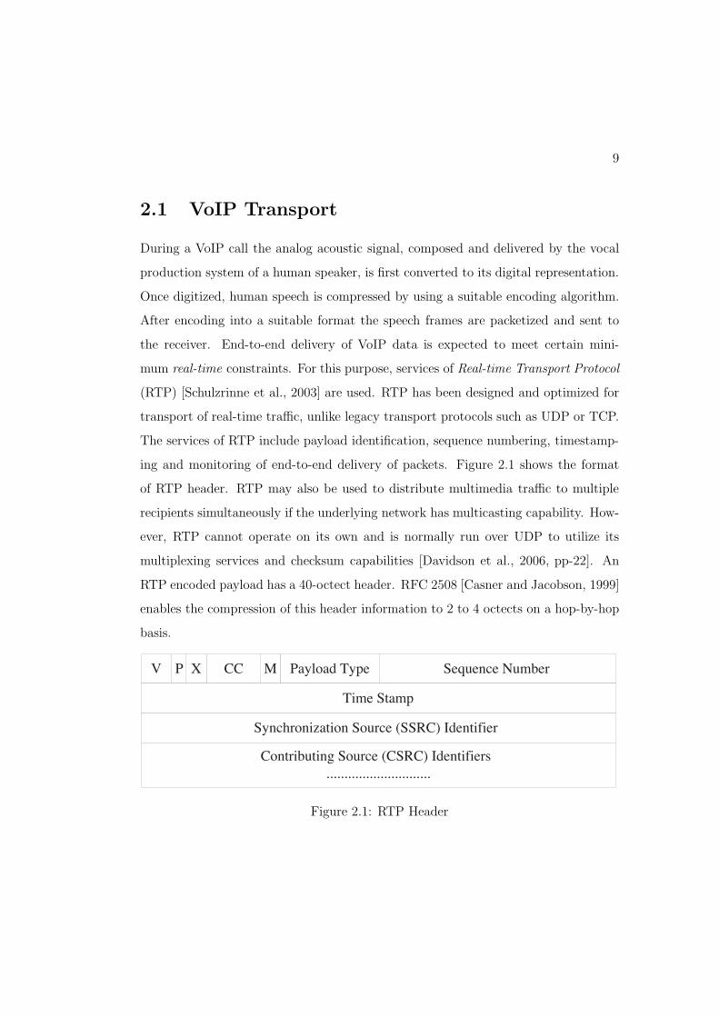
2.1 VoIP Transport

During a VoIP call the analog acoustic signal, composed and delivered by the vocal

production system of a human speaker, is first converted to its digital representation.

Once digitized, human speech is compressed by using a suitable encoding algorithm.

After encoding into a suitable format the speech frames are packetized and sent to

the receiver. End-to-end delivery of VoIP data is expected to meet certain mini-

mum real-time constraints. For this purpose, services of Real-time Transport Protocol

(RTP) [Schulzrinne et al., 2003] are used. RTP has been designed and optimized for

transport of real-time tra"c, unlike legacy transport protocols such as UDP or TCP.

The services of RTP include payload identification, sequence numbering, timestamp-

ing and monitoring of end-to-end delivery of packets. Figure 2.1 shows the format

of RTP header. RTP may also be used to distribute multimedia tra"c to multiple

recipients simultaneously if the underlying network has multicasting capability. How-

ever, RTP cannot operate on its own and is normally run over UDP to utilize its

multiplexing services and checksum capabilities [Davidson et al., 2006, pp-22]. An

RTP encoded payload has a 40-octect header. RFC 2508 [Casner and Jacobson, 1999]

enables the compression of this header information to 2 to 4 octects on a hop-by-hop

basis.

V P X CC M Payload Type Sequence Number

Time Stamp

Synchronization Source (SSRC) Identifier

Contributing Source (CSRC) Identifiers .............................

Figure 2.1: RTP Header

10

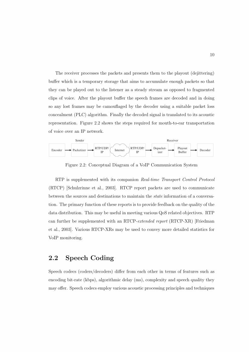
The receiver processes the packets and presents them to the playout (dejittering)

bu!er which is a temporary storage that aims to accumulate enough packets so that

they can be played out to the listener as a steady stream as opposed to fragmented

clips of voice. After the playout bu!er the speech frames are decoded and in doing

so any lost frames may be camouflaged by the decoder using a suitable packet loss

concealment (PLC) algorithm. Finally the decoded signal is translated to its acoustic

representation. Figure 2.2 shows the steps required for mouth-to-ear transportation

of voice over an IP network.

Encoder Playout Buffer

Depacket- izer

RTP/UDP/ IP

RTP/UDP/ IP Packetizer Internet Decoder

Sender Receiver

Figure 2.2: Conceptual Diagram of a VoIP Communication System

RTP is supplemented with its companion Real-time Transport Control Protocol

(RTCP) [Schulzrinne et al., 2003]. RTCP report packets are used to communicate

between the sources and destinations to maintain the state information of a conversa-

tion. The primary function of these reports is to provide feedback on the quality of the

data distribution. This may be useful in meeting various QoS related objectives. RTP

can further be supplemented with an RTCP-extended report (RTCP-XR) [Friedman

et al., 2003]. Various RTCP-XRs may be used to convey more detailed statistics for

VoIP monitoring.

2.2 Speech Coding

Speech codecs (coders/decoders) di!er from each other in terms of features such as

encoding bit-rate (kbps), algorithmic delay (ms), complexity and speech quality they

may o!er. Speech codecs employ various acoustic processing principles and techniques

11

to meet the listeners’ expectation of perceived speech quality. In terms of encoding

principles, speech codecs may be divided into two main categories; waveform and

parametric. Each one of these is discussed briefly in the following sections.

2.2.1 Waveform Codecs

Waveform coding methods relate to the time domain representation of the speech

signal. ITU-T G.711 [ITU-T, 1988b] is a primitive codec in this category. It gives

a transmission bit-rate of 64 kbps with a sampling rate of 8 kHz. It has two modes

of operation; A-law is used in Europe and µ-law is used in United States and Japan.

Waveform codecs also employ di!erential coding principles, where a given coded sam-

ple produced by the coder is a function of the current input sample of the speech signal

and the past n output samples of the coder. Transmitting the di!erence signal saves

bandwidth, as the average di!erence between the samples is smaller than their actual

amplitudes. Some examples of the di!erential coders include ITU-T G.726 [ITU-T,

1990a] and G.727 [ITU-T, 1990b].

2.2.2 Parametric Codecs

As opposed to waveform codecs, parametric codecs model the human vocal production

system, and attempt to extract a reduced set of parameters relevant to the speech

signal to be coded [Chu, 2003]. In doing so parametric codecs attempt to produce

codes of minimum data rate by exploiting the resonant characteristics of the human

vocal tract. The slow rate of change of signals originating in the vocal tract justifies

this approach. Thus, a small set of parameters is used to approximate the signal in

approximately a 30 ms wide window, during which the signal may be assumed to be

stationary. These parameters include the following:

• Up to a dozen coe"cients that define the resonant frequencies of the vocal tract.

12

• A binary indicator describing whether the excitation source (vocal cords) is

voiced or unvoiced.

• A value for the excitation energy.

• In case of a voiced signal, a value for pitch is also included.

Together, these parameters constitute a data frame. The state of the speech

waveform is approximated in this way by analyzing the speech waveform every 10

to 30 ms. Parametric codecs typically use linear predictive coding (LPC) [Makhoul,

1975] for optimization and computation of these parameters.

At the receiving side a corresponding decoder performs a synthesis operation on

these parameters to reproduce the original waveform. Data rates of parametric codecs

vary between 1.2 to 8 kbps for NB codecs. The rate depends on various factors that

include frame rate, the number of parameters in the frame and the accuracy with

which each parameter is coded.

Some examples from this family of codecs include ITU-T G.729 [ITU-T, 1996a],

ITU-T G.723.1 [ITU-T, 1996b], Adaptive Multirate Coding (AMR) [ETSI, 2000].

These codecs have also been utilized in this research.

2.2.3 Wideband Codecs

Speech codecs may also be categorized in terms of their audio transmission bandwidth

i.e. narrowband (NB) or wideband (WB). All the codecs listed in the previous section

belong to the NB type. In NB the audio transmission bandwidth is restricted between

200-3400 kHz typically. In WB this is increased to 100-7000 kHz. It is believed that

WB codecs may enhance speech quality as they make the speech sound more natural

to human ears. Examples include ITU-T G.722 [ITU-T, 1988a], G.722.1 [ITU-T,

2005b], G.722.2 [ITU-T, 2003d] and G.729.1 [ITU-T, 2006a].

13

2.2.4 Auxiliary Components

Apart from mere encoding and decoding of the speech, sophisticated codecs of the

present day are also equipped with auxiliary components that aim to enhance the

perceptual quality of speech. For instance, in order to regulate the input and the gain

of the output signal a codec may be equipped with an automatic gain controller (AGC)

[Chu, 2003, pp-319]. Similarly, background noise degrades the quality of the speech

signal. In order to alleviate this issue, a noise suppression or speech enhancement

algorithm may be applied to the speech signal [Diethorn, 1997]. Other significant

elements are silence suppression, dejittering bu!er and packet loss concealment. These

are discussed separately in the following sections.

2.2.4.1 Silence Suppression

Silence suppression, or discontinuous transmission (DTX), may also be implemented

in codecs whereby the periods of a conversation when a speaker is silent are not

coded and consequently not transmitted. DTX is aimed at bandwidth saving. A

voice activity detector (VAD) is used to implement DTX. A comfort noise signal may

instead be inserted in to the VoIP stream during the silent intervals [Zopf, 2002].

The processing of the speech stream by the VAD algorithm may lead to a clearly

audible distortion. This is attributed to the front-end clipping of the speech seg-

ments immediately following a silence interval, leading possibly to loss of informa-

tion [Davidson et al., 2006, pp-157].

2.2.4.2 Dejittering Bu!ers

An IP network introduces a variation in delay (jitter) on packets. Network jitter

is a result of queuing delay caused by the intermediate processing nodes (routers

and switches) of an IP network. As a consequence the decoder on the receiving end

14

may not receive a steady stream of speech frames. In order to provide the listener

with a continuous stream of speech, a VoIP application implements a dejittering

bu!er [Davidson et al., 2006, pp148-149]. A dejittering bu!er conceals the network

induced jitter by storing enough voice frames before presenting them to the decoder

to allow them to be fed at a constant rate into the decoder. Packets that arrive before

playout time are used to reconstruct a source signal. Packets that arrive after playout

time are discarded as they are of no avail in reconstructing an uninterrupted signal. A

secondary, but equally important, objective of a dejittering bu!er is to reduce packet

discards due to out-of-order arrivals. Thus, any such packets are reordered if they

arrive before their playout times have elapsed.

Bu!ering of packets increases the end-to-end delay of a VoIP stream. If delay is

large the user may loose interactivity with other participant(s) of the conversation.

This adversely a!ects the conversational quality of speech, hence imposing a limit

on the capacity of the dejittering bu!er. Various adaptive dejittering bu!ering ap-

proaches have been proposed either to achieve a minimum end-to-end delay given a

certain packet loss rate [Ramjee et al., 1994] [Moon et al., 1998] [Rosenberg et al.,

2000] [Fujimoto et al., 2002] or to achieve a minimum rate of packet loss due to late

arrivals [Ramjee et al., 1994]. However, this approach has recently been shown to

be inappropriate as it does not correlate well to the perception of speech quality in

a conversational sense [Sun and Ifeachor, 2006]. Lately there has been a growing

interest in designing adaptive dejittering bu!ers that dynamically adjust to a suit-

able combination of values for end-to-end delay and loss rate in pursuit of delivering

optimum speech quality, or conversely for achieving a minimum possible degradation

in quality [Sun and Ifeachor, 2006].

15

2.2.4.3 Packet Loss Concealment

For numerous reasons, a certain proportion of VoIP packets inevitably get lost during

transmission. To circumvent the adverse e!ects of packet loss on perceived quality,

speech codecs are typically equipped with a suitable Packet Loss Concealment (PLC)

algorithm.

PLC techniques may be sender based or receiver-based. In sender based PLC,

the sending device transmits additional information regarding the contents of speech

frames. In case of a packet loss this additional information is used to recover the

contents of the lost packet. Sender based PLC strategies include retransmission,

Forward Error Correction (FEC) [Rosenberg and Schulzrinne, 1999], frame interleav-

ing [Ramsey, 1970] and low bit-rate redundancy [Perkins et al., 1997]. In general

sender based techniques are not recommended to be used with interactive applica-

tions, such as VoIP, due to the imposed end-to-end delay [Perkins et al., 1998].

An alternative is to employ a suitable receiver based PLC technique. Such tech-

niques are useful for concealing packet losses containing voice data ranging between

4 to 40 ms and remain inferior to sender based schemes in terms of concealing the

losses. There are mainly three types of receiver based techniques:

• Insertion techniques: A packet is inserted in place of a lost packet. This could

be a silence packet or a noise packet or a repetition of a previous packet.

• Interpolation techniques: A suitable pattern matching technique or an inter-

polation method is used to search for a suitable waveform segment for a lost

packet based on the waveform of the neighboring (received) packet(s). Such

schemes are harder to implement but give better performance than insertion

based schemes. Waveform codecs like ITU-T G.711 [ITU-T, 1988b] use such

schemes.

• Regeneration techniques: In such a scheme the encoder’s state is restored by

16

relying on the parameters of the neighboring frame(s) of a lost one. Parametric

codecs normally implement such schemes.

A detailed survey on various PLC schemes has been given by Perkins et al. in [Perkins

et al., 1998].

2.3 VoIP Quality of Service (QoS)

ITU-T Recommendation E.800 [ITU-T, 1998d] defines QoS as follows:

“Quality of Service (QoS): The collective e"ect of service performance

which determines the degree of satisfaction of a user of the service.”

– ITU-T Recommendation E.800

To this aim, QoS provisioning is tantamount to collective optimization of the

performance of various network components so as to enhance the perceived quality

of VoIP. The traditional QoS mechanisms can be divided into two broad categories.

The first one is based on a class based prioritization of packets such as di!erentiated

services (DifServ) [Nichols et al., 1998]. DifServ uses the type of service (ToS) field of

the IP packet header to distinguish the packets into 4 priority classes. Based on this,

DifServ-enabled routers of an IP network take forwarding decisions in favor of the

packets with higher priority marks. Another approach is flow-based QoS provisioning

in which tra"c of a certain service may be associated with a particular network flow.

The flow is treated in the network according to its priority e.g., resource reservation

agreement. Examples of this include resource reservation protocol (RSVP) [Braden

et al., 1997] and multi protocol label switching (MPLS) [Rosen et al., 2001].

A recent approach is based on application level control of the transmission of VoIP

calls. In this a VoIP application adapts its configuration according to the operating

17

state of the network. Recently a perception based notion of QoS assessment has also

been adopted. According to this quality of speech, as perceived by the user of a VoIP

call, reflects upon the QoS level of the network. Feedback from the users’ experience

of VoIP is used to address the issues relevant to end-to-end delay, jitter and packet

loss. Operating conditions of the VoIP application such as codec bit-rate, or capacity

of dejittering bu!er are adapted to provide best possible quality to the user. Examples

of this include [Sun and Ifeachor, 2006] [Narbutt and Davis, 2005] [Hoene et al., 2005].

Apart from successful network operation and support for VoIP, issues related to

network security also fall under the umbrella of QoS provisioning. These may include

unauthorized monitoring, eavesdropping, misuse, human error and natural disaster

etc. QoS shall not be discussed further since it is beyond the scope of this dissertation.

2.4 Speech Quality Impairments

This section describes the various kinds and sources of impairments that may lead to

a degradation of speech quality of VoIP. Special emphasis is laid on those impairments

that deteriorate the quality of speech in a listening only scenario, albeit other scenarios

exist.

2.4.1 Packet Loss

A cardinal metric that a!ects VoIP quality is network packet loss. VoIP undergoes

packet loss due to the nature of the underlying packet switching network. It may

occur due to reasons such as link failures, network congestion, irredeemable errors

in packets and jitter bu!er packet overflow. An additional reason can be excessive

delay that is incommensurate with the play-out deadline of a packet or a frame. In

wireless networks packet loss may also occur due to ambient interference on the radio

18

link that may result in bit errors. The issue of bit errors and their e!ect on packet

loss is discussed in more detail in section 2.4.3. The degree of impairment associated

with packet loss may be characterized with the distribution of packet loss, packet size

and the type of method applied for packet loss recovery. Packet loss distribution is

discussed in more detail below.

2.4.1.1 Packet Loss Distribution

In the literature [Raake, 2006], the behavior of packet loss has been modeled using

a number of statistical distributions depending on the packet loss pattern. A given

packet loss pattern may in turn depend on the nature and operating conditions of

the underlying network. Packet loss is commonly assumed to follow a Bernoulli-

like distribution. This is also referred to as a random distribution in the literature

[Raake, 2006, pp-63]. Packet loss may exhibit temporal dependency too [Jiang and

Schulzrinne, 2000]. This implies that the loss of a single VoIP packet may lead to the

loss of immediately succeeding packets. This phenomenon leads to burstiness in the

behavior of packet loss.

More formally, burstiness implies that the loss of a certain packet depends on the

loss or reception of previous packet(s). A two state Markov chain has been proposed

by several authors to capture this temporal dependency e.g. [Bolot, 1993], [Sanneck

and Carle, 2000]. Each state of such a Markov model is used to depict a loss and a

no-loss scenario respectively. Figure 2.3 shows this model, where p is the conditional

probability of losing the packet numbered n+1 given that the nth packet is successfully

received. Similarly, q is the conditional probability of receiving the packet numbered

n + 1 given that the nth packet was lost. 1 ! q corresponds to the conditional loss

probability (clp). This model reduces to a Bernoulli model if p = 1 ! q. Usually

p < 1 ! q. This means that the probability of losing a packet numbered n + 1 is

higher when the nth packet is already lost as compared to the case when the nth packet

19

is successfully received. This condition models the bursty behavior in a meaningful

sense. Equation (2.4.1) corresponds to the mean loss rate (mlr) and is also known as

the unconditional loss probability (ulp).

mlr = ulp =p

p + q(2.4.1)

1 (NO LOSS)

0 (LOSS)

p 1-q

q

1-p

Figure 2.3: The 2-state Markov chain for modeling bursty packet losses

The burst and gap lengths (loss and no-loss runs) are geometrically distributed

random variables. mbl and mgl in (2.4.2) correspond to the means of the geometrically

distributed burst and gap lengths respectively [Sanneck and Carle, 2000] [Zwillinger,

2003].

mbl = 1/q, mgl = 1/p (2.4.2)

The values of p and q can be calculated from a network trace using gap and burst

length distribution statistics according to [Jiang and Schulzrinne, 2000], [Sanneck and

Carle, 2000]. The number of gaps having lengths i (i = 1, 2, ..., n ! 1) is denoted by

gi, where n! 1 is the length of the longest gap received. In a similar way the number

of bursts having lengths i (i = 1, 2, ..., m ! 1) is denoted by bi, where m ! 1 is the

length of the longest burst. Using the values of gi and bi the values of p and q can be

20

calculated in accord with (2.4.3) and (2.4.4).

p = 1 !

!

n!1"

i=2

gi. (i ! 1)

#

/

!

n!1"

i=1

gi.i

#

(2.4.3)

q = 1 !

!

m!1"

i=2

bi. (i ! 1)

#

/

!

m!1"

i=1

bi.i

#

(2.4.4)

Extended versions of the 2-state model are the Gilbert model 1 and the Gilbert-

Elliot model.

In order to accurately model the packet loss of up to n consecutively lost packets,

n-state models have been proposed separately by Sanneck and Carle [Sanneck and

Carle, 2000] and Yajnik et al. [Yajnik et al., 1999]. Such approaches are considered

favorable for capturing long term dependencies of packet loss. However, the modeling

process may become formidable for large n. In [Clark, 2001] Clark proposed a sim-

plified approach based on a 4-state Markov model still capable for capturing longer

term loss dependencies.

2.4.2 End-to-end Delay

End-to-end delay a!ects the interactivity of a VoIP conversation. It is composed of

various components such as processing delay by the codec, transportation delay that

may be incurred by the underlying IP network, delay induced by the dejittering bu!er,

and other signal processing components such as echo cancellers. Various components

of the network that may cause delay are listed in Table 2.1 along with the associated

values for delay.

ITU-T Recommendation G.114 [ITU-T, 2003c] provides guidance on the e!ect of

end-to-end one-way delay. According to this it is desirable to achieve an end-to-end

1The 2-state Markov model discussed above is frequently referred to as the Gilbert model inliterature, which is a misnomer.

21

Table 2.1: Various sources of delay with corresponding valuesDelay Source Typical Range (ms)Encoding 15–30IP Network 70–120Dejittering Bu!er 50–200Decoder 10–20Total 165–400

delay of less than 150 ms. However, regardless of the type of application, delay should

not exceed more than 400 ms.

As the focus of this thesis is on estimating listening quality of speech, end-to-end

delay and its e!ect shall not be discussed further in this thesis.

2.4.3 Bit Errors

Bit errors may occur in certain wireline and wireless communication technologies.

Wireless networks are more prone to bit-errors due to ambient interference on the

radio link. As VoIP is based on packet based communication, bit-errors are largely

taken care of by the UDP checksum. The checksum mechanism guards against any

violations in the UDP header as well as in the UDP payload by dropping packets with

incoherent checksums. Thus, flipping of even a single bit may have a considerable

e!ect on quality as it results in the loss of the whole VoIP packet. Consequently

this approach may lead to deterioration of quality as it does not allow for recovery

techniques to be applied to the speech frames. For instance, modern codecs, such as

GSM-FR and AMR-NB [ETSI, 2000], implement frame recovery mechanisms whereby

frame bits are classified according to their perceptual relevance, thus, allowing frames

to be dropped only when the most perceptually relevant bits are flipped during trans-

mission, and professing recovery otherwise. Implementation of this approach requires

one to disable the UDP checksums on the payload. In [Hammer et al., 2003] Hammer

et al. showed that by retaining and decoding VoIP frames with bit errors rates in the

22

range of 10!5–10!3 may result in a higher speech quality as compared to the scenario

when the erroneous speech frames are dropped.

2.4.4 Noise

A VoIP stream undergoes distortion due to noise from various sources. Firstly, noise

may be introduced due to codecs. Waveform codecs introduce signal-correlated noise

to the speech signal due to quantization. This noise is multiplicative in nature as it

is a function of the amplitude of the speech signal.

In the case that a codec implements a VAD algorithm, it may insert comfort noise

into the outgoing VoIP stream [Zopf, 2002]. Comfort noise may lead to a clearly

audible distortion as it is perceptually di!erent from the actual speech signal and the

background noise at the sending side [Raake, 2006, pp-84].

Ambient noise at both send and receive sides may also lead to considerable di"-

culties in conducting telephonic conversations. Background noise at the send side is

usually suppressed using a noise suppression or a speech enhancement algorithm.

2.4.5 Impairments due to Transcoding

Often participants of a call may not have similar codecs deployed on their telephony

equipment. An example of this is when one of the participants may be using VoIP with

ITU-T G.723.1 as the preferred codec, whereas the other participant may be using

PSTN, which uses ITU-T G.711. In this situation, in order to carry the speech of the

sending participant to the recipient, encoded speech would have to be converted to a

format amenable for processing by the codec implemented on the latter’s telephony

equipment. A similar phenomenon, termed as tandeming, is ubiquitous in wireless

networks for similar reasons, where the speech signal traverses a tandem of codecs on

its way to the intended recipient. Transcoding results in further degradation of the

23

speech quality compared to the cases where a single codec is used by both participants

of the call. It is reported by Campos Neto and Corcoran in [Neto et al., 1999] that

mean opinion score (MOS)2 may drop by more than 0.5 in the single tandem case

i.e., where speech is transcoded only once. Clearly, encoding and decoding the speech

signal multiple times has adverse e!ects on the quality of the output signal. A notable

e!ect of transcoding is that the quality degradation observed when the speech signal

traverses the network in one direction is not the same as if it were to traverse the

network in the opposite direction. This is to say that in a tandem of two codecs,

namely ‘X’ and ‘Y’, the quality degradation when the signal traverses the two codecs

in the order ‘X"Y’ is not the same as when it were to traverse them in the order

‘Y"X’. This asymmetry of distortions, as also reported in [Moller et al., 2006], is a

cause of numerous complications in speech quality estimation.

2.4.6 Miscellaneous Impairments

Various other important impairments or sources of impairments exist in a VoIP net-

work. Some of these are briefly described below.

Talker echo is a reflection of the talker’s own speech from a certain point in the

communication path. It occurs when the delay of the reflected speech signal exceeds

a certain threshold. In that case the reflected signal signal a!ects the interactivity of

the conversation. It is specifically important in situations where the network delay

may be considerable e.g. VoIP. Listener echo occurs as a result of multiple reflections

of a transmitted speech signal. The reflections may arise due to room acoustics at

the send side, or the user interfaces. Loudness and talker’s sidetone are other crucial

factors a!ecting quality perception. A detailed account of various impairments can

be found in [Raake, 2006].

2MOS terminology is explained in chapter 3

24

2.5 Conclusion

This chapter presented an introduction to VoIP, its various components, and the

associated factors that may a!ect speech quality. This thesis is focused on listening

quality of speech; the quality of speech in a listening only context. Delay related

impairments such as end-to-end delay and echo shall not be discussed further as they

a!ect the speech quality in a conversational scenario. The main impairments under

discussion would be those related to packet loss and speech codecs.

Chapter 3

Approaches to Speech QualityEstimation

3.1 Introduction

Speech quality estimation is vital to the evaluation of QoS o!ered by any telecommu-

nications network. Traditionally, speech quality is estimated using subjective tests. In

subjective tests, the quality of a speech signal under test is evaluated by a group of hu-

man listeners who assign an opinion score on an integral scale ranging between 1 (bad)

to 5 (excellent). The average of these scores, termed the Mean Opinion Score (MOS),

is considered as the ultimate determinant of the speech quality [ITU-T, 1996c]. Sub-

jective tests are, however, time consuming, expensive and hard to conduct. Moreover,

due to these reasons subjective tests are not easily repeatable; a feature that may be

desirable during transmission planning as well as network monitoring. To make up

for these limitations, there has been a growing interest in devising software based

objective assessment models. There are two kinds of objective assessment models,

namely, intrusive and non-intrusive. Intrusive models evaluate the quality of a dis-

torted speech signal in the presence of a corresponding reference signal. The current

25

26

ITU-T recommendation P.862 (PESQ) [ITU-T, 2001b] is an example of such an ap-

proach. Non-intrusive models, on the other hand, do not enjoy this privilege and base

their results solely on the estimated features of the signal under test. For this reason,

the results of the latter type of models are generally considered inferior to those of

the former.

Non-intrusive models can further be classified either as signal-based models or the

parametric ones. As the name suggests, signal-based models are based on the digital

signal processing of human speech. An example of such a model is the current,

state-of-the-art, ITU-T Recommendation P.563 for single-ended estimation of speech

quality [ITU-T, 2005d]. Parametric models, on the other hand, base their results on

various properties relevant to the telecommunications network. In the case of Voice

over IP (VoIP), these may be transport layer metrics such as packet loss, jitter and

end-to-end delay of a call. Such models are deemed suitable for real-time evaluation

of call quality. An example of a parametric model is the ITU-T G.107, commonly

referred to as the E-model [ITU-T, 2005a]. Figure 3.1 shows a classification of various

speech quality estimation methods.

Speech Quality Measurement

Subjective Methods Instrumental Methods

Listening-Only Conversational Intrusive Non-Intrusive

Signal-based Parametric

Figure 3.1: Various categories of speech quality assessment methods.

The rest of the Chapter is organized as follows. Section 3.2 discusses various

27

subjective methods for speech quality measurement. Section 3.3 discusses objective

methods for speech quality estimation.

3.2 Subjective Methods

The term subjective refers to the methods that employ human users to comment on

the quality of speech, without any aid or intervention of a computerized algorithm that

may itself have a role to play in the assessment of speech quality. This definition of

the term subjective has been considered as a misnomer according to Blauert [Blauert,

1997], as he states that quality opinions obtained through instrumental models are

also subjective. To support his argument he suggests that as a human subject is

behind the development of an instrumental model, the model imitates the human

developer. Moreover, since it is the human who ultimately interprets the results of

an instrumental model, the assessment procedure is subjective. In order to elucidate

the usage of the term subjective, Raake [Raake, 2006, pp-24] has made use of the

term auditory methods as the ones employing human subjects solely for assessment of

speech quality. Where quality is analyzed by employing a software or mathematical

model, the term instrumental is used as opposed to objective.

However, to keep in harmony with most of the literature on speech quality, the

methods employing only humans for the assessment of speech quality are referred to

as subjective methods in this dissertation. Any software based methods are referred

to as objective methods; these include both intrusive and non-intrusive methods.

In [Jekosch, 2005, pp-91] Jekosch has given the following definition of a speech

quality test:

“[a] routine procedure for examining one or more empirically restric-

tive quality features of perceived speech with the aim of making a quanti-

tative statement on these features.”

28

Based on this definition Raake categorizes subjective tests methods either as util-

itarian or analytical [Raake, 2006, pp-24]. According to this, a utilitarian method is

one that focuses on measurement of a single perceived feature or integral quality of

speech quality. An analytical method is one that investigates all or a subset of per-

ceived features associated with quality. In other words, utilitarian methods employ a

uni-dimensional quality rating scale. Analytical methods employ a multi-dimensional

analysis so as to reveal and quantify various perceived features of the speech signal

under test. In what follows, each of these methods is briefly described.

3.2.1 Utilitarian Methods

Utilitarian methods aim at a uni-dimensional analysis of the speech stimuli. Along

with this, e"ciency of test administration and data analysis and reliability of test

method are also primary goals. The main utilitarian tests are as follows:

3.2.1.1 Listening Only Tests

Most utilitarian methods are conducted as listening only tests (LOTs). Listening

tests vary from each other in terms of whether the test is conducted solely using the

speech signals to be tested or if the evaluators are also presented reference signals

corresponding to the various test stimuli. ITU-T Recommendation P.800 [ITU-T,

1996c] describes detailed procedures for conducting various types of listening tests.

Each of these is discussed below briefly.

Absolute Category Rating Tests

Absolute Category Rating (ACR) tests are most popular in telecommunications

for assessment of speech quality. ITU-T P.800 [ITU-T, 1996c] recommends various

scales depending on the focus of the test. The five point integral scale is most com-

monly used and it is referred to as the MOS scale. This is depicted in Table 3.1. In

29

these tests a group of subjects (testers) evaluate a speech sample composed of 2–5

short, independent and meaningful sentences, not exceeding 10 s, using the 5-point

scale. The opinions of each of these subjects are averaged to obtain the mean opinion

score (MOS).

Table 3.1: Five-point MOS scaleScore Interpretation

5 excellent4 good3 fair2 poor1 bad

Degradation and Comparison Category Rating Tests

Degradation category rating (DCR) or comparison category rating (CCR) tests em-

ploy a paired comparison of speech samples. In DCR, a testing subject is first pre-

sented with a clean speech signal. This is followed by assessment of the actual,

possibly degraded, speech signal. The subject is asked to rate the degradation of the

second sample with respect to the first.

In CCR the subject is presented with a pair of test stimuli. The second stimulus

is rated with reference to the first. Both stimuli are chosen randomly from a pool of

test stimuli.

By employing a comparison based approach, DCR and CCR methods give insight

into the speech quality with higher resolution. Both DCR and CCR also employ a

5-point category scale similar to the ACR tests. The details concerning these tests

are also listed in ITU-T P.800 [ITU-T, 1996c].

Isopreference Tests

This method is somewhat similar to the DCR or CCR tests. In this test a pair of

degraded and reference speech signals is presented to the listener for comparison.

The listening based comparison is continued by repeatedly changing the degradation

30

level of the reference signal until it yields the same quality as that of the degraded

signal. At this point, if a quantitative relation is known between the quality and the

degradation of the reference signal, it is used as an estimate of speech quality [Raake,

2006, pp-28]. ITU-T Recommendation P.800 [ITU-T, 1996c] defines the threshold

method which is closely related to this technique.

Continuous Evaluation

This method aims at addressing time varying degradations such as packet loss. It

is similar to the ACR method in the sense that evaluation takes place without any

reference signal. However, instead of a single quality estimate, the tester is asked

to continuously evaluate the speech signal over its whole duration with the help

of a slider; thus a continuous version of the 5-point rating scale of ACR method

is employed. After the continuous judgement the tester is also asked to estimate

the integral quality of the speech stimulus on ACR scale. This is used to make a

relationship with the instantaneous and integral estimates of quality.

During tests, the instantaneous quality estimates are made at least after every

half a second. The length of each stimulus may vary between 45–180 s. Both instan-

taneous ratings and integral quality estimates are averaged over subjects. This gives

a mean instantaneous rating profile and an integral MOS. ITU-T P.880 [ITU-T, 2004]

discusses continuous evaluation in more detail.

Third Party Listening Tests

These tests are listening tests but emulate conversation tests. A test subject is pre-

sented with a conversation between two speakers and is placed in the position of

one of them. Thus, the tester does not talk himself, but passively participates in

a conversational scenario. These tests are aimed at reducing the costs and e!orts

associated with data collection for conversational test scenarios at the expense of re-

alism of a conversational scenario. ITU-T Recommendations P.831 [ITU-T, 1998c]

and P.832 [ITU-T, 2000] discuss these tests in detail.

31

3.2.1.2 Talking and Listening Tests

These tests are closer to real conversational tests as opposed to the third party lis-

tening tests. In these tests the test subjects partake in conversation by listening and

talking. Due to the active role of the test subjects these tests have been used for

evaluation of echo cancelers [ITU-T, 1998c].

The realism of a conversation test is compromised due to the use of a Head and

Torso Simulator (HATS), that is employed as a conversation partner of the test sub-

ject. A HATS is composed of an artificial head with ears, equipped with microphones,

and an artificial mouth. The head is mounted on a dummy torso. The torso approx-

imates the sound shadowing introduced by a real person [Raake, 2006, pp-29-30].

3.2.1.3 Conversation Tests

Conversation Tests (CTs) employ human test subjects for the assessment of speech

quality. This method is superior to the other utilitarian methods due to this and

numerous other reasons. However, CTs have limited usability due to time and e!ort

required. Moreover, the tests cannot be repeated with the same degradation condi-

tions and conversational scenarios. ITU-T P.800 [ITU-T, 1996c] lays the procedure

for conducting CTs.

3.2.2 Analytical Methods

Speech quality is normally considered as a uni-dimensional entity. However, in certain

scenarios it becomes incumbent on transmission planners to analyze various aspects

of speech quality. Thus, a system engineer may be interested in finding out the

e!ect of a codec on naturalness as well as on smoothness of speech. This leads to a

requirement for multidimensional analysis of speech.

Analytical methods deal with identification and analysis of features that may a!ect

32

the perception of speech. This assumes that the perceived features have a correlation

with the perceived quality of the test stimuli. Analytical methods employ adroit sub-

jects who may distinguish between various features independent of their predilection

for a few. The very nature of these methods suggests that speech quality or perception

has multiple dimensions. Hence, these methods entail a multidimensional analysis.

Analytical methods shall not be discussed further in this thesis. Thorough discus-

sions on these methods can be found elsewhere in [Moller, 2000,Jekosch, 2005,Raake,

2006].

3.3 Objective Methods

Objective methods1 for speech quality estimation have become popular in recent

years. Objective methods aim at replacing human subjects with computational mod-

els for speech quality estimation. As a result, they provide a quick, cost e!ective

and easily repeatable way of measuring speech quality. Objective methods normally

output their results in the form of MOS. Thus, to di!erentiate between the results

obtained by objective and subjective methods ITU-T P.800.1 [ITU-T, 2003b] has rec-

ommended a mean opinion score terminology. According to this, the MOS obtained

by subjective tests are denoted by MOS-LQS (MOS-listening quality subjective) and

MOS obtained by objective tests are denoted by MOS-LQO (MOS-listening qual-

ity subjective). Objective methods can be subdivided into two categories; intrusive

methods and non-intrusive ones. In what follows both types of methods are discussed

briefly.

1Objective methods are also known as instrumental methods in literature.

33

3.3.1 Intrusive Methods

Intrusive models for speech quality estimation compare the speech signal under test

with a reference signal, which is normally a clean, distortion free version of the signal

under test. Intrusive models may be of two types depending upon the type of signal

processing employed for quality estimation. The first type of models, and the earliest

of all, employ time domain measures, such as signal to noise (SNR) ratio or segmental

signal to noise ratio (SNRseg) [Quackenbush et al., 1988]. Time domain models

are simple to implement and lend themselves easily to understanding by humans.

Such models are useful for estimating the performance of waveform codecs. However,

modern low bit-rate codecs employ complex human vocal production models and do

not render themselves to accurate analysis by time domain models. Such models are

also prone to time domain misalignments between the test and the reference signals;

slight misalignments may result in grossly erroneous estimates.

The second, and more sophisticated, type of models are based on perceptual do-

main measures of the human auditory system. So far such models have been most

successful in estimating speech quality and have gained the widest popularity. Such

models transform the time domain waveforms of test and reference speech signals into

a perceptually relevant domain.

Some examples of perceptual speech quality estimation include:

• PESQ (Perceptual Evaluation of Speech Quality) ITU-T Recommendation P.862

[ITU-T, 2001b].

• PSQM (Perceptual Speech Quality Measure) ITU-T Recommendation P.861

[ITU-T, 1998b].

• MNB (Measuring Normalizing Blocks) [Voran, 1999a] [Voran, 1999b]

34

3.3.1.1 The PESQ Algorithm

The PESQ algorithm is the current standard for speech quality estimation. It inherits

the psychoacoustic model of PSQM and the time alignment mechanism of Perceptual

Analysis Measurement System (PAMS) proposed by Rix and Hollier [Rix, 2000] and

Rix et al., [Rix et al., 2002]. The general structure of PESQ algorithm is given in

Figure 3.2. A textual description of the PESQ algorithm is as follows:

Perceptual Model

Internal Representation of

Degraded

Difference in Internal Representation Determines

the Audible Difference

Perceptual Model

Time Alignment

Internal Representation of

original

Cognitive Model

Reference Signal

Degraded Signal

Delay Estimates

Quality (MOS)

Figure 3.2: Intrusive speech quality estimation. Adapted from [ITU-T, 2001b]

1. Level alignment: Loudness levels of both distorted and reference signals are

adapted.

2. Input filtering: The speech signals are treated with a filter that emulates

the frequency response of the listening (receiving) end of a typical telephony handset.

Such a filter is specified as the (modified) IRS receive filter in ITU-T Recommendation

P.830 [ITU-T, 1996d].

3. Time alignment: The PESQ algorithm implements a complex time alignment

35

process. The time alignment computes time delay values and provides these to the

perceptual model to allow for a comparison of the corresponding parts of the original

and degraded speech signals. PESQ follows a multistage time alignment procedure

listed in [Rix et al., 2002].

4. Time-frequency transformation: The signals are transformed from time

domain to time-frequency domain using a short-time FFT. Signals are decomposed

into 32 ms frames with 50% overlap. Hann window is applied. A frame size of 32 ms

is chosen because this approximates the length of a typical phoneme. The start points

of frames of the degraded signal are shifted according to the time delay information

obtained from the time alignment module. The time axis of the original signal is kept

unmodified. If the delay increases, parts of the degraded signal are discarded. In case

if decrease in delay is observed, parts of the degraded signal are repeated.

5. Computation of pitch power densities: Frequency is converted from hertz

(Hz) to Bark scale [Zwicker, 1961]. The Bark scale is a nonlinear frequency scale

corresponding to the critical bands of hearing. A critical band refers to the frequency

bandwidth of a filter. It is believed that auditory signal is warped in the human ear

by a band of such filters, with center frequency spacings and bandwidths increasing

with frequency. The resolution decreases with increasing frequencies in a nonlinear

fashion. Thus, a Hz to Bark transformation is implemented by binning and summing

the per frame FFT bands according to a variant of the Bark scale transformation

followed by normalization of the sums. This results in pitch power densities of the

reference and degraded signals.

6. Calculation of the loudness densities: The pitch power densities of original

and degraded signals are transformed to a Sone loudness scale using Zwicker’s law

[ITU-T, 2001b]. The Sone loudness scale simulates the nonlinear relation between

the intensity of sound and its loudness perceived by humans.

7. Computation of the disturbance density: The signed di!erences between

36

the loudness densities of the distorted and reference signals are computed. A positive

di!erence, at any point, indicates the addition of other components, such as noise, to

the signal. Whereas a negative di!erence indicates that (spectral) components have

been omitted from the signal. These signed di!erences are stored in a 2-dimensional

array forming a raw disturbance density in the time-frequency plane. Additional

processing is applied to smooth the disturbance density. Specifically, masking by

loud spectral components in each time-frequency cell is modeled.

8. Modeling of the asymmetry e!ect: The PESQ algorithm models the asym-

metry e!ect [Beerends, 1995]. The asymmetry ensues from the fact that when a codec

distorts a speech signal, it will generally be di"cult to introduce a new component

in the time-frequency plane that will smoothly integrate with the speech signal. This

will result in a clearly audible distortion. If, on the other hand, a codec simply leaves

out a spectral component, the distortion will be less objectionable. The asymmetry

e!ect is modeled as a ratio between the distorted and the original pitch power den-

sities. The result of this step is a 2-D array containing an asymmetrical disturbance

density.

9. Aggregation of disturbance densities over frequency: The disturbance

densities calculated in the last two steps are integrated over frequency for each frame.

This results in two arrays of frame disturbances for corresponding densities.

10. Aggregation of disturbances over time: A two step aggregation of both

disturbances is performed at this stage. The first is a split second aggregation in which

disturbances corresponding to phonemes are aggregated for 20 successive frames. This

results in two disturbance arrays corresponding to syllables. This aggregation is per-

formed by employing L6 norm. Next the values of these disturbance arrays are ag-

gregated over the entire length of the speech signal using the L2 norm.

11. Computation of the PESQ score: The output of the PESQ algorithm

is a MOS score and it is a linear combination of the aggregated disturbance values

37

computed in the previous step. The linear combination was optimized for a large set

of subjective experiments. At the time of its standardization, the results of PESQ

algorithm had an average value of Pearson’s product moment correlation coe"cient

[Walpole et al., 1998] equal to 0.935 for a large number of subjectively evaluated

speech databases. Pearson’s product moment correlation coe"cient is normally used

to assay the prediction accuracy of an instrument model, with a value closer to 1

implying a better correlation of the model’s results with those of the subjective tests.

The PESQ algorithm outputs its results on the MOS scale and emulates ACR

tests. The PESQ algorithm was modified and extended numerous times. ITU-T

P.862.1 [ITU-T, 2003a] is currently the most up-to-date version. The PESQ algorithm

was initially designed for NB speech quality estimation. ITU-T P.862.2 [ITU-T, 2005f]

is a recent variant of the PESQ algorithm for speech quality estimation in a WB

context.

3.3.2 Non-Intrusive Methods

Non-intrusive speech quality estimation is a challenging problem in the sense that

a reference, or a clean, signal is not available to the computational model. Quality

estimates are based solely on the speech signal under test, or on the knowledge of the

system under test. Consequently, the results obtained by such models are also inferior

to those of intrusive models. However, they can be significant for live and real-time

evaluation of speech quality. These methods are also known as no-reference or single-

ended methods. Non-intrusive methods of speech quality estimation may further be

divided into two categories, namely parametric methods and signal-based methods.

Figure 3.3 gives a pictorial representation of such models. A brief description of these

methods is given in the following sections.

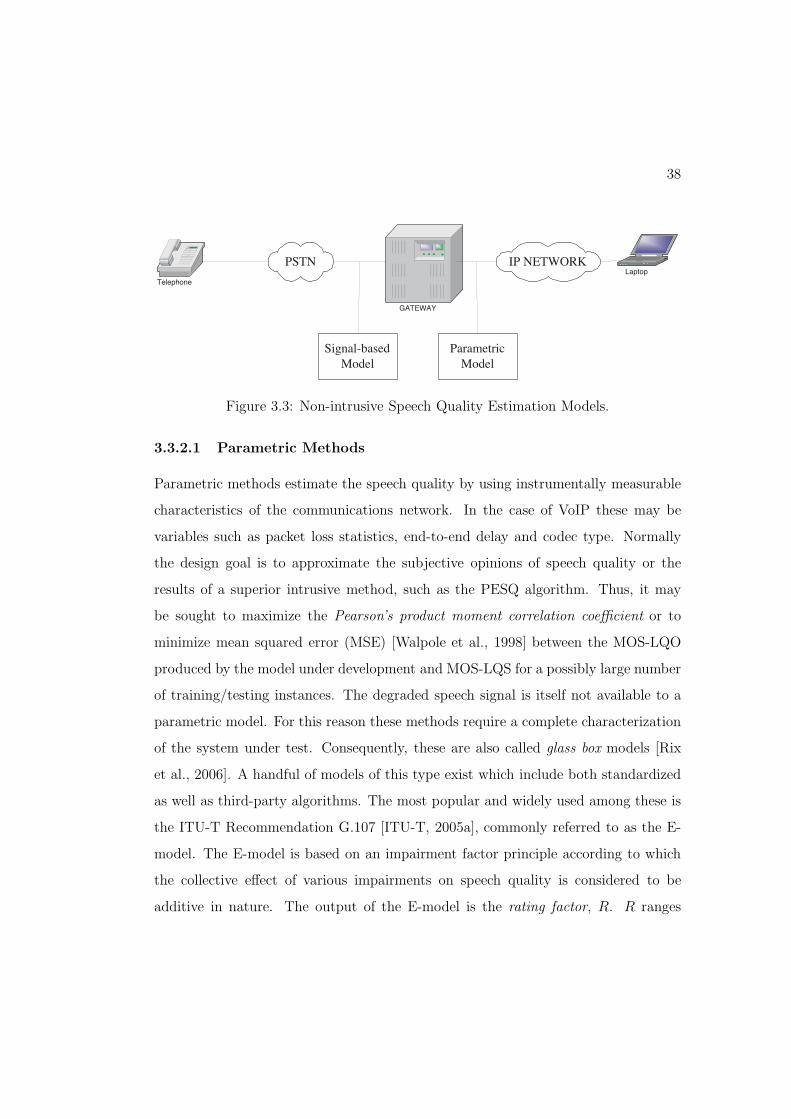
38

Laptop Telephone

GATEWAY

PSTN IP NETWORK

Signal-based Model

Parametric Model

Figure 3.3: Non-intrusive Speech Quality Estimation Models.

3.3.2.1 Parametric Methods

Parametric methods estimate the speech quality by using instrumentally measurable

characteristics of the communications network. In the case of VoIP these may be

variables such as packet loss statistics, end-to-end delay and codec type. Normally

the design goal is to approximate the subjective opinions of speech quality or the

results of a superior intrusive method, such as the PESQ algorithm. Thus, it may

be sought to maximize the Pearson’s product moment correlation coe!cient or to

minimize mean squared error (MSE) [Walpole et al., 1998] between the MOS-LQO

produced by the model under development and MOS-LQS for a possibly large number

of training/testing instances. The degraded speech signal is itself not available to a

parametric model. For this reason these methods require a complete characterization

of the system under test. Consequently, these are also called glass box models [Rix

et al., 2006]. A handful of models of this type exist which include both standardized

as well as third-party algorithms. The most popular and widely used among these is

the ITU-T Recommendation G.107 [ITU-T, 2005a], commonly referred to as the E-

model. The E-model is based on an impairment factor principle according to which

the collective e!ect of various impairments on speech quality is considered to be

additive in nature. The output of the E-model is the rating factor, R. R ranges

39

between 0 (poor quality) to 100 (optimum quality). An invertible relationship exists

between R and MOS. Three impairment factors are emphasized in the model. These

include, impairments that occur simultaneously with the speech signal, impairments

due to delay and impairments due to equipment such as packet loss and distortions due

to low bit-rate coding. ITU-T has devised a method to derive equipment impairment

factors for E-Model by using instrumental models such as PESQ [ITU-T, 2002]. E-

model was designed for transmission planning purposes initially. However, now it is

also being used in networks for on-line monitoring of speech quality [A. D. Clark,

1998]. E-model was originally developed for NB telephony. Currently its extension

for WB telephony is under progress [Moller et al., 2006].

A number of other third party algorithms also exist. Sun and Ifeachor [Sun and

Ifeachor, 2006] and Rosenbluth [Cole and Rosenbluth, 2001] have proposed logarith-

mic functions to compute impairment factors for the E-model. Sun and Ifeachor [Sun

and Ifeachor, 2006] used the PESQ algorithm as a reference to compute equipment

impairment functions.

In [Clark, 2001] Clark identified the recency e"ect. He stated that the impression

of an impairment on human memory fades as time passes. He emulated this innate

ability of humans to remember the e!ect of an impairment only for a certain amount

of time.

Sun and Ifeachor [Sun and Ifeachor, 2002a] and Mohamed et al. [Mohamed et al.,

2001,Mohamed et al., 2004] separately derived parametric models of speech quality

estimation in real-time using artificial neural networks (ANNs). Speech quality is

estimated in terms of MOS.

Hoene et al. [Hoene et al., 2004,Hoene et al., 2005] have employed a look-up table

based approach for the derivation of their quality model. In their scheme, the quality

estimates can also be used to dynamically adapt the playout time and codec’s bit-rate

to enhance perceived speech quality.

40

Conway [Conway, 2002,Conway, 2004] proposed an algorithm for estimating per-

ceptual quality of framed speech signals using the PESQ algorithm. In this scheme

the packet/frame loss pattern for a received packet/frame stream is computed. Lo-

cally, a clean speech signal is also maintained. The computed loss pattern is applied

to a copy of the locally stored speech signal. As a result a distorted speech signal is

formed with frame losses exactly in those locations as would be in the actual speech

stream delivered to the listener of the telephone call. The distorted speech signal

is compared with its clean version using the PESQ algorithm. The obtained result

reflects upon the users’ satisfaction of the call. A fundamental problem with this

approach is that it employs the PESQ algorithm whenever speech quality has to be

assessed, Whereas PESQ algorithm is both non real-time and compute intensive.

3.3.2.2 Signal-Based Methods

Signal-based non-intrusive models are preferable to parametric ones for various rea-

sons. Firstly, parametric models can be used only with certain types of networks, such

as VoIP. Secondly, signal-based models are more general in the sense that they are

applicable for a wider range of distortion conditions. Unlike the parametric models,

these models process the audio stream to extract the information relevant to distor-

tions in a signal. The estimated distortions are then converted into MOS-LQO for

that audio stream. Given this, a signal-based model may have two main modules. 1)

A feature extractor that processes the speech signal and extracts cogent distortion

indicators. 2) A mapping module that transforms the extracted features into MOS

estimates. The mapping part, also referred to as the cognitive part of the system,

may be derived by employing a suitable regression algorithm or a machine learning

technique. Signal-based methods are also referred to as black box methods as, either

no knowledge of the system under test is required or it is not available [Rix et al.,

2006].

41

Liang and Kubichek [Liang and Kubichek, 1994] proposed the first signal-based

model for speech quality estimation. In their work they used the perceptual linear

prediction (PLP) coe"cients [Hermansky, 1990] extracted from undistorted speech

signals. The PLP algorithm emulates the auditory processing of the human ear.

These coe"cients were used to train a code-book of reference centroids. PLP coe"-

cients of speech frames of a distorted speech signal were used to compute the Euclidean

distance from their nearest reference centroids. The time-averaged Euclidean distance

over the entire length of the speech signal was used as an indication of speech quality

degradation. This approach has been followed in numerous subsequent research stud-

ies. The model performance was assessed by using various distortion measures used

in vector quantization [Jin and Kubichek, 1995,Jin and Kubichek, 1996]. In [Picovici

and Mahdi, 2004] Picovici and Mahdi proposed to form a reference code-book of PLP

coe"cients of clean speech signals using the self organizing map [Kohonen, 1990].

In [Li and Kubichek, 2003] Li and Kubichek proposed a scheme based on a hidden

Markov model [Rabiner, 1989] to capture the temporal dependency between segments

of human speech. Recently Falk et al. [Falk and Chan, 2006] proposed a model in

which Gaussian mixture models [Everitt and Hand, 1981,Bishop, 1995] were trained

separately for PLP coe"cients of clean and distorted speech signals. These models

were used for computing consistency measures of the speech signal under test with

respect to clean and distorted reference mixture models. The consistency values were

mapped to MOS obtained by subjective tests using multivariate adaptive regressive

splines [Friedman, 1991].

In [Kim, 2004, Kim, 2005] Kim proposed an auditory model for non-intrusive

speech quality estimation (ANIQUE). The proposed model was based on temporal

envelope representation of the speech signal under test.

As opposed to modeling the human auditory system, Gray et al. proposed a

model based on human vocal production system [Gray et al., 2000]. It is based on

42

the premise that most distortions caused by the telecommunications systems cannot

be produced by human vocal production systems due to the limited motor mechanism

of the human vocal tract. Thus, the derived model was sensitive to the distortions

occurring in telecommunications networks.

3.3.3 ITU-T P.563

From 2002 to 2004 ITU-T held a competition to standardize a model for non-intrusive

speech quality estimation. Two models were submitted namely; ANIQUE and single-

ended assessment model (SEAM). The former was narrowly beaten by the latter.

SEAM was based on three di!erent models including the one proposed by Gray et

al. [Gray et al., 2000]. This was standardized as ITU-T P.563 [ITU-T, 2005d]. The

average correlation of MOS-LQO produced by ITU-T P.563 with MOS-LQS was 0.88

over the set of 24 subjective tests used for training and testing. The overall structure

of the P.563 algorithm is shown in Figure 3.4. It may be divided into three stages,

namely, preprocessing, feature, extraction and perceptual mapping. Each of these is

discussed below briefly.

1) Preprocessing: In this stage the signal is level normalized to -26 dBov2.

After this, two additional versions of the distorted signal are created. The first is

created by a filter having a frequency response similar to the modified intermediate

reference system (IRS) as described in ITU-T P.830 [ITU-T, 1996d]. IRS emulates

the frequency response of a standard telephony handset. The second version of the

normalized signal is created by using a fourth-order Butterworth high-pass filter with a

100-Hz cuto! frequency and a flat response for higher frequencies, thus emulating the

frequency response of cordless and mobile phones. Voice Activity Detection (VAD) is

also a part of the preprocessing stage that is used to discard speech sections shorter

2Decibels relative to the overload point of a digital system

43

Preprocessing

Pitch synchronous vocal tract model and LPC analysis

Ditortion specific parameters (noise, temporal clipping,

robotization)

Speech Reconstruction

and full reference perceptual model

Dominant distortion classification and perceptual weighting

Degraded Speech Signal

Figure 3.4: The structure of ITU-T P.563, adapted from [Rix et al., 2006]

than 12 ms and to join speech sections separated by less than 200 ms.

2) Feature extraction: This stage pertains to feature extraction which is applied

on the preprocessed versions of the signal. Feature extraction is based on three basic

principles. The first principle models the human vocal tract as a series of concatenated

tubes to reveal the anomalies in the speech signal as a function of abnormal variations

in the tubes’ sections. The statistics relevant to these anomalies form the speech

features.

The human vocal production system may be considered to have three components:

lungs as a source of air pressure, vocal chords as source of modulation and the vocal

tract as a resonating source. Thus, for voiced sounds, the air pressure created by

the lungs excites the vocal chords to create a low frequency, quasi periodic sound.

The spectral content of this sound is changed due to resonating characteristics of the

vocal tract. While speaking, the shape of the vocal tract is changed due to controlled

44

contractions and relaxations of its muscles. This changes the resonant frequencies of

the vocal tract, and consequently the spectral content of the speech. To this end,

Gray et al. attempted to capture the speech distortions, caused by communications

networks, by employing a human vocal production model [Gray et al., 2000]. The

vocal tract is modeled as a set of concatenated tubes with uniform, time-varying cross-

sectional areas. Here, it is assumed that most types of speech distortions cannot be

produced by a human vocal tract due to the limited and restrained movement of the

vocal tract muscles. In general terms, an implausible change in any of the tubes’ sizes

is considered as a distortion.

The second principle entails a reconstruction of a pseudo reference signal from the

signal under test to perform an intrusive quality evaluation of the speech signal to

estimate distortions. Signal reconstruction is done by performing a 10th order linear

predictive (LP) analysis of 5 ms frames of the distorted signal. LP coe"cients are

converted to line spectral frequencies followed by quantization to constrain them to

fit the vocal tract model of a typical human talker. LP is a popular speech analysis

technique used to represent characteristics of speech with a reduced set of parame-

ters [Gold and Morgan, 1999][pp280-291]. These quantized coe"cients are used to

reconstruct the pseudo reference signal. The di!erence between the pseudo reference

signal, in a spectral sense, and the signal under test gives a basic quality estimate

that is used as a feature for overall quality estimation.

The third principle is to features related to specific distortions encountered in voice

channels, such as temporal clipping, frame erasures, signal correlated and background

noise, robotization and speech level variation.

Perceptual mapping: According to the reference implementation of the algo-

rithm, a total of 43 features are extracted that depict various characteristics of the

speech signal under test. Based on a restricted set of key parameters, an assignment

to a dominant distortion class is made. A complete description of these features is

45

skipped here for brevity, but they can be divided into three distortion groups per-

taining to: 1) Unnaturalness of speech, 2) noise, and 3) interruptions, mutes and

temporal clipping. ITU-T P.563 uses a two step mapping process. First, an initial

quality estimate is made that is a linear combination of the values of a subset of

speech features that fall under a particular dominant distortion class. Second, a final

quality estimate is made that is again a linear combination of the initial quality esti-

mate and 11 additional features. P.563 has shown a high correlation with the human

evaluation of speech quality, ranging between 0.88–0.90 [ITU-T, 2005d] for various

ITU-T benchmark tests.

3.4 Conclusions

Various methods for speech quality estimation have been described in this chapter. It

has been discussed that subjective methods are the most reliable for obtaining speech

quality estimates. However, subjective methods are expensive and time consuming

to conduct. In order to circumvent these issues objective speech quality estimation

has become an active research area. The prediction accuracy of objective methods is

generally inferior to subjective methods. However, they are cost e!ective and compu-

tationally e"cient. The tests can also be repeated easily. The non-intrusive assess-

ment methods, as opposed to the intrusive methods, may also be used for continuous

and on-line monitoring of speech quality.

Chapter 4

Genetic Programming

4.1 Introduction

Genetic Programming (GP) [Koza, 1992] [Mitchell, 1997] is a biologically-inspired

machine learning technique. It seeks to generate plausible approximate solutions

to complex optimization problems by using concepts adopted, loosely, from natural

evolution. It has the advantage that, unlike many other optimization techniques, it

can generate solutions (or quasi-solutions) to problems in symbolic form. Although

the solution representation is problem specific, it is common to use mathematical

expressions or a subset of C/C++ for this purpose. GP produces human compre-

hensible results; an advantage when compared to approaches like Artificial Neural

Networks (ANNs) where making sense out of a trained network can be quite a chal-

lenge [Mitchell, 1997, pp-85]. Another crucial advantage is that GP is not merely

restricted to tuning the parameters of a pre-defined mathematical model like ANNs

and other numerical optimization techniques. Instead, as in this thesis, it also discov-

ers the model itself with the primary aim of optimizing a user defined error metric.

GP does not render numerical methods totally redundant, however. It has been used

46

47

to advantage in conjunction with numerical optimization techniques such as linear

regression [Keijzer, 2004], gradient descent [Topchy and Punch, 2001] and quasi-

Newton [Mugambi et al., 2004]. It has been suggested that the hybrid GP/numerical

methods yield superior results by allowing GP to focus at the truly innovative aspect

of the work, i.e., discovery of the model structure [Keijzer, 2004].

GP is coarsely modelled on natural evolution. Biological organisms aim to over-

come environmental obstacles and compete for resources in a bid for survival and

reproduction. GP evolves digital populations in a similar way. The environmental

challenges are defined by an error metric that each member of the population, an

individual or a candidate solution, seeks to minimise.

4.2 Execution Steps of Genetic Programming

Initially, the population is created by randomly generating a set of candidate solutions.

To allow this, the syntactic constituents of an individual are pre-specified in the

form of two sets: functions and terminals. Functions are exemplified by arithmetic

operators, trigonometric functions and boolean functions as they require operands

to produce an output. Terminals require no arguments. They may be, inter alia,

numeric constants, system variables and functions with constant inputs. An initial

population is generated by randomly picking from these sets, although other methods

exist [Banzhaf et al., 1998].

Each individual is tested on the given problem to assign it a measure of quality

which is called its fitness. The fitness of a GP individual determines the chances of

an individual surviving to the next generation or producing o!spring. The o!spring

result from introducing some variation into the selected parent(s). Normally, there

are two kinds of variation (or genetic) operators, crossover and mutation. Crossover

involves combining the genetic material of di!erent (normally two) individuals to

48

produce new solutions. Sometimes completely new genetic material is introduced into

the o!spring, albeit with a small probability. This phenomenon is called mutation,

and it is observed to be useful in GP by helping the system to work its way out of

local minima (which are undesired, but inevitable, artifacts of the objective function).

Clearly, the genetic operators of crossover and mutation must work in a manner

so that the resulting o!spring obey the syntactic constraints of the language used to

represent the solutions. To facilitate this, the GP-individuals are maintained with

data structures that are amenable to the carefully designed genetic operators. Ab-

stract syntax trees are by far the most popular choice, although linear structures are

also becoming common [Banzhaf et al., 1998] [O’Neill and Ryan, 2001]. Figure 4.1

shows two example GP individuals undergoing crossover and the resulting o!spring.

Note that the crossover point is selected randomly in each individual and the subtrees

rooted at those points are exchanged during the process. During mutation, a new

subtree may be randomly generated at the selected point, subject to a user specified

maximum depth limit. This is termed subtree mutation. Another type of mutation

is point mutation. In this type of mutation a point is randomly chosen in a given

individual and it is replaced by a new, randomly generated node. Figure 4.2 shows

examples of point and subtree mutation. As a result of the genetic operations the

resulting o!spring can be di!erent in size and shape from their parents as is the case

in the present example. This allows GP to explore a variable length solution space.

However, to stop the trees growing arbitrarily large, again a maximum depth limit

is employed. If the resulting o!spring have larger depths, they are discarded. As

stated earlier, the resulting o!spring should respect the syntactic constraints of the

underlying language. This implies, for instance, that in performing point mutation,

the randomly generated node should have the same arity as the node to be replaced.

Similarly, the subtrees chosen for crossover should have similar return data-types for

error-free execution of the resulting o!spring.

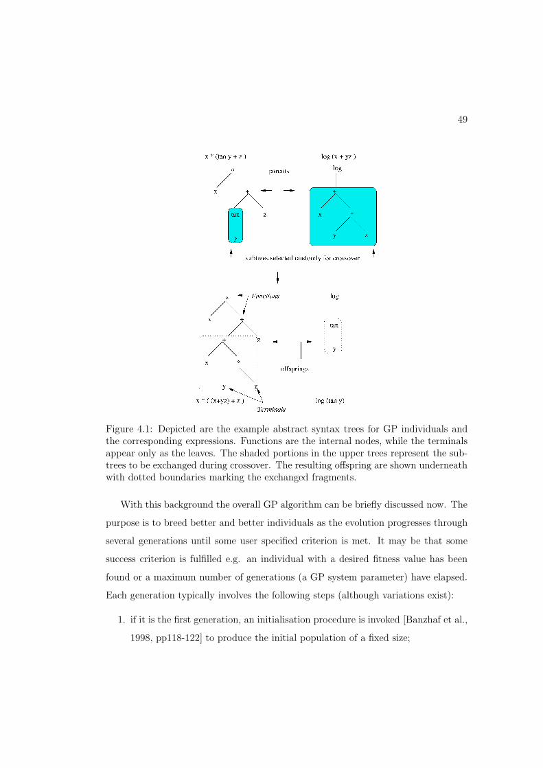
49

Figure 4.1: Depicted are the example abstract syntax trees for GP individuals andthe corresponding expressions. Functions are the internal nodes, while the terminalsappear only as the leaves. The shaded portions in the upper trees represent the sub-trees to be exchanged during crossover. The resulting o!spring are shown underneathwith dotted boundaries marking the exchanged fragments.

With this background the overall GP algorithm can be briefly discussed now. The

purpose is to breed better and better individuals as the evolution progresses through

several generations until some user specified criterion is met. It may be that some

success criterion is fulfilled e.g. an individual with a desired fitness value has been

found or a maximum number of generations (a GP system parameter) have elapsed.

Each generation typically involves the following steps (although variations exist):

1. if it is the first generation, an initialisation procedure is invoked [Banzhaf et al.,

1998, pp118-122] to produce the initial population of a fixed size;

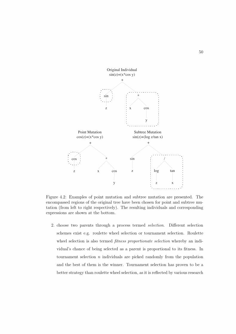
50

+

sin *

z x cos

y

Original Individual sin(z)+(x*cos y)

+

cos *

z x cos

y

+

sin /

z log tan

x z

Point Mutation cos(z)+(x*cos y)

Subtree Mutation sin(z)+(log z/tan x)

Figure 4.2: Examples of point mutation and subtree mutation are presented. Theencompassed regions of the original tree have been chosen for point and subtree mu-tation (from left to right respectively). The resulting individuals and correspondingexpressions are shown at the bottom.

2. choose two parents through a process termed selection. Di!erent selection

schemes exist e.g. roulette wheel selection or tournament selection. Roulette

wheel selection is also termed fitness proportionate selection whereby an indi-

vidual’s chance of being selected as a parent is proportional to its fitness. In

tournament selection n individuals are picked randomly from the population

and the best of them is the winner. Tournament selection has proven to be a

better strategy than roulette wheel selection, as it is reflected by various research

51

studies [Goldberg and Deb, 1990,Zhong et al., 2005];

3. crossover is applied to yield two o!spring which are then subjected to mutation.

Typically crossover is used with a high probability (e.g. 90%) while mutation

is used sparingly (1%);

4. evaluate the fitness of the two o!spring;

5. if the number of o!spring generated so far have reached a user specified limit,

follow on to the next step. Otherwise, go to step 2;

6. in this study, the o!spring and parent populations are considered together to

keep the best performers for the next generation. The rest of the individuals

from either pool are discarded. Other schemes may keep all the o!spring as the

population members for the next generation.

A number of generational cycles constitutes a GP run. Due to the stochastic

nature of the evolutionary process, each run of GP can produce individuals that are

di!erent from those of other runs despite the same system parameters and fitness

criteria. Therefore, it is a regular practice to conduct several runs in order to have

di!erent results of competitive quality and also to have a statistical justification of the

behavior of GP. Detailed accounts of various aspects of GP can be found in [Koza,

1992] [Banzhaf et al., 1998].

4.3 Numerical Parameter Tuning in GP

The essential merit of GP is its ability to find a viable structure of the target model.

In this, it di!ers from traditional optimization algorithms which aim at tuning the

parameters of an already specified model. Parameter tuning is also implicitly inherent

in GP’s search mechanism and may be accomplished in two di!erent ways. Firstly,

52

Koza has described this in [Koza, 1992], where he argues that GP can combine ter-

minals in an innovative fashion to find suitable coe"cients for evolving models. An

example is used to describe how (x/x) produces a constant value of 1, and eventually

applying the sin function to it produces a value of 0.841471.

However, this requires the application of possibly a large number of carefully

conducted crossover and/or mutation operations before the desired constant is found

and attached to an appropriate node of a GP in order to lend the desired e!ect.

This process may span a considerable number of generations and may in turn become

computationally ine"cient.

Secondly, when running a GP experiment that is expected to yield a final indi-

vidual with a few constants in it, it is common practice to attach the real number(s)

#, known as the ephemeral random constant, as terminal(s) to the individuals of the

first generation. This number is chosen probabilistically and, whenever it is chosen, it

is replaced with a randomly generated real number. Given that this number is chosen

probabilistically, an individual may have none or multiple random numbers attached

to it. These numbers either themselves, or in combination with other terminals and/or

functions, by forming more useful ones as mentioned above, serve as the constant co-

e"cients of the models being evolved. In fact, Koza noted in [Koza, 1992] that very

few of the initial constants appear unmodified in the final generation. In other words,

in most of the cases constants are combined with other terminals and functions to

form new ones. This is tantamount to the same problem stated above i.e. evolution

requires larger number of generations and leads to computational ine"ciency.

4.3.1 Hybrid Optimisation in GP

A few approaches have considered the problem of e"ciently attaching constants to

GP individuals. In [Keith and Martin, 1994] Keith and Martin employed a prefix

53

jumptable. In this approach, in order to accommodate constants a separate array of

floating point values is maintained. The genome simply consists of a linear array of

indices. In the case where a gene represents a constant, it points to an entry in the

array of floating point numbers. However, since the array is of a small size only a

small and finite set of constants can be used.

Additionally, various meta-heuristic and numerical parameter optimization meth-

ods have been used in conjunction with GP to create hybrid schemes for optimization.

In [Howard and D’Angelo, 1995] Howard and D’ Angelo proposed a hybrid GA-P al-

gorithm, where a genetic algorithm (GA) was used in conjunction with GP. Here

GP would evolve the structure of the individual programs and the constants of each

individual would be tuned with a GA. To achieve this, constants in a tree are indices

into an array of values. However, here each individual has its own array of values on

which search can be performed.

In [Sharman et al., 1995] Sharman et al. introduced a hybrid scheme by applying

simulated annealing to GP trees to evolve signal processing algorithms for a problem

concerning channel equalization. Here the mechanism of tuning constants is slightly

di!erent from that used in GA-P hybrid. In GA-P the constants are inherent parts of

the GP trees. Here the constants are associated as node gains to the edges between

nodes of a given GP tree. The methodology of appending node gains to edges is some-

what analogous to assigning weights to nodes in artificial neural networks [Mitchell,

1997]. The node gains associated with all the edges are maintained in a separate

array for each tree. The search is applied on this array for each tree. The simulated

annealing algorithm may be briefly described as follows:

Let !pq(i) be the node gain associated with edge pq at iteration i.

1. Perturb !pq(i) to get !"

pq(i) for all pq

2. Evaluate the fitness f "(i) using these perturbed parameters.

54

3. If (f "(i) > f(i)), then accept the perturbed node gains and continue.

4. Else, accept the perturbed node gains with some probability that is a function

of annealing temperature (T) and continue.

5. Reduce the annealing temperature (T) according to some cooling rate and go

to step 1. Stop if some user specified criteria is met.

The notions of annealing temperature and cooling rate are of central importance to

simulated annealing. During initial iterations the annealing temperature is kept high.

This allows the algorithm to accept perturbations that yield poor fitness with a higher

probability. This in turn allows the algorithm to, possibly, escape the trajectories

that lead to locally optimum solutions. As the simulation proceeds, the annealing

temperature is reduced at a certain cooling rate so as to adopt a more conservative

approach towards accepting bad perturbations. This allows the algorithm to converge

to some optimum solution in the vicinity [Kirkpatrick et al., 1983].

In [Esparcia-Alcazar and Sharman, 1997] Esparcia-Alcazar and Sharman further

expand and elaborate on their suggested methodology. They performed four evolu-

tionary experiments. In the first three they initialize node gains at random while

creating the initial population. In the fourth they do not use node gains while evolv-

ing models. In one of the first three experiments they induce Darwinian evolution

while adapting node gains with simulated annealing. Darwinian evolution implies

that the node gains learnt by an individual during its lifetime (i.e. learnt by simu-

lated annealing after its creation through crossover and mutation) are not carried over

to its o!spring. In another experiment Lamarckian evolution was emulated. Lamar-

ckian is another classical theory of evolution. It suggests that the behavior learnt by

an organism during its lifetime may be incorporated in to its genetic makeup, and

eventually may transmit to the o!spring. In this experiment the node gains learnt

by simulated annealing are carried over to the o!spring of that individual. Finally, in

55

the third experiment the node gains undergo some random mutations and are carried

over to the o!spring. Based on the results obtained for various problems they con-

clude that evolution along with parameter optimization (with simulated annealing)

performs better than with GP alone.

In [Topchy and Punch, 2001] Topchy and Punch performed non-linear optimiza-

tion using the gradient descent algorithm for the local search of leaf coe"cients of

GP trees. Moreover, the quasi-Newton method has been used to achieve the same

objective in [Mugambi et al., 2004].

There is a general consensus among researchers that for various problems hybrid

GP approaches perform better than GP alone. However, there are a number of issues

associated with using a parameter optimization algorithm along with GP to find ap-

propriate constants. The most predominant of these are the additional computational

requirements and the lack of knowledge of the particular problem domain.

Cogent questions which may arise while embarking on the implementation of a

hybrid optimization approach are: that how many coe"cients should the expected

model have, or what should be the range of those coe"cients? The answers to these

are usually not known for numerous problem domains and all an experimenter can do

is to rely on heuristics and guesswork. Similar questions as regards the configuration of

the optimization algorithm also need to be addressed. These include, for instance, in

the case where a GA is being used, questions regarding the population size, operator

probabilities, and number of generations. In simulated annealing these could be

number of iterations of the algorithm, annealing temperature and cooling rate. In

numerical optimization algorithms also, questions regarding the number of iterations

and learning rate are important. Clearly, some of these variables are clearly linked to

the nature of the underlying model and the number of coe"cients. However, due to

the varying nature of models at any given time in a GP population, these questions

cannot be addressed fairly. Normally the only choice the experimenter has is to rely

56

on empirical studies. The choice of these parameters also a!ects the performance of

the GP system. Thus, it becomes important to decide whether to tune the coe"cients

of all models being evolved by GP or to choose a subset of them.

4.3.2 Scaled Symbolic Regression

Normally the objective in GP based symbolic regression is to reduce the mean squared

error (MSE) between the instances of the target data of a particular problem domain

and the corresponding output values produced by the individuals of a GP system.

An individual that has a small MSE against the target data is considered as a better

candidate solution. MSE is given by equation (4.3.1)

MSE(y, t) = 1/nn

"

i

(ti ! yi))2 (4.3.1)

where y is a GP evolved function of the input parameters in this case (a mathematical

expression), yi represents the output value produced by y for the input case i and ti

represents the corresponding target value.

In [Keijzer, 2003,Keijzer, 2004] Maarten Keijzer proposed a technique to reduce

the scaled mean squared error (MSEs) instead,

MSEs(y, t) = 1/nn

"

i

(ti ! (a + byi))2 (4.3.2)

where a and b adjust the slope and y-intercept of the evolved expression to minimise

the squared error. They are computed as follows:

a = t ! by, b =cov(t, y)

var(y)(4.3.3)

In e!ect this scheme linearly regresses a given model to the target data during evo-

lution. This scheme has some special properties. Firstly, it is expected to perform

better than the simple MSE measure for most of the problems in symbolic regres-

sion. Rather, it has been proven by Keijzer in [Keijzer, 2004] that MSEs $ MSE for

57

any arbitrary problem concerning symbolic regression. The introduction of the slope

and intercept term make it easier for the GP to learn constant terms through linear

regression, which would otherwise be di"cult to search.

Another crucial advantage of this scheme is that it is computationally cheaper than

most of the other hybrid approaches. The operations defined by equation (4.3.3) can

be performed in O(N) time [Keijzer, 2003].

4.4 Advantages of GP

GP searches for a plausible solution from the space of computer programs. The search

process begins with a set of randomly generated programs in the search space. These

programs correspond to points in the GP search space. The programs with possibly

better quality are used to generate new programs corresponding to new points in the

search space using genetic operators such as crossover, mutation, reproduction etc.

The process is repeated iteratively until an individual program is found that meets

the desired performance criterion.

The great benefit of GP lies with its ability to search for the appropriate structure

of a target solution. To this end, GP is distinguishable from traditional optimization

approaches. It has already been mentioned in section 4.3 that some capability for

finding appropriate constants for the target model is inherent in GP. Such a capability

can also be enforced by hybridizing GP with an appropriate parameter optimization

algorithm. Altogether GP is a useful tool for learning models of an arbitrary intricacy.

This may include linear as well as nonlinear models. GP also has an additional

advantage of pruning o! the redundant system information during evolution. Since

GP’s evolutionary process follows the ‘survival of the fittest’ paradigm, it is likely to

weed out individuals having redundant system variables as genomes. To the contrary,

only individuals that depend on the salient system variables potentially survive to the

58

end of a run. This can be useful in finding concise models that depend on the relevant

data. To this end, GP also has the ability to perform a principal components analysis

of a particular problem domain. Lastly, given that GP embodies a stochastic search

technique, it has the ability to find a globally optimum model for a given problem

domain.

4.5 GP environment

For most of the work GPLab was used as the preferred GP environment. GPLab1

is a Matlab toolbox for GP developed by Sara Silva. As compared with the GP

environments built in other programming evironments it has the benefits of being

easily configurable and easy to program. However, it is computationally much slower

than contemporary systems written in laguages such as C or Java.

For some experiments, concerning the development of a signal-based model, a new

GP environment was developed in Java. Its software design was inspired from Beagle

Puppy2 software [Gagne and Parizeau, 2006]. Beagle Puppy is a GP environment

written in C. Some features were inherited from GPLab and research literature on

other useful techniques. A capability of hybrid optimization was also introduced by

implementing and integrating a GA to it. The modular design of this system allows

for easy integration of any of the other parameter optimization techniques with it.

Salient features of this system are described in more detail in section 7.3.1.

1http://gplab.sourceforge.net/2http://beagle.gel.ulaval.ca/puppy/

Chapter 5

Real-Time, Non-IntrusiveEvaluation of VoIP

5.1 Introduction

In this chapter we employ a Genetic Programming (GP) based symbolic regression

approach to estimate VoIP speech quality as a function of impairments due to IP

network and encoding algorithms. It was suggested earlier (in chapter 4) that the

main advantage of GP is that it can produce human-readable results in the form

of analytical expressions. Moreover, GP deals with the significant input parameters

and aids in the automatic pruning of irrelevant ones. These features of GP make

our results superior to the past research based on Artificial Neural Networks (ANNs)

by Sun and Ifeachor [Sun and Ifeachor, 2002a], Mohamed et. al. [Mohamed et al.,

2001] [Mohamed et al., 2004] and on lookup tables by Hoene et. al. [Hoene et al.,

2004]. We have employed a number of modern narrowband (NB) codecs to derive

speech quality estimation models. We have also used the NB version of PESQ as

a reference for evolutionary modeling. The results of proposed models show a high

correlation with PESQ. Moreover, our models are suitable for real-time and non-

intrusive estimation of VoIP quality.

The rest of the chapter is organized as follows: Section 5.2 describes the VoIP

59

60

experiment environment to gather the relevant data characterizing the speech tra"c.

Section 5.3 elucidates how this data is used to evolve the speech quality estimation

models. Section 5.4 presents the results and carries out an analysis of the current

research. Section 5.5 performs a descriptive comparison of the research presented in

this chapter with existing approaches. The chapter concludes in section 5.6 outlining

the major achievements and future ambitions.

5.2 VoIP Tra"c Simulation

A simulation based approach was pursued for this research. Such an approach has

been employed by various authors such as [Pennock, 2002] [Sun and Ifeachor, 2002b].

The main advantage of this approach is that various network distortion scenarios

can be emulated precisely. Moreover, the tests are easily repeatable. This section

describes the VoIP experiment methodology employed in this work.

A schematic of the simulation environment is shown in Figure 5.1. The system

includes a speech database, encoder(s)/decoder(s), a packet loss simulator, a speech

quality estimation module (PESQ), a parameter extraction module for computing

the values of di!erent parameters and a GP based speech quality estimation model.

A VoIP packet may either have talkspurt frames or silence frames included in it.

Speech Database

Model Evolved By GP

Paremeter Extraction

Decoder Loss Simulator Encoder

Quality measure (PESQ)

Reference speech signal

MOS-LQO GP

Degraded speech

MOS-LQO PESQ

VoIP Traffic parameters

Figure 5.1: Simulation System for Speech Quality Estimation Model

These frames can be distinguished if Voice Activity Detection (VAD) is enabled at

61

the encoder. In this case a silence frame is represented by an SID (Silence Insertion

Description) frame. In the rest of the Chapter any network parameters subscripted

with V AD correspond to talkspurt frames only. Unsubscripted parameters corre-

spond to real network tra"c. For instance, any use of the term mlrV AD refers to

mean loss rate of talkspurt frames only. The term mlr, however, refers to the mean

loss rate of the overall network tra"c of a particular VoIP call.

Three popular NB codecs were chosen in the current research, namely; G.729 CS-

ACELP (8 kbps) [ITU-T, 1996a], AMR-NB [ETSI, 2000] and G.723.1 MP-MLQ/ACELP

(6.3/5.3 kbps) [ITU-T, 1996b]. All of these are based on Linear Predictive Coding

(LPC) of speech. LPC is a scheme whereby the spectral envelop of human speech can

be represented in a compressed form. AMR was used in its 7.4 and 12.2 kbps modes

whereas G.723.1 was used in its 6.3 kbps mode only. All of these low bit-rate codecs

aim at VoIP tra"c bandwidth saving. These codecs also have built-in VAD and PLC

mechanisms.

The choice of network simulation characteristics was driven by ITU-T Recom-

mendation G.1050 [ITU-T, 2005c] which describes a model for evaluating multimedia

transmission performance over an IP network. Bursty packet loss was simulated using

the 2-state Markov model described in section 2.4.1.1 (Figure 2.3). It also models

packets discarded by the playout bu!er due to late arrivals. Packet loss was simulated

for di!erent values of mlr and conditional loss probability (clp). Twelve di!erent val-

ues for mlr were chosen; 0, 2.5, 5, 7.5, 10, 12.5, 15, 20, 25, 30, 35 and 40%. The peak

loss-rate (i.e. 40%) was kept an order of magnitude higher than that specified for an

unmanaged network in ITU-T G.1050 (i.e. 20%) so as to gather more representative

data for model derivation. For each value of mlr, clp was set to 10, 50, 60, 70, and

80%.

After subjecting the VoIP streams under test to various network impairments,

they were evaluated using NB version of the PESQ algorithm. The PESQ algorithm

62

compares a degraded speech signal with a reference (clean) speech signal and com-

putes an objective MOS score ranging between -0.5 and 4.5, albeit for most cases

the output will be between 1.0 and 4.5. It must be mentioned that PESQ simulates

a listening test and is optimized to represent the average evaluation (MOS) of all

listeners. It is statistically proven that the best possible result that can be obtained

from a listening only test is never 5.0, hence it was set to 4.5 [ITU-T, 2001b]. The

PESQ algorithm is widely acclaimed for its high correlation with the results of formal

subjective tests for a wide range of network distortion conditions. It is the current

de jure standard for objective speech evaluation specified by ITU-T. In the current

context, the MOS scores obtained by the PESQ algorithm and the MOS predicted

by the GP based model are di!erentiated by the abbreviations MOS-LQOPESQ and

MOS-LQOGP respectively. The term MOS-LQO is an acronym for Mean Opinion

Score-Listening Quality Objective and the various subscripts are used to identify the

objective quality estimation models used. This terminology is based on [ITU-T,

2003b].

Altogether, five VoIP tra"c parameters have been chosen in the current analy-

sis which form the input variables for evolutionary modeling. These parameters are:

codec bit-rate (kbps), packetization interval (ms) (abbreviated as PI), frame duration

(ms), mlrV AD and mblV AD (mean burst length of talkspurt frames) . A lower value

of bit-rate corresponds to a higher compression of the speech signal, thus resulting in

a lower bandwidth requirement at the expense of quality. The packetization interval,

which is the payload size of a VoIP packet, was varied between 10 to 60 ms. Consid-

erable bandwidth saving can be achieved by encapsulating multiple speech frames in

one VoIP packet thus reducing the need for RTP/UDP/IP headers that would have

been required for encapsulation and transportation of speech frames if they were to

be sent individually. However, higher packetization intervals have certain associated

drawbacks too. First, the end-to-end delay of the VoIP stream is increased as the

63

sender has to bu!er speech frames for a considerable duration before subsequent

frames become available by the encoder. Second, for a large packetization interval,

typically higher than 40 ms, loss of a single packet results in noticeable degradation of

speech quality. Hence, packetization interval presents a trade-o! between the speech

quality and bandwidth saving. Frame duration has a similar e!ect on the quality as

that of packetization interval. Higher frame durations may have other disadvantages,

for instance, in LPC a speech signal is assumed to be stationary (non-transient) for a

given frame duration. However, for higher frame durations this assumption may con-

siderably deviate from the reality. Thus, a codec with such a feature may distort the

final speech content. The parameter extraction module (Figure 5.1) is used to obtain

the values of the aforementioned parameters from the VoIP tra"c stream under test.

The corresponding MOS-LQOPESQ of the decoded VoIP stream under test subjected

to these network conditions forms the target output value for training purposes. In

actual VoIP applications this information would be gathered by parsing the RTP

headers and bitstreams of the encoded frames. The information would then be used

as an input for the GP based model to estimate MOS-LQOGP after processing.

5.3 Experimental Setup

As discussed earlier GP was the machine learning algorithm of choice for deriving a

mapping between network tra"c parameters and VoIP quality. GPLab was used as

the preferred GP environment in this study. Four GP experiments with di!erent con-

figurations were conducted for empirical reasons. The common parameters of all the

experiments are listed in Table 5.1. In all of the experiments the population size was

set to 300. Each experiment was composed of 50 runs whereas each run spanned 50

generations. Adaptive genetic operator probabilities were used [Davis, 1989]. In this

scheme the operator probabilities are changed at run-time. The algorithm keeps track

64

of some information regarding each new o!spring that is produced. This includes the

operators used for its creation and identities of its parents. Moreover, information

on how much better (or worse) a given o!spring is when compared to the best or

worst individual of the preceding generation is also included. An o!spring is assigned

a credit based on this information. All of this information related to o!spring is

fed to a repository that can hold a fixed number of entries. The entries enter and

leave this repository on a first in first out basis. After every predefined interval, the

performance of each genetic operator is computed by summing the credits of all o!-

spring in the information repository, and dividing the sum by the number of o!spring

in the repository produced by the respective operator. A percentage of the current

value of each operator’s probability is changed by a value proportional to the value

of performance of the respective operator.

Tournament selection with lexicographic parsimony pressure (LPP) [Luke and

Panait, 2002] was used in all of the experiments. In this selection strategy a group

of G (G % 2) individuals is picked randomly from the current population. The

individual with the highest fitness in the group is selected as a parent. In the case

of a tie between two or more individuals, their expression sizes are compared with

the smaller individual winning out. If both fitness and size are the same then an

individual is chosen at random. This strategy prefers smaller individuals and helps in

reducing the tendency to produce over-complicated expressions and consequently code

growth. The phenomenon of growth is also referred to as code bloat in GP. Survival

was based on elitism. The elitist criterion was such that half of the population of a new

generation would be composed of best individuals from both parents and children.

The other half of the population would be formed of remaining children on the basis

of fitness. This elitism criteria is termed as half elitism in GPLab.

In experiment 1 mean squared error (MSE) was used as the fitness function and

tournament size was set to 2. For experiment 2 (and subsequent experiments) scaled

65

Table 5.1: Common GP Parameters among all experimentsParameter ValueInitial Population Size 300Initial Tree Depth 6Selection Lexicographic Parsimony Pressure TournamentTournament Size 2Genetic Operators Crossover and Subtree MutationOperators Probability Type AdaptiveInitial Operator probabilities 0.5 eachSurvival Half ElitismGeneration Gap 1Function Set plus, minus, multiply, divide,sin, cos, log2, log10,

loge, sqrt, power,Terminal Set Random real-valued numbers between 0.0 and 1.0.

Integers (2-10). mlrV AD, mblV AD, PI, br, fd

mean squared error (MSEs) was used as the fitness criterion and is given by equation

(5.3.1).

MSEs(y, t) = 1/nn

"

i

(ti ! (a + byi))2 (5.3.1)

where y is a function of the input parameters (a mathematical expression), yi repre-

sents the value produced by a GP individual and ti represents the target value which

is produced by the PESQ algorithm. a and b adjust the slope and y-intercept of the

evolved expression to minimize the squared error. This approach is known as linear

scaling [Keijzer, 2004] and was also discussed in section 4.3.

Experiment 1 employed protected versions of various functions as these are im-

plemented in GPLab like most of the contemporary GP systems. Thus, to protect

against division by zero, GPLab has a division function, divide, that returns a value

of 0 if the denominator is equal to 0. Similarly, the sqrt function also returns 0 upon

receiving a non-positive number as an input. As another example, the logarithmic

functions return 0 upon receiving 0 as input. These protections are aimed at prohibit-

ing these functions from returning undefined values and/or complex numbers, and to

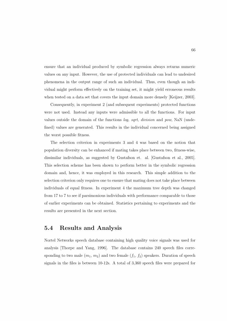
66

ensure that an individual produced by symbolic regression always returns numeric

values on any input. However, the use of protected individuals can lead to undesired

phenomena in the output range of such an individual. Thus, even though an indi-

vidual might perform e!ectively on the training set, it might yield erroneous results

when tested on a data set that covers the input domain more densely [Keijzer, 2003].

Consequently, in experiment 2 (and subsequent experiments) protected functions

were not used. Instead any inputs were admissible to all the functions. For input

values outside the domain of the functions log, sqrt, division and pow, NaN (unde-

fined) values are generated. This results in the individual concerned being assigned

the worst possible fitness.

The selection criterion in experiments 3 and 4 was based on the notion that

population diversity can be enhanced if mating takes place between two, fitness-wise,

dissimilar individuals, as suggested by Gustafson et. al. [Gustafson et al., 2005].

This selection scheme has been shown to perform better in the symbolic regression

domain and, hence, it was employed in this research. This simple addition to the

selection criterion only requires one to ensure that mating does not take place between

individuals of equal fitness. In experiment 4 the maximum tree depth was changed

from 17 to 7 to see if parsimonious individuals with performance comparable to those

of earlier experiments can be obtained. Statistics pertaining to experiments and the

results are presented in the next section.

5.4 Results and Analysis

Nortel Networks speech database containing high quality voice signals was used for

analysis [Thorpe and Yang, 1996]. The database contains 240 speech files corre-

sponding to two male (m1, m2) and two female (f1, f2) speakers. Duration of speech

signals in the files is between 10-12s. A total of 3,360 speech files were prepared for

67

various combinations of afore-mentioned values of network tra"c parameters. The

experiment parameters include frame duration, bit-rate, packetization interval, mlr

and clp. 70% and 30% of the data of distorted speech files corresponding to speakers

m1 and f1 were used for training and testing of the evolutionary models respectively.

Distorted speech files corresponding to speakers m2 and f2 were used to validate the

performance of the chosen model against speaker independent data. In other words,

network tra"c parameters and corresponding MOS-LQOPESQ of 1177, 503 and 1680

speech files were used for training, testing and validation respectively.

Table 5.2(a) lists the statistics about the MSE of the training/testing data and of

final tree size (in terms of number of nodes) of the 4 experiments under consideration.

A Mann-Whitney-Wilcoxon test was also performed to decide if a significant di!erence

exists between the experiments. Its results are tabulated in Table 5.2(b). At 5%

significance level a ’0’ in the tableau indicates that no significant di!erence exists

between the two experiments with respect to that metric (i.e. MSEtr, MSEte or

Size). A ’1’ indicates the converse and an ‘x’ marks that the metric is not to be

compared with itself.

Table 5.2: Statistical analysis of the GP experiments(a) MSE Statistics for Best Individuals of 50 Runs for experiments 1-4

Sim1 Sim2 Sim3 Sim4Stats MSEtr MSEte Size MSEtr MSEte Size MSEtr MSEte Size MSEtr MSEte SizeMean 0.0980 0.1083 42.6 0.0414 0.0430 38.8 0.0434 0.2788 28.5 0.0436 0.0436 18.0Std.Dev. 0.0409 0.0507 24.1 0.0040 0.0044 21.2 0.0042 1.0986 15.1 0.0037 0.0060 7.1Max. 0.2135 0.2656 103 0.0543 0.0568 104 0.0519 6.8911 74 0.0520 0.0782 38Min. 0.0449 0.0464 8 0.0368 0.0370 5 0.0378 0.0390 9 0.0370 0.0387 8

(b) Results of Mann-Whitney-Wilcoxon Significance Test

Sim1 Sim2 Sim3 Sim4Stats MSEtr MSEte Size MSEtr MSEte Size MSEtr MSEte Size MSEtr MSEte SizeSim1 x x x 1 1 0 1 1 1 1 1 1Sim2 1 1 0 x x x 1 0 1 1 1 1Sim3 1 1 1 1 0 1 x x x 0 0 1Sim4 1 1 1 1 1 1 0 0 1 x x x

68

A keen look at the tables 5.2(a) and 5.2(b) shows that experiment 2 (which used

linear scaling) performed significantly better than experiment 1. When we compare it

with experiment 3, we see that experiment 3 produces significantly smaller trees than

experiment 2, albeit with marginally inferior fitness. Finally, experiment 4 exhibits

similar traits, as its fitness is marginally worse again, although its trees are signifi-

cantly smaller. The objective in the current research was to find fitter individuals

with small sizes. Hence, experiment 4 was scavenged for plausible solutions.

Figure 5.2 delineates the significance of various network tra"c parameters in terms

of the number of best individuals using them in each of the four GP experiments.

It turns out that mlrV AD had a 100% utility in all of the experiments. Codec bit-

rate (br) and frame duration (fd) were the second and third most frequently availed

parameters respectively. Where as, both PI and mblV AD have shown advantage in

least number of runs of all experiments.

Sim1 Sim2 Sim3 Sim40

50

100fdbrPImlrVADmblVAD

Figure 5.2: Percentage of the best individuals employing various input parameters inthe 50 runs of each of the four experiments

Two of the models derived from this work are shown by equations (5.4.1) and

(5.4.2). The MSEs and Pearson’s product moment correlation coe"cients (") of

equations (5.4.1) and (5.4.2) are compared with each other in Table 5.3. Equation

(5.4.2) is a function of mlrV AD solely. Whereas equation (5.4.1), which was the best

model discovered, additionally has br and fd as independent variables. Figure 5.3

69

shows the scatter plots of equation (5.4.1) for training and testing data. It is notice-

able that equation (5.4.2) which is a function of mlrV AD only has comparable fitness

to equation (5.4.1). Evaluating a single variable would be computationally cheap for a

real time analysis. In the light of this and the earlier discussion on Figure 5.2 mlrV AD

seems to be the most crucial parameter for VoIP quality estimation.

MOS ! LQOGP = !2.46 & log (cos(log(br)) + mlrV AD & (br + fd/10)) + 3.17(5.4.1)

MOS ! LQOGP = !2.99 & cos$

0.91 &%

sin(mlrV AD) + mlrV AD + 8&

+ 4.20(5.4.2)

Table 5.3: Performance Statistics of the Proposed ModelsEquation (5.4.1) Equation(5.4.2)

Data MSEs " MSEs "Training 0.0370 0.9634 0.0520 0.9481Testing 0.0387 0.9646 0.0541 0.9501Validation 0.0382 0.9688 0.0541 0.9531

5.4.1 On Modeling the E!ect of Burstiness

It is worth mentioning that although mblV AD (a measure of burstiness) is considered

to be one of the pivotal degradation sources in VoIP quality, it only appeared in 14%

of the individuals generated by experiment 4. Moreover, the proposed models do not

include mblV AD. It is speculated that the insignificant role of mblV AD in the overall

evolutionary process is due to the ineptness of PESQ algorithm to model human

perception of speech quality under bursty packet loss conditions.

To validate this hypothesis a separate series of tests was conducted to assess the

performance of PESQ for various combinations of mlr and clp. AMR and G.729 were

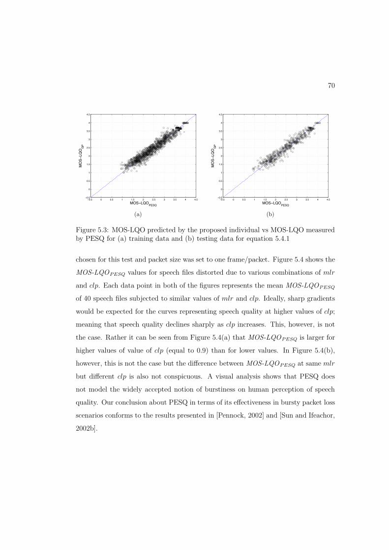
70

−0.5 0 0.5 1 1.5 2 2.5 3 3.5 4 4.5−0.5

0

0.5

1

1.5

2

2.5

3

3.5

4

4.5

MOS−LQOPESQ

MO

S−LQ

OG

P

(a)

−0.5 0 0.5 1 1.5 2 2.5 3 3.5 4 4.5−0.5

0

0.5

1

1.5

2

2.5

3

3.5

4

4.5

MOS−LQOPESQ

MO

S−LQ

OG

P(b)

Figure 5.3: MOS-LQO predicted by the proposed individual vs MOS-LQO measuredby PESQ for (a) training data and (b) testing data for equation 5.4.1

chosen for this test and packet size was set to one frame/packet. Figure 5.4 shows the

MOS-LQOPESQ values for speech files distorted due to various combinations of mlr

and clp. Each data point in both of the figures represents the mean MOS-LQOPESQ

of 40 speech files subjected to similar values of mlr and clp. Ideally, sharp gradients

would be expected for the curves representing speech quality at higher values of clp;

meaning that speech quality declines sharply as clp increases. This, however, is not

the case. Rather it can be seen from Figure 5.4(a) that MOS-LQOPESQ is larger for

higher values of value of clp (equal to 0.9) than for lower values. In Figure 5.4(b),

however, this is not the case but the di!erence between MOS-LQOPESQ at same mlr

but di!erent clp is also not conspicuous. A visual analysis shows that PESQ does

not model the widely accepted notion of burstiness on human perception of speech

quality. Our conclusion about PESQ in terms of its e!ectiveness in bursty packet loss

scenarios conforms to the results presented in [Pennock, 2002] and [Sun and Ifeachor,

2002b].

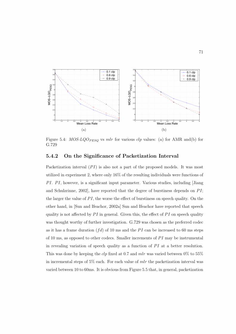
71

1 1.5 2 2.5 3 3.5 4 4.5 5 5.5 61.8

2

2.2

2.4

2.6

2.8

3

3.2

3.4

3.6

3.8

Mean Loss Rate

MO

S−LQ

OPE

SQ

0.1 clp0.6 clp0.9 clp

(a)

1 1.5 2 2.5 3 3.5 4 4.5 5 5.5 61.8

2

2.2

2.4

2.6

2.8

3

3.2

3.4

3.6

Mean Loss Rate

MO

S−LQ

OPE

SQ

0.1 clp0.6 clp0.9 clp

(b)

Figure 5.4: MOS-LQOPESQ vs mlr for various clp values: (a) for AMR and(b) forG.729

5.4.2 On the Significance of Packetization Interval

Packetization interval (PI) is also not a part of the proposed models. It was most

utilized in experiment 2, where only 16% of the resulting individuals were functions of

PI. PI, however, is a significant input parameter. Various studies, including [Jiang

and Schulzrinne, 2002], have reported that the degree of burstiness depends on PI;

the larger the value of PI, the worse the e!ect of burstiness on speech quality. On the

other hand, in [Sun and Ifeachor, 2002a] Sun and Ifeachor have reported that speech

quality is not a!ected by PI in general. Given this, the e!ect of PI on speech quality

was thought worthy of further investigation. G.729 was chosen as the preferred codec

as it has a frame duration (fd) of 10 ms and the PI can be increased to 60 ms steps

of 10 ms, as opposed to other codecs. Smaller increments of PI may be instrumental

in revealing variation of speech quality as a function of PI at a better resolution.

This was done by keeping the clp fixed at 0.7 and mlr was varied between 0% to 55%

in incremental steps of 5% each. For each value of mlr the packetization interval was

varied between 10 to 60ms. It is obvious from Figure 5.5 that, in general, packetization

72

interval has no obvious e!ect on speech quality. The speech quality decreases as the

packet loss rate increases but remains, somewhat, steady across various packetization

intervals.

10 20 30 40 50 60

05

1015

2025

3035

4045

5055

−0.5

0

0.5

1

1.5

2

2.5

3

3.5

4

4.5

Packetization Interval (ms)

MO

S−LQ

OPE

SQ

Mean Loss (%)

Figure 5.5: The values of MOS-LQOPESQ at various values of mlr and packetizationintervals for G.729 codec. The clp was set to 0.7

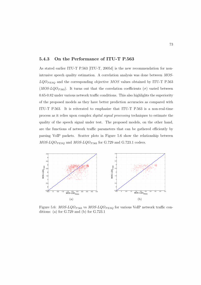
73

5.4.3 On the Performance of ITU-T P.563

As stated earlier ITU-T P.563 [ITU-T, 2005d] is the new recommendation for non-

intrusive speech quality estimation. A correlation analysis was done between MOS-

LQOPESQ and the corresponding objective MOS values obtained by ITU-T P.563

(MOS-LQOP.563). It turns out that the correlation coe"cients (") varied between

0.65-0.82 under various network tra"c conditions. This also highlights the superiority

of the proposed models as they have better prediction accuracies as compared with

ITU-T P.563. It is reiterated to emphasize that ITU-T P.563 is a non-real-time

process as it relies upon complex digital signal processing techniques to estimate the

quality of the speech signal under test. The proposed models, on the other hand,

are the functions of network tra"c parameters that can be gathered e"ciently by

parsing VoIP packets. Scatter plots in Figure 5.6 show the relationship between

MOS-LQOPESQ and MOS-LQOP.563 for G.729 and G.723.1 codecs.

−0.5 0 0.5 1.0 1.5 2.0 2.5 3.0 3.5 4.0 4.5−0.5

0

0.5

1

1.5

2

2.5

3

3.5

4

4.5

MOS−LQOPESQ

MO

S−LQ

OP.

563

(a)

−0.5 0 0.5 1.0 1.5 2.0 2.5 3.0 3.5 4.0 4.5−0.5

0

0.5

1

1.5

2

2.5

3

3.5

4

4.5

MOS−LQOPESQ

MO

S−LQ

OP.

563

(b)

Figure 5.6: MOS-LQOP.563 vs MOS-LQOPESQ for various VoIP network tra"c con-ditions: (a) for G.729 and (b) for G.723.1

74

5.5 A Comparison with other Approaches

In this section the proposed methodology and the derived models are compared with

the other parametric modeling approaches. A detailed comparison with every existing

technique and result is di"cult. Firstly, it is hard to reproduce the simulation results

in exactly the same manner. Moreover, the nature of the training/testing data may

a!ect the research results. Here, for instance, one research study may have assumed

packet losses to be random (i.e. following a Bernoulli loss pattern) whereas another

study may have assumed bursty losses. Similarly, the number of codecs employed

can also have implications towards the performance of the derived models. Based on

this a descriptive comparison is made between the proposed models and the existing

studies.

Sun and Ifeachor [Sun and Ifeachor, 2006] and Rosenbluth [Cole and Rosenbluth,

2001] have proposed logarithmic functions to compute quality degradation functions.

They assume that quality degrades logarithmically as a function of packet loss rate.

There are two principal problems with their approach. First, it is obvious that for

the chosen codecs the quality degradation is logarithmic with respect to the packet

loss rate. However, this assumption may not hold for all codecs; the functional forms

of codecs may di!er from each other. Secondly, they have to tune two additional

variables for each of the coding conditions e.g. for AMR-NB 7.4 and 12.2 (kbps)

modes, two pairs of coe"cients would have to be computed, which would then be

stored in a look-up table or a database. Moreover, the performance results proposed

by Sun and Ifeachor in [Sun and Ifeachor, 2006], despite appearing superior to ours,

have been computed for the case of single coding conditions. Our results generalize

for a wider range of distortion conditions.

Hoene et al. [Hoene et al., 2004] have employed a look-up table based approach

for the derivation of their quality model. For a given codec they store the MOS

75

corresponding to certain values of packet loss rates. If during network operation, a

value of packet loss rate that is not present in the look-up table is observed, linear

interpolation is performed for known values to derive the result. In addition to the

relative complexity of this approach compared to our proposal, the model is limited

to the case of the AMR-NB codec only.

Sun and Ifeachor [Sun and Ifeachor, 2002a], Mohamed et al. [Mohamed et al.,

2001] [Mohamed et al., 2004] have performed disparate research studies which employ

ANNs to derive quality estimation models. A major problem with their approach,

as in various ANN based models, is that a set of redundant variables has been used.

Thus, for instance, [Sun and Ifeachor, 2002a] used mbl as an independent variable

for the computation of the model. However, our research has shown that mbl is

redundant. Our results are comparable to theirs. On the other hand, Mohamed et

al. [Mohamed et al., 2001] [Mohamed et al., 2004] used subjectively estimated MOS as

reference for model derivation. As discussed earlier, subjective estimates are superior

to the results obtained through objective models such as PESQ. Their results are

also seemingly superior to ours. However, there are a number of reasons for this. In

their research they have only used 4–5 discrete values for packet loss rate. We have

employed 12 values, allowing a finer granularity of data. Similarly, they employed

a smaller number of network tra"c configurations. Thus, for instance, where 112

di!erent network configurations were simulated in [Mohamed et al., 2004], we used a

total of 840 network operating conditions; an order of magnitude higher. This includes

various combinations of mlr, mbl, and br etc. Consequently, a smaller number of data

patterns were used both for training and testing. Given that subjective MOS were

used as reference, it may be expected that there would be little variation in the

results due to the prior averaging. Our research employs PESQ, which, for similar

network distortion conditions, may exhibit high variance in results for di!erent speech

samples. Using PESQ as a reference, however, has the advantage that the results can

76

be repeated easily.

5.6 Conclusions

The problem of real-time quality estimation of VoIP is of significant interest. This

chapter has shown an approach for solving this problem by employing GP. One of

the main objectives of this research was to estimate the e!ect of burstiness on speech

quality. It turned out that burst length was least used by the best individuals of

various runs. This is due to the fact that the PESQ algorithm does not model

the e!ect of burstiness on speech quality [Pennock, 2002] [Sun and Ifeachor, 2002b].

Hence, the e!ect of burstiness can be mapped only by conducting suitably designed

formal subjective tests [ITU-T, 1996d]. Despite this limitation, PESQ is the best

objective quality estimation model and has been used to model the e!ect of packet

loss by various studies. The proposed models are good approximations to PESQ

and computationally more e"cient. Hence, they are useful for real-time call quality

evaluation. For the codecs considered in this study, we have also proposed a model

(equation(5.4.2)) that is a function of mlrV AD only with performance comparable to

the other models. This is significant since such a model can be deployed conveniently

on a wide variety of platforms.

Our results are superior to the past research both in terms of performance and

nature of the proposed models. For instance, Sun and Ifeachor [Sun and Ifeachor,

2002a] and Mohamed et. al. [Mohamed et al., 2001] [Mohamed et al., 2004] proposed

ANN based models for VoIP quality estimation with the number of input parame-

ters ranging between 4–5. However, a major limitation of ANNs is that the model

interpretation remains an insurmountable proposition upon successful learning and,

as a consequence, there is no direct method for estimating the significance of various

input parameters. As stated earlier, evolutionary search prunes o! the less significant

77

input parameters leading to simpler models proposed in this Chapter. Similarly, in

their award winning paper Hoene et. al. [Hoene et al., 2004] present a look-up table

based VoIP quality estimation model. The various MOS and corresponding parameter

values would be stored in a lookup table. In the case the table does not contain a par-

ticular value of a parameter, linear interpolation is used to calculate MOS. Moreover,

the model is not developed against a wider variety of input parameters. Although

codec type is suggested as a network tra"c variable in the abstract presentation of

their VoIP quality estimation model, the number of codecs is actually restricted to 1

(i.e. AMR codec) in the model proposed therein. Our proposed models are free from

such limitations. They can be used to assay the VoIP quality for any values of the

input parameters which fall under the permissible range. Moreover, our models have

been evolved against highly varying network conditions.

The focus of this chapter was on estimating speech quality of VoIP in an NB

context. A followup of this research is presented in chapter 6 where equipment im-

pairment factors are derived for the E-Model [ITU-T, 2005a] for a mixed narrow-

band/wideband (NB/WB) context, where distortion conditions due to both NB and

WB codecs exist.

Chapter 6

A Methodology for Deriving VoIPEquipment Impairment Factors fora mixed NB/WB Context

6.1 Introduction

VoIP is curently evolving rapidly towards wideband based transmission. Wideband

(WB) o!ers more natural sounding speech than narrowband (NB), and IP networks

allow the transition to occur essentially by a simple change of codecs. It is clear,

however, that there will be a transitional period, with wideband and narrowband

VoIP coexisting, leading to a requirement for NB/WB interoperation. An important

question that arises as a consequence is how is the quality of such a mixed NB/WB

system to be estimated?

VoIP quality is a!ected by various factors such as packet loss, end-to-end delay,

jitter and codec bit-rate etc. A number of approaches and models exist that estimate

speech quality as a function of such impairments. Of particular interest among these

is ITU-T Recommendation G.107 [ITU-T, 2005a], commonly known as the E-Model,

which is an instrumental model that was initially designed for transmission planning

78

79

purposes. It is based on an impairment factor principle that assumes that the degra-

dations induced by various sources have a cumulative e!ect on speech quality and

that they may accordingly be transformed to a transmission rating scale (R scale).

The E-Model was originally intended for NB speech quality estimation. Recently,

in [Moller et al., 2006], Moller et al. proposed an extension of the R scale to in-

corporate WB codecs into E-Model, while leaving the original R scale for the NB

case intact. Their main emphasis has been on deriving equipment impairment factors

(Ie,WB), in a mixed NB/WB context, that represent the degradation in the listening

quality of speech in the wake of pure codec related distortions. Their derivation is

based on subjective listening only tests [ITU-T, 1996c] for a mixture of various NB

and WB codecs defined by ITU-T.

In the past several authors have taken di!erent approaches towards deriving ef-

fective equipment impairment factors (Ie,eff) for NB codecs. E!ective equipment im-

pairment factors correspond to combined impairments due to packet loss and codec.

In this research a novel perspective was taken towards deriving e!ective equipment

impairment factors for the mixed NB/WB case i.e., Ie,WB,eff . Here the novelty is

twofold. First, we propose to use instrumental models as a means to derive reference

Ie,WB,eff , as opposed to subjective tests. Secondly, the mapping between various

quality a!ecting parameters and reference Ie,WB,eff is achieved by employing Genetic

Programming (GP) based symbolic regression [Koza, 1992]. This approach is based

on the work reported in Chapter 5 (and also in [Raja et al., 2006] and [Raja et al.,

2007]) where GP was used to derive parsimonious speech quality estimation models.

In this research a number of state-of-the-art VoIP telephony codecs proposed by

ITU-T have been employed. ITU-T P.862.2 (i.e.WB-PESQ), as reported in [ITU-T,

2005f], has been used as a reference system. We follow the methodology described

in [ITU-T, 2002] for deriving Ie,eff and propose ours as an addendum to it for deriving

Ie,WB,eff .

80

The rest of this chapter is organised as follows. In section 6.2 the E-model frame-

work is described. There we highlight past attempts by various researchers in deriving

Ie,eff and Ie,WB,eff and present our approach too. Section 6.3 discusses the factors

that a!ect Ie,WB,eff . Section 6.4 elucidates the proposed methodology in detail along

with the VoIP simulation system describing various NB and WB codecs used in this

research and the data processing procedures. Details of GP experiments, various

results and models are discussed in section 6.5. Finally, section 6.6 concludes this

chapter.

6.2 The E-Model

The E-Model, as defined by ITU-T G.107 [ITU-T, 2005a], is a computational model

used for assessing the combined e!ect of various parameters on speech quality in a

conversational sense. Initially it was designed for NB handset telephony, however,

its adaptation to the WB case is currently in progress. The primary output of the

model is the Rating Factor, R. The derivation of R is based on an impairment factor

principle that assumes that factors a!ecting speech quality are additive in nature.

Thus, R is computed according to equation (6.2.1):

R = R0 ! Is ! Id ! Ie,eff + A (6.2.1)

where R ranges from 0 (poor quality) to 100 (optimum quality) for the NB case.

R0 is the basic signal to noise ratio which, for the NB case, defaults to 93.2. Is

represents all the impairments which occur simultaneously with the voice including,

for instance, overall loudness rating and non-optimum sidetone. Id marks the e!ect

of delay related impairments such as echo and too long end-to-end delay that may

a!ect the call quality in a conversational sense. Ie,eff depicts the impairments due to

low bit-rate codecs in the presence of packet losses. Finally, A is the advantage factor

81

that compensates for the above impairment factors when there are other advantages

of access to the user depending on the nature of the underlying network. Thus, for

instance, A may be assigned a value of 0 for a wired network and 20 for a multi-hop

satellite connection. In the case where values of one or more of these factors may not

be determined, default values are used from [ITU-T, 2005a]. Thus, the advantage

factor may be thought to be a convenience whereby the user may be more forgiving

on quality.

R can be converted to Mean Opinion Score (MOS) and vice versa using corre-

sponding transformations given in [ITU-T, 2005a]. Since we have leveraged from

these transformations in this research we shall refer to them by an abstract notation

given by transformation (6.2.2). The related pair of equations is given in appendix A

for perusal.

R '( MOS (6.2.2)

where MOS varies on a scale ranging between 1 (bad) to 4.5 (excellent), and it is a

measure of human assessment of speech quality. The relationship between MOS and

R is shown in Figure 6.1 with the solid curve.

The above formulations hold for the case of NB codecs. In [Moller et al., 2006]

Moller et al. proposed a transformation of the R scale from the NB case (RNB) to the

mixed NB/WB case (RNB/WB) based on subjective tests performed in [Barriac et al.,

2004]. The test results suggest that for the scenario where only NB coded samples

were present, MOS scores were higher than those for the same samples evaluated in

presence of additional, objectively better, WB coded stimuli. Moreover, since the

MOS to R conversion represented by transformation (6.2.2) was applied, the RNB,

for the NB context, turned out to be higher than RNB/WB for the mixed NB/WB

context. This would have repercussions for the validity of the original R scale in

a mixed NB/WB context as it would a!ect the NB usage of the scale. Thus, an

82

0 25 50 75 100 1251

1.5

2

2.5

3

3.5

4

4.5

Transmission Rating Factor R

MO

S

Rmax=129(Moeller et al.)Rmax=100(E−model)Rmax = 107.18(PESQWB)

Figure 6.1: Transformation rules between R and MOS. Solid line: NB case of theE-Model, dashed line, NB/WB case (Moller et al.) and dashed-dotted line forWB-PESQ

extension of the R scale for the NB/WB case was proposed that leaves the original

R scale for the NB context unaltered. This extension is given by equation (6.2.3)1.

Rnew = a.'

eRNB/WB/b ! 1(

(6.2.3)

where a and b were found to be equal to 169.38 and 176.32 respectively, and RNB/WB

can be calculated via (6.2.2). This extension is now an integral part of the E-Model

(see Appendix II of [ITU-T, 2005a]), where the new default value for R0 for the

NB/WB case is 129. Following this, Ie,WB (i.e. impairments solely due to various

1A linear version of this extension also exists that has been skipped for brevity

83

low bit-rate NB/WB codecs) can be calculated according to equation (6.2.4) as a

di!erence between R-value of the direct channel and R-value corresponding to the

codec under consideration.

Ie,WB = 129 ! Rcodec (6.2.4)

where Rcodec may be calculated from (6.2.3) and 129 corresponds to the value of R

for the direct channel for the mixed NB/WB context. The direct channel in this

context is represented by a 16-bit linear PCM with fs=16 kHz (this also assumes

that impairments due to other factors such as echo or delay are not present).

6.2.1 On Extending the R scale for WB-PESQ

Our work employs WB-PESQ as a reference for deriving Ie,WB and Ie,WB,eff , as

opposed to subjective tests. A WB version of R scale does not exist in the literature

for WB-PESQ. There can be two approaches in principle to convert MOS-LQO (MOS-

Listening Quality Objective) [ITU-T, 2003b] obtained by WB-PESQ to the R scale.

Both of these are discussed in this section.

1) One approach may be to extend the R scale using MOS-LQO obtained by

WB-PESQ using the methodology proposed in [Moller et al., 2006] by Moller et al;

as has been previously discussed. Based on this an experiment was performed to see

whether a meaningful extension of the R scale could be made for WB-PESQ. Two

test cases were prepared, each comprising 1328 pairs of reference and coded file pairs

of experiments 1 and 3 of the ITU-T P-series supplement 23 [ITU-T, 1998a]. The

coded files contain various NB scenarios with distortion conditions such as low bit-

rate coding, signal correlated noise, codec tandeming, bit errors and frame erasures.

Conditions representing direct (or clean) NB channel are also present. All the files

are originally coded in 16-bit linear PCM format, fs=16 kHz. The file pairs in the

84

first test case were evaluated with WB-PESQ. This constitutes the WB (or NB/WB)

context with WB coded references and NB coded and upsampled test files. File pairs

in the second test case were evaluated with NB-PESQ. To this end, all the reference

and coded files were downsampled and low-pass filtered using [ITU-T, 2005e] prior to

evaluation. This corresponds to an NB test.

The resulting scatter plot for RNB and RNB/WB is displayed in Figure 6.2. The

data was fitted using least squares regression where a linear relationship of the form

of equation (6.2.5) was used.

RNB = a.RNB/WB + b (6.2.5)

where, a=0.82, b=25.46 and RMSE=4.12.

According to this Rmax was found to be 107.18. This suggests a rather small

extension of the R-scale; only a 7% gain in quality due to WB coded speech. The

new curve is drawn in Figure 6.1 with a dashed-dotted line.

It is worth mentioning here that WB-PESQ has a number of limitations. First of

all, the restricted set of training and testing databases limits the reliability of WB-

PESQ in comparison with NB-PESQ. Language and codec dependence is another

limitation of the algorithm [Raake, 2006, pp-105] [Morioka et al., 2004]. It was also

observed that WB-PESQ systematically underestimates speech quality in comparison

with subjective tests. This was observed from a comparison made between MOS-

LQO obtained by WB-PESQ and MOS-LQS (MOS-Listening Quality Subjective).

The results of the comparison are shown in Figure 6.3. Here the MOS-LQS were

obtained by performing Ie,WB to MOS conversion for codecs under consideration

using equations (6.2.4), (6.2.6)2 and (6.2.2). Values of Ie,WB were taken from [ITU-T,

2006b].

2Equation (6.2.6) is the inverse of equation (6.2.3)

85

Rorig = ln

)

Rnew + 169.38

169.38

*

& 176.32 (6.2.6)

0 20 40 60 80 10020

30

40

50

60

70

80

90

100

110

RNB/WB

R NB

Figure 6.2: Comparison between R-values obtained from a NB and a mixed NB/WBcontext using PESQ.

2) The second approach is to convert the MOS-LQO to the R scale using equations

(6.2.2) and (6.2.3), in the order given. This is analogous to the methodology given in

ITU-T P.834 [ITU-T, 2002]. As there are clear problems associated with reconciling

the R scale in the case of subjective and objective tests, as seen during the analysis

of first approach, we have chosen the second approach. This is used to derive refer-

ence values of Ie,WB,eff in this research. We argue that our methodology would not

be a!ected due to changes in the mathematical form of any R scale extension; the

86

0

0.5

1

1.5

2

2.5

3

3.5

4

4.5

Codec

MO

S

MOS−LQOMOS−LQS

Figure 6.3: Comparison between MOS-LQO and MOS-LQS for various NB and WBcodecs

experiments that follow can be conveniently repeated for a new (target) R scale.

6.3 Ie,WB,eff and Associated Quality Elements

According to the E-Model [ITU-T, 2005a] Ie,eff for a given NB codec may be com-

puted from

Ie,eff = Ie + (95 ! Ie) &Ppl

Ppl

BurstR + Bpl(6.3.1)

where, Ie is the impairment factor for the codec under consideration in the case of no

packet loss. Ppl is the packet loss rate (%). BurstR is the Burst Ratio; discussed below.

Bpl is the packet loss robustness factor for the codec under consideration. It describes

the the robustness of the codec, including the employed packet loss concealment

mechanism, against packet loss. A similar formulation for Ie,WB,eff is given in [Moller

et al., 2006] for random packet loss.

87

Given this, Ie,WB,eff , or equivalently Ie,eff , depends on two quality elements,

namely packet loss and codec. In the text that follows various aspects of these two

elements are discussed in detail.

6.3.1 Packet Loss

Packet loss may either be random, where loss patterns follow a Bernoulli-like distri-

bution, or bursty in nature. In bursty loss, a lost packet tends to exhibit a temporal

dependency on its immediately preceding (lost or arrived) packet, or past n pack-

ets [Raake, 2006] [Sanneck and Carle, 2000] [Jiang and Schulzrinne, 2000] [Clark,

2001]. E-Model defines a BurstR parameter (Burst Ratio) where burstiness is mod-

eled using a two-state Markov model, with a loss and a no-loss state, and with two

transition probabilities associated with each state.

Another factor a!ecting quality impairment, and closely associated with packet

loss, is the packetization interval (PI) (ms), i.e., the payload size of an IP packet.

In order to utilize the transmission bandwidth e!ectively, it is desirable to increase

the PI. However, larger values of PI result in larger transmission delay and possibly

lower speech quality in the event of a packet loss. Current VoIP applications use

values of PI ranging between 10–60 ms as a compromise [Raake, 2006].

The problems associated with packet loss may be circumvented to a certain extent

with various packet loss recovery methods such as Forward Error Correction, Low-

bit-rate Redundancy and Packet Loss Concealment (PLC) [Perkins et al., 1998].

6.3.2 Codec

Ie,WB,eff is a codec specific quantity and thus dependent on it. A speech codec may

either belong to the class of waveform coders, parametric coders or hybrid coders i.e.

a combination of the first two. Waveform coders perform quantization of the speech

88

signal and parametric coders employ a suitable speech production model for reducing

bandwidth requirement for speech transmission [Chu, 2003]. For a given class of

coders the speech quality may further depend on factors such as codec’s bit-rate, frame

size and coding algorithm. The codec’s transmission bandwidth (i.e. NB or WB) also

a!ects the quality perceived by the user. Thus WB codecs deliver better quality than

their NB counterparts mainly because of the increased naturalness of speech due to

the presence of higher order spectral components [Moller et al., 2006] [Raake, 2006].

In the past various authors have tried to model speech quality as a function of

coding bit-rate (in addition to loss metrics) e.g. [Sun and Ifeachor, 2002a] [Mohamed

et al., 2004] [Hoene et al., 2005] and also by the authors in [Raja et al., 2006] [Raja

et al., 2007]. It may be argued that although coding bit-rate may be used as a

quality defining parameter for general predictions, it may not be able to give accurate

predictions due to two main reasons.

First, in the absence of any other impairments two di!erent codecs, with di!ering

bit-rates, may deliver the same quality to users; e.g. G.722 [ITU-T, 1988a] (64 kbps),

G.722.1 [ITU-T, 2005b] (32 kbps) G.722.2 [ITU-T, 2003d] (12.65 kbps) have their

Ie,WB equal to 13 [ITU-T, 2006b].

Secondly, a high degradation of quality may be associated with a codec with low

Ie (or Ie,WB) in the presence of packet loss. An example of this may be AMR-NB

(12.2 kbps) and iLBC (15.2 kbps); the former o!ers a better quality in the absence

of packet losses, whereas the latter outperforms in the presence of losses [Sun and

Ifeachor, 2006]. This behavior is due to the robustness of a codec against packet loss

and may depend on several factors such as , loss distribution (random or bursty),

type of packet loss recovery algorithm employed by the codec and the time taken

by a decoder’s state to resynchronize with that of the coder in the event of packet

loss [Rosenberg, 2001].

This reflects the interpretation that codec-related e!ects on Ie,WB,eff may be due

89

to Ie,WB and the robustness of that codec against packet loss.

6.3.3 Discussion

The E-Model uses two predefined parameters to compute Ie,eff ; namely Ie and Bpl

(packet loss robustness factor) along with packet loss statistics as in equation (6.3.1).

The significance of these parameters has been discussed in section 6.3.2. Similarly,

in [Cole and Rosenbluth, 2001] Cole and Rosenbluth and in [Sun and Ifeachor, 2006]

Sun and Ifeachor have proposed a logarithmic function of the form:

Ie,eff = x1 + x2 & ln(1 + x3 & mlr) (6.3.2)

where they tune xi to compute the codec specific Ie,eff as a function of mean packet

loss rate (mlr). It may be argued that their formulation of Ie,eff depends on Ie (i.e.

when mlr=0) and packet loss robustness, which translates into parameters x2 and x3.

Janssen et al. have depicted a relationship between codec specific Ie,eff and packet

loss rate in the form of quadratic curves [Janssen et al., 2002].

It follows that di!erent codecs may have di!erent curves for Ie,WB,eff . This e!ect

may be seen in Figure 6.4. Here, for example, Ie,WB,eff for the Adaptive Multi-

Rate-NB (AMR-NB) [ETSI, 2000] codec (7.4 kbps) may be approximated with a

logarithmic curve (equation (6.3.2)), whereas the best fit curve for G.722.2 (19.85

kbps) was found to be a 4th order polynomial.

It is clear that currently there is no widely accepted and clearly superior formu-

lation for Ie,WB,eff . We suggest an alternative, altogether di!erent, strategy. Instead

of approaching the problem with a priori assumptions about the analytical form of

Ie,WB,eff , we allow the data to speak for themselves. We propose to evolve high-

quality expressions for Ie,WB,eff using GP.

90

0 5 10 15 20 25 30 35 4020

30

40

50

60

70

80

90

100

110

120

mean loss rate (mlr) %

I e,W

B,ef

f

G.729 (8)G.723.1(6.3)AMR−NB (7.4)G.722.2 (19.85)G.722.1 (32)

Figure 6.4: Ie,WB,eff as a function of mlr for various NB/WB codecs. values forIe,WB,eff were computed using WB-PESQ with random packet loss and PIs equal toone speech frame of the respective codecs.

6.4 The new Methodology

In what follows we first describe our methodology for deriving Ie,WB,eff as a function

of VoIP tra"c parameters. Next, we list the details of our data preparation procedure

and of the VoIP simulations undertaken.

6.4.1 Methodology

This methodology is based on the research presented in 5 (and in [Raja et al., 2006]

and [Raja et al., 2007]), with the main di!erence being that there the objective

91

Speech Database

Model Evolved By GP

Paremeter Extraction

Decoder Loss Simulator Encoder

Quality Measure

(WB-PESQ)

Reference speech signal

Evolved I e,WB,eff

Degraded speech

Target I e,WB,eff

VoIP Traffic parameters

MOS=>R=>R new =>I e,WB,eff

Figure 6.5: Simulation system for derivation of Ie,WB,eff

was to compute MOS for an NB context whereas here the main focus is on deriving

equipment impairment factors, Ie,WB,eff , for a mixed NB/WB context. The schematic

in Figure 6.5 depicts a conceptual diagram of our approach for deriving Ie,WB,eff

for VoIP. An initial requirement is to have a database consisting of clean speech

signals. These signals are subjected to degradations typical of VoIP tra"c; coding

distortions and packet loss. The degraded VoIP stream is eventually converted back

to linear PCM format using a decoder corresponding to the encoder. In the process

of doing so the values of various VoIP tra"c parameters, such as packet loss rate, are

calculated and the decoded speech signal is sent to a viable instrumental model that

may report its results in terms of human assessment of speech quality i.e. MOS-LQO.

Moreover, the model should be able to evaluate both NB and WB coded speech. An

example of such a model is WB-PESQ, which has been used as a reference system

in this research. The resulting MOS-LQO is converted to Ie,WB,eff using equations

(6.2.2), (6.2.3) and eventually (6.2.4). We call this the target Ie,WB,eff . The process

is repeated for a large number of speech signals with varying degrees of network

distortion conditions. Once the target Ie,WB,eff for all the speech signals have been

computed and the values of corresponding VoIP network tra"c parameters gathered,

GP based evolution is performed to derive a suitable mapping. More specifically, the

VoIP network tra"c parameters serve as the input domain variables during evolution

92

and the corresponding Ie,WB,eff values form the target output values.

A linear interpolation between the Ie,WB obtained by the instrumental model (WB-

PESQ) and subjective tests may be performed as suggested by ITU-T P.834 [ITU-T,

2002, pp-9] to adjust the target Ie,WB,eff . To this end, interpolation was performed

between Ie,WB values for 20 (14 WB and 6 NB) codecs obtained using WB-PESQ,

and from subjective tests reported in [ITU-T, 2006b]. Here, for each codec, Ie,WB

corresponding to WB-PESQ was obtained by averaging the evaluations of 30 speech

file pairs. Clean speech files were taken from experiment-1 of [ITU-T, 1998a]. The

slope and intercept were found to be equal to 0.6730 and 35.7881 respectively. It must

be noted that a large intercept indicates an experimental bias [ITU-T, 2001a, pp12].

This is possibly due to the fact that WB-PESQ underestimates the speech quality as

compared with subjective tests, as discussed in section 6.2.1.

6.4.2 Input Domain Variables

mlr, PI and mean burst length (mbl) were chosen as the input domain variables re-

lated to packet loss. Ie,WB and a coarse estimate of loss robustness factor were com-

puted for each codec separately as other independent parameters. It was expected

of GP to make e"cient use of these parameters during evolution. It was discussed

in section 6.3.3, and shown in Figure 6.4, that the functional form of Ie,WB,eff may

vary for di!erent schemes and codecs. Given this, the gradient of Ie,WB,eff for mlr

ranging between 0–0.3 was computed according to equation (6.4.1) as a coarse es-

timate of packet loss robustness factor, assuming that GP would use it e!ectively

during evolution. This range of mlr is chosen because Ie,WB,eff varies the most for

mlr=0.0–0.3. After this the change is only gradual, as can be seen from Figure 6.4.

Moreover, the data presented by Sun and Ifeachor [Sun and Ifeachor, 2006] imply the

same for Ie,eff , where maximum mlr=0.3.

93

grad =Ie,WB,eff(mlr = 0.3) ! Ie,WB,eff(mlr = 0.0)

0.3(6.4.1)

Values of Ie,WB and gradients of Ie,WB,eff with respect to mlr for the codecs under

consideration are listed in Table. 6.1.

Table 6.1: Values for Ie,WB and coarse estimates of loss robustness factorCodec bit-rate Ie,WB gradientG.722.1 32 26.12 216.88G.722.1 24 29.04 208.36G.722.2 6.6 68.13 104.25G.722.2 8.85 58.64 139.67G.722.2 12.65 43.91 187.62G.722.2 14.25 41.19 196.13G.722.2 15.85 39.59 201.50G.722.2 18.25 36.09 212.81G.722.2 19.85 34.97 213.20G.722.2 23.05 32.09 225.27G.722.2 23.85 33.88 221.27G.729 8 62.33 125.66G.723.1 6.3 55.27 142.14AMR-NB 7.4 63.9 151.30AMR-NB 12.2 54.12 187.48

6.4.3 VoIP Simulation

A simulation based approach was pursued in this research, where distortions typical

of a VoIP network were induced on a large number of clean speech signals before de-

coding the corresponding coded bitstreams. Clean speech samples from experiments

1-A and 1-D of ITU-T P-series supplement 23 were used. The NB codecs include:

ITU-T G.729 CS-ACELP (8 kbps) [ITU-T, 1996a], ITU-T G.723.1 MP-MLQ/ACELP

(5.3/6.3 kbps) [ITU-T, 1996b] and AMR-NB codec [ETSI, 2000]. AMR-NB was used

in its 6.7 and 12.2 kbps modes whereas G.723.1 was used in its 6.3 kbps mode.

94

The WB codecs include ITU-T G.722.1 [ITU-T, 2005b] (24/32 kbps) and ITU-T

G.722.2 [ITU-T, 2003d], Adaptive Multi-Rate (AMR-WB) codec. AMR-WB can op-

erate in 9 di!erent coding/decoding modes, each targeting a di!erent bit-rate: all the

coding modes were utilized in this research.

Various network tra"c simulation conditions were chosen in the light of ITU-

T Recommendation G.1050 [ITU-T, 2005c], which specifies a model for evaluating

multimedia transmission performance over an IP network. Bursty packet loss was

emulated using a 2-state Markov model; with probabilities p, for transitioning from

a no-loss state to a loss state and q, for the converse. It was assumed that jitter also

maps to packet loss and that it can be modeled using this 2-state model as in [Sun and

Ifeachor, 2002a]. Packet loss for twelve di!erent values of (target) mlr was simulated;

[0,2.5,. . . , 15, 20, . . . , 40]%. For each value of mlr, conditional loss probability (clp)

(i.e. 1-q) was set to 10, 50, 60, 70 and 80%. It is worth mentioning that higher

values of clp model higher degrees of loss burstiness and vice versa. Moreover, PI

(packetization interval) was varied between 10–60 ms.

Since the clean speech samples are coded at a 16 kHz sampling rate, they were

downsampled before encoding in the case of NB codecs. Subsequently, the corre-

sponding decoded speech samples were upsampled before evaluation by WB-PESQ.

In all, 2,820 combinations of network distortion conditions were emulated. A

given combination of network distortion conditions was applied to four speech sam-

ples. Moreover, each speech sample under consideration was subjected to the same

combination of network distortion conditions 30 times to produce as many test sam-

ples by pseudo-randomly generating di!erent loss patterns each time. This was done

to negate the e!ect of packet loss locations as in [Sun and Ifeachor, 2006] by even-

tually aggregating the MOS for all test samples corresponding to one source sample.

Thus, a total of 338,400 distorted speech files were created. These distorted speech

files were subsequently evaluated by WB-PESQ on a Beowulf cluster with respect

95

to corresponding reference files. Values of the network tra"c parameters for all files

and the corresponding MOS were averaged to form a total of 11,280 input/output

patterns, that would later be utilised during symbolic regression.

6.5 Experiments and results

6.5.1 Experimental Details

Two GP experiments were performed to evolve models for Ie,WB,eff using the in-

put/output data patterns. The accumulation of data patterns has already been dis-

cussed in section 6.4.3. GPLab was used for evolution. Previously in Chapter 5

( [Raja et al., 2007]) we performed four GP experiments with di!erent maximum

tree depths and error measures with di!erent results. In this work we chose the ex-

perimental conditions that produced superior results in terms of quality to perform

the two GP experiments. The common parameters of both experiments are listed in

Table 6.2.

In both experiments scaled mean squared error (MSEs) was used as the fitness

criterion discussed earlier in section 4.3 and given by equation (6.5.1).

MSEs(y, t) = 1/nn

"

i

(ti ! (a + byi))2 (6.5.1)

where y is a GP evolved function of the input parameters in this case (a mathematical

expression), yi represents the output value produced by y for the input case i and ti

represents the corresponding target value of Ie,WB,eff . a and b adjust the slope and

y-intercept of the evolved expression to minimise the squared error.

Tournament selection with Lexicographic Parsimony Pressure (LPP) [Luke and

Panait, 2002] was used in both experiments. Moreover, the selection criteria in

both the experiments was also adapted to the one proposed by Gustafson et al.

96

Table 6.2: Common GP Parameters among all experimentsParameter ValueInitial Population Size 300Initial Tree Depth 6Selection LPPTournament Size 2Genetic Operators Crossover and Subtree MutationOperators Probability Type AdaptiveInitial Operator probabilities 0.5 eachSurvival Half ElitismGeneration Gap 1Function Set plus, minus, multiply, divide,sin,

cos, log2, log10, loge, sqrt,power

Terminal Set Random real-valued numbersbetween 0.0 and 1.0. Integers(2-10). mlr, mbl, PI, Ie,WB, grad

in [Gustafson et al., 2005] for symbolic regression problems.

Whenever input values outside the domain of the functions log, sqrt, division

and pow are encountered, NaN (undefined) values are generated. This results in the

individual concerned being assigned the worst possible fitness value and minimising

its chances of being selected as a parent.

As mentioned in section 4.1, it is typical to conduct several independent runs of

GP. In this case, both experiments entailed 50 independent runs each spanning 50

generations.

The only di!erence between the two experiments was that in the first experiment

the maximum tree depth was 17. This was reduced to 7 in the second experiment

to see if parsimonious individuals with performance comparable to those of the first

experiment can be obtained.

97

6.5.2 Results and Analysis

Of 11,280 input/output patterns reported in section 6.4.3, 1,440 patterns correspond-

ing to AMR-NB 7.4 kbps and G.722.1 32 kbps were separated for model validation on

unseen codecs. Of the remaining 9,840 patterns, 70% were used for training and 30%

for testing the evolved models. Various VoIP tra"c parameters have been discussed

in section 6.4.3. More specifically, these include, Ie,WB, mlr, PI, mean burst length

(mbl) and grad, as in equation (6.4.1), as a coarse estimate of codec specific loss

robustness factor.

The statistics pertaining to RMSEs (square root of the scaled MSE) of training

and testing data of both GP experiments are listed in Table 6.3(a). The table also

lists various statistics related to the tree sizes of GP individuals, in terms of the

number of nodes. The results of both experiments in the final generations were also

treated to a Mann-Whitney Wilcoxon test to assay the significance of di!erences

in various respects. The significance analysis is reported in Table 6.3(b) where a

value of ‘1’ confirms a significant di!erence, at a 5% confidence level, whereas a ‘0’

implies otherwise. It was found that the overall results of the two experiments are

not significantly di!erent from each other in terms of fitness over training and testing

data. However, the di!erence in terms of tree size is significant, with experiment 2

having individuals with smaller trees.

It is also worth mentioning here that the best individuals resulting from three

runs of experiment 1 were treated as over-fit due to their very large RMSEs over the

testing data, ranging between 650–10,000, and were subsequently removed from the

analysis.

In this chapter we present three models resulting from the experiments. Two of

these correspond to individuals with minimum RMSEs over the testing data in each

of the experiments. These are represented by equations (6.5.2) and (6.5.3) and they

98

Table 6.3: Statistical analysis of the GP experiments and derived models(a) MSE Statistics for Best Individuals of 50 Runs for Experiments 1 & 2

Experiment1 Experiment2Stats RMSEtr RMSEte Size RMSEtr RMSEte SizeMean 8.9478 32.5851 28.3617 8.9861 23.9743 19.02Dev. 0.1890 113.2837 12.2144 0.2740 105.2397 6.3326Max. 9.3624 655.5639 77 9.8275 753.2457 38Min. 8.3941 8.5057 13 8.3552 8.4605 10

(b) Results of Mann-Whitney-Wilcoxon SignificanceTest

Experiment1RMSEtr RMSEte Size

Experiment2 0 0 1

(c) Performance Statistics of the Proposed Models

Training TestingModel RMSEs MOS RMSEs Ie,WB,eff ! RMSEs MOS RMSEs Ie,WB,eff !Equation (6.5.2) 0.0990 8.3941 0.9236 0.1007 8.5057 0.9240Equation (6.5.3) 0.0975 8.3552 0.9243 0.0990 8.4605 0.9248Equation (6.5.4) 0.1183 9.1749 0.9080 0.1207 9.3145 0.9080

99

belong to experiments 1 and 2 respectively. The third model, represented by equation

(6.5.4) corresponds to the most parsimonious individual of both the experiments and

is derived from experiment 2.

Ie,WB,eff = (6.5.2)

{11 ! mbl + ln(grad) + grad & mlr + Ie,WB

!2.log2(PI)}& 0.8619 + 9

Ie,WB,eff = (6.5.3)+

ln

)

9 & (Ie,WB + mlr & grad2)

mbl5 ! mlr

*

+ mlr + Ie,WB

+grad & mlr}& 0.8303 + 8.9977

Ie,WB,eff = (6.5.4)

(log10(log10(log2(Ie,WB ! 2 & mbl) + mlr)))

&321.7017 + 95.3708

The RMSEs and Pearson’s product moment correlation coe"cient ("), corre-

sponding to Ie,WB,eff for these models are compared with each other in Table 6.3(c).

The values of RMSEs corresponding to MOS-LQO are also listed as another com-

parison. These were computed by converting the target values of Ie,WB,eff and those

obtained by the models under consideration to the MOS scale. This may be done

by obtaining the values of R corresponding to Ie,WB,eff from equation (6.2.4). The

result can then be transformed to the original R scale for the NB-only context using

equation (6.2.6); the inverse of equation (6.2.3). The resulting values of R can be

100

converted to the MOS scale using transformation (6.2.2). The significance of all of

the models can be judged by observing that the values of RMSEs on the MOS scale

in all cases range between 0.098–0.12. This presents a considerably minute di!erence

for a human subject to detect.

Equation (6.5.3) has the best statistics among all. Figure 6.6 shows the scatter

plots of equation (6.5.3) versus WB-PESQ, where it can be seen that the data points

produced by both are firmly glued to the 45 degrees reference line.

0 20 40 60 80 100 120 1400

20

40

60

80

100

120

140

Ie,WB,eff−WB−PESQ

I e,W

B,ef

f−G

P

(a)

0 20 40 60 80 100 120 1400

20

40

60

80

100

120

140


I e,W

B,ef

f−G

P

(b)

Figure 6.6: Ie,WB,eff predicted by equation (6.5.3) vs target Ie,WB,eff for: (a) trainingdata (b) testing data

A significance analysis of the various VoIP tra"c parameters, in terms of their

appearance in the best individuals of 50 runs of each of the two experiments, was

done. The results are graphed in Figure 6.7. According to this Ie,WB and mlr

had the highest utility, and appeared in 92–94% of the individuals. The third most

101

significant parameter was grad, appearing in 36–38% of the best individuals of both

experiments. mbl appeared in between 24–26% whereas, PI appeared in only 12%

of the best individuals. The last two observations have also been reported by other

researchers, such as [Sun and Ifeachor, 2002b] [Pennock, 2002], who note that PESQ

does not model the e!ect of burstiness on speech quality. We reported similar results

in Chapter 5 and in [Raja et al., 2006]. Figure 6.8 illustrates similar behavior, but for

WB-PESQ and a WB codec (AMR-WB 23.85 kbps). It is obvious that a correlation

between Ie,WB,eff and mbl does not exist. A similar comparison for the case of G.729

is shown in Figure 6.9 where absence of any correlation between Ie,WB,eff and PI

may also be observed.

Experiment 1 Experiment 20

20

40

60

80

100

Ie,WBgradmlrPImbl

Figure 6.7: Percentage of the best individuals employing various input parameters inacceptable runs of each of the two experiments.

6.5.3 Comparison with the E-Model

Finally, a comparison of equation (6.5.3) was made with the E-Model’s formulation

of the Ie,WB,eff , as in [Moller et al., 2006]. This is represented by:

102

0....

40

0

20

40

60

80

100

120I e,

WB,

eff

% Packet Loss

mbl

Figure 6.8: Variation of Ie,WB,eff against mlr (%) and mbl = [1, · · · , 5] for AMR-WB23.85 kbps, PI=1.

Ie,WB,eff = Ie,WB + (129 ! Ie,WB) &Ppl

Ppl + Bpl(6.5.5)

The equation is similar to equation (6.3.1) di!ering in the constant term, 95, which

is replaced with the new Rmax=129. The BurstR parameter is also absent here.

Bpl values for this equation were computed separately for each of the codecs over

the training data, and the performance was analysed using the testing data. Loss

distributions were assumed to be random, which may be thought to be a reasonable

103

0 2.5. . . .

1210 . . .

60

0

50

100

150

PI (ms)

I e,W

B,ef

f

% Packet Loss

Figure 6.9: Variation of Ie,WB,eff against mlr (%) and PI = [10, · · · , 60ms] for G.729

assumption since it was shown in Figures 6.8 and 6.9 that WB-PESQ estimates are

oblivious of the e!ect of burstiness and varying PIs. The results are reported in

Table 6.4 for each codec. The table also shows the RMSE of equation (6.5.3) for

AMR-NB (7.4 kbps) and G.722.1 (32 kbps). These codecs were not represented in

the training data during evolution. Percentage Prediction Gain (PG) of 16.36 % was

observed for unseen data in an RMSE sense. This is calculated according to equation

(6.5.6)

%PG =RMSEe ! RMSEp

RMSEe& 100 (6.5.6)

where, RMSEe and RMSEp represent the RMSE of equations (6.5.5) and (6.5.3)

respectively.

104

However, equation (6.5.5) (i.e. the E-model formulation) does not account for

bursty packet losses and also for PI spanning multiple speech frames. Moreover,

all the models proposed in this research (by equations (6.5.2)–(6.5.4)) are functions

of mbl. Given this, a comparison between E-model and the proposed models over

datasets that include various degrees of burstiness and PIs is somewhat unfair. To

ensure fairness a di!erent simulation study was performed in which speech files were

subjected to random packet losses with loss rates ranging between [0,2.5,. . . , 15, 20,

. . . , 40]% for each of the encoding conditions. The results are reported in Table 6.5.

To this end, the data was split into training and testing datasets as previously. Bpl

values were recalculated for each of the codecs and the RMSE was noted with respect

to WB-PESQ. The performance of equation (6.5.3) was found to be inferior to the

traditional E-model formulation initially. Since random loss conditions were alien to

the GP training conditions, the performance degradation was not unexpected when

compared to a retuned E-model. However, upon merely re-scaling equation (6.5.3)

using training data a prediction gain of approximately 36% was obtained. This shows

the robustness of the model produced by GP as evolutionary re-training was not

required. Linear re-scaling resulted in new slope and intercept terms which were

found to be 0.5085 and 46.7468 respectively. Linear re-scaling was done by treating

equation (6.5.3) with equations (4.3.2) and (4.3.3). A pictorial comparison similar

to Figure 6.6 is also done between equations (6.5.3) and (6.5.5) with respect to WB-

PESQ in Figure 6.10 for the case of ITU-T G.723.1 codec. It can be observed that

the points produced by equation (6.5.3) are more firmly glued to the 45% reference

line as compared to those produced by equation (6.5.5).

105

Table 6.4: Comparison between the Prediction Accuracies of the E-Model and theProposed Model

E-Model Equation (6.5.3)Codec RMSE RMSE RMSE RMSE(kbps) Bpl train test train testG.722.1 (24) 20.32 8.6824 8.8958 8.1701 8.9118G.722.2 (6.6) 40.75 9.6225 8.9933 8.0938 7.6603G.722.2 (8.85) 28.74 10.0175 9.9919 8.0185 7.8304G.722.2 (12.65) 21.58 10.5538 10.4088 8.2188 8.0678G.722.2 (14.25) 21.03 10.4684 11.2854 8.3031 8.5836G.722.2 (15.85) 19.98 10.599 11.5020 8.3257 9.1166G.722.2 (18.25) 19.48 11.2017 10.92 8.6862 9.0266G.722.2 (19.85) 18.86 10.5502 11.3529 8.2338 8.7685G.722.2 (23.05) 18.44 11.4079 11.1663 9.1417 8.7729G.722.2 (23.85) 17.92 10.789 11.1948 8.6125 9.3168G.729 (8) 28.43 8.95 9.1631 7.3888 7.4943G.723.1 (6.3) 29.19 10.83 10.3630 8.8116 8.5259AMR-NB (12.2) 13.50 8.0689 7.2947 9.4549 8.7322

G.722.1 (32) 18.93 8.9112 – – 8.4775AMR-NB (7.4) 15.71 7.1335 – – 8.6188

Average – 9.8527 10.1946 8.42 8.5269% PG – – – 14.54 16.36

6.6 Conclusions

In this Chapter we have proposed a novel methodology for determining NB/WB

equipment impairment factors, Ie,WB,eff , for a mixed NB/WB context. It is based

on using GP to perform symbolic regressions which generate simple formulae for

Ie,WB,eff . It is advantageous in the sense that the derived models do not result from

human bias, but as a direct consequence of program evolution. Moreover, parameter

optimization is done in parallel with evolution for every model using linear scaling.

The derived models are applicable for the network distortion conditions under obser-

vation. Our approach utilizes WB-PESQ for deriving reference values of Ie,WB,eff as

opposed to subjective tests. This is suitable for fast and inexpensive derivation of

106

Table 6.5: Comparison between the Prediction Accuracies of the E-Model and theProposed Model for Random Loss Conditions

E-Model Equation (6.5.3) Equation (6.5.3)After Rescaling

Codec RMSE RMSE RMSE RMSE RMSE RMSE(kbps) Bpl train test train test train testG.722.1 (24) 11.97 12.2622 13.1168 14.9678 14.8504 6.6551 6.9227G.722.2 (6.6) 24.06 8.5488 8.5060 8.2690 7.8553 6.9593 7.2537G.722.2 (8.85) 14.61 9.7573 9.8179 11.2923 11.3162 5.9292 6.2118G.722.2 (12.65) 10.62 11.2011 11.2734 14.4629 14.7035 6.6388 6.7783G.722.2 (14.25) 10.01 11.2489 11.1616 15.0003 14.8100 6.2532 6.5631G.722.2 (15.85) 9.90 11.7606 12.1703 15.5678 15.6983 6.4557 6.9346G.722.2 (18.25) 9.36 12.3315 12.7594 16.5918 17.0715 6.9336 7.3102G.722.2 (19.85) 9.06 12.3594 12.1367 16.8570 16.8927 6.9994 6.9165G.722.2 (23.05) 8.37 13.1165 12.9824 18.1885 17.9847 7.1816 7.3181G.722.2 (23.85) 8.52 12.6131 12.4198 17.7068 17.3806 7.0750 6.6818G.729 (8) 16.82 8.5228 8.7014 9.6080 9.7882 5.5697 5.5535G.723.1 (6.3) 14.95 9.5020 10.3181 10.7527 11.1905 6.4791 6.6315AMR-NB (12.2) 5.76 8.6698 8.3887 17.9201 18.4502 9.2798 9.6566

G.722.1 (32) 11.69 14.0378 13.6078 16.3347 15.7470 7.4048 7.8482AMR-NB (7.4) 7.59 7.8755 8.5562 14.7356 14.7646 7.8499 7.7822

Average – 10.9205 11.0611 14.5504 14.5669 6.9109 7.0909% PG – – – -33.2393 -31.6949 36.7163 35.8934

reference Ie,WB,eff . We have demonstrated the utility of our approach by generating

three models for Ie,WB,eff from di!erent GP runs. The proposed models were thor-

oughly tested on a wide variety of VoIP tra"c scenarios including a blend of modern

IP telephony codecs.

A comparison of equation (6.5.3), which has the best performance among the

proposed models, with the E-Model, equation (6.5.5), has also been done, where it is

shown that our approach outperforms the E-Model with a significant margin in terms

of prediction accuracy. Even though we have used WB-PESQ in this research, the

proposed methodology is independent of it and simply requires a generic instrumental

model of this kind. The methodology may also be augmented with subjective tests.

107

0 20 40 60 80 100 120 1400

20

40

60

80

100

120

140


I e,W

B,ef

f−O

ther

Mod

els

Reference LineE−ModelEquation 13after rescaling

(a)

0 20 40 60 80 100 120 1400

20

40

60

80

100

120

140


I e,W

B,ef

f−O

ther

Mod

els

(b)

Figure 6.10: Ie,WB,eff predicted by equation(6.5.5) (i.e. the E-Model) and equation(6.5.3) vs target Ie,WB,eff obtained from WB-PESQ for random loss: (a) trainingdata (b) testing data.

Chapter 7

Real-Time, Non-Intrusive SpeechQuality Estimation: ASignal-based Model

7.1 Introduction

Chapters 5 and 6 introduced parametric models for speech quality estimation. Some-

times, however, it becomes incumbent to employ a signal-based model to estimate

speech quality. Firstly, signal-based models are applicable to a wider variety of net-

works than parametric ones1. Moreover, in the case of VoIP, there are certain types of

network distortions whose impact on speech quality cannot be measured using para-

metric models. For instance, during transmission over WLANs speech frames may

undergo bit-errors whose e!ect on perceptual quality may not be measurable using a

parametric model. Similarly, the asymmetry of distortions in the case of transcoding

was discussed in Section 2.4.5. Quality degradation while the speech signal traverses

multiple codecs in a given order may not necessarily be the same for a di!erent order.

It is due to such reasons that parametric models may give false predictions on speech

1Since parametric models are designed for a particular type of communications network, theirpredictions for that type of network are more accurate than those of signal-based models; signal-based models are suitable for general predictions for a wider variety of networks.

108

109

quality. Signal-based models may be more useful in such scenarios.

Signal-based models are used to analyze speech quality when the spectral envelope

of the speech signal may have su!ered from degradation. Considerable work has been

done in the past on devising signal-based models. An example of such a model is the

current, state-of-the-art, ITU-T Recommendation P.563 for single-ended estimation

of speech quality [ITU-T, 2005d].

In this chapter we propose a new non-intrusive signal-based model for speech

quality estimation in a narrowband (NB) context. In particular we have employed a

hybrid optimization approach that uses Genetic Programming (GP) to search for a

suitable structure for the desired solution. Coe"cients of the models evolved by GP

are tuned simultaneously using a Genetic Algorithm (GA) and linear scaling. The

use of hybrid optimization is novel here when compared to chapters 5 and 6.

The rest of this Chapter is organized as follows. Section 7.2 discusses the nature

of signal based models. Section 7.3 discusses the various experimental details and

test results. Finally section 7.4 presents the conclusion.

7.2 Signal Based Non-Intrusive Models

Unlike parametric models, signal-based models process the audio stream to extract

the information relevant to distortions in a signal. The estimated distortions are

then converted into MOS estimates for that audio stream. Given this, a signal

based model may have two main modules. 1) A feature extractor that processes the

speech signal and extracts cogent distortion indicators. To this aim, various speech

processing algorithms have been devised for feature extraction. 2) A mapping module

that transforms the extracted features into MOS estimates. In what follows, some of

the well known algorithms that have been used in the past for both feature extraction

and MOS mapping are briefly described.

110

7.2.1 Feature Extraction Algorithms

Feature extraction algorithms may involve time and/or frequency domain analysis

of the speech signal under test. Time domain analysis may involve computation of

distortions relevant to the waveform of the speech signal. Some distortions of this

type include temporal clipping, level variation and abrupt changes in the temporal

envelope of the signal.

Frequency domain analysis techniques normally emulate the human vocal produc-

tion system [Gray et al., 2000], or the auditory processing system of the human ear.

Perceptual Linear Prediction (PLP) [Hermansky, 1990] is one of the exemplary algo-

rithms for speech processing and feature extraction. It was first employed by [Liang

and Kubichek, 1994] Liang and Kubichek in 1994 for non-intrusive speech quality

estimation. It was originally developed for speaker independent automatic speech

recognition and is an emulation of the human auditory system.

ITU-T Recommendation P.563 [ITU-T, 2005d] is the current standard for signal-

based non-intrusive speech quality estimation. It entails a rigorous feature extraction

process that involves the computation of plausible features from both time and fre-

quency domain representations of the signal under test. The algorithm has been

discussed in section 3.3.3.

7.2.2 Mapping Algorithms

Once cogent features corresponding to the speech signal under test have been ex-

tracted, they are mapped to the speech quality using an appropriate regression or

classification tool or a machine learning algorithm. Thus, for training a model nu-

merous MOS-labelled speech databases are used. An MOS-labelled speech database

may have a considerable number of speech samples from both male and female speak-

ers, and possibly in di!erent languages. The duration of each speech sample may vary

111

from 8-12 secs. Each speech sample may be a!ected by a certain type of network dis-

tortion, such as frame erasure, bit errors and/or signal correlated/uncorrelated noise.

Each sample also has a MOS score associated with it, derived normally from sub-

jective tests [ITU-T, 1996c]. The features relevant to distortions for all the samples

serve as the input domain variables and the corresponding MOS scores form the tar-

get values for learning. After learning completes, the derived model is also tested and

validated using unseen data from a separate set of speech samples/databases, as a

standard practice.

Numerous learning algorithms have been used in the past to map the e!ect of

speech features, and/or their relevant statistics, to speech quality. Depending upon

the learning algorithm the training and mapping procedures may vary. One approach

is to compute a significant number of feature vectors corresponding to clean, distor-

tion free, speech files. A database of clean speech feature vectors may be formed

by classifying the latter into clusters to form a reference code-book. An appropriate

vector quantization algorithm such as K-means, as in [Jin and Kubichek, 1996], or

self organizing maps, as in [Picovici and Mahdi, 2004], may be employed. As a part of

training, feature vectors corresponding to distorted speech samples are extracted and

their distances are computed from the best matching feature vector in the reference

code-book in a Euclidean sense. These auditory distances are eventually mapped to

reference MOS scores using a 2nd or a 3rd order polynomial. An obvious limitation

of such an approach is the time required to search for a best matching vector from

the reference code-book of feature vectors of clean speech. Another approach is to

map the feature vectors of the training speech samples directly to speech quality

using an artificial neural network [Tarraf and Meyers, 1999]. In [Falk and Chan,

2006] Falk and Chan have used Gaussian mixture models (GMMs), support vector

classifiers and multi adaptive regression splines at various stages of their proposed al-

gorithm to map the cogent features to speech quality. Similarly in [Grancharov et al.,

112

2006] Grancharov et al. also employed a GMM for speech quality prediction. In [Li

and Kubichek, 2003] Li and Kubichek employed a hidden Markov model (HMM)

for mapping the speech related features to quality. Among all of these algorithms

HMMs attempt to explore statistical dependencies between adjacent segments of hu-

man speech, whereas for the rest of the algorithms aggregated values of features over

the entire length of a speech signal are used.

ITU-T performs perceptual mapping between the features of speech signal under

test and the speech quality. The mapping process has already been discussed in

section 3.3.3.

7.2.3 The Proposed Model

This chapter proposes a new model for speech quality estimation. We have used P.563

as the feature extraction algorithm in this research. This has been chosen for two

reasons: 1) P.563 is the current, state-of-the-art standard for non-intrusive speech

quality estimation. 2) it computes the most numerous and most varied features

relevant to speech quality than any other feature extraction algorithm. However,

for mapping the features to speech quality we have employed a GP based symbolic

regression approach, along with a traditional GA, and linear scaling as proposed by

Keijzer in [Keijzer, 2004], for parameter optimization. GP is used to evolve a suitable

structure for mapping the features to speech quality. As described in Chapter 4 GP

is also known to prune o! the redundant features and to retain the most useful ones

in the genome of the final individual. The GA is employed to fine tune the numeric

leaf values during evolution.

113

7.3 Experiments and Results

7.3.1 Experimental Setup

As a first step feature extraction was performed by processing various MOS labeled

speech databases using the P.563 algorithm. A total of eight subjectively evalu-

ated speech databases were used in this research. Out of these, seven multilingual

databases belong to the ITU-T P-series supplement 23 (Experiments 1 and 3) [ITU-T,

1998a]. These databases include 1328 speech samples distorted due to conditions such

as signal correlated noise, transcoding, bit errors and frame erasures. The databases

include utterances by male and female speakers. The eighth database includes 240

utterances in the North American English accent by two male and two female speak-

ers with seven types of distortion conditions. This database is compiled by Nortel

Networks [Thorpe and Yang, 1996]. The distortion conditions, each of varying levels,

include signal correlated noise, coding distortions, tandeming, temporal clipping, bit

errors and speech level variation. 70% of the speech files, and their corresponding

MOS, in these databases were dedicated for training and the remaining 30% for test-

ing reasons. More specifically, input/output patterns of 1,100 speech files were picked

randomly as training data, and the remaining, 468 patterns were used for the purpose

of testing.

Values of 43 features corresponding to each of the speech files were accumulated as

the input domain variables. The corresponding MOS scores formed the target values

for training and testing the evolutionary experiments.

Three GP experiments were conducted. The common parameters of these ex-

periments are listed in Table 7.1. In all of these population size was set to 3,000.

Each experiment was composed of 50 runs, each spanning 100 generations. Tourna-

ment selection with lexicographic parsimony pressure (LPP) was used in both exper-

iments [Luke and Panait, 2002]. An initial maximum tree depth of 6 was used. The

114

maximum tree depth was changed dynamically with an upper limit of 17. Survival

was based on elitism. The elitist criterion was such that at each generation the depth

of the best individual would be noted. Any individuals in the child population ex-

ceeding this depth would be removed from evolution at this stage as a first step. Next,

up to half of the entries of the new population would be filled up with the remaining

individuals from the o!spring population on the basis of fitness. The remaining slots

in the new population would be filled with the fittest individuals from the parent

population.

Table 7.1: Common Parameters of GP experimentsParameter ValuePopulation Size 3,000Initial Tree Depth 6Selection LPP TournamentTournament Size 7Genetic Operators Crossover, Subtree Mutation and Point MutationOperator Probabilities 0.95, 0.1, 0.1Survival ElitistFunction Set +, -, *, /, sin, cos, log10, loge, sqrt, power.Terminal Set Random numbers [-6–6]. P.563 features.

In all of the experiments scaled mean squared error (MSEs) was used as the

fitness criterion and is given by equation (4.3.2).

Instead of using protected functions, any inputs were admissible to all the func-

tions. For the input values outside the domain of the functions log, sqrt, division and

pow, NaN (undefined) values were generated. This results in the individual concerned

being assigned the worst possible fitness.

The selection criterion was based on the notion that population diversity can be

enhanced if mating takes place between two, fitness-wise, dissimilar individuals, as

suggested by Gustafson et. al. [Gustafson et al., 2005].

The first experiment (referred to as experiment 1) was based purely on GP i.e.,

115

without hybrid optimization. In the second experiment (referred to as experiment 2)

the leaf coe"cients of the GP trees were tuned using a GA during evolution. This

embodies hybrid optimization. A problem associated with such an approach is that

the overall optimization algorithm becomes fairly compute-intensive. Thus, to strike

a balance between fitness enhancement and computational e"ciency, we chose to

fine-tune the leaf coe"cients of the 30 best trees only of any given generation during

evolutionary runs. This amounts to 1% of the total trees being subjected to parameter

tuning. The coe"cients learnt by the GA based tuning were coded back in to the

respective GP trees. It was hoped that this would enhance the overall fitness of the

subsequent populations as the genetic material of these possibly more fit GP trees

would propagate to the subsequent generations. Here, a simple GA was implemented

with genes of type double. A population of size 100 was used with 15 generations per

run. Single point crossover and mutation were used as the the genetic operators with

probabilities equal to 0.8 and 0.2 respectively.

The last experiment (referred to as experiment 3) was similar to experiment 1.

However, here the tree-coe"cients of all the individuals of final generations of all the

runs were tuned using GA. This is also aimed at computational e"ciency whereas it

was also hoped that coe"cient tuning would result in improved fitness. The number

of generations of each run of the GA were changed to 50.

7.3.2 Results and Analysis

Table 7.2(a) lists the statistics about the MSEs of the training/testing data and final

tree size (in terms of number of nodes) of the best individuals of the two experiments

under consideration. The fitness statistics relevant to experiment 2 are generally

better as compared to experiments 1 and 3 over both training and testing data.

Nonetheless, a Mann-Whitney-Wilcoxon test was also performed to formally decide

116

if a significant di!erence exists between the experiments at a 5% significance level.

The results are shown in Table 7.2(b) where a value of ‘0’ means that a significant

di!erence does not exist between two experiments, a value of ‘1’ means the converse,

and an ‘x’ states that same experiments are not to be compared. The significance test

did not reveal any di!erence between experiments 1 & 2, and consequently between

the two approaches. Experiment 3 was significantly di!erent from experiment 1 in

terms of fitness over test data, however a similar di!erence between experiments 3

and 2 could not be ascertained. However, the best individual, in terms of minimum

MSEs over the testing data, belongs to experiment 2, as can be seen in Table 7.2(a).

Table 7.2: Statistical analysis of the GP experiments(a) MSE Statistics for Best Individuals of 50 Runs for the three Experiments

Experiment 1 Experiment 2 Experiment 3Stats MSEtr MSEte Size MSEtr MSEte Size MSEtr MSEte SizeMean 0.3673 0.3488 35.58 0.3618 0.3441 36.16 0.3619 0.3391 0.952Std.Dev. 0.0172 0.0183 13.9972 0.0159 0.0169 17.5875 0.0192 0.0173 2.6972Max. 0.4049 0.4026 70 0.3885 0.3817 102 0.4137 0.3841 17Min. 0.3239 0.3146 12 0.3271 0.3071 18 0.3125 0.3104 5

(b) Results of Mann-Whitney-Wilcoxon Significance Test

Experiment 1 Experiment 2 Experiment 3MSEtr MSEte Size MSEtr MSEte Size MSEtr MSEte Size

Experiment 1 x x x 0 0 0 0 1 0Experiment 2 0 0 0 x x x 0 0 0Experiment 3 0 1 0 0 0 0 x x x

Figure 7.1 compares the three experiments from a di!erent vantage point. The

means and variations of fitness values of best individuals, over training data, at a

given generation over all the runs are plotted for each experiment. Firstly, it can

be seen that up to almost the first 40 generations the fitness statistics of the three

experiments do not vary from each other. For the subsequent generations the fitness

curve for experiment 1 is di!erent from those of the other experiments. However,

experiment 3 has a similar curve to that of experiment 2. It is worth mentioning that

117

the configuration of experiment 3 is similar to that of experiment 1 except for its

last generation where its tree-coe"cients were tuned using a GA. Thus a di!erence

between the three experiments cannot be ascertained from these observations too.

Moreover, the curves in Figure 7.1 also suggest that maximum enhancement in fitness

(i.e., reduction in MSEs) occurs within the first 40 generations. The gain beyond

this point is gradual, owing possibly to the stagnation of subsequent populations.

0 20 40 60 80 100 1200.35

0.4

0.45

0.5

0.55

Generations

MSE

s

Experiment 1Experiment 2Experiment 3

(a)

−20 0 20 40 60 80 100 1200.34

0.36

0.38

0.4

0.42

0.44

0.46

0.48

0.5

0.52

0.54

Generations

MSE

s

Experiment 1Experiment 2Experiment 3

(b)

Figure 7.1: Statistics of fitness over training data for the best individuals acrossvarious runs of the three experiments as a function of generation-number. (a) showsaverages (b) shows error-bars corresponding to 95% confidence interval

Performance results of the best individual over the testing data are shown in

Table 7.3 and a comparison with the reference implementation of ITU-T P.563 is also

shown. Table 7.3 also lists the percentage of Prediction Gain (PG) given by equation

(7.3.1). This individual is the proposed model and is derived from experiment 2.

%PG =MSEP.563 ! MSEp

MSEP.563& 100 (7.3.1)

where MSEP.563 and MSEp represent the MSE of ITU-T P.563 and the proposed

model with respect to reference MOS respectively.

The proposed model has 85 nodes (including terminals and functions), however,

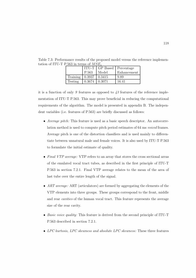
118

Table 7.3: Performance results of the proposed model versus the reference implemen-tation of ITU-T P.563 in terms of MSEs

ITU-T GP Based PercentageP.563 Model Enhancement

Training 0.3937 0.3415 9.89Testing 0.3674 0.3071 16.41

it is a function of only 9 features as opposed to 43 features of the reference imple-

mentation of ITU-T P.563. This may prove beneficial in reducing the computational

requirements of the algorithm. The model is presented in appendix B. The indepen-

dent variables (i.e. features of P.563) are briefly discussed as follows:

• Average pitch: This feature is used as a basic speech descriptor. An autocorre-

lation method is used to compute pitch period estimates of 64 ms voiced frames.

Average pitch is one of the distortion classifiers and is used mainly to di!eren-

tiate between unnatural male and female voices. It is also used by ITU-T P.563

to formulate the initial estimate of quality.

• Final VTP average: VTP refers to an array that stores the cross sectional areas

of the emulated vocal tract tubes, as described in the first principle of ITU-T

P.563 in section 7.2.1. Final VTP average relates to the mean of the area of

last tube over the entire length of the signal.

• ART average: ART (articulators) are formed by aggregating the elements of the

VTP elements into three groups. These groups correspond to the front, middle

and rear cavities of the human vocal tract. This feature represents the average

size of the rear cavity.

• Basic voice quality: This feature is derived from the second principle of ITU-T

P.563 described in section 7.2.1.

• LPC kurtosis, LPC skewness and absolute LPC skewness: These three features

119

represent statistics relevant to the 21 (LPC) linear predictive coe!cients of the

speech signal. The statistics are computed for the LPCs of each frame and

aggregated over all frames of the signal. Skewness and kurtosis are the 3rd and

4th moments about the mean and are considered to give meaningful insights

into the spectral characteristics of the signal.

• Spectral clarity: This feature is computed for voiced sections of the speech signal

to be analyzed. It corresponds to the di!erence between the values of harmonics

of pitch and the non-harmonic spectral components in the gaps between the

harmonics. First five harmonics of the pitch are used. FFT is used for spectral

estimation.

• Estimated segmental SNR: This feature is used to detect the presence of signal

correlated noise.

7.4 Conclusion

In this chapter we have proposed a novel method to derive superior signal-based

non-intrusive speech quality estimation models. ITU-T P.563 algorithm was used for

feature extraction in this research. Three GP experiments were conducted to find a

viable model. One of the experiments was based solely on the use of GP for model

development, whereas in the subsequent experiments a GA was employed to tune

the leaf-coe"cients of the GP trees. The latter two experiments represent hybrid

optimization approaches. The outcome of the research is a new model for deriving

a speech quality estimation model that outperforms the reference implementation

of ITU-T P.563. The derived model is a function of only 9 features whereas the

reference implementation of P.563 uses 43 features. This may potentially lead to a

computationally more e"cient algorithm. Although, the P.563 algorithm has been

120

used in this research for feature extraction, our approach is more general and can be

used in conjunction with other speech processing algorithms or auditory models.

Chapter 8

Conclusions and Future Work

8.1 Conclusions

The aim of this thesis was to derive e!ective non-intrusive speech quality estimation

models. E!ectiveness was desired in two senses. Firstly, it was sought to derive models

with better prediction accuracy as compared with contemporary models. Secondly, it

was expected that the derived models have better computational e"ciency. To achieve

these objectives genetic programming based symbolic regression has been employed.

Equal emphasis has been paid on deriving parametric and signal-based models. To

these ends, disparate models are presented in chapters 5, 6 and 7 that solve di!erent

problems.

Chapter 5 presents parametric models to estimate speech quality of VoIP in a

narrowband (NB) context. A number of modern NB codecs were employed in this

research. ITU-T P.862 [ITU-T, 2001b] (the PESQ algorithm) was used as a reference

model. The chapter also performs parameter significance analysis by examining the

composition of genomes of the best individuals of evolutionary runs. A descriptive

comparison of the derived models with contemporary models is performed where

121

122

strengths of the proposed models are highlighted.

Chapter 6 takes a step further by deriving e!ective equipment factors for ITU-T

G.107 [ITU-T, 2005a] (the E-Model) in a mixed narrowband/wideband (NB/WB)

context where packet loss and codec related impairments due to NB and WB codecs

may be present. A number of modern NB and WB codecs recommended by ITU-T

were chosen. The derived impairment factors outperform the E-Model for equipment

impairment factors in terms of prediction accuracy. Apart from deriving equipment

impairment factors using GP, an additional advantage of the research was that it used

WB-PESQ [ITU-T, 2005f] for obtaining reference/target values for training. The

methodology presented is, however, generic, and may replace WB-PESQ with any

instrumental model. The advantage of using instrumental models such as WB-PESQ

is that the results can be derived quickly.

The focus of chapter 7 was on derivation of signal-based models for speech quality

estimation. To this aim ITU-T P.563 [ITU-T, 2005d] was used as a feature extraction

algorithm. A hybrid optimization approach was employed in which GP was used to

find an appropriate structure of the target model, where a genetic algorithm (GA)

was employed to tune the leaf coe"cients of GP trees during evolution. Various

experiments were performed and the aim was to derive a better model for mapping

the features of ITU-T P.563 on to speech quality. Thus, a nonlinear model was found

that outperformed the linear mapping function of the reference implementation of

ITU-T P.563. The resulting model also had a reduced dimensionality as it was a

function only of 9 features of the ITU-T P.563 algorithm as opposed to the 43 features

of the reference implementation of the algorithm. This may be useful in enhancing

the computational e"ciency of the algorithm.

The results of this thesis further consolidate the notion of GP being a strong ma-

chine learning algorithm. Of special interest is the algorithm’s ability to solve a user

defined problem with minimal user intervention. As compared to other approaches

123

where the practitioner has to deal with worries of manual curve fitting or finding an

appropriate model structure for target data, GP performs these tasks automatically

once provided with the data of the problem domain. In addition it also lends it-

self to easy integration with other numerical coe"cient optimization algorithms. An

application of this has also been demonstrated in chapter 7.

8.2 Future Work

A plethora of future goals and research problems may be defined in the light of this

thesis. These are discussed as follows:

1. It must be emphasized that the focus of this research was to derive quality

estimation models for listening only scenarios. A future objective would be to

derive a model for conversational quality estimation of a call. Conversational

quality su!ers due to increase in the end-to-end delay. A next objective may

be to estimate the combined e!ect of VoIP tra"c parameters including the

end-to-end delay on call quality.

2. In chapter 7 a signal-based model was proposed for speech quality estimation.

An immediate future objective could be to test the model on a wider variety of

network distortion conditions. An additional future objective is to benchmark

the computational performance of the proposed model.

3. Current signal-based non-intrusive models are designed for NB telephony. A

major trend in non-intrusive estimation of speech quality is towards WB signals.

Chapter 6 was dedicated to derivation of equipment impairment factors for E-

Model in a mixed NB/WB context. As a followup of that a future research goal

may be to develop a signal-based model for a mixed NB/WB context.

124

4. Development of a hybrid non-intrusive model that is a function of cogent trans-

port layer metrics as well as of significant features of the speech signal under

test. This is aimed at achieving a higher prediction accuracy by circumventing

the weaknesses of both types of models.

Bibliography

[A. D. Clark, 1998] A. D. Clark (1998). Description of The VQMON Algorithm. In-

ternational Telecommunications Union, Geneva, Switzerland. ITU-T Delayed Con-

tribution COM12-D105.

[Banzhaf et al., 1998] Banzhaf, W., Nordin, P., Keller, R. E., and Francone, F. D.

(1998). Genetic Programming – An Introduction; On the Automatic Evolution of

Computer Programs and its Applications. Morgan Kaufmann, dpunkt.verlag.

[Barriac et al., 2004] Barriac, V., Sout, J. Y., and Lockwood, C. (2004). Discussion

on unified objective methodologies for the comparison of voice quality of narrow-

band and wideband scenarios. In In. Proc. Workshop on Wideband Speech Quality

in Terminals and Networks: Assessment and Prediction.

[Beerends, 1995] Beerends, J. G. (1995). Measuring the quality of speech and music

codecs: An integrated psychoacoustic approach. In: Preprints of the 98th Conven-

tion of the Audio Engineering Society, (3945).

[Bishop, 1995] Bishop, C. M. (1995). Neural Networks for Pattern Recognition. Ox-

ford University Press, Inc., New York, NY, USA.

[Blauert, 1997] Blauert, J. (1997). Spatial Hearing: The Psychophysics of Human

Sound Localization. MIT Press USA, Cambridge, MA.

125

126

[Bolot, 1993] Bolot, J.-C. (1993). Characterizing end-to-end packet delay and loss in

the internet.

[Braden et al., 1997] Braden, R., Zhang, L., Berson, S., Herzog, S., and Jamin, S.

(1997). Resource ReSerVation Protocol (RSVP) – Version 1 Functional Specifica-

tion. RFC 2205 (Proposed Standard). Updated by RFCs 2750, 3936, 4495.

[Casner and Jacobson, 1999] Casner, S. and Jacobson, V. (1999). Compressing

IP/UDP/RTP Headers for Low-Speed Serial Links. RFC 2508 (Proposed Stan-

dard).

[Chu, 2003] Chu, W. C. (2003). Speech Coding Algorithms: Foundation and Evolution

of Standardized Codecs. John Wiley and Sons Inc, Cambridge, MA, USA.

[Clark, 2001] Clark, A. D. (2001). Modeling the e!ects of burst packet loss and

recency on subjective voice quality. In 2nd IP-Telephony Workshop, Columbia

University, New York.

[Cole and Rosenbluth, 2001] Cole, R. G. and Rosenbluth, J. H. (2001). Voice over ip

performance monitoring. SIGCOMM Comput. Commun. Rev., 31(2):9–24.

[Conway, 2002] Conway, A. E. (2002). A passive method for monitoring voice-over-ip

call quality with itu-t objective speech quality measurement methods. In Com-

munications, 2002. ICC 2002. IEEE International Conference on, volume 4, pages

2583–2586 vol.4.

[Conway, 2004] Conway, A. E. (2004). Output-based method of applying pesq to

measure the perceptual quality of framed speech signals. In IEEE Conference on

Wireless Communications and Networking, volume 4, pages 2521–2526.

[Davidson et al., 2006] Davidson, J., Peters, J., Bhatia, M., Kalidindi, S., and

Mukherjee, S. (2006). Voice over IP Fundamentals (2nd Edition) (Fundamentals).

Cisco Press.

127

[Davis, 1989] Davis, L. (1989). Adapting operator probabilities in genetic algorithms.

In Proceedings of the Third International Conference on Genetic Algorithms, San

Mateo, CA.

[Diethorn, 1997] Diethorn, E. J. (7-10 Sep 1997). A low-complexity, background-noise

reduction preprocessor for speech encoder. Speech Coding For Telecommunications

Proceeding, 1997, 1997 IEEE Workshop on, pages 45–46.

[Esparcia-Alcazar and Sharman, 1997] Esparcia-Alcazar, A. I. and Sharman, K.

(1997). Learning schemes for genetic programming. In Late Breaking Papers at the

Genetic Programming 97 Conference, pages 57–65, Stanford University, USA.

[ETSI, 2000] ETSI (2000). Universal Mobile Telecommunications Systems (UMTS);

Mandatory Speech Codec Speech Processing Functions AMR Speech Codec; General

Description. European Telecommunications Standards Institute.

[Everitt and Hand, 1981] Everitt, B. S. and Hand, D. J. (1981). Finite mixture dis-

tributions. Monographs on Applied Probability and Statistics, London: Chapman

and Hall, 1981.

[Falk and Chan, 2006] Falk, T. H. and Chan, W.-Y. (2006). Single-ended speech

quality measurement using machine learning methods. IEEE Transactions on Au-

dio, Speech and Language Processing, 14(6):1935–1947.

[Friedman, 1991] Friedman, J. H. (1991). Multivariate adaptive regression splines.

The Annals of Statistics, 19(1):1–67.

[Friedman et al., 2003] Friedman, T., Caceres, R., and Clark, A. (2003). RTP Control

Protocol Extended Reports (RTCP XR). RFC 3611 (Proposed Standard).

[Fujimoto et al., 2002] Fujimoto, K., Ata, S., and Murata, M. (17-21 Nov. 2002).

Adaptive playout bu!er algorithm for enhancing perceived quality of streaming

128

applications. In Global Telecommunications Conference, 2002. GLOBECOM ’02.

IEEE, volume 3, pages 2451–2457 vol.3.

[Gagne and Parizeau, 2006] Gagne, C. and Parizeau, M. (2006). Open BEAGLE A

C++ framework for your favorite evolutionary algorithm. SIGEvolution, 1(1):12–

15.

[Gold and Morgan, 1999] Gold, B. and Morgan, N. (1999). Speech and Audio Signal

Processing: Processing and Perception of Speech and Music. Wiley, New York, NY,

USA.

[Goldberg, 1989] Goldberg, D. E. (1989). Genetic Algorithms in Search, Optimization

and Machine Learning. Addison-Wesley Longman Publishing Co., Inc., Boston,

MA, USA.

[Goldberg and Deb, 1990] Goldberg, D. E. and Deb, K. (1990). A comparative anal-

ysis of selection schemes used in genetic algorithms. In FOGA, pages 69–93.

[Grancharov et al., 2006] Grancharov, V., Zhao, D. Y., Lindblom, J., and Kleijn,

W. B. (2006). Low-complexity, nonintrusive speech quality assessment. IEEE

Transactions on Audio, Speech and Language Processing, 14(6):1948–1956.

[Gray et al., 2000] Gray, P., Hollier, M. P., and Massara, R. E. (2000). Non-intrusive

speech-quality assessment using vocal-tract models. In IEE Proceedings of Vision,

Image and Signal Processing, volume 147.

[Gustafson et al., 2005] Gustafson, S., Burke, E. K., and Krasnogor, N. (2005). On

improving genetic programming for symbolic regression. In et. al., D. C., editor,

Proceedings of the 2005 IEEE Congress on Evolutionary Computation, volume 1,

pages 912–919, Edinburgh, UK. IEEE Press.

129

[Hammer et al., 2003] Hammer, F., Reichl, P., Nordstrom, T., and Kubin, G. (2003).

Corrupted speech data considered useful. In Proc. First ISCA International Tu-

torial and Research Workshop on Auditory Quality of Systems, Mont-Cenis, Ger-

many.

[Hermansky, 1990] Hermansky, H. (1990). Perceptual Linear Predictive (PLP) Anal-

ysis of Speech. Journal of Acoustical Society of America, 87(4):1738–1752.

[Hoene et al., 2004] Hoene, C., Karl, H., and Wolisz, A. (2004). A perceptual quality

model for adaptive voip applications. In In Proc. of International Symposium on

Performance Evaluation of Computer and Telecommunication Systems (SPECTS),

volume 4, pages 2573–2577, San Jose, California, USA.

[Hoene et al., 2005] Hoene, C., Karl, H., and Wolisz, A. (2005). A perceptual quality

model intended for adaptive VoIP applications. International Journal of Commu-

nications Systems, 99(7):1–20.

[Howard and D’Angelo, 1995] Howard, L. M. and D’Angelo, D. J. (1995). The GA–P:

A genetic algorithm and genetic programming hybrid. IEEE Expert, 10(3):11–15.

[ITU-T, 1988a] ITU-T (1988a). 7 kHz Audio coding within 64 kbit/s. International

Telecommunications Union, Geneva, Switzerland. ITU-T Recommendation G.722.

[ITU-T, 1988b] ITU-T (1988b). Pulse Code Modulation (PCM) of voice frequencies.

International Telecommunications Union, Geneva, Switzerland. ITU-T Recommen-

dation G.711.

[ITU-T, 1990a] ITU-T (1990a). 40, 32, 24, 16 kbit/s Adaptive Di"erential Pulse

Code Modulation (ADPCM). International Telecommunications Union, Geneva,

Switzerland. ITU-T Recommendation G.726.

130

[ITU-T, 1990b] ITU-T (1990b). 5-, 4-, 3- AND 2-BITS SAMPLE EMBEDDED

ADAPTIVE DIFFERENTIAL PULSE CODE MODULATION (ADPCM). Inter-

national Telecommunications Union, Geneva, Switzerland. ITU-T Recommenda-

tion G.727.

[ITU-T, 1996a] ITU-T (1996a). Coding of Speech at 8 kbit/s using conjugate-structure

algebraic-code-excited linear-prediction (CS-ACELP). International Telecommuni-

cations Union, Geneva, Switzerland. ITU-T Recommendation G.729.

[ITU-T, 1996b] ITU-T (1996b). Dual rate speech coder for multimedia communica-

tion transmitting at 5.3 and 6.3 kbit/s. International Telecommunications Union,

Geneva, Switzerland. ITU-T Recommendation G.723.1.

[ITU-T, 1996c] ITU-T (1996c). Methods for subjective determination of transmission

quality. International Telecommunications Union, Geneva, Switzerland. ITU-T

Recommendation P.800.

[ITU-T, 1996d] ITU-T (1996d). Subjective performance assessment of telephone-band

and wideband digital codecs. International Telecommunications Union, Geneva,

Switzerland. ITU-T Recommendation P.830.

[ITU-T, 1998a] ITU-T (1998a). coded-speech database. International Telecommuni-

cations Union, Geneva, Switzerland. ITU-T P.Supplement 23.

[ITU-T, 1998b] ITU-T (1998b). Objective quality measurement of telephone-band

(300-3400 Hz) speech codecs. International Telecommunications Union, Geneva,


[ITU-T, 1998c] ITU-T (1998c). Subject Performance Evaluation of Network Echo

Cancellers. International Telecommunications Union, Geneva, Switzerland. ITU-T


131

[ITU-T, 1998d] ITU-T (1998d). Terms and Definitions Related to Quality of Service

and Network Performance Including Dependability. International Telecommunica-

tions Union, Geneva, Switzerland. ITU-T Recommendation E.800.

[ITU-T, 2000] ITU-T (2000). Subject Performance Evaluation of Hands-Free Ter-

minals. International Telecommunications Union, Geneva, Switzerland. ITU-T


[ITU-T, 2001a] ITU-T (2001a). Methodology for derivation of equipment impair-

ment factors from subjective listening-only tests. International Telecommunications

Union, Geneva, Switzerland. ITU-T Recommendation P.833.

[ITU-T, 2001b] ITU-T (2001b). Perceptual evaluation of speech quality (PESQ), an

objective method for end-to-end speech quality assessment of narrowband telephone

networks and speech codecs. International Telecommunications Union, Geneva,


[ITU-T, 2002] ITU-T (2002). Methodology for the derivation of equipment impair-

ment factors from instrumental models. International Telecommunications Union,

Geneva, Switzerland. ITU-T Recommendation P.834.

[ITU-T, 2003a] ITU-T (2003a). Mapping function for transforming P.862 raw result

scores to MOS-LQO. International Telecommunications Union, Geneva, Switzer-

land. ITU-T Recommendation P.862.1.

[ITU-T, 2003b] ITU-T (2003b). Mean opinion score (MOS) terminology. Interna-

tional Telecommunications Union, Geneva, Switzerland. ITU-T Recommendation

P.800.1.

[ITU-T, 2003c] ITU-T (2003c). One-way transmission time. International Telecom-

munications Union, Geneva, Switzerland. ITU-T Recommendation G.114.

132

[ITU-T, 2003d] ITU-T (2003d). Wideband coding of speech at around 16 kbit/s us-

ing Adaptive Multi-Rate Wideband (AMR-WB). International Telecommunications

Union, Geneva, Switzerland. ITU-T Recommendation G.722.2.

[ITU-T, 2004] ITU-T (2004). Continuous Evaluation of Time-Varying Speech Qual-

ity. International Telecommunications Union, Geneva, Switzerland. ITU-T Rec-

ommendation P.880.

[ITU-T, 2005a] ITU-T (2005a). The E-Model, a computational model for use in trans-

mission planning. International Telecommunications Union, Geneva, Switzerland.

ITU-T Recommendation G.107.

[ITU-T, 2005b] ITU-T (2005b). Low-complexity coding at 24 and 32 kbit/s for hands-

free operation in systems with low frame loss. International Telecommunications

Union, Geneva, Switzerland. ITU-T Recommendation G.722.1.

[ITU-T, 2005c] ITU-T (2005c). Network model for evaluating multimedia transmis-

sion performance over internet protocol. International Telecommunications Union,

Geneva, Switzerland. ITU-T Recommendation G.1050.

[ITU-T, 2005d] ITU-T (2005d). Single-ended method for objective speech quality as-

sessment in narrow-band telephony applications. International Telecommunications

Union, Geneva, Switzerland. ITU-T Recommendation P.563.

[ITU-T, 2005e] ITU-T (2005e). Software tools for speech and audio coding standard-

ization. International Telecommunications Union, Geneva, Switzerland. ITU-T

Recommendation G.191.

[ITU-T, 2005f] ITU-T (2005f). Wideband extension to Recommendation P.862 for

the assessment of wideband telephone networks and speech codecs. Interna-

tional Telecommunications Union, Geneva, Switzerland. ITU-T Recommendation

P.862.2.

133

[ITU-T, 2006a] ITU-T (2006a). G.729 based Embedded Variable bit-rate coder: An 8-

32 kbit/s scalable wideband coder bitstream interoperable with G.729. International

Telecommunications Union, Geneva, Switzerland. ITU-T Recommendation G.729.

[ITU-T, 2006b] ITU-T (2006b). New Appendix IV – Provisional planning values for

the wideband equipment impairment factor Ie,wb. International Telecommunica-

tions Union, Geneva, Switzerland. ITU-T Recommendation G.113.

[Janssen et al., 2002] Janssen, J., Vleeschauwer, D. D., Buchli, M., and Petit, G. H.

(2002). Assessing voice quality in packet-based telephony. IEEE Internet Comput-

ing, 6(3):48–56.

[Jekosch, 2005] Jekosch, U. (2005). Voice and Speech Quality Perception Assessment

and Evaluation Signals and Communication Technology. Springer D–Berlin.

[Jiang and Schulzrinne, 2000] Jiang, W. and Schulzrinne, H. (2000). Modeling of

packet loss and delay and their e!ect on real-time multimedia service quality. In

In Proc. NOSSDAV.

[Jiang and Schulzrinne, 2002] Jiang, W. and Schulzrinne, H. (2002). Perceived qual-

ity of packet audio under bursty losses. In Annual Joint Conference of the IEEE

Computer and Communications Societies (INFOCOM), York, UK.

[Jin and Kubichek, 1995] Jin, C. and Kubichek, R. (1995). Output-based objective

speech quality using vector quantization techniques. In IEEE Conference on Signals

Systems and Computers, volume 2, pages 1291–1294.

[Jin and Kubichek, 1996] Jin, C. and Kubichek, R. (1996). Vector quantization tech-

niques for output-based objective speech quality. In IEEE International Conference

on Acoustic, Speech and Signal Processing (ICASSP), volume 1, pages 1291–1294.

[Keijzer, 2003] Keijzer, M. (2003). Improving symbolic regression with interval arith-

metic and linear scaling. In Ryan, C., Soule, T., Keijzer, M., Tsang, E., Poli, R.,

134

and Costa, E., editors, Genetic Programming, Proceedings of EuroGP’2003, volume

2610 of LNCS, pages 70–82, Essex. Springer-Verlag.

[Keijzer, 2004] Keijzer, M. (2004). Scaled symbolic regression. Genetic Programming

and Evolvable Machines, 5(3):259–269.

[Keith and Martin, 1994] Keith, M. J. and Martin, M. C. (1994). Genetic program-

ming in C++: Implementation issues. In Kinnear, Jr., K. E., editor, Advances in

Genetic Programming, chapter 13, pages 285–310. MIT Press.

[Kim, 2005] Kim, D.-S. (2005). Anique: An auditory model for single-ended speech

quality estimation. IEEE Transactions on Speech and Audio Processing, 13(5):821–

831.

[Kim, 2004] Kim, D.-S. (Oct. 2004). A cue for objective speech quality estimation in

temporal envelope representations. Signal Processing Letters, IEEE, 11(10):849–

852.

[Kirkpatrick et al., 1983] Kirkpatrick, S., Gelatt, C. D., and Vecchi, M. P. (1983).

Optimization by simulated annealing. Science, Number 4598, 13 May 1983, 220,

4598:671–680.

[Kohonen, 1990] Kohonen, T. (Sep 1990). The self-organizing map. Proceedings of

the IEEE, 78(9):1464–1480.

[Koza, 1992] Koza, J. R. (1992). Genetic Programming: On the Programming of

Computers by Means of Natural Selection. MIT Press, Cambridge, MA, USA.

[Langdon and Buxton, 2004] Langdon, W. B. and Buxton, B. F. (2004). Genetic pro-

gramming for mining DNA chip data from cancer patients. Genetic Programming

and Evolvable Machines, 5(3):251–257.

135

[Li and Kubichek, 2003] Li, W. and Kubichek, R. (2003). Output-based objective

speech quality measurement using continuous Hidden Markov Models. In Sev-

enth International Symposium on Signal Processing and Its Applications, 2003,

volume 1, pages 1–4.

[Liang and Kubichek, 1994] Liang, J. and Kubichek, R. F. (1994). Output-based ob-

jective speech quality. In 44th IEEE Conference on Vehicular Technology, volume 3,

pages 1719–1723.

[Luke and Panait, 2002] Luke, S. and Panait, L. (2002). Lexicographic parsimony

pressure. In et. al., W. B. L., editor, GECCO 2002: Proceedings of the Genetic

and Evolutionary Computation Conference, pages 829–836, New York.

[Makhoul, 1975] Makhoul, J. (1975). Linear prediction: A tutorial review. Proceed-

ings of the IEEE, 63(4):561–580.

[Minoli and Minoli, 1998] Minoli, D. and Minoli, E. (1998). Delivering voice over IP

networks. John Wiley & Sons, Inc., New York, NY, USA.

[Mitchell, 1997] Mitchell, T. (1997). Machine Learning. McGraw Hill, New York.

[Mohamed et al., 2001] Mohamed, S., Cervantes-Perez, F., and Afifi, H. (2001). In-

tegrating networks measurements and speech quality subjective scores for control

purposes. In Annual Joint Conference of the IEEE Computer and Communications

Societies (INFOCOM), pages 641–649.

[Mohamed et al., 2004] Mohamed, S., Rubino, G., and Varela, M. (2004). A method

for quantitative evaluation of audio quality over packet networks and its comparison

with existing techniques. In Measurement of Speech and Audio Quality in Networks

(MESAQIN).

[Moller, 2000] Moller, S. (2000). Assessment and Prediction of Speech Quality in

Telecommunications. Springer D–Berlin.

136

[Moller et al., 2006] Moller, S., Raake, A., Kitawaki, N., Takahashi, A., and Wal-

termann, M. (2006). Impairment factor framework for wide-band speech codecs.

IEEE Transactions on Audio, Speech and Language Processing, 16(6):1969–1976.

[Moon et al., 1998] Moon, S. B., Kurose, J., and Towsley, D. (1998). Packet audio

playout delay adjustment: Performance bounds and algorithms. Multimedia Syst.,

6(1):17–28.

[Morioka et al., 2004] Morioka, C., Kurashima, A., and Takahashi, A. (2004). Pro-

posal on objective speech quality assessment for wideband telephony. In IEEE

International Conference on Acoustic, Speech and Signal Processing (ICASSP).

[Mugambi et al., 2004] Mugambi, E. M., Hunter, A., Oatley, G., and Kennedy, L.

(2004). Polynomial-fuzzy decision tree structures for classifying medical data.

Knowledge-Based Systems, 17(2-4):81–87.

[Narbutt and Davis, 2005] Narbutt, M. and Davis, M. (2005). Assessing the quality of

VoIP transmission a!ected by playout bu!er scheme. In Measurement of Speech and

Audio Quality in Networks (MESAQIN), Czech Technical University, CZ-Prague.

[Neto et al., 1999] Neto, S. F. C., Corcoran, F. L., and Karahisar, A. (1999). Perfor-

mance assessment of tandem connection of enhanced cellular coders. In ICASSP

’99: Proceedings of the Acoustics, Speech, and Signal Processing, 1999. on 1999

IEEE International Conference, pages 177–180, Washington, DC, USA. IEEE

Computer Society.

[Nichols et al., 1998] Nichols, K., Blake, S., Baker, F., and Black, D. (1998). Defini-

tion of the Di!erentiated Services Field (DS Field) in the IPv4 and IPv6 Headers.

RFC 2474 (Proposed Standard). Updated by RFCs 3168, 3260.

[O’Neill and Ryan, 2001] O’Neill, M. and Ryan, C. (2001). Grammatical evolution.

IEEE Transactions on Evolutionary Computation, 5(4):349–358.

137

[Pennock, 2002] Pennock, S. (2002). Accuracy of the perceptual evaluation of speech

quality (PESQ) algorithm. In Measurement of Speech and Audio Quality in Net-

works (MESAQIN).

[Perkins et al., 1998] Perkins, C., Hodson, O., and Hardman, V. (1998). A survey of

packet loss recovery techniques for streaming audio. IEEE Network, 12:40–48.

[Perkins et al., 1997] Perkins, C., Kouvelas, I., Hodson, O., Hardman, V., Handley,

M., Bolot, J., Vega-Garcia, A., and Fosse-Parisis, S. (1997). RTP Payload for

Redundant Audio Data. RFC 2198 (Proposed Standard).

[Picovici and Mahdi, 2004] Picovici, D. and Mahdi, A. E. (2004). New output-based

perceptual measure for predicting subjective quality of speech. In IEEE Interna-

tional Conference on Acoustic, Speech and Signal Processing (ICASSP), volume 5,

pages 17–21.

[Quackenbush et al., 1988] Quackenbush, S. R., Barnwell, T. P., and Clements, M. A.

(1988). Objective Measures of Speech Quality. Prentice-Hall, Englewood Cli!s, NJ.

[Raake, 2006] Raake, A. (2006). Speech Quality of VoIP Assessment and Prediction.

John Wiley and Sons Inc.

[Rabiner, 1989] Rabiner, L. (Feb 1989). A tutorial on hidden markov models and

selected applications in speech recognition. Proceedings of the IEEE, 77(2):257–

286.

[Raja et al., 2006] Raja, A., Azad, R. M. A., Flanagan, C., Picovici, D., and Ryan,

C. (2006). Non-intrusive quality evaluation of voip using genetic programming.

In First International Conference on Bio Inspired Models of Network, Information

and Computer Systems, volume 4, pages 2573–2577.

[Raja et al., 2007] Raja, A., Azad, R. M. A., Flanagan, C., and Ryan, C. (2007).

Real-time, non-intrusive evaluation of VoIP. In Ebner, M., O’Neill, M., Ekart,

138

A., Vanneschi, L., and Esparcia-Alcazar, A. I., editors, Proceedings of the 10th

European Conference on Genetic Programming, volume 4445 of Lecture Notes in

Computer Science, pages 217–228, Valencia, Spain. Springer.

[Ramjee et al., 1994] Ramjee, R., Kurose, J. F., Towsley, D. F., and Schulzrinne, H.

(1994). Adaptive playout mechanisms for packetized audio applications in wide-

area networks. In INFOCOM (2), pages 680–688.

[Ramsey, 1970] Ramsey, J. L. (May 1970). Realization of optimum interleavers. In-

formation Theory, IEEE Transactions on, 16(3):338–345.

[Rix et al., 2006] Rix, A. W., Beerends, J. G., Kim, D.-S., Kroon, P., and Ghitza,

O. (Nov. 2006). Objective assessment of speech and audio qualitytechnology and

applications. Audio, Speech, and Language Processing, IEEE Transactions on [see

also Speech and Audio Processing, IEEE Transactions on], 14(6):1890–1901.

[Rix et al., 2002] Rix, A. W., Hollier, M. P., Hekstra, A. P., and Beerends, J. G.

(2002). Perceptual evaluation of speech quality (pesq) the new itu standard for

end-to-end speech quality assessment part i–time-delay compensation. Journal of

Audio Engineering Society (AES), 50(10):755–764.

[Rix, 2000] Rix, A.W.; Hollier, M. (2000). The perceptual analysis measurement sys-

tem for robust end-to-end speech quality assessment. Acoustics, Speech, and Signal

Processing, 2000. ICASSP ’00. Proceedings. 2000 IEEE International Conference

on, 3:1515–1518 vol.3.

[Rosen et al., 2001] Rosen, E., Viswanathan, A., and Callon, R. (2001). Multiproto-

col Label Switching Architecture. RFC 3031 (Proposed Standard).

[Rosenberg et al., 2000] Rosenberg, J., Qiu, L., and Schulzrinne, H. (2000). Integrat-

ing packet FEC into adaptive voice playout bu!er algorithms on the internet. In

INFOCOM (3), pages 1705–1714.

139

[Rosenberg and Schulzrinne, 1999] Rosenberg, J. and Schulzrinne, H. (1999). An

RTP Payload Format for Generic Forward Error Correction. RFC 2733 (Proposed

Standard).

[Rosenberg, 2001] Rosenberg, J. D. (2001). G.729 error recovery for internet tele-

phony. Technical report, Columbia University Computer Science Technical Report

CUCS-016-01.

[Sanneck and Carle, 2000] Sanneck, H. and Carle, G. (2000). A framework model for

packet loss metrics based on loss runlengths. In SPIE/ACM SIGMM Multimedia

Computing and Networking Conference.

[Schulzrinne et al., 2003] Schulzrinne, H., Casner, S., Frederick, R., and Jacobson,

V. (2003). RTP: A Transport Protocol for Real-Time Applications. RFC 3550

(Standard).

[Sharman et al., 1995] Sharman, K. C., Esparcia-Alcazar, A. I., and Li, Y. (1995).

Evolving digital signal processing algorithms by genetic programming. Technical

Report CSC-95012, Faculty of Engineering, Glasgow G12 8QQ, Scotland.

[Sun and Ifeachor, 2002a] Sun, L. and Ifeachor, E. C. (2002a). perceived speech qual-

ity prediction for voice over ip-based networks. In IEEE International Conference

on Communications (ICC), volume 4, pages 2573–2577.

[Sun and Ifeachor, 2002b] Sun, L. and Ifeachor, E. C. (2002b). Subjective and objec-

tive speech quality evaluation under bursty losses. In Measurement of Speech and

Audio Quality in Networks (MESAQIN).

[Sun and Ifeachor, 2006] Sun, L. and Ifeachor, E. C. (2006). Voice quality prediction

models and their application in VoIP networks. IEEE Transactions on Multimedia,

8(4):809– 820.

140

[Tarraf and Meyers, 1999] Tarraf, A. and Meyers, M. (1999). Neural network-based

voice quality measurement technique. In IEEE international symposium on Com-

puters and Communications, pages 375–381.

[Thorpe and Yang, 1996] Thorpe, L. and Yang, W. (1996). Performance of current

perceptual objective speech quality measures. In IEEE International Speech Cod-

ing, volume 1, pages 144–146.

[Topchy and Punch, 2001] Topchy, A. and Punch, W. F. (2001). Faster genetic pro-

gramming based on local gradient search of numeric leaf values. In Spector, L.,

Goodman, E. D., Wu, A., Langdon, W. B., Voigt, H.-M., Gen, M., Sen, S., Dorigo,

M., Pezeshk, S., Garzon, M. H., and Burke, E., editors, Proceedings of the Genetic

and Evolutionary Computation Conference (GECCO-2001), pages 155–162, San

Francisco, California, USA. Morgan Kaufmann.

[Voran, 1999a] Voran, S. (1999a). Objective estimation of perceived speech quality.

I. development of the measuring normalizing block technique. IEEE Transactions

on Speech and Audio Processing, 7(4):371–382.

[Voran, 1999b] Voran, S. (1999b). Objective estimation of perceived speech quality.

I. development of the measuring normalizing block technique. IEEE Transactions

on Speech and Audio Processing, 7(4):383–390.

[Walpole et al., 1998] Walpole, R. E., Myers, R. H., and Myers, S. L. (1998). Proba-

bility and Statistics for Engineers and Scientists. prentice Hall International, Inc,

New Jersey.

[Yajnik et al., 1999] Yajnik, M., Moon, S. B., Kurose, J. F., and Towsley, D. F.

(1999). Measurement and modeling of the temporal dependence in packet loss. In

INFOCOM (1), pages 345–352.

141

[Zhong et al., 2005] Zhong, J., Hu, X., Zhang, J., and Gu, M. (2005). Comparison

of performance between di!erent selection strategies on simple genetic algorithms.

In CIMCA ’05: Proceedings of the International Conference on Computational

Intelligence for Modelling, Control and Automation and International Conference

on Intelligent Agents, Web Technologies and Internet Commerce Vol-2 (CIMCA-

IAWTIC’06), pages 1115–1121, Washington, DC, USA. IEEE Computer Society.

[Zopf, 2002] Zopf, R. (2002). Real-time Transport Protocol (RTP) Payload for Com-

fort Noise (CN). RFC 3389 (Proposed Standard).

[Zwicker, 1961] Zwicker, E. (1961). Subdivision of the audible frequency range into

critical bands (frequenzgruppen). The Journal of the Acoustical Society of America,

33(2):248–248.

[Zwillinger, 2003] Zwillinger, D. (2003). CRC Standard Mathematical Tables and For-

mulae. Boca Raton, FL: CRC Press, 31st edition.

Appendix A

Transformation Between MOS andR

This appendix presents the equations to transform MOS to R and vice versa. R can

be converted to MOS using equation (A.0.1).

MOS =

,

-

-

-

-

-

.

-

-

-

-

-

/

1 for R $ 0

1 + 0.035R + R(R ! 60)

&(100 ! R)7 & 106, for 0 < R < 100

4.5 for R % 100

(A.0.1)

Similarly, Hoene et al. in [Hoene et al., 2004] proposed an inversion of equation

(A.0.1) which is now a part of the E-Model (see Appendix I in [ITU-T, 2005a]). In

the range 6.5$ R$ 100, R can be calculated from MOS using the formula:

R =20

3

$

8 !)

226cos$

h +#

3

&&

(A.0.2)

with:

h =1

3arctan2

$

18566 ! 6750MOS, 15)!903522 + 1113960MOS ! 202500MOS2

&

(A.0.3)

and:

142

143

arctan2(x, y) =

0

arctan'

yx

(

for x % 0

# ! arctan'

y!x

(

for x < 0(A.0.4)

Appendix B

Signal-based Model

This appendix presents the signal-based non-intrusive model resulting from the re-

search presented in chapter 7. The model is presented using tree representation. The

interpretation of the functions and terminals is as follows:

+: Add

-: Subtract

*: Multiplication

/: Division

ln: Natural logarithm

x1: Average pitch

x2: Final VTP average

x3: ART average

x4: Basic voice quality

x5: LPC kurtosis

x6: LPC skewness

x7: Absolute LPC skewness

x8: Spectral clarity

x9: Estimated segmental SNR

144

145

+

+ ln

+

x5

-

+

*

+

x6

x4

ln

x3

ln

*

x7 *

x9 *

* *

x8 x9

x5 *

- *

*

x2

x2

x2

x2

+

x1

x2

x4 - + ln

*

x3

ln

/

*

* x2 x2 x9

*

* x7 x5 x6

x6 *

* -

*

x9 x9

* x2

x8 x9

x8

ln

-0.4414

0.0838

ln

x2 x9

* x2

*

x4

+

*

x9 x8

* x6 -

6 5

-

3

ln

* +

Figure B.1: Signal-based model resulting from the research presented in chapter 7

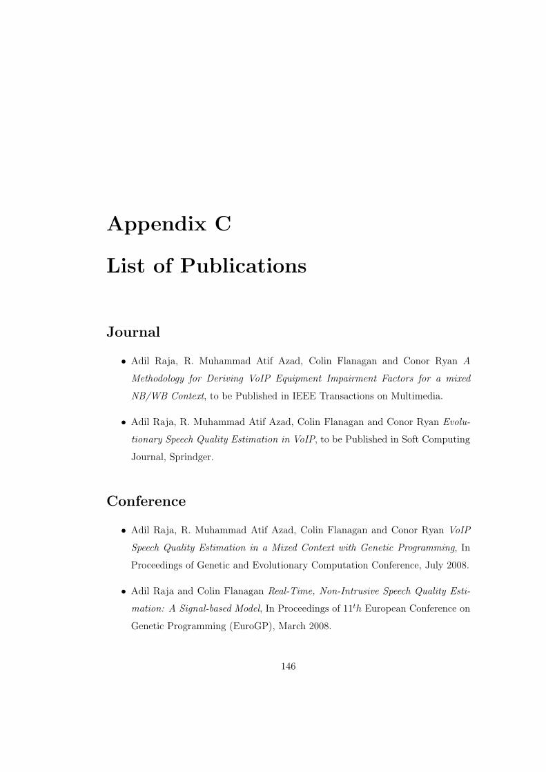
Appendix C

List of Publications

Journal

• Adil Raja, R. Muhammad Atif Azad, Colin Flanagan and Conor Ryan A

Methodology for Deriving VoIP Equipment Impairment Factors for a mixed

NB/WB Context, to be Published in IEEE Transactions on Multimedia.

• Adil Raja, R. Muhammad Atif Azad, Colin Flanagan and Conor Ryan Evolu-

tionary Speech Quality Estimation in VoIP, to be Published in Soft Computing

Journal, Sprindger.

Conference

• Adil Raja, R. Muhammad Atif Azad, Colin Flanagan and Conor Ryan VoIP

Speech Quality Estimation in a Mixed Context with Genetic Programming, In

Proceedings of Genetic and Evolutionary Computation Conference, July 2008.

• Adil Raja and Colin Flanagan Real-Time, Non-Intrusive Speech Quality Esti-

mation: A Signal-based Model, In Proceedings of 11th European Conference on

Genetic Programming (EuroGP), March 2008.

146

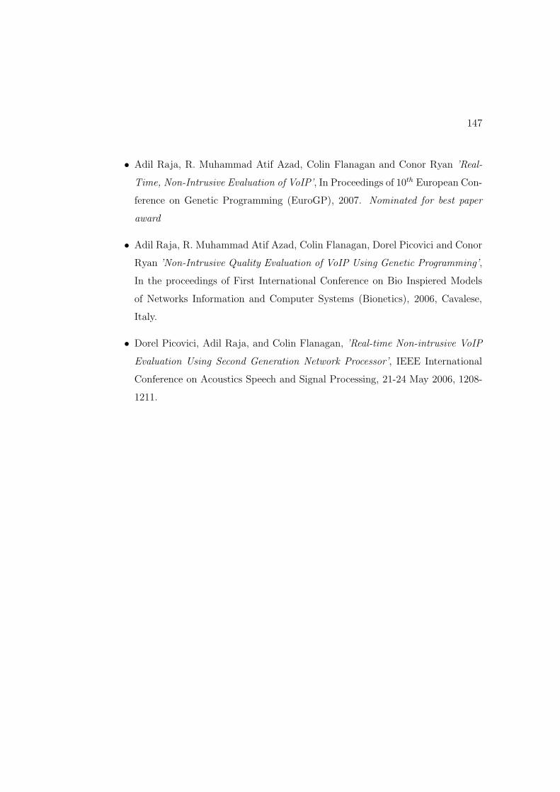
147

• Adil Raja, R. Muhammad Atif Azad, Colin Flanagan and Conor Ryan ’Real-

Time, Non-Intrusive Evaluation of VoIP’, In Proceedings of 10th European Con-

ference on Genetic Programming (EuroGP), 2007. Nominated for best paper

award

• Adil Raja, R. Muhammad Atif Azad, Colin Flanagan, Dorel Picovici and Conor

Ryan ’Non-Intrusive Quality Evaluation of VoIP Using Genetic Programming’,

In the proceedings of First International Conference on Bio Inspiered Models

of Networks Information and Computer Systems (Bionetics), 2006, Cavalese,

Italy.

• Dorel Picovici, Adil Raja, and Colin Flanagan, ’Real-time Non-intrusive VoIP

Evaluation Using Second Generation Network Processor’, IEEE International

Conference on Acoustics Speech and Signal Processing, 21-24 May 2006, 1208-

1211.

REAL-TIME NON-INTRUSIVE SPEECH QUALITY ESTIMATION OF … · 2013-02-21 · real-time non-intrusive...

Documents

Transcript of REAL-TIME NON-INTRUSIVE SPEECH QUALITY ESTIMATION OF … · 2013-02-21 · real-time non-intrusive...