Real-Time Multianalysis–Multimodel Superensemble Forecasts...

DECEMBER 2001 2861K R I S H N A M U R T I E T A L .

q 2001 American Meteorological Society

Real-Time Multianalysis–Multimodel Superensemble Forecasts of Precipitation UsingTRMM and SSM/I Products

T. N. KRISHNAMURTI,* SAJANI SURENDRAN,* D. W. SHIN,* RICARDO J. CORREA-TORRES,*T. S. V. VIJAYA KUMAR,* ERIC WILLIFORD,* CHRIS KUMMEROW,1 ROBERT F. ADLER,#

JOANNE SIMPSON,# RAMESH KAKAR,@ WILLIAM S. OLSON,& AND F. JOSEPH TURK**

*Department of Meteorology, The Florida State University, Tallahassee, Florida1Department of Atmospheric Sciences, Colorado State University, Fort Collins, Colorado

#NASA Goddard Space Flight Center, Greenbelt, Maryland@NASA Headquarters, Washington, D.C.

&Joint Center for Earth Systems Technology, University of Maryland, Baltimore County, Baltimore, Maryland**Marine Meteorology Division, Naval Research Laboratory, Monterey, California

(Manuscript received 17 August 2000, in final form 24 May 2001)

ABSTRACT

This paper addresses real-time precipitation forecasts from a multianalysis–multimodel superensemble. The meth-odology for the construction of the superensemble forecasts follows previous recent publications on this topic. Thisstudy includes forecasts from multimodels of a number of global operational centers. A multianalysis componentbased on the Florida State University (FSU) global spectral model that utilizes TRMM and SSM/I datasets and anumber of rain-rate algorithms is also included. The difference in the analysis arises from the use of these rain rateswithin physical initialization that produces distinct differences among these components in the divergence, heating,moisture, and rain-rate descriptions. A total of 11 models, of which 5 represent global operational models and 6represent multianalysis forecasts from the FSU model initialized by different rain-rate algorithms, are included in themultianalysis–multimodel system studied here. In this paper, ‘‘multimodel’’ refers to different models whose forecastsare being assimilated for the construction of the superensemble. ‘‘Multianalysis’’ refers to different initial analysiscontributing to forecasts from the same model. The term superensemble is being used here to denote the bias-correctedforecasts based on the products derived from the multimodel and the multianalysis. The training period is covered bynearly 120 forecast experiments prior to 1 January 2000 for each of the multimodels. These are all 3-day forecasts.The statistical bias of the models is determined from multiple linear regression of these forecasts against a ‘‘best’’rainfall analysis field that is based on TRMM and SSM/I datasets and using the rain-rate algorithms recently developedat NASA Goddard Space Flight Center. This paper discusses the results of real-time rainfall forecasts based on thissystem. The main results of this study are that the multianalysis–multimodel superensemble has a much higher skillthan the participating member models. The skill of this system is higher than those of the ensemble mean that assignsa weight of 1.0 to all including the poorer models and the ensemble mean of bias-removed individual models. Theselective weights for the entire multianalysis–multimodel superensemble forecast system make it superior to individualmodels and the above mean representations. The skill of precipitation forecasts is addressed in several ways. The skillof the superensemble-based rain rates is shown to be higher than the following: (a) individual model’s skills with andwithout physical initialization, (b) skill of the ensemble mean, and (c) skill of the ensemble mean of individually bias-removed models.

The equitable-threat scores at many thresholds of rain are also examined for the various models and noted that fordays 1–3 of forecasts, the superensemble-based forecasts do have the highest skills. The training phase is a majorcomponent of the superensemble. Issues on optimizing the number of training days is addressed by examining trainingwith days of high forecast skill versus training with low forecast skill, and training with the best available rain-ratedatasets versus those from poor representations of rain. Finally the usefulness of superensemble forecasts of rain forproviding possible guidance for flood events such as the one over Mozambique during February 2000 is shown.

1. Introduction

This paper is built on two concepts, physical initial-ization (Krishnamurti et al. 1991; Puri and Miller 1990;

Corresponding author address: Dr. T. N. Krishnamurti, Departmentof Meteorology, The Florida State University, Tallahassee, FL 32306-4520.E-mail: [email protected]

Treadon 1996, 1997; Kasahara et al. 1994; Marecal andMahfouf 2000; Hou et al. 2000) and multianalysis–mul-timodel superensemble forecasts (Krishnamurti et al.1999, 2000a,b). This study is different from our pre-vious papers, in that we combine here several multian-alysis models with the results from several operationalmodels. A list of acronyms is provided in Table 1. Thesize of the overall ensemble (11) is much larger thanour previous studies. Furthermore, this modeling study

2862 VOLUME 129M O N T H L Y W E A T H E R R E V I E W

TABLE 1. List of acronyms.

AMSUBMRCDMSPECMWF

EtaFSUGDASGHzGPROF

Advanced Microwave Sounding UnitBureau of Meteorology Research CenterDefense Meteorological Satellite ProgramEuropean Centre for Medium-Range Weather Fore-

castsOne of the National Weather Service’s forecast modelsThe Florida State UniversityGlobal Data Assimilation SystemGigahertzGoddard Profiling (algorithm)

IRITCZJMANASANCEPNESDIS

NOAANOGAPS

Infrared radiationIntertropical convergence zoneJapan Meteorological AgencyNational Aeronautics and Space AdministrationNational Centers for Environmental PredictionNational Environmental Satellite, Data, and Infor-

mation ServiceNational Oceanic and Atmospheric AdministrationNavy Operational Global Atmospheric Prediction

SystemOLRRmseRPNSSM/ITIROSTMITOVSTRMMUTC

Outgoing longwave radiationRoot-mean-square errorRecherche en Prevision NumeriqueSpecial Sensor Microwave InstrumentTelevision Infrared Observation SatelliteTRMM Microwave ImagerTIROS Operational Vertical SounderTropical Rainfall Measuring MissionCoordinated Universal Time

FIG. 1. The vertical line in the center denotes time t 5 0, and thearea to the left denotes the training area where a large number offorecast experiments are carried out by the multianalysis–multimodelsystem. During the training period, the observed fields provide sta-tistics that are then passed on to the area on the right, where t . 0.Here the multianalysis–multimodel forecasts along with the afore-mentioned statistics provide the superensemble forecasts.

exploits precipitation estimates from TRMM (Kum-merow et al. 2000) for the real-time prediction of pre-cipitation. In order to improve precipitation forecastskills, we address the following: (a) Improved globalrainfall estimates, such as those provided by TRMMand DMSP satellites. For this purpose, several currentrain-rate algorithms that translate microwave radiancesfrom the satellites into rainfall estimates were comparedin the context of global numerical weather prediction.(b) Physical initialization, where these rain rate esti-mates were assimilated by the models. (c) Rainfall fore-casts from several current operational models. Theseprovide the current operational skills of rainfall fore-casts. (d) Multianalysis–multimodel superensemble.This includes a training and a forecast phase from manyexperiments. Figure 1 provides an outline of this pro-cedure. Here we take some 120 3-day forecasts madeby global modelers. Given roughly 120 such recent pastglobal forecasts and the best estimate of the respectiveobserved fields, a simple linear multiple regression iscomputed to determine the statistical weights (see ap-pendix B). Some 106 such weights describe the modelbiases at each geographical location, each vertical level,each variable, and for each of the participating membermodels. These statistics are next used to construct thesuperensemble forecasts. It has been shown by Krish-namurti et al. (1999, 2000a,b) that this is a very pow-erful method. The superensemble invariably performssomewhat better than all multimodels that participate inthis exercise.

Many results on tropical numerical weather prediction

have emerged from these studies. The superensemblehas a higher forecast skill compared to that of the en-semble mean. That difference arises because the ensem-ble mean assigns a weight of 1.0 to all participatingmodels and does not correct the bias of the models basedon their past behavior. This results in the inclusion ofsome of the poorer models as well, thus the skill of theensemble mean is degraded. The superensemble is se-lective in assigning weights and the past history of per-formance of models has a major role compared to thatof current forecasts by the multimodels. The superen-semble also performs better than the ensemble mean of‘‘bias removed’’ individual models.

In this study the rainfall estimates are derived fromthe microwave images of NASA’s TRMM and the U.S.Air Force’s four DMSP satellites. A total of five sat-ellites provided coverage over the global belt betweenroughly 608S to 608N. The footprint of the TRMM andthe DMSP’s SSM/I images averages to around 35 km.It was possible to obtain between three and four rainfallestimates per day at roughly this resolution over theentire belt. Rainfall estimates are obtained from a varietyof rain-rate algorithms. Given the microwave imager’sdatasets, we next made use of these algorithms to obtainrain rates. These are then subjected to physical initial-ization that passes the rain rate to the model during itsassimilation cycle. This is carried out via a number ofreverse physical parameterization algorithms that permitthe model to assimilate a nearly identical rain rate


FIG. 2. An example of superensemble methodology at a single site. (top) Training period rainfallfor 3 multianalysis forecasts—the ensemble mean (thin lines), observed rain (dark, thick line), andthe superensemble forecast (thick line). (bottom) Rain predicted by 3 multianalyses, the ensemblemean, the superensemble, and the observed rain, all in units of mm day21. The acronyms FER, OLS,and TMI represent the multianalysis components of Ferraro, Olson, and TMI1SSM/I forecasts, re-spectively.

(Krishnamurti et al. 1991). These different rain-rate ini-tializations provided multianalysis forecasts for thisstudy. The assimilated states differ in their initial de-scriptions of rainfall, divergence, heating rates, mois-ture, and surface pressure tendencies. In addition tothese, we make use of the multimodels from a numberof weather services that provide real time global forecastdatasets to us. These include the NCEP, BMRC, JMA,NOGAPS, and RPN models. Thus, in all, we include11 models (of which 6 are multianalysis and 5 are mul-timodels) in our multianalysis–multimodel system. Theprocedure for the superensemble training and forecastswere discussed in Krishnamurti et al. (2000b). Section2 provides a description of datasets and lists of partic-

ipating multianalysis–multimodel components are givenin section 3. A brief review of physical initialization isgiven in section 4. Section 5 provides a description ofthe various rain-rate algorithms used in this study. Sec-tion 6 of this paper discusses the results of real-timeforecasts of precipitation. Conclusions are summarizedin section 7. It should be noted that this global real-timesystem does include forecasts for all of the variables.

What is a precipitation superensemble?

This is best illustrated from the examination of rain-fall forecasts at a single site. In Fig. 2, we show the 3-day forecasts from the multianalysis (from a sample of


just three models). Here the period, 1 August–30 Sep-tember 1999, is shown. The site chosen is located at58N and 1258E (or the grid point closest to it). The toppanel shows the predicted rainfall (thin lines) and theobserved rainfall (24-h totals in mm day21) using heavydark lines. Using a multiple regression approach, wecan calculate the multiregression coefficient for the mul-timodel forecast rainfall totals against the observed rain-fall. That, for the training period between 1 August and30 September 1999, is shown in the top panel by thenext thickest line. Using these coefficients, one canmake a 3-day forecast for the next day (i.e., 1 Oct 1999).These are shown in the lower panel. The member modelforecasts of rain for day 3 of the forecasts lie between9.5 and 13.4 mm day21. The observed rain was 21.0mm day21. The superensemble forecast based on thesemodel forecasts and the training period coefficientscomes to roughly 19.3 mm day21. This major improve-ment in rainfall forecasts is reflected in the global ap-plications illustrated in this paper.

2. Datasets used

This study makes use of a number of datasets:

1) Daily ECMWF operational analysis. This analysis isbased on four-dimensional data assimilation that in-cludes a variety of datasets. Some 350 000 observationsin total arrive on a 24-hr interval that are presentlybeing handled by the ECMWF. These include roughly50 000 upper air stations roughly 35 000 commercialaircraft wind reports, roughly 35 000 land and marinesurface stations, roughly 25 000 cloud-and water va-por–tracked winds from geostationary satellites, rough-ly 120 000 TOVS radiances from NOAA satellites, androughly 35 000 AMSU data products.

2) We augment the ECMWF analysis by performingphysical initialization. Here we currently use micro-wave radiance datasets from five satellites. Theseinclude the NASA TRMM satellite that provides mi-crowave datasets over the tropical latitudes, Kum-merow et al. (1998). Furthermore, we include mi-crowave datasets from the polar-orbiting DMSP sat-ellites of the U.S. Air Force. These are the currentF11, F13, F14, and F15 satellites. The microwavedatasets derived from these satellites are identifiedas SSM/I products.

3) In addition to the above datasets, we also use tab-ulations of current 10-day averaged sea surface tem-peratures from NCEP.

4) Other time invariant data sets include topographyand surface albedo derived from the files of U.S.Navy and NASA-Goddard respectively.

3. List of participating models

The following is a list of multimodels that are usedin the present study: (a) NCEP Aviation model, (b)

BMRC, (c) NOGAPS, (d) JMA, and (e) RPN. The read-er is referred to the official documentation of the rele-vant operational centers for descriptions of the models.

The following is a list of the multianalysis componentsof this study, all of these make use of the FSU modelfor forecasts: (a) FSU Global Spectral Model, (see Ap-pendix A); (b) physical initialization using Ferraro (1997)and Ferraro et al. (1998) algorithm and SSM/I rain rates;(c) physical initialization using the Olson et al. (1990)algorithm and SSM/I rain rates; (d) blended geostationaryand microwave rain-rate (GEO) algorithm (Turk et al.2001), (e) combined TRMM, SSM/I and geostationarysatellite-based algorithm (Turk et al. 2001); and (f) com-bined TRMM (2A12) and SSM/I (GPROF) algorithm(Kummerow et al. 2000).

4. Physical initialization

An important element of the multianalysis componentis the physical initialization (Krishnamurti et al. 1991).Given these different initial rain rates from the differentsatellite-based algorithms, the use of physical initiali-zation within the data assimilation produces sufficientlydifferent analyses. This enables us to tag these as distinctmembers of a multianalysis superensemble. The anal-ysis differences arise from the differences in the pre-scribed rain rates. This results in differences in the massand moisture convergence fields, vertical distribution ofheating, vertical distribution of specific humidity, andthe surface pressure tendencies.

Physical initialization passes the observed interpo-lated rainfall rates, every time step and at every rainlocation via a number of reverse algorithms. The fol-lowing components of physical initialization are usedin this study:

1) The reverse surface similarity makes use of the ver-tically integrated equations for the apparent moisturesink, following Yanai et al. (1973), i.e.,

Q 5 e 2 p.2

The total precipitation, p, is provided by the TRMMand SSM/I estimates from the various rain rate al-gorithms. Q2 is determined during the data assimi-lation phase. This field (called the apparent moisturesink) evolves with the prescribed rain-rate inputs.Thus, the reverse similarity provides an evolvingfield of evaporation e consistent with the imposedrain rates. The final step in this component of theanalysis is to derive the moisture field of the constantflux layer that is consistent with e using the reversesurface similarity algorithm (Krishnamurti et al.1991). That moisture data is assimilated by the modelto assure that the forward model’s constant flux layeris consistent with the observed rain rates.

2) OLR matching is another component of physical ini-tialization. This is a simple procedure that forces themodel-based OLR field toward those of the satellite


FIG. 3. The correlation of forecast rain against observed estimates,from Treadon (1996), plotted as a function of forecast days. Theresults from the operational forecasts from NCEP and from two ver-sions of physical initialization are shown here. These results wereobtained using NCEP operational model at the resolution T62 fromseveral experiments.

observation. It is based on the premise that moistureobservation (and the analysis of moisture) is defi-cient above the 500-hPa level. Over that region asimple structure function for the specific humidity,which is an exponential decay function of the typeaebp where a and b are constants and p is the pressurelevel, utilizes the moisture analysis at the 500-hPasurface to determine one of these constants, and theother constant is determined by requiring that thedifference between the model and the satellite-basedOLR is vanishingly small (i.e., ø10 W m22). Thisprocedure improves the structure of the upper tro-pospheric moisture distribution somewhat. Themoisture distributions are nudged towards these val-ues during the data assimilation.

3) The reverse cumulus parameterization algorithmshave been developed for FSU’s modified Kuoscheme (Krishnamurti et al. 1991), and also for theArakawa–Schubert scheme (Treadon 1996). TheKuo scheme described in Krishnamurti et al. (1991)is used in the present study. Given rainfall distri-bution derived from SSM/I and/or TRMM datasetsand rain-rate algorithms, the reverse algorithms(within the data assimilation and physical initiali-zation) augments the humidity, heating, divergence,and surface pressure tendencies consistent with theimposed precipitation rates and the nudged large-scale fields of vorticity and divergence.

The nowcasting skill of physical initialization hasbeen known to be very high. This is often expressed asa correlation of the imposed precipitation rate and theprecipitation rate at the initial time of the model. Theseare invariably around 0.9 from the use of the reversecumulus parameterization schemes of FSU and NCEP(Krishnamurti et al. 1994; Treadon 1996). Figure 3, fromthe study of Treadon, illustrates the forecast skill of theNCEP model for days 0, 1, 2, 3, and 4 of forecasts(based on the use of the reverse Arakawa–Schubertscheme). These forecasts show a major improvementfrom the physical initialization over the operational skillfor days 0 and 1 of forecasts and only a marginal im-provement is noted thereafter. Various attempts weremade to further improve beyond these skills by imple-menting various parameter estimation techniques for theentire global spectral model (Shin and Krishnamurti1999). None of these efforts provided any major im-provements beyond those seen in Fig. 3. This presentpaper shows an avenue for improving the skills beyondthose seen from running a single model with physicalinitialization.

The robustness of physical initialization is best seenfrom a comparison of the ‘‘observed’’ rain (based oncurrent TRMM algorithms, described in section 5,TRMM-2A12 1 SSM/I-GPROF) with the physicallyinitialized rain. Figure 4 shows a recent example ofrainfall total (from 1200 UTC 13 June to 1200 UTC 14June 2000) from our real-time files. The top panel de-

scribes the observed rain, whereas the bottom panel isfrom the model. The correlation between these panelsis 0.95. This illustration deserves a careful look. Themore reddish colors denote rainfall totals above 40mm day21. A large number of small pockets of heavyrain, in excess of 40 mm day21, have been very suc-cessfully captured in size and location by the physicalinitialization. It is that robustness (in detail) of physicalinitialization that provides a consistent nowcasting skillof around 0.90 or higher each day in our real-time fore-casts. This is being accomplished for each member ofthe multianalysis component; as a consequence, thisskill gets passed on to the superensemble whose now-casting skill also reaches very high values for its initialstate.

5. Rain-rate algorithms

The TRMM microwave instrument TMI is a nine-channel radiometer. Eight of these are dual-polarizationchannels measuring radiances in both horizontal andvertical polarizations at 10.7, 19.4, 37, and 85.5 GHz.There is an additional channel at 21.3 GHz, which onlyprovides measurements in the vertical polarization. Thisradiometer receives passive microwave radiation fromatmospheric oxygen and water vapor, liquid and ice-phase hydrometeors in clouds, and the Earth’s surface.The different channels have responses through differentdepths of the atmosphere. Thus, a combination of thesechannels yields information regarding cloud and pre-cipitation vertical structure. Ground validation is a ma-jor component for rainfall retrievals for the microwaveradiance datasets (Kummerow et al. 2000).

The SSM/I instrument, on board several DMSP sat-


FIG. 4. Observed (TRMM-2A12 1 SSM/I-GPROF) and physically initialized rain for 14 Jun2000. Units: mm day21.

ellites (F11, F13, F14, and F15) is also a passive mi-crowave radiometer with channels at four frequencies:19.35, 22.235, 37.0, and 85.5 GHz. Of these, the 22.235GHz channel senses only in the vertical polarization,while the other channels are dual-polarized (vertical aswell as horizontal). Currently, there are four DMSP sat-ellites that provide these radiometer datasets. The fol-lowing rain-rate algorithms are being incorporated inour definitions of initial rain using physical initializationfor the multianalysis component:

1) Control experiment (hereafter referred to as Controlforecast). We have deliberately included a controlexperiment within this family of models. This doesnot include physical initialization, thus this modeldoes not know the initial observed rain rates. Thisis similar to what is done with several operationalmodels. This generally provides a lower skill amongmembers for the superensemble.

2) Ferraro and Marks (1995) algorithm (hereafter re-ferred to as Ferraro forecast). This is also called theNOAA–NESDIS SSM/I algorithm. This includesscattering emission aspects in its design. A numberof global radar datasets for Japan, the United States,and United Kingdom from as many as 22 sites wereused to obtain surface rain estimates. Landscape wasdistinguished among categories such as bare land,land with vegetation cover, permanent ice, water, wa-ter with possible sea ice, and coastal areas. The al-gorithm makes use of vertically polarized radiancesat 19, 22, 37, and 85 GHz and the horizontally po-larized radiances at 19 GHz. The land–ocean dif-ferentiation is included in the design of this algo-rithm. Snow, deserts, and arid soils are separately

included in the design. The emissions from sea iceare excluded in the calculations of scattering-basedrain rates. The emission algorithm is based on theretrieval of cloud liquid water from the 19 and 37GHz channels. Hakkarinen and Adler (1988) haveemphasized the role of land-based precipitation sys-tems for the scattering part of this algorithm. Thus,different directories are used for land and ocean.

3) Olson (1990) SSM/I algorithm (hereafter referred toas Olson forecast). This is a statistical regression–based algorithm that utilizes the brightness temper-atures from the SSM/I. These were regressed againstsurface radar–based estimates of rain rates as de-scribed in Berg et al. (1998). The algorithm makesuse of the SSM/I data at the following six channels:19V, 22V, 37V, 37H, 85H, and 85V. The originalstatistics were largely based on rain rates less than6 mm h21; the algorithm tends to underestimate theheavy rain events. This algorithm makes a clear dis-tinction between land and ocean where separate sta-tistical regressions were deployed.

4) Turk et al. (2001) blended geostationary 1 micro-wave rain-rate algorithm (hereafter referred to asGEO forecast). Turk et al. (2001) developed an al-gorithm that estimates rain rates using a blend ofgeostationary satellite-based IR radiance data andmicrowave radiance data. These data provide 3-hour-ly rain rates from rapid scan geostationary satellitedatasets where IR brightness data is calibrated toprovide rain rates using a look-up table that utilizesa 15 class interval. This is especially designed toprovide a smooth transition from one pixel to theother through multihour rain accumulation, which is


computed using an explicit time integration usingsuccessive images. The use of IR datasets usingOLR-based algorithms have been studied by Adlerand Negri (1998), Adler et al. (1993, 1994), and Xieand Arkin (1998).

5) Turk et al. (2001) combined algorithm for the re-trieval of rain rates from microwave radiance data-sets from the SSM/I and the TRMM database andgeostationary infrared radiances (hereafter referredto as Turk forecast). S. W. Miller et al. (2001, man-uscript submitted to J. Remote Sensing) have alsoaddressed a combined microwave–infrared rain-ratealgorithm. Basically, this scheme utilizes microwave-adjusted geostationary satellite–based rain rates inreal time. Given the large number of SSM/I (F11,F13, F14, and F15) as well as the TRMM microwaveimagers, it was possible to collect a large databaseof temporally and spatially coincident geostationaryIR pixels. A relationship was next developed by Turket al. (2001) to relate the IR brightness temperaturesto the SSM/I-based rain, which is determined usingthe Ferraro NOAA–NESDIS algorithm (Ferraro1997; Ferraro et al. 1998). The TRMM-based rainrates are computed following the Kummerow et al.(2000) 2A12 algorithm. The TMI data for the TRMMrain are sampled over a fine resolution (7 km alongtrack and 4 km across track). The geostationary sat-ellite data is spatially averaged to meet this resolu-tion. The high temporal resolution (hourly) of thegeostationary satellite data makes it possible to in-crease the temporal and spatial resolution of the finalproduct from the use of these two systems. Thus itbecomes possible to obtain 6-hourly rainfall rates ata high spatial resolution of ½8 latitude–longitudeglobal grid (between 608S and 608N). This is one ofseveral rainfall datasets we have used in the presentstudy.

6) Kummerow et al. (1996) and Kummerow et al.(2000) GPROF SSM/I algorithm. The SSM/I versionof the GPROF algorithm makes use of verticallypolarized radiances at the 19, 22, and 37 GHz andthe horizontally polarized radiances at 19, 37, and85 GHz channels. It examines the microwave radi-ation from various hydrometeor categories, includ-ing precipitating and nonprecipitating clouds in liq-uid and frozen states. The landscape is subdividedinto several categories, such as land, permanent ice,water, and coastal regions. Radiative transfer cal-culations are used to establish the physical relation-ship between precipitation and upwelling microwaveradiances. An Eddington solution is used to calculatethe upwelling radiances at the various sensor fre-quencies (Kummerow et al. 2000). Convective sys-tem simulations from the NASA-Goddard cumulusensemble model developed by Tao and Simpson(1993) and the University of Wisconsin nonhydro-static modeling system (Tripoli 1992) provide can-didate solution profiles of precipitation for the al-

gorithm. Weights for the different model-generatedprecipitation profiles are assigned using the proba-bility density functions derived using Bayes theo-rem: the greater the radiative consistency between agiven model profile and the radiometer observation,the greater the profile weight. Therefore, the result-ing precipitation profile (and its associated surfacerain rate) is a weighted average of all of the model-simulated profiles.

7) Kummerow et al. (2000) 2A12 algorithm (hereafterreferred to as TMI1SSM/I forecast). This is theaforementioned GPROF algorithm applied to theTMI data from TRMM. The algorithm makes use ofthe 21.3-GHz (vertically polarized) and the 10.7-GHz channels specific to TMI, in addition to the19.35- 37- and 85.5-GHz channels common to bothinstruments. Further details can be found in Kum-merow et al. (2000).

6. Results from real-time precipitation forecasts

We have examined several issues related to the eval-uation of the rainfall forecasts. These range from skillsof precipitation forecasts, sensitivity of forecasts to theselection of the training database, bias corrections, pre-diction of flood and heavy rainfall events, and the cur-rent limitations for this approach.

An example of a precipitation forecast from our recentreal-time forecasts is shown in Figs. 5a–d. These areforecasts of 24-hourly precipitation at the end of days1, 2, and 3 of the forecasts, all valid for 6 June 2000.The top left panel shows the observed precipitation fieldbased on TRMM-2A12 plus SSM/I-GPROF. The cor-relations of the forecast precipitation against the ob-served fields are indicated at the top of Figs. 5b–d. Theseare 0.82, 0.65, and 0.61 for days 1, 2, and 3 of theforecasts. These reflect a major improvement comparedto what we had seen from the single model runs. Thesuperensemble exhibits some spread of light rain (i.e.,spread of rain ,10 mm day21) that comes from theconstruction of the superensemble using the spread ofrain from the 11 models.

The 12 panels of Fig. 6 illustrate the day 3 rainfallvalid on 6 June 2000. Here the observed rain is shownon the top left panel. The left panels show the multi-model rainfall distributions and the right panels showthose from the multianalysis components of the fore-casts. The right panels are based on the forecasts fromthe FSU model at the resolution T126 using differentrain-rate algorithms in their descriptions of the initialrain. The FSU model’s rainfall intensity is, in general,larger than the operational models, and its location andphase errors are generally smaller. Overall, this is thetype of multianalysis–multimodel rainfall distributionsthat we use to construct the superensemble forecasts.


FIG. 5. Days 1, 2, and 3 of forecast rain (mm day21) for 6 June 2000 from the superensemble forecast is compared with the observedrainfall estimate from the TMI-2A12 and SSM/I-GPROF algorithm.

a. Rmse skill scores

The root-mean-square errors (rmse) in precipitationforecasts over a global belt, 508S–508N, covering a fore-cast period from 1 April to 15 April 2000 is shown inFig. 7. The training period for these forecasts includedthe preceding 75 days. The thick black line denotes thermse for the multianalysis–multimodel superensemble.The dotted lines show the skills for the selected indi-vidual member models, whose skills were high. We haveremoved in this illustration a display for the bad model’srmse. The thin, solid line shows results for the ensemblemean, with bias removal for individual models. Overall,these results over the global belt show great promisefor the 3-day forecasts of precipitation. It should bepointed out that these results are fairly robust and wesee the same skills in the day to day real-time runs.

The entries in the illustrations of this manuscript in-clude the rms errors for the member models, the en-semble mean (of the bias removed individual models)and the superensemble. There is some noticeable im-provement in the skill for the superensemble over theensemble mean. This arises from the fact that the poorermodels are assigned weights of 1.0 over the entire globe,whereas the superensemble is more selective regionally(and vertically, for each variable and for each model).Its weights are fractionally positive or negative, basedon the member models’s past performance.

The bias correction is based on the regression tech-nique where it is possible to examine the bias of a simplemodel with a simple regression of the type

y 5 ax 1 b.i i

We can also look at the correlation of the observed

rain (24-hourly totals ending on days 0, 1, 2, and 3 ofthe forecasts) derived from the TRMM-2A12 plus theSSM/I-GPROF-based rainfall against the global griddedforecasts of the superensemble-based rains. Those areshown in Fig. 8 for the months of March and April2000. The global forecast correlation skills for days 0,1, 2, and 3 lie roughly around 0.9, 0.8, 0.62, and 0.55for these months. These are higher skills compared towhat were seen for a single model shown in Fig. 3.

b. Equitable threat scores

This is a standard skill score that is being used byvarious weather services to evaluate their precipitationforecasts. It is frequently used to assess skill of rainfallforecasts above certain predefined thresholds of inten-sity of rain.

The equitable threat score is defined by the expressionEQTS 5 (A 2 Ar)/(A 1 B 1 C 2 Ar), where Ar denotesthe expected number of correct forecasts above the se-lected threshold. A contingency table partitions the pre-cipitation forecasts into four mutually exclusive and col-lectively exhaustive categories: A denotes the numberof locations with both the forecast and verification great-er than the preassigned threshold; B denotes the numberof locations which are at or above the threshold andverify at or below ‘‘false alarms;’’ C denotes the numberof locations which are forecast below, but are verifiedat or above the threshold, that is, ‘‘misses;’’ and D de-notes cases where both the forecasts and the verificationare below the threshold.

The variable Ar denotes the expected number of cor-rect forecasts above the threshold for a random forecast,


FIG. 6. The observed rainfall estimate from the TMI-2A12 and SSM/I-GPROF algorithm for 6 Jun 2000 is comparedwith the day 3 forecasts from the 11 member models of the multimodel–multianalysis system studied here.


FIG. 7. Skill of rainfall forecasts (rmse) over the global belt between 508S and 508N for days1, 2, and 3 of forecasts. Dotted lines denote multimodel skills. The heavy, dashed line denotesskill of the ensemble mean, and the thin, solid line denotes skill of the individual model’s bias-removed ensemble mean, and the thick, black line denotes the superensemble. The first 75 daysdenote a training period, whereas the last 15 days are the forecast days.

that is, where the yes/no’s for the forecasts are inde-pendent of the yes/no’s for the verification, and is de-fined by Ar 5 (A 1 B)(A 1 C)/(A 1 B 1 C 1 D). Thebias is defined by the rates of the number of ‘‘yes fore-casts’’ divided by the number of ‘‘yes observed’’, thatis, bias 5 (A 1 B)/(A 1 C). In this paper, we haveselected the following thresholds: .0.2, .10, .25,.50, and .75 (units mm day21). We have calculated

these equitable threat scores for the multianalysis andfor the multimodel products for the following domains:the global belt (i.e., between 508S and 508N), North andSouth America, Africa, Asia, and Australia. Table 2illustrates the results of the threat scores for eight par-ticipating members of the real-time multianalysis–mul-timodel system. The threat scores are evaluated coveringthe precipitation rate intervals greater than 0.2, 10.0,


FIG. 8. Forecast skill (based on correlation of observed rainfallestimates from TRMM-2A12 and the SSM/I-GPROF) and the su-perensemble for day 1, day 2, and day 3 forecasts during Mar andApr 2000.

25.0, 50.0, and 75.0 mm day21. The size of the indi-vidual domains is identified within the table. The biasvalues for the member models, ensemble mean and su-perensemble, were found to be comparable (not shown).

What we see here are the following: the threat scoresfor the superensemble for all rainfall intervals are thehighest compared to the member models and the en-semble mean rainfall. We have also shown the threatscores for the Eta Model in the last column over NorthAmerica. The forecasts for the member models and su-perensemble are all for April 2000. This covers a 30-day period. The Eta Model’s equitable threat scores forApril over different years (shown by the Eta entry) areshown with their highest scores included. Here again,the superensemble threat scores are higher than thosefor the Eta. The superensemble was cast at the resolutionT126 (i.e., roughly 90 km horizontal resolution) whereasthe operational Eta Model had a resolution of 32 km.Considering those differences in resolution, the perfor-mance of the superensemble (for these experiments) ap-pears impressive.

Although the improvement in the equitable threatscores appears quite large, it should still be regarded asmodest. Heavy rain events in excess of 75 mm day21

are not handled very well by any of the models. Thesuperensemble also underestimates the precipitation byroughly a factor of 2. We have examined such cases insome detail and it is clear that much further improve-ment is needed from the member models in order toimprove the superensemble-based precipitation fore-casts. This may require higher resolution modeling for

the member models with improved physics and initial-ization of rain.

c. Regional skills

The precipitation forecast skills were also evaluatedregionally (Fig. 9). The following regional domainswere examined: (a) a global belt between 508S and508N; (b) North America between 1208W and 658W,and 208N and 508N; (c) South America between 1108Wand 108W, and 508S and 158N; (d) Africa between 208Wand 558E, and 358S and 408N; (e) Asia between 508Eand 1208E, and 158S and 458N; and (f) Australia be-tween 1108E and 1608E, and 408S to the equator.

Forecast skills (rmse) for day 3 of forecasts for themultimodels (thin dotted lines), new ensemble mean [ofbias-corrected individual member models (thin solidlines)], and the superensemble (heavy line) are shownin Fig. 9. Out of the 11 member models, we have onlydisplayed the results for the 6 best models (based onrmse); however, the new ensemble mean and the su-perensemble are constructed from the entire family of11 models. Also shown are results for a training periodof 75 days (from a total of 120 days) and 15 days offorecasts. The abscissa covers all the 3-day forecastsmade since 1 April 2000.

The results clearly show that the superensemble skillshold regionally in every part of the globe studied foreach day of forecast. The superensemble forecasts areclearly superior to those of the member models and theensemble mean. Somewhat higher skills for the super-ensemble are noted over the Asian belt compared to thebest model. In terms of rmse, the highest skills are notedover North America. These are clearly features relatedto the overall data coverage that affects member modelperformance and then is passed on to the superensemble.

d. Percent improvement of rainfall forecasts from thesuperensemble

We compared two recent months (January and Feb-ruary 2000) of global rainfall forecasts (between 508Sand 508N) from the multianalysis–multimodel super-ensemble to the following: (a) ensemble mean forecasts,(b) the best operational model (assessed from the cor-relation of daily rainfall during the two months), and(c) the poorest operational model (assessed again fromthe correlation of daily rainfall during the two months).

The results for day 3 of forecasts for rain (total rainbetween 48 and 72 h) are shown in Figs. 10a–c. Thecolor bar shows the percent improvement of the super-ensemble over the respective models. It is apparent thatimprovements well over 100% over the poorest modelby the superensemble were evident over this part of theglobal belt. The improvements over the best operationalmodel are also quite substantial; a preponderance ofyellow, green, and red colors implies improvement wellover 40% to even 100% over the global belt. The new


TABLE 2. Precipitation equitable threat scores for Apr 2000. The threat score for the respective member models over the indicated domainare displayed for the entire month of Apr 2000. The Eta Model’s threat scores for Apr of several years (with the highest scores) are shownin the last column for the North American region.

Prmm*

Member models

1 2 3 4 5 6 7 8Ens.mean

Superensemble Eta model

Global (508S–508N)0.2

10255075

0.3070.2330.1680.0900.071

0.2900.1550.0870.0610.056

0.3370.1920.1100.0330.092

0.2970.1300.0630.0120.100

0.2910.1860.1430.1150.037

0.2630.1500.0790.0500.093

0.2720.1710.0910.0600.054

0.2690.1540.0790.0540.073

0.3790.2150.1100.1870.150

0.5580.3060.1940.1920.267

North America (208–508N, 1208–658W)0.2

10255075

0.1990.0870.0650.0280.000

0.4510.2610.2520.2120.100

0.1960.0190.0380.0000.000

0.1680.2210.2430.2000.160

0.1770.0140.0250.0000.000

0.2180.0710.0390.0000.000

0.2280.0900.0410.0000.000

0.2120.0750.0330.0010.100

0.3000.1650.0270.0900.000

0.6010.4510.3940.2480.190

0.413/19970.413/19970.306/19830.209/19910.123/1991

South America (508S–158N, 1108–108W)0.2

10255075

0.3340.2930.2130.0950.076

0.2560.1570.0770.0200.003

0.3040.2180.0700.0120.009

0.3200.1280.0390.0000.000

0.2610.1860.1000.0000.000

0.2360.1580.0790.0270.015

0.2440.1680.0850.0310.026

0.2430.1500.0700.0200.016

0.3630.2390.0530.0030.090

0.5540.3270.1830.1420.121

Asia (158S–458N, 508–1208E)0.2

10255075

0.3830.3010.1950.0870.038

0.4660.1690.0910.0450.002

0.5340.2650.1580.0310.000

0.4190.1940.0440.0000.000

0.4500.2320.1200.0340.000

0.4210.1620.0870.0310.006

0.4510.1970.1100.0680.037

0.4320.1740.1710.1200.073

0.5790.2420.1300.0130.000

0.5950.3460.1940.1470.139

Africa (358S–408N, 208W–558E)0.2

10255075

0.4040.2450.1390.0520.000

0.4540.2420.0950.0440.009

0.4490.1860.0630.0120.012

0.4090.1400.0520.0170.000

0.3890.1640.0540.0120.000

0.4240.2570.1100.0500.028

0.4390.2900.0990.0430.008

0.4320.2690.1070.0460.016

0.5600.2440.0850.0060.000

0.6510.3510.1820.1270.109

Australia (408S–08, 1108–1608E)0.2

10255075

0.3570.2670.1430.0680.043

0.3350.1870.1170.0560.032

0.3620.2600.1280.0300.000

0.3740.1880.0490.0050.000

0.3340.2380.1380.0680.000

0.2870.1930.1090.0450.030

0.3180.1950.1190.0620.089

0.3170.1820.1000.0390.088

0.4180.2680.1280.0920.075

0.5380.3260.1810.1280.114

* Pr mm denotes precipitation class intervals for rainfall rates greater than the indicated amount in column 1.

ensemble mean (of the bias-removed individual models)assigns a weight of 1.0 to all models including the poor-est model in its averaging. Thus, it is clear that thesuperensemble (with selective weights) improves con-siderably over that in the global belt. Overall, theseresults are quite impressive considering that there areno negative values, that is, the superensemble improvesover every region. We have deliberately shown resultsfor slightly different periods to illustrate the robustnessof the proposed method. The percent improvements ofrainfall forecasts over the bias-removed ensemble meanand the best and the worst models are quite substantial.This is computed from the correlation of forecast modelrain against the best rainfall estimates (i.e., TMM-2A121 SSM/I-GPROF). Given the correlations of these re-spective models, the improvement of the superensembleover these other models can be simply expressed as a

percentage; these are shown in Fig. 11. These improve-ments over the bias-removed ensemble mean, the best,and the worst models for day 3 of forecasts are around48, 68, and 79% respectively. The training contributesa lot to these improvements, mostly as incremental im-provements over the bias-removed ensemble mean.

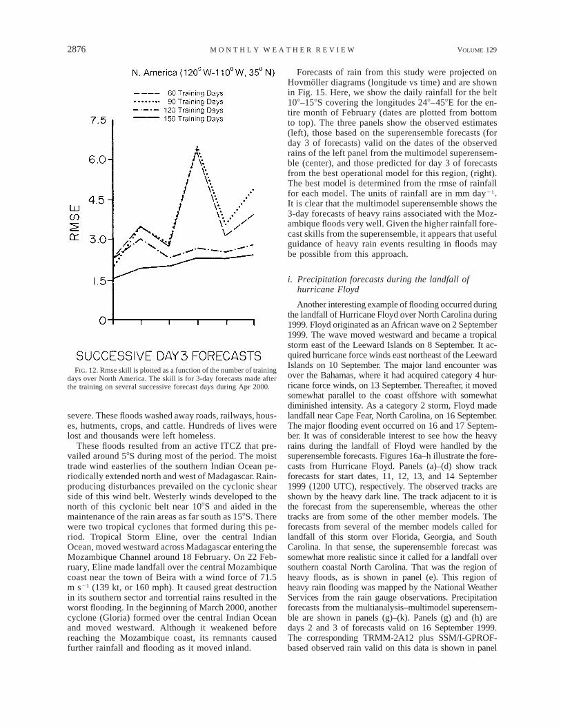
e. How many training days are needed for improvingprecipitation forecasts?

The results describing the number of training daysfor 3-day rainfall forecast skills over North America areshown in Fig. 12. We show the skills from 60 to 150days of training. It is apparent that there is a slow in-crease of skill as the number of days of training is in-creased. We believe that this is a function of the typeof rain-producing disturbances that prevail in a given


FIG. 9. Rmse of precipitation forecasts over different domains. The results for 6 member models, the ensemblemean, and the superensemble are displayed for 6 regions.

region. Over regions with a high degree of quasi-sta-tionary disturbances, such as the ITCZ, a lesser numberof training days (ø60 days) were sufficient to acquirea high skill for precipitation forecasts (Krishnamurti etal. 2000b). On the other hand, where there was an abun-dance of transient disturbances, such as over the mon-soon region, a large number of training days is needed.

f. Training with an arbitrary model’s GDAS rainfalldatasets

The improved results for the superensemble forecasts,shown earlier, came from using ‘‘best’’ rainfall estimates

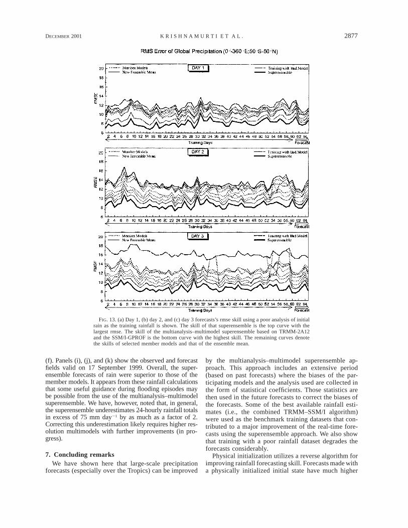
during the training phase. Best rainfall is here definedby the TRMM-and SSM/I-based estimates. One can askthe question, ‘‘What happens if the training were doneusing a lower quality rainfall estimate?’’ Forecast ver-ification must still be done with respect to the best rain-fall estimates, that is, the TRMM-2A12-and theSSM/I-GPROF-based estimates. Fig. 13a–c illustratesthe result of the rmse (based on 60 days of training and5 days of forecasts) starting January 2000. These areaveraged over the global belt from 508S to 508N. Thethick black lines show the results for the multimodel–multianalysis superensemble. Those errors are thesmallest compared to the bias-removed ensemble mean


FIG. 10. Percentage improvement (based on correlation) of the superensemble forecasts overthe ensemble mean, the best, and the poorest models.

(thin solid lines) and the selected member models (dot-ted lines). The long dashed lines with the largest errorsare the results of superensemble forecasts where thetraining was deliberately carried out using the initialrain (GDAS rain) of a poor model. That resulted in thelargest errors in the forecasts for days 1, 2, and 3. Itshould be noted that these skills depend strongly on thebenchmark rain rates that are used for training and fore-cast verification. We believe that TRMM-2A12-andSSM/I-GPROF-based rain rates are one of the betterproducts currently available for this purpose.

g. Relative performance among the rain-ratealgorithms

Ground validation experiments provide excellent da-tasets for the calibration of rain-rate algorithms. Thesedatasets are also most useful for testing the validity ofrain-rate algorithms. When one compares numericalweather prediction analyses with these algorithm prod-ucts, the model’s particular features also play an im-portant role in assessing how well such algorithm-basedrain rates fare with respect to the model’s results. Modelphysics, resolution, and dynamics always determine an


FIG. 11. Histograms showing percent improvement (based on correlation) of the superensemble forecast over the ensemble mean, the bestmodel, and the worst model for the global belt, 508S–508N.

equilibrium rainfall intensity state to which the forecastmodels spin up. Those rainfall intensities have more todo with the design of the numerical weather predictionmodels and less to do with the design of rainfall al-gorithms. Some of these individual model biases can bereduced by taking the multimodel superensemble ap-proach, which compensates for the growth or decay inthe spin up of rain rates from different models. Withinthe superensemble forecast strategy, we invoke a vasttraining period during which the model biases, with re-spect to a particular preassigned best rain-rate algorithm,are evaluated. That so-called best rain-rate descriptorwas selected as the TRMM-2A12 plus the SSM/I-GPROF algorithms following Kummerow et al. (1998).That choice was dictated by a consensus from theTRMM science team of NASA. Given that as a built-in feature for our training, the first-day forecasts (afterthe training) reflect the spun up values of the rain ratesfrom the superensemble (Fig. 14). These rain rates arecompared to the ‘‘observed’’ rain rate estimates fromsix different rain-rate algorithms. The six vertical barsshow, respectively, (a) the one-day forecast rain fromthe superensemble forecasts, (b) the observed rainfallestimate from the TMI-2A12 and SSM/I GPROF al-gorithm (TMI1SSM/I), (c) the observed rainfall esti-mate from the Ferraro et al. (1998) algorithms (Ferraro),(d) the observed rainfall estimate from Olson et al.(1990) algorithm (Olson), (e) the observed rainfall es-timates from the geostationary satellite-based algorithm

GEO of Turk et al. (2001), and (f) the observed rainfallestimates from the combined TRMM, SSM/I and thegeostationary satellite–based Turk algorithms (Turk etal. 2001).

The results shown in Fig. 14 are averages for theentire month of April 2000. These results are shown forrepresentative points over six selected domains: India,southeastern United States, Australia, China, westernPacific Ocean, and Africa. In all of these cases, we notethat the superensemble forecasts for day 1 closelymatches the observed rainfall estimates from TRMM–2A12 and the SSM/I-GPROF algorithms. The super-ensemble forecasts do not match the other algorithmsas closely. That has, of course, a lot to do with the choiceof the TRMM-2A12 plus SSM/I-GPROF for our train-ing. This is an important factor that determines the im-proved precipitation forecasts we report in this paper.

h. Mozambique floods

It is of considerable interest to ask whether the su-perensemble forecasts of rainfall can provide any usefulguidance for floods. Mostly the heavy rains that resultedin the recent Mozambique floods during February andMarch of the year 2000 resulted from heavy rains overMozambique and Zimbabwe. The headwaters of theLimpopo River over Zimbabwe experienced the heavi-est rainfall, which resulted in the cresting of the riverover southern Mozambique where the flooding was most


FIG. 12. Rmse skill is plotted as a function of the number of trainingdays over North America. The skill is for 3-day forecasts made afterthe training on several successive forecast days during Apr 2000.

severe. These floods washed away roads, railways, hous-es, hutments, crops, and cattle. Hundreds of lives werelost and thousands were left homeless.

These floods resulted from an active ITCZ that pre-vailed around 58S during most of the period. The moisttrade wind easterlies of the southern Indian Ocean pe-riodically extended north and west of Madagascar. Rain-producing disturbances prevailed on the cyclonic shearside of this wind belt. Westerly winds developed to thenorth of this cyclonic belt near 108S and aided in themaintenance of the rain areas as far south as 158S. Therewere two tropical cyclones that formed during this pe-riod. Tropical Storm Eline, over the central IndianOcean, moved westward across Madagascar entering theMozambique Channel around 18 February. On 22 Feb-ruary, Eline made landfall over the central Mozambiquecoast near the town of Beira with a wind force of 71.5m s21 (139 kt, or 160 mph). It caused great destructionin its southern sector and torrential rains resulted in theworst flooding. In the beginning of March 2000, anothercyclone (Gloria) formed over the central Indian Oceanand moved westward. Although it weakened beforereaching the Mozambique coast, its remnants causedfurther rainfall and flooding as it moved inland.

Forecasts of rain from this study were projected onHovmoller diagrams (longitude vs time) and are shownin Fig. 15. Here, we show the daily rainfall for the belt108–158S covering the longitudes 248–458E for the en-tire month of February (dates are plotted from bottomto top). The three panels show the observed estimates(left), those based on the superensemble forecasts (forday 3 of forecasts) valid on the dates of the observedrains of the left panel from the multimodel superensem-ble (center), and those predicted for day 3 of forecastsfrom the best operational model for this region, (right).The best model is determined from the rmse of rainfallfor each model. The units of rainfall are in mm day21.It is clear that the multimodel superensemble shows the3-day forecasts of heavy rains associated with the Moz-ambique floods very well. Given the higher rainfall fore-cast skills from the superensemble, it appears that usefulguidance of heavy rain events resulting in floods maybe possible from this approach.

i. Precipitation forecasts during the landfall ofhurricane Floyd

Another interesting example of flooding occurred duringthe landfall of Hurricane Floyd over North Carolina during1999. Floyd originated as an African wave on 2 September1999. The wave moved westward and became a tropicalstorm east of the Leeward Islands on 8 September. It ac-quired hurricane force winds east northeast of the LeewardIslands on 10 September. The major land encounter wasover the Bahamas, where it had acquired category 4 hur-ricane force winds, on 13 September. Thereafter, it movedsomewhat parallel to the coast offshore with somewhatdiminished intensity. As a category 2 storm, Floyd madelandfall near Cape Fear, North Carolina, on 16 September.The major flooding event occurred on 16 and 17 Septem-ber. It was of considerable interest to see how the heavyrains during the landfall of Floyd were handled by thesuperensemble forecasts. Figures 16a–h illustrate the fore-casts from Hurricane Floyd. Panels (a)–(d) show trackforecasts for start dates, 11, 12, 13, and 14 September1999 (1200 UTC), respectively. The observed tracks areshown by the heavy dark line. The track adjacent to it isthe forecast from the superensemble, whereas the othertracks are from some of the other member models. Theforecasts from several of the member models called forlandfall of this storm over Florida, Georgia, and SouthCarolina. In that sense, the superensemble forecast wassomewhat more realistic since it called for a landfall oversouthern coastal North Carolina. That was the region ofheavy floods, as is shown in panel (e). This region ofheavy rain flooding was mapped by the National WeatherServices from the rain gauge observations. Precipitationforecasts from the multianalysis–multimodel superensem-ble are shown in panels (g)–(k). Panels (g) and (h) aredays 2 and 3 of forecasts valid on 16 September 1999.The corresponding TRMM-2A12 plus SSM/I-GPROF-based observed rain valid on this data is shown in panel


FIG. 13. (a) Day 1, (b) day 2, and (c) day 3 forecasts’s rmse skill using a poor analysis of initialrain as the training rainfall is shown. The skill of that superensemble is the top curve with thelargest rmse. The skill of the multianalysis–multimodel superensemble based on TRMM-2A12and the SSM/I-GPROF is the bottom curve with the highest skill. The remaining curves denotethe skills of selected member models and that of the ensemble mean.

(f). Panels (i), (j), and (k) show the observed and forecastfields valid on 17 September 1999. Overall, the super-ensemble forecasts of rain were superior to those of themember models. It appears from these rainfall calculationsthat some useful guidance during flooding episodes maybe possible from the use of the multianalysis–multimodelsuperensemble. We have, however, noted that, in general,the superensemble underestimates 24-hourly rainfall totalsin excess of 75 mm day21 by as much as a factor of 2.Correcting this underestimation likely requires higher res-olution multimodels with further improvements (in pro-gress).

7. Concluding remarksWe have shown here that large-scale precipitation

forecasts (especially over the Tropics) can be improved

by the multianalysis–multimodel superensemble ap-proach. This approach includes an extensive period(based on past forecasts) where the biases of the par-ticipating models and the analysis used are collected inthe form of statistical coefficients. Those statistics arethen used in the future forecasts to correct the biases ofthe forecasts. Some of the best available rainfall esti-mates (i.e., the combined TRMM–SSM/I algorithm)were used as the benchmark training datasets that con-tributed to a major improvement of the real-time fore-casts using the superensemble approach. We also showthat training with a poor rainfall dataset degrades theforecasts considerably.

Physical initialization utilizes a reverse algorithm forimproving rainfall forecasting skill. Forecasts made witha physically initialized initial state have much higher


FIG. 14. Day 1 superensemble forecast of rain (mm day21) for representative points over 6 differentregions are compared to the observed estimates derived from different rain-rate algorithms fromTMI 1 SSM/I, Ferraro, Olson, GEO, and Turk forecasts. These are averaged for the entire monthof April 2000.

nowcasting skill for rainfall forecasts for day 1, andsomewhat higher skill for days 2 and 3, when comparedto operational model forecasts that do not deploy thisprocedure. This procedure requires observed rain-rateestimates according to which the physical initializationis addressed. The observed rain rates from the satellite-based microwave products (TMI, SSM/I) rely heavily

on the rain-rate algorithm that is used. The individualalgorithms appear to show differences in the 3-day fore-casts even though all other aspects of the model andinitial datasets were apparently kept the same. Thosedifferences arise largely from differences in heating,divergence, moisture, and pressure tendencies. Thus,differences in the initial rainfall provided a tag for the


FIG. 15. A Hovmoller diagram of daily precipitation (mm day21) on day 3 of forecasts during the Mozambique floods. Ordinate showsdays (bottom to top); abscissa denotes longitude. The three panels denote (left) observed rain (from TRMM-2A12 plus SSM/I GPROF);(middle) superensemble forecasts; (right) best operational model.


FIG. 16. (a)–(d) Track forecasts for Hurricane Floyd on different start dates. Heavy black line denotes official best track. The red lineadjacent to it is the superensemble forecast. The others are for some of the member multimodels. (e) Observed 5-day rainfall over NorthCarolina from Hurricane Floyd during 12–17 Sep 1999. (f)–(k) Observed, day 2, and day 3 superensemble-based precipitation forecastsduring the passage of Hurricane Floyd are shown. Two start dates of forecasts are illustrated here.


different versions of the multianalysis component of thesuperensemble. The multimodel components of the su-perensemble include the operational rainfall forecasts.In this paper, we have shown that the short range (1–3-day) precipitation forecast skills from the multiana-lysis–multimodel superensemble are higher than thoseof the (a) member models included in this exercise, (b)straightforward ensemble mean of the member models,and (c) bias-removed ensemble mean of the membermodels.

The multimodel forecasts are usually not bias-cor-rected when they are received. Given a model’s bias fordays 1, 2, and 3 of forecasts, we can correct the biasesof the individual models by simply adjusting the forecastmean values to corresponding observed mean values forthe past history of forecasts. Another approach to thebias correction of individual models is to perform aregression of past forecast variables of the single modelagainst observed models. That linear regression pro-vides a bias correction, which is somewhat differentfrom the adjustment of the mean. We have, in effect,examined the precipitation forecasts from (a) the mul-timodels, (b) ensemble mean of simple bias correctedindividual models, (c) ensemble mean of regression-based corrected individual models, and (d) superensem-ble proposed in this study.

We find that the precipitation forecast skill succes-sively improves as we move from (a) through (d). Wedo not present the results for the ensemble mean of bias-corrected individual models. Those were illustrated inKrishnamurti et al (2000a). Basically we noted that thesuperensemble performs better than the bias-correctedensemble mean of member models because assigning aweight of 1.0 to a poor model (after bias correction)does not make it comparable to the best model (afterbias correction). The superensemble assigns fractionalor even negative weights and is very selective. The re-moval of bias of poorer models does not appear to bringthem up to the levels of the best models, and assigningan equal weight to such models for the construction ofthe ensemble mean does not bring it to the level of theproposed superensemble. The latter benefits from thegeographically selective weights based on past perfor-mance. We have also addressed the issues of extremerain events (intensity greater than 75 mm day21), suchas those that occurred over the global Tropics in Apriland May 2000, during the landfall and flooding thatoccurred from Hurricane Floyd of 1999 and the Moz-ambique floods during February 2000. We show thatuseful forecast guidance may be available from the mul-tianalysis–multimodel superensemble for up to 3 days.The success of this study is attributed largely to therainfall estimates from TRMM, SSM/I products, and therain-rate algorithms that were developed in this context.

The global average improvement of the predictedrainfall by the superensemble of about 35% over thebias-removed ensemble mean (see Fig. 10a) came aboutfrom assigning a score of 0 for the ensemble mean and

a score of 100 for the best forecast. The ensemble meanis a product of the multimodel forecasts, whereas thesuperensemble includes past behavior of the model fore-casts as well. If the bias correction is made to each modeland a weight of 1.0 (uniformly over the globe) is as-signed to each model thereafter, then we find that thisensemble mean has a somewhat lower skill comparedto the proposed superensemble. That difference arisesfrom the fact that the latter assigns selective weights todifferent models (at any grid location). We found thatpoorer models, after a simple bias removal, do not per-form as well as the best model (after its bias removal).The selective weights [some 73 728 (384 3 192 lat/lon) times the number of member models for the pre-cipitation forecasts] appear to provide an edge for thesuperensemble over an ensemble mean (as is noted inFigs. 10 and 11).

The results shown in this paper demonstrate a modestimprovement over earlier work as is evident from Table2. Although the improvement in the equitable threatscores appear quite large, they should still be regardedas modest. Clearly further work is needed to improvethe mesoscale modeling of precipitation.

Further improvements in precipitation forecasts maybe possible from an extension of the proposed meth-odology:

1) Use of mesoscale multianalysis–multimodels for theconstruction of the superensemble, that is, use of ahigher-resolution family of models.

2) Further improvements in the remote sensing of rainrates from improved algorithms and ground valida-tion research. A follow-on mission (Global Precip-itation Mission) after TRMM is expected in the nextfive years. This mission will carry a constellation ofsatellites that would provide a much improved sam-pling of rainfall. This is expected to provide 3-hsampling of rainfall estimates. A considerable re-duction of errors is thus expected.

3) Further improvements in the cumulus parameteri-zation procedures among the member models. Useof explicit schemes and developing compatibility be-tween the model-based microphysical parameteri-zation and the satellite-based estimates of hydro-meteor components.

4) Further improvements in the data assimilation meth-odologies for the multimodels where the precipita-tion components are directly assimilated, for ex-ample, Treadon (1996), Hou et al. (2000), Tsuyuki(1996a,b; 1997). Most of these studies have reliedupon coarser resolution models. Further improve-ments should be possible with the use of variationaldata assimilation of rain rates using mesoscale mod-els.

It would be desirable to address the issue of ensemblespread, probabilistic forecast, and probability densityfunction (pdf ). The results of the superensemble fore-casts often reside well outside the results of the member


models and are quite different, by their nature, from anensemble mean. Thus, an ensemble spread of membermodels, although very useful for discussing the prop-erties of the ensemble mean, is not that simply relatedto the superensemble. The mathematical formulation ofthe pdf of the superensemble, for the precipitation fore-casts, will be addressed in a separate paper in the future.

The overall message of this study is that multiana-lysis–multimodel performs better than a single model.The percent improvement of the 3-day forecast rainfalldistributions over the current best model is quite large,between 40 and 120% over most areas. Thus, it wouldseem that this procedure could be useful for operationalweather prediction.

Acknowledgments. The research reported here wasfunded by NASA TRMM Grant NAG5-4729 andNAG5-9662, NSF Grant ATM-9710336 and ATM-9910526, and NOAA Grant NA86GP0031 andNA77WA0571.

We wish to also acknowledge the modeling groupsfrom ECMWF, NCEP, BMRC, JMA, NRL (NOGAPS),and RPN for providing the global datasets. This workcould not have been completed without the assistanceof the TRMM/TSDIS data centers, especially the sup-port from Erich Stocker and Tony Stocker. We also wishto thank the U.S. Air Force Global Weather Center atOmaha, Nebraska, and the Naval Laboratory in Mon-terey, California, for the SSM/I datasets.

APPENDIX A

Outline of the FSU Global Spectral Model

The global model used in this study is identical tothat used in Krishnamurti et al. (1991). The followingis an outline of the global model:

(a) Independent variables: (x, y, s, t).(b) Dependent variables: vorticity, divergence, sur-

face pressure, vertical velocity, temperature,and humidity.

(c) Horizontal resolution: Triangular 126 waves.(d) Vertical resolution: 14 layers between roughly

10 and 1000 mb.(e) Semi-implicit time differencing scheme.(f ) Envelope orography (Wallace et al. 1983).(g) Centered differences in the vertical for all var-

iables except humidity, which is handled by anupstream differencing scheme.

(h) Fourth-order horizontal diffusion (Kanamitsuet al. 1983).

(i) Kuo-type cumulus parameterization (Krishna-murti et al. 1983a).

(j) Shallow convection (Tiedke 1984).(k) Dry convective adjustment.(l) Large-scale condensation (Kanamitsu 1975).(m) Surface fluxes via similarity theory (Businger

et al. 1971).

(n) Vertical distribution of fluxes utilizing diffu-sive formulation where the exchange coeffi-cients are functions of the Richardson number(Louis 1979).

(o) Longwave and shortwave radiative fluxesbased on a band model (Harshvardan and Cor-setti 1984; Lacis and Hansen 1974).

(p) Diurnal cycle.(q) Parameterization of low, middle, and high

clouds based on threshold-relative humidity forradiative transfer calculations.

(r) Surface energy balance coupled to the similar-ity theory (Krishnamurti et al. 1991).

(s) Nonlinear normal mode initialization—5 ver-tical modes (Kitade 1983).

(t) Physical initialization (Krishnamurti et al.1991).

APPENDIX B

Creation of a Superensemble Prediction at a GivenGrid Point

N

S 5 O 1 a (F 2 F ),O i i ii51

where S 5 superensemble prediction, 5 time meanOof observed state, ai 5 weight for model i, i 5 modelindex, N 5 number of models, i 5 time mean of pre-Fdiction by model i, and Fi 5 prediction by model i. Theweights ai are computed at each grid point by mini-mizing the following function:

t2train

2G 5 (S 2 O ) ,O t tt50

where O 5 observed state, t 5 time, and t2train 5length of training period.

REFERENCES

Adler, R. F., and A. J. Negri, 1988: A satellite infrared technique toestimate convective and stratiform precipitation. J. Appl. Me-teor., 27, 30–51.

——, A. J. Negri, P. R. Keehn, and I. A. Hakkarinen, 1993: Estimationof monthly rainfall over Japan and surrounding waters from acombination of low-orbit microwave and geosynchronous IRdata. J. Appl. Meteor., 32, 335–356.

——, G. J. Huffman, and P. R. Keehn, 1994: Global tropical rainestimates from microwave-adjusted geosynchronous infrareddata. Remote Sens. Rev., 11, 125–152.

Berg, W., W. Olson, R. Ferraro, S. J. Goodman, and F. J. LaFontaine,1998: An assessment of the first and second generation navyoperational precipitation retrieval algorithms. J. Atmos. Sci., 55,1558–1575.

Businger, J. A., J. C. Wyngard, Y. Izumi, and E. F. Bradley, 1971:Flux profile relationship in the atmospheric surface layer. J. At-mos. Sci., 28, 181–189.

Ferraro, R. R., 1997: Special sensor microwave imager derived globalrainfall estimates for climatological applications. J. Geophys.Res., 102 (D14), 16 715–16 735.


——, and G. F. Marks, 1995: The development of SSM/I rain-rateretrieval algorithms using ground-based radar measurements. J.Atmos. Oceanic Technol., 12, 755–770.

——, E. A. Smith, W. Berg, and G. J. Huffman, 1998: A screeningmethodology for passive microwave precipitation retrieval al-gorithms. J. Atmos. Sci., 55, 1583–1600.

Hakkarinen, I. M., and R. F. Adler, 1988: Observations of precipi-tating convective systems at 92 and 183 GHz: Aircraft results.Meteor. Atmos. Phys., 38, 164–182.

Harshvardan, and T. G. Corsetti, 1984: Longwave parameterizationfor the UCLA/GLAS GCM. NASA Tech. Memo. 86072, God-dard Space Flight Center, Greenbelt, MD, 52 pp.

Hou, A. Y., D. V. Ledvina, A. M. da Silva, S. Q. Zhang, J. Joiner,R. M. Atlas, G. J. Huffman, and C. D. Kummerow, 2000: As-similation of SSM/I-derived surface rainfall and total precipi-table water for improving the GEOS analysis for climate studies.Mon. Wea. Rev., 128, 509–537.

Kanamitsu, M., 1975: On numerical prediction over a global tropicalbelt. Dept. of Meteorology Rep. 75-1, The Florida State Uni-versity, Tallahassee, FL, 282 pp.

——, K. Tada, K. Kudo, N. Sato, and S. Ita, 1983: Description ofthe JMA operational spectral model. J. Meteor. Soc. Japan, 61,812–828.

Kasahara, A., A. P. Mizzi, and L. J. Donner, 1994: Diabatic initial-ization for improvement in the tropical analysis of divergenceand moisture using satellite radiometric imagery data. Tellus,46A, 242–264.

Kitade, T., 1983: Nonlinear normal mode initialization with physics.Mon. Wea. Rev., 111, 2194–2213.

Krishnamurti, T. N., Y. Ramanathan, H. L. Pan, R. J. Pasch, and J.Molinari, 1980: Cumulus parameterization and rainfall rates I.Mon. Wea. Rev., 108, 465–472.

——, S. Low-Nam, and R. Pasch, 1983a: Cumulus parameterizationand rainfall rates II. Mon. Wea. Rev., 111, 816–828.

——, S. Cocke, R. Pasch, and S. Low-Nam, 1983b: Precipitationestimates from raingauge and satellite observations summer MO-NEX. Rep. 83-7, Department of Meteorology, The Florida StateUniversity, Tallahassee, FL, 373 pp.

——, J. Xue, H. S. Bedi, K. Ingles, and D. Oosterhof, 1991: Physicalinitialization for numerical weather prediction over the tropics.Tellus, 43AB, 53–81.

——, G. Rohaly, and H. S. Bedi, 1994: On the improvement ofprecipitation forecast skill from physical initialization. Tellus,46A, 598–614.

——, C. M. Kishtawal, T. LaRow, D. Bachiochi, Z. Zhang, C. E.Williford, S. Gadgil, and S. Surendran, 1999: Improved weatherand seasonal climate forecasts from multimodel superensemble.Science, 285, 1548–1550.

——, ——, D. W. Shin, and C. E. Williford, 2000a: Improving trop-ical precipitation forecasts from a multianalysis superensemble.J. Climate, 13, 4217–4227.

——, and Coauthors, 2000b: Multimodel ensemble forecasts forweather and seasonal climate. J. Climate, 13, 4196–4216.

Kummerow, C., W. S. Olson, and L. Giglio. 1996: A simplifiedscheme for obtaining precipitation and vertical hydrometeor pro-files from passive microwave sensors. IEEE Trans. Geosci. Re-mote Sens., 34, 1213–1232.

——, W. Barnes, T. Kozu, J. Shiue, and J. Simpson, 1998: The Trop-ical Rainfall Measuring Mission (TRMM) sensor package. J.Atmos. Oceanic Technol., 15, 809–817.

——, and Coauthors, 2000: The status of the Tropical Rainfall Mea-

suring Mission (TRMM) after two years in orbit. J. Appl. Me-teor., 39, 1965–1982.

Lacis, A. A., and J. E. Hansen, 1974: A parameterization for theabsorption of solar radiation in the Earth’s atmosphere. J. Atmos.Sci., 31, 118–133.

Louis, J. F., 1979: A parametric model of vertical eddy fluxes in theatmosphere. Bound.-Layer Meteor., 17, 187–202.

Marecal, V., and J. F. Mahfouf, 2000: Variational retrieval of tem-perature and humidity profiles from TRMM precipitation data.Mon. Wea. Rev., 128, 3853–3866.

Olson, W. S., F. J. LaFontaine, W. L. Smith, and T. H. Achtor, 1990:Recommended algorithms for the retrieval of rainfall rates in thetropics using the SSM/I (DMSP-8). Manuscript, University ofWisconsin, Madison, WI, 10 pp.

——, C. Kummerow, G. M. Heymsfield, and L. Giglio, 1996: Amethod for combined passive-active microwave retrievals ofcloud and precipitation profiles. J. Appl. Meteor., 35, 1763–1789.

Puri, K., and M. J. Miller, 1990: The use of satellite data in thespecification of convective heating for diabatic initialization andmoisture adjustment in numerical weather prediction models.Mon. Wea. Rev., 118, 67–93.

Shin, D. W., and T. N. Krishnamurti, 1999: Improving precipitationforecasts over the global tropical belt. Meteor. Atmos. Phys., 70(1–2), 1–14.

Tao, W. K., and J. Simpson, 1993: Goddard cumulus ensemble model.Part I: Model description. TAO: Terr. Atmos. Oceanic, 4, 35–72.

Tiedtke, M., 1984: The sensitivity of the time-mean large-scale flowto cumulus convection in the ECMWF model. Proc., Workshopon Convection in Large-Scale Numerical Models. Reading, Unit-ed Kingdom, ECMWF, 297–316.

Treadon, R. E., 1996: Physical initialization in the NMC global dataassimilation system. Meteor. Atmos. Phys., 60, 57–86.

——, 1997: Assimilation of satellite derived precipitation estimateswithin the NCEP. Ph.D. dissertation, The Florida State Univer-sity, Tallahassee, FL, 348 pp.

Tripoli, G. J., 1992: A nonhydrostatic model designed to simulatescale interaction. Mon. Wea. Rev., 120, 1342–1359.

Tsuyuki, T., 1996a: Variational data assimilation in the Tropics usingprecipitation data. Part I: Column model. Meteor. Atmos. Phys.,60, 87–104.

——, 1996b: Variational data assimilation in the Tropics using pre-cipitation data. Part II: 3D model. Mon. Wea. Rev., 124, 2545–2561.

——, 1997: Variational data assimilation in the Tropics using pre-cipitation data. Part III: Assimilation of SSM/I precipitationrates. Mon. Wea. Rev., 125, 1447–1464.

Turk, J., C.-S. Liou, S. Qiu, R. Scofield, M. Ba, and A. Gruber, 2001:Capabilities and characteristics of rainfall estimates from geo-stationary-and geostationary1microwave-based satellite tech-niques. Preprints, Symp. or Precipitation Extremes: Prediction,Impacts, and Responses, Albuquerque, NM, Amer. Meteor. Soc.,191–194.

Wallace, J. M., S. Tibaldi, and A. J. Simmons, 1983: Reduction ofsystematic forecast errors in the ECMWF model through theintroduction of envelope orography. Quart. J. Roy. Meteor. Soc.,109, 683–718.

Xie, P., and P. A. Arkin, 1998: Global monthly precipitation estimatesfrom satellite-observed outgoing longwave radiation. J. Climate,11, 137–164.

Yanai, M., S. Esbensen, and J. H. Chu, 1973: Determination of bulkproperties of tropical cloud clusters from large-scale heat andmoisture budgets. J. Atmos. Sci., 30, 611–627.

Real-Time Multianalysis–Multimodel Superensemble Forecasts...

Documents

Transcript of Real-Time Multianalysis–Multimodel Superensemble Forecasts...