Real Exchange Rates, International Trade and Macroeconomic

Real Exchange Rates, International Trade and

Macroeconomic Fundamentals

Winnie Wing-Yin Choi

Department of Economics

Stanford University ∗

January 2005

Job Market Paper

Abstract

Many studies on real exchange rates have found little relationship between macroeconomicfundamentals and real exchange rates in the short- to medium-run. This is widely-known as the‘exchange rate disconnect puzzle’. This paper derives a new equilibrium condition between realexchange rates, international trade and macroeconomic fundamentals for a wide class of gen-eral equilibrium models, allowing for goods market frictions with proportional transport costsand non-traded goods, and a wide variety of asset market structures. The key is to link theprice indices through prices of traded goods. If consumption bundle is a constant-elasticity-of-substitution bundle between the home traded good, foreign imports and the non-traded good,then there is an equilibrium relationship between real exchange rates and relative composite-good consumptions plus two other factors: the ratio of bilateral trade flows and the ratio ofdomestic traded good consumptions. These additional trade factors arise from bilateral in-tratemporal allocations. The intratemporal elasticity of substitution between goods plays a keyrole in real exchange rate determination.

I present empirical evidence that this trade-based representation of real exchange rates sig-nificantly improves on the standard consumption-ratio formula in understanding actual realexchange rates movements. In particular, it identifies preference shocks or incomplete marketsas possible explanations for the Backus-Smith (1993) puzzle by breaking the tight relationshipbetween real exchange rates and relative consumptions.

∗Corresponding e-mail: [email protected]. I am grateful to my dissertation advisor Narayana Kocherlakota forhis guidance and support. I also thank David Backus, Timothy Cogley, Raquel Fernandez, Doireann Fitzgerald, GitaGopinath, Robert Hall, Peter Hansen, Timothy Kehoe, Pete Klenow, Hanno Lustig, Ellen McGrattan, Ronald McK-innon, Maurice Obstfeld, Fabrizio Perri, Esteban Rossi-Hansberg, Thomas Sargent, Michele Tertilt, Mark Wright,Anthony Chung, Benjamin Malin and participants of the Stanford Macroeconomics Lunch and Stanford InternationalEconomics Seminar for their helpful comments and suggestions.

1 Introduction

A large number of studies over the past twenty years have discovered virtually no relationship be-tween real exchange rates and macroeconomic fundamentals, such as relative consumptions, moneysupplies, GDPs, etc. This is widely known as the ‘exchange rate disconnect puzzle’. Obstfeld andRogoff (2000) describe the situation as, ‘Exchange rates are remarkably volatile relative to any

models we have of underlying fundamentals, such as interest rates, outputs, money supplies and no

model seems to be very good at explaining exchange rates even ex post’. Frankel and Rose (1995)also state, “We, like much of the profession, are doubtful of the value of further time series modeling

of exchange rates at high or medium frequencies using macroeconomic models”. In addition, manyempirical studies have documented the purchasing power parity puzzles. Real exchange rates areextremely volatile compared with macroeconomic variables. Real exchange rates are also highlypersistent. Consensus half-lives of real exchange rates are between three and five years, implying along time for innovations to be arbitraged away.

This paper studies real exchange rate determination for a wide class of general equilibriummodels. I show that real exchange rate can be expressed as a function of international trade flows,relative domestic traded goods consumptions, and relative composite goods consumptions. I callthis equilibrium condition the trade-based representation of real exchange rates. I demonstrateempirically that for a wide variety of cross-country pairs, actual real exchange rates are highlycorrelated with the trade-based representation. In particular, for the major trading partners withthe U.S, the correlations between actual real exchange rates and their trade-based representationsare over 0.8. Thus, I find that in the data, real exchange rates are in fact closely connected tointernational trade flows and macroeconomic fundamentals, as predicted by economic theory.

I derive the trade-based representation of real exchange rates as follows. The real exchangerate is an intra-temporal relationship between national price levels. The price indices across twocountries can be quite different, due to non-traded goods or different compositions of goods withinthe consumption bundle. I relate these two price indices through the prices of traded goods acrosscountries. I set up a class of general equilibrium models of international trade with three basicassumptions. (i) There are multiple goods. Each country is only endowed with one of the tradedgoods. (ii) Utility is strictly increasing and strictly concave in consumption. The consumptionaggregator is homogeneous of degree 1 with respect to the goods within the consumption bundle,strictly concave, time-separable and satisfies Inada conditions. (iii) Prices are perfectly flexible. Allcountries take prices as given in competitive markets.

A key result for any general equilibrium models satisfying the above assumptions is a no-arbitrage pricing condition for each traded good. Each country i is indifferent between selling itsown traded good i at home at the domestic price pii, or selling the same good i at another country

1

j at a price pji that takes into account the proportional transport costs. Assuming only η fractionper unit of goods shipped is delivered at the foreign border, the no-arbitrage condition is pii = pjiη.Without any transport costs, this no-arbitrage condition is the ‘Law of One Price’.

From the no-arbitrage pricing condition, the real exchange rate can then be expressed as a ratioof two relative prices: the price of a traded good to price index in country i versus the price of thesame traded good to price index in country j. These relative prices are related to the marginalutilities of that traded good to the relative marginal utilities of the consumption bundles. I thenderive the theoretical equilibrium condition between real exchange rates, international trade andmacroeconomic variables. If the country i’s composite consumption ci is a constant-elasticity-of-substitution aggregator with respect to consumptions of the home traded good di, imports fromcountry j mij and non-traded good ni with 1

ρ as the intratemporal elasticity of substitution betweenall goods, then the real exchange rate is

ln e = ρ

(12

lndj

di+

12

lnmji

mij+ ln

ci

cj

)(1)

Equation (1) is an equilibrium condition between real exchange rates and relative compositegood consumptions ci

cjplus two other factors: the ratio of bilateral trade flows mji

mijand the ratio

of domestic good consumptions across country pairs dj

di. The additional trade factors enter from

bilateral intratemporal allocations of traded goods to their respective consumption bundles. Therelative compositions of the consumption bundles and the intra-temporal elasticity of substitutionbetween goods 1

ρ are crucial for real exchange rate determination. I call the right-hand-side ofEquation (1) the trade-based representation of real exchange rate.

The trade-based representation in Equation (1) is valid for any economy that satisfies the threekey assumptions. Hence it is valid for any specification of intertemporal preferences, intertempo-ral trade and asset markets, goods market frictions of proportional transport costs or non-tradedgoods. It is also robust for any specification of production possibilities and the sources of shocks.These other features of the economy determine how real exchange rates and real quantities moveover time. My theoretical analysis is that no matter what are the sources of the fluctuations, realexchange rates and real quantities should co-move together according to the equilibrium conditionin Equation (1).

I evaluate the fit of equilibrium condition (1) using data from 1980 to 1998 for 13 major indus-trialized economies. I find that the trade-based representation fit the data well. For close tradingpartners with the U.S, such as Canada, Japan, U.K, France and Germany, the raw data correlationsfor the trade-based representation with the actual real exchange rates in log levels are over 0.8. Forall 78 bilateral pairs in the sample, over 50% of them have over 0.7 raw data correlations for actualreal exchange rates and the trade-based representation. These correlations remain high even when

2

I filter out the long-run components in the data using HP-filter or band-pass-filter.

It is useful to contrast my trade-based representation with the consumption-based representationderived by Backus and Smith (1993). They show that if asset markets are complete and if thereare no preference shocks, then real exchange rates and relative consumptions must satisfy theequilibrium condition:

ln e = γ lnci

cj+ constant (2)

where γ is the coefficient of risk aversion in the utility function, and the constant term representsthe ratio of initial Pareto-Negishi weights of the social planner across countries i and j. I call theright-hand-side of Equation (2) the consumption-based representation of real exchange rates.

I show that the consumption-based representation have a low, often negative correlation withactual real exchange rates for most bilateral country pairs in the OECD1, while the trade-basedrepresentation have positive correlations with actual real exchange rates for most bilateral pairs inthe sample. I also show that the consumption-based representation is not as volatile as actual realexchange rates unless γ is above 2.5, whereas the trade-based representation matches the volatil-ity of actual real exchange rates if the elasticity of substitution between goods ρ equals 1. Thisis because additional trade factors add to the volatility of the trade-based representation of realexchange rates. Finally, I show that the consumption-based representation is not cointegrated withreal exchange rates, while the trade-based representation is cointegrated with real exchange rateswith a long-run relationship.

Why are the empirical results for the trade-based representation a significant improve comparedto the consumption-based representation in Backus and Smith (1993)? I demonstrate that undercomplete markets and no preference shocks, the trade-based representation of real exchange rate isthe same as the consumption-based representation. It is because Pareto optimality requires eachtraded good to be allocated such that the ratio of marginal utilities of each traded good to allcountries equals to a constant that corresponds to the initial social planner’s weights. Therefore,the empirical failure of the consumption-based representation (i.e. the Backus-Smith (1993) puz-zle) relative to the trade-based representation indicates that either asset markets are incompleteor there are different preference shocks across countries. With incomplete markets or preferenceshocks, the trade-based representation can help explain the low correlation between real exchangerates and relative consumptions as the additional trade factors are negatively-covaried with relativeconsumptions.

1Backus and Smith (1993) provide empirical evidence that the correlations between real exchange rates and relativeconsumptions are close to zero on average and even quite negative for certain countries. This empirical evidence oflow correlations between relative consumptions and real exchange rates is also documented in other studies such asChari, Kehoe and McGrattan (2002), Ravn (2001), etc. This is known as the Backus-Smith puzzle.

3

These results indicate that theoretically and empirically, real exchange rates are closely con-nected to international trade flows and macroeconomic fundamentals. However, while the analysisshows that intra-temporal trade in goods market is related to real exchange rate determination,there are still open questions about the true source of real exchange rate fluctuations and theinter-temporal properties of real exchange rates. In particular, we need better understanding ofthe asset markets and the dynamics of international trade to enhance our understanding for theinter-temporal properties of real exchange rates.

Most studies of real exchange rate determination in general equilibrium models have found aclose theoretical link between real exchange rates and relative consumptions. This arises from thefirst order conditions for agents choosing between domestic and foreign goods, or choosing betweendomestic and foreign assets (e.g. Backus and Smith 1993, Chari, Kehoe and McGrattan (2002),Atkeson Alvarez and Kehoe (2002), Sercu and Uppal (2003), etc). Other research papers thatstudy deviations from purchasing power parity usually assume some type of goods market frictionsor asset market frictions. For example, Dumas (1992) and Obstfeld and Rogoff (2000) suggest thattransport costs in international trade plays a key role for volatile and persistent deviations fromparity. Betts and Devereux (2000) and Chari, Kehoe and McGrattan (2002) suggest that mone-tary shocks interacting with sticky goods prices can generate volatile and persistent real exchangerate fluctuations. Alvarez, Atkeson and Kehoe (2002) suggest that endogenously segmented assetmarkets leads to volatile and persistent exchange rates. There are fewer studies that have offeredtheoretical explanations to the Backus-Smith puzzle. Chari, Kehoe and McGrattan (2002) suggestthat some forms of asset market frictions are required to break the link between real exchange ratesand relative consumptions.

Section 2 presents a class of general equilibrium models of international trade. The naturalimplication from the model is a no-arbitrage pricing condition for each traded good. I derive thetrade-based representation for real exchange rate from this no-arbitrage pricing condition. Section3 empirically evaluates how this trade-based representation performs in understanding actual realexchange rate movements, especially the PPP volatility and persistence puzzles and the Backus-Smith puzzle. Section 4 concludes.

2 General Equilibrium Model of International Trade and Real Ex-

change Rates

This section sets up a class of general equilibrium models of international trade. With three basicassumptions of (i) complete specialization of traded goods endowments, (ii) standard assumptionon preferences and (iii) flexible prices, a natural implication is a no-arbitrage pricing condition for

4

each traded good. The individual goods prices can aggregate up to form the price index for eachcountry. I derive the real exchange rates as the ratio of national price indices of composite goodconsumptions.

2.1 The Model: Key Assumptions

Time is discrete t = 1, ..., T .2 At time t, the state st is realized and it can take on any elementfrom the finite set S. Let st = (s1, ..., st) denote the history for state st in time t. There are I

countries, i = 1...I, located in I different geographical locations. There is a representative agent ineach country.

Multiple Goods. Complete Specialization of Traded Good Endowment. There are I

perishable traded consumption goods. Country i is only endowed with one traded good yi(st) > 0.The traded good endowment process yi(st) is drawn on a positive finite set Yi.

There can also be a non-traded good yiN (st) ≥ 0 endowed in each country i. The non-tradedgood endowment process is drawn on a non-negative finite set YiN . Each country consumes acomposite good which is a consumption bundle of the I traded goods and the non-traded good(the composite good comprises of I + 1 goods). To consume the other non-endowed traded goods,country i would need to purchase the other traded goods from abroad.

Preferences The utility function Ui(ci(st)) : <+ → < of the representative agent in countryi at date t state st can be country-specific and can take on the most general form given com-posite good consumption ci ≥ 0. Assume Ui is strictly increasing and strictly concave in ci (i.e.U ′

i(ci) > 0, U ′′i (ci) < 0). This general form of utility can include the standard time-separable CRRA

utility functions, non-time separable utilities such as habit persistence, non-state separable utilitiessuch as Kreps-Porteus of Epstein-Zin preferences, etc3.

The consumption aggregator ci(st) = ci(di(st), mij(st)j 6=i,j∈1,...,I, ni(st)) : <+×<I−1+ ×<+ →

<+ consists of date t state st consumption of the traded good endowed in their own country(di(st) ≥ 0), consumption of the foreign traded good endowed by country j (mij(st) ≥ 0), con-sumption of the non-traded good endowed in country i (ni(st) ≥ 0). Assume the consumption

2It can be a static economy with T = 1 or dynamic economy with T > 1 with asset market trading. I focus theanalysis of dynamic economies in this paper. If asset markets are complete or exogenously incomplete, T can be finiteor infinite. If asset markets are endogenously incomplete subject to solvency constraints similar to Alvarez-Jermann(2000), I require T to be infinite for reputation to play a role in determining allocations.

3This general form of preference also includes utility functions with more arguments such as utility with leisureor money-in-the-utility functions.

5

bundle is homogeneous of degree 14. Assume ci(st) is strictly concave with respect to each of itscomponents5, twice differentiable and satisfies Inada conditions with respect to the imported good(i.e. limmij→0

∂ci(st)

∂mij(st) = ∞ ,limmij→∞∂ci(s

t)∂mij(st) = 0). Assume the consumption bundle ci(st) is

time-separable with respect to di(st), mij(st)j 6=i, ni(st) and does not depend on past consump-tions of each of the components di(st−τ ), mij(st−τ )j 6=i, ni(st−τ ) for τ > 0.

Flexible Prices. Goods prices are perfectly flexible. All countries take prices as given in com-petitive markets.

2.2 Goods Market and Asset Market

In each country, there are I + 1 goods market open for each I traded goods and the non-tradedgoods6. Goods market shipping can be subject to a proportional (iceberg) transport costs. Foreach unit of good shipped, only η(st) ∈ (0, 1] fraction of the good is delivered at the foreign border.Country i can buy a certain traded good j either in the country i (home) market after the good isshipped to home country, or country i can buy it directly in country j’s (foreign) market and shipthe good back home itself.7

Let xij(st) ≥ 0 be the export of traded good i from country i to country j. The consumptionsof each good within the consumption bundle of country i is as follows

di(st) = yi(st)−∑

j 6=i

xij(st), i 6= j (3)

mij(st) = η(st)xji(st), i 6= j (4)

ni(st) = yiN (st) (5)

where (3) is the market clearing condition of traded good i, (4) is import-export relationship fortraded good j with transport costs and (5) is the market clearing condition for non-traded good i.

4For scalar value ξ,

ci(ξdi(st), ξmij(s

t)j 6=i, ξni(st)) = ξci(di(s

t), mij(st)j 6=i, ni(s

t))

This assumption is required so that the expenditure on the consumption bundle is the same as the sum of expenditureon the individual goods pi(s

t)ci(st) = pii(s

t)di(st) +

Pj 6=i pij(s

t)mij(st) + piN (st)ni(s

t). Differentiate with respectto ξ and evaluate the derivative at ξ = 1:

ci(st) =

∂ci(st)

∂di(st)di(s

t) +Xj 6=i

∂ci(st)

∂mij(st)mij(s

t) +∂ci(s

t)

∂ni(st)ni(s

t)

5The strict concavity for ci(st) with respect to di(s

t), mij(st), ni(s

t) is to guarantee that there is always a positiveamounts of exports and imports. If ci(s

t) is linear (e.g. ci(st) = di(s

t) +P

j 6=i mij(st) + ni(s

t)), there exists a cone

of no shipping similar to Dumas (1992) and the real exchange rates would fluctuate between η(st) and 1η(st)

.6There are a total of I(I + 1) markets in the world.7Apart from the iceberg transport costs, there are no further limitations to arbitrage for traded goods.

6

The notations for goods prices are as follows. Let pij(st) be the price of traded good j in thecountry i market. Let piN (st) be the price of non-traded good i in country i.

There can be a wide variety of asset market structures. I assume the net asset holdings in statest are summarized by the wealth accumulated Wi(st).8 This can encompass complete markets,endogenously incomplete markets or exogenously incomplete markets9.

Each country i solves the following maximization problem in time t state st

maxdi,mij ,nii6=j

Ui(ci(st)) (6)

where

ci(st) = ci(di(st), mij(st)j 6=i, ni(st))

mij(st) ≥ 0

subject to the sequential budget constraints for country i

pii(st)di(st) +∑

j 6=i

pij(st)mij(st) + piN (st)ni(st) = pii(st)yi(st) + piN (st)yiN (st) + Wi(st) (7)

Assume existence of equilibrium. The definition of competitive equilibrium is as follows.

Definition of Equilibrium: An equilibrium is a sequence of allocations ci(st), di(st), mij(st),ni(st)i6=j,i,j=1....I , a sequence of goods prices pij(st), piN (st)i,j=1....I such that

(i) Each country i solves the maximization problem (6).(ii) Goods market clearing is satisfied for each traded good and non-traded good (i.e. Equations(3) to (5)).

8The details of the asset markets are as follows. Assume there are H securities available. There is no cost intrading securities in the asset markets. Let qh(st) be the price of the security h in terms of consumption bundle ci.at time t state st with a payoff of ah(st+1) in terms of consumption bundle ci at time t + 1 state st+1. Let bih(st)be country i’s holding of security h at time t state st. The net asset holdings or wealth accumulated Wi(s

t) equalsPHh=1[bih(st−1)ah(st)− bih(st)qh(st)]. The assets can also be in terms of other bundles (e.g. composite good j: cj)

or in terms of specific goods within the consumption bundle. In a static economy, there are no asset market tradesand Wi = 0.

9Asset holdings are subject to a general form for K ≤ H borrowing limits φik(bi1(st), ..., biH(st)) ≥ 0 for k = 1...K

depending on the asset market structures, where φik : <H → R+ is a linear function. If asset markets are complete,there is a full set of state-contingent securities H = S. Asset holdings are subject to natural borrowing limits thatnever bind in equilibrium. If asset markets are endogenously incomplete similar to Alvarez and Jermann (2000),there are still H = S securities available for trading, but asset holdings are subject to state-contingent endogenousborrowing constraints Bi(s

t): φik(bi1(st), ..., biH(st)) =

PHh=1 bih(st) − Bi(s

t) ≥ 010 and K = 1. If asset marketsare exogenously incomplete, H < S. If there are K ≤ H additional borrowing or short-sale constraints of Bk assetholdings are restricted by the K constraints of φik(bi1(s

t), ..., biH(st)) = bik(st)−Bk ≥ 0 for k = 1...K.

7

2.3 No-arbitrage Pricing Condition and Trade-based Representation of Real

Exchange Rates

In this section, I focus on the subset of equilibrium conditions from goods market optimization.

Proposition 1: In an equilibrium with strictly positive trade flows at all states (i.e. mij(st) > 0),the no-arbitrage condition pii(st) = pji(st)η(st) holds.

Proposition 1 is a no-arbitrage pricing condition for any traded good i. This no-arbitrage con-dition implies all countries face common prices for the same good adjusted for transport costs; andcountry i is indifferent between selling traded good i at home or selling traded good i in country j

at a price that takes into account the transport costs.

The intuition for Proposition 1 is as follows. Suppose pii(st) < pji(st)η(st), then country i orcountry j would have an incentive to buy the traded good i in country i and sell traded good i inthe country j market and make a profit. In this case, demand for traded good i increases and theprice of good traded i in country i increases until it equilibrates to pji(st)η(st). A similar argumentholds for the opposite case pii(st) > pji(st)η(st). If there is no transport cost (η(st) = 1), thisno-arbitrage goods market pricing condition is the ‘Law of One Price’.

Since our goal is to understand real exchange rate movements as the ratio of price indicesof the composite goods of two countries, I shall construct below the price index pi(st) for eachcountry i from individual goods prices. The consumption-based price index for country i pi(st) isdefined as the minimum expenditure for the unit consumption bundle ci, given individual goodsprices pii(st), pij(st), piN (st).11 Since the consumption bundle ci(st) is CES with respect todi(st), mij(st)j 6=i, ni(st), I can express the price index for country i as follows.

pi(st) ≡ pii(st)di(st) +∑

j 6=i pij(st)mij(st) + piN (st)ni(st)ci(st)

From this definition of the price index, the sequential budget constraint (7) can be rewritten as

pi(st)ci(st) = pii(st)yi(st) + piN (st)yiN (st) + Wi(st) (8)

The price of a consumption bundle can be found from the first order condition with respect toci(st) in the new budget constraint (8).

pi(st)σi(st) = U ′i(ci(st)) (9)

The real exchange rate between countries i and j is defined as the ratio of price indices across

11Definition from Obstfeld and Rogoff (1996).

8

countries12

eij(st) ≡ pj(st)pi(st)

=U ′

j(cj(st))U ′

i(ci(st))σi(st)σj(st)

(10)

To derive our equilibrium relationship between real exchange rates and allocations, our goal isto express the ratio of the Lagrange Multipliers of country i and country j’s budget constraintsσi(s

t)σj(st) in terms of allocations. The two national price indices can be very different due to non-tradedgoods or different preferences within the consumption bundle. However, it is possible to link thetwo national price indices through prices of traded goods. The prices of traded good i sold incountry i and country j can be found from the first order conditions of country i’s problem withrespect to di in budget constraint (7) and country j’s problem with respect to mji

pii(st) =U ′

i(ci(st))σi(st)

∂ci(st)∂di(st)

,pii(st)pi(st)

=∂ci(st)∂di(st)

(11)

pji(st) =U ′

j(cj(st))σj(st)

∂cj(st)∂mji(st)

,pji(st)pj(st)

=∂cj(st)

∂mji(st)(12)

Equation (11) shows that if more traded good i is allocated to country i’s bundle, then therelative price of traded good i to country i’s price level decreases. Similarly, Equation (12) showsthat if more traded good i is allocated to country j’s bundle, then the relative price of traded goodi to country j’s price level decreases. I can then calculate the real exchange rate by applying theno-arbitrage pricing condition in Proposition 1 to (11) and (12). I arrive at the main propositionof this paper.

Proposition 2: The equilibrium condition between real exchange rates and allocations is

eij(st) =(

∂ci(st)/∂di(st)∂cj(st)/∂mji(st)

) 12(

∂ci(st)/∂mij(st)∂cj(st)/∂dj(st)

) 12

(13)

=(

pii(st)/pi(st)η(st)pji(st)/pj(st)

) 12(

η(st)pij(st)/pi(st)pjj(st)/pj(st)

) 12

(14)

I denote the right hand side of Proposition 2 as the trade-based representation of real exchangerates ln eT . It can be decomposed into two parts.

eTij(s

t) = (∂ci(st)/∂di(st)

∂cj(st)/∂mji(st))

12

︸︷︷︸alloc. of good i

(∂ci(st)/∂mij(st)∂cj(st)/∂dj(st)

)12

︸︷︷︸alloc. of good j

The first part indicates how country i allocates traded good i intra-temporally between di(st) and

12Suppose we have a model with nominal exchange rates εij (price of currency i in terms of currency j), the realexchange rate between countries i and j is defined as eij = εij

pj

pi. In this model, I assume there is no money for any

countries or they use the same cash for transactions.

9

mji(st). The second part in Proposition 2 indicates how country j allocates traded good j intra-temporally between mij(st) and dj(st). The ‘1/2’ power is due to our assumption that the transportcost from country i to country j is the same as the transport cost from country j to country i (i.e.ηij(st) = ηji(st) = η(st)).

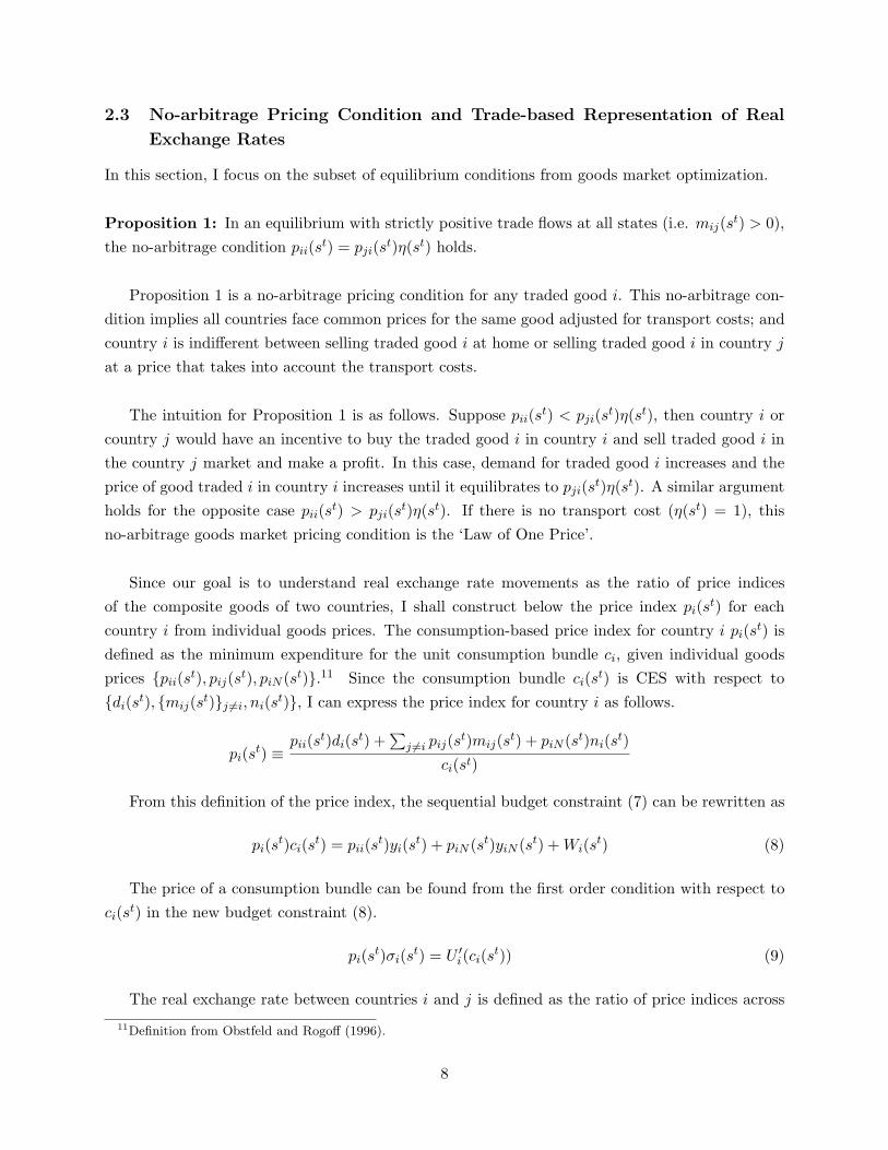
The key insight for Proposition 2 is to relate price indices across countries by price of tradedgoods.

eij(st) ≡ pj(st)pi(st)

=pii(st)/pi(st)

η(st)pji(st)/pj(st)=


The second equality is the ratio of the price of traded good i relative to price index in country i

versus the price of the same traded good i relative to the price index in country j, adjusted fortransport cost. Similarly, the third equality is the ratio of the price of traded good j relative toprice index in country i adjusted for transport cost, versus the price of the same traded good i

relative to the price index in country j. Equation (14) in Proposition 2 links the prices of bothtraded goods to the price indices by substituting out the transport cost.

Existing studies on real exchange rates focus mostly on the relative price indices of consumptionbundles pj(s

t)pi(st) and ignore the effects from price components for the specific goods (i.e. pii(s

t)η(st)pji(st)

and η(st)pij(st)

pjj(st) ). While these price components for specific goods are equal to 1 in equilibrium fromProposition 1, they have implications in relating real exchange rates and the allocations of specificgoods within the bundle.

The trade-based representation of real exchange rate in Proposition 2 is valid for any econ-omy that satisfies the three key assumptions in Section 2.1. The composition of specific goodsdi,mij , ni within the consumption bundle ci is crucial in the determination of real exchangerates. While real exchange rate is still defined as the ratio of marginal utilities of consumptionbundles, the form of utility function Ui does not enter directly in Proposition 2. It affects realexchange rates only indirectly through the allocations. Hence the trade-based representation isrobust to a wide class of time-consistent preferences, such as the HARA class of utility functions,non-time separable utilities (e.g. external or internal habit persistence), recursive utilities or non-state separable utilities. It is also robust to utility functions with non-separability with leisure ormoney-in-the-utility functions. Both countries can indeed have very different utility functions andthe trade-based representation in Proposition 2 still holds.

This trade-based representation is robust to more general frictions of goods market of country-specific, time-varying proportional transport costs. It is also robust to different asset market struc-tures such as complete markets, endogenously incomplete or exogenously incomplete markets. Ishall explore in the next section how asset market structures relate to real exchange rates determi-

10

nation.

The trade-based representation also holds in a production economy with capital and laborbecause it is mainly a spot relationship from the intra-temporal optimal allocations in state st. Italso holds in an economy with money and flexible prices. The no-arbitrage pricing condition wouldbe pii = εijpjiη and εijpjj = pijη where εij is the nominal exchange rate of currency i in termsof currency j. The real exchange rate eij is eij = εij

pj

pi. It is easy to verify the same equilibrium

condition for real exchange rates in (13) from this no-arbitrage pricing condition. These otherfeatures of the economy determine how real exchange rates and real quantities move over time.My theoretical analysis is that no matter what are the sources of the fluctuations, real exchangerates and real quantities should co-move together according to the trade-based representation inProposition 2.

2.4 Real Exchange Rates, Asset Market Structures and Preference Shocks

The derivation for the trade-based representation of real exchange rate in Proposition 2 does notrely on the first order conditions on asset holdings. This explains its robustness across a widevariety of asset market structures. Asset markets, however, affect real exchange rates indirectlythrough the allocations.

Complete Markets, No Preference Shocks. If markets are complete, there exists a socialplanner for optimal allocations. Let αi be the social planner’s initial weight on country i. Theconsumption-based representation of real exchange rate is

eC =αj

αi

U ′j(cj)

U ′i(ci)

By the first and second welfare theorems, the allocations in the planner’s problem are the same asthe decentralized market problem if the planner’s weight is the inverse of the Lagrange Multiplier ofthe sequential budget constraint αi = 1

σi(st) . In complete markets, the ratio σi(st)

σj(st) would correspondto the initial ratios of social planner’s weights αj

αi. Pareto optimality requires each traded good to

be allocated such that the marginal utilities of each traded good to countries i and j equal to aconstant that corresponds to the initial ratio of planner’s weights.

U ′i(ci(st))

U ′j(cj(st))

∂ci(st)/∂di(st)η(st)∂cj(st)/∂mji(st)

=U ′

i(ci(st))U ′

j(cj(st))η(st)∂ci(st)/∂mij(st)

∂cj(st)/∂dj(st)=

σi(st)σj(st)

=αj

αi= constant

Therefore if markets are complete and if there are no preference shocks, the trade-based repre-sentation eT has the same value as the consumption-based representation of real exchange rate eC

11

in Backus and Smith (1993).

eC =αj

αi

U ′j(cj(st))

U ′i(ci(st))

=∂ci(st)/∂di(st)

η(st)∂cj(st)/∂mji(st)=

η(st)∂ci(st)/∂mij(st)∂cj(st)/∂dj(st)

= eT

Under complete markets, there is complete consumption smoothing across traded goods and realexchange rate fluctuations should be due to non-traded goods. This confirms Balassa and Samuel-son’s (1964) proposition that if country i has a higher shock to traded good relative to non-tradedgoods and the prices of traded goods equalize across countries, the relative price of non-tradedgoods is higher and country i’s real exchange rate appreciates.

Incomplete Markets, Preference Shocks. I shall demonstrate that preference shocks or incom-plete markets can be possible explanations for the Backus-Smith’s puzzle. Suppose the utility forcountry i in state st is δi(st) ci(s

t)1−γ

1−γ where δi(st) is the preference shock to country i’s consumptionbundle, then the real exchange rate is

eij(st) =δj(st)δi(st)

σi(st)σj(st)

(ci(st)cj(st)

)γ

(15)

Empirically, the correlations between real exchange rates and relative consumptions are verylow, even negative for many country-pairs. Equation (15) shows that the low correlation can bedue to either different preference shocks across countries δj(s

t)δi(st) or incomplete asset markets for

time-varying ratio of Lagrange Multipliers of the budget constraints σi(st)

σj(st) .13 Combining (15) and

Proposition 2 imply the following equilibrium condition

δj(st)δi(st)

σi(st)σj(st)

=(


) 12(

∂ci(st)/∂mij(st)∂cj(st)/∂dj(st)

) 12(

cj(st)ci(st)

)γ

(16)

The higher the relative preference shocks δj(st)

δi(st) for country j versus country i, the more countryj desires to consume compared to country i and the higher the allocations for the traded goods i

and j to country j’s bundle versus to country i’s bundle. This would be reflected in a increase inthe relative ratios of ∂ci(s

t)/∂di(st)

∂cj(st)/∂mji(st) and ∂ci(st)/∂mij(s

t)∂cj(st)/∂dj(st) .

If markets are endogenously incomplete, there also exists a social planner and the welfaretheorems still hold (Alvarez and Jermann (2000)). However, the social planner’s weights can betime-varying according to changes in promised utilities. Applying the no-arbitrage pricing condition

13Kehoe and Perri (2002) suggest that endogenously incomplete markets help to explain international businesscycles in a single-good model with production. Corsetti, Dedola and Leduc (2002) demonstrate numerically thatincomplete market with goods market frictions may explain the low correlation of real exchange rates and relativeconsumptions. Kollman (1995) shows that the fluctuations of consumption and real exchange rates are consistentwith incomplete asset markets.

12

to (11) and (12),

σi(st)σj(st)

=U ′

i(ci(st))U ′

j(cj(st))

(∂ci(st)/∂di(st)

η(st)∂cj(st)/∂mji(st)

)

If country i has a good shock such that its enforcement constraint binds, its promised utilityincreases accordingly. Country i enjoys more consumption (i.e. di(st),mij(st), ni(st) increases)which lowers the marginal utility of consumption with respect to domestic traded goods (i.e.U ′

i(ci(st)) ∂ci(st)

∂di(st) decreases). σi(st)

σj(st) decreases. Therefore when country i has a good shock in yi

and yiN , (1) country i increases its composite good consumption relative to country j, the marginalutility of composite good consumption decreases relative to that of country j (i.e. U ′i(ci(s

t))U ′j(cj(st))

de-

creases) and price index for country i pi(st) decreases; (2) the price level pi(st) in country i canincrease relative to country j because of a higher promised utility (i.e. σi(s

t)σj(st) decreases). Since

real exchange rates relate to both components of U ′i(ci(st))

U ′j(cj(st))and σi(s

t)σj(st) and these two forces work

in opposite directions, real exchange rate for country i can either appreciate or depreciate. Theoptimal allocations would be such that that the ratio of marginal utilities of traded good i andtraded good j for country i and country j reflect the changes of promised utilities for the countries.

If markets are exogenously incomplete, the optimal allocations would be such that the marginalutilities for traded good i and traded good j for country i and country j changes according tothe wealth accumulated for each country. The higher the wealth accumulated for country i, thelower the ratio of both U ′i(ci(s

t))U ′j(cj(st))

and σi(st)

σj(st) . There can be either real exchange rates appreciation

or depreciation. Under exogenously incomplete markets, σi(st)

σj(st) would also be time-varying andthe trade-based representation would differ in value from the consumption-based representation ofreal exchange rate (i.e. ln eT 6= ln eC). Time-varying ratio of Lagrange Multipliers of the budgetconstraint σi(s

t)σj(st) due to incomplete markets can be a possible explanation for the low correlation

between real exchange rates and relative consumptions across countries

2.5 Examples: Preliminaries for Empirical Analysis

We consider a special case of the consumption aggregator for our empirical analysis in the nextsection. Given a consumption bundle ci(st), we allow for arbitrary strictly increasing and strictlyconcave utility function Ui(ci). Suppose the composite consumption good is constant elasticity ofsubstitution with the same elasticity of substitution between goods 1

ρ for both countries, i.e.

ci(st) = [ω1di(st)1−ρ +∑

j 6=i,j∈1..Iω2mij(st)1−ρ + ω3ni(st)1−ρ]

11−ρ (17)

where ω1, ω2, ω3 > 0 indicate the bias in the preference in consuming the domestically endowedtraded good di(st), versus the imported foreign good mij(st) versus the non-traded good ni(st).

13

The trade-based representation of real exchange rate from (13) is

eT (st) =(ω1ci(st)/di(st))

ρ2

(ω2cj(st)/mji(st))ρ2︸︷︷︸

good i

(ω2ci(st)/mij(st))ρ2

(ω1cj(st)/dj(st))ρ2︸︷︷︸

good j

(18)

eT (st) =(

dj(st)di(st)

) ρ2(

mji(st)mij(st)

) ρ2(

ci(st)cj(st)

)ρ

(19)

There is an equilibrium condition between real exchange rates and relative composite goodconsumptions plus two other factors: the ratio of bilateral trade flows mji(s

t)mij(st) and the ratio of

consumptions of domestically-endowed traded goods dj(st)

di(st) . The elasticity of substitution betweengoods 1

ρ within the bundle plays a key role in real exchange rates determination.

Since the additional trade factors are negatively correlated with relative consumptions, thetrade-based representation of real exchange rate has the potential to explain the Backus-Smithpuzzle that real exchange rates and relative consumptions have low or even negative correlation inthe data.

cov(ln eT (st), lnci(st)cj(st)

) =ρ

2Cov(ln

dj(st)di(st)

, lnci(st)cj(st)

)︸︷︷︸

<0

+ρ

2Cov(ln

mji(st)mij(st)

, lnci(st)cj(st)

)︸︷︷︸

<0

+ρV ar(lnci(st)cj(st)

)

3 Empirical Analysis

3.1 Data

This section performs empirical analysis for understanding actual real exchange rate movements.I obtain quarterly data from 13 major industrialized countries between 1980 to 1998: Australia,Canada, Japan, Switzerland, United Kingdom, Austria, Finland, France, Germany, Italy, Portugal,Spain and the U.S. There are a total of 78 bilateral country-pairs. The data sources are from In-ternational Financial Statistics, OECD Quarterly National Accounts, Direction of Trade Statisticsand Datastream. A detailed description of the data sources and construction of variables are in theData Appendix.

3.2 Actual Real Exchange Rates, Consumption-based and Trade-based Repre-

sentations of Exchange Rates

Let ln eAijt be the log of actual real exchange rate from the data. Let ln eC

ijt be the log consumption-based representation of real exchange rates. If the utility function is CRRA with γ as the coefficientof relative risk aversion, the consumption-based representation is the ratio of relative real consump-

14

Table 1: Raw Data: Corr(ln eA; ln eC) and Corr(ln eA; ln eT )Raw Data Canada Japan U.K. France Germany

U.S. Corr(ln eA; ln eC) -0.367 -0.651 -0.431 -0.073 -0.526Corr(ln eA; ln eT ) 0.887 0.874 0.801 0.864 0.907

tions,

ln eCijt = γ ln

cit

cjt+ constant

Let ln eTijt be the trade-based representation of real exchange rates derived in Proposition 2. If the

elasticity of substitution between all goods in the consumption bundle is 1ρ

ln eTijt = ρ

(12

lndjt

dit+

12

lnmjit

mijt+ ln

cit

cjt

)

To highlight the results of this paper, I focus on five major trading partner countries againstthe U.S.: Canada, U.K., Japan, France and Germany. Table 1 shows these correlations in the rawdata14. Most of the correlations for ln eA and ln eC are very low and negative in many countrypairs. This confirms the ‘Backus-Smith’ puzzle that the correlations of real exchange rates andrelative consumptions are very low. On the contrary, the correlations for ln eA and ln eT are muchhigher. For the major trading partners against the U.S, the raw data Corr(ln eA, ln eT ) are over0.8 . This higher correlation is because of the higher correlation of actual real exchange rate andthe two other trade factors: the ratio of consumption in domestically-endowed good (ln dj

di) and the

ratio of bilateral trade flows (ln mji

mij).

The details for the correlations for all bilateral pairs are in the Appendix. For 50% of all 78bilateral pairs, the raw data Corr(ln eA, ln eT ) are over 0.7. This is a significant improvement overCorr(ln eA, ln eC) in which only 1% have correlations over 0.7.

I also show the correlations with filters of different frequencies. I select the first-difference filterto focus on the short-term correlations, the band-pass filter for the medium-term correlations andthe HP-filter for the long-term correlations. For the HP-filter, the smoothing parameter is 1600for quarterly data. I focus on the cyclical component correlations after detrending. The band passfilter admits frequencies between 6 and 32 quarters. The moving average parameter for the bandpass filter has 12 leads/lags.

Table 2 shows the correlations of Corr(ln eA, ln eC) and Corr(ln eA, ln eT ) with different filters for

14Notice that these correlations do not depend on the parameter values of γ for ln eC and ρ for ln eT .

15

Table 2: First-difference filtered data, Band-pass filtered data, HP-filtered data: Corr(ln eA; ln eC)and Corr(ln eA; ln eT )

Base Country: U.S. Canada Japan U.K. France GermanyFirst Differences Corr(∆ ln eA;∆ ln eC) 0.021 0.056 0.008 -0.190 0.019

Corr(∆ ln eA; ∆ ln eT ) 0.495 0.618 0.250 0.496 0.596Band-pass Filtered Corr(ln eA; ln eC) 0.008 0.196 -0.150 -0.425 -0.105

Corr(ln eA; ln eT ) 0.908 0.755 0.681 0.883 0.802HP-Filtered Data Corr(ln eA; ln eC) -0.056 0.340 -0.109 -0.122 0.060

Corr(ln eA; ln eT ) 0.756 0.733 0.475 0.721 0.767

major trading partners against the U.S. The correlation in first differences for Corr(∆ ln eA;∆ ln eC)is almost zero for most trading partners of U.S. In general, Corr(∆ ln eA, ∆ln eT ) are lower thanin log levels, but they are positive and higher than Corr(∆ ln eA,∆ ln eC).

The correlations with the band-pass filter and the HP-filter are similar to Table 1. The cor-relations between the band-passed-filtered actual real exchange rates and the band-passed-filteredtrade-based representation are over 0.68 for these countries. The correlations between the HP-filtered actual real exchange rates and HP-filtered trade-based representation are over 0.47 forthese countries.

Figure 1 shows the histograms for the densities of Corr(ln eA, ln eC) (left figures) and Corr(ln eA,ln eT ) (right figures) for the raw data, first-differenced data, HP-filtered and band-pass-filtered datafor all 78 bilateral pairs in the sample. The figures show that Corr(ln eA, ln eT ) has much highercorrelations in general than Corr(ln eA, ln eC).

3.3 Real Exchange Rate Puzzles

3.3.1 The Volatility Puzzle

Empirically real exchange rates are much more volatile than relative consumptions. The volatilityof the standard consumption-based log real exchange rates is the volatility of relative consumptionsadjusted for the coefficient of relative risk aversion.

V ar(ln eCijt) = γ2V ar(ln

cit

cjt)

The variance of the trade-based log real exchange rate is

V ar(ln eTijt) = ρ2[

14V ar(ln

djt

dit) +

14V ar(ln

mjit

mijt) + V ar(ln

cit

cjt) +

12Cov(ln

djt

dit, ln

mjit

mijt)

+ Cov(lndj

di, ln

cit

cjt) + Cov(ln

mjit

mijt, ln

cit

cjt)]

16

−1 −0.5 0 0.5 10

20

40Histogram: Corr(ln eA, ln eC)

−1 −0.5 0 0.5 10

20

40Histogram: Corr(ln eA, ln eT)

−1 −0.5 0 0.5 10

20

40Histogram: Corr(ln deA, ln deC)

−1 −0.5 0 0.5 10

20

40Histogram: Corr(ln deA, ln deT)

−1 −0.5 0 0.5 10

20

40

Histogram: Corr(ln eABP

, ln eCBP

)

−1 −0.5 0 0.5 10

20

40

Histogram: Corr(ln eABP

, ln eTBP

)

−1 −0.5 0 0.5 10

20

40

Histogram: Corr(ln eAHP

, ln eCHP

)

−1 −0.5 0 0.5 10

20

40

Histogram: Corr(ln eAHP

, ln eTHP

)

CorrelationsCorrelations

Figure 1: Histogram for the Corr(ln eA, ln eC) (left figures) and Corr(ln eA, ln eT ) (right figures). First rowof figures: raw data. Second row of figures: First-differenced data. Third row of figures: Band-pass filtereddata. Fourth row of figures: HP-filtered data.

17

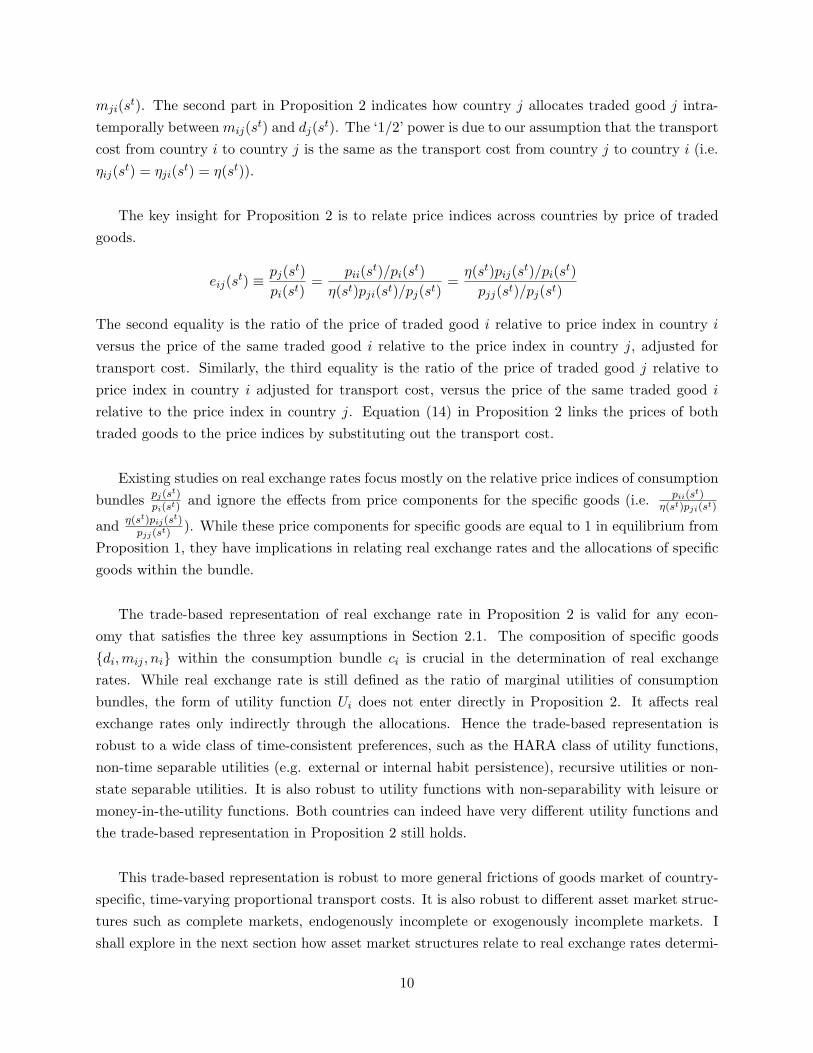
γ = 2, ρ = 1 Canada Japan U.K. France GermanyU.S. var(ln eA) 0.008 0.052 0.020 0.026 0.028

var(ln eC) 0.010 0.011 0.014 0.005 0.042var(ln eT ) 0.033 0.032 0.031 0.027 0.018

Table 3: Volatility of real exchange rates: var(ln eA), var(ln eC) and var(ln eT ).

γ = 2, ρ = 1 Var(ln(dj

di)) Var(ln(mji

mij)) Var(ln( ci

cj))

Canada 0.118 0.017 0.002Japan 0.009 0.153 0.001U.K. 0.047 0.073 0.001

France 0.006 0.125 0.003Germany 0.020 0.082 0.007

Table 4: Breakdown of volatility of real exchange rates.

Table 3 compares var(ln eA), var(ln eC) and var(ln eT ). Assume that the coefficient of risk aver-sion is the same for all countries and γ = 2. Assume the inverse of the elasticity of substitutionis the same for all countries and ρ = 1. Although the value of ρ is below γ, the volatility of thetrade-based representation matches the high volatility of actual real exchange rates quite well15.The breakdown of the variance of the trade-based representation is shown in Table 4. The varianceof the components var(ln dUS

di) and var(ln mUS,i

mi,US) are much higher than var(ln ci

cUS).

3.3.2 The Persistence Puzzle

Real exchange rates are highly persistent. Consensus half-lives of real exchange rates are aboutthree to five years16. For the consumption-based representation, the correlation of real exchangerates today and tomorrow is equal to the correlation of relative consumptions between today andtomorrow: Corr(ln eC

ijt, ln eCijt+1) = Corr(ln cijt

cjt, ln cit+1

cjt+1) . There are nine covariance components

15The details for var(ln eA), var(ln eC) and var(ln eT ) for all bilateral pairs are listed in Table 14 in the Appendix.16Taylor (2001) points out that many PPP tests in the literature may be subject to temporal aggregation and

non-linearity biases. The half-life estimates would tend to bias upwards.

18

Canada Japan U.K. France GermanyU.S. corr(ln eA

t ; ln eAt+1) 0.968 0.955 0.913 0.930 0.927

corr(ln eCt ; ln eC

t+1) 0.978 0.961 0.985 0.959 0.989corr(ln eT

t ; ln eTt+1) 0.983 0.930 0.900 0.908 0.949

Table 5: Persistence of real exchange rates: corr(ln eAt ; ln eA

t+1), corr(ln eCt ; ln eC

t+1)andcorr(ln eT

t ; ln eTt+1).

for the persistence of the trade-based representation of real exchange rates Corr(ln eTijt, ln eT

ijt+1).17

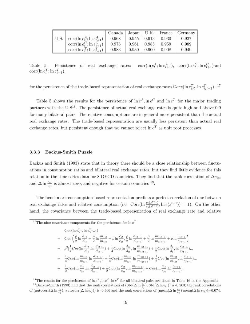
Table 5 shows the results for the persistence of ln eA, ln eC and ln eT for the major tradingpartners with the U.S18. The persistence of actual real exchange rates is quite high and above 0.9for many bilateral pairs. The relative consumptions are in general more persistent than the actualreal exchange rates. The trade-based representation are usually less persistent than actual realexchange rates, but persistent enough that we cannot reject ln eT as unit root processes.

3.3.3 Backus-Smith Puzzle

Backus and Smith (1993) state that in theory there should be a close relationship between fluctu-ations in consumption ratios and bilateral real exchange rates, but they find little evidence for thisrelation in the time-series data for 8 OECD countries. They find that the rank correlation of ∆eijt

and ∆ ln citcjt

is almost zero, and negative for certain countries 19.

The benchmark consumption-based representation predicts a perfect correlation of one betweenreal exchange rates and relative consumption (i.e. Corr(ln ci(s

t+1)cj(st+1)

, ln e(st+1)) = 1). On the otherhand, the covariance between the trade-based representation of real exchange rate and relative

17The nine covariance components for the persistence for ln eT

Cov(ln eTijt, ln eT

ijt+1)

= Cov

ρ

2ln

djt

dit+

ρ

2ln

mjit

mijt+ ρ ln

cit

cjt,ρ

2ln

djt+1

dit+1+

ρ

2ln

mjit+1

mijt+1+ ρ ln

cit+1

cjt+1

= ρ2[

1

4Cov(ln

djt

dit, ln

djt+1

dit+1) +

1

4Cov(ln

djt

dit, ln

mjit+1

mijt+1) +

1

2Cov(ln

dj

di, ln

cit+1

cjt+1)...

+1

4Cov(ln

mjit

mijt, ln

djt+1

dit+1) +

1

4Cov(ln

mjit

mijt, ln

mjit+1

mijt+1) +

1

2Cov(ln

mjit

mijt, ln

cit+1

cjt+1)...

+1

2Cov(ln

cit

cjt, ln

djt+1

dit+1) +

1

2Cov(ln

cit

cjt, ln

mjit+1

mijt+1) + Cov(ln

cit

cjt, ln

cit+1

cjt+1)]

18The results for the persistence of ln eA, ln eC , ln eT for all bilateral pairs are listed in Table 16 in the Appendix.19Backus-Smith (1993) find that the rank correlations of (Std(∆ ln ci

cj), Std(∆ ln eij)) is -0.263; the rank correlations

of (autocorr(∆ ln cicj

), autocorr(∆ ln eij)) is -0.466 and the rank correlations of (mean(∆ ln cicj

) mean(∆ ln eij))=0.074.

19

Canada Japan U.K. France GermanyU.S. corr(ln eA; ln ci/cj) -0.367 -0.651 -0.431 -0.073 -0.526

corr(ln eC ; ln ci/cj) 1 1 1 1 1corr(ln eT ; ln ci/cj) -0.645 -0.772 -0.765 -0.186 -0.617

Table 6: Correlation between ln eA, ln eC , ln eT and relative consumptions.

consumptions is

Cov(ln eTit, ln

cit

cjt) = Cov(

ρ

2ln

djt

dit+

ρ

2ln

mjit

mijt+ ρ ln

cit

cjt, ln

cit

cjt)

=ρ

2Cov(ln

djt

dit, ln

cit

cjt)

︸︷︷︸<0

+ρ

2Cov(ln

mjit

mijt, ln

cit

cjt)

︸︷︷︸<0

+ρV ar(lncit

cjt)

Since cit includes dit,mijt as components in the bundle, the two covariance terms Cov(ln djt

dit, ln cit

cjt)

and Cov(ln mjit

mijt, ln cit

cjt) are negative in theory and also negative in the data. The intuition for the

negative covariance is due to the fact that both countries allocate their traded goods intratempo-rally relative to country i and country j’s bundles. This relative allocations of specific goods toconsumption bundles lead to the negative covariances for Cov(ln djt

dit, ln cit

cjt) and Cov(ln mjit

mijt, ln cit

cjt).

The comparison for corr(ln eA, ln citcjt

), corr(ln eC , ln citcjt

) and corr(ln eT , ln citcjt

) for major tradingpartners against the U.S. is reported in Table 6.20 It is clear from the table that the trade-basedrepresentation is much better in matching the low correlation between actual real exchange ratesand relative consumptions.

3.4 Panel Estimation

This section estimates the coefficient of relative risk aversion γ from the consumption-based rep-resentation of real exchange rates ln eC and inverse of elasticity of substitution between goods ρ

from the trade-based representation ln eT . Most international business cycle models parametrize γ

to be between 2 and 521. For the studies estimating the elasticity of substitution between goods,the general conclusion is that the elasticity of substitution between traded goods is higher than 1(ρ < 1)22, but the elasticity of substitution between traded and non-traded goods is lower than 1

20The details for the correlations between ln eA, ln eC , ln eT and relative consumptions for all bilateral pairs arelisted in the Appendix (Table 17).

21Backus, Kehoe and Kydland (1992) use a value of 2 for γ for their international real business cycle model. AlvarezAtkeson and Kehoe (2002) parametrize γ to be 2 to illustrate the interest rate and exchange rate dynamics. Chari,Kehoe and McGrattan (2002) use a value of 5 to match up the volatility of real exchange rates and volatility ofrelative consumptions.

22Obstfeld and Rogoff (2000) summarize from recent trade studies that elasticity of import demand with respectto price (relative to the overall domestic consumption basket) is around 5 to 6. Chari, Kehoe and McGrattan (2002)state the most reliable studies in the literature for the elasticity of substitution between home and foreign good is

20

(ρ > 1)23. As the consumption bundle ci in our model include both traded goods and non-tradedgoods, I expect that the estimated inverse of elasticity of substitution ρ between 0.15 to 2.3 to beconsistent with other studies in the literature.

Since our model requires that the elasticity of substitution 1ρ be a constant such that the con-

sumption aggregator ci is CES with respect to di, mijj 6=i, ni, using U.S. as the base country, Iestimate the inverse of the elasticity of substitution ρ to be equal for all the countries in our sample.I perform the estimation under a balanced panel for the five major trading partners against theU.S. (N = 5) with T=76 observations for each country-pair between 1980:1-1998:4.The panel regressions on the consumption-based and the trade-based representations of real ex-change rates are

ln eAiUSt = γ

(ln

cit

cUSt

)+ δCDi + εCit, E(εCitε

′Cit) = ΩεC (20)

ln eAiUSt = ρ

([12

lndUSt

dit+

12

lnmUSit

miUSt+ ln

cit

cUSt

])+ δT Di + εTit, E(εTitε

′T it) = ΩεT (21)

The dependent variable is the actual real exchange rate ln eAiUSt of country i at time t where

i = 1..N , t = 1...T . The explanatory variable is ln cicUS

for the consumption-based representationof real exchange rates, and 1

2 ln dUSdi

+ 12 ln mUSi

miUS+ ln ci

cUSfor the trade-based representation of real

exchange rates. Di represents a matrix of variables that vary across countries but for each countryare constant across periods. This represents the time-invariant country-specific (fixed) effect24.δC , δT represents the vector of coefficients for the dummy variables Di. ρ and γ are our coefficientsof interest. εCit, εTit are the error structures of the disturbance terms. The standard errors areNewey-West (1987) heteroscedasticity and autocorrelation consistent with four lags using quarterlydata.

The results of the panel regressions for log levels with country dummies for quarterly raw dataare reported in Table 7. The estimate γ estimated from relative consumptions is negatively sig-nificant at -1.09. This is again inconsistent with the basic assumption of a positive coefficient ofrelative risk aversion. The estimate ρ from the trade-based representation is 0.97. It is quite closeto the Cobb-Douglas case for the unit elasticity of substitution between all goods. The R2 is higherfor the trade-based representation of real exchange rate at 0.697.

Figure 2 shows the comparison for ln eA, ln eC (left graphs) and ln eA, ln eT (right graphs)for two major trading partners against the U.S.: Canada and Japan. The upper graphs is for

between 1 to 2.23Tesar (1993) and Stockman and Tesar (1995) estimate that the elasticity of substitution between traded and

non-traded goods is 0.44.24I need to control for the fixed effects because the numeraires for the country bundle versus the U.S. bundle are

different.

21

Quarterly Data γ R2

Consumption-based Representation -1.085 0.183(0.152)

ρ R2

Trade-based Representation 0.970 0.697(0.044)

Table 7: Panel regressions for log levels with country dummies using quarterly raw data as-suming all countries have the same γ and the same ρ. Top panel: Explanatory variable is theconsumption-based representation of real exchange rates ln eA

iUSt = γ(ln citcUSt

)+δCDi+εCit. Bottompanel: Explanatory variable is the the trade-based representation of real exchange rate: ln eA

iUSt =ρ([12 ln dUSt

dit+ 1

2 ln mUSitmiUSt

+ ln citcUSt

]) + δT Di + εit. Let Xit be the explanatory variables on the right-hand-side. Total number of observations: 380, where N = 5 and T = 76. The coefficient estimatefor (γ, ρ) is

PNi=1

PTt=1(Xit−Xi)(Yit−Yi)PN

i=1

PTt=1(Xit−Xi)2

where Yi = 1T

∑Tt=1 Yit, Xi = 1

T

∑Tt=1 Xit. The variance for

(γ, ρ) is (∑N

i=1

∑Tt=1(Xit− Xi)2)−1Ω(

∑Ni=1

∑Tt=1(Xit− Xi)2)−1 where Ω is Newey-West (1987) het-

eroscedasticity and autocorrelation consistent matrix with 4 lags. Ω = Ω0+∑p

j=1(1− jp+1)(Ωj+Ω′j) ,

Ω0 = 1NT

∑Ni=1

∑Tt=1(εit⊗(Xit−Xi))2 and Ωj = 1

N

∑Ni=1

1T

∑Tt=j+1(εit⊗(Xit−Xi))(εi,t−j⊗(Xi,t−j−

Xi))′. R2 is calculated as 1−PN

i=1

PTt=1 u2

itPNi=1

PTt=1(yit−yi)2

Canada/U.S. and the lower graphs are for Japan/U.S. It can be seen that there is a much morepositive correlation between ln eA, ln eT than ln eA, ln eC. This result generalizes to many othercountries. Figure 3 illustrates graphically the actual real exchange rates against the consumption-based representation of real exchange rates for all countries in our sample against the U.S. Eachcluster of points correspond to each country in our sample. From the almost-vertical plots for eachcountry-pair, we observe graphically that actual real exchange rates have low correlations with therelative consumptions and real exchange rates are much more volatile compared to relative con-sumptions. On the other hand, figure 4 illustrates graphically that the actual real exchange rateshave a positive correlation with the trade-based representation.

Using the estimate of ρ=1 from the panel regression in Table 7, I plot the time-series ofln eA, ln eC and ln eT with U.S. as the base country using quarterly data in Figure 5. The smoothline is the actual real exchange rate ln eA

iUSt. The dotted line is benchmark consumption-basedrepresentation of real exchange rate ln eC

iUSt = γ ln citcUSt

. The line with ‘+’ sign is trade-based rep-resentation of real exchange rate in this paper ln eT

iUSt = ρ2 ln dUSt

dit+ ρ

2 ln mUSitmiUSt

+ ρ ln citcUSt

. Assumeγ = 2 and ρ = 1 for all countries. We observe graphically the trade-based representation (the linewith ‘+’ sign) are more correlated with the actual real exchange rates; while the consumption-based representations have lower correlations with the actual real exchange rate. I also plot theband-pass-filtered time series for ln eA, ln eC and ln eT in Figure 6.

22

−0.4 −0.3 −0.2 −0.1 0 0.10

0.1

0.2

0.3

0.4

0.5ln eA vs ln eC: Canada/US

ln(ci/c

US)

ln e

A

−1.1 −1 −0.9 −0.8 −0.7 −0.60

0.1

0.2

0.3

0.4

0.5ln eA vs ln eT: Canada/US

0.5 ln (dUS

/di) + 0.5 ln(m

USi/m

iUS) +ln(c

i/c

US)

ln e

A

9.2 9.3 9.4 9.5 9.6 9.74.4

4.6

4.8

5

5.2

5.4ln eA vs ln eC: Japan/US

ln(ci/c

US)

ln e

A

4.4 4.6 4.8 5 5.2 5.44.4

4.6

4.8

5

5.2

5.4ln eA vs ln eT: Japan/US

0.5 ln (dUS

/di) + 0.5 ln(m

USi/m

iUS) +ln(c

i/c

US)

ln e

A

Figure 2: Real exchange rates ln eA, ln eC , ln eT for the Canada/U.S. and Japan/U.S. pairs. Left figures:ln eA versus ln ci

cUS. Right Figures: ln eA versus 1

2 ln dUS

di+ 1

2 ln mUSi

miUS+ ln ci

cUS.

23

−4 −2 0 2 4 6 8 10 12 14−1

0

1

2

3

4

5

6

7

8

ln ci/c

j

ln e

A

Actual real exchange rates vs. relative consumptions

Switzerland/U.S.

Portugal/U.S.

U.K./U.S.Canada/U.S.

Australia/U.S.Germany/U.S.

Finland/U.S.

France/U.S.

Austria/U.S.

Spain/U.S.

Japan/U.S.

Italy/U.S.

Figure 3: Actual real exchange rates ln eA versus consumption-based representation ln ci

cUSfor all sample

country pairs against the U.S.

24

−3 −2 −1 0 1 2 3 4 5 6 7−1

0

1

2

3

4

5

6

7

8

0.5 ln (dj/d

i) + 0. 5 ln (m

ji/m

ij) + ln (c

i/c

j)

ln e

A

Actual real exchange rates versus trade−based representations

Switzerland/U.S.

Italy/U.S.

U.K./U.S.

Australia/U.S.

Canada/U.S.

Japan/U.S.

Austria/U.S.

Finland/U.S.France/U.S.

Germany/U.S.

Portugal/U.S.

Spain/U.S.

Figure 4: Actual real exchange rates ln eA versus trade-based representation 1ρ ln eT

iUS = 12 ln dUS

di+

12 ln mUSi

miUS+ ln ci

cUSfor all sample country pairs against the U.S.

25

1980 1985 1990 1995−1.5

−1

−0.5

0

0.5

Real Exchange Rate in Canada

1980 1985 1990 1995

4

6

8

10Real Exchange Rate in Japan

1980 1985 1990 1995−2.5

−2

−1.5

−1

−0.5

0Real Exchange Rate in United Kingdom

1980 1985 1990 19950

1

2

3

Real Exchange Rate in France

1980 1985 1990 1995−1

−0.5

0

0.5

1

Real Exchange Rate in Germany

ln eAln eCln eT

Figure 5: Smooth line is the actual real exchange rates ln eAiUS . Dotted line is the predicted benchmark

consumption-based representation ln eCiUS = γ ln ci

cUS. Line with ‘+’ sign is the trade-based representation

ln eTiUS = ρ[ 12 ln dUS

di+ 1

2 ln mUSi

miUS+ ln ci

cUS]. Dates for all countries are from 1980:1-1998:4. γ = 2 and ρ = 1

for all countries.

26

1984 1986 1988 1990 1992 1994 1996

−0.05

0

0.05

Real Exchange Rate in Canada

1984 1986 1988 1990 1992 1994 1996−0.2

−0.1

0

0.1

0.2

Real Exchange Rate in Japan

1984 1986 1988 1990 1992 1994 1996

−0.1

0

0.1

Real Exchange Rate in United Kingdom

1984 1986 1988 1990 1992 1994 1996−0.2

−0.1

0

0.1

0.2

Real Exchange Rate in France

1984 1986 1988 1990 1992 1994 1996−0.2

−0.1

0

0.1

0.2

Real Exchange Rate in Germany

ln eAln eCln eT

Figure 6: Smooth line is the actual band-pass-filtered real exchange rates ln eAiUS . Dotted line is the band-

pass-filtered consumption-based representation ln eCiUS = γ ln ci

cUS. Line with ‘+’ sign is the band-pass-filtered

trade-based representation in this paper ln eTiUS = ρ[ 12 ln dUS

di+ 1

2 ln mUSi

miUS+ ln ci

cUS]. Dates for all countries

are from 1980:1-1998:4. γ = 2 and ρ = 1 for all countries.

27

3.5 Unit Root and Cointegration of Real Exchange Rates

Many studies have documented that we cannot reject that real exchange rates are unit root processes(e.g. Meese and Rogoff (1983)). To check whether actual real exchange rates ln eA, consumption-based representation ln ci

cjand the trade-based representation 1

ρ ln eTij = 1

2 ln dj

di+ 1

2 ln mji

mij+ln ci

cjare

unit root processes, we perform the augmented Dickey-Fuller test and the Phillips-Perron test ofunit root25. The results for the unit root tests for real exchange rates with U.S. as the base countryare reported in Table 8. In general we cannot reject the unit root processes for all ln eA, ln eC andln eT at 10% significance. This is quite consistent with other studies that it is difficult to beat therandom walk hypothesis of real exchange rates.

Since we cannot reject that the dependent variable and the explanatory variables are unit rootprocesses, we need to check whether the results reported in Table 7 are merely spurious regressionsor whether they are cointegrated and have a long-run relationship. We employ Kao’s (1999) testof cointegration for non-stationary panels. We first obtain the residuals from the panel regressions(20) and (21)

εCit = ln eAiUSt −

(ln

cit

cUSt

)γ + DiδC

εTit = ln eAiUSt −

(wi

[12

lndUSt

dit+

12

lnmUSit

miUSt+ ln

cit

cUSt

])ρ + DiδT

The DF-type test from Kao (1999) can be calculated from the estimated residuals

εCit = ψC εCi,t−1 + υCit, εTit = ψT εTi,t−1 + υT it

Let ψ represent either ψC and ψT from the estimated residuals. The null hypothesis of no cointe-gration is H0 : ψ = 1. The OLS estimate of ψ and the t-statistic are given as

ψ =∑N

i=1

∑Tt=2 εitεi,t−1∑N

i=1

∑Tt=2 ε2

it

, tψ =(ψ − 1)

√∑Ni=1

∑Tt=2 ε2

i,t−1

Se

where S2e = 1

NT

∑Ni=1

∑Tt=2(εit − ψεi,t−1)2. The DF tests26 are

DFψ =√

NT (ψ − 1) + 3√

N√10.2

, DFt =√

1.25tψ +√

1.875N

The results for Kao’s panel cointegration test for quarterly data are reported in Table 9. The25Details are available upon request for the results of other bilateral time-series unit root tests, and Levin and Lin’s

(1991) panel unit root test. We also cannot reject unit root of ln eA, ln eC and ln eT at 5% significance with the panelunit root test.

26Kao (1999) also defines DF ∗ψ and DF ∗t statistics to test for cointegration with endogenous relationship betweenregressors and errors. For our sample size of N = 12, T = 76, the DFψ and DF ∗ψ statistics and DFt and DF ∗tstatistics have approximately the same sample size and power at 5%. See Kao (1999).

28

Augmented Dickey-Fuller Test ln eA ln cicj

1ρ ln eT

β1 − 1 τDFi β1 − 1 τDF

i β1 − 1 τDFi

Canada 0.01 0.29 -0.02 -0.80 0.04 1.71Japan -0.05 -1.53 -0.04 -1.26 -0.07 -1.61

United Kingdom -0.09 -1.90 -0.02 -0.80 -0.10 -1.92France -0.08 -1.80 -0.02 -0.51 -0.11 -2.35

Germany -0.08 -1.79 -0.01 -1.02 -0.06 -1.62Phillips-Perron Test ln eA ln ci

cj

1ρ ln eT

σi τPPi σi τPP

i σi τPPi

Canada 0.02 -0.03 0.01 -0.67 0.03 1.85Japan 0.07 -1.60 0.01 -1.42 0.07 -1.43

United Kingdom 0.06 -2.02 0.01 -0.71 0.08 -1.44France 0.06 -1.96 0.01 -0.76 0.07 -2.21

Germany 0.06 -1.93 0.01 -1.02 0.04 -1.67

Table 8: Augmented Dickey-Fuller and Phillips-Perron Tests of Unit Root. Test Regression: ∆yit =β0 + (β1 − 1)yi,t−1 + uit. Column 1: yit process is the actual real exchange rates ln eA

iUSt. Column2: yit process is the benchmark consumption-based representation of real exchange rates, ln cit

cUSt.

Column 3: yit process is the trade-based representation derived in this paper, 1ρ ln eT

iUSt = 12 ln dUSt

dit+

12 ln mUSit

miUSt+ln cit

cUSt. Upper Panel: Augmented Dickey-Fuller Tests of Unit root. Null hypothesis H0 :

β1 = 1. Alternative hypothesis: HA : β1 < 1. The residuals uit is assumed to follow a stationaryAR(1) process: uit = ρuit−1 + εit and εit ∼ N(0, σ2

i ). The τDFi statistic of Dickey-Fuller is τDF

i =(β1−1)S−1

ei (∑T

t=2 y2i,t−1)

12 where S2

ei = 1T−2

∑Tt=2(yi,t− ρyi,t−1)2. Lower Panel: Phillips Perron Test

of Unit Root. The nonparametric τPPi statistic is τPP

i = σiτDFi

ωi− n(ω2

i−σ2i )

2ωiPT

t=1(yit− 1T

PTt=1 yit)

where σi

is a consistent estimate for σi and ω2i = 1

T

(∑Tt=1 u2

it + 2∑p

j=1(1− jp−1)(

∑Tt=j+1 uitui,t−j)

). The

τDFi and τPP

i asymptotic critical values are from MacKinnon (1991): -2.567 for 10% significance(*), -2.862 for 5% significance (**) and -3.434 for 1% significance(***).

29

Kao’s (1999) Panel Cointegration TestQuarterly Data ψC tψC DFψC DFtψC

Consumption-based Representation 0.927 -3.683 -1.798 -1.056ψT tψT

DFψTDFtψT

Trade-based Representation 0.787 -6.661 -9.215 -4.385

Table 9: Kao’s (1999) cointegration test for panel regressions with quarterly data. Residuals are fromthe panel regressions in Table 7. The null hypothesis of no cointegration H0 : ψ = 1. The OLS es-

timate of ψ and the t-statistic are given as ψ =PN

i=1PT

t=2 εitεi,t−1PNi=1

PTt=2 ε2

it

, tψ =(ψ−1)

qPNi=1

PTt=2 ε2

i,t−1

Sewhere

S2e = 1

NT

∑Ni=1

∑Tt=2(εit− ψεi,t−1)2. The DF tests are DFψ =

√NT (ψ−1)+3

√N√

10.2, DFt =

√1.25tψ +

√1.875N.

The DFψ and DFt statistics are asymptotically distributed as N(0, 1) if the null hypothesis of no cointegra-tion in the panel is true.

DFψ and DFt statistics are asymptotically distributed as N(0, 1) if the null hypothesis H0 of nocointegration in the panel is true. For the regression on the consumption-based representationln eA

it = ln eCit + εCit, the DFψC

value of -1.798 and the DFtψCvalue of -1.056 indicate that we

cannot reject unit root for the εCit process at 5% significance. Therefore, actual real exchangerates and their consumption-based representations are not cointegrated.

For the regression on the trade-based representation ln eAit = ln eT

it + εTit, both the DFψT(-

9.215) and DFtψT(-4.385) statistics indicate that we can reject unit root process for εT it at 1%

significance. In other words, actual real exchange rates ln eAiUSt and the trade-based representations

ln eTiUSt are cointegrated. The two processes exhibit a long-run relationship and the coefficient ρ

estimated from (21) is consistent.

3.6 Time-varying Preference Shocks and Lagrange Multipliers of Budget Con-

straints

From (16), the ratio of time-varying preference shocks and the Lagrange Multipliers of budgetconstraints in terms of allocation can be expressed as follows:

ln(

δj(st)δi(st)

σi(st)σj(st)

)= ln

U ′i(ci(st))

U ′j(cj(st))

+12

(ln


+ ln∂ci(st)/∂mij(st)∂cj(st)/∂dj(st)

)

=ρ

2ln

dj(st)di(st)

+ρ

2ln

mji(st)mij(st)

+ (ρ− γ) lnci(st)cj(st)

where the second equality is for the special case of CRRA utility Ui(ci(st)) = δi(st) ci(st)1−γ

1−γ with γ

as the coefficient of relative risk aversion and taste shock δi(st) in state st and CES consumptionaggregator (17).

30

The higher the relative preference shocks δj(st)

δi(st) for country j versus country i, the higher theallocations for the traded goods i and j to country j’s bundle versus to country i’s bundle. Thiswould be reflected in a increase in the relative ratios of dj(s

t)/cj(st)

mij(st)/ci(st) and mji(st)/cj(s

t)di(st)/ci(st) .

Under complete markets, the ratio of Lagrange Multipliers of budget constraints σi(st)

σj(st) is aconstant because the social planner allocates each traded good such that the marginal utilities ofeach traded good across countries are a constant that corresponds to the ratio of planner’s initialweights. If asset markets are endogenously incomplete, the ratio of Lagrange Multipliers of budgetconstraints σi(s

t)σj(st) can be time-varying. Moreover, they should move like step functions that this

ratio changes only if one of the countries enforcement constraint binds. If asset markets are exoge-nously incomplete, σi(s

t)σj(st) can be time-varying that correspond to the wealth accumulated across

countries.27

Figure 7 shows the time series of ln(

δUS(st)δi(st)

σi(st)

σUS(st)

)in the raw data. It can be seen that the

raw data ratio of ln(

δUS(st)δi(st)

σi(st)

σUS(st)

)drifts around quite a lot. These fluctuations can be due to

time-varying preference shocks across countries or incomplete markets. Further research can focuson identifying the major source(s) of real exchange rate fluctuations.

4 Conclusion

In this paper, I examine a class of general equilibrium models of international trade to understandreal exchange rate movements. I model a multi-country world with goods market trading with threebasic assumptions. (i) There are multiple goods. Each country is endowed with only one of thetraded goods. (ii) Utility is increasing in consumption, and the consumption aggregator is homoge-neous of degree 1 with respect to the goods within the bundle, strictly concave, time-separable andsatisfies Inada conditions with respect to foreign imports. (iii) Goods prices are perfectly flexible.All countries take prices as given in competitive markets. Starting from a no-arbitrage pricingcondition for all traded goods, I derive a new equilibrium condition that relates real exchange rateswith international trade flows and macroeconomic fundamentals.

Under a simple parametric form of a CES consumption aggregator, real exchange rates can beexpressed as a function of relative composite good consumptions plus two other factors: the ratioof bilateral trade flows and the ratio of domestically-endowed traded good consumptions. Thesetwo extra factors reflect how the two countries allocate intra-temporally its own traded good be-tween home and foreign. This trade-based representation is valid in any economy that satisfies

27It is beyond the scope of this paper to distinguish whether the fluctuations of the additional trade factors aredue to preference shocks versus incomplete markets, or whether asset markets are complete, endogenously incompleteor exogenously incomplete. Kehoe and Perri (2002) find that an endogenously incomplete market matches theinternational real business cycles features better than complete markets or an exogenously incomplete markets in asingle-good model with production.

31

1980 1985 1990 1995 2000−1.5

−1

−0.5

0Asset Markets and Preference Shocks: U.S./Canada

1980 1985 1990 1995 2000−5

−4.5

−4Asset Markets and Preference Shocks: U.S./Japan

1980 1985 1990 1995 2000−0.5

0

0.5

1Asset Markets and Preference Shocks: U.S./U.K.

1980 1985 1990 1995 2000−3

−2.5

−2

−1.5Asset Markets and Preference Shocks: U.S./France

1980 1985 1990 1995 2000−1.5

−1

−0.5

0Asset Markets and Preference Shocks: U.S./Germany

Figure 7: Log of δUS

δi

σi

σUSon raw data for major trading partners against the U.S.

32

the three key assumptions. Therefore it is robust to economies with goods market frictions suchas proportional transport costs and non-traded goods, a wide variety of asset market structures,preferences, endowment versus production economies, monetary versus real economies, etc. I showempirically that this new trade-based representation correlates well with actual real exchange rates.In particular, the major trading partners against the U.S. has correlation of actual real exchangerates and trade-based representation of over 0.8. The volatility of the extra trade factors addsto explain the high volatility of real exchange rates. In addition, it identifies preference shocksor incomplete markets as potential explanations to the Backus-Smith puzzle since the extra tradefactors are negatively covaried with relative consumptions. Panel estimation indicates that theintra-temporal elasticity of substitution between goods is around 1, the Cobb-Douglas case.

While the analysis in this paper provides a close intra-temporal link between real exchangerates, international trade and macroeconomic fundamentals, there are still open questions aboutthe source of real exchange rate fluctuations and the inter-temporal properties of real exchangerates. Future research can focus on identifying the key underlying sources for international trademovements and exchange rate fluctuations in the data.

For further research in empirical analysis, the trade-based representation is useful in under-standing variations of consumption of specific goods within a consumption bundle. If we assumea much more detailed parametric consumption aggregator which allows for different elasticities ofsubstitutions between traded goods ( 1

ρT) and non-traded goods ( 1

ρN),

ci(st) =[ciT (st)1−ρN + ni(st)1−ρN

] 11−ρN

where ciT (st) = [di(st)1−ρT +∑

j 6=i

mij(st)1−ρT ]1

1−ρT

then the equilibrium condition between real exchange rate and allocations in (13) becomes

eT =(

dj(st)di(st)

) ρT2

(mji(st)mij(st)

) ρT2

(ci(st)cj(st)

)ρN(

ciT (st)cjT (st)

)ρT−ρN

(22)

Alternatively, if we assume another parametric assumption for the consumption aggregator withcountry-specific, time-varying bias for home good versus foreign imports versus non-traded goodsω1i(st), ω2i(st), ω3i(st) such that ci(st) = [ω1i(st)di(st)1−ρ+

∑j 6=i ω2i(st)mij(st)1−ρ+ω3i(st)ni(st)1−ρ]

11−ρ ,

then the equilibrium condition between real exchange rate and allocations in (13) becomes

eT (st) =(

ω1i(st)ω2i(st)ω1j(st)ω2j(st)

) 12(

dj(st)di(st)

) ρ2(

mji(st)mij(st)

) ρ2(

ci(st)cj(st)

)ρ

This paper performs empirical analysis for the special case that all goods have the same elasticityof substitution (i.e. ρT = ρN = ρ) and both countries have the same consumption aggregator with-

33

out country-specific, time-varying bias in different goods (ω1i(st) = ω1, ω2i(st) = ω2, ω3i(st) = ω3).If we allow for a more detailed parametric form of consumption aggregators, additional factors(e.g. ciT (st)

cjT (st) ,ω1i(s

t)ω2i(st)

ω1j(st)ω2j(st)) enter in the real exchange rate determination. Further research can focuson how additional factors with a more detailed parametric form for the consumption aggregatorcan help in understanding real exchange rate movements.

The empirical analysis in this paper is mostly for developed economies with floating exchangerates against the U.S. It would be useful extension to see how this trade-based representation helpsin understanding real exchange rate movements for developing countries. In addition, the analysisin this paper can also be applied to study the relative price levels across different states of a country,or different members within a monetary union.

34

5 Appendix

Proof of Proposition 1: Suppose the contrary that in an equilibrium with positive shipping mij(st) > 0,pii(st) < pji(st)η(st). In this case, country i or country j would have the incentive to purchase traded goodi from country i, ship to country j (with transport cost) and sell this good in country j. The can make aprofit if pii(st) < pji(st)η(st) and increases their utility from this profit. Contradiction to the original pricesand allocations constituting an equilibrium. QED.

Proof of Proposition 2: From Proposition 1, pii(st) = pji(st)η(st).

pii(st) =1

σi(st)U ′

i(ci(st))∂ci(st)∂di(st)

=η(st)σj(st)

U ′j(cj(st))

∂cj(st)∂mji(st)

= pji(st)η(st) (23)

Rearranging terms, I obtain the following result for real exchange rates.

eTij(s

t) =∂ci(st)/∂di(st)

η(st)∂cj(st)/∂mji(st)=

pii(st)/pi(st)η(st)pji(st)/pj(st)

(24)

Similarly, apply Proposition 1 for traded good j: pjj(st) = pij(st)η(st).

pjj(st) =1

σj(st)U ′

j(cj(st))∂cj(st)∂dj(st)

=η(st)σi(st)

U ′i(ci(st))

∂ci(st)∂mij(st)

= pij(st)η(st) (25)

Rearranging terms, I obtain the following result for real exchange rates.

eTij(s

t) =η(st)∂ci(st)/∂mij(st)

∂cj(st)/∂dj(st)=


(26)

From (24) and (26),

η(st) =(


∂cj(st)/∂dj(st)∂ci(st)/∂mij(st)

) 12

(27)

Substitute (27) into (24) or (26), I obtain the result for the Proposition. The second equality in (14) can be

verified by combining first order conditions with respect to individual goods and first order condition with

respect to the consumption bundle. QED.

6 Data Appendix

I obtain quarterly data from 13 major industrialized countries between 1980 to 1998: Australia, Canada,Japan, Switzerland, United Kingdom, Austria, Finland, France, Germany, Italy, Portugal, Spain and theU.S. There are a total of 78 bilateral country-pairs.

I obtain the price data for nominal exchange rate (line AE) and consumer price index (line 64) fromInternational Financial Statistics (IFS). Let εij(st) be the nominal exchange rate defined as country i’scurrency in terms of country j’s currency. Let pj(st) and pi(st) be the Consumer Price Indices in country j

35

and country i. The actual real exchange rate eAij(s

t) is constructed from the nominal exchange rate adjustedby the ratio of Consumer Price Indices across the two countries.

eAij(s

t) = εij(st)pj(st)pi(st)

(28)

The household consumption expenditure (including NPISHs) data (line 96F) and population data (line99Z) are from International Financial Statistics. The real consumption of composite good ci(st) is constructedby deflating household consumption expenditure by the CPI.

The consumption-based representation of real exchange rate ln eC is the ratio of relative real consump-tions

ln eCij(s

t) = γ lnci(st)cj(st)

+ constant (29)

The data for consumption expenditures of bilateral imports or exports pij(st)mij(st) is obtained frombilateral trade data from Direction of Trade Statistics. Since there are usually discrepancies between thereported amount of exports from country j to country i and the reported amount of imports of country i

from country j in IFS (both reported in U.S. dollars), I take the average of these two numbers as the countryi’s consumption expenditure on traded good j (pijmij) in our model.

For the construction of di(st), we need to subtract consumptions of total imports and non-traded goodfrom the composite consumption expenditure. Similar to Stockman and Tesar (1995), the non-traded goodexpenditure data is obtained from OECD Quarterly National Accounts for ‘private consumption services’for the proxy for non-traded goods for Canada, Japan, U.K., Finland, France, Italy and U.S. For Australia,Austria, Germany, Portugal and Spain, I use data from ‘services’ from GDP by activity as the proxy for non-traded goods28. Non-traded good data is not available for Switzerland and I assume 40% of total expenditurespent for non-traded good consumption29.

For our construction of the variable (∑

j 6=i pij(st)mij(st)), the total imports of goods and services areobtained from data from IFS (line 71.D). Since not all imports are for consumption, we obtain the breakdownof total imports in terms of consumption goods versus capital goods from Datastream30. For Australia,Switzerland, Austria, Finland, France, Germany and Spain, I subtract imports of capital goods, intermediategoods and raw materials from total imports to obtain consumption from imported goods. For Canada, Japan,U.K, Italy, Portugal and U.S., I subtract imports of machinery and equipment from total imports to obtainconsumption from imported goods.

We calculate expenditure on domestic traded good as the difference between total expenditure less

28Data from France and Italy indicate that consumption services are usually 40% of GDP services. We assumenon-traded goods consumption are 40% of the ’GDP services’ data.

29Stockman and Tesar (1990) show that on average countries consume a fraction of 30% to 50% on non-tradedgoods out of total consumption (Table 9)

30The original sources from datastream for the breakdown of imports are listed as follows. Data for Australiais from Australia Bureau of Statistics. Data for Canada is from Cansim - Statistics Canada. Data for Japan arefrom Ministry of Finance, Japan. Data for Switzerland are from National Bank of Switzerland. Data for U.K. arefrom Office of National Statistics. Data for Austria are from Statistik Austria. Data for Finland are from CentralStatistical Office of Finland. Data for France are from French Customs. Data for Germany are from StatistischesBundesamt. Data for Italy are from Istituto Nazionale Di Statistica. Data for Portugal are from National StatisticsOffice, Portugal. Data from Spain are from Ministerio De Economia Y Hacienda. Data for U.S. are from U.S. CensusBureau.

36

expenditure on non-traded good less expenditure on consumption of imported goods.

pii(st)di(st) = pi(st)ci(st)−∑

j 6=i

pij(st)mij(st)− piN (st)ni(st)

For the trade-based representation of real exchange rate ln eT , we use total expenditures (not deflated) fordomestic good consumption pii(st)di(st) and imported good pij(st)mij(st) and real consumption (deflated)for ci(st).

ln eTij(s

t) = ρ[12

lndj(st)di(st)

+12

lnmji(st)mij(st)

+ lnci(st)cj(st)

] = ρ[12

lnpjj(st)dj(st)pii(st)di(st)

+12

lnpji(st)mji(st)pij(st)mij(st)

+ lnci(st)cj(st)

]

where the second equality is due to the no-arbitrage equilibrium pricing condition pii(st) = pji(st)η(st), pjj(st) =pij(st)η(st) from Proposition 1.

The trade-based representation of real exchange rate holds for both the per capita variable and theaggregate variables. Let Mi be the population for country i.

ln eTij(s

t) = ρ

(12

lnMj(st)dj(st)Mi(st)di(st)

+12

lnMj(st)mji(st)Mi(st)mij(st)

+ lnMi(st)ci(st)Mj(st)cj(st)

)

= ρ

(12

lndj(st)di(st)

+12

lnmji(st)mij(st)

+ lnci(st)cj(st)

)

For simplicity, I have used aggregate variables for our analysis for ln eT . For ln eC , I follow Backus andSmith’s (1993) method and use per-capita variables.

All data series are quarterly series, except the population series is annual frequency. To facilitate our

analysis, real exchange rates and quantity variables are converted to natural logarithms.

7 Appendix: Tables and Figures

This Appendix provides the additional details in the empirical section.

Table 10 compares the correlations of Corr(ln eA, ln eC) versus Corr(ln eA, ln eT ) for all bilateral pairsin the sample31. Most of the correlations for ln eA and ln eC are very low and negative in many countrypairs. On the contrary, the correlations for ln eA and ln eT are much higher for 75 out of 78 bilateral pairs(96%) in Table 10. Except the a few bilateral country pairs, all the correlations Corr(ln eA, ln eT ) in thetable are positive. For most close trading partners with the U.S, such as Canada, Japan, U.K., Franceand Germany, Corr(ln eA, ln eT ) is over 0.8 for these countries. This higher correlation is because of thehigher correlation of actual real exchange rate and the two other trade factors: the ratio of consumption indomestically-endowed good (ln dj

di) and the ratio of bilateral trade flows (ln mji

mij).

Table 11 compares the Corr(∆ ln eA,∆ln eC) versus Corr(∆ ln eA, ∆ln eT ) for all bilateral pairs in thesample. In general, Corr(∆ ln eA, ∆ln eT ) are lower than in log levels. Nonetheless, except for two pairs(Spain-Australia and Spain-Finland) that have negative Corr(∆ ln eA, ∆ln eT ), all the other correlationsCorr(∆ ln eA,∆ ln eT ) are positive. Corr(∆ ln eA, ∆ln eT ) are much higher than Corr(∆ ln eA,∆ln eC) for

31Table 10 is symmetric because Corr(ln eA, ln eC) = Corr(− ln eA,− ln eC) and Corr(ln eA, ln eT ) =Corr(− ln eA,− ln eT ).

37

67 out of 78 bilateral pairs (86%) in Table 11. Table 12 and Table 13 compare the correlations in log levelsthe HP-filtered and Band-pass-filtered series for ln eA, ln eC and ln eT . The smoothing parameter for theHP-filter is 1600 for quarterly data. The band pass filter admits frequencies between 6 and 32 quarters.The moving average parameter for the band pass filter has 12 leads/lags. These correlations are similar toTable 10. The correlations between the HP-filtered Corr(ln eA, ln eT ) are much higher than the HP-filteredCorr(ln eA, ln eC) for 76 out of 78 bilateral pairs (97%). The correlations between the band-pass-filteredCorr(ln eA, ln eT ) are much higher than the band-pass-filtered Corr(ln eA, ln eC) for also 77 out of 78 bilat-eral pairs (99%). All the correlations of the band-pass filtered series are positive.

Table 14 illustrates the variances for ln eA, ln eC , ln eT for all bilateral pairs in the sample. Althoughthe value of ρ is below γ, the volatility of the trade-based representation matches the high volatility ofactual real exchange rates better than the consumption-based representations for 68% of the times in Table14. I also calculate the implied γ and implied ρ from the variance of the actual real exchange rates, theconsumption-based and the trade-based representations of real exchange rates.

Implied γ =

(V ar(ln eA)V ar(ln ci

cj)

) 12

Implied ρ =

V ar(ln eA)

V ar(12 ln dj

di+ 1

2 ln mji

mij+ ln ci

cj)

12

The results are in Table 15 in the Appendix. The implied γ is between 0.303 to 8.449 to match the volatilitiesof real exchange rates and relative consumptions. The implied ρ is between 0.347 and 1.775 to match thevolatilities of actual real exchange rates and the trade-based representation. These implied ρ values are alsoquite consistent with the ρ estimated earlier in this paper and other studies in the literature.

Table 16 shows the results of the persistence of ln eA, ln eC , ln eT for all bilateral pairs. The persistenceof actual real exchange rates is quite high and above 0.9 for many bilateral pairs. The relative consumptionsare in general more persistent than the actual real exchange rates. The trade-based representation is quitepersistent. We cannot reject ln eT as unit root processes.

Table 17 examines the Backus-Smith (1993) puzzle and compares the correlations between ln eA, ln eC , ln eT

and relative consumptions. It is clear from the table that the trade-based representation of real exchange

rate is much better in matching the low correlation between real exchange rates and relative consumptions.

38

Tab

le10

:C

orre

lati

onof

actu

alln

eA ijt

and

the

benc

hmar

kco

nsum

ptio

n-ba

sed

repr

esen

tati

onof

real

exch

ange

rate

sln

eC=

γln

cit

cjt

+co

nsta

ntan

d

Cor

rela

tion

ofac

tual

lneA ij

tan

dth

etr

ade-

base

dre

pres

enta

tion

ofre

alex

chan

gera

tes

lneT ij

t=

ρ 2ln

djt

dit

+ρ 2

lnm

ijt

mjit

+ρ

lnc

it

cjt.

Dat

afo

ral

lco

untr

ies

are

from

1980

:1-1

998:

4.R

aw

Data

Aust

ralia

Canada

Japan

Sw

itze

rland

U.K

.A

ust

ria

Fin

land

Fra

nce

Ger

many

Italy

Port

ugal

Spain

U.S

.

Aust

ralia

Corr(l

neA

;ln

eC)

--0

.262

-0.7

58

0.5

87

-0.4

81

-0.6

86

-0.6

87

-0.3

07

-0.6

78

-0.7

08

-0.8

36

-0.7

67

-0.2

25

Corr(l

neA

;ln

eT)

-0.5

69

0.9

38

0.6

13

0.7

58

-0.0

61

0.4

77

0.0

85

0.4

24

0.5

87

-0.3

05

0.3

33

0.3

27

Canada

Corr(l

neA

;ln

eC)

-0.2

62

--0

.712

0.5

24

-0.4

44

-0.5

64

-0.2

55

-0.2

85

-0.6

52

-0.6

81

-0.8

43

-0.7

01

-0.3

67

Corr(l

neA

;ln

eT)

0.5

69

-0.8

66

0.8

46

0.7

95

0.7

45

0.2

85

0.8

22

0.8

98

0.6

48

0.3

60

0.7

78

0.8

87

Japan

Corr(l

neA

;ln

eC)

-0.7

58

-0.7

12

--0

.473

0.2

45

-0.4

82

-0.7

41

-0.5

72

0.0

90

-0.2

72

-0.1

73

-0.5

00

-0.6

51

Corr(l

neA

;ln

eT)

0.9

38

0.8

66

-0.7

07

0.8

43

0.4

65

0.8

64

0.8

37

0.9

54

0.7

74

0.5

47

0.5

68

0.8

74

Sw

itze

rland

Corr(l

neA

;ln

eC)

0.5

87

0.5

24

-0.4

73

-0.5

86

0.0

71

0.3

16

0.7

08

0.5

67

0.3

69

-0.5

89

0.0

38

0.6

01

Corr(l

neA

;ln

eT)

0.6

13

0.8

46

0.7

07

-0.4

27

0.1

68

0.8

02

0.6

11

0.7

61

0.8

26

-0.0

67

0.6

76

0.7

78

U.K

.C

orr(l

neA

;ln

eC)

-0.4

81

-0.4

44

0.2

45

0.5

86

-0.6

35

-0.3

09

0.1

22

-0.1

09

0.3

70

-0.7

47

0.3

12

-0.4

31

Corr(l

neA

;ln

eT)

0.7

58

0.7

95

0.8

43

0.4

27

-0.7

73

0.4

71

0.4

46

0.5

42

0.7

29

0.4

36

0.8

28

0.8

01

Aust

ria

Corr(l

neA

;ln

eC)

-0.6

86

-0.5

64

-0.4

82

0.0

71

0.6

35

--0

.761

-0.4

13

0.5

51

0.2

28

-0.6

28

-0.3

22

-0.0

77

Corr(l

neA

;ln

eT)

-0.0

61

0.7

45

0.4

65

0.1

68

0.7

73

-0.7

83

0.0

84

-0.3

92

0.8

22

0.2

27

0.4

39

0.8

37

Fin

land

Corr(l

neA

;ln

eC)

-0.6

87

-0.2

55

-0.7

41

0.3

16

-0.3

09

-0.7

61

--0

.326

-0.8

01

-0.4

99

-0.8

54

-0.8

70

-0.2

95

Corr(l

neA

;ln

eT)

0.4

77

0.2

85

0.8

64

0.8

02

0.4

71

0.7

83

-0.6

52

0.8

81

0.6

92

0.8

05

0.7

63

0.6

54

Fra

nce

Corr(l

neA

;ln

eC)

-0.3

07

-0.2

85

-0.5

72

0.7

08

0.1

22

-0.4

13

-0.3

26

--0

.445

0.0

87

-0.8

81

-0.2

99

-0.0

73

Corr(l

neA

;ln

eT)

0.0

85

0.8

22

0.8

37

0.6

11

0.4

46

0.0

84

0.6

52

-0.4

10

0.7

35

0.3

32

0.8

54

0.8

64

Ger

many

Corr(l

neA

;ln

eC)

-0.6

78

-0.6

52

0.0

90

0.5

67

-0.1

09

0.5

51

-0.8

01

-0.4

45

--0

.566

-0.6

14

-0.1

30

-0.5

26

Corr(l

neA

;ln

eT)

0.4

24

0.8

98

0.9

54

0.7

61

0.5

42

-0.3

92

0.8

81

0.4

10

-0.9

45

0.1

86

0.8

44

0.9

07

Italy

Corr(l

neA

;ln

eC)

-0.7

08

-0.6

81

-0.2

72

0.3

69

0.3

70

0.2

28

-0.4

99

0.0

87

-0.5

66

--0

.700

-0.0

52

-0.5

55

Corr(l

neA

;ln

eT)

0.5

87

0.6

48

0.7

74

0.8

26

0.7

29

0.8

22

0.6

92

0.7

35

0.9

45

-0.7

05

0.5

31

0.6

50

Port

ugal

Corr(l

neA

;ln

eC)

-0.8

36

-0.8

43

-0.1

73

-0.5

89

-0.7

47

-0.6

28

-0.8

54

-0.8

81

-0.6

14

-0.7

00

--0

.558

-0.8

60

Corr(l

neA

;ln

eT)

-0.3

05

0.3

60

0.5

47

-0.0

67

0.4

36

0.2

27

0.8

05

0.3

32

0.1

86

0.7

05

-0.3

91

-0.1

34

Spain

Corr(l

neA

;ln

eC)

-0.7

67

-0.7

01

-0.5

00

0.0

38

0.3

12

-0.3

22

-0.8

70

-0.2

99

-0.1

30

-0.0

52

-0.5

58

--0

.595

Corr(l

neA

;ln

eT)

0.3

33

0.7

78

0.5

68

0.6

76

0.8

28

0.4

39

0.7

63

0.8

54

0.8

44

0.5

31

0.3

91

-0.7

33

U.S

.C

orr(l

neA

;ln

eC)

-0.2

25

-0.3

67

-0.6

51

0.6

01

-0.4

31

-0.0

77

-0.2

95

-0.0

73

-0.5

26

-0.5

55

-0.8

60

-0.5

95

-C

orr(l

neA

;ln

eT)

0.3

27

0.8

87

0.8

74

0.7

78

0.8

01

0.8

37

0.6

54

0.8

64

0.9

07

0.6

50

-0.1

34

0.7

33

-

Corr(l

neA

,ln

eT)

>150/156

96%

Corr(l

neA

,ln

eC)

Corr(l

neA

,ln

eC)

>0

36/156

23%

Corr(l

neA

,ln

eT)

>0

146/156

94%

39

Tab

le11

:C

orre

lati

onof

actu

alre

alex

chan

gera

tes

∆ln

eA ijt

and

the

benc

hmar

kco

nsum

ptio

n-ba

sed

repr

esen

tati

on∆

lneC

=γ∆

lnc

it

cjt

and

Cor

rela

tion

ofac

tual

real

exch

ange

rate

s∆

lneA ij

tan

dth

etr

ade-

base

dre

pres

enta

tion

∆ln

eT ijt

=ρ 2∆

lnd

jt

dit

+ρ 2∆

lnm

ijt

mjit

+ρ∆

lnc

it

cjt.

Dat

afo

ral

lco

untr

ies

are

from

1980

:1-1

998:

4.Fir

stD

iffer

ence

Aust

ralia

Canada

Japan

Sw

itze

rland

U.K

.A

ust

ria

Fin

land

Fra

nce

Ger

many

Italy

Port

ugal

Spain

U.S

.

Aust

ralia

Corr(∆

lneA

;∆ln

eC)

-0.1

48

0.1

87

-0.0

45

0.1

68

0.0

21

0.0

58

0.0

41

0.0

68

0.0

86

0.2

58

0.1

34

0.0

86

Corr(∆

lneA

;∆ln

eT)

-0.1

46

0.7

23

0.2

40

0.4

59

0.1

74

0.2

05

0.2

35

0.5

15

0.2

51

0.2

46

-0.0

90

0.4

22

Canada

Corr(∆

lneA

;∆ln

eC)

0.1

48

-0.2

66

0.0

75

0.2

76

0.1

73

0.1

20

0.1

03

0.2

03

0.1

84

0.2

00

0.1

14

0.0

21

Corr(∆

lneA

;∆ln

eT)

0.1

46

-0.5

92

0.2

93

0.4

06

0.2

22

0.1

35

0.2

60

0.6

85

0.3

55

0.1

64

0.3

03

0.4

95

Japan

Corr(∆

lneA

;∆ln

eC)

0.1

87

0.2

66

-0.1

23

0.1

91

0.2

17

0.0

64

0.2

19

0.2

53

0.0

72

0.2

70

0.1

78

0.0

56

Corr(∆

lneA

;∆ln

eT)

0.7

23

0.5

92

-0.3

87

0.4

43

0.2

73

0.3

00

0.3

07

0.7

41

0.1

68

0.2

88

0.3

46

0.6

18

Sw

itze

rland

Corr(∆

lneA

;∆ln

eC)

-0.0

45

0.0

75

0.1

23

-0.1

18

0.0

77

-0.0

34

-0.1

67

-0.0

54

-0.0

04

-0.0

01

-0.0

69

-0.2

14

Corr(∆

lneA

;∆ln

eT)

0.2

40

0.2

93

0.3

87

-0.2

61

0.3

54

0.2

45

0.2

21

0.5

21

0.5

14

0.4

32

0.2

97

0.1

88

U.K

.C

orr(∆

lneA

;∆ln

eC)

0.1

68

0.2

76

0.1

91

0.1

18

-0.3

09

0.0

81

0.1

37

0.2

20

0.2

05

0.2

74

0.3

02

0.0

08

Corr(∆

lneA

;∆ln

eT)

0.4

59

0.4

06

0.4

43

0.2

61

-0.4

99

0.1

80

0.5

61

0.6

92

0.3

09

0.3

73

0.1

95

0.2

50

Aust

ria

Corr(∆

lneA

;∆ln

eC)

0.0

21

0.1

73

0.2

17

0.0

77

0.3

09

-0.2

01

0.4

06

0.5

66

0.2

57

0.1

40

0.0

18

-0.0

62

Corr(∆

lneA

;∆ln

eT)

0.1

74

0.2

22

0.2

73

0.3

54

0.4

99

-0.4

13

0.1

88

0.3

68

0.5

58

0.3

31

0.1

14

0.4

15

Fin

land

Corr(∆

lneA

;∆ln

eC)

0.0

58

0.1

20

0.0

64

-0.0

34

0.0

81

0.2

01

-0.1

05

0.0

74

0.2

98

0.0

90

0.0

50

-0.2

78

Corr(∆

lneA

;∆ln

eT)

0.2

05

0.1

35

0.3

00

0.2

45

0.1

80

0.4

13

-0.1

14

0.4

75

0.1

89

0.0

77

-0.0

22

0.1

85

Fra

nce

Corr(∆

lneA

;∆ln

eC)

0.0

41

0.1

03

0.2

19

-0.1

67

0.1

37

0.4

06

0.1

05

-0.2

11

0.1

48

0.2

09

0.1

37

-0.1

90

Corr(∆

lneA

;∆ln

eT)

0.2

35

0.2

60

0.3

07

0.2

21

0.5

61

0.1

88

0.1

14

-0.3

80

0.4

42

0.2

36

0.2

85

0.4

96

Ger

many

Corr(∆

lneA

;∆ln

eC)

0.0

68

0.2

03

0.2

53

-0.0

54

0.2

20

0.5

66

0.0

74

0.2

11

-0.1

22

0.2

12

0.1

92

0.0

19

Corr(∆

lneA

;∆ln

eT)

0.5

15

0.6

85

0.7

41

0.5

21

0.6

92

0.3

68

0.4

75

0.3

80

-0.7

21

0.4

53

0.5

69

0.5

96

Italy

Corr(∆

lneA

;∆ln

eC)

0.0

86

0.1

84

0.0

72

-0.0

04

0.2

05

0.2

57

0.2

98

0.1

48

0.1

22

-0.2

61

0.3

95

-0.0

81

Corr(∆

lneA

;∆ln

eT)

0.2

51

0.3

55

0.1

68

0.5

14

0.3

09

0.5

58

0.1

89

0.4

42

0.7

21

-0.2

82

0.4

37

0.3

43

Port

ugal

Corr(∆

lneA

;∆ln

eC)

0.2

58

0.2

00

0.2

70

-0.0

01

0.2

74

0.1

40

0.0

90

0.2

09

0.2

12

0.2

61

-0.2

30

-0.0

29

Corr(∆

lneA

;∆ln

eT)

0.2

46

0.1

64

0.2

88

0.4

32

0.3

73

0.3

31

0.0

77

0.2

36

0.4

53

0.2

82

-0.0

85

0.1

70

Spain

Corr(∆

lneA

;∆ln

eC)

0.1

34

0.1

14

0.1

78

-0.0

69

0.3

02

0.0

18

0.0

50

0.1

37

0.1

92

0.3

95

0.2

30

--0

.158

Corr(∆

lneA

;∆ln

eT)

-0.0

90

0.3

03

0.3

46

0.2

97

0.1

95

0.1

14

-0.0

22

0.2

85

0.5

69

0.4

37

0.0

85

-0.2

63

U.S

.C

orr(∆

lneA

;∆ln

eC)

0.0

86

0.0

21

0.0

56

-0.2

14

0.0

08

-0.0

62

-0.2

78

-0.1

90

0.0

19

-0.0

81

-0.0

29

-0.1

58

-C

orr(∆

lneA

;∆ln

eT)

0.4

22

0.4

95

0.6

18

0.1

88

0.2

50

0.4

15

0.1

85

0.4

96

0.5

96

0.3

43

0.1

70

0.2

63

-

Corr(∆

lneA

,∆

lneT

)>

134/156

86%

Corr(∆

lneA

,∆

lneC

)

Corr(∆

lneA

,∆

lneC

)>

0128/156

82%

Corr(∆

lneA

,∆ln

eT)

>0

152/156

97%

40

Tab

le12

:C

orre

lati

onof

HP

-filt

ered

actu

alre

alex

chan

gera

tes

lneA ij

tan

dth

eH

P-fi

lter

edbe

nchm

ark

cons

umpt

ion-

base

dre

pres

enta

tion

lneC

=γ

lnc i

tc j

tan

dC

orre

lati

onof

HP

-filt

ered

actu

alre

alex

chan

gera

tes

lneA ij

tan

dth

eH

P-fi

lter

edtr

ade-

base

dre

pres

enta

tion

lneT ij

t=

ρ 2ln

djt

dit

+ρ 2

lnm

ijt

mjit

+ρ

lnc i

tc j

t.

HP

filte

rsm

ooth

ing

para

met

eris

1600

for

quar

terl

yda

ta.

Dat

afo

ral

lco

untr

ies

are

from

1980

:1-1

998:

4.A

ust

ralia

Canada

Japan

Sw

itze

rland

U.K

.A

ust

ria

Fin

land

Fra

nce

Ger

many

Italy

Port

ugal

Spain

U.S

.A

ust

ralia

Corr

(ln

eA

;ln

eC

)-

0.3

08

0.2

70

-0.2

35

0.2

52

0.0

22

-0.0

85

-0.0

41

-0.2

19

-0.2

67

0.2

81

-0.0

74

0.0

57

Corr

(ln

eA

;ln

eT

)-

0.4

38

0.8

31

0.2

47

0.6

53

0.5

48

0.2

61

0.6

04

0.6

98

0.4

97

0.4

72

0.5

92

0.6

54

Canada

Corr

(ln

eA

;ln

eC

)0.3

08

-0.4

39

-0.0

06

0.3

44

0.2

24

0.0

23

0.0

33

0.0

63

-0.1

07

0.1

77

0.0

60

-0.0

56

Corr

(ln

eA

;ln

eT

)0.4

38

-0.7

75

0.4

11

0.3

39

0.3

36

0.3

56

0.6

08

0.8

06

0.6

19

0.5

39

0.4

67

0.7

56

Japan

Corr

(ln

eA

;ln

eC

)0.2

70

0.4

39

-0.2

81

0.5

05

0.0

16

-0.3

15

0.1

87

0.2

27

0.0

75

0.1

31

-0.0

07

0.3

40

Corr

(ln

eA

;ln

eT

)0.8

31

0.7

75

-0.4

95

0.6

69

0.2

50

0.4

92

0.5

20

0.8

74

0.4

44

0.2

70

0.6

31

0.7

33

Sw

itze

rland

Corr

(ln

eA

;ln

eC

)-0

.235

-0.0

06

0.2

81

-0.1

24

0.0

36

-0.5

72

0.0

88

-0.0

40

-0.2

29

-0.1

34

-0.3

23

-0.1

02

Corr

(ln

eA

;ln

eT

)0.2

47

0.4

11

0.4

95

-0.5

35

0.4

13

0.4

72

0.4

02

0.5

27

0.6

72

0.4

73

0.4

32

0.4

35

U.K

.C

orr

(ln

eA

;ln

eC

)0.2

52

0.3

44

0.5

05

0.1

24

-0.2

40

-0.1

70

-0.1

11

0.1

56

0.1

65

0.1

95

0.0

80

-0.1

09

Corr

(ln

eA

;ln

eT

)0.6

53

0.3

39

0.6

69

0.5

35

-0.7

64

0.5

28

0.5

12

0.8

35

0.4

96

0.4

69

0.3

97

0.4

75

Aust

ria

Corr

(ln

eA

;ln

eC

)0.0

22

0.2

24

0.0

16

0.0

36

0.2

40

--0

.413

0.2

32

0.3

50

0.0

40

-0.0

65

-0.1

70

0.1

27

Corr

(ln

eA

;ln

eT

)0.5

48

0.3

36

0.2

50

0.4

13

0.7

64

-0.6

31

0.3

74

0.4

89

0.6

91

0.4

39

0.3

46

0.6

45

Fin

land

Corr

(ln

eA

;ln

eC

)-0

.085

0.0

23

-0.3

15

-0.5

72

-0.1

70

-0.4

13

--0

.367

-0.3

94

-0.0

73

-0.1

20

-0.4

15

-0.3

72

Corr

(ln

eA

;ln

eT

)0.2

61

0.3

56

0.4

92

0.4

72

0.5

28

0.6

31

-0.3

75

0.7

62

0.5

53

0.3

24

0.1

89

0.6

04

Fra

nce

Corr

(ln

eA

;ln

eC

)-0

.041

0.0

33

0.1

87

0.0

88

-0.1

11

0.2

32

-0.3

67

-0.2

25

-0.0

02

-0.1

13

-0.2

03

-0.1

22

Corr

(ln

eA

;ln

eT

)0.6

04

0.6

08

0.5

20

0.4

02

0.5

12

0.3

74

0.3

75

-0.7

18

0.6

54

0.5

13

0.5

28

0.7

21

Ger

many

Corr

(ln

eA

;ln

eC

)-0

.219

0.0

63

0.2

27

-0.0

40

0.1

56

0.3

50

-0.3

94

0.2

25

-0.0

22

0.1

78

0.0

23

0.0

60

Corr

(ln

eA

;ln

eT

)0.6

98

0.8

06

0.8

74

0.5

27

0.8

35

0.4

89

0.7

62

0.7

18

-0.8

91

0.7

79

0.8

07

0.7

67

Italy

Corr

(ln

eA

;ln

eC

)-0

.267

-0.1

07

0.0

75

-0.2

29

0.1

65

0.0

40

-0.0

73

-0.0

02

0.0

22

-0.1

96

0.4

26

-0.1

97

Corr

(ln

eA

;ln

eT

)0.4

97

0.6

19

0.4

44

0.6

72

0.4

96

0.6

91

0.5

53

0.6

54

0.8

91

-0.4

58

0.3

56

0.7

13

Port

ugal

Corr

(ln

eA

;ln

eC

))0.2

81

0.1

77

0.1

31

-0.1

34

0.1

95

-0.0

65

-0.1

20

-0.1

13

0.1

78

0.1

96

-0.2

03

-0.0

88

Corr

(ln

eA

;ln

eT

)0.4

72

0.5

39

0.2

70

0.4

73

0.4

69

0.4

39

0.3

24

0.5

13

0.7

79

0.4

58

-0.4

88

0.3

51

Spain

Corr

(ln

eA

;ln

eC

))-0

.074

0.0

60

-0.0

07

-0.3

23

0.0

80

-0.1

70

-0.4

15

-0.2

03

0.0

23

0.4

26

0.2

03

--0

.222

Corr

(ln

eA

;ln

eT

)0.5

92

0.4

67

0.6

31

0.4

32

0.3

97

0.3

46

0.1

89

0.5

28

0.8

07

0.3

56

0.4

88

-0.5

75

U.S

.C

orr

(ln

eA

;ln

eC

))0.0

57

-0.0

56

0.3

40

-0.1

02

-0.1

09

0.1

27

-0.3

72

-0.1

22

0.0

60

-0.1

97

-0.0

88

-0.2

22

-C

orr

(ln

eA

;ln

eT

)0.6

54

0.7

56

0.7

33

0.4

35

0.4

75

0.6

45

0.6

04

0.7

21

0.7

67

0.7

13

0.3

51

0.5

75

-

Corr(l

neA

,ln

eT)

>152/156

97%

Corr(l

neA

,ln

eC)

Corr(l

neA

,ln

eC)

>0

84/156

54%

Corr(l

neA

,ln

eT)

>0

156/156

100%

41

Tab

le13

:C

orre

lati

onof

Bax

teran

dK

ing

(199

9)ba

nd-p

assfil

tere

dac

tual

real

exch

ange

rate

sln

eA ijtan

dth

eba

nd-p

assfil

tere

dbe

nchm

ark

cons

umpt

ion-

base

dre

pres

enta

tion

lneC

=γ

lnc i

tc j

tan

dC

orre

lati

onof

band

-pas

sfil

tere

dac

tual

real

exch

ange

rate

sln

eA ijtan

dth

eba

nd-

pass

-filt

ered

trad

e-ba

sed

repr

esen

tati

onln

eT ijt=

ρ 2ln

djt

dit

+ρ 2

lnm

ijt

mjit

+ρ

lnc i

tc j

t.

The

band

pass

filte

rad

mit

sfr

eque

ncy

com

pone

nts

betw

een

6to

32qu

arte

rs,w

ith

mov

ing

aver

age

para

met

erof

12.

Dat

afo

ral

lco

untr

ies

are

from

1980

:1-1

998:

4.B

and-p

ass

filt

ered

seri

esA

ust

ralia

Canada

Japan

Sw

itze

rland

U.K

.A

ust

ria

Fin

land

Fra

nce

Ger

many

Italy

Port

ugal

Spain

U.S

.

Aust

ralia

Corr(l

neA

;ln

eC)

-0.4

75

0.1

93

-0.4

15

0.3

31

-0.0

20

-0.1

84

-0.2

43

-0.2

86

-0.5

19

0.1

52

-0.1

96

0.1

83

Corr(l

neA

;ln

eT)

-0.5

25

0.8

40

0.2

85

0.6

56

0.6

08

0.4

34

0.7

60

0.7

17

0.7

65

0.7

26

0.8

38

0.6

33

Canada

Corr(l

neA

;ln

eC)

0.4

75

-0.3

72

-0.1

75

0.2

95

0.1

38

-0.0

69

-0.1

14

-0.0

39

-0.4

10

0.0

45

-0.1

25

0.0

08

Corr(l

neA

;ln

eT)

0.5

25

-0.8

56

0.4

56

0.3

03

0.5

29

0.5

39

0.7

26

0.8

10

0.7

97

0.7

61

0.6

62

0.8

56

Japan

Corr(l

neA

;ln

eC)

0.1

93

0.3

72

-0.3

29

0.6

22

-0.1

33

-0.5

11

0.3

71

0.1

53

-0.1

15

0.1

13

-0.1

96

0.1

96

Corr(l

neA

;ln

eT)

0.8

40

0.8

56

-0.6

13

0.7

59

0.4

70

0.7

15

0.7

21

0.8

86

0.7

64

0.2

97

0.7

24

0.8

17

Sw

itze

rland

Corr(l

neA

;ln

eC)

-0.4

15

-0.1

75

0.3

29

-0.0

62

0.2

90

-0.7

70

0.2

86

-0.0

03

-0.2

93

-0.1

88

-0.3

24

-0.3

81

Corr(l

neA

;ln

eT)

0.2

85

0.4

56

0.6

13

-0.7

92

0.3

04

0.6

83

0.6

63

0.4

20

0.8

72

0.5

34

0.6

29

0.6

30

U.K

.C

orr(l

neA

;ln

eC)

0.3

31

0.2

95

0.6

22

0.0

62

-0.2

32

-0.2

93

-0.1

24

0.1

39

-0.0

89

-0.0

27

-0.2

22

-0.1

50

Corr(l

neA

;ln

eT)

0.6

56

0.3

03

0.7

59

0.7

92

-0.8

24

0.7

55

0.2

76

0.8

70

0.6

02

0.5

68

0.5

70

0.7

10

Aust

ria

Corr(l

neA

;ln

eC)

-0.0

20

0.1

38

-0.1

33

0.2

90

0.2

32

--0

.623

0.1

57

0.3

32

0.0

36

-0.0

53

-0.1

95

-0.0

64

Corr(l

neA

;ln

eT)

0.6

08

0.5

29

0.4

70

0.3

04

0.8

24

-0.6

89

0.7

48

0.6

12

0.8

22

0.3

80

0.4

62

0.8

53

Fin

land

Corr(l

neA

;ln

eC)

-0.1

84

-0.0

69

-0.5

11

-0.7

70

-0.2

93

-0.6

23

--0

.601

-0.4

67

-0.2

65

-0.3

09

-0.6

50

-0.4

79

Corr(l

neA

;ln

eT)

0.4

34

0.5

39

0.7

15

0.6

83

0.7

55

0.6

89

-0.5

24

0.8

19

0.7

06

0.6

13

0.6

81

0.8

01

Fra

nce

Corr(l

neA

;ln

eC)

-0.2

43

-0.1

14

0.3

71

0.2

86

-0.1

24

0.1

57

-0.6

01

-0.1

81

-0.1

36

-0.1

98

-0.3

84

-0.4

25

Corr(l

neA

;ln

eT)

0.7

60

0.7

26

0.7

21

0.6

63

0.2

76

0.7

48

0.5

24

-0.8

72

0.8

72

0.6

32

0.7

44

0.8

87

Ger

many

Corr(l

neA

;ln

eC)

-0.2

86

-0.0

39

0.1

53

-0.0

03

0.1

39

0.3

32

-0.4

67

0.1

81

-0.0

54

0.2

83

0.0

99

-0.1

05

Corr(l

neA

;ln

eT)

0.7

17

0.8

10

0.8

86

0.4

20

0.8

70

0.6

12

0.8

19

0.8

72

-0.9

52

0.8

19

0.8

77

0.8

24

Italy

Corr(l

neA

;ln

eC)

-0.5

19

-0.4

10

-0.1

15

-0.2

93

-0.0

89

0.0

36

-0.2

65

-0.1

36

0.0

54

-0.1

16

0.4

55

-0.5

11

Corr(l

neA

;ln

eT)

0.7

65

0.7

97

0.7

64

0.8

72

0.6

02

0.8

22

0.7

06

0.8

72

0.9

52

-0.2

74

0.2

17

0.8

76

Port

ugal

Corr(l

neA

;ln

eC)

0.1

52

0.0

45

0.1

13

-0.1

88

-0.0

27

-0.0

53

-0.3

09

-0.1

98

0.2

83

0.1

16

-0.2

90

-0.2

45

Corr(l

neA

;ln

eT)

0.7

26

0.7

61

0.2

97

0.5

34

0.5

68

0.3

80

0.6

13

0.6

32

0.8

19

0.2

74

-0.6

67

0.5

88

Spain

Corr(l

neA

;ln

eC)

-0.1

96

-0.1

25

-0.1

96

-0.3

24

-0.2

22

-0.1

95

-0.6

50

-0.3

84

0.0

99

0.4

55

0.2

90

--0

.485

Corr(l

neA

;ln

eT)

0.8

38

0.6

62

0.7

24

0.6

29

0.5

70

0.4

62

0.6

81

0.7

44

0.8

77

0.2

17

0.6

67

-0.8

48

U.S

.C

orr(l

neA

;ln

eC)

0.1

83

0.0

08

0.1

96

-0.3

81

-0.1

50

-0.0

64

-0.4

79

-0.4

25

-0.1

05

-0.5

11

-0.2

45

-0.4

85

-C

orr(l

neA

;ln

eT)

0.6

33

0.8

56

0.8

17

0.6

30

0.7

10

0.8

53

0.8

01

0.8

87

0.8

24

0.8

76

0.5

88

0.8

48

-

Corr(l

neA

,ln

eT)

>154/156

99%

Corr(l

neA

,ln

eC)

Corr(l

neA

,ln

eC)

>0

62/156

40%

Corr(l

neA

,ln

eT)

>0

156/156

100%

42

Tab

le14

:V

aria

nce

ofac

tual

real

exch

ange

rate

s,co

nsum

ptio

n-ba

sed

and

trad

e-ba

sed

repr

esen

tati

ons

ofre

alex

chan

gera

tes.

Ass

ume

γ=

2,ρ

=1

for

allco

untr

ies.

Aust

ralia

Canada

Japan

Sw

tize

rland

U.K

.A

ust

ria

Fin

land

Fra

nce

Ger

many

Italy

Port

ugal

Spain

U.S

.

Aust

ralia

var(

lneA

)-

0.0

10

0.0

65

0.0

38

0.0

17

0.0

38

0.0

19

0.0

25

0.0

29

0.0

29

0.0

51

0.0

36

0.0

13

var(

lneC

)-

0.0

06

0.0

27

0.0

08

0.0

35

0.0

08

0.0

10

0.0

08

0.0

56

0.0

24

0.1

67

0.0

21

0.0

08

var(

lneT

)-

0.0

27

0.0

25

0.1

43

0.0

20

0.0

55

0.1

11

0.0

33

0.0

09

0.0

21

0.0

88

0.0

41

0.0

22

Canada

var(

lneA

)0.0

10

-0.0

62

0.0

41

0.0

23

0.0

41

0.0

17

0.0

30

0.0

34

0.0

23

0.0

57

0.0

38

0.0

08

var(

lneC

)0.0

06

-0.0

37

0.0

04

0.0

45

0.0

18

0.0

09

0.0

09

0.0

80

0.0

34

0.1

95

0.0

33

0.0

10

var(

lneT

)0.0

27

-0.0

74

0.1

25

0.0

59

0.1

13

0.0

58

0.0

65

0.0

61

0.0

68

0.0

52

0.1

31

0.0

33

Japan

var(

lneA

)0.0

65

0.0

62

-0.0

11

0.0

42

0.0

12

0.0

40

0.0

22

0.0

18

0.0

27

0.0

19

0.0

26

0.0

52

var(

lneC

)0.0

27

0.0

37

-0.0

54

0.0

04

0.0

07

0.0

18

0.0

15

0.0

17

0.0

04

0.0

71

0.0

05

0.0

11

var(

lneT

)0.0

25

0.0

74

-0.0

15

0.0

20

0.0

32

0.0

59

0.0

25

0.0

08

0.0

32

0.0

35

0.0

39

0.0

32

Sw

itze

rland

var(

lneA

)0.0

38

0.0

41

0.0

11

-0.0

17

0.0

01

0.0

20

0.0

05

0.0

02

0.0

12

0.0

08

0.0

10

0.0

33

var(

lneC

)0.0

08

0.0

04

0.0

54

-0.0

67

0.0

27

0.0

21

0.0

15

0.0

97

0.0

52

0.2

33

0.0

47

0.0

22

var(

lneT

)0.1

43

0.1

25

0.0

15

-0.0

10

0.0

09

0.0

19

0.0

02

0.0

02

0.0

11

0.0

16

0.0

13

0.0

34

U.K

.var(

lneA

)0.0

17

0.0

23

0.0

42

0.0

17

-0.0

16

0.0

14

0.0

08

0.0

11

0.0

12

0.0

22

0.0

13

0.0

20

var(

lneC

)0.0

35

0.0

45

0.0

04

0.0

67

-0.0

12

0.0

21

0.0

26

0.0

19

0.0

05

0.0

61

0.0

08

0.0

14

var(

lneT

)0.0

20

0.0

59

0.0

20

0.0

10

-0.0

20

0.0

07

0.0

04

0.0

04

0.0

07

0.0

11

0.0

13

0.0

31

Aust

ria

var(

lneA

)0.0

38

0.0

41

0.0

12

0.0

01

0.0

16

-0.0

19

0.0

03

0.0

01

0.0

10

0.0

06

0.0

07

0.0

34

var(

lneC

)0.0

08

0.0

18

0.0

07

0.0

27

0.0

12

-0.0

08

0.0

07

0.0

28

0.0

08

0.1

11

0.0

06

0.0

04

var(

lneT

)0.0

55

0.1

13

0.0

32

0.0

09

0.0

20

-0.0

36

0.0

04

0.0

01

0.0

08

0.0

12

0.0

13

0.0

40

Fin

land

var(

lneA

)0.0

19

0.0

17

0.0

40

0.0

20

0.0

14

0.0

19

-0.0

12

0.0

16

0.0

07

0.0

33

0.0

13

0.0

25

var(

lneC

)0.0

10

0.0

09

0.0

18

0.0

21

0.0

21

0.0

08

-0.0

08

0.0

58

0.0

17

0.1

42

0.0

19

0.0

03

var(

lneT

)0.1

11

0.0

58

0.0

59

0.0

19

0.0

07

0.0

36

-0.0

10

0.0

05

0.0

19

0.0

60

0.0

44

0.0

42

Fra

nce

var(

lneA

)0.0

25

0.0

30

0.0

22

0.0

05

0.0

08

0.0

03

0.0

12

-0.0

01

0.0

08

0.0

11

0.0

06

0.0

26

var(

lneC

)0.0

08

0.0

09

0.0

15

0.0

15

0.0

26

0.0

07

0.0

08

-0.0

48

0.0

18

0.1

44

0.0

17

0.0

05

var(

lneT

)0.0

33

0.0

65

0.0

25

0.0

02

0.0

04

0.0

04

0.0

10

-0.0

01

0.0

04

0.0

10

0.0

10

0.0

27

Ger

many

var(

lneA

)0.0

29

0.0

34

0.0

18

0.0

02

0.0

11

0.0

01

0.0

16

0.0

01

-0.0

10

0.0

10

0.0

08

0.0

28

var(

lneC

)0.0

56

0.0

80

0.0

17

0.0

97

0.0

19

0.0

28

0.0

58

0.0

48

-0.0

16

0.0

47

0.0

15

0.0

42

var(

lneT

)0.0

09

0.0

61

0.0

08

0.0

02

0.0

04

0.0

01

0.0

05

0.0

01

-0.0

04

0.0

06

0.0

07

0.0

18

Italy

var(

lneA

)0.0

29

0.0

23

0.0

27

0.0

12

0.0

12

0.0

10

0.0

07

0.0

08

0.0

10

-0.0

19

0.0

06

0.0

28

var(

lneC

)0.0

24

0.0

34

0.0

04

0.0

52

0.0

05

0.0

08

0.0

17

0.0

18

0.0

16

-0.0

69

0.0

02

0.0

12

var(

lneT

)0.0

21

0.0

68

0.0

32

0.0

11

0.0

07

0.0

08

0.0

19

0.0

04

0.0

04

-0.0

30

0.0

10

0.0

28

Port

ugal

var(

lneA

)0.0

51

0.0

57

0.0

19

0.0

08

0.0

22

0.0

06

0.0

33

0.0

11

0.0

10

0.0

19

-0.0

08

0.0

49

var(

lneC

)0.1

67

0.1

95

0.0

71

0.2

33

0.0

61

0.1

11

0.1

42

0.1

44

0.0

47

0.0

69

-0.0

73

0.1

29

var(

lneT

)0.0

88

0.0

52

0.0

35

0.0

16

0.0

11

0.0

12

0.0

60

0.0

10

0.0

06

0.0

30

-0.0

30

0.0

57

Spain

var(

lneA

)0.0

36

0.0

38

0.0

26

0.0

10

0.0

13

0.0

07

0.0

13

0.0

06

0.0

08

0.0

06

0.0

08

-0.0

41

var(

lneC

)0.0

21

0.0

33

0.0

05

0.0

47

0.0

08

0.0

06

0.0

19

0.0

17

0.0

15

0.0

02

0.0

73

-0.0

13

var(

lneT

)0.0

41

0.1

31

0.0

39

0.0

13

0.0

13

0.0

13

0.0

44

0.0

10

0.0

07

0.0

10

0.0

30

-0.0

41

U.S

.var(

lneA

)0.0

13

0.0

08

0.0

52

0.0

33

0.0

20

0.0

34

0.0

25

0.0

26

0.0

28

0.0

28

0.0

49

0.0

41

-var(

lneC

)0.0

08

0.0

10

0.0

11

0.0

22

0.0

14

0.0

04

0.0

03

0.0

05

0.0

42

0.0

12

0.1

29

0.0

13

-var(

lneT

)0.0

22

0.0

33

0.0

32

0.0

34

0.0

31

0.0

40

0.0

42

0.0

27

0.0

18

0.0

28

0.0

57

0.0

41

-

‖Var(

lneT

)-V

ar(

lneA

)‖106/156

<‖V

ar(

lneC

)-V

ar(

lneA

)‖(6

8%

)

43

Tab

le15

:Im

plie

dγ

and

Impl

ied

ρ.

Impl

ied

γis

calc

ulat

edas

√V

ar(l

ne

A)

Var(l

nci

cU

S).

Impl

ied

ρis

calc

ulat

edas

√V

ar(l

ne

A)

Var(1 2

lnd

US

di

+1 2

lnm

US

im

iU

S+

lnci

cU

S).

Aust

ralia

Canada

Japan

Sw

itze

rland

U.K

.A

ust

ria

Fin

land

Fra

nce

Ger

many

Italy

Port

ugal

Spain

U.S

.Im

plied

γA

ust

ralia

-2.2

73

5.8

82

2.4

43

3.3

91

8.4

49

2.5

16

2.7

37

2.2

40

4.8

20

1.7

12

5.2

50

3.6

40

Canada

2.2

73

-4.3

08

3.8

39

2.7

60

4.9

51

4.5

77

4.5

38

1.7

26

3.8

18

1.5

25

3.5

97

2.2

10

Japan

5.8

82

4.3

08

-1.1

10

6.6

50

2.3

83

3.0

52

2.6

45

1.8

65

4.1

28

1.2

20

4.0

64

6.5

92

Sw

itze

rland

2.4

43

3.8

39

1.1

10

-1.2

97

0.4

91

2.5

30

1.4

84

0.3

49

1.4

22

0.4

44

1.1

49

2.1

03

U.K

.3.3

91

2.7

60

6.6

50

1.2

97

-2.6

10

1.7

77

1.2

93

1.4

10

2.5

95

1.3

48

2.8

03

5.6

40

Aust

ria

8.4

49

4.9

51

2.3

83

0.4

91

2.6

10

-2.6

93

1.2

51

0.4

63

2.6

80

0.5

65

2.2

57

4.7

63

Fin

land

2.5

16

4.5

77

3.0

52

2.5

30

1.7

77

2.6

93

-2.4

67

1.0

33

1.4

51

1.0

93

1.6

92

3.1

71

Fra

nce

2.7

37

4.5

38

2.6

45

1.4

84

1.2

93

1.2

51

2.4

67

-0.3

03

1.7

25

0.6

52

1.3

07

2.8

10

Ger

many

2.2

40

1.7

26

1.8

65

0.3

49

1.4

10

0.4

63

1.0

33

0.3

03

-1.3

19

1.0

52

1.4

08

1.9

41

Italy

4.8

20

3.8

18

4.1

28

1.4

22

2.5

95

2.6

80

1.4

51

1.7

25

1.3

19

-1.1

02

3.5

17

4.0

15

Port

ugal

1.7

12

1.5

25

1.2

20

0.4

44

1.3

48

0.5

65

1.0

93

0.6

52

1.0

52

1.1

02

-0.8

03

1.6

99

Spain

5.2

50

3.5

97

4.0

64

1.1

49

2.8

03

2.2

57

1.6

92

1.3

07

1.4

08

3.5

17

0.8

03

-4.3

02

U.S

.3.6

40

2.2

10

6.5

92

2.1

03

5.6

40

4.7

63

3.1

71

2.8

10

1.9

41

4.0

15

1.6

99

4.3

02

-M

ax

γ8.4

49

Min

γ0.3

03

Aust

ralia

Canada

Japan

Sw

itze

rland

U.K

.A

ust

ria

Fin

land

Fra

nce

Ger

many

Italy

Port

ugal

Spain

U.S

.Im

plied

ρA

ust

ralia

-0.6

09

1.6

19

0.5

13

0.9

18

0.8

26

0.4

15

0.8

77

1.7

45

1.1

56

0.7

57

0.9

29

0.7

77

Canada

0.6

09

-0.9

15

0.5

75

0.6

25

0.6

02

0.5

42

0.6

83

0.7

46

0.5

82

1.0

48

0.5

37

0.4

92

Japan

1.6

19

0.9

15

-0.8

85

1.4

49

0.6

05

0.8

31

0.9

40

1.5

01

0.9

27

0.7

32

0.8

13

1.2

69

Sw

itze

rland

0.5

13

0.5

75

0.8

85

-1.3

22

0.3

47

1.0

31

1.6

07

0.9

59

1.0

50

0.6

98

0.8

81

0.9

92

U.K

.0.9

18

0.6

25

1.4

49

1.3

22

-0.8

91

1.3

76

1.4

13

1.7

75

1.2

54

1.3

94

1.0

28

0.8

03

Aust

ria

0.8

26

0.6

02

0.6

05

0.3

47

0.8

91

-0.7

22

0.8

67

1.4

91

1.1

23

0.7

16

0.7

24

0.9

23

Fin

land

0.4

15

0.5

42

0.8

31

1.0

31

1.3

76

0.7

22

-1.0

93

1.7

05

0.5

86

0.7

45

0.5

45

0.7

71

Fra

nce

0.8

77

0.6

83

0.9

40

1.6

07

1.4

13

0.8

67

1.0

93

-1.0

90

1.3

91

1.0

82

0.7

96

0.9

82

Ger

many

1.7

45

0.7

46

1.5

01

0.9

59

1.7

75

1.4

91

1.7

05

1.0

90

-1.5

57

1.2

92

1.0

78

1.2

35

Italy

1.1

56

0.5

82

0.9

27

1.0

50

1.2

54

1.1

23

0.5

86

1.3

91

1.5

57

-0.7

94

0.7

65

0.9

98

Port

ugal

0.7

57

1.0

48

0.7

32

0.6

98

1.3

94

0.7

16

0.7

45

1.0

82

1.2

92

0.7

94

-0.5

33

0.9

25

Spain

0.9

29

0.5

37

0.8

13

0.8

81

1.0

28

0.7

24

0.5

45

0.7

96

1.0

78

0.7

65

0.5

33

-1.0

08

U.S

.0.7

77

0.4

92

1.2

69

0.9

92

0.8

03

0.9

23

0.7

71

0.9

82

1.2

35

0.9

98

0.9

25

1.0

08

-M

ax

ρ1.7

75

Min

ρ0.3

47

44

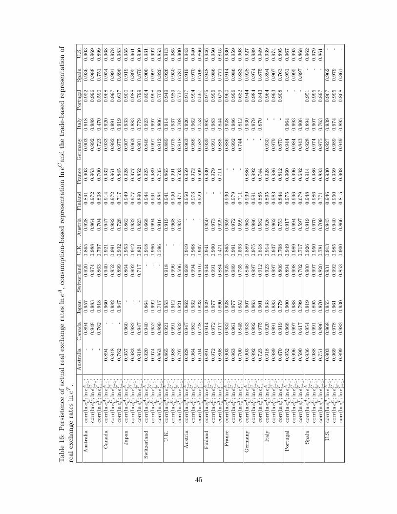
Tab

le16

:Per

sist

ence

ofac

tual

real

exch

ange

rate

sln

eA,c

onsu

mpt

ion-

base

dre

pres

enta

tion

lneC

and

the

trad

e-ba

sed

repr

esen

tati

onof

real

exch

ange

rate

sln

eT.

Aust

ralia

Canada

Japan

Sw

itze

rland

U.K

.A

ust

ria

Fin

land

Fra

nce

Ger

many

Italy

Port

ugal

Spain

U.S

.

Aust

ralia

corr

(ln

eA t;l

neA t+

1)

-0.8

94

0.9

57

0.9

20

0.8

65

0.9

28

0.8

91

0.9

03

0.9

03

0.9

18

0.9

52

0.9

36

0.9

03

corr

(ln

eC t;l

neC t+

1)

-0.9

48

0.9

83

0.9

74

0.9

88

0.9

64

0.9

72

0.9

63

0.9

92

0.9

89

0.9

96

0.9

88

0.9

69

corr

(ln

eT t;l

neT t+

1)

-0.7

62

0.9

18

0.8

63

0.7

97

0.7

04

0.8

08

0.7

00

0.7

23

0.4

70

0.5

90

0.7

51

0.8

99

Canada

corr

(ln

eA t;l

neA t+

1)

0.8

94

-0.9

60

0.9

40

0.9

21

0.9

47

0.9

14

0.9

32

0.9

33

0.9

20

0.9

68

0.9

54

0.9

68

corr

(ln

eC t;l

neC t+

1)

0.9

48

-0.9

82

0.9

52

0.9

91

0.9

82

0.9

72

0.9

61

0.9

92

0.9

91

0.9

97

0.9

91

0.9

78

corr

(ln

eT t;l

neT t+

1)

0.7

62

-0.9

47

0.8

99

0.9

32

0.7

28

0.7

17

0.8

45

0.9

75

0.9

19

0.6

17

0.8

96

0.9

83

Japan

corr

(ln

eA t;l

neA t+

1)

0.9

57

0.9

60

-0.8

64

0.9

53

0.8

62

0.9

49

0.9

28

0.9

07

0.9

33

0.9

00

0.9

19

0.9

55

corr

(ln

eC t;l

neC t+

1)

0.9

83

0.9

82

-0.9

92

0.9

12

0.9

32

0.9

77

0.9

77

0.9

63

0.8

83

0.9

88

0.8

95

0.9

61

corr

(ln

eT t;l

neT t+

1)

0.9

18

0.9

47

-0.7

17

0.8

21

0.8

23

0.8

90

0.8

52

0.9

01

0.7

79

0.7

99

0.8

70

0.9

30

Sw

itze

rland

corr

(ln

eA t;l

neA t+

1)

0.9

20

0.9

40

0.8

64

-0.9

18

0.6

68

0.9

44

0.9

25

0.8

46

0.9

23

0.8

94

0.9

00

0.9

31

corr

(ln

eC t;l

neC t+

1)

0.9

74

0.9

52

0.9

92

-0.9

96

0.9

94

0.9

91

0.9

89

0.9

97

0.9

97

0.9

98

0.9

97

0.9

92

corr

(ln

eT t;l

neT t+

1)

0.8

63

0.8

99

0.7

17

-0.5

96

0.9

16

0.8

84

0.7

35

0.9

12

0.8

06

0.7

02

0.8

20

0.8

53

U.K

.co

rr(l

neA t

;ln

eA t+1)

0.8

65

0.9

21

0.9

53

0.9

18

-0.9

19

0.9

41

0.8

65

0.8

89

0.9

14

0.9

49

0.9

26

0.9

13

corr

(ln

eC t;l

neC t+

1)

0.9

88

0.9

91

0.9

12

0.9

96

-0.9

68

0.9

90

0.9

91

0.9

75

0.9

37

0.9

89

0.9

50

0.9

85

corr

(ln

eT t;l

neT t+

1)

0.7

97

0.9

32

0.8

21

0.5

96

-0.9

37

0.4

71

0.5

93

0.8

18

0.7

08

0.7

17

0.7

81

0.9

00

Aust

ria

corr

(ln

eA t;l

neA t+

1)

0.9

28

0.9

47

0.8

62

0.6

68

0.9

19

-0.9

50

0.9

59

0.9

63

0.9

26

0.9

17

0.9

19

0.9

43

corr

(ln

eC t;l

neC t+

1)

0.9

64

0.9

82

0.9

32

0.9

94

0.9

68

-0.9

73

0.9

72

0.9

86

0.9

62

0.9

94

0.9

70

0.9

40

corr

(ln

eT t;l

neT t+

1)

0.7

04

0.7

28

0.8

23

0.9

16

0.9

37

-0.9

29

0.5

99

0.5

82

0.7

53

0.5

97

0.7

09

0.8

66

Fin

land

corr

(ln

eA t;l

neA t+

1)

0.8

91

0.9

14

0.9

49

0.9

44

0.9

41

0.9

50

-0.9

30

0.9

39

0.8

95

0.9

75

0.9

48

0.9

46

corr

(ln

eC t;l

neC t+

1)

0.9

72

0.9

72

0.9

77

0.9

91

0.9

90

0.9

73

-0.9

79

0.9

91

0.9

83

0.9

96

0.9

86

0.9

50

corr

(ln

eT t;l

neT t+

1)

0.8

08

0.7

17

0.8

90

0.8

84

0.4

71

0.9

29

-0.7

11

0.8

85

0.8

44

0.6

79

0.7

71

0.8

15

Fra

nce

corr

(ln

eA t;l

neA t+

1)

0.9

03

0.9

32

0.9

28

0.9

25

0.8

65

0.9

59

0.9

30

-0.8

86

0.9

28

0.9

60

0.9

14

0.9

30

corr

(ln

eC t;l

neC t+

1)

0.9

63

0.9

61

0.9

77

0.9

89

0.9

91

0.9

72

0.9

79

-0.9

92

0.9

86

0.9

96

0.9

86

0.9

59

corr

(ln

eT t;l

neT t+

1)

0.7

00

0.8

45

0.8

52

0.7

35

0.5

93

0.5

99

0.7

11

-0.7

44

0.8

12

0.6

82

0.8

83

0.9

08

Ger

many

corr

(ln

eA t;l

neA t+

1)

0.9

03

0.9

33

0.9

07

0.8

46

0.8

89

0.9

63

0.9

39

0.8

86

-0.9

30

0.9

44

0.9

28

0.9

27

corr

(ln

eC t;l

neC t+

1)

0.9

92

0.9

92

0.9

63

0.9

97

0.9

75

0.9

86

0.9

91

0.9

92

-0.9

79

0.9

84

0.9

74

0.9

89

corr

(ln

eT t;l

neT t+

1)

0.7

23

0.9

75

0.9

01

0.9

12

0.8

18

0.5

82

0.8

85

0.7

44

-0.8

70

0.8

43

0.8

75

0.9

49

Italy

corr

(ln

eA t;l

neA t+

1)

0.9

18

0.9

20

0.9

33

0.9

23

0.9

14

0.9

26

0.8

95

0.9

28

0.9

30

-0.9

64

0.8

94

0.9

39

corr

(ln

eC t;l

neC t+

1)

0.9

89

0.9

91

0.8

83

0.9

97

0.9

37

0.9

62

0.9

83

0.9

86

0.9

79

-0.9

93

0.9

07

0.9

74

corr

(ln

eT t;l

neT t+

1)

0.4

70

0.9

19

0.7

79

0.8

06

0.7

08

0.7

53

0.8

44

0.8

12

0.8

70

-0.9

08

0.7

63

0.8

95

Port

ugal

corr

(ln

eA t;l

neA t+

1)

0.9

52

0.9

68

0.9

00

0.8

94

0.9

49

0.9

17

0.9

75

0.9

60

0.9

44

0.9

64

-0.9

51

0.9

67

corr

(ln

eC t;l

neC t+

1)

0.9

96

0.9

97

0.9

88

0.9

98

0.9

89

0.9

94

0.9

96

0.9

96

0.9

84

0.9

93

-0.9

95

0.9

95

corr

(ln

eT t;l

neT t+

1)

0.5

90

0.6

17

0.7

99

0.7

02

0.7

17

0.5

97

0.6

79

0.6

82

0.8

43

0.9

08

-0.8

97

0.8

68

Spain

corr

(ln

eA t;l

neA t+

1)

0.9

36

0.9

54

0.9

19

0.9

00

0.9

26

0.9

19

0.9

48

0.9

14

0.9

28

0.8

94

0.9

51

-0.9

62

corr

(ln

eC t;l

neC t+

1)

0.9

88

0.9

91

0.8

95

0.9

97

0.9

50

0.9

70

0.9

86

0.9

86

0.9

74

0.9

07

0.9

95

-0.9

79

corr

(ln

eT t;l

neT t+

1)

0.7

51

0.8

96

0.8

70

0.8

20

0.7

81

0.7

09

0.7

71

0.8

83

0.8

75

0.7

63

0.8

97

-0.8

61

U.S

.co

rr(l

neA t

;ln

eA t+1)

0.9

03

0.9

68

0.9

55

0.9

31

0.9

13

0.9

43

0.9

46

0.9

30

0.9

27

0.9

39

0.9

67

0.9

62

-

corr

(ln

eC t;l

neC t+

1)

0.9

69

0.9

78

0.9

61

0.9

92

0.9

85

0.9

40

0.9

50

0.9

59

0.9

89

0.9

74

0.9

95

0.9

79

-

corr

(ln

eT t;l

neT t+

1)

0.8

99

0.9

83

0.9

30

0.8

53

0.9

00

0.8

66

0.8

15

0.9

08

0.9

49

0.8

95

0.8

68

0.8

61

-

45

Tab

le17

:C

orre

lati

onof

rela

tive

cons

umpt

ions

wit

hac

tual

real

exch

ange

rate

s,co

nsum

ptio

n-ba

sed

repr

esen

tati

onln

eCan

dth

etr

ade-

base

dre

pres

enta

tion

ofre

alex

chan

gera

tes

lneT

.A

ust

ralia

Canada

Japan

Sw

itze

rland

U.K

.A

ust

ria

Fin

land

Fra

nce

Ger

many

Italy

Port

ugal

Spain

U.S

.

Aust

ralia

corr

(ln

eA;l

nci

/cj

)-

-0.2

62

-0.7

58

0.5

87

-0.4

81

-0.6

86

-0.6

87

-0.3

07

-0.6

78

-0.7

08

-0.8

36

-0.7

67

-0.2

25

corr

(ln

eC;l

nci

/cj

)-

11

11

11

11

11

11

corr

(ln

eT;l

nci

/cj

)-

-0.2

57

-0.7

79

0.4

62

-0.4

63

0.5

09

-0.5

77

0.0

88

0.0

88

-0.3

17

0.5

87

0.1

22

0.3

75

Canada

corr

(ln

eA;l

nci

/cj

)-0

.262

--0

.712

0.5

24

-0.4

44

-0.5

64

-0.2

55

-0.2

85

-0.6

52

-0.6

81

-0.8

43

-0.7

01

-0.3

67

corr

(ln

eC;l

nci

/cj

)1

-1

11

11

11

11

11

corr

(ln

eT;l

nci

/cj

)-0

.257

--0

.632

0.6

35

-0.4

07

-0.5

45

0.1

03

-0.1

14

-0.7

31

-0.6

06

-0.0

53

-0.7

86

-0.6

45

Japan

corr

(ln

eA;l

nci

/cj

)-0

.758

-0.7

12

--0

.473

0.2

45

-0.4

82

-0.7

41

-0.5

72

0.0

90

-0.2

72

-0.1

73

-0.5

00

-0.6

51

corr

(ln

eC;l

nci

/cj

)1

1-

11

11

11

11

11

corr

(ln

eT;l

nci

/cj

)-0

.779

-0.6

32

--0

.439

0.2

22

-0.5

09

-0.7

74

-0.6

97

0.2

02

-0.3

56

-0.0

33

-0.0

41

-0.7

72

Sw

itze

rland

corr

(ln

eA;l

nci

/cj

)0.5

87

0.5

24

-0.4

73

-0.5

86

0.0

71

0.3

16

0.7

08

0.5

67

0.3

69

-0.5

89

0.0

38

0.6

01

corr

(ln

eC;l

nci

/cj

)1

11

-1

11

11

11

11

corr

(ln

eT;l

nci

/cj

)0.4

62

0.6

35

-0.4

39

-0.2

84

0.8

88

0.6

02

0.3

40

0.8

79

0.3

70

0.6

98

0.3

67

0.4

78

U.K

.co

rr(l

neA

;ln

ci/cj

)-0

.481

-0.4

44

0.2

45

0.5

86

-0.6

35

-0.3

09

0.1

22

-0.1

09

0.3

70

-0.7

47

0.3

12

-0.4

31

corr

(ln

eC;l

nci

/cj

)1

11

1-

11

11

11

11

corr

(ln

eT;l

nci

/cj

)-0

.463

-0.4

07

0.2

22

0.2

84

-0.5

28

-0.1

20

-0.3

48

0.0

17

0.1

64

-0.3

94

0.1

83

-0.7

65

Aust

ria

corr

(ln

eA;l

nci

/cj

)-0

.686

-0.5

64

-0.4

82

0.0

71

0.6

35

--0

.761

-0.4

13

0.5

51

0.2

28

-0.6

28

-0.3

22

-0.0

77

corr

(ln

eC;l

nci

/cj

)1

11

11

-1

11

11

11

corr

(ln

eT;l

nci

/cj

)0.5

09

-0.5

45

-0.5

09

0.8

88

0.5

28

--0

.438

-0.0

95

-0.2

05

-0.0

09

0.2

20

0.3

71

-0.3

55

Fin

land

corr

(ln

eA;l

nci

/cj

)-0

.687

-0.2

55

-0.7

41

0.3

16

-0.3

09

-0.7

61

--0

.326

-0.8

01

-0.4

99

-0.8

54

-0.8

70

-0.2

95

corr

(ln

eC;l

nci

/cj

)1

11

11

1-

11

11

11

corr

(ln

eT;l

nci

/cj

)-0

.577

0.1

03

-0.7

74

0.6

02

-0.1

20

-0.4

38

--0

.293

-0.7

03

-0.7

37

-0.7

38

-0.7

34

-0.3

11

Fra

nce

corr

(ln

eA;l

nci

/cj

)-0

.307

-0.2

85

-0.5

72

0.7

08

0.1

22

-0.4

13

-0.3

26

--0

.445

0.0

87

-0.8

81

-0.2

99

-0.0

73

corr

(ln

eC;l

nci

/cj

)1

11

11

11

-1

11

11

corr

(ln

eT;l

nci

/cj

)0.0

88

-0.1

14

-0.6

97

0.3

40

-0.3

48

-0.0

95

-0.2

93

-0.4

12

0.4

18

-0.1

94

-0.3

64

-0.1

86

Ger

many

corr

(ln

eA;l

nci

/cj

)-0

.678

-0.6

52

0.0

90

0.5

67

-0.1

09

0.5

51

-0.8

01

-0.4

45

--0

.566

-0.6

14

-0.1

30

-0.5

26

corr

(ln

eC;l

nci

/cj

)1

11

11

11

1-

11

11

corr

(ln

eT;l

nci

/cj

)0.0

88

-0.7

31

0.2

02

0.8

79

0.0

17

-0.2

05

-0.7

03

0.4

12

--0

.420

0.3

66

-0.3

82

-0.6

17

Italy

corr

(ln

eA;l

nci

/cj

)-0

.708

-0.6

81

-0.2

72

0.3

69

0.3

70

0.2

28

-0.4

99

0.0

87

-0.5

66

--0

.700

-0.0

52

-0.5

55

corr

(ln

eC;l

nci

/cj

)1

11

11

11

11

-1

11

corr

(ln

eT;l

nci

/cj

)-0

.317

-0.6

06

-0.3

56

0.3

70

0.1

64

-0.0

09

-0.7

37

0.4

18

-0.4

20

--0

.759

0.2

02

-0.4

00

Port

ugal

corr

(ln

eA;l

nci

/cj

)-0

.836

-0.8

43

-0.1

73

-0.5

89

-0.7

47

-0.6

28

-0.8

54

-0.8

81

-0.6

14

-0.7

00

--0

.558

-0.8

60

corr

(ln

eC;l

nci

/cj

)1

11

11

11

11

1-

11

corr

(ln

eT;l

nci

/cj

)0.5

87

-0.0

53

-0.0

33

0.6

98

-0.3

94

0.2

20

-0.7

38

-0.1

94

0.3

66

-0.7

59

-0.3

15

0.3

14

Spain

corr

(ln

eA;l

nci

/cj

)-0

.767

-0.7

01

-0.5

00

0.0

38

0.3

12

-0.3

22

-0.8

70

-0.2

99

-0.1

30

-0.0

52

-0.5

58

--0

.595

corr

(ln

eC;l

nci

/cj

)1

11

11

11

11

11

-1

corr

(ln

eT;l

nci

/cj

)0.1

22

-0.7

86

-0.0

41

0.3

67

0.1

83

0.3

71

-0.7

34

-0.3

64

-0.3

82

0.2

02

0.3

15

--0

.639

U.S

.co

rr(l

neA

;ln

ci/cj

)-0

.225

-0.3

67

-0.6

51

0.6

01

-0.4

31

-0.0

77

-0.2

95

-0.0

73

-0.5

26

-0.5

55

-0.8

60

-0.5

95

-co

rr(l

neC

;ln

ci/cj

)1

11

11

11

11

11

1-

corr

(ln

eT;l

nci

/cj

)0.3

75

-0.6

45

-0.7

72

0.4

78

-0.7

65

-0.3

55

-0.3

11

-0.1

86

-0.6

17

-0.4

00

0.3

14

-0.6

39

-

46

References

Alvarez, Fernando and Urban J. Jermann, “Efficiency, Equilibrium and Asset Pricing with Risk ofDefault,” Econometrica, Jul 2000, 68 (4), 775–797.

and , “Quantitative Asset Pricing Implications of Endogenous Solvency Constraints,” Review ofFinancial Studies, Winter 2001, 14 (4), 1117–1151.

Atkeson, Andrew and Ariel Burstein, “International Relative Prices in New Ricardian Models of In-ternational Trade,” Working Paper, 2004.

Backus, David K. and Gregor W. Smith, “Consumption and Real Exchange Rates in DynamicEconomies with Non-traded goods,” Journal of International Economics, Nov 1993, 35 (3-4), 297–316.

, Patrick J. Kehoe, and Finn E. Kydland, “International Real Business Cycles,” Journal ofPolitical Economy, Aug 1992, 100 (4), 745–775.

, , and , “Dynamics of the Trade Balance and the Terms of Trade: The J-Curve?,” AmericanEconomic Review, Mar 1994, 84 (1), 84–103.

Balassa, Bela, “The Purchasing-Power Parity Doctrine: A Reappraisal,” Journal of Political Economy,Dec 1964, 72 (6), 584–596.

Baltagi, Badi H., “Econometric Analysis of Panel Data,” John Wiley and Sons Ltd, 2001, 2nd Edition.

and Chihwa Kao, “Nonstationary Panels,Cointegration in Panels and Dynamic Panels: A Survey,”Advances in Econometrics, 2000, 15, 7–51.

Baxter, Marianne and Robert G. King, “Measuring Business Cycles: Approximate Band-Pass Filtersfor Economic Time Series,” Review of Economics and Statistics, Nov 1999, 81 (4), 575–593.

, Urban J. Jermann, and Robert G. King, “Nontraded Goods, Nontraded Factors and Interna-tional Non-Diversification,” Journal of International Economics, Apr 1998, 44 (2), 211–229.

Betts, Caroline and Michael B. Devereux, “Exchange Rate Dynamics in a Model of Pricing-to-Market,”Journal of International Economics, Feb 2000, 50 (1), 215–244.

Betts, Caroline M. and Timothy J. Kehoe, “U.S. Real Exchange Rate Fluctuations and Relative PriceFluctuations,” Federal Reserve Bank of Minneapolis, Research Department Staff Report 334, 2004.

Brandt, Michael W., John H. Cochrane, and Pedro Santa-Clara, “International Risk Sharing isBetter than You Think (Or Exchange Rates are Much Too Smooth),” Working Paper, 2004.

Canova, Fabio and Morten O. Ravn, “International Consumption Risk Sharing,” International Eco-nomic Review, Aug 1996, 37 (3), 573–601.

Chari, V.V., Patrick J. Kehoe, and Ellen R. McGrattan, “Can Sticky Price Models Generate Volatileand Persistent Real Exchange Rates?,” Review of Economic Studies, Jul 2002, 69 (3), 533–563.

Chinn, Menzie D. and Richard A. Meese, “Banking on Currency Forecasts - How Predictable is Changein Money,” Journal of International Economics, Feb 1995, 38 (1-2), 161–178.

Corsetti, Giancarlo, Luca Dedola, and Sylvain Leduc, “Consumption and Real Exchange Rates withGoods and Asset Market Frictions,” Working Paper, 2002.

47

Davidson, Russell and James G. MacKinnon, “Estimation and Inference in Econometrics,” OxfordUniversity Press, 1993.

Devereux, Michael, “Real Exchange Rates and Macroeconomics: Evidence and Theory,” Canadian Jour-nal of Economics, Nov 1997, pp. 773–808.

Dickey, David A. and Wayne A. Fuller, “Distribution of the Estimators for Autoregressive Time SeriesWith a Unit Root,” Journal of American Statistical Association, Jun 79, 74 (366), 427–431.

Dornbusch, Rudiger, “Expectations and Exchange Rates Dynamics,” Journal of Political Economy, De-cember 1976, 84 (6), 1161–76.

Dumas, Bernard, “Dynamic Equilibrium and the Real Exchange Rate in a Spatially Separated World,”Review of Financial Studies, 1992, 5 (2), 153–180.

Eaton, Jonathan and Mark Gersovitz, “Debt with Potential Repudiation: Theoretical and EmpiricalAnalysis,” Review of Economic Studies, Apr 1981, 48 (2), 289–309.

and Samuel Kortum, “Technology, Geography and Trade,” Econometrica, Sep 2002, 70 (5), 1741–1779.

Engel, Charles, “Accounting for U.S. Real Exchange Rate Changes,” Journal of Political Economy, Jun1999, 107 (3), 507–538.

and Kenneth D. West, “Accounting for Exchange-Rate Variability in Present-Value Models Whenthe Discount Factor Is Near 1,” American Economic Review, May 2004, 94 (2), 119–125.

and , “Exchange Rates and Fundamentals,” Working Paper, 2004.

Fitzgerald, Doireann, “Trade, Interdependence and Exchange Rates,” Working Paper, 2004.

Frankel, Jeffrey A. and Andrew K. Rose, “A Panel Project on Purchasing Power Parity Mean Reversionwithin and between Countries,” Journal of International Economics, 1996, 40, 209–224.

and Andrew Rose, “A Survey of Empirical Research on Nominal Exchange Rates,” Handbook ofInternational Economics, 1995, 3.

Heathcote, Jonathan and Fabrizio Perri, “The International Diversification Puzzle is not as Bad asYou Think,” Working Paper, 2004.

Kao, Chihwa, “Spurious Regression and Residual-based Tests for Cointegration in Panel Data,” Journalof Econometrics, 1999, 90, 1–44.

Kehoe, Patrick J. and Fabrizio Perri, “International Real Business Cycles with Endogenous IncompleteMarkets,” Econometrica, May 2002, 70 (3), 907–928.

Kehoe, Timothy and David Levine, “Debt-Constrained Asset Markets,” Review of Economic Studies,Oct 1993, 60 (4), 865–888.

Kocherlakota, Narayana, “Implications of Efficient Risk Sharing Without Commitment,” Review of Eco-nomic Studies, Oct 1996, 63 (4), 595–609.

Kollman, Robert, “Consumption, Real Exchange Rates and the Structure of International Asset Markets,”Journal of International Money and Finance, 1995, 14 (2), 191–211.

48

Levin, Andrew and Chien-Fu Lin, “Unit Root Test in Panel Data: New Results,” Discussion Paper No.93-56 (University of California at San Diego), 1993.

, , and Chia-Shang James Chu, “Unit Roots in Panel Data Asymptotic and Finite SampleProperties,” Journal of Econometrics, May 2002, 108 (1), 1–14.

Lucas, Robert, “Interest Rates and Currency Prices in a Two-Country World,” Journal of MonetaryEconomics, 1983, 10 (3), 335–359.

MacKinnon, James, “Critical Values in Cointegration Tests,” Long Run Economic Relationships: Readingsin Cointegration, edited by R.F. Engle and C.W.J Granger, 1991, pp. 267–276.

Meese, Richard A. and Kenneth Rogoff, “Empirical Exchange Rate Models of the Seventies: Do theyFit Out of Sample?,” Journal of International Economics, 1983, 14 (1-2), 3–24.

Newey, Whitney K. and Kenneth D. West, “Simple Positive Semi-Definite Heteroscedasticity andAutocorrelation Consistent Covariance Matrix,” Econometrica, May 1987, 55 (3), 703–708.

Obstfeld, Maurice and Kenneth Rogoff, “Exchange Rate Dynamics Redux,” Journal of Political Econ-omy, Jun 1995, 103 (3), 624–660.

and , “Foundations of International Macroeconomics,” MIT Press, 1996.

and , “The Six Major Puzzles in International Macroeconomics: Is there a Common Cause?,”NBER Macroeconomics Annual, 2000, 15, 339–390.

Pavlova, Anna and Roberto Rigobon, “Asset Prices and Exchange Rates,” Working Paper, 2004.

Phillips, Peter C. B. and Pierre Perron, “Testing for a Unit Root in Time Series Regression,”Biometrika, 1988, 75 (2), 335–346.

Rajan, Priya and Jae Young Lee, “Contract Enforcement and the Volume of International Trade inDifferent Types of Goods,” Working Paper, 2003.

Ravn, Morten O., “Consumption Dynamics and Real Exchange Rates,” Working Paper, 2004.

Rogoff, Kenneth, “The Purchasing Power Parity Puzzle,” Journal of Economic Literature, June 1996,XXXIV, 647–668.

Samuelson, Paul A., “Theoretical Notes on Trade Problems,” The Review of Economics and Statistics,May 1964, 46 (2), 145–154.

Sercu, Piet and Raman Uppal, “Exchange Rate Volatility and International Trade: A General-Equilibrium Analysis,” European Economic Review, Jun 2003, 3 (3), 429–441.

Stockman, Alan and Linda Tesar, “Tastes and Technology in a Two Country Model of the BusinessCycle: Explaining International Comovements,” NBER Working Paper 3566, 1990.

and , “Tastes and Technology in a Two Country Model of the Business Cycle: ExplainingInternational Comovements,” American Economic Review, Mar 1995, 85 (1), 168–185.

Taylor, Alan, “Potential Pitfalls for the Purchasing-power-parity Puzzle? Sampling and SpecificationBiases in Mean-reversion Tests of the Law of One Price,” Econometrica, Mar 2001, 69 (2), 473–498.

Uppal, Rama, “A General Equilibrium Model of International Portfolio Choice,” Journal of Finance, Jun1993, 48 (2), 529–553.

49

Real Exchange Rates, International Trade and Macroeconomic

Documents

Transcript of Real Exchange Rates, International Trade and Macroeconomic