Re-examining the influence of work and non-work accessibility on residential location choices with a...

Re-examining the influence of

work and non-work accessibility on

residential location choices with

a micro-analytic framework

Brian H. Y. Lee

Dept. of Urban Design & Planning

University of Washington

1 May 2009

Transportation Seminars

Center for Transportation Studies

Portland State University

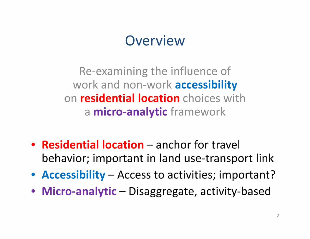
Overview

Re-examining the influence ofwork and non-work accessibility

on residential location choices with a micro-analytic framework

• Residential location – anchor for travel behavior; important in land use-transport link

• Accessibility – Access to activities; important?

• Micro-analytic – Disaggregate, activity-based

2

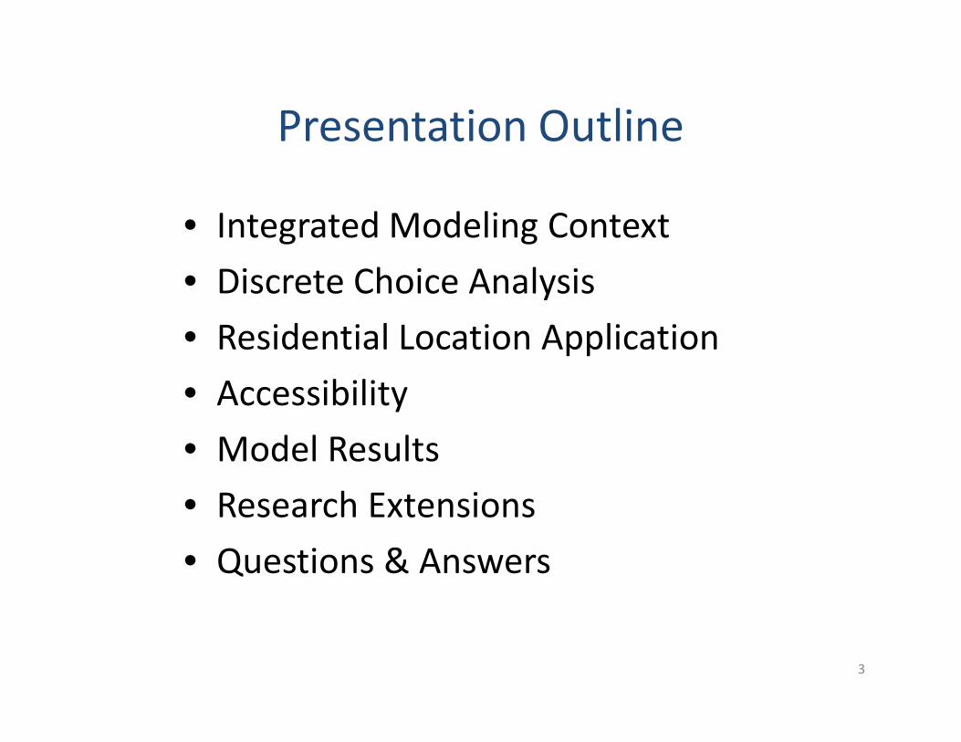
Presentation Outline

• Integrated Modeling Context

• Discrete Choice Analysis

• Residential Location Application

• Accessibility

• Model Results

• Research Extensions

• Questions & Answers

3

� Integrated

Modeling Context

Discrete Choice

Analysis

Residential Location

Application

Accessibility

Model Results

Research Extensions

Questions & Answers

4

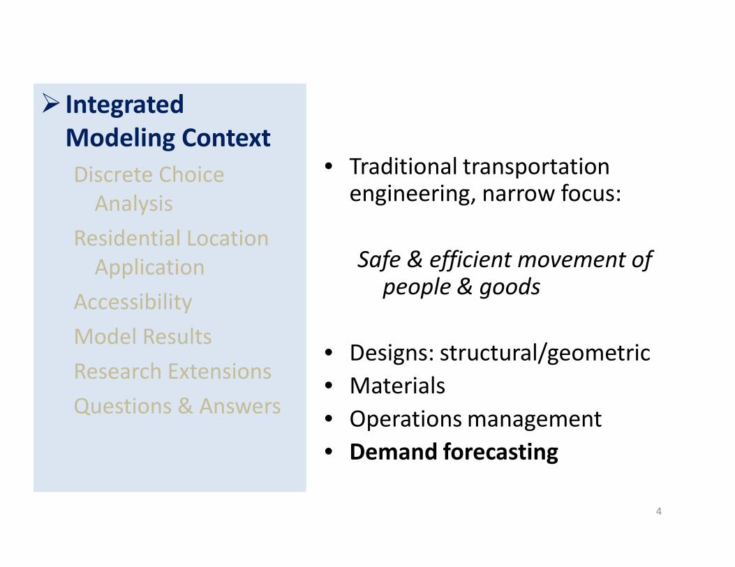
• Traditional transportation engineering, narrow focus:

Safe & efficient movement of

people & goods

• Designs: structural/geometric

• Materials

• Operations management

• Demand forecasting

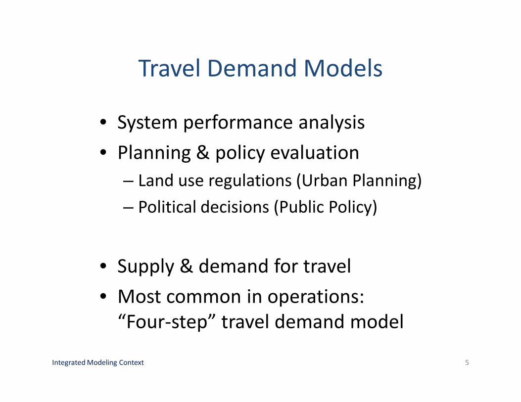
Travel Demand Models

• System performance analysis

• Planning & policy evaluation

– Land use regulations (Urban Planning)

– Political decisions (Public Policy)

• Supply & demand for travel

• Most common in operations:

“Four-step” travel demand model

Integrated Modeling Context 5

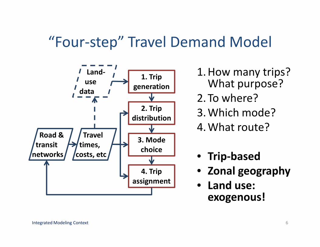
Travel

times,

costs, etc

Road &

transit

networks

“Four-step” Travel Demand Model

1. How many trips? What purpose?

2. To where?

3. Which mode?

4. What route?

• Trip-based

• Zonal geography

• Land use: exogenous!


1. Trip

generation

2. Trip

distribution

3. Mode

choice

4. Trip

assignment

Land-

use

data

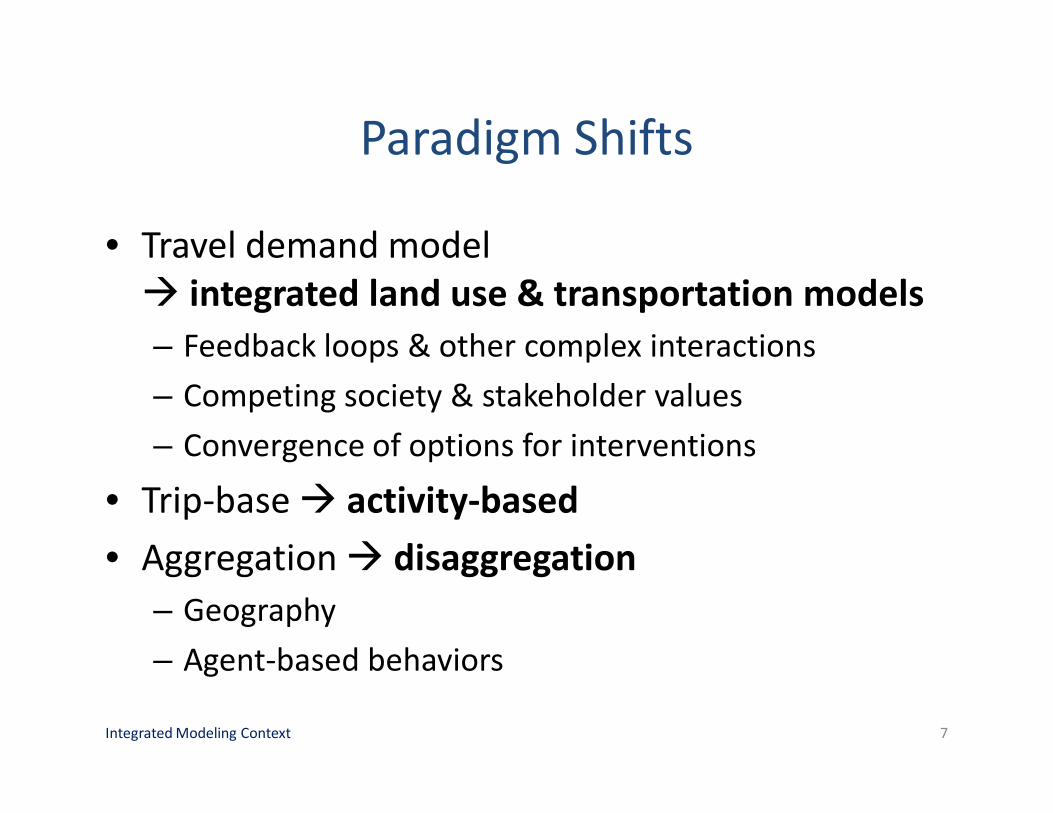
Paradigm Shifts

• Travel demand model

� integrated land use & transportation models

– Feedback loops & other complex interactions

– Competing society & stakeholder values

– Convergence of options for interventions

• Trip-base � activity-based

• Aggregation � disaggregation

– Geography

– Agent-based behaviors


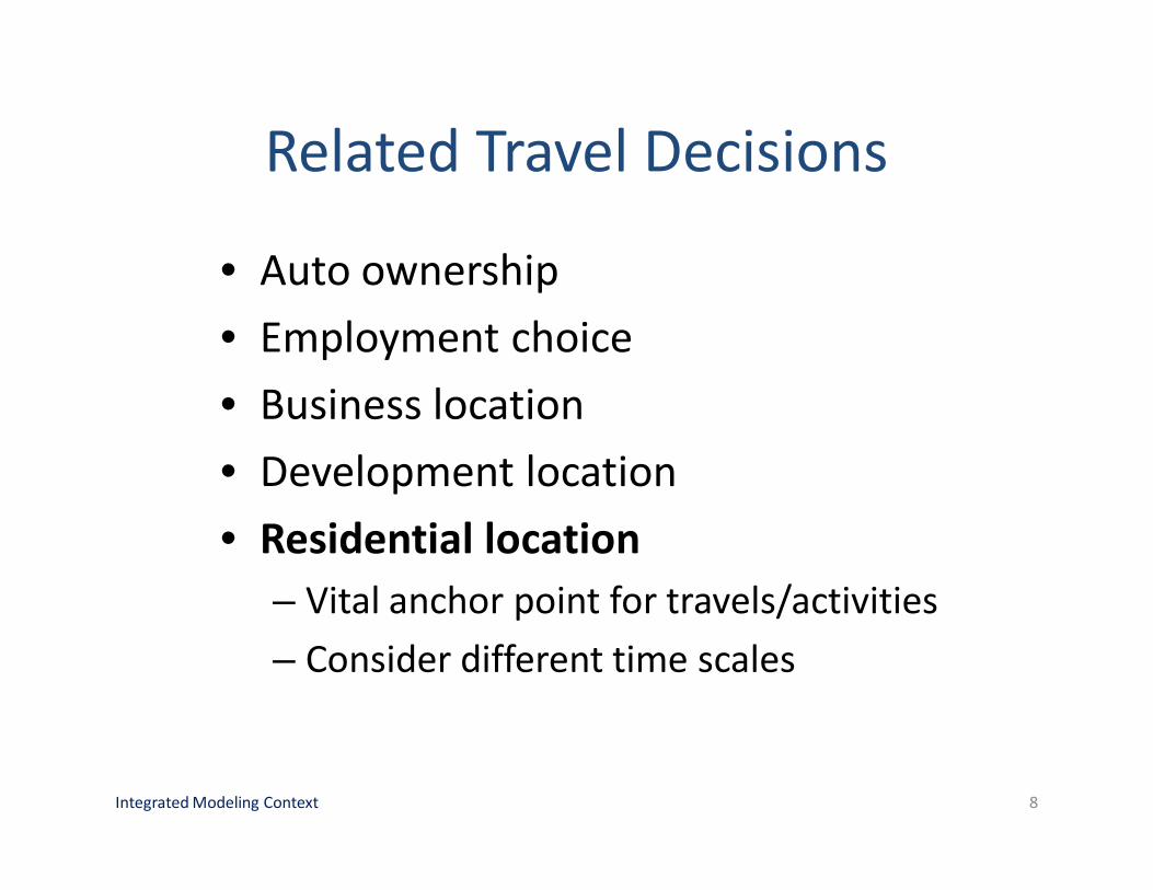
Related Travel Decisions

• Auto ownership

• Employment choice

• Business location

• Development location

• Residential location

– Vital anchor point for travels/activities

– Consider different time scales


Integrated Modeling

Context

�Discrete Choice

Analysis


Application

Accessibility

Model Results

Research Extensions

Questions & Answers

9

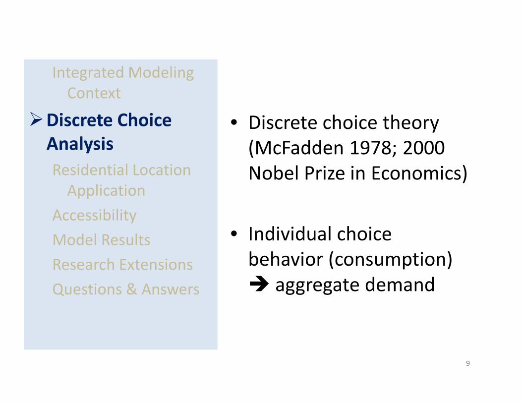
• Discrete choice theory

(McFadden 1978; 2000

Nobel Prize in Economics)

• Individual choice

behavior (consumption)

� aggregate demand

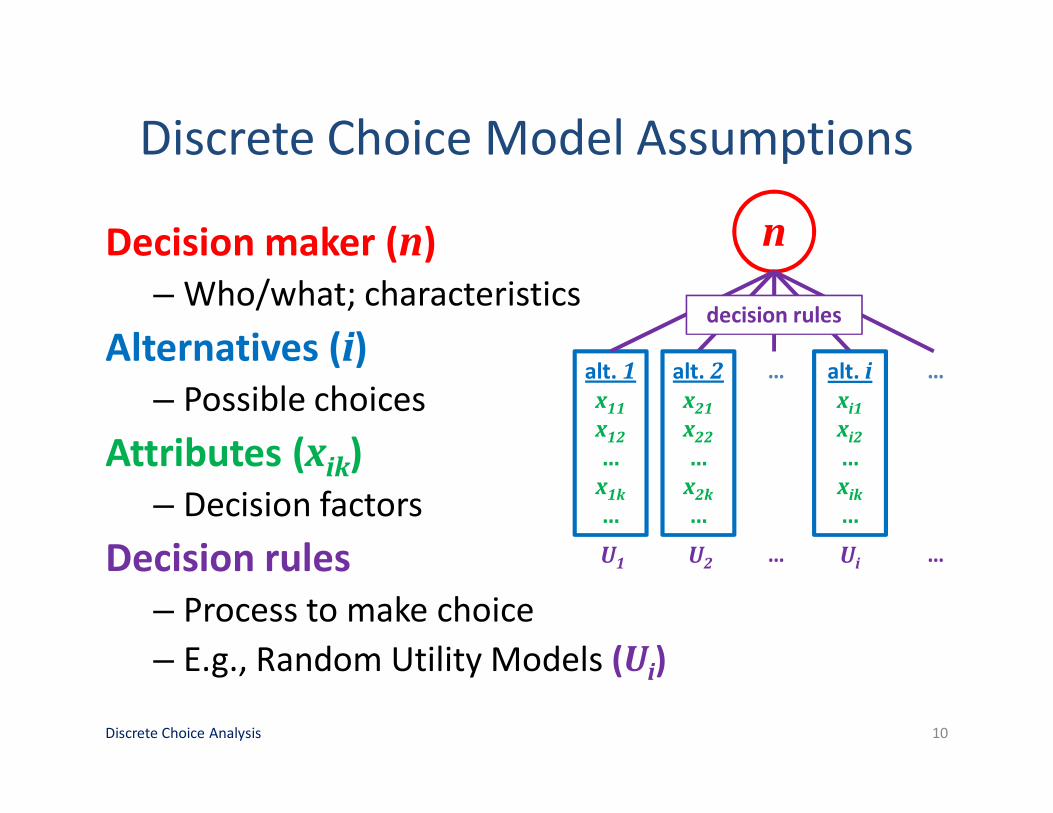
Discrete Choice Model Assumptions

Decision maker (n)

– Who/what; characteristics

Alternatives (i)

– Possible choices

Attributes (xik)

– Decision factors

Decision rules

– Process to make choice

– E.g., Random Utility Models (Ui)

Discrete Choice Analysis 10

n

alt. 1

x11

x12

…

x1k

…

… …

decision rules

alt. i

xi1

xi2

…

xik

…

alt. 2

x21

x22

…

x2k

…

U1 U2 Ui… …

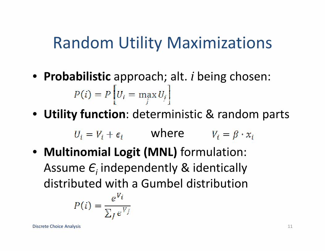
Random Utility Maximizations

• Probabilistic approach; alt. i being chosen:

• Utility function: deterministic & random parts

where

• Multinomial Logit (MNL) formulation:

Assume Єi independently & identically

distributed with a Gumbel distribution


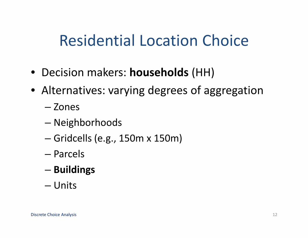
Residential Location Choice

• Decision makers: households (HH)

• Alternatives: varying degrees of aggregation

– Zones

– Neighborhoods

– Gridcells (e.g., 150m x 150m)

– Parcels

– Buildings

– Units


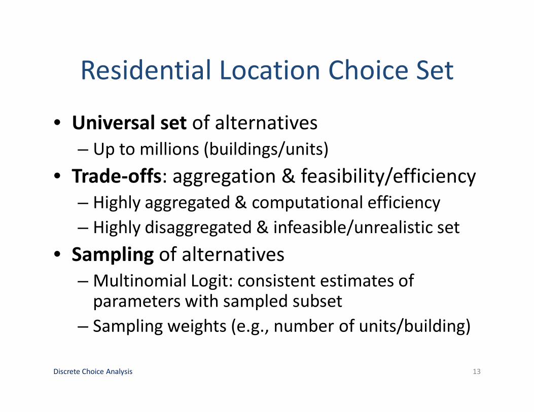
Residential Location Choice Set

• Universal set of alternatives

– Up to millions (buildings/units)

• Trade-offs: aggregation & feasibility/efficiency

– Highly aggregated & computational efficiency

– Highly disaggregated & infeasible/unrealistic set

• Sampling of alternatives

– Multinomial Logit: consistent estimates of parameters with sampled subset

– Sampling weights (e.g., number of units/building)


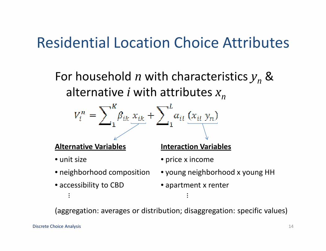
Residential Location Choice Attributes

For household n with characteristics yn &

alternative i with attributes xn


Alternative Variables Interaction Variables

• unit size • price x income

• neighborhood composition • young neighborhood x young HH

• accessibility to CBD • apartment x renter

… …

(aggregation: averages or distribution; disaggregation: specific values)

Integrated Modeling

Context

Discrete Choice

Analysis

�Residential Location

Application

Accessibility

Model Results

Research Extensions

Questions & Answers

15

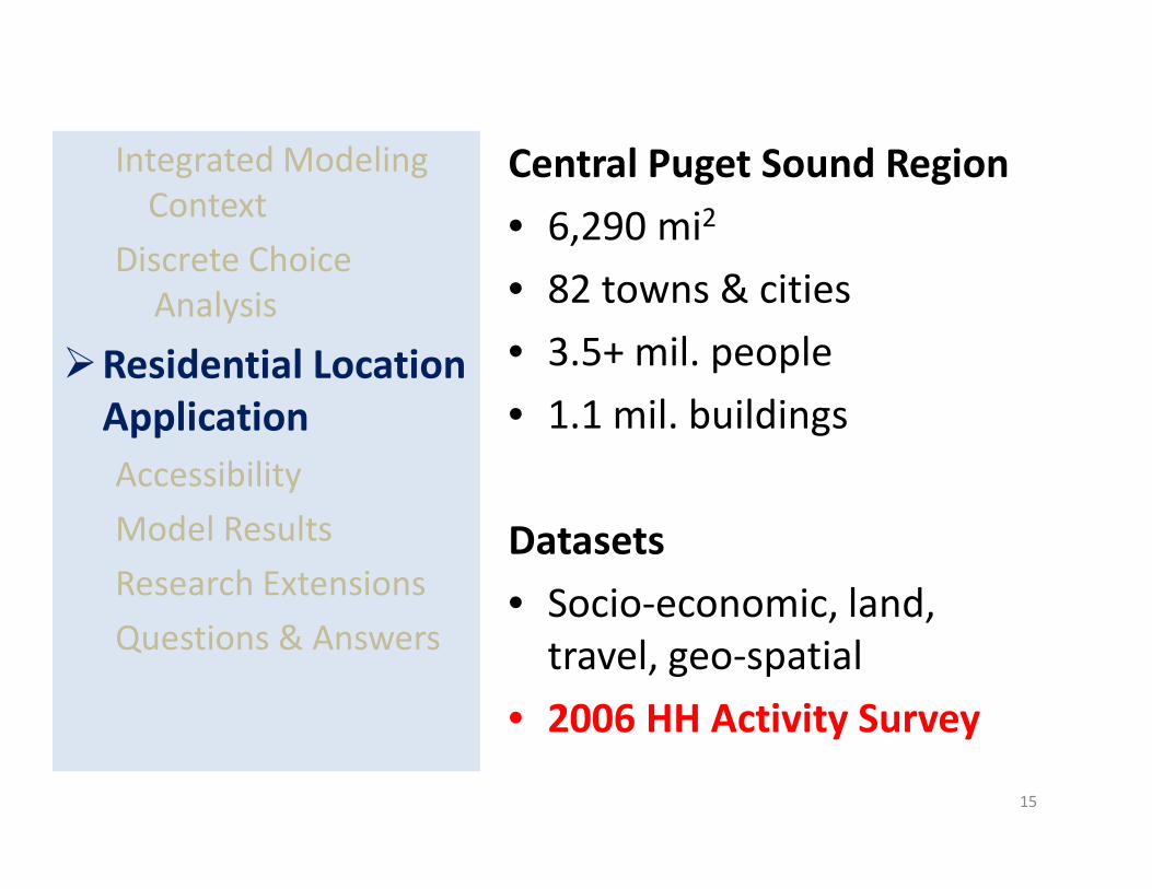
Central Puget Sound Region

• 6,290 mi2

• 82 towns & cities

• 3.5+ mil. people

• 1.1 mil. buildings

Datasets

• Socio-economic, land,

travel, geo-spatial

• 2006 HH Activity Survey

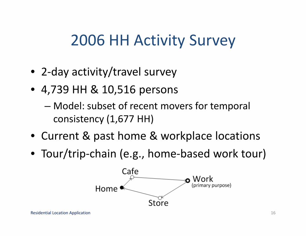
2006 HH Activity Survey

• 2-day activity/travel survey

• 4,739 HH & 10,516 persons

– Model: subset of recent movers for temporal

consistency (1,677 HH)

• Current & past home & workplace locations

• Tour/trip-chain (e.g., home-based work tour)

Residential Location Application 16

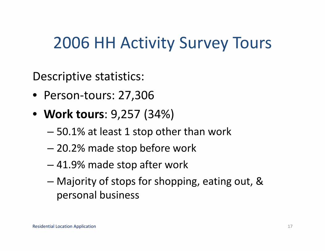
2006 HH Activity Survey Tours


Descriptive statistics:

• Person-tours: 27,306

• Work tours: 9,257 (34%)

– 50.1% at least 1 stop other than work

– 20.2% made stop before work

– 41.9% made stop after work

– Majority of stops for shopping, eating out, &

personal business

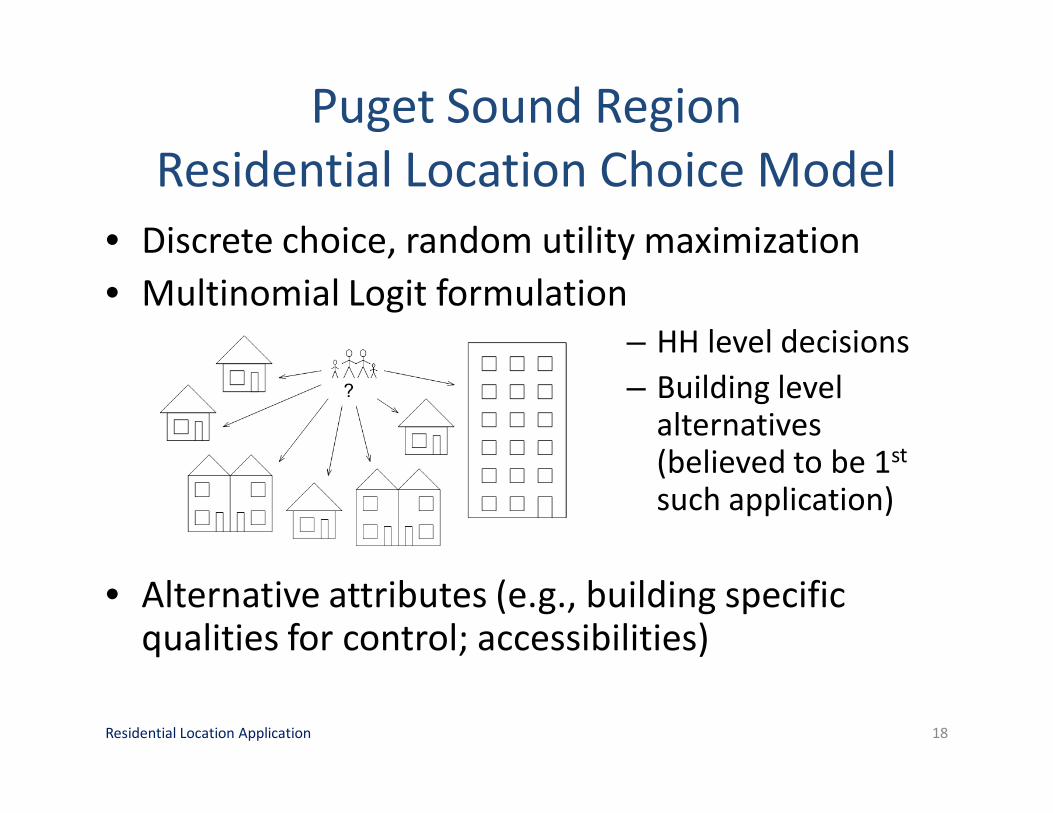
• Discrete choice, random utility maximization

• Multinomial Logit formulation

– HH level decisions

– Building levelalternatives(believed to be 1st

such application)

• Alternative attributes (e.g., building specific qualities for control; accessibilities)

Puget Sound Region

Residential Location Choice Model


Integrated Modeling

Context

Discrete Choice

Analysis


Application

�Accessibility

Model Results

Research Extensions

Questions & Answers

19

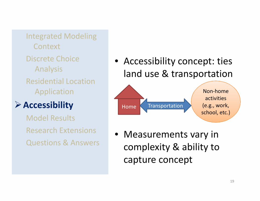
• Accessibility concept: ties

land use & transportation

• Measurements vary in

complexity & ability to

capture concept

Home

Non-home

activities

(e.g., work,

school, etc.)

Transportation

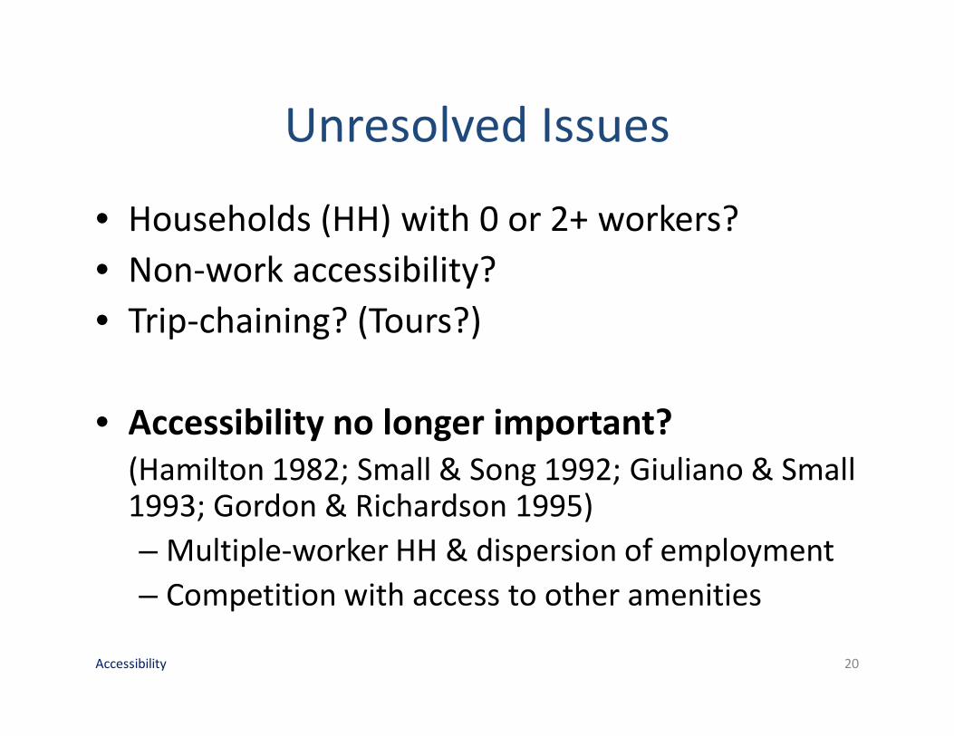
Unresolved Issues

• Households (HH) with 0 or 2+ workers?

• Non-work accessibility?

• Trip-chaining? (Tours?)

• Accessibility no longer important?

(Hamilton 1982; Small & Song 1992; Giuliano & Small 1993; Gordon & Richardson 1995)

– Multiple-worker HH & dispersion of employment

– Competition with access to other amenities

Accessibility 20

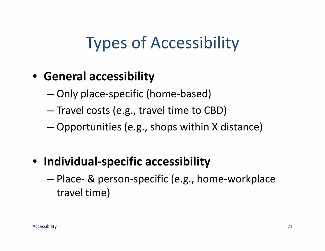
Types of Accessibility

• General accessibility

– Only place-specific (home-based)

– Travel costs (e.g., travel time to CBD)

– Opportunities (e.g., shops within X distance)

• Individual-specific accessibility

– Place- & person-specific (e.g., home-workplace

travel time)

Accessibility 21

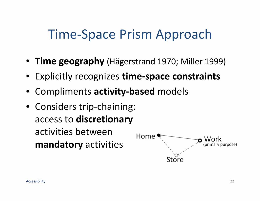
Time-Space Prism Approach

• Time geography (Hägerstrand 1970; Miller 1999)

• Explicitly recognizes time-space constraints

• Compliments activity-based models

• Considers trip-chaining:

access to discretionary

activities between

mandatory activities

Accessibility 22

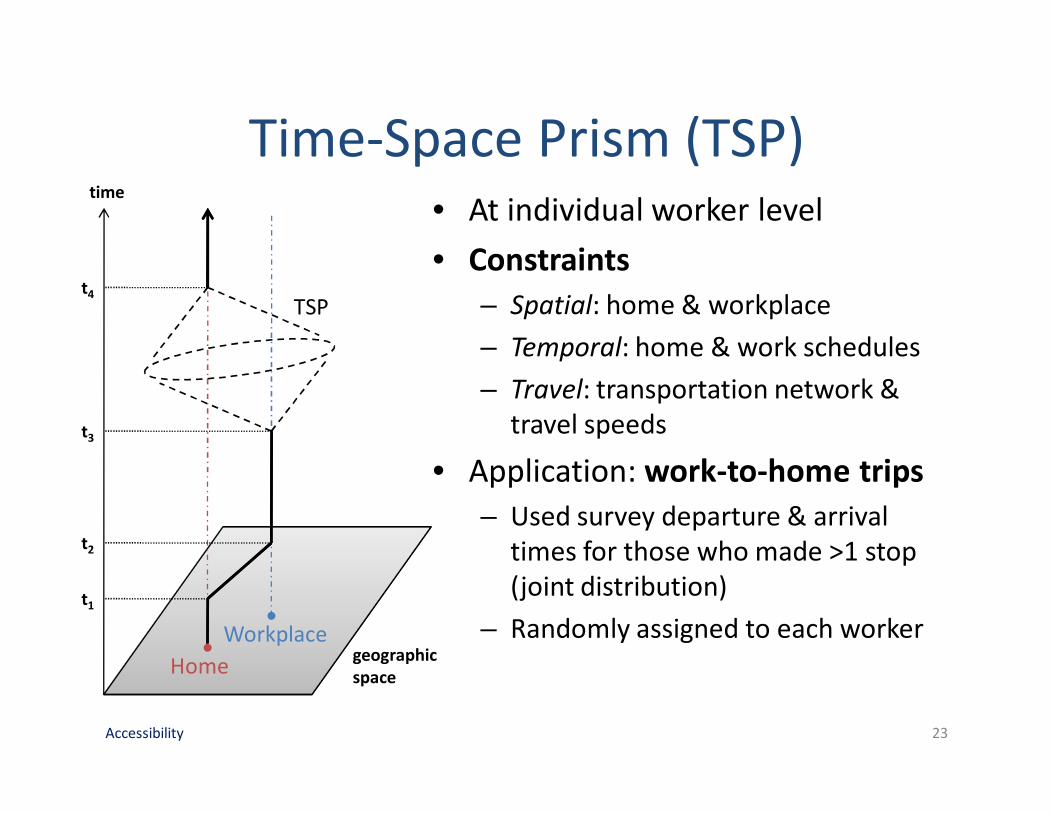
Time-Space Prism (TSP)• At individual worker level

• Constraints

– Spatial: home & workplace

– Temporal: home & work schedules

– Travel: transportation network &

travel speeds

• Application: work-to-home trips

– Used survey departure & arrival

times for those who made >1 stop

(joint distribution)

– Randomly assigned to each worker

Accessibility 23

time

Home

Workplacegeographic

space

TSP

t1

t2

t3

t4

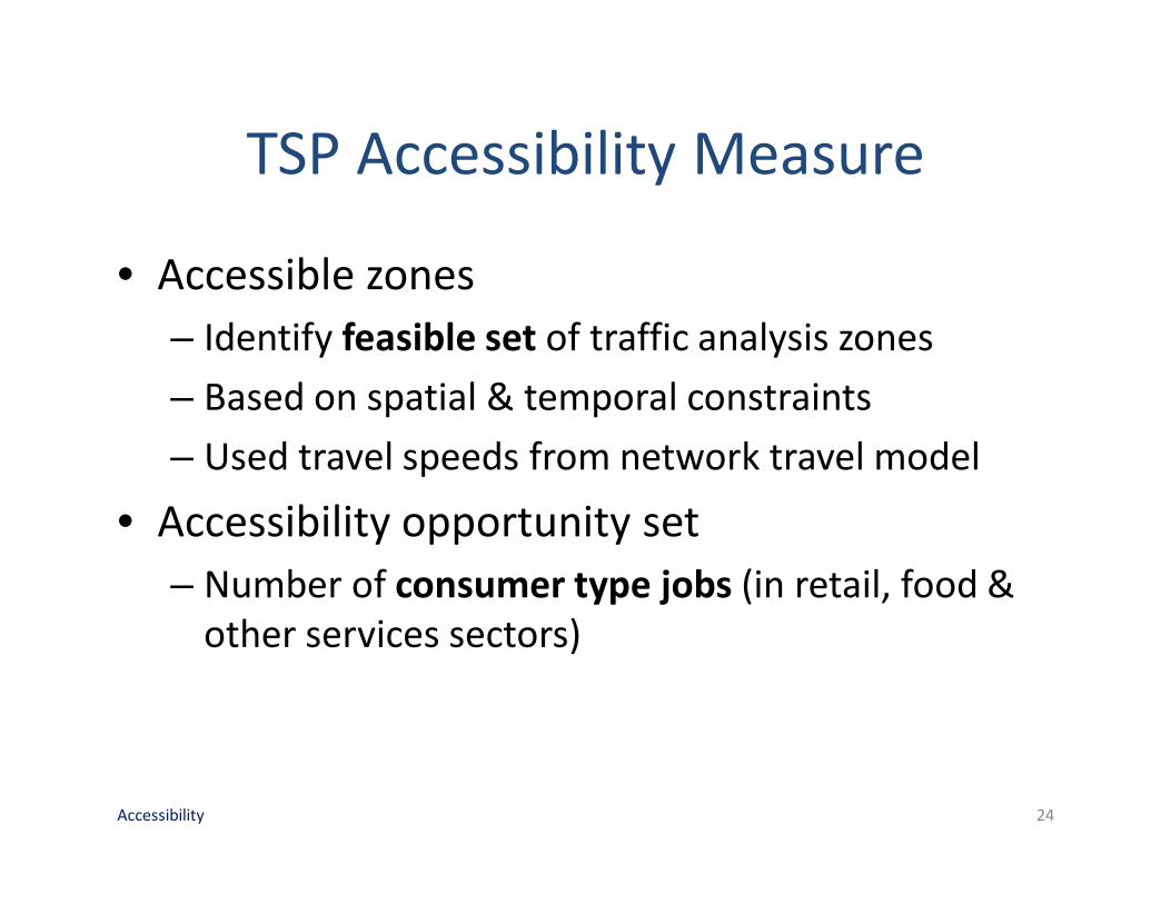
TSP Accessibility Measure

• Accessible zones

– Identify feasible set of traffic analysis zones

– Based on spatial & temporal constraints

– Used travel speeds from network travel model

• Accessibility opportunity set

– Number of consumer type jobs (in retail, food &

other services sectors)

Accessibility 24

Integrated Modeling

Context

Discrete Choice

Analysis


Application

Accessibility

�Model Results

Research Extensions

Questions & Answers

25

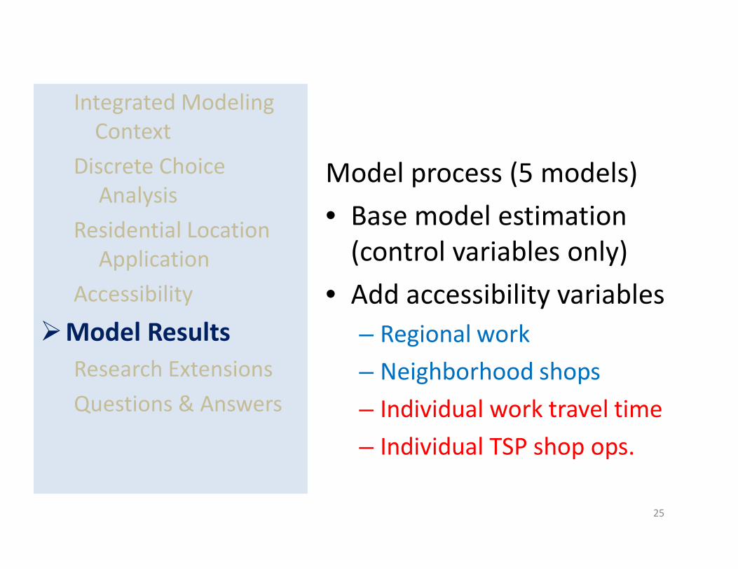
Model process (5 models)

• Base model estimation

(control variables only)

• Add accessibility variables

– Regional work

– Neighborhood shops

– Individual work travel time

– Individual TSP shop ops.

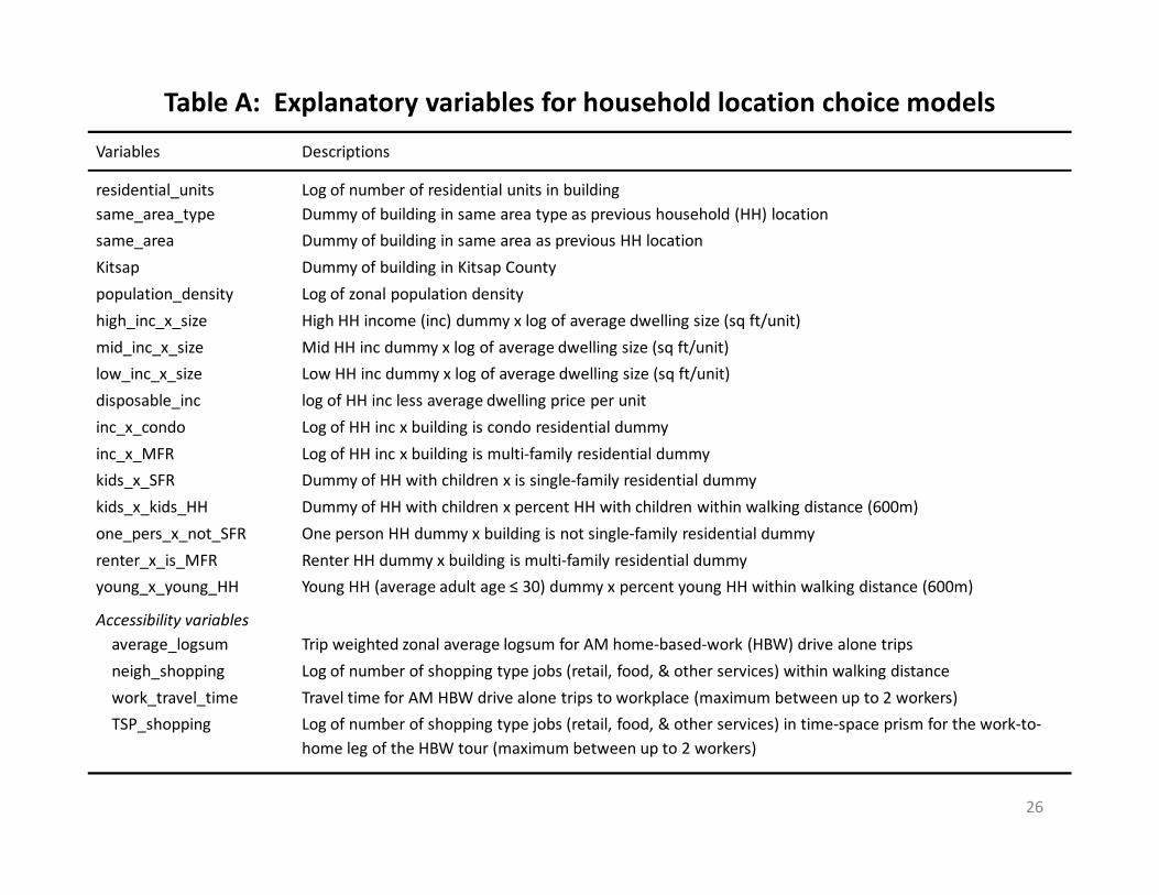
Table A: Explanatory variables for household location choice models

26

Variables Descriptions

residential_units Log of number of residential units in building

same_area_type Dummy of building in same area type as previous household (HH) location

same_area Dummy of building in same area as previous HH location

Kitsap Dummy of building in Kitsap County

population_density Log of zonal population density

high_inc_x_size High HH income (inc) dummy x log of average dwelling size (sq ft/unit)

mid_inc_x_size Mid HH inc dummy x log of average dwelling size (sq ft/unit)

low_inc_x_size Low HH inc dummy x log of average dwelling size (sq ft/unit)

disposable_inc log of HH inc less average dwelling price per unit

inc_x_condo Log of HH inc x building is condo residential dummy

inc_x_MFR Log of HH inc x building is multi-family residential dummy

kids_x_SFR Dummy of HH with children x is single-family residential dummy

kids_x_kids_HH Dummy of HH with children x percent HH with children within walking distance (600m)

one_pers_x_not_SFR One person HH dummy x building is not single-family residential dummy

renter_x_is_MFR Renter HH dummy x building is multi-family residential dummy

young_x_young_HH Young HH (average adult age ≤ 30) dummy x percent young HH within walking distance (600m)

Accessibility variables

average_logsum Trip weighted zonal average logsum for AM home-based-work (HBW) drive alone trips

neigh_shopping Log of number of shopping type jobs (retail, food, & other services) within walking distance

work_travel_time Travel time for AM HBW drive alone trips to workplace (maximum between up to 2 workers)

TSP_shopping Log of number of shopping type jobs (retail, food, & other services) in time-space prism for the work-to-

home leg of the HBW tour (maximum between up to 2 workers)

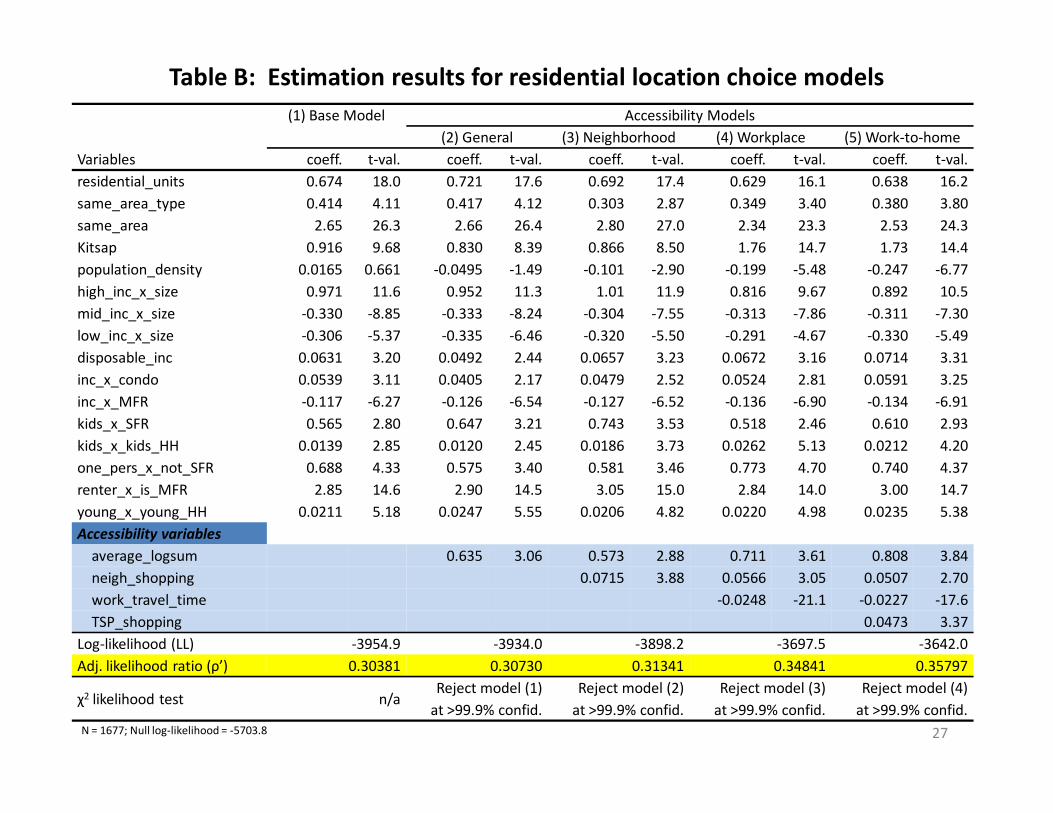
(1) Base Model Accessibility Models

(2) General (3) Neighborhood (4) Workplace (5) Work-to-home

Variables coeff. t-val. coeff. t-val. coeff. t-val. coeff. t-val. coeff. t-val.

residential_units 0.674 18.0 0.721 17.6 0.692 17.4 0.629 16.1 0.638 16.2

same_area_type 0.414 4.11 0.417 4.12 0.303 2.87 0.349 3.40 0.380 3.80

same_area 2.65 26.3 2.66 26.4 2.80 27.0 2.34 23.3 2.53 24.3

Kitsap 0.916 9.68 0.830 8.39 0.866 8.50 1.76 14.7 1.73 14.4

population_density 0.0165 0.661 -0.0495 -1.49 -0.101 -2.90 -0.199 -5.48 -0.247 -6.77

high_inc_x_size 0.971 11.6 0.952 11.3 1.01 11.9 0.816 9.67 0.892 10.5

mid_inc_x_size -0.330 -8.85 -0.333 -8.24 -0.304 -7.55 -0.313 -7.86 -0.311 -7.30

low_inc_x_size -0.306 -5.37 -0.335 -6.46 -0.320 -5.50 -0.291 -4.67 -0.330 -5.49

disposable_inc 0.0631 3.20 0.0492 2.44 0.0657 3.23 0.0672 3.16 0.0714 3.31

inc_x_condo 0.0539 3.11 0.0405 2.17 0.0479 2.52 0.0524 2.81 0.0591 3.25

inc_x_MFR -0.117 -6.27 -0.126 -6.54 -0.127 -6.52 -0.136 -6.90 -0.134 -6.91

kids_x_SFR 0.565 2.80 0.647 3.21 0.743 3.53 0.518 2.46 0.610 2.93

kids_x_kids_HH 0.0139 2.85 0.0120 2.45 0.0186 3.73 0.0262 5.13 0.0212 4.20

one_pers_x_not_SFR 0.688 4.33 0.575 3.40 0.581 3.46 0.773 4.70 0.740 4.37

renter_x_is_MFR 2.85 14.6 2.90 14.5 3.05 15.0 2.84 14.0 3.00 14.7

young_x_young_HH 0.0211 5.18 0.0247 5.55 0.0206 4.82 0.0220 4.98 0.0235 5.38


average_logsum 0.635 3.06 0.573 2.88 0.711 3.61 0.808 3.84

neigh_shopping 0.0715 3.88 0.0566 3.05 0.0507 2.70

work_travel_time -0.0248 -21.1 -0.0227 -17.6

TSP_shopping 0.0473 3.37

Log-likelihood (LL) -3954.9 -3934.0 -3898.2 -3697.5 -3642.0

Adj. likelihood ratio (ρ’) 0.30381 0.30730 0.31341 0.34841 0.35797

χ2 likelihood test n/aReject model (1)

at >99.9% confid.

Reject model (2)

at >99.9% confid.

Reject model (3)

at >99.9% confid.

Reject model (4)

at >99.9% confid.

Table B: Estimation results for residential location choice models

N = 1677; Null log-likelihood = -5703.8 27

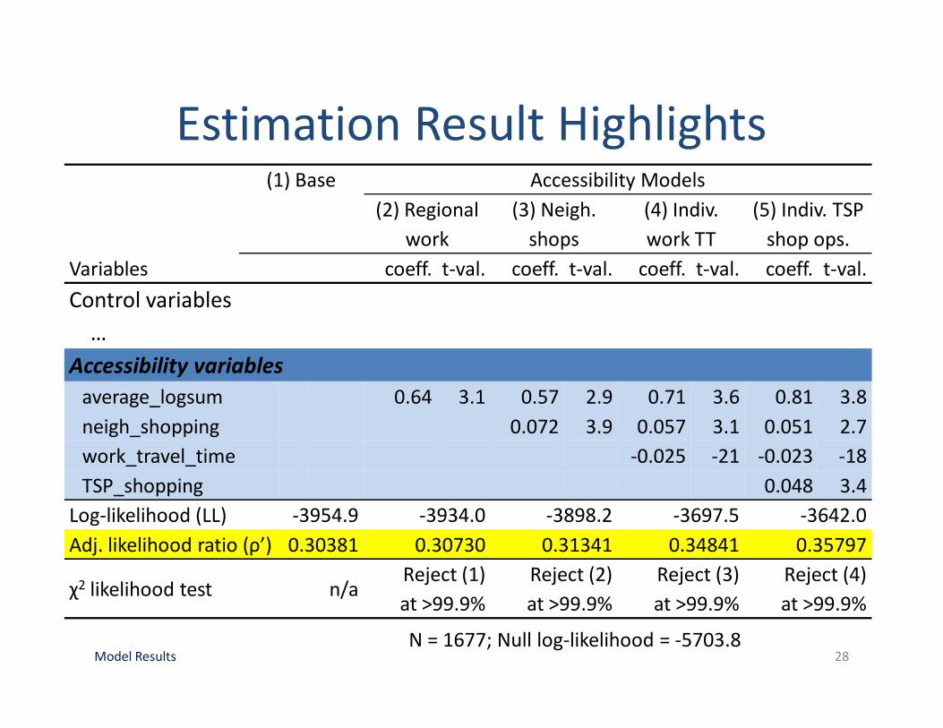
Estimation Result Highlights

Model Results 28

(1) Base Accessibility Models

(2) Regional

work

(3) Neigh.

shops

(4) Indiv.

work TT

(5) Indiv. TSP

shop ops.

Variables coeff. t-val. coeff. t-val. coeff. t-val. coeff. t-val.

Control variables

…


average_logsum 0.64 3.1 0.57 2.9 0.71 3.6 0.81 3.8

neigh_shopping 0.072 3.9 0.057 3.1 0.051 2.7

work_travel_time -0.025 -21 -0.023 -18

TSP_shopping 0.048 3.4

Log-likelihood (LL) -3954.9 -3934.0 -3898.2 -3697.5 -3642.0

Adj. likelihood ratio (ρ’) 0.30381 0.30730 0.31341 0.34841 0.35797

χ2 likelihood test n/aReject (1)

at >99.9%

Reject (2)

at >99.9%

Reject (3)

at >99.9%

Reject (4)

at >99.9%

N = 1677; Null log-likelihood = -5703.8

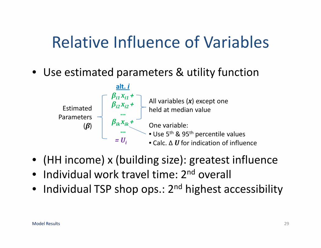
Relative Influence of Variables

• Use estimated parameters & utility function

• (HH income) x (building size): greatest influence

• Individual work travel time: 2nd overall

• Individual TSP shop ops.: 2nd highest accessibility

Model Results 29

alt. i

βi1 xi1 +

βi2 xi2 +

…

βik xik +

…

= Ui

Estimated

Parameters

(β)

All variables (x) except one

held at median value

One variable:

• Use 5th & 95th percentile values

• Calc. Δ U for indication of influence

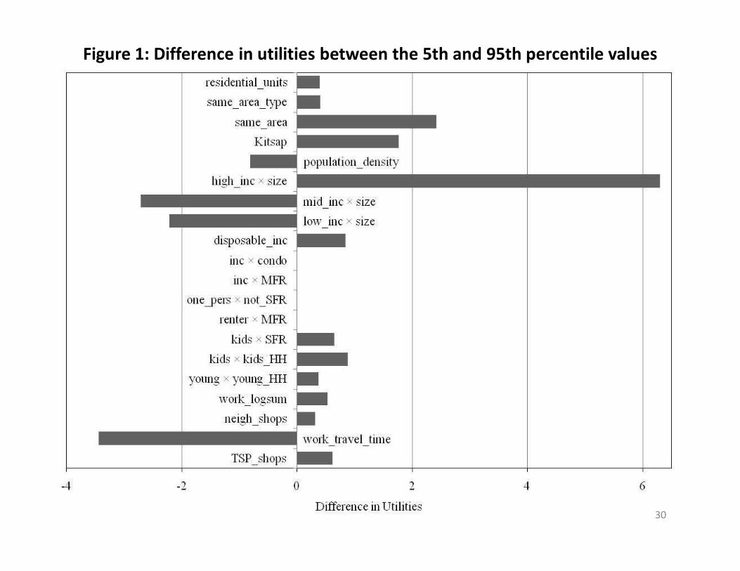
Figure 1: Difference in utilities between the 5th and 95th percentile values

30

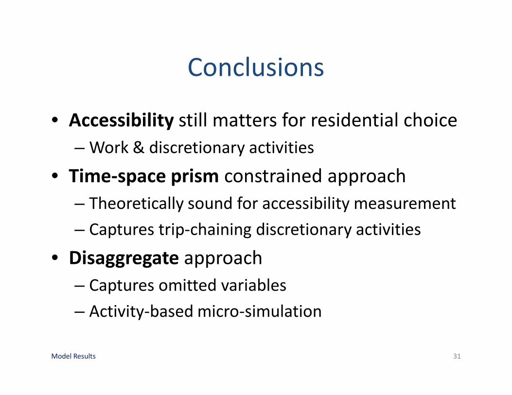
Conclusions

• Accessibility still matters for residential choice

– Work & discretionary activities

• Time-space prism constrained approach

– Theoretically sound for accessibility measurement

– Captures trip-chaining discretionary activities

• Disaggregate approach

– Captures omitted variables

– Activity-based micro-simulation

Model Results 31

Integrated Modeling

Context

Discrete Choice

Analysis


Application

Accessibility

Model Results

�Research Extensions

Questions & Answers

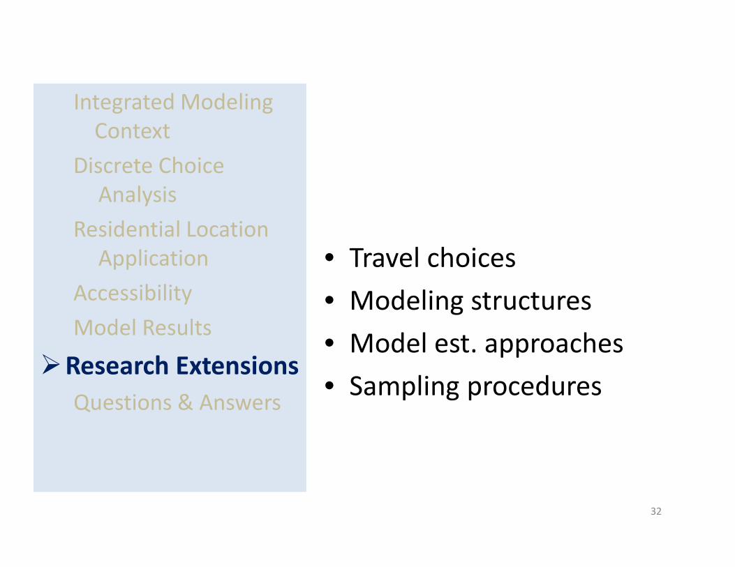
32

• Travel choices

• Modeling structures

• Model est. approaches

• Sampling procedures

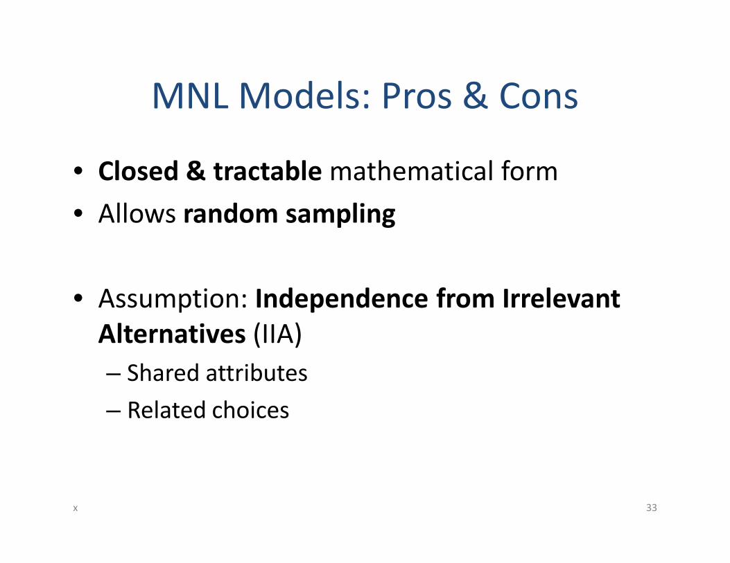
MNL Models: Pros & Cons

• Closed & tractable mathematical form

• Allows random sampling

• Assumption: Independence from Irrelevant

Alternatives (IIA)

– Shared attributes

– Related choices

x 33

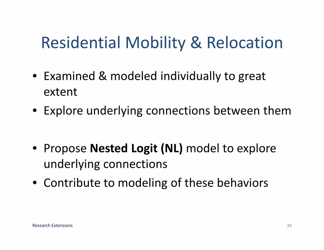
Residential Mobility & Relocation

• Examined & modeled individually to great

extent

• Explore underlying connections between them

• Propose Nested Logit (NL) model to explore

underlying connections

• Contribute to modeling of these behaviors

Research Extensions 34

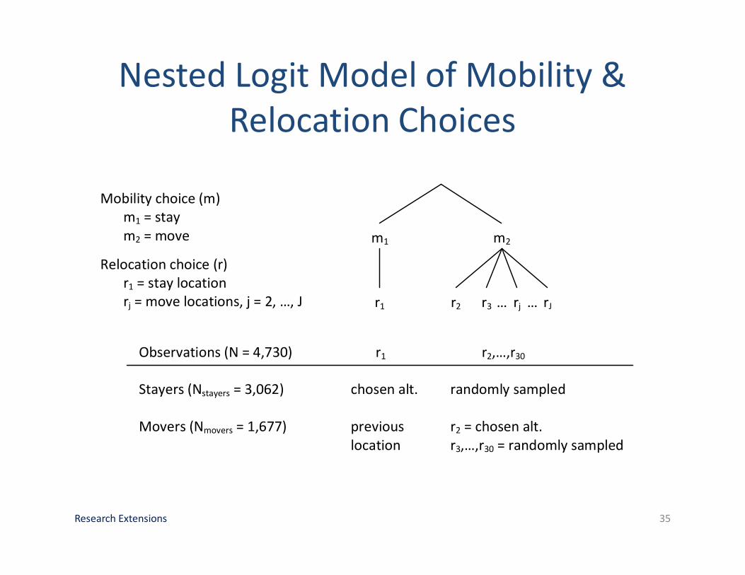
Nested Logit Model of Mobility &

Relocation Choices

Research Extensions 35

m1 m2

r1 r2 r3 rj rJ … …

Mobility choice (m)

m1 = stay

m2 = move

Relocation choice (r)

r1 = stay location

rj = move locations, j = 2, …, J

Observations (N = 4,730) r1 r2,…,r30

Stayers (Nstayers = 3,062) chosen alt. randomly sampled

Movers (Nmovers = 1,677) previous r2 = chosen alt.

location r3,…,r30 = randomly sampled

Acknowledgements

Dr. Paul A. Waddell

Liming Wang

Dept. of Urban Design& Planning

University of Washington

Dr. Ram M. Pendyala

Dept. of Civil & Environmental Engineering

Arizona State University

36

Integrated Modeling

Context

Discrete Choice

Analysis


Application

Accessibility

Model Results

Research Extensions

�Questions &

Answers

37

THANK YOU!

Contact information:

Brian H. Y. Lee

[email protected]

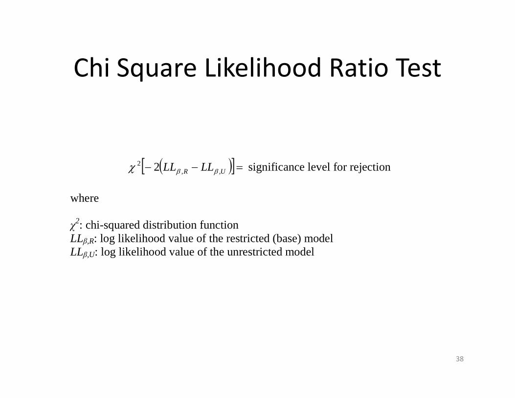
Chi Square Likelihood Ratio Test

38

( )[ ]=−− UR LLLL ,,

2 2 ββχ significance level for rejection

where χ2: chi-squared distribution function LLβ,R: log likelihood value of the restricted (base) model LLβ,U: log likelihood value of the unrestricted model

Re-examining the influence of work and non-work accessibility on residential location choices with a...

Documents

Transcript of Re-examining the influence of work and non-work accessibility on residential location choices with a...