RC 21755 (98001) 30 Ma y2000 Researc h Rep ort -...

RC 21755 (98001) 30 May 2000

Computer Science/Mathematics

IBM Research Report

CSVD: Clustering and Singular Value Decomposi-

tion for Approximate Similarity Searches in High

Dimensional Spaces

Vittorio CastelliIBM Research Division

T.J. Watson Research Center

Yorktown Heights, New York

e-mail: [email protected]

Alexander ThomasianCS&E Dept. at Univ. of Connecticut,

One University Place

Stamford CT 06901

e-mail: [email protected].

Chung-Sheng LiIBM Research Division

T.J. Watson Research Center

Yorktown Heights, New York

e-mail: [email protected]

LIMITED DISTRIBUTION NOTICE

This report has been submitted for publication outside of IBM and will probably be copyrighted is accepted for publi-

cation. It has been issued as a Research Report for early dissemination of its contents. In view of the transfer of copyrightto the outside publisher, its distribution outside of IBM prior to publication should be limited to peer communications and

speci�c requests. After outside publication, requests should be �lled only by reprints or legally obtained copies of the arti-cle (e.g., payment of royalties). Some reports are available at http://domino.watson.ibm.com/library/CyberDig.nsf/home.

Copies may requested from IBM T.J. Watson Research Center, 16-220, P.O. Box 218, Yorktown Heights, NY 10598 orsend email to [email protected].

IBMResearch Division

Almaden � Austin � Beijing � Haifa � T.J. Watson � Tokyo � Zurich

CSVD: Clustering and Singular Value Decomposition

for Approximate Similarity Searches in High

Dimensional Spaces

Vittorio Castelli, Alexander Thomasian and Chung-Sheng Li

June 12, 2000

Abstract

High-dimensionality indexing of feature spaces is critical for many data-intensive

applications such as content-based retrieval of images or video from multimedia

databases and similarity retrieval of patterns in data mining. Unfortunately, even

with the aid of the commonly-used indexing schemes, the performance of near-

est neighbor (NN) queries (required for similarity search) deteriorates rapidly with

the number of dimensions. We propose a method called Clustering with Singular

Value Decomposition (CSVD) to reduce the number of index dimensions, while

maintaining a reasonably high precision for a given value of recall. In CSVD, ho-

mogeneous points are grouped into clusters such that the points in each cluster

are more amenable to dimensionality reduction than the original dataset. Within-

cluster searches can then be performed with traditional indexing methods, and we

describe a method for selecting the clusters to search in response to a query. Ex-

periments with texture vectors extracted from satellite images show that CSVD

achieves signi�cantly higher dimensionality reduction than plain SVD for the same

Normalized Mean Squared Error (NMSE). Conversely, for the same compression

ratio, CSVD results in a decrease in NMSE with respect to simple SVD (a 6-

fold decrease a 10:1 compression ratio). This translates to a higher e�ciency in

processing approximate NN queries, as quanti�ed through experimental results.

1 Introduction

Similarity-based retrieval has become an important tool for searching image and video

databases, especially when the search is based on content of images and videos, and

is performed using low-level features, such as texture, color histogram and shape. Theapplication areas of this technology are quite diverse, as there has been a proliferation of

databases containing photographic images [34, 24, 30], medical images, [16], video clips

[32], geographically referenced data [31], and satellite images [29, 22].

E�cient similarity search invariably requires precomputed features. The length of the

feature vectors can be potentially large. For example, the local color histogram of anRGB image (obtained by quantizing the colors from a sliding window) has usually atleast 64 dimensions, and often the dimensionality of texture vectors is 50 or more [21].Similarity search based on features is equivalent to a nearest neighbor (NN) query in the

high-dimensionality space of the feature vectors. NN search based on sequential scan oflarge �les, or tables, of feature vectors is computationally too expensive and has a longresponse time.

Multidimensional indexing structures, which have been investigated intensively in re-

cent years [14], seem to be the obvious solution to this problem. Unfortunately, as a result

of a combination of phenomena, customarily known as the \curse of dimensionality" [9,Chapter 1], the e�ciency of indexing structures deteriorates rapidly as the number ofdimensions increases [5, 4, 14]. A potential solution is therefore to reduce the number ofdimensions of the search space before indexing the data. The challenge is to achieve index

space compression (which in general results in loss of information) without a�ecting infor-mation retrieval performance. In this paper, we use the terms \index space compression"and \data compression" to denote the reduction of the average number of dimensions

used to describe each entry in the database.

Dimensionality reduction methods are usually based on a linear transformations fol-lowed by the selection of a subset of features, although nonlinear transformations are also

possible. Techniques based on linear transformations, such as the Karhunen-Loeve (KL)transform, the Singular Value Decomposition (SVD) method, and Principal Component

Analysis (PCA) [17, 12], have been widely used for dimensionality reduction and datacompression [19] and form the basis of our study. Nonlinear multidimensional scaling for

dimensionality reduction [2], and other fast methods, such as FastMap [13, 12], have alsobeen investigated.

SVD is shown to be very e�ective in compressing large tables with numeric values in

2

[19], where a 40:1 compression ratio is achieved, with an average error of less than 5%.

This method outperforms a clustering-based method, and a spectral method [12]. SVD

−4

−2

0

2

4

−4

−2

0

2

4−4

−3

−2

−1

0

1

2

3

4

(a) −4−3−2−101234−4−2024

−4

−3

−2

−1

0

1

2

3

4

(b)

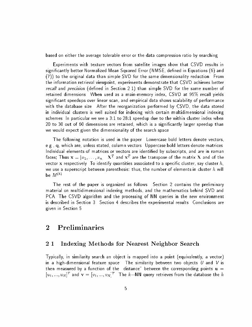
Figure 1: Intuition about using clustering to assist dimensionality reduction. The synthetic

data was obtained by independent sampling from a mixture of three 3-dimensional Gaussian

distributions.

relies on \global" information derived from all the vectors in the dataset. Its application isthereforemore e�ective when the datasets consist of \homogeneously distributed vectors",or, better, of datasets the distribution of which is well captured by the centroid and thecovariance matrix. This is the case discussed in Korn [19], where the authors deal with

outliers by storing them separately and searching them exhaustively.

For databases with \heterogeneously" distributed vectors, more e�cient representation

can be generated by subdividing the vectors into groups, each of which is then charac-terized by a di�erent set of statistical parameters. In particular, this is the case if the

data comes from a set of populations each of which is homogeneous in the sense de�ned

above. As a more tangible example, consider Fig. 1: here, a set of points in 3-dimensionalspace is clustered into three relatively at and elongated ellipsoids. The \ellipsoids" are

obtained by independent sampling from synthetically generated 3-dimensional Gaussiandistributions. Figure 1(b) shows clearly that for two of the ellipsoids, most of the variance

is captured by two of the three dimensions. Then, the points in each ellipsoid can berepresented rather accurately in two dimensions. Note, though, that reducing the dimen-

sionality of the entire dataset, without partitioning the data �rst, would result in large

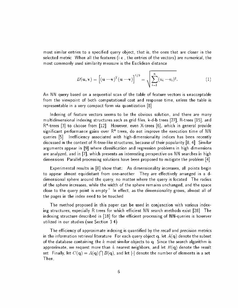
approximation errors. Real data can display the same behavior: consider for example the

scatterplot, displayed in Figure 2(a), of three texture features extracted from a satellite

3

image of the Earth, or the scatterplot of Figure 2(b) showing measures acquired from a

computer for capacity management purposes.

In statistics, often data is described by decomposing it into a mixture of Gaussiandistributions, and methods exist to solve the estimation problem [10]. Young and Liu [35]

relied on this insight to propose a method for lossless data compression, called multilin-

ear compression, consisting of clustering followed by singular value decomposition. The

assumption underlying multilinear compression is that some of the cluster actually lie on

lower-dimensional subspaces. More recently, Aggarwal and Yu [1] proposed a fast methodfor combining clustering and dimensionality reduction.

1.82

2.22.4

2.62.8

0

0.1

0.2

0.3

0.40

1000

2000

3000

4000

5000

6000

7000

FRACTAL DIMENSIONMeanASMSGLD

Mea

nCO

NS

GLD

−2 0 2 4 6 8 10 12x 10

8

−1

0

1

2

3

4

5

x 108

−1

0

1

2

3

4

5

6

x 106

(a) (b)

Figure 2: Scatterplot of a three-dimensional feature vector set computed from a satellite

image, showing clustering behavior (a). Projections on 3-dimensional space of 4025 100-

dimensional vectors of measurements acquired from a computer, for capacity management

purposes. The �gure shows that the distribution of the measured quantities is really a

mixture of di�erent distributions, each of which is characteristic of a particular load or class

of loads (b).

This paper introduces a newmethod, Clustering Singular Value Decomposition (CSVD),

for indexing data by reducing the dimensionality of the space. This method consists ofthree steps: partitioning the data set using a clustering technique [11] (see Section 4),

computing independently the SVD of vectors in each cluster to produce a vector space of

transformed features with reduced dimensionality, and constructing an index for the trans-

formed spaced. An iterative procedure then discovers the \optimal" degree of clustering

4

based on either the average tolerable error or the data compression ratio by searching.

Experiments with texture vectors from satellite images show that CSVD results in

signi�cantly better Normalized Mean Squared Error (NMSE, de�ned in Equations (6) and(7)) to the original data than simple SVD for the same dimensionality reduction. From

the information retrieval viewpoint, experiments demonstrate that CSVD achieves better

recall and precision (de�ned in Section 2.1) than simple SVD for the same number ofretained dimensions. When used as a main-memory index, CSVD at 95% recall yields

signi�cant speedups over linear scan, and empirical data shows scalability of performance

with the database size. After the reorganization performed by CSVD, the data storedin individual clusters is well suited for indexing with certain multidimensional indexing

schemes. In particular we see a 3:1 to 28:1 speedup due to the within-cluster index when20 to 30 out of 60 dimensions are retained, which is a signi�cantly larger speedup thanwe would expect given the dimensionality of the search space.

The following notation is used in the paper. Lowercase bold letters denote vectors,

e.g., q, which are, unless stated, column vectors. Uppercase bold letters denote matrices.Individual elements of matrices or vectors are identi�ed by subscripts, and are in romanfaces; Thus x = [x1; : : : ; xn]. X

T and xT are the transpose of the matrix X and of the

vector x respectively. To identify quantities associated to a speci�c cluster, say cluster h,we use a superscript between parenthesis: thus, the number of elements in cluster h willbe M (h).

The rest of the paper is organized as follows. Section 2 contains the preliminary

material on multidimensional indexing methods, and the mathematics behind SVD andPCA. The CSVD algorithm and the processing of NN queries in the new environmentis described in Section 3. Section 4 describes the experimental results. Conclusions aregiven in Section 5.

2 Preliminaries

2.1 Indexing Methods for Nearest Neighbor Search

Typically, in similarity search an object is mapped into a point (equivalently, a vector)

in a high-dimensional feature space. The similarity between two objects U and V is

then measured by a function of the \distance" between the corresponding points u =

[u1; :::; uN]T and v = [v1; :::; vN]

T . The k�NN query retrieves from the database the k

5

most similar entries to a speci�ed query object, that is, the ones that are closer in the

selected metric. When all the features (i.e., the entries of the vectors) are numerical, the

most commonly used similarity measure is the Euclidean distance

D(u;v) =h(u� v)

T(u� v)

i1=2=

vuutnXi=1

(ui � vi)2: (1)

An NN query based on a sequential scan of the table of feature vectors is unacceptablefrom the viewpoint of both computational cost and response time, unless the table is

representable in a very compact form via quantization [8].

Indexing of feature vectors seems to be the obvious solution, and there are manymultidimensional indexing structures such as grid �les, k-d-b trees [27], R-trees [15], andR*-trees [3] to choose from [12]. However, even X-trees [6], which in general providesigni�cant performance gains over R*-trees, do not improve the execution time of NNqueries [5]. Ine�ciency associated with high-dimensionality indices has been recently

discussed in the context of R-tree-like structures, because of their popularity [8, 4]. Similararguments appear in [9] where classi�cation and regression problems in high dimensionsare analyzed, and in [7], which presents an interesting perspective on NN searches in high

dimensions. Parallel processing solutions have been proposed to mitigate the problem [4].

Experimental results in [8] show that: \As dimensionality increases, all points beginto appear almost equidistant from one-another. They are e�ectively arranged in a d-dimensional sphere around the query, no matter where the query is located. The radiusof the sphere increases, while the width of the sphere remains unchanged, and the space

close to the query point is empty." In e�ect, as the dimensionality grows, almost all of

the pages in the index need to be touched.

The method proposed in this paper can be used in conjunction with various index-ing structures, especially R-trees for which e�cient NN search methods exist [28]. The

indexing structure described in [18] for the e�cient processing of NN-queries is however

utilized in our studies (see Section 3.4).

The e�ciency of approximate indexing is quanti�ed by the recall and precision metrics

in the information retrieval literature. For each query object q, let A(q) denote the subset

of the database containing the k most similar objects to q. Since the search algorithm is

approximate, we request more than k nearest neighbors, and let B(q) denote the result

set. Finally, let C(q) = A(q)TB(q), and let j�j denote the number of elements in a set.

Then,

6

� Recall (R) is the fraction of retrieved objects that are among the k closest objects

to q, namely

R =jC(q)j

jA(q)j: (2)

� Precision (P ) is the fraction of the k closest points to q that are retrieved by the

algorithm, i.e.,

P =jC(q)j

jB(q)j: (3)

When the retrieval algorithm is approximate, one can increase the recall by increasing thesize of B(q), but this in general reduces the precision, and vice versa.

2.2 Singular Value Decomposition

In this subsection, the well-known singular value decomposition (SVD) method is reviewedin order to establish the necessary notations for the rest of the paper. Consider an M�N

matrix X the columns of which are correlated. Let � be the column mean of X = [xi;j],

(�j = (1=M)P

M

i=1 xi;j; for 1 � j � N ,) and let 1M be a column vector of length M

with all elements equal to 1. SVD expresses X � 1M�T as a product of an M � N

column orthonormal matrix U (i.e., UTU = I, where I is the identity matrix), an N �N

diagonal matrix S containing the singular values, and an N � N real unitary matrix V[26]:

X� 1M�T = USV

T (4)

The columns of the matrixV are the eigenvalues of the covariance matrixC of X, de�nedas

C =1

MX

TX� ��

T = V�VT: (5)

The matrix C is positive-semide�nite, hence it has N nonnegative eigenvalues and N

orthonormal eigenvectors. Without loss of generality, let the eigenvalues of C be ordered

in decreasing order, i.e., �1 � �2 � ::: � �N : The trace (�) of C remains invariant under

rotation, i.e., �4=P

N

j=1 �2j=P

N

j=1 �j: The fraction of variance associated with the jth

eigenvalue is �j=�: The singular values are related to the eigenvalues by: �j = s2j=M

or sj =pM�j : The eigenvectors constitute the principal components of X; hence the

transformationY = V(X�1M�T ) yields zero-mean, uncorrelated features. PCA retains

the features corresponding to the p highest eigenvalues. Consequently for a given p it

7

minimizes the Normalized Mean Squared Error which is denoted by NMSE, and is de�ned

as

NMSE =

PM

i=1

PN

j=p+1 y2i;jP

M

i=1

PN

j=1 y2i;j

=

PM

i=1

PN

j=p+1 y2i;jP

M

i=1

PN

j=1 (xi;j � �j)2(6)

where the column mean � is computed in the original reference frame.

This property makes SVD the optimum linear transformation for dimensionality re-

duction, when the p dimensions corresponding to the highest eigenvalues are retained.

Several heuristics to select p are given in [17], e.g., retain transformed features whose

eigenvalues are larger than the average �=M: This may be unsatisfactory, for instancewhen an eigenvalue slightly less than �=M is omitted. In this paper, p is selected sothat NMSE does not exceed a threshold that yields acceptable e�ciency in approximatesearching.

The p columns of the Y = XV matrix corresponding to the highest eigenvalues areretained, the remaining discarded. This is tantamount to �rst projecting the vectors in Yonto the k-dimensional hyperplane passing through � and spanned by the eigenvectors ofC corresponding to the largest eigenvalues, and then representing the projected vector in

the reference system having as origin � and as coordinate axes the eigenvectors of C.

In the Appendix we compare the approach in this paper with that of a recent paper [19],showing that, for the same storage space and approximation error, ours is computationallymore e�cient.

3 The CSVD Algorithm

3.1 Preprocessing of Dataset

Before constructing the index, care should be taken to appropriately scale the numericalvalues of the di�erent features used in the index. In the case of texture features (used asthe test dataset for this paper) some quantities have a small range (the texture feature

known as fractal dimension varies between 2 and 3), while others can vary signi�cantly

more (the dynamic range of the variance of the gray-level histogram can easily exceed105).

In this paper, we assume that all the features contribute equally to determine the

similarity between di�erent vectors. Consequently, the N columns of the table X are

8

separately studentized (by subtracting from each column j its empirical mean �j and

dividing the result by an estimator of its standard deviation �̂j) to obtain columns with

zero mean and unit variance: x0

i;j= (xi;j � �j)=�̂j ; 1 � j � N and 1 � i � M;

where the number of rows M is the number of records in the database table. Note that

the studentization is done only once, on the original table X, and it is not repeated afterthe clustering and dimensionality reduction steps described in the following section.

After studentization, the sum of the squared entries of the table is computed as

E =P

M

i=1

PN

j=1

�x

0

i;j

�2, which is used as denominator of equation (6) to compute the

NMSE. Thus, without loss of generality, we will assume that the columns of the table X

have zero mean and unit variance.

3.2 Index Construction

Before describing the index construction algorithm, we provide the de�nition of the NMSE

resulting from substituting the table X = [xi;j]M�N , whose columns have zero mean, with

a di�erent table X0

= [x0

i;j]M�N , without changing the reference frame:

NMSE =

PM

i=1

PN

j=1(xi;j � x0

i;j)2

PM

i=1

PN

j=1x2i;j

: (7)

This de�nition is valid for any mapping from X to X0

, including the one used by CSVD.The basic steps of the CSVD index construction are partitioning of the database, rotationof the individual clusters onto an uncorrelated orthogonal coordinate system, dimension-

ality reduction of the rotated clusters, and within-cluster index construction.

1. The partitioning step takes as its input the table X and divides the rows into H

homogeneous groups, or clusters, X(h); 1;� h � H, having sizes M (1)

; : : : ;M(H).

The number of clusters can be a parameter or can be determined dynamically. In thecurrent implementation, classical clustering methods such as LBG [23] or K-means

[11] are used. These are vector-quantization-style algorithms [23], that generateclusters containing vectors which are similar to each other in the Euclidean metric

sense. It is known that these methods, albeit optimal, do not scale well with thesize of the database. If the speed of the index construction is an important factor,

one can use suboptimal schemes, such as tree-structured vector quantizers (TSVQ)

[25], or sub-sampling schemes to limit the number of data point used to train the

quantizer, i.e., to construct a partition of the database.

9

2. The rotation step is carried out independently for each of the clustersX(h); 1 � h �

H. The corresponding centroid �(h) is subtracted from each group of vectors X(h),

and the eigenvector matrix V(h) and the eigenvalues �(h)1 ; : : : ;� �

(h)

N, (ordered by

decreasing magnitude), are computed as described in Section 2.2. The vectors of

X(h) are then rotated in the uncorrelated reference frame having the eigenvectors

as coordinate axes, to produce ~X(h).

3. The dimensionality reduction step is performed using a procedure that considers allthe clusters. To understand the e�ects of discarding a set of dimensions within a

speci�c cluster (say the hth, containing M (h) vectors), recall that this is equivalent

to replacing the vectors with their projections onto the subspace passing through thecentroid of the cluster and de�ned by the retained eigenvectors. This approximation

a�ects the numerator of Equation (7), which is increased by the sum of the squaredistances between the original points and their projections. Since the dimensions areuncorrelated, calling �

(h)

(1); : : : ; �

(h)

(p)the retained eigenvalues, one can easily see that

the ith dimension adds �(h)

(i)M(h) to the numerator. We use the notation Y

(h) to

denote the representation of X(h) in the translated, rotated and projected reference

frame.

We have implemented four avors of dimensionality reduction.

(a) Dimensionality reduction to a �xed number of dimensions: the number p of

dimensions to retain is provided as input; the p dimensions of each clustercorresponding to the largest eigenvalues are retained.

(b) Independent reduction with target NMSE (TNMSE): clusters are analyzedindependently. From each cluster h the minimum number p(h) of dimensionsare retained for which

Pp

i=1 �(h)i

� TNMSEP

N

i=1 �(h)i. Thus, the average

approximation is roughly the same for all clusters.

(c) Global reduction to an average number of dimensions: the average number

of dimensions to retain, p, is provided as input. All the clusters are analyzed

together. The products of the eigenvalues �(h)i

times the size of the corre-

sponding clustersM (h) are computed and sorted in ascending order, producingan ordered list of H � N values. Discarding a value M (h)

�(h)i

corresponds to

removing the ith of the dimensions of the hth cluster, increases the numera-

tor of the NMSE by M (h)�(h)i, and decreases the average number of retained

dimensions by M (h)=M . The �rst value in the ordered list is the dimension

that has the smallest e�ect on the NMSE, while the last value has the largeste�ect. The �rst ` values are discarded, where ` is the largest number for which

10

the average number of retained dimensions is larger than or equal to p. This

is the default approach when the number of dimensions is provided as input.

(d) Global reduction to a target NMSE: As in the previous case, all the products

M(h)�(h)i

of the individual eigenvalues times the number of vectors in thecorresponding clusters are computed, and sorted in ascending order. The �rst

`0

values are discarded, where `0

is the largest number for which the NMSE is

less than or equal to TNMSE. This is the default approach when TNMSE isprovided as input.

4. The within-cluster index construction step operates separately on each cluster Y(h).

In the current implementation, we do not specify a new methodology for this step,rather we rely on any of the known indexing technique. Due to the dimensionality

reduction, each cluster is much more amenable to e�cient indexing than the entiretable. In this paper, the very e�cient k-NN method proposed by Kim and Park[18] is used for this purpose, due to its good performance even in medium-high

dimensionality spaces (more details are available in [33]).

Sometimes the algorithm can bene�t from an initial rotation of the entire dataset into un-correlated axes (with or without dimensionality reduction), for instance, when the columnsof the data table are indeed homogeneously strongly correlated. In this case, an initial

application of step 3 should precede the clustering. In other cases dimensionality reductioncan conceal cluster structures [11], or the clustering algorithm is insensitive to the orienta-

tion of the axes, as in the case of LBG [23] (which is a vector-quantization style clustering

method), and no initial transformation of the data should be performed. The index con-struction algorithm can be applied recursively: Steps 1-3 can be recursively repeated untilterminating conditions are met. The resulting indexing structure can be represented as atree. The data is stored at the leaves, each of which has its own within-cluster index.

The goals of simultaneously minimizing the size of the resulting index and maximizing

the speed of the search are somewhat contradictory. Minimizing the size of the index by

aggressive clustering and dimensionality reduction is very bene�cial when the database is

very large. On the other hand, aggressive clustering and dimensionality reduction can alsoforce the search algorithm to visit more clusters, thus reducing the bene�ts of computing

the distances with fewer dimensions.

Since the search is approximate, di�erent index con�gurations should be compared

in terms of recall (Equation (2) and precision (Equation (3)). These two metrics are

di�cult to incorporate into an optimization procedure, because their values can only bedetermined experimentally (see Section 4). An optimization algorithm is required to select

11

the number of clusters and the number of dimensions to be retained for given constraints

on precision and recall. This problem can be solved in two steps by noting that both recall

and precision are monotonically decreasing functions of the NMSE. Hence an index that

minimizes NMSE can be designed for a given data compression objective. If the value

of NMSE is large, the optimization with a less stringent data compression objective isrepeated. The index is then tested to con�rm whether it yields satisfactory precision and

recall. This is done by constructing a test set, searching for the k nearest neighbors of

its elements using an exact method and the approximate index, thus estimating precision

and recall. If the performance is not adequate, the input parameters for designing the

index are respeci�ed. Including this last step as part of the optimization is possible, butwould have made the initial index design step very lengthy.

A direct consequence of the dimensionality reduction of the index space is the reduction

of its index size. The size of the index is a�ected by the e�ciency of data representationand the size of the clustering and SVD information, namely, the V(h) matrices for coordi-nate transformation and the number of dimensions retained by the SVD. For large tables

and a non-aggressive clustering strategy, the clustering and SVD information are a negli-gible fraction of the overall data. Thus, we de�ne the index volume as the total number

of entries preserved by the index. The original volume is then de�ned as V04= M � N ,

i.e., it is equal to the number M of vectors in the table times the original number N

of dimensions. Given H clusters, denoting with M(h) the number of points and with

p(h) the number of retained dimensions in cluster h, the volume after steps 1 and 3 isV1 =

PH

h=1M(h)p(h). The fraction of volume retained is then simply Fvol = V1=V0 and

the mean number of retained dimensions is N � Fvol. A procedure which determines an

\optimal" number of clusters (H) for a given Fvol so as to minimize NMSE is describedbelow.

� First note that the reduction in the volume objective directly translates to the mean

number of dimensions in the resulting index: p(Fvol) = V1=M:

� Consider increasing values of H, and for each H use a binary search to determine

the value NMSE(H) corresponding to p(Fvol) 2 [V1=M � :5; V1=M � :5].

� A point of diminishing returns is reached asH increases, and the search is terminated

when NMSE(H+�)=NMSE(H) � (1+�) (where the parameters � and � are providedby the user. In our experiments we have used � = :01 and, trivially � = 1):

In e�ect, although NMSEmin is not achieved exactly by the procedure, selecting the smaller

H will result in a smaller index size when the size of the meta-data �le is also taken into

12

account.

The minimum value for NMSE (NMSEmin) for the input parameter Fvol varies with

the dataset. A relatively reasonable Fvol (based on experience with similar datasets) mayresult in an NMSEmin which is too large to sustain e�cient processing of NN queries.

The user can specify a larger value for Fvol to ensure a smaller NMSEmin: Alternatively,

a smaller Fvol may be considered if NMSEmin is too small.

After the index is created additional tests are required to ensure that the index providesa su�cient precision for a given recall. The query points may correspond to randomly

selected vectors from the input table. The index is unsatisfactory if the mean precision(P ) over a test set of samples is smaller than a pre-speci�ed threshold.

3.3 Searching for the Nearest Neighbors

3.3.1 Exact queries

In an exact search all the element of the table that are equal to an N�dimensionalquery point q must be retrieved. In response to an exact search, q is �rst studentized

with the same coe�cients used for the entire database, thus yielding q0

. If an initialrotation and dimensionality reduction was performed before the clustering step 1 duringthe index construction, the vector q

0

is rotated to produce ~q0

= q0

V, and all the discardeddimensions are set to zero (recall that the dataset is studentized, thus � is now the origin

of the Euclidean coordinate system). The preprocessed query vector is henceforth denoted

by q̂.

The cluster to which q̂ belongs, referred to as the primary cluster, is then found. Theactual details of this step depend on the selected clustering algorithm. For LBG, which

produces a conditionally optimal tessellation of the space given the centroid selection, theindex of the primary cluster is } = argmin

h

�D(q̂;�(h))

, (where D (�; �) is the Euclidean

distance,) i.e., q̂ belongs to the cluster with the closest centroid. For our implementation

of LBG, the computational cost is O(N �H), where again H is the number of clusters. Fortree-structured vector quantizers (TSVQ) the labeling step is accomplished by following a

path from the root of a tree to one of its leaves, and if the tree is balanced, the expected

computational cost is O(N � logH). Once the primary cluster is determined, q̂ is rotated

into the associated reference frame. Using the notation developed in the previous section,

we denote by q0(})

= (q̂ � �(}))V(}) the representation of q̂ in the reference frame

associated with cluster }. Then, the projection step onto the subspace is accomplished

13

by retaining only the relevant dimensions, thus yielding q(}). Finally, the within-cluster

index is used to retrieve all the records that are equal to q(}).

By construction, the CSVD index can result in false hits; however, misses are notpossible. False hits can then be �ltered in a post-processing phase, by comparing q with

the original versions of the retrieved records.

3.3.2 Similarity queries

The emphasis in this paper is on similarity searches, and in particular, on retrieving fromthe database the k nearest neighbor of the query point q. The �rst steps of a similaritysearch consist of the preprocessing described in the exact search context, the identi�cation

of the primary cluster, and the projection of the query point onto the associated subspace

to yield q(}). After the query point is projected onto the subspace of the primary cluster,a k-nearest neighbor search is issued using the within-cluster index.

Unlike the exact case, though, the search cannot be limited to just one cluster. Ifthe query point falls near the boundaries of two or more clusters (which is a likely event

in high dimensionality spaces), or if k is large, some of the k nearest neighbors of thequery point can belong to neighboring clusters. It is clearly undesirable to search allthe remaining clusters, since only a few of them are candidates, while the others cannotpossibly contain any of the neighbors of q. A modi�ed branch-and-bound approach is

adopted. In particular, the simple strategy illustrated in Figure 3 is used to determine

the candidates. After searching the primary cluster, k points are retrieved. The distancebetween q and the farthest retrieved record is an upper bound to the distance between q

and its kth neighbor nk. A cluster is not a candidate, and thus can be discarded, if all its

points are farther away from q than nk. To identify non-candidate clusters, the clusterboundaries are approximated by minimum bounding spheres. The distance of the farthest

point in cluster Ci from its centroid is referred to as its radius, is denoted by Ri, and is

computed during the construction of the index.

A cluster is discarded if the distance between its hyper-sphere and q is greater than

D(q;nk), and considered a candidate otherwise (See Figure 3). Note, incidentally, that q

can belong to the hyper-sphere of a cluster (such as, but not necessarily only, the primary

cluster), in which case the distance is by de�nition equal to zero. The distances between

q and the hyper-spheres of the clusters are computed only once. The computational costis O(N �H), and the multiplicative constant is very small. The candidate cluster (if any)with hyper-sphere closer to q is visited �rst. Ties are broken by considering the distances

14

C

C

C

Cr

r

i

l

j

k

R

R

R

R

i

l

j

k

1

0

q

Figure 3: Searching nearest neighbors across multiple clusters. The �gure shows three

clusters, Ci, Cj , Ck and Cl. The query point is denoted by q. If D(q;nk) = r0, cluster

Ci, Cj and Ck are candidates, while Cl is discarded. If, after searching Ci, the updated

D(q;nk) becomes equal to r1, cluster Ck is removed from the candidate set.

15

between q and centroids, as is the case, for instance, if q belongs to the hyper-spheres of

several clusters. In the highly unlikely case that further ties occur (i.e., q is equidistant

from the hyper-spheres and the centroids of two clusters), the cluster with smaller index is

visited �rst. If the current NNs list is updated during the within-cluster search, nk changes

and D(q;nk) is reduced. Thus, the list of non-visited candidates must be updated. Thesearch process terminates when the candidate list is empty.

An alternative, simpler, strategy is outlined below. Denote by di;j the distance between

the centroids of two clusters Ci and Cj, and de�ne the distance between two clusters as

the distance between their hyper-spheres, i.e., di;j � Ri � Rj . While di:j > Ri + Rj istrue in some cases, di;j < Ri + Rj is also possible. It is even possible for the K-means

method to generate one cluster embedded inside another [20]. During the search phase,the clusters that intersect the primary cluster are checked in increasing order of distance,while clusters with positive distances from the target cluster are not checked. This simple

strategy has the advantage of being static (since di;j are compute at index-constructiontime), but does not guarantee that all the relevant clusters are visited.

Finally, more complex approaches can rely on the approximation of the cluster bound-aries by more complex surfaces, such as, for instance, hyper-ellipsoids aligned with the

eigenvalues of the cluster. Using better approximations of the cluster boundaries reducesthe possibility of visiting non-candidate clusters, however it can signi�cantly complicatethe identi�cation of the candidates. The outlined strategies can also be used as succes-sive �ltering steps: the static approach can be used �rst, the identi�ed candidates can be�ltered using the hyper-sphere method and the surviving clusters can be further pruned

with more advanced strategies. As the bene�ts of the di�erent methods depend on thedatabase, the e�ectiveness of the actual implementation of the di�erent strategies and ofthe within-cluster indexes, the best approach can only be determined empirically.

Care must be taken when performing the within-cluster search. In fact, during this

step the within-cluster algorithm computes the distances between the projections of q

and of the cluster points onto a subspace (hyperplane) of the original space. Simple

geometry shows that two points that are arbitrarily far apart in the original space canhave arbitrarily close projections. In particular, while the points within the cluster areby construction, on the average, close to the subspace, the distance between the query

point and the subspace can be large, especially when clusters other than the primary one

are searched. The search algorithm must therefore account for this approximation byrelying on geometric properties of the space and of the index construction method. Asshown in Figure 4 for a 2-dimensional table, the Euclidean distance Dp between the query

point q and a point p on the subspace (in the �gure, the centroid), can be computed

16

Subspace

Cluster

centroid Projection

Query point

sD

D

p D’

P

q

q’

distance frompoint onsubspace

distancebetweenprojections

distancefrom subspace

µ

Figure 4: Decomposing a template into its projection onto the subspace of a cluster and

its orthogonal component.

using the Pythagorean theorem, as D2P= D

2s+D

02, where Ds is the distance between q

and the subspace, and D0

is the distance between the projection q0

of q and p. Thus,

during the within-cluster search, the quantities�D

02+D

2s

�are substituted for D

02. To

compute D2s, the Pythagorean theorem is invoked again: the cluster centroids �(i) are

known (in the original space), thus D(q;�(i)) are easily computed. The rotation of thespace corresponding to V(i) does not a�ect the Euclidean distance between vectors, thusthe distance between q and the subspace is just the distance between ~q and the projection~q

0. This quantity can be easily computed during the dimensionality reduction step, by

squaring the values of the discarded coordinates, adding them and taking the square rootof the result.

3.4 Within Cluster Search

If within-cluster search relies on sequential scan, the long-term speedup yielded by CSVDover sequential scan of the entire database is at most equal to the ratio of the database

size to the expected number of samples in the visited clusters, times the compression ratio

1=Fvol. Thus, if CSVD reduces the dimensionality of the database by a factor of 5 and if on

average the visited clusters contain 10% of the database, CSVD is at most 50 times faster

17

than linear scan. This �gure does not account for the costs of computing the distances

between search vectors and clusters, of projecting the search vectors, of computing the

correction factors, and of retrieving a larger number of neighbors to achieve a desired

recall. Hence, the observed speedup under the above assumptions is smaller.

Further bene�ts can be obtained from a careful selection of an indexing method forwithin-cluster search. We start by making a simple observation. Let F be a distribu-

tion over IRN having diagonal covariance matrix, with variances satisfying �2i� �

2jfor

each i < j. Thus, the variance of F along the 1st dimension, �21, is the largest, and

the variance along the last dimensions, �2N

is the smallest. Let X(1) and X(2) be two

independent samples drawn from F ; their squared Euclidean distance can be written asD

2 =P

N

i=1 (X(1)i

�X(2)i)2, the expected value of which is ED2 = 2

PN

i=1 �2i. Thus, the

1st dimension contributes the most to ED2 , followed by the second dimension, and so

forth. Recall that SVD produces uncorrelated features, ordered by decreasing variance,

and therefore the distribution of the projected vectors in each cluster satisfy the aboveassumptions.

An indexing scheme that partitions the space into hyperrectangles aligned with thecoordinate axes, and prunes the search space using �rst the �rst coordinate, then thesecond, and so on, clearly bene�ts from the discussed property. Among the many existing

schemes of this family, we have adopted the one proposed by Kim and Park [18], basedon the ordered partition.

The ordered partition is a tree-based index for nearest neighbor search, that recursivelydivides the space along a di�erent dimension. During step n of the index construction, the

current dataset is divided into a prede�ned number of equal-size groups, by appropriately

partitioning the nth coordinate of the space. Each group is then recursively dividedindependently of all the others. The resulting tree is in general balanced and has terminal

nodes corresponding to hyperrectangles in IRN , and containing roughly the same numberof samples. In the original paper, the number of splits along each coordinate was a

function of the total number of samples and of the number of dimensions. An elegant

search technique was also proposed. First, the terminal node containing the query sampleis identi�ed and exhaustively searched. A list of the current best k matches is constructed

and maintained. When a node is completely searched, a backtracking step is taken,consisting of identifying all the siblings of the current node that could contain one or

more of the k nearest neighbors of the query sample. If it exists, the best candidate

sibling is visited. Otherwise the search continues from the previous level of the tree, until

all the candidate children of the root have been searched.

Kim and Park's index is very e�cient in low-dimensional spaces. However, as the di-

18

mensionality increases, it su�ers from the same problems of all the other indexing schemes

mentioned in the introduction. In particular, it is easily seen that, to grow a depth-N tree,

the database must contain at least 2N samples. Also, searching an ordered partition based

on a single split per dimension results in visiting a large part of the tree during the search

process. Thus, in 20 or more dimensions the index is usually ine�cient. However, the laststatement is not true if the �rst few dimensions of the search space account for a large

part of the data variability, and if the ordered partition indexes only those dimensions.

When constructing the index for individual clusters, where the rotated dimensions are

ordered by their variance, we limit the depth of the ordered partition tree. Often, the �rstfew dimensions of the rotated space account for a large part of the overall variability, and

the index o�ers signi�cant advantages over sequential scan.

Then, during the construction of the index, we �x the size of the leaves, and impose a

minimum fan-out for the non-terminal nodes. The choice of the size of the leaves dependson how the index is managed. If the index resides on disk and portions of it are retrieved

to main memory accessed, then the search is I/O bound. In this case, the number ofsamples in each leaf depends on the size of the physical disk page and on the number ofbytes required to represent each sample. If the database resides in main memory, as it is

becoming increasingly common with the advent of very large main memories, the searchis CPU-bound (namely, it is determined by the CPU/caches/main-memory complex,) andthe size of the terminal nodes is chosen to best utilize the memory hierarchy of the serverarchitecture during sequential scan.

4 Performance Study

4.1 Materials and Methods

Before proceeding with the main discussion, we provide some background material aboutthe numerical packages and the input data used in our study.

SVD and eigenvalue analysis is a basic ingredient of numerical packages e.g., [26]. In

fact the computational routine for SVD can be used to obtain the eigenvalues and eigen-

vectors of the covariance matrix C: Experiments with tables of texture features revealed

that �i � s2i=M with very high accuracy, except for the smallest of the eigenvalues, which

are anyway irrelevant to CSVD (see Section 2.2). When the table X is too large to �tin main memory due to a high value for M , the covariance matrix can be computed in

19

a single pass over X from disk [19]. The computation and writing of the appropriate

columns of the dimensionality reduced matrix Y will require another pass over X.

The experiments have been performed on several datasets. The results reported were

based on three tables of texture features obtained with a Gabor decomposition [2]. The

small table, containing 16,129 rows and 60 columns, and the large table, containing160,000 rows and 55 columns, were extracted from a small database containing 37 satel-

lite images of selected regions in Alaska of size 512 � 512 pixels each, acquired with aSynthetic Aperture Radar. The mid-size table, containing 56,688 rows and 60 columns,

was extracted from the central 1000� 1000 pixels of band 3 of four Landsat MSS images

from di�erent parts of the country.

The implementations of clustering methods reported in this paper can handle very

large datasets, as long as they can be processed e�ciently by the virtual memory system(thousands of vectors and tens of columns requiring several hundred megabytes). Recently

proposed methods for clustering disk resident data (see [19] for citations), have been used

with two dimensional tables, but are applicable to the problem at hand with appropriateextensions. When applicable, initial dimensionality reduction of the input dataset viaSVD and dimensionality reduction provides a partial solution of the memory residenceproblem, by reducing the size of the input to the clustering algorithm. This step was not

performed during the experiments. The reported results were obtained with a standardLBG clustering algorithm, where the seeds were produced by a tree structured vectorquantizer.

As the construction of the index always includes a randomization step (since the

iterative procedure used to construct the quantizer uses a set of randomly selected seeds),

the measurement corresponding to each data point in the graphs represents the averageover 100 di�erent runs of index construction. All the measures of quantities related to

queries (precision, recall, timing etc.) are, unless otherwise stated, the average of 5000queries per each construction of the index, where the query templates were constructed

by uniformly sampling the database and adding a small randomly generated vector. When

comparisons were made with sequential scan, the same query examples were used for bothsequential scan and CSVD.

Experiments were run on a single processor of an IBM RS/6000 43P workstation model260, with 2 gigabytes of main memory and 4Mb of second-level cache per processor. The

processors are 200-MHz POWER3 64-bit RISC processors, with 2 oating point units

(supporting single-issue MultiplyAdd operations), 2 load-store units, 3 integer units and 1

branch-dispatch unit. Each processor can complete up to 4 instructions per cycle, (one pereach group of units), and support fast division and square roots. No additional workload

20

was concurrently run on the second processor. Running times were collected within the

applications by means of system calls.

When measuring average speedup, we measured the time to complete a large numberof queries and divided it by the number of queries, rather than computing a per-query

speedup and averaging over a large number of queries. The selected procedure better

captures the behavior of the system under a sustained workload, the other one is infeasibledue to the coarse granularity of the system timer.

4.2 The Tradeo� between Index Volume and NMSE

0 0.1 0.2 0.3 0.4 0.5 0.60

0.1

0.2

0.3

0.4

0.5

0.6

0.7

0.8

0.9

1

NMSE

Fra

ctio

n re

tain

ed d

imen

sion

s

Retained dimensions vs NMSE

SVD alone 2 clusters 4 clusters 8 clusters 16 clusters32 clusters

0 0.05 0.1 0.15 0.2 0.25 0.3 0.3510

0

101

102

Index Compression

Orig

Dim

./Ave

rage

Ret

aine

d D

im.

NMSE

SVD alone 2 clusters 4 clusters 8 clusters 16 clusters 32 clusters 64 clusters 128 clusters

(a) (b)

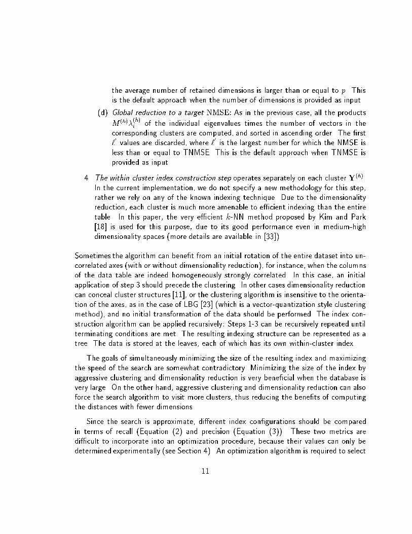
Figure 5: (a) Relation between retained volume and Normalized Mean Squared Error. The

plots are parameterized by the number of clusters. (b) Database compression as a function

of the NMSE, parameterized by the number of clusters. The cost of storing the centroids

and the dimensionality reduction information is ignored. Compression ratios of more than

60 are possible when all the dimensions of several clusters are discarded, in which case the

points are represented by the corresponding centroids. Table size: 16; 129� 60.

The relationship between the approximation induced by CSVD, measured in terms of

NMSE, and the number of retained dimensions (p), or equivalently the fraction of retained

volume (Fvol), was discussed in Section 2.2. Since SVD, and hence CSVD, is only desirable

21

if NMSE is small for high data compression ratios, we have quanti�ed experimentally this

relation.

In Figure 5(a), the percentage retained volume Fvol is plotted as a function of theNMSE. As the relation between Fvol and NMSE is a function of the number of clusters

H, the plot shows di�erent curves parameterized by di�erent values of H. The line cor-

responding to a single cluster shows the e�ects of using SVD alone without clustering.

There is a signi�cant drop in Fvol for even small values of NMSE, suggesting that few

dimensions of the transformed features capture a signi�cant portion of the variance. How-ever, the presence of local structure is quite evident: when the NMSE is equal to :1, using

32 clusters reduces the dimensionality of the search space from 60 to less than 5, whilesimple SVD retains 24 dimensions.

0 0.05 0.1 0.15 0.2 0.25 0.3 0.3510

0

101

102

Compression Improvement over SVD

Impr

ovem

ent o

ver

SV

D

NMSE

2 clusters 4 clusters 8 clusters 16 clusters 32 clusters 64 clusters 128 clusters

0 0.05 0.1 0.15 0.2 0.25 0.3 0.35

100

101

Compression Improvement over SVD, including index overhead

Impr

ovem

ent o

ver

SV

D

NMSE

2 clusters 4 clusters 8 clusters 16 clusters 32 clusters 64 clusters 128 clusters

(a) (b)

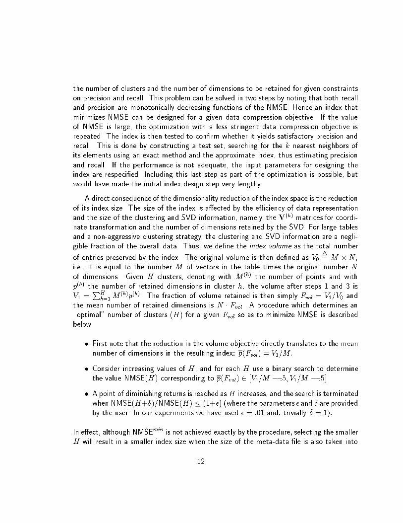
Figure 6: (a) Improvement in dimensionality reduction (compression) over simple SVD

as a function of the NMSE. (b) Improvement in index size including the clustering and

dimensionality reduction overhead. Both �gures show plots parameterized by the number

of clusters. Table size: 16; 129� 60.

The reduction in the fraction of retained volume Fvol as the NMSE grows, is an

increasing function of the number of clusters. For example, NMSE= :05 results in Fvol �

:52 for H = 1 cluster, and Fvol � :12 for H = 32 clusters, indicating that CSVD

outperforms SVD to a signi�cant extent. This con�rms the presence of local structurethat cannot be captured by a global method such as SVD.

22

Figure 5(b) shows the overall compression ratio achieved as a function of the NMSE,

parameterized by the number of clusters, computed as the ratio of the number of dimen-

sions in the search space to the average number of retained dimensions required to attain

the NMSE objective. The approach number 3d to dimensionality reduction was used to

produce the plot. Figure 6(a) shows the improvement in compression ratio over simpleSVD, as a function of NMSE. As before, the larger the number of clusters, the better

CSVD adapts to the local structure of the database, and the higher is the compression

ratio that can be achieved for the same NMSE of the reduced dimensionality index to

the original database. Note that signi�cant advantages in compression ratio over simple

SVD are attained in the interesting region :05 � NMSE � :15. If the overhead dueto the index is accounted for, the compression improvement over simple SVD is smaller,as seen in Figure 6(b). This overhead is equal to the cost of storing, for each cluster,

both the centroid and the part of the matrix V required to project the samples onto thecorresponding subspace. The �rst component is equal to H �N (the number of clusters

times the number of dimensions of the original space), and the second is equal to the

sum over all clusters of N times the number of retained dimensions. The e�ect of theoverhead is very substantial given the small database size, but are much less pronouncedin experiments based on the larger databases. While eventually the trend seen in Fig-ure 5 is reversed, as the cost of adding an additional cluster is larger than the saving

in dimensionality reduction, this e�ect is moderate for the parameter range used in theexperiments, even when the small database is used. The overhead is small for H � 16,where the overall compression ratio is reduced by a factor of 1:2 or less, and is important

only for H � 32. For H = 32 the overall compression ratio is reduced by factor of 1:1 atlow NMSE, and 1:7 at high NMSE.

A di�erent view of the same data is provided in Figure 7(a), where the �delity index (de-�ned as 1�NMSE) is plotted as a function of number of clusters and is parameterized by

the percentage of retained volume. Figure 7(b) plots the ratioNMSESV D=NMSECSV D(H),

which measure the increase in �delity to the original data, parameterized by the percent-

age of retained volume. Note that CSVD always outperforms SVD, and that there is asubstantial reduction in NMSE as the number of clusters H, for all values of Fvol con-

sidered. Similar results are obtained with even larger datasets, with over 200,000 rows

and 42 dimensions, but the optimum value for H depends on the dataset, Fvol; and thequality of the clustering method.

23

0.4

0.5

0.6

0.7

0.8

0.9

1

1 2 4 8 16 32Number of Clusters

1−N

MS

E

Fidelity vs number of clusters

50% vol 31% vol 20% vol 13% vol 9% vol 5.5% vol

100

101

Number of ClustersN

MS

E(1

) / N

MS

E(n

)

Fidelity vs number of clusters

1 2 4 8 16 32

50% vol 31% vol 20% vol 13% vol 9% vol 5.5% vol

(a) (b)

Figure 7: (a) Dependence of �delity (de�ned as 1�NMSE) on the number of clusters,

parameterized by the volume compression. (b) Increase in �delity (de�ned as the inverse

ratio of the NMSE's) over simple SVD, parameterized by the volume compression (log-log

plot). Table size: 16; 129� 60.

4.3 The E�ect of Approximate Search on Precision and Re-

call

The price paid for improving performance via dimensionality reduction is that the resultingsearch becomes approximate. Here, the source of the approximation is the projection ofthe vectors in the database onto the subspace of the corresponding cluster: the retrieval

phase is based on the (exact) distances between the query template and the projectedvectors rather than the original vectors. We de�ne the retrieval to be exact if the approx-

imation does not change the ordering of the distances between the returned records andthe query point, i.e., the original ranking of points is preserved, which is a common occur-

rence when the discarded variance is negligible. However, when the approximations due

to the projection of the database records onto the subspaces of the corresponding clustersyield larger errors, discrepancies in distance ordering occur, giving rise to erroneous rank-ings. Consequently, when issuing a k-nearest-neighbor query, some undesired records are

retrieved and some desired records are discarded. To quantify these e�ects, we can use

the recall parameter, de�ned in Equation (2). The recalls of individual queries are not a

24

0 .10 .20 .30 .40 .50 .60 .7010

20

30

40

50

60

70

80

90

100

Normalized Mean Squared Error

Pre

cisi

on (

perc

ent)

Precision as function of NMSE, recall = 90%

1 cluster 4 clusters 8 clusters 16 clusters32 clusters

0 .10 .20 .30 .40 .50 .6010

20

30

40

50

60

70

80

90

100

Normalized Mean Squared Error

Pre

cisi

on (

perc

ent)

Recall = 0.8

2 clusters 4 clusters 8 clusters16 clusters32 clusters

(a) (b)

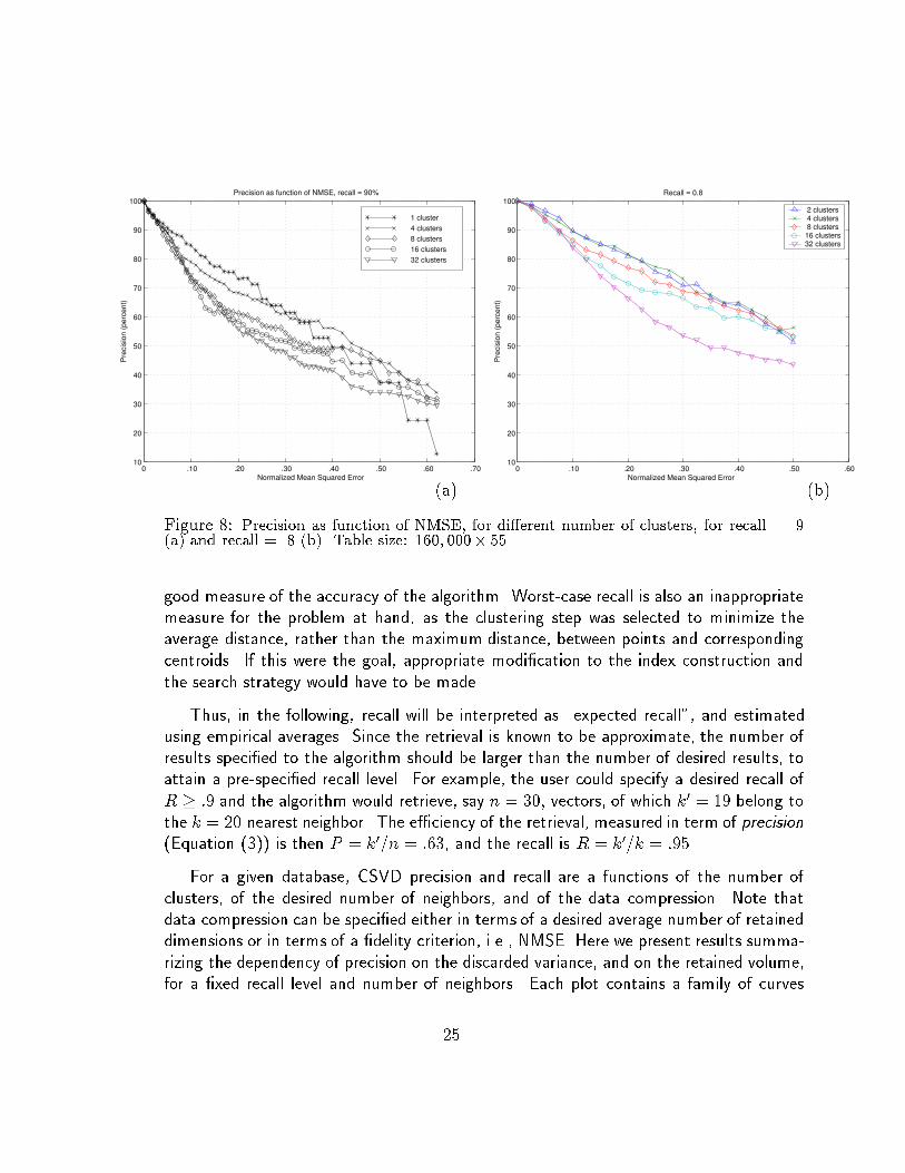
Figure 8: Precision as function of NMSE, for di�erent number of clusters, for recall = .9(a) and recall = .8 (b). Table size: 160; 000� 55.

good measure of the accuracy of the algorithm. Worst-case recall is also an inappropriatemeasure for the problem at hand, as the clustering step was selected to minimize theaverage distance, rather than the maximum distance, between points and corresponding

centroids. If this were the goal, appropriate modi�cation to the index construction and

the search strategy would have to be made.

Thus, in the following, recall will be interpreted as \expected recall", and estimatedusing empirical averages. Since the retrieval is known to be approximate, the number of

results speci�ed to the algorithm should be larger than the number of desired results, to

attain a pre-speci�ed recall level. For example, the user could specify a desired recall of

R � :9 and the algorithm would retrieve, say n = 30; vectors, of which k0 = 19 belong to

the k = 20 nearest neighbor. The e�ciency of the retrieval, measured in term of precision(Equation (3)) is then P = k

0=n = :63, and the recall is R = k

0=k = :95

For a given database, CSVD precision and recall are a functions of the number of

clusters, of the desired number of neighbors, and of the data compression. Note thatdata compression can be speci�ed either in terms of a desired average number of retained

dimensions or in terms of a �delity criterion, i.e., NMSE. Here we present results summa-

rizing the dependency of precision on the discarded variance, and on the retained volume,for a �xed recall level and number of neighbors. Each plot contains a family of curves

25

parameterized by the number of clusters.

To estimate the value of P for a speci�ed recall value (Rthreshold) and a pre-de�ned

number of neighbors k, we determine for each query point q the minimum value of n,nq, yielding k

0� k � Rthreshold correct results. Then P (q) = k

0=nq, and the expected

precision is estimated as the average of P (q) over a set of query points of the same size

as the database. Figure 8 characterizes the mean precision (P ) for k = 20 as a functionof the NMSE for various number of clusters, and for two values of recall, Rthreshold = :9,

and Rthreshold = :8 Note �rst that P > :5 for NMSE up to :4 and R = :9, and up to

10 20 30 40 50 60 70 80 90 10050

55

60

65

70

75

80

85

90

95

100

Volume (percentage)

Pre

cisi

on (

perc

enta

ge)

Precision as function of volume

1 cluster 2 clusters 4 clusters 8 clusters16 clusters 32 clusters

50 55 60 65 70 75 80 85 90 950

10

20

30

40

50

60

70

80

90

100Precision as a function of recall, 16 clusters, 20 nearest neighbors

Recall (percentage)

Pre

cisi

on

NMSE = .05 NMSE = .10NMSE = .15 NMSE = .20 NMSE = .25 NMSE = .30 NMSE = .35 NMSE = .40 NMSE = .45 NMSE = .50

(a) (b)

Figure 9: Precision as function of the retained index volume (a), for di�erent number of

clusters. Recall = :9, table size 160; 000� 55. Precision as a function of recall (b). Table

size = 16; 129� 60, number of clusters = 16, desired number of nearest neighbors = 20.

The curves are parameterized by the retained variance.

NMSE = :5 and R = :8. A single cluster provides the highest precision when NMSE is

small. This can be attributed to the inaccuracies in reconciling inter-cluster distances andresults in reduced precision (see Figure 4). Unsurprisingly, clustering reduces precision for

a given NMSE. The higher the clustering degree, the higher is the average dimensionality

reduction. Projections of points within individual clusters are much closer than they

would be if simple SVD were used, and therefore some discrimination is lost. The e�ect is

moderate for NMSE < :10, and becomes more substantial afterwards. In some occasionwe have noticed that, beyond this threshold, entire small clusters are projected onto their

26

centroid. Eventually, however, the trend is reversed, and for NMSE > :5 the precision

di�erence between CSVD and simple SVD becomes smaller. Also, in the interesting zone

NMSE < 10%, good precision values are observed across the board. The reported results

are typical of those obtained on a large number of combinations of the values of k and

Rthreshold.

Figure 9(a) shows the mean precision as a function of Fvol parameterized by the

number of clusters, with recall �xed at :9. Note that H = 32 clusters result in the highest

precision curve, and that for the same volume reduction level the best information is

preserved with a higher number of clusters. This was to be expected, since for �xed index

compression the NMSE decreases signi�cantly with the number of clusters (Figure 7),

which results in a higher precision. Finally, it is interesting to note that for 32 cluster,even when the data compression ratio is 5:1, the precision is around 80%, and when the

compression ratios is 8:1 the precision remains slightly less than 70%. In this last case,to achieve R = :9 during an k-NN search, it is enough to retrieve 1:5 k results andpost-process them to rank the results correctly.

In Figure 9(b), the precision versus recall curve parameterized by di�erent values ofNMSE. The experiment was carried out with sixteen clusters, and similar graphs can be

obtained for di�erent number of clusters. It is observed that the NMSE has the primarye�ect on precision and the e�ect of increased recall is secondary. Precision deteriorateswith increasing recall, but the drop is relatively small.

In an operational system, the empirical precision versus recall curve P (R) would bestored with the indexing structure. The speci�cation of a query consists then of providinga query point, the minimum desired expected recall Rthreshold and the desired numberof nearest neighbors k. The system would then retrieve n = k=P (Rthreshold) vectors

using CSVD, score them in the original search space, and return the top k matches. Thisprocedure yields on average the desired precision.

Alternatively, a more conservative approach would be to construct a histogram of

precision values parameterized by recall, and use a precision quantile smaller than theaverage, n = k=Pq, which would yield the desired recall 1� p of the times.

4.4 Retrieval Speedup

The main purpose of an indexing structure is to increase the retrieval speed over a linear

scan of the entire database. As reducing the number of dimensions makes it possible

to store the index to the entire databases in the main memory of a computer (current

27

4 6 8 10 12 14 16 18 200

5

10

15

20

25

30

Database size = 160k

Speedup vs. Retained Dimensions

Retained Dimensions

Spe

edup


5 10 15 20 25 300

50

100

150


Speedup vs. Retained Dimensions

Retained Dimensions

Spe

edup


(a) (b)

Figure 10: Speedup as a function of retained dimensions for texture feature databases con-

taining (a) 16,129 60-dimensional entries and (b) 160,000 55-dimensional entries. Note that

here the line corresponding to 1 cluster depicts the e�ects of simple SVD+dimensionality

reduction, where the maximum observed speedup is about 10.

small and mid-range database servers have gigabytes of primary store, and very largememories are becoming increasingly pervasive), it is important to quantify the in-memory

performance of the index. The comparison is performed with respect to sequential scan,

rather than with respect to other indexes. As it is relatively simple to implement verye�cient versions of sequential scan using highly optimized native routines, it can be

universally used as baseline for every indexing method. On the contrary, to perform a faircomparison, competing indexing structures would have to be recoded and optimized for

the speci�c architecture on which the test is run.

Figure 10 shows the behavior of the speedup as a function of the number of retaineddimensions. The search was for the 20 nearest neighbors of the query template. The

number of actually retrieved neighbors was selected to ensure a minimumaverage recall of:9, and therefore varies with the number of clusters and the number of retained dimensions.

Note that, for indexes with 32 clusters, the observed speedups in the smaller database

ranged between 15 and 30, while for the larger database the observed speedups are �ve

times larger, thus showing that, within the range of database sizes used, the index scaleswith the number of samples in the table.

28

0.955 0.96 0.965 0.97 0.975 0.98 0.985 0.99 0.995 10

5

10

15

20

25

30

Recall

Spe

edup

Speedup vs. Recall

Database size = 16k

2 clusters 4 clusters 8 clusters 16 clusters32 clusters

0.85 0.9 0.95 10

50

100

150

Recall

Spe

edup

Speedup vs. Recall


2 clusters 4 clusters 8 clusters 16 clusters32 clusters

(a) (b)

Figure 11: Speedup as a function of recall, for texture feature databases containing (a)

16,129 60-dimensional entries and (b) 160,000 55-dimensional entries.

A di�erent view of the data is obtained by plotting the speedup as a function of the

average recall, as shown in Figure 11. Note how in the 32 cluster case, and for the larger

database, speedups of 140 are observed while maintaining 96% recall on a 20 nearestneighbor search, which implies that on average 19 of the 20 desired results were retrieved.The recall can be improved to 97:5% while still achieving 130 fold speedup: here morethan half of the 100,000 queries corresponding to each point in the graph returned all

the desired 20 nearest neighbors. It is also interesting to note how in this case the �ne

structure of the data is better suited to a larger number of clusters.

4.5 CSVD and within-cluster indexing

As discussed in Section 3.4, the increase in search speed is due to both CSVD and itse�ects on the within-cluster search index. In this section, we quantify the contributions

of these e�ects, using experiments based on the larger of the data sets.

In the �rst set of experiments, the test query returns the 20 nearest neighbors of the

template. The recall level is �xed to be between :95 and :96, thus, on average, at least 19of the 20 results are correct. To obtain the desired recall, the number of actually retrieved

29

2 4 8 16 320

10

20

30

40

50

60

70

80

90

100

number of clusters

% d

b in

touc

hed

clus

ters

Percentage of db contained in touched clusters

nn =20, .95 < recall < .96

p=30p=20 p=10

2 4 8 16 320

5

10

15

20

25

30

35

40

45

50

number of clustersS

peed

up d

ue to

CS

VD

alo

ne

Speedup due to CSVD vs number of clusters

nn =20, .95 < recall < .96

Dim = 55, DB size = 160K

p=30p=20 p=10

(a) (b)

Figure 12: (a) The percentage of the database in the touched clusters. (b) The increase in

retrieval speed (b) due to CSVD alone. Both quantities plotted as a function of the number

of retained dimensions and of the number of clusters. Table size =56; 688� 60.

samples is selected to yield the correct point of the precision-vs-recall curve (Figure 9(b))computed for the desired number of clusters. Additional diagnostic code is enabled, which

records the average number of visited clusters, the average number of visited terminalnodes and the average number of non-terminal visited nodes. The diagnostic code has aside e�ect of slightly reducing the observed speedup, thus the results shown in this section

are slightly worse than those shown in previous sections. Each data point corresponds tothe average of 80,000 retrievals (10,000 retrievals for each of 8 indexes).

Recall that the average increase in retrieval speed due to CSVD alone (i.e., when

the within-cluster search is exhaustive) is roughly equal to the index compression ratio

times the expected ratio of the database size to the number of elements contained in

the clusters visited during the search. Figure 12(a) shows the average percentage of thedatabase contained in the visited clusters, as a function of the overall number of clusters

in the index, and parameterized by the number of retained dimensions. The number ofclusters in the index has the largest e�ect on the percentage of the database visited during

queries. We have observed that, when the index contains 2 clusters, both are searched

during more than 90% of the queries; when the index contains 8 clusters, slightly less

than half of them are visited on average, while when the index contains 32 clusters, only

30

2 4 8 16 320

20

40

60

80

100

120

140

160

180

number of clusters

spee

dup

nn =20, .95 < recall < .96


Observed speedup as a function of clusters and dimensions

p=30p=20 p=10

2 4 8 16 320

5

10

15

20

25

30

number of clusterssp

eedu

p

nn =20, .95 < recall < .96


Additional speedup due to within−cluster indexing

p=30p=20 p=10

(a) (b)

Figure 13: (a) The observed speedup; (b) the additional speedup due to within-cluster

indexing; both quantities plotted as a function of the number of retained dimensions p and

of the number of clusters. Table size =56; 688� 60.

three are searched on average. An important consequence is the following: If the clustercontents were paged and read from disk during query processing, using SVD would require

loading the entire database each time. When the index contains 32 clusters, on averageonly 10% of the database would be read from tertiary storage in response to a query. Fromthe �gure, we also note that the e�ect of the number of retained dimensions is secondary:in CSVD the selection of the primary cluster and of the candidates is performed in the

original data space, and it is therefore not signi�cantly a�ected by the within-clusterdimensionality reduction. However, the dimensionality reduction has a direct e�ect on the

precision-recall curve (Figure 9(b)), and, to achieve the desired 95% recall, the numberof retrieved samples increases with the number of discarded dimensions, thus resulting in

a slightly larger average number of visited clusters and a slightly higher curve for smaller

number of retained dimensions.

Figure 12(b) displays the expected speedup over linear scan under the assumption that

each of the visited clusters is exhaustively searched. In the �gure, the additional costs

of projecting the query vector, of identifying the primary and candidate clusters, and of

maintaining the list of partial results, are ignored. Here, the dimensionality reduction plays

a major role, as it controls the data volume to be read from memory to the processor and

31

the number of oating point operations required to compute distances.

Figure 13(a) shows the actually observed speedup when using within-cluster indexing,

which also includes the costs of searching CSVD and of maintaining the list of partialresults. The data points in the �gures were obtained with the Kim-Park index, by requiring

a minimumfan-out of 4 for internal nodes, and a minimumnumber of points per leaf equal

to 4. These observed values are larger than the corresponding ones in Figure 12(b) by thefactor depicted in Figure 13(b). Recall that, for generic high-dimensional feature space, we

would expect the within-cluster index to have some moderate e�ect in 10 dimensions, but

to be essentially useless in 20 or more dimensions. The experimental evidence, however,contradicts this intuition. When 30 or 10 dimensions are retained, the dependence on the

number of clusters is moderate, and the e�ect of the indexing is an increase in speed ofaround 10 and 3 respectively. In 20 dimensions, the increase in speed is rather dramatic,ranging from 18 to 28 times for H > 2.

We conclude that CSVD transforms the data in a form that is well suited for use with

some multidimensional indexing, in particular with recursive partitioning methods thatsplit the space using hyperplanes perpendicular to the coordinate axes, that split acrossone coordinate at a time, and that can either select the dimensions for partitioning or

that partition them in a round robin fashion.

4.6 Within-cluster indexing design

The within-cluster search cost can be divided into two components: walking the tree toidentify candidate leaves, and exhaustively searching the leaves. We include the cost of

maintaining the list of current candidates in the �rst component.

When the entire index is in main memory, the cost of exhaustively searching leaves

is essentially determined by the CPU, provided that the implementation of the distancecomputation algorithm makes good use of the memory hierarchy. Figure 14(a) showsthe relative computational costs of visiting the tree and the leaf nodes recorded in the

experiments used to construct Figures 12 and 13. It is immediately clear that decreasing

the number of retained dimensions increases the cost of visiting the tree. This is notsurprising: the cost of exhaustively searching a leaf is directly proportional to the lengthof each contained vector. If this were the only e�ect, the relative cost of searching the

leaves in 20 and 30 dimensions would be less than twice and three times, respectively, the

cost of searching the leaves in 10 dimensions. The �gure, however, suggests the presence

of secondary e�ects, which increase these relative costs. The Kim-Park tree is used to

32

4 8 16 32 5.50

0.1

0.2

0.3

0.4

0.5

0.6

0.7

0.8

0.9

1Dim 30 30 30 3020 20 20 2010 10 10 10

Term

inal S

earchT

ree Search

number of clusters

prop

ortio

n of

tim

e

Relative Costs of Tree Traversal and Terminal Bucket Search

2 4 8 16 320

1

2

3

4

5

6

7

8

number of clusters%

of d

b in

vis

ited

buck

ets

percentage of db in visited buckets, vs number of clusters

nn =20, .95< recall < .96

p= 30p=20 p=10

(a) (b)

Figure 14: (a) Relative costs of tree and terminal bucket search. (b) Average percentage

of the database in the exhaustively searched terminal bins, parameterized by the number

of retained dimensions p. Table size =160; 000� 55, within-cluster index fanout = 4, leaf

size = 4; Desired number of nearest neighbors = 20, actual number of retrieved samples

adjusted to maintain Recall between :95 and :96

index only the �rst few dimensions (from 4 to 8, depending on the number of clusters),

that contribute to a large part of the variability of the data. Candidate nodes and leaves

are therefore determined in 4- to 8-dimensional spaces, while distances between the queryand the vectors stored at the leaves are computed in 10, 20 or 30 dimensions. Due to

this di�erence, the number of candidate nodes visited during the search increases withthe retained number of dimensions. We shall see immediately that most of the additionalcandidates are internal nodes rather than leaves.

When the leaf nodes are stored on disk, and cached only when required, the searchcost is essentially determined by the I/O, and the speedup with respect to exhaustive scan

of the entire database is essentially equal to the reciprocal of the fraction of the databasecontained in the visited leaves. This last quantity is shown, as a percentage, Figure 14(b).

Note, �rst, that the number of retained dimensions has a secondary e�ect, indicating that

the number of visited leaves does not change signi�cantly with the number of retaineddimensions. The number of clusters, however, has a major e�ect. For example, whenretaining 20 dimensions on average, a CSVD index based on 2 clusters visits on average

33

7% of the database in response to a query, while an index based on 32 clusters visits on

average :7% of the database, which corresponds to a 10-fold gain.

2 3 4 5 6 7 8 90

0.5

1

1.5

2

2.5

3

3.5

4

4.5

5

Minimum number of splits

Spe

edup

(cl

uste

r in

dexi

ng o

nly)

Speedup vs number of splits

Database size = 56644

Nr. features = 60

Number of nn = 80

p=30 Bucket=32p=20 Bucket=32p=10 Bucket=32p=30 Bucket=64p=20 Bucket=64p=10 Bucket=64

0 10 20 30 40 50 60 70 80 90 1000

0.5

1

1.5

2

2.5

3

3.5

4

4.5

5

5.5

Size of terminal bucket

Spe

edup

(cl

uste

r in

dexi

ng o

nly)

Speedup vs Terminal Bucket Size

Database size = 56644Nr. features = 60Number of nn = 80Nr. clusters = 16

Splits = 5Splits = 6Splits = 7

(a) (b)

Figure 15: (a) Speedup due to within cluster index as a function of fanout, parameterized

by the number of retained dimensions p and the bucket size; (b) Speedup due to within

cluster index as a function of the terminal bucket size, parameterized by the fanout, for 16

clusters. Table size =56; 688�60, desired number of nearest neighbors = 80, actual number

of retrieved samples adjusted to maintain Recall between :95 and :96

Additional design points are the size of the terminal leaves and the desired fan-out atinternal nodes. We have found that leave sizes between 32 and 64 combined with fan-outbetween 4 and 6 produce the best results on our databases (Figure 15).

5 Summary

Many emerging multimedia database and data mining applications require e�cient sim-ilarity retrieval techniques from very high dimensional datasets. In this paper, a novel

methodology, Clustering Singular Value Decomposition (CSVD), is proposed for approxi-

mate indexing of numeric tables with high dimensionality. This method achieves additional

dimensionality reduction than those based on SVD for a �xed NMSE by exploiting thelocal structure of heterogeneous datasets. In the proposed method, the feature space is

34

�rst partitioned into multiple subspaces and a dimension reduction technique such as SVD

is then applied to each subspace. The CSVD index is constructed by recording the cen-

troid of each cluster, the cluster radius, and its projection matrix. Search is performed by

alternating the identi�cation of the best unsearched candidate cluster to a within-cluster

search step, until no candidate remain. A cluster is a candidate if it can contain samplesthat are closer to the query template than some of the currently retrieved results. Candi-

date clusters are identi�ed with a simple but fast method requiring only the computation

of the squared distance between query template and cluster centroid (computed at query-

execution time) and of the squared radius of the cluster (computed while constructing the

index).

Within-cluster search is performed on reduced dimensionality versions of the querytemplate and cluster data-points, using an existing indexing structure and correcting forthe distance between the query sample and the cluster subspace. Since SVD sorts the

dimensions of the rotated space in order of decreasing variance, the indexing can be limitedto the �rst few dimensions whenever they capture a signi�cant portion of the variability.

The e�ectiveness of the proposed CSVD method is validated with datasets consistingof feature vectors extracted from three benchmark databases containing feature vectors

extracted from remotely sensed images. With similar precision vs. recall performance,it is shown in this paper that the CSVD method has a signi�cantly better �delity tothe original data than SVD for a 20-fold dimensionality reduction. Conversely, for �xedvalues of NMSE, search using CSVD signi�cantly faster than linear scan, especially asthe database size grows. For moderate size databases containing 160,000 55-dimensional

records, we have observed an 140-fold increase in speed while maintaining a recall ofbetter than 95% when retrieving 20 nearest neighbors.

Several other dimensions of the index design have been explored in the paper, such asthe selection of the number of actually retrieved results to ensure a desired recall value,

and the dependence of the speed on the within-cluster index parameters.

Several extensions to this work are currently in progress, in particular we are exploringthe performance of SVD-friendly clustering methods, i.e., methods that create clusters

with an eye on reduced dimensionality. We are also investigating the e�ect of multi-level

clustering and SVD on performance and develop procedures for constructing an optimal

index in this case.

35

Acknowledgements

We would like to wholeheartedly thank Dr. Philip S. Yu and Dr. Charu C. Aggarwal for the

insightful discussions, precious suggestions, useful references and for their encouragement.

We would also like to thank an anonymous Japanese patent examiner for pointing us to

the essential reference [35].

This work was funded in part by grant no. NASA/CAN NCC5-101.

References

[1] C.C. Aggarwal and P.S. Yu. Finding generalized projected clusters in high dimensionalspaces. In Proc. 2000 ACM SIGMOD Int'l Conf. on Management of Data, page To

appear, May 14{19 2000.

[2] M. Beatty and B.S. Manjunath. Dimensionality reduction using multi-dimensional

scaling for content-based retrieval. In Proc. IEEE Int'l Conf. Image Processing,ICIP '97, volume 2, pages 835{838, Santa Barbara, CA, October 1997.

[3] N. Beckmann, H.P. Kriegel, R. Shneider, and B. Seeker. The R��tree: an e�cient

and robust access method for points and rectangles. In Proc. 1990 ACM SIGMODInt'l Conf. on Management of Data, pages 322{331, Atlantic City, NJ, USA, May23-25 1990.

[4] S. Berchtold, C. Bohm, B. Braunmueller, D.A. Keim, and H.-P. Kriegel. Fast parallelsimilarity search in multimedia databases. In Proc. 1997 ACM SIGMOD Int'l Conf.on Management of Data, pages 1{12, Tucson, AZ, 12-15 May 1997.

[5] S. Berchtold, C. Bohm, D.A. Keim, and H.-P. Kriegel. A cost model for nearestneighbor search in high-dimensional data space. In Proc. 16th ACM ACM Symp.

Principles of Database Systems, PODS '97, pages 78{86, Tucson, AZ, May 1997.

[6] S. Berchtold, D.A. Keim, and H.-P. Kriegel. The X-tree: An index structure for high-dimensional data. In Proc. 19th Int'l Conf. on Very Large Data Bases VLDB '93,

pages 28{39, Bombay, India, September 1996.

[7] K. Beyer, J. Goldstein, R. Ramakrishnan, and U. Shaft. When is \nearest neighbor"

meaningful? In Proc. Int'l Conf. Database Theory (ICDT '99), pages 217{235,

Jerusalem, Israel, 1999.

36

[8] S. Blott and R. Weber. A simple vector-approximation �le for similarity search in

high-dimensional vector spaces. Technical report, Institute of Information Systems,

ETH, Zurich, Switzerland, 1997.

[9] V.S. Cherkassky, J.H. Friedman, and H. Wechsler. From Statistics To Neural Net-

works: Theory and Pattern Recognition Applications. Springer-Verlag, 1993.

[10] A.P. Dempster, N.M. Laird, and D.B. Rubin. Maximum likelihood from incompletedata via the EM algorithm. J. Royal Statistical Soc. B, 39(1):1{38, 1977.

[11] B.S. Everitt. Cluster Analysis. John Wiley & Sons, 3rd edition, 1993.

[12] C. Faloutsos. Searching Multimedia Databases by Content. Kluwer Academic Pub-lishers, Boston, 1996.

[13] C. Faloutsos and K.-I. Lin. FastMap: a fast algorithm for indexing, data-mining, and

visualization of traditional and multimedia datasets. In Proc. 1995 ACM SIGMODInt'l Conf. on Management of Data, pages 163{174, San Jose, CA, May 1995.

[14] B.V. Gaede and O. Gunther. Mutidimensional access methods. ACM ComputingSurveys, 30(2):170{231, June 1998.

[15] A. Guttman. R-trees: a dynamic index structure for spatial searching. ACM SIGMOD

Record, 14(2):47{57, June 1984.

[16] T.Y. Hou, P. Liu, A. Hsu, and M.Y. Chiu. Medical image retrieval by spatial feature.

In Proc IEEE Int'l Conf. Systems, Man, and Cybernetics, pages 1364{1369, 1992.

[17] I.T. Jolli�e. Principal Component Analysis. Springer-Verlag, New York, 1986.

[18] B.S. Kim and S.B. Park. A fast k nearest neighbor �nding algorithm based on the

ordered partition. IEEE Trans. Pattern Analysis and Machine Intelligence, PAMI-

8(6):761{766, November 1986.

[19] F. Korn, H.V. Jagadish, and C. Faloutsos. E�ciently supporting ad hoc queries

in large datasets of time sequences. In Proc. 1997 ACM SIGMOD Int'l Conf. onManagement of Data, pages 289{300, Tucson, AZ, May 1997.

[20] R. Kurniawatio, J.S. Jin, and J.A. Shepherd. The SS+-tree: An improved indexstructure for similarity searches. In Proc. SPIE - Int. Soc. Opt. Eng., volume 3022,

Storage Retrieval Image Video Databases V, pages 110{120, February 1997.

37

[21] C.-S. Li and V. Castelli. Deriving texture feature set for content-based retrieval

of satellite image database. In Proc. of the IEEE Int'l Conf. Image Proc., pages

567{579, Santa Barbara, CA, Oct. 26-29 1997.

[22] C.-S. Li, V. Castelli, and L.D. Bergman. Progressive content-based retrieval from

distributed image/video databases. In Proc. 1997 IEEE Int'l Symp. Circuit Systems

ISCAS97, volume 2, pages 1484{87, Hong Kong, June 9-12 1997.

[23] Y. Linde, A. Buzo, and R.M. Gray. An algorithm for vector quantizer design. IEEE

Trans. Communications, COM-28(1):84{95, January 1980.

[24] A. Pentland, R.W. Picard, and S. Sclaro�. Photobook: Tools for content-based

manipulation of image databases. In Proc. SPIE - Int. Soc. Opt. Eng., volume 2185,Storage Retrieval Image Video Databases, pages 34{47, February 1994.

[25] L. M. Po and C. K. Chan. Tree search structures for image vector quantization. InProc. of Int'l Symposium Sig. Proc. and Appl. ISSPA 90, volume 2, pages 527{530,Australia, August 1990.

[26] W.H. Press, S.A. Teukolsky, W.T. Vetterling, and B.P. Flannery. Numerical Recipesin C. Prentice-Hall, 1993.

[27] J.T. Robinson. The k-d-b-tree: A search structure for large multidimensional dynamicindexes. In Proc. 1981 ACM SIGMOD Int'l Conf. on Management of Data, pages10{18, 1981.

[28] N. Russopoulos, S. Kelley, and F. Vincent. Narest neighbor queries. In Proc. 1995ACM SIGMOD Int'l Conf. on Management of Data, pages 71{79, San Jose, CA,

May 1995.

[29] R. Samadani, C. Han, and L.K. Katragadda. Content-based event selection fromsatellite images of the aurora. In Proc. SPIE - Int. Soc. Opt. Eng., volume 1908,

Storage Retriev. Image Video Datab., pages 50{59, February 1993.

[30] J.R. Smith and S.-F. Chang. VisualSeek: A fully automated content-based image

query system. In Proc. ACM Multimedia '96, pages 87{98, Boston, MA, USA, Nov.

18-22 1996.

[31] T.R. Smith. A digital library for geographically referenced materials. IEEE Computer

Magazine, 29(5):54{60, May 1996.

38

[32] S. W. Smoliar and H. Zhang. Content based video indexing and retrieval. IEEE

Multimedia, 1(2):62{72, Summer 1994.

[33] A. Thomasian, V. Castelli, and C.-S. Li. RCSVD: Recursive clustering with singu-

lar value decomposition for dimension reduction in content-based retrieval of largeimage/video databases. Research Report RC 20704, IBM, 01/28/1997.

[34] W. Niblack et al. The QBIC project: Querying images by content using color texture,

and shape. In Proc. SPIE - Int. Soc. Opt. Eng., volume 1908, Storage Retrieval Image

Video Databases, pages 173{187, 1993.

[35] Y.T. Young and P.S. Liu. Overhead storage consideration in a multilinear methodfor data �le compression. IEEE Trans. Software Engineering, SE-6(4):340{347, July1980.

A A Property of PCA

It is known that PCA minimizes the normalized root mean square error metric (NRMSE),among all procedures consisting of a linear transformation followed by variable subset

selection. Here, the NRMSE is de�ned as [19]

NRMSE =

qPM

i=1

PN

i=1(xi;j � x0i;j)2

qPM

i=1

PN

j=1(xi;j ��j)2: (8)

In this equation (xi;j � x0i;j)

2 is the squared error for the (i; j)th row of the matrix, x0i;jis the approximation to xi;j value given by Equation (11) below, and � is the centroid

of the collection of points. Thus, the numerator is the overall squared error introduced

by the approximation. The denominator is the mean distance squared from the points tothe centroid of the corresponding cluster times the number of points M . The NRMSE

2

is therefore the fraction of the total variance lost to dimensionality reduction, and, usingthe notation of Section 2.2 can be expressed as NRMSE

2 = 1� Fvar: In the following,

assume without loss of generality that � is the origin of the coordinate axes.

When performing dimensionality reduction following SVD, the p columns of the column-orthonormal matrix U corresponding to the highest eigenvalues are retained [19].

The matrix U is obtained directly from Eq. (4). However, if eigenvalues and eigen-vectors are obtained by decomposing the covariance matrix as C = V�V

T , (Equation

39

(5)) thenU can be computed from the original data as U = XVS�1, by post-multiplying

Equation (4) with VS�1.

For a given number of retained dimensions p both methods introduce the same error

as shown below. The method given in this paper is more e�cient from the viewpoint of

computational cost for NN queries, window queries, etc. In the case of NN queries, once

the input or query vector is transformed and the appropriate p dimensions are selected, we

need only be concerned with these dimensions. This is less costly than applying the inverse

transformation in Eq. (4) to all the points considered by NN queries and evaluating Eq.

(1) with N dimensions. A shortcut is possible in both cases by considering the squares

of Euclidean distances and ignoring the remaining steps of a summation where the partialsum exceeds the squared distance of the kth nearest neighbor.

To show that preserving p columns of the Y matrix results in the same NRMSE and

Fvar as preserving the same dimsensions of the U matrix.

Retaining the �rst p dimensions in the transformed matrix Y = XV

yi;j =

NXk=1

xi;kvk;j; 1 � j � p; 1 � i �M: (9)

while the rest of the columns of the matrix are set to the mean and are e�ectively ignored.

The squared error in representing vector xi with yi is then

ei =

nXj=p+1

y2i;j=

nXj=p+1

nXk=1

(xi;kvk;j)2; 1 � i �M: (10)

When p dimensions of the U matrix are retained, the elements of X are approximated

by truncating the summation to p terms

x0i;j =

pXk=1

skui;kvj;k; 1 � j � N; 1 � i �M: (11)

Then the squared error in representing the ith point, given yi;m = smui;m; is

e0i =

NXj=1

NXk=p+1

(skui;kvj;k)2 =

NXj=1

NXk=p+1

(yi;kvj;k)2

40

The following few steps show that ei = e0i; 1 � i �M

NXj=1

(

NXk=p+1

yi;kvj;k)(

NXk0=p+1

yi;kvj; k) =

NXk=p+1

NXk0=p+1

yi;kyi;k0

NXj=1

vj;kvj;k0 =

NXk=p+1

NXk0=p+1

yi;kyi;k0

nXj=1

�k;k0 =

NXk=p+1

(yi;j)2 =

NXk0=p+1

NXk=1

(xi;kvk;j)2 = ei:

Note that �k;k0 = 1 for k = k0 and �k;k0 = 0 for k 6= k

0:

41

RC 21755 (98001) 30 Ma y2000 Researc h Rep ort -...

Documents

Transcript of RC 21755 (98001) 30 Ma y2000 Researc h Rep ort -...