RAVEN, a New Software for Dynamic Risk Analysis Documents/Papers/RAVEN_new_softwar… ·...
14
Probabilistic Safety Assessment and Management PSAM 12, June 2014, Honolulu, Hawaii RAVEN, a New Software for Dynamic Risk Analysis C. Rabiti a , A. Alfonsi a , J. Cogliati a , D. Mandelli a , R. Kinoshita a a Idaho National Laboratory, Idaho Falls, USA Abstract: RAVEN is a generic software driver to perform parametric and probabilistic analysis of code simulating complex systems. Initially developed to provide dynamic risk analysis capabilities to the RELAP-7 code, [1] RAVEN capabilities are currently being extended by adding Application Programming Interfaces (APIs). These interfaces are used to allow RAVEN to interface with any code as long as all the parameters that need to be perturbed are accessible by inputs files or directly via python interfaces. RAVEN is capable to investigate the system response, probing the input space using Monte Carlo, Grid strategies, or Latin Hyper Cube schemes, but its strength is its focus toward system feature discovery, such as limit surfaces, separating regions of the input space leading to system failure, using dynamic supervised learning techniques. The paper will present an overview of the software capabilities and their implementation schemes followed by some application examples. Keywords: PRA, Limit Surface, Reliability. 1. INTRODUCTION 1.1. Project Background The RAVEN [2-4] project was started at the beginning of 2012 to provide a modern framework for risk evaluation for Nuclear Power Plant (NPPs). RAVEN, under the support of the Nuclear Energy Advanced Modelling and Simulation (NEAMS) program, has been tasked to provide the necessary software and algorithmic tools to enable the application of the conceptual framework developed by the Risk Informed Safety Margin Characterization (RISMC) path-lead [5]. RISMC is one of the paths defined under the Light Water Reactor Sustainability (LWRS) DOE program. In its initial stage of development RAVEN has focused and optimized for the RELAP-7 code, currently under development at Idaho National Laboratory as future replacement of the RELAP5-3D [6] code. Since most of the capabilities developed under the RAVEN project for RELAP-7 are easily deployable to other software, currently side activities are on going for coupling RAVEN with other codes such as RELAP5-3D and BISON (fuel performance code) [7]. This paper focuses on the description of the software infrastructure and the current capabilities that are available to any generic code. 1.2. Software Goals Before starting a more deep exploration of the software capabilities and their implementations it would be helpful to review in more detail the tasks that the project was designed to accomplish. RAVEN is essentially designed as a discovery environment to characterize system responses and, in particular, to compute the risk connected to the operation of a particular system. Risk is obviously defined following the engineering approach by: =∫∫ (̅, )(̅, ) 0 ̅ . Where: ̅ : vector of the system coordinates in the phase space : time 0 : initial time (̅, )̅ : probability of the system being in ̅ , centred in ̅ , at a time within , centred in : support of (̅, )
Transcript of RAVEN, a New Software for Dynamic Risk Analysis Documents/Papers/RAVEN_new_softwar… ·...

Probabilistic Safety Assessment and Management PSAM 12, June 2014, Honolulu, Hawaii
RAVEN, a New Software for Dynamic Risk Analysis
C. Rabiti
a, A. Alfonsi
a, J. Cogliati
a, D. Mandelli
a, R. Kinoshita
a
a Idaho National Laboratory, Idaho Falls, USA
Abstract: RAVEN is a generic software driver to perform parametric and probabilistic analysis of
code simulating complex systems. Initially developed to provide dynamic risk analysis capabilities to
the RELAP-7 code, [1] RAVEN capabilities are currently being extended by adding Application
Programming Interfaces (APIs). These interfaces are used to allow RAVEN to interface with any code
as long as all the parameters that need to be perturbed are accessible by inputs files or directly via
python interfaces. RAVEN is capable to investigate the system response, probing the input space using
Monte Carlo, Grid strategies, or Latin Hyper Cube schemes, but its strength is its focus toward system
feature discovery, such as limit surfaces, separating regions of the input space leading to system
failure, using dynamic supervised learning techniques. The paper will present an overview of the
software capabilities and their implementation schemes followed by some application examples.
Keywords: PRA, Limit Surface, Reliability.
1. INTRODUCTION
1.1. Project Background
The RAVEN [2-4] project was started at the beginning of 2012 to provide a modern framework for
risk evaluation for Nuclear Power Plant (NPPs). RAVEN, under the support of the Nuclear Energy
Advanced Modelling and Simulation (NEAMS) program, has been tasked to provide the necessary
software and algorithmic tools to enable the application of the conceptual framework developed by the
Risk Informed Safety Margin Characterization (RISMC) path-lead [5]. RISMC is one of the paths
defined under the Light Water Reactor Sustainability (LWRS) DOE program. In its initial stage of
development RAVEN has focused and optimized for the RELAP-7 code, currently under development
at Idaho National Laboratory as future replacement of the RELAP5-3D [6] code. Since most of the
capabilities developed under the RAVEN project for RELAP-7 are easily deployable to other
software, currently side activities are on going for coupling RAVEN with other codes such as
RELAP5-3D and BISON (fuel performance code) [7]. This paper focuses on the description of the
software infrastructure and the current capabilities that are available to any generic code.
1.2. Software Goals
Before starting a more deep exploration of the software capabilities and their implementations it would
be helpful to review in more detail the tasks that the project was designed to accomplish. RAVEN is
essentially designed as a discovery environment to characterize system responses and, in particular, to
compute the risk connected to the operation of a particular system. Risk is obviously defined following
the engineering approach by:
𝑅 = ∫ ∫ 𝐶(�̅�, 𝑡)𝑝𝑑𝑓(�̅�, 𝑡)𝑑𝑡𝑡𝑒𝑛𝑑
𝑡0
𝑑�̅�
𝑋
.
Where:
�̅�: vector of the system coordinates in the phase space
𝑡: time
𝑡0: initial time
𝑝𝑑𝑓(�̅�, 𝑡)𝑑𝑡𝑑�̅�: probability of the system being in 𝑑�̅�, centred in �̅�, at a time within 𝑑𝑡, centred in
𝑡 𝑋: support of 𝑝𝑑𝑓(�̅�, 𝑡)

Probabilistic Safety Assessment and Management PSAM 12, June 2014, Honolulu, Hawaii
𝐶(�̅�, 𝑡): cost function
The analysis of risk, defined above, is meaningful for systems for which it is not possible to build a
fully deterministic representation and here referred as dynamic stochastic systems. Unfortunately,
these represent most of the systems of practical interest in engineering. The stochastic behaviours, or
impossibility of defining a fully deterministic model, is imposed by uncertainties in the initial
conditions, in the parameters characterizing the mathematical models used to simulate the system and
by intrinsically stochastic laws, characterizing the underlining physics.
Given that, an analysis code such as RAVEN aims to investigate the probability of the system to be
located within a certain region of the phase space. This is a classical task that could be accomplished,
for example, using the Monte Carlo (MC) method. MC is, unfortunately, notoriously computationally
expensive and therefore other sampling strategies have been and will be implemented in RAVEN.
While the evaluation of the risk is per se a relevant task, it is even more important to map the
behaviour of the risk as a function of the initial condition and of the parameters characterizing the
system behaviour (input space). The knowledge of the relationship among risk, initial conditions and
model parameters guides engineers improving the systems, prioritize additional experiments to reduce
uncertainty on selected parameters, and the development of more accurate models. RAVEN uses its
sampling methodologies to support the engineer in investigating such relationships, in a fast and
focused fashion.
2. THE SOFWARE
2.1 The Basic Elements
RAVEN is coded in Python and has a highly object oriented design. The framework can be described
through few (not all) key basic objects. A list of these objects and a summary of their most important
functionalities is reported as follows:
Distribution: In order to produce sampling of the input parameters and initial conditions, RAVEN
requires the capability to sample the possible values, based on their probabilistic distribution. In
this respect, a large library of probability distribution functions is available.
Sampler: A proper strategy to sample the input space is fundamental to the optimization of the
computational time. A sampler, in the RAVEN framework, connects a set of variables to their
corresponding distributions and produces a sequence of points in the input space.
Model: A model owns the representation of the physical system; it is therefore capable to predict
the (or one of the possible) evolution of the system given a coordinate set in the input space.
Surrogate Models (SM): As already mentioned the construction of the risk variation, as a function
of the coordinates in the input space, is a very expensive process, especially when brute force
approaches, i.e. Monte Carlo methods, are used. Surrogate models are used to speed up this
process by reducing the number of needed points and prioritizing the area of the input space to be
explored.
In addition to the ones already mentioned, there are others important entities (objects) in the RAVEN
framework but they are more closely related to the software infrastructure and therefore less important
in the illustration of the analysis capabilities of the RAVEN code.
2.2. Distribution
As already mentioned, the capability to properly represent variability in the input space is tied into the
availability of the proper probabilistic distributions. RAVEN implements an interface to the Boost
library [8] that makes available the following univariate distributions: Bernoulli, Binomial,
Exponential, Logistic, Lognormal, Normal, Poisson, Triangular, Uniform, Weibull, Gamma, and Beta.
All distributions are also available in their truncated form when this is mathematically feasible. Figure
1 shows a scattered plot of a Lognormal, normal and uniform distributions obtained with an equally
probable spaced grid with respect to the sampled parameters.
Since these distributions will be used also later on to illustrate some of the sampling strategies, for
convenience, the equations are here reported with the value of the parameters used:
𝑁𝑜𝑟𝑚𝑎𝑙(𝑥; 𝜎 = 0.5, 𝜇 = 0) = 𝑁(𝑥; 𝜎 = 0.5, 𝜇 = 0) =1
𝜎√2𝜋𝑒−(𝑥−𝜇)2
2𝜎2 ,

Probabilistic Safety Assessment and Management PSAM 12, June 2014, Honolulu, Hawaii
𝐿𝑜𝑔𝑛𝑜𝑟𝑚𝑎𝑙(𝑥; 𝜎 = 0.5, 𝜇 = 0) = 𝐿𝑁(𝑥; 𝜎 = 0.6, 𝜇 = 0) =1
𝑥𝜎√2𝜋𝑒−(𝑙𝑛(𝑥)−𝜇)2
2𝜎2 ,
𝑈𝑛𝑖𝑓𝑜𝑟𝑚(𝑥;𝑚𝑖𝑛 = 0,𝑚𝑎𝑥 = 3) = 𝑈(𝑥;𝑚𝑖𝑛 = 0,𝑚𝑎𝑥 = 3) =[𝐻(𝑥) − 𝐻(3 − 𝑥)]
3.
Figure 1: Scattered plot generated by sampling (Latin Hypercube sampling scheme) of a Normal (red),
Lognormal (blue) and Uniform distributions (green).
Many times, parameters that need to be sampled are subject to correlations. This is the case, for
example, when the same experimental setting is used to measure more physical parameters that are
then incorporated in the mathematical models. In this case it is possible that experimentalist might
suggest that the error on those parameters is correlated by, for example, a common type of dispersion.
In case of correlated variables (𝒑𝒊 and 𝒑𝒋) it is not possible to determine the probability that 𝒑𝒊 = �̅�𝒊
without knowing the value of to 𝒑𝒋. Another common situation that leads to correlate variables is
when the probability of failure of a system is derived from databases collected with multi dimensional
parameterization; for example, number of load cycles and average environmental temperature to
which the component is exposed. Currently in RAVEN it is possible to describe both N-dimensional
(i.e., multivariate) Cumulative Distribution Functions (CDF) and Probability Distribution Functions
(PDF) by means of external files that provide the probability (or cumulative probability) values as a
function of the interested parameters. The grid at which the probability/cumulative probability is
provided could be Cartesian (possibly non regular) or completely sparse. The available algorithms to
interpolate the imported CDF/PDF are n-dimensional splines [9] (only Cartesian grid) and inverse
weight [10]. Internally, RAVEN provides also the needed n-dimensional differentiation to derive from
the CDF the PDF and eventually the integration to derive the CDF from the PDF.
One of the biggest challenges in using multidimensional distributions is lack of an inverse. When, for
example, a Monte Carlo sampling strategy is used for univariate distributions, first a random number
between 0-1 is generated, then the CDF at that point is inverted to get the value of the variable to be
used in the simulation. The existence of the inverse of the CDF is guaranteed in the univariate case by
the monotonicity of the CDF. In the N-Dimensional case this is not sufficient since the CDF is a
function 𝑪𝑫𝑭(𝑨 ⊆ 𝑹𝑵) → [𝟎, 𝟏] and therefore could not be a bijection. This situation is illustrated in
figure 2 where the failure probability of a pipe is provided as function of the temperature and the
pressure. The plane identifies an iso-probability line (in general an iso-surface) along which all points
(pipe temperature and pressure) satisfy the 0.5 value of the CDF. When multivariate distributions are
used RAVEN implements a surface finding algorithm to identify the location of the iso-surface and
then chooses randomly a point on this surface. A similar strategy is also used when, like in the Latin
Hypercube Sampling (LHS), the points are required to be within a certain CDF band.

Probabilistic Safety Assessment and Management PSAM 12, June 2014, Honolulu, Hawaii
Figure 2: Demonstrative multivariate CDF of the failure of a pipe as a function of temperature and
pressure.
2.3. Sampler
The samplers are one of the most developed part of the RAVEN framework and the ones that will
receive also more attention in the future given its crucial importance in increasing the effectiveness of
the computational resources. There are three main classes of samplers: blind samplers, dynamic event
tree samplers, and adaptive samplers. Given the extension of the argument and its importance each
type will be treated separately.
2.3.1 Blind Sampler
Under the name of blind sampler we collect the samplers that neither take advantage of the
information collected by the already performed sampling of the system (adaptive samplers) neither
take advantage of common patterns that different sampling might generate in the phase space
(dynamic event trees).
They belong to this type of samplers and are implemented in RAVEN, Monte Carlo, Cartesian grids,
and Latin Hypercube. To illustrate the different features of the samplers we can compare figures 3 to
5. On the left side all the figures have the reconstruction of the distributions used (the ones also
referred in figure 1) in the center the sampling point dispersion in the 3D space and on the right the
reconstruction of the N-Dimensional probability (the variable distributed following the uniform
distribution has been suppressed since it only provides a scaling factor).
The sampler type and parameters used for the different figure are the following:
Figure 3: Grid sampler, 21 points over the Lognormal and Normal distribution equally spaced in
cumulative probability, 4 points over the uniform distribution equally spaced in variable values.
Total number of sampling 1764.
Figure 4: Monte Carlo sampling, 300 total sampling.
Figure 5: LHS sampling, 100 total sampling equally spaced in cumulative probability.
From the comparison of the 3 figures it is evident how the LHS (figure 5), which is nowadays
probably the most used of the blind samplers, provides a good coverage of each single distribution (2D
plot on the right) but still results in a very sparse scatter plot of the sampling location in the 3D
(center) scatter plot. Clearly the grid-based sampler is the one that has discovered the most of the
underlining probabilistic structure (figure 3 on the right) but it is also the most expensive. All these
samplers are well know, as well as their properties, therefore it is not of interest to further investigate
their application.
0
0.2
0.4
0.6
0.8
1
0
0.2
0.4
0.6
0.8
10
0.1
0.2
0.3
0.4
0.5
0.6
0.7
0.8
0.9
1
pipe temperaturepipe pressure
failu
re p
rob
ab
ility

Probabilistic Safety Assessment and Management PSAM 12, June 2014, Honolulu, Hawaii
Figure 3: Grid based sampler. From the left: sampling point on the distribution, 3D dispersion of the
sampling point coordinate, and probability map.
Figure 4: Grid based sampler. From the left: sampling point on the distribution, 3D dispersion of the
sampling point coordinate, and probability map.
Figure 5: LHS based sampler Grid based sampler. From the left: sampling point on the distribution,
3D dispersion of the sampling point coordinate, and probability map.
2.3.2 Dynamic Event Tree Sampler
The main idea that has lead to the success of the dynamic event tree approach [11] is the consideration
that some events, characterizing the stochastic behavior of the system, might influence the trajectory in
the phase space only from a certain point in time onward. Given this consideration, it is natural to seek
a way to leverage this to reduce the computational burden.
Similarly to a grid based sampling approach, a N-Dimensional grid is built on the CDF space. A single
simulation is started and a set of triggers are added to the control logic of system code so that at each
time, one of the CDF point in the grid is exceed (this is determined by monitoring the evolution of the
system in the phase space) a new simulation is started. The probability associated to each simulation is
partitioned so that the branch where the exceeding of the CDF leads to a transition in the phase space
carry a fraction equal to the CDF exceeded threshold and the one where nothing happens it carries the
complementary probability.
Figure 6 shows a practical example. We assume that the probability failure of a pipe is proportional to
the pressure inside (on the top right), and a three intervals grid is applied on the CDF. One simulation
is started (0) and, when the control logic after a certain amount of time detects reaching 33% of the
CDF, stop the simulation and start two new branches. The restarted simulation with the broken pipe
(red line) carries 33% of the probability while the other with the pipe still intact carries 66% of the
probability. The same procedure is repeated at point 2.

Probabilistic Safety Assessment and Management PSAM 12, June 2014, Honolulu, Hawaii
Of course not all parameters could be sampled using a dynamic event tree approach, generally it is
common practice to sample the parameters affected by aleatory (statistical) uncertainty using the event
tree approach and sampling the input space for the ones subject to epistemic uncertainty. In reality the
determination of the possibility/impossibility to sample a variable in one of the two ways is more
complex and ties into the possibility to construct a phase space such as the evolution of the probability
density function for the system could be represented by the Louiville equation. A more detailed
discussion on this issue could be found in [3]. For example it would be possible to add to the input
space the failure pressure of the pipe and this would allow performing a Monte Carlo preserving the
probabilistic structure of the system. On the other side if the friction coefficient inside the pipe is
considered as an uncertain parameter, this would lead to an immediate branching of the simulation
making the dynamic event tree approach just a grid sampling on the input space. There are also cases
where the aleatory variables could not be casted into initial condition but, even if at a costly expansion
of the phase space, this is possible in most of the cases of practical interest. At the moment a hybrid
approach (sampling of initial condition plus dynamic event trees) is not yet implemented but it is
foreseen being available in the next months.
As already mentioned, the dynamic event tree requires an interaction between the software performing
the simulation of the physical system and a control logic capable to evaluate what is the CDF value for
the current system coordinate in the phase space, and eventually stopping the simulation. Not all codes
possess this capability and even if available it should be accessible by RAVEN code so to modify the
CDF thresholds according to the branching pattern. Currently this capability is fully available for
RELAP-7 and being tested for RELAP-5.
Figure 5: Dynamic Event Tree simulation pattern.
2.3.3 Adaptive samplers
One of the more advanced options that RAVEN offers is goal oriented sampling strategies for the
research of limit surfaces. To properly explain which type of information is available by these
techniques it is useful to start from the characterization of limit surfaces in system where the
probabilistic behavior could be studied only as a function of uncertainty in the model parameters (�̅�)
and initial condition �̅�𝟎 only.
In such a cases:
∫ ∫ 𝒑𝒅𝒇(�̅�, 𝒕)𝒅𝒕𝒕𝒆𝒏𝒅
𝒕𝟎
𝒅�̅�
𝑿
= ∫ ∫ ∫ 𝒑𝒅𝒇(�̅�𝟎, �̅�)𝒅�̅�𝟎𝒅�̅�𝑿𝟎(�̅�,𝒕)𝑷
𝒅𝒕𝒕𝒆𝒏𝒅
𝒕𝟎
.
0.0%
20.0%
40.0%
60.0%
80.0%
100.0%
200 250 300 350 400
0.0%
20.0%
40.0%
60.0%
80.0%
100.0%
200 250 300 350 400
Pipe failure pressure
Pipe failure pressure
180
230
280
330
0 5 10
180
230
280
330
0 5 10
Failure @66% CDF
Failure @33% CDF
180
230
280
330
0 5 10
Probability
Cumulative Distribution Function (CDF)
Time
Time
Time
Pre
ssu
re P
ressu
re
Pre
ssu
re
180
230
280
330
0 5 10
Time
Pre
ssu
re
0 1
2

Probabilistic Safety Assessment and Management PSAM 12, June 2014, Honolulu, Hawaii
Where:
�̅� ∈ 𝑷: space of the variability of the parameters characterizing the model
𝑿𝟎(�̅�, 𝒕) = {�̅�𝟎|𝑯(�̅�𝟎, �̅�, 𝒕) = �̅�}: space of the variability of the initial condition that for a given set of
parameters brings the system at the coordinate �̅� at time 𝒕 along the 𝑯(�̅�𝟎, �̅�, 𝒕) mapping (being
𝑯(�̅�𝟎, �̅�, 𝒕) the transfer function of the system).
For convenience it is possible to remove the distinction between uncertain parameters and uncertain
boundary condition by introducing �̅�(𝒕) = (�̅�𝟎, �̅�)(𝒕) ∈ 𝑺 where
𝑺(𝒕) = {(�̅�𝟎, �̅�)|𝑯(�̅�𝟎, �̅�, 𝒕) = �̅�}. As a consequence:
∫ ∫ 𝒑𝒅𝒇(�̅�, 𝒕)𝒅𝒕𝒕𝒆𝒏𝒅
𝒕𝟎
𝒅�̅�
𝑿
= ∫ ∫ 𝒑𝒅𝒇(�̅�𝟎, �̅�)𝒅�̅�𝑺(𝒕)
𝒅𝒕𝒕𝒆𝒏𝒅
𝒕𝟎
.
In many engineering cases the cost function is just a Heaviside function describing the availability of
the system (1 system available, 0 system down). In a generalized description it is more appropriate to
use the characteristic function of the failure domain 𝜽𝒇 that for simplicity is assumed to depend only
on the status of the system at the end of the simulation time (mission time) since this does not alter the
conclusion hereafter derived.
𝜽𝒇(�̅�, 𝒕𝒆𝒏𝒅) = {𝟎 𝒊𝒇 �̅� ∈ 𝑿 ∖ 𝑿𝒇𝜹(𝒕 − 𝒕𝒆𝒏𝒅) 𝒊𝒇 �̅� ∈ 𝑿𝒇
.
Where 𝑿𝒇 is the region of the phase space where the system is not available.
By replacing this definition of the cost function, the integral that define the risk becomes:
𝑅 = ∫ ∫ 𝜃𝑓(�̅�)𝑝𝑑𝑓(�̅�, 𝑡)𝑑𝑡𝑡𝑒𝑛𝑑
𝑡0
𝑑�̅�
𝑋
= ∫ ∫ 𝛿(𝑡 − 𝑡𝑒𝑛𝑑)𝑝𝑑𝑓(�̅�, 𝑡)𝑑𝑡𝑡𝑒𝑛𝑑
𝑡0
𝑑�̅�
𝑋𝑓
= ∫ 𝑝𝑑𝑓(�̅�, 𝑡𝑒𝑛𝑑)𝑑�̅�
𝑋𝑓
.
Now by expressing the probability density function of the system by the probability density function
of the initial condition and uncertain parameters
𝑅 = ∫ 𝑝𝑑𝑓(�̅�0, �̅�)𝑑�̅�𝑆𝑒𝑛𝑑
,
where 𝑆𝑒𝑛𝑑 = 𝑆(𝑡𝑒𝑛𝑑). The important point to notice is that the risk evaluation could be transferred in a probability evaluation
on the initial condition and parameters space. This will still hold for more complex risk functions even
if it will be necessary to account for the transformation of coordinate in the phase space and, in case of
non-Liuoville type of problem, of the diffusion of the probability in the phase space.
The contour of 𝑆𝑒𝑛𝑑 is defined as the limit surface (𝜕𝑆𝑒𝑛𝑑). In conclusion, a limit surface is a hyper-
surface discriminating the input space coordinates (initial condition and model parameters) depending
on the evolution that the system will have located either on the left or right side of the limit surface.
The knowledge of the limit surface allows a fast evaluation of risk functions, provides information
concerning which uncertainty is mostly relevant to risk increase/decrease, defines safe areas to be
explored for parametric operational optimization and risk reduction. Unfortunately the search of a
limit surface in terms of computational effort is very expensive.
A brute force approach would be to build an N-dimensional grid on the input space and sample each
point. The number of points in the grid would be proportional to the degree of accuracy sought and
would hit rather fast a prohibitive number. To avoid such a situation RAVEN uses acceleration
schemes based on Surrogate Models (SM) that are used to predict the location of the limit surface so to
guide the exploration of the input space. Such a scheme is shown in figure 7 that will be described
after the introduction of the Surrogate Models in the next paragraph.
2.4 Models
First in the RAVEN environment a model is considered whatever could be fully characterized by an
input and a corresponding output, essentially a mapping. RAVEN does not possess any models per se
but implements APIs by which models could be integrated and sampled by the code. Currently these
APIs are implemented for RELAP-7, any generic MOOSE [12] based application, and RELAP5-3D.
In addition there is an API for writing directly inside the RAVEN framework a set of python methods

Probabilistic Safety Assessment and Management PSAM 12, June 2014, Honolulu, Hawaii
that can be interpreted as a model of a physical system. The exchange of data between RAVEN and
code representing the physical model (from now on the model) could be performed either by software
to software or by files. The APIs leaves future developers free in this respect. Currently, if the model
would take a long computational time, it is suggested to transfer the information by files since the
parallelism could be better deployed on large clusters. A schema of the information flow and the API
interface is reported in figure 8 as a general overview of the working flow. An interesting feature of
the RAVEN API for external codes is the fact that the syntax by which the external code interface
knows how to modify the input file is completely transparent to RAVEN. RAVEN receives from its
input file an association with the a probability distribution and a string, it will pass the sampled value
along with the string to the external code interface and will let the interface to interpreter the syntax
that the developer has chosen for the interface of its specific external code.
2.5 Surrogate Models
In literature there are several definition for surrogate models and/or reduced order models and/or
supervised learning process and they sometimes overlap. For the purpose of this article, a surrogate
model is a mathematical model that could be trained to predict the response of a physical system. The
training is a process that uses sampling of the physical model to improve the prediction capability
(capability to predict the status of the system given a realization of the input space) of the surrogate
model. More specifically in our case the surrogate model is trained to emulate a numerical
representation of the physical system that we assume is performed with a high degree of fidelity but is
also very computational expensive to realize. Two general characteristics of surrogate models will be
assumed true in the remaining of this discussion even though exceptions are possible:
1. The higher the number of realizations in the training sets the higher the accuracy of the prediction
of the surrogate model. This is assumed true although some of the surrogate models used might be
subject to the over-fitting issue. Since this a phenomena that is highly dependent on the surrogate
model type it will not be discussed here, given the large number of options available in the
RAVEN code. Depending on the cases the user should consult the specific literature on this
subject.
2. The smaller the size of the input domain with respect the variability of the system response
projected on the cost function, or vice versa, the smoother the response of the system projected on
the cost function within the input domain, the more likely the surrogate model will be able to
represent the risk function.
Given the fact that most of the time the cost function assume the form of a characteristic function of a
certain domain in the phase space, in the development of the RAVEN code it has been given priority
to the introduction of a class of supervised learning algorithms that are usually referred to as a
classifier. In essence, a classifier is a surrogate model that is capable to represent a binary response of
the system (failure/success). In these cases the response that is emulated is therefore
𝜽𝒇(𝑯(�̅�𝟎, �̅�, 𝒕𝒆𝒏𝒅) = �̅�(𝒕𝒆𝒏𝒅)) as a function of (�̅�𝟎, �̅�).
The first class of classifier introduced has been the Support Vector Machines with several different
kernels (polynomial of arbitrary integer order, radial basis function kernel, sigmoid) followed by a
nearest-neighbor based classification using a K-D tree search algorithm. All these supervised learning
algorithms have been imported via an Application Programming Interfaces (APIs) from the scikit-
learn [13] library. It is planned to import the whole library of supervised learning methods from scikit-
learn. Also the N-Dimensional spline and the inverse weight methods, that are currently available for
the interpolation of N-Dimensional PDF/CDF, will soon be available as surrogate models.
Now it is possible to fully understand the calculation flow in figure 7 where 𝑺𝑴(�̅�𝟎, �̅�, 𝒕𝒆𝒏𝒅) indicate
the prediction by the SM of 𝜽𝒇(𝑯(�̅�𝟎, �̅�, 𝒕𝒆𝒏𝒅)). Something that has not been yet mentioned is the fact
that the point to be sampled next during the iterative algorithm is chosen as the one located in the
assumed limit surface that is the most far away from any other already sampled location.
Evaluation of the system response on a low number of points of the input space
�̅�(𝑡𝑒𝑛𝑑) = 𝐻(�̅�0, �̅�, 𝑡𝑒𝑛𝑑)
Evaluation of the binary cost functions 𝜃𝑓(�̅�(𝑡𝑒𝑛𝑑))
Training of the SM

Probabilistic Safety Assessment and Management PSAM 12, June 2014, Honolulu, Hawaii
Figure 6: Adaptive limit surface iterative process.
2.6 The Simulation Environment
RAVEN, during a work session, is perceived by the user as a pool of tools and data. Any action in
which the tools are applied to the data is considered a ‘step’ in the RAVEN environment. For the
scope of the paper we can focus on the multiRun type of step, since all the other are either closely
related (single run and adaptive run) or just used to perform data management and visualization. First
of all the RAVEN input file associates the variable definition syntax to a set of PDF and to a sampling
strategy. As this name says, the multiRun step is used to perform several runs (sampling) in a block of
a model, like for example in a Monte Carlo sampling strategy. At the beginning of each sub sequential
run of the model the sampler provides the new values of the variables to be modified. The code API
places those values properly in the input file. At this point the code API generates the run command
and asks to be queued by the job scheduler. The job scheduler handles the parallel execution of as
many run as possible within a user prescribed range and communicates with the step controller when a
new set of output files are ready to be read. The code API receives the new input files and collects the
data in the RAVEN internal format. The sampler is queried to assess if the sequence of runs is ended,
if not, the step controller will ask a new set of values from the sampler and the sequence is restarted
described in figure
The job scheduler currently is capable to run different run instances of the code in parallel and can also
handle codes that are multi threaded underneath or using any form of MPI parallel implementation.
RAVEN has also the capability to plot the simulation outcomes while the set of sampling is performed
and to store the data for later recovery.
RAVEN Input File External code
variable
identification
syntax Sampler type description
CDF pool

Probabilistic Safety Assessment and Management PSAM 12, June 2014, Honolulu, Hawaii
Figure 7: Workflow for the execution of a multi run type of simulation step.
3. EXAMPLES
This section will present some of the results obtained with RAVEN. The focus of this section will be
about how the capabilities of RAVEN could be used to perform PRA type of analysis.
3.1 The Reference Case
The case hereafter shortly described will be used overall as a baseline for further exemplification of
RAVEN capabilities in addition to few more specialized cases that will be described time by time.
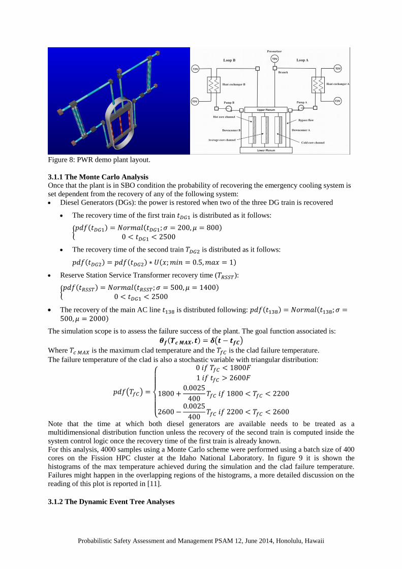
The case is a simplified PWR simulated by RELAP-7 during a Station Black Out condition. Figure 8
shows a visualization of the plant.
I/O interface
Probabilistic Safety Assessment and Management PSAM 12, June 2014, Honolulu, Hawaii
Figure 8: PWR demo plant layout.
3.1.1 The Monte Carlo Analysis
Once that the plant is in SBO condition the probability of recovering the emergency cooling system is
set dependent from the recovery of any of the following system:
Diesel Generators (DGs): the power is restored when two of the three DG train is recovered
The recovery time of the first train 𝑡𝐷𝐺1 is distributed as it follows:
{𝑝𝑑𝑓(𝑡𝐷𝐺1) = 𝑁𝑜𝑟𝑚𝑎𝑙(𝑡𝐷𝐺1; 𝜎 = 200, 𝜇 = 800)
0 < 𝑡𝐷𝐺1 < 2500
The recovery time of the second train 𝑇𝐷𝐺2 is distributed as it follows:
𝑝𝑑𝑓(𝑡𝐷𝐺2) = 𝑝𝑑𝑓(𝑡𝐷𝐺2) ∗ 𝑈(𝑥;𝑚𝑖𝑛 = 0.5,𝑚𝑎𝑥 = 1)
Reserve Station Service Transformer recovery time (𝑇𝑅𝑆𝑆𝑇):
{𝑝𝑑𝑓(𝑡𝑅𝑆𝑆𝑇) = 𝑁𝑜𝑟𝑚𝑎𝑙(𝑡𝑅𝑆𝑆𝑇; 𝜎 = 500, 𝜇 = 1400)
0 < 𝑡𝐷𝐺1 < 2500
The recovery of the main AC line 𝑡138 is distributed following: 𝑝𝑑𝑓(𝑡138) = 𝑁𝑜𝑟𝑚𝑎𝑙(𝑡138; 𝜎 =500, 𝜇 = 2000)
The simulation scope is to assess the failure success of the plant. The goal function associated is:
𝜽𝒇(𝑻𝒄 𝑴𝑨𝑿, 𝒕) = 𝜹(𝒕 − 𝒕𝒇𝑪)
Where 𝑇𝑐 𝑀𝐴𝑋 is the maximum clad temperature and the 𝑇𝑓𝐶 is the clad failure temperature.
The failure temperature of the clad is also a stochastic variable with triangular distribution:
𝑝𝑑𝑓(𝑇𝑓𝐶) =
{
0 𝑖𝑓 𝑇𝑓𝐶 < 1800𝐹
1 𝑖𝑓 𝑡𝑓𝐶 > 2600𝐹
1800 +0.0025
400𝑇𝑓𝐶 𝑖𝑓 1800 < 𝑇𝑓𝐶 < 2200
2600 −0.0025
400𝑇𝑓𝐶 𝑖𝑓 2200 < 𝑇𝑓𝐶 < 2600
Note that the time at which both diesel generators are available needs to be treated as a
multidimensional distribution function unless the recovery of the second train is computed inside the
system control logic once the recovery time of the first train is already known.
For this analysis, 4000 samples using a Monte Carlo scheme were performed using a batch size of 400
cores on the Fission HPC cluster at the Idaho National Laboratory. In figure 9 it is shown the
histograms of the max temperature achieved during the simulation and the clad failure temperature.
Failures might happen in the overlapping regions of the histograms, a more detailed discussion on the
reading of this plot is reported in [11].
3.1.2 The Dynamic Event Tree Analyses

Probabilistic Safety Assessment and Management PSAM 12, June 2014, Honolulu, Hawaii
The situation considered is exactly the one presented in the Monte Carlo analysis (3.1.2) and the
details of the analysis can be found in [11]. Figure 9 shows the time evolution of the clad temperature
and a projection of the sampling grid pattern generated by the dynamic event trees approach. The
green lines are the simulation continuing while the red dots signal a point where a simulation was
stopped since reaching the maximum clad temperature. It could be noticed that there are simulation
being stopped at a level of temperature that are exceeded by other simulations. The reason is of course
the random value of the clad failure temperature. On the left the plot shows a projection of the
threshold triggered by the Dynamic Event Tree simulation of the transient. The projection is
performed by defining the recovery time of the auxiliary system 𝒕𝑨𝑪 = 𝒎𝒊𝒏(𝒕𝑫𝑮𝟐, 𝒕𝟏𝟑𝟖, 𝒕𝑹𝑺𝑺𝑻). It is
clear how the competing variable (max clad temperature and AC recovery time) are alternatively
moved towards higher values of theirs CDF until a transition point between success failure is reached.
This pattern is generated by the contemporaneously sampling of two antagonist variables or in a
terminology more familiar in the RISMC framework by contemporaneously sampling the capacity and
the load. This aspect is discussed more in detail in [11].
Figure 9: On the left the max clad temperature for each of the branches generated by the dynamic
event tree. On the right the point sampled by the dynamic event tree.
3.1.3 Limit Surface Analysis
Figure 10, which is generated of the Monte Carlo Sampling in 3.1.1 shows clearly how (for a fixed
value of clad failure temperature) the limit surface is composed by three orthogonal planes. This is
clearly due to the fact that in essence the regions of possible system failure the max temperature in the
clad could be described by a linear relationship with the recovery time of the auxiliary system. The
success condition is therefore:
𝒕𝒇𝑪 > 𝒕𝑪 = 𝒕𝟎 + 𝜶 ⋅ 𝒎𝒊𝒏(𝒕𝑫𝑮𝟐, 𝒕𝟏𝟑𝟖, 𝒕𝑹𝑺𝑺𝑻)
In order to evaluate the limit surface search capability, that is still in a testing phase it was not used
directly the original case described in 3.1.1 but with the help of the API for the implementation of an
external model as described in 2.4 it was constructed a model returning:
𝒕𝑪 = 𝒕𝟎 + 𝜶 ⋅ 𝒎𝒊𝒏(𝒕𝑫𝑮𝟐, 𝒕𝑹𝑺𝑺𝑻) The model of course was not accurate in terms of numbers but it was supposed to show a similar
behavior even if one of the sampled recovery times was suppressed to allow a 3D visualization of the
limit surface for varying failure temperature of the clad.
Figure 10 shows the two limit surfaces obtained with a nearest neighbor (on the right) and radial basis
function (RBF) based surrogate models. Both limit surface show the two bounding planes compared to
the safe space (side of the surface with low recovery times) increase with the raising of the failure
temperature of the clad. This is clearly observable by the inclination of the planes. The nearest
neighbor as expected presents sharper edges with respect to the RBF kernel that instead tends to soften
the borders. The nearest neighbor algorithm closed the top of the surface erroneously; this unexpected
behavior is still under investigation.

Probabilistic Safety Assessment and Management PSAM 12, June 2014, Honolulu, Hawaii
Figure 10: Classification of the input space for the PWR SBO depending if during the simulation the
max clad temperature has been (failure, green), or have not been (success red) exceeded. To obtain a
3D plot the 𝑻𝒇𝑪 has been kept constant at 1477 K.
Figure 11: On the left the max clad temperature for each of the branches generated by the dynamic
4. CONCLUSION
RAVEN is reaching a level of maturity that might lead soon to a release of the code outside Idaho
National Laboratory to collect the first feedback. The statistical analysis framework based on grids and
Monte Carlo relies on very well assessed methodologies, and seems solid already. The integration of
those methodologies with the data handling flexibility, the visualization capabilities (all plots are
directly generated by the RAVEN code) and the ease of coupling with different physical model
simulators shows how RAVEN can be a powerful tool for PRA analysis. The dynamic event tree
implementation allows also a rapid turnaround time for the coupling with other codes as long as access
to the simulator of control logic is provided. The dynamic event trees has been identified as one of the
most promising approaches for PRA and at the same time it is foreseen its additional development to
introduce adaptivity.
Moreover the coming release of the code will the familiarize the PRA community with this enhanced
techniques like limit surface or surrogate model construction for identifying the leading mechanisms
of the system failure.
Acknowledgements
This work is supported by the U.S. Department of Energy, under DOE Idaho Operations Office
Contract DE-AC07-05ID14517. Accordingly, the U.S. Government retains a nonexclusive, royalty-
free license to publish or reproduce the published form of this contribution, or allow others to do so,
for U.S. Government purposes.
138 KV
Recovery
time
Diesel Generator
Recovery time
69
KV
Re
co
ve
ry T
ime

Probabilistic Safety Assessment and Management PSAM 12, June 2014, Honolulu, Hawaii
References
[1] D. Anders, R. Berry, D. Gaston, R. Martineau, J. Peterson, H. Zhang, H. Zhao, and L. Zou,
“Relap-7 level 2 milestone report: Demonstration of a steady state single phase pwr simulation
with relap-7,” Tech. Rep. INL/EXT-12-25924, Idaho National Laboratory (INL), 2012.
[2] C. Rabiti, A. Alfonsi, J. Cogliati, D. Mandelli, and R. Kinoshita, “Reactor analysis and virtual
control environment (raven) fy12 report,” Tech. Rep. INL/EXT-12-27351, Idaho National
Laboratory (INL), 2012.
[3] C. Rabiti, D. M. A. Alfonsi, J. Cogliati, and B. Kinoshita, “Mathematical framework for the
analysis of dynamic stochastic systems with the raven code,” in Proceedings of International
Conference of mathematics and Computational Methods Applied to Nuclear Science and
Engineering (M&C 2013), Sun Valley (Idaho), pp. 320–332, 2013.
[4] Alfonsi, C. Rabiti, D. Mandelli, J. Cogliati, and B. Kinoshita, “Raven as a tool for dynamic
probabilistic risk assessment: Software overview,” in Proceedings of International Conference
of mathematics and Computational Methods Applied to Nuclear Science and Engineering
(M&C 2013), Sun Valley (Idaho), pp. 1247–1261, 2013.
[5] Smith, C. Rabiti and R. Martineau, “Risk Informed Safety Margins Characterization (RISMC)
Pathway Technical Program Plan,” INL/EXT-11-22977, November 2012
[6] RELAP5-3D© Code Manual, Vol.1-5, Rev. 3, INEEL-EXT-98-00834 (2009)
[7] R.L. Williamson, J.D. Hales, S.R. Novascone, M.R. Tonks, D.R. Gaston, C.J. Permann, D.
Andrs, R.C. Martineau, “Multidimensional multiphysics simulation of nuclear fuel behavior”,
Journal of Nuclear Materials, 423 (2012) 149–163
[8] Boost Team, http://www.boost.org
[9] Christian Habermann, Fabian Kindermann, “Multidimensional Spline Interpolation: Theory and
Applications”, Computational Economics, Volume 30, Issue 2, pp 153-169, 2007
[10] William J. Gordon and James A. Wixom, “Shepard's Method of "Metric Interpolation" to
Bivariate and Multivariate Interpolation”, Mathematics and Computation, vol. 32, n 141, pp
253-264, 1978.
[11] Alfonsi, C. Rabiti, D. Mandelli, J. Cogliati, B. Kinoshita, and A. Naviglio. “Dynamic event tree
analysis through Raven”. In Proceedings of ANS PSA 2013 International Topical Meeting on
Probabilistic Safety Assessment and Analysis, Columbia (South Carolina), 2013.
[12] Gaston, G. Hansen, S. Kadioglu, D. A. Knoll, C. Newman, H. Park, C. Permann, and W.
Taitano, “Parallel multiphysics algorithms and software for computational nuclear engineering,”
Journal of Physics: Conference Series, vol. 180, no. 1, p. 012012, 2009.
[13] Pedregosa et al., “Scikit-learn: Machine Learning in Python”, Journal of Machine Learning
Research, pp. 2825-2830, 2011.

![[PPT]ALOHA FROM HAWAIIekladata.com/T87xXLe0Y72JoKgvTgg575PI2tM/Hawaiil.pps · Web view* HONOLULU - HARBOUR HONOLULU - AIRPORT HONOLULU IOLANI PALACE - HONOLULU ROYAL GUARD KAMEHAMEHA](https://static.fdocuments.in/doc/165x107/5af655b67f8b9a5b1e8effcd/pptaloha-from-view-honolulu-harbour-honolulu-airport-honolulu-iolani-palace.jpg)