- 1 -

Rattus Psychologicus: Construction of preferences by self-stimulating rats

Yannick-André Breton, James C. Marcus & Peter Shizgal

Concordia University, Montreal, Quebec, Canada

48 Pages, 6 Figures, 7 Tables

Corresponding Author: Peter Shizgal, 7141 Sherbrooke W., SP-244 Montreal, QC Canada H4B 1R6

- 2 -

Yannick-André Breton and Peter Shizgal are at the Groupe de recherche en neurobiologie

comportementale / Center for Studies in Behavioural Neurobiology (GRNC / CSBN),

Concordia University, Montréal, Québec, Canada. James C. Marcus is at the Department

of Psychology, Fordham University, Bronx, NY.

The authors thank Dr. Kent Conover for developing the curve-fitting procedure and

assisting the authors in its use.

This research was supported by grants from the Canadian Institutes of Health Research

and the Concordia University Research Chairs Program to Peter Shizgal as well as by a

grant from the “Fonds de la recherche en santé du Québec” to the GRNC / CSBN.

Correspondence concerning this article should be addressed to Peter Shizgal, Groupe de

recherche en neurobiologie comportementale/Center for Studies in Behavioural

Neurobiology, Concordia University, Room SP-244, 7141.Sherbrooke Street West,

Montreal, Quebec. H4B 1R6, Canada. E-mail: peter.shizgal@concordia.ca. Telephone:

+1-514-848-2424 ext 2191. Fax: +1-514-848-2817

- 3 -

Abstract

Behavioral economists have proposed that human preferences are constructed during

their elicitation and are thus influenced by the elicitation procedure. For example,

different preferences are expressed when options are encountered one at a time or

concurrently. This phenomenon has been attributed to differences in the “evaluability” of

a particular attribute when comparison to an option with a different value of this attribute

is or is not available. Research on the preferences of laboratory animals has often been

carried out by means of operant-conditioning methods. Formal treatments of operant

behavior relate preferences to variables such as the strength and cost of reward but do not

address the evaluability of these variables. Two experiments assessed the impact of

procedural factors likely to alter the evaluability of an opportunity cost (“price”): the

work time required for a rat to earn a train of rewarding electrical brain stimulation. The

results support the notion that comparison between recently encountered prices is

necessary to render the price variable highly evaluable. When price is held constant over

many trials and test sessions, the evaluability of this variable appears to decline.

Implications are discussed for the design of procedures for estimating subjective reward

strengths and costs in operant conditioning experiments aimed at characterizing,

identifying and understanding neural circuitry underlying evaluation and choice.

- 4 -

Introduction

In neoclassical economics, the individual economic agent is equipped with a

stable set of preferences that direct the maximization of self-interest. These preferences

are revealed by allocation decisions. Thus, an individual who has filled a shopping basket

with a particular set of goods is said to have revealed preferences that assign a higher

utility to the chosen “consumption bundle” than to any of the others that could have been

assembled at the same cost [41, 42].

Behavioral research has challenged the neoclassical view of the decision maker.

For example, preferences have been shown to depend on how options are described [49,

51] or on the method of elicitation [49]. As a result, normatively equivalent option sets

and methods of elicitation often give rise to systematically different responses [50]. Such

challenges have led to a new conception of human judgment in which preferences are not

merely revealed by the testing situation but instead constructed in the elicitation process.

As a consequence, preferences can be conceptualized as highly malleable and context-

dependent.

Among the illustrations of the malleability and context-sensitivity of preferences

are the anchoring effects of irrelevant, but highly accessible, information [1, 44] and the

reversals in preferences observed when objects encountered sequentially are presented

simultaneously [23]. Below, we illustrate these effects in human decision-making. Then,

we extend the notion of constructed preferences to choices made by non-human animals,

and we describe two experiments that demonstrate this phenomenon in laboratory rats

working for rewarding electrical brain stimulation.

- 5 -

An anchoring effect in humans. Simonsohn and Lowenstein [44] examined how much

money individuals spend on housing after moving between cities. Movers coming from

cities where housing was more expensive than in their new city viewed prices in the new

city as cheap and tended to spend more money initially on housing than individuals from

cities where housing was less expensive than in their new city. Thus, the irrelevant, yet,

readily accessible, information of prices in markets other than the local one served as

initial reference points in the construction of preferences for housing.

A preference reversal in humans. Hsee and colleagues [23] asked college students how

much they would pay for two CD changers. One of the CD changers was described as

having a capacity of 5 disks and a total harmonic distortion (THD: a measure of sound

quality) of 0.003% whereas the other changer was described as having a capacity of 20

disks and THD of 0.01%. Half of the participants were given no further information

about the THD measure whereas the others were told that the best and worst CD changers

on the market had THD values of 0.002% and 0.012%, respectively. Half of the

participants in each THD-information condition evaluated the two CD changers one at a

time whereas the others evaluated them jointly.

The experimenters surmised that disk capacity would be easy for the participants

to evaluate. In contrast, in the absence of information about the range of THD values in

the market, they expected that this measure would be difficult to evaluate and hence,

would have less influence over participants’ preferences than the capacity data. This is

what they found: participants who were not informed about the best and worst THD

values and evaluated the two CD changers one at a time were willing to pay more for the

- 6 -

one that scored higher on the easier to evaluate attribute (capacity); when the two CD

changers were evaluated jointly, the preference reversed, and participants were willing to

pay slightly more for the unit with the better sound quality. No such reversal was

observed in the participants who were told the THD values for the best and worst CD

changers on the market. Thus, the procedure for eliciting the preferences influenced the

results, but only when there was a large difference in the evaluability of the two

attributes.

Preference measurement in non-human animals. Theoretical treatments of the

preferences of non-human animals share several common assumptions with the

neoclassical approach to economics. The agent is often assumed to be maximizing some

proxy for fitness [29, 37, 38, 47, 48, 52], and its preferences are often assumed to be

revealed by behavioral-allocation decisions [7, 18, 31].

Experimental studies of judgment and decision in non-human animals often

employ operant-conditioning methods. A particularly convenient method for carrying out

such studies is to reward operant performance by delivering electrical stimulation to

appropriate brain regions [34]. No satiation is induced by “consumption” of the reward

[33], and experimental subjects are willing to work vigorously for this reward throughout

long test sessions [20]. The behavior of these subjects is exquisitely sensitive to variables

such as the strength [3, 46], rate [14, 36], and delay [15, 28] of reward.

In a typical operant-conditioning study carried out using electrical stimulation as

the reward, the value of an independent variable, such as the strength or cost of the

reward, is varied over a set of test trials [10, 30]. For example, the first trial in the series

- 7 -

is often carried out using the strongest reward available, and then the strength of the

stimulation is decreased in step-wise fashion (“swept”) from trial to trial until the subject

ceases to respond. This is the “curve-shift” procedure for measuring the reward-

modulating effects of drugs, lesions, and manipulation of physiological need states: the

effectiveness of the reward-modulating manipulation is estimated from lateral

displacement of the curve relating the vigor (e.g., the rate) of performance to the strength

(e.g., the pulse frequency) of the electrical stimulation [10, 30]. In these studies, changes

in the reward effectiveness of brain stimulation are inferred from changes in the

stimulation strength that produces a criterion level of performance, such as the half-

maximal level (the “M50”). Alternatively, the cost of the stimulation (e.g., the number of

times the subject must respond to earn a reward) can be varied in lieu of its strength, as in

the “progressive-ratio” method [24]. The position of the psychometric function along the

cost axis is taken as index of the subject’s willingness to pay for the reward.

In the literature on application of curve-shift methods, the position of the

psychometric function on the axis representing the independent variable (e.g., stimulation

strength or cost) is generally taken as an index of an internal determinant of decision,

such as reward effectiveness [3, 30] or willingness to invest effort in the pursuit of reward

[32, 39, 40]. The performance of the subject can be construed as a reflection of an

underlying preference between the payoff derived from “work,” defined as operant

performance for reward and that derived from “leisure,” defined as alternative activities

such as grooming, exploring, and resting [4, 7, 9, 21]. Such preferences are thought to be

revealed by the scaling procedure. Although several studies have examined whether

behavioral allocation depends on the direction (ascending or descending) in which the

- 8 -

value of an independent variable is swept [13, 25, 26, 35], we know of no prior work

assessing the possibility that the preferences for rewarding brain stimulation are

constructed in a manner akin to those manifested by human subjects.

If the preferences of non-humans animals between work and leisure are

constructed rather than revealed, then they may well be subject to anchoring effects and

preference reversals akin to those demonstrated in human subjects; such preferences

would depend on the procedure used to elicit them. We investigated these issues in

laboratory rats working for brain stimulation reward (BSR). Psychometric functions

relating the allocation of behavior to the strength of the stimulation (the pulse frequency)

were obtained as described above. Cost was defined and manipulated in terms of the

work time required to earn a reward (an “opportunity cost”). This work requirement—

hereafter termed the “price”—remained constant throughout a series of repeated

frequency sweeps. Thus, a rat working for rewards at a price of four seconds was

required to hold down a lever (on average or exactly, depending on the schedule of

reinforcement) for four seconds per reward. Once a set of frequency sweeps had been

collected at a low price, the price was increased to a medium value, and a new set of

frequency sweeps was run. Then, the price was further increased to a high value, and

another set of frequency sweeps was obtained. The procedure was then reversed by

decreasing the price, in a step-wise manner, from high to medium to low, and running a

set of frequency sweeps at each price. At the end of this series of rising and falling prices,

price sweeps were run: with the stimulation frequency held constant at a high value, the

price was increased systematically from trial to trial. In a second experiment, the subjects

were exposed to the same set of pulse frequencies and prices, but instead of sweeping the

- 9 -

value of one independent variable across trials with the other independent variable held

constant for many sessions, both the pulse frequency and the price were sampled

randomly, and multiple values of both variables were encountered in each test session.

If performance is determined solely by the strength and cost of the reward, then

the order of presentation should not matter, and the results obtained with random

sampling of parameter values should be equivalent to those obtained by systematically

sweeping the strength and cost variables. Such preferences would be said to be

“procedurally invariant.” In contrast, if the preferences of the rats are constructed in the

course of testing, they should depend on factors in addition to the strength and cost of the

currently available reward, which may include the anchors provided by preceding testing

conditions and the evaluability of the independent variables. If so, different results should

be obtained when parameter values are sampled randomly or systematically.

Revealed-preference predictions. Figure 1 demonstrates how the effect of systematically

increasing and decreasing the price of BSR alters the allocation-frequency relationship in

a hypothetical subject that is insensitive to anchoring effects and can evaluate both the

strength and price of the stimulation with equal ease. In panel A, the proportion of time

allocated to the operant task is plotted as a function of pulse frequency. As the pulse

frequency is decreased, time allocation decreases from maximum to minimum. An

increase in price must be offset by a compensatory increase in reward strength and hence,

in pulse frequency. Thus, the dashed curve (medium price) lies to the right of the solid

curve (low price). An additional rightward shift is produced by increasing the price from

a medium value to a high one (dotted curve). However, this last displacement is

- 10 -

accompanied by a decrease in maximal time allocation. The reason for this prediction is

that the rewarding effect is known to saturate at high pulse frequencies [43]. Once the

frequency approaches the reward-saturating value, further increases no longer suffice to

offset increases in price, and pursuit of the rewarding stimulation can no longer dominate

competing activities, such as grooming, resting, and exploring.

Panel B plots the pulse frequencies (“M50” values) at which each of the curves in

Panel A attains a half-maximal level of time allocation. Since the subject is presumed to

be insensitive to anchoring effects, the same M50 values are obtained for both of the

curves obtained at the low (squares) and middle (circles) prices, regardless of whether

these prices are tested during the ascending (solid symbols) or descending (open

symbols) price series.

In Panel C, the curve produced by sweeping the price at one pulse frequency is

shown along with the curve obtained by sweeping the pulse frequency at the highest

price. In a subject whose preferences are procedurally invariant, the curves obtained from

the price sweep should be consistent with those obtained from the frequency sweep.

Regardless of whether a particular combination of pulse frequency and price is

approached along a frequency-sweep, or price-sweep curve, the same time allocation

should be obtained. The single time allocation at the point in the parameter space (the

floor of the graph) where the two sweeps intersect is denoted by a sphere.

Predicted effect of anchoring. Panel D of Figure 1 plots the proportion of time allocated

to self-stimulation as a function of pulse frequency in a hypothetical subject whose

preferences are susceptible to the anchoring effects of previous reinforcement history. By

- 11 -

analogy to the literature on human construction of preference [44], low prices appear

lower when an individual’s scale of evaluation has been anchored at a higher price, and

high prices appear higher when an individual’s scale of evaluation has been anchored at a

lower price. As a result, one would expect subjects whose evaluation of the current price

is anchored by previously encountered prices to have lower M50 values when the previous

price condition was higher than the current condition, and higher M50 values when the

previous price condition was lower than the current condition. Panel E plots the M50

values obtained from each price condition in such a subject.

Panel F illustrates the prediction that a subject manifesting anchoring effects will

show inconsistent time allocation when a given point in the parameter space is

approached along a price sweep or a frequency sweep. The frequency-sweep curve has

been pushed rightward due to anchoring, as shown in Panels D and E, thus reducing time

allocation at the point in the parameter space where the two curves cross. Given that a

range of rapidly changing prices is encountered repeatedly during price-sweep tests, an

anchoring effect is not anticipated. Thus, time allocation is predicted to be higher during

when the cross point is approached along a price sweep than along a frequency sweep.

Predicted effect of reduced evaluability. During the first experiment, the price of the

stimulation was held constant over many sessions while the strength of the stimulation

was varied. The absence of comparison prices during each testing session may have

reduced the evaluability of the opportunity cost. If so, the effect of the price on

behavioral allocation would be expected to be greater during the second experiment,

when both the strength and the cost of the stimulation varied over the course of each

testing session.

- 12 -

If, in the first experiment, the opportunity cost were far less evaluable than

stimulation strength, one would expect the rat to rely primarily on the strength of the

reward rather than its price to allocate behavior between work and leisure activities. This

insensitivity to price, in its most extreme case, would result in zero displacement of the

frequency sweep curves. A rat incapable of accurately evaluating the opportunity cost of

BSR would not require any compensatory increase in stimulation frequency following a

price increase. Panels G and H of Figure 1 illustrate a slightly less extreme hypothetical

case, in which the evaluability of the price variable is very low, but not zero. The lower

the evaluability of the price variable, the closer a plot of the M50 values across the

different phases of the experiment to a vertical line.

Panel I illustrates the prediction that a subject sensitive to the evaluability of the

price variable will show inconsistent time allocation when a given point in the parameter

space is approached along a price sweep or a frequency sweep; the inconsistency in

allocation should be opposite to that manifested by a rat that is subject to anchoring

effects. Due to the poor evaluability of the price variable during frequency-sweep testing,

the frequency-sweep curve obtained at the highest price will be little displaced from the

ones obtained at the low and middle prices, as shown in Panels G and H. However, the

repeated encounters with multiple prices during price-sweep testing renders the price

more evaluable and restores the effectiveness of this variable, thus lowering time

allocation at the cross-point.

The present experiments demonstrate that the preferences of rats working for BSR

differ from the procedurally invariant ones depicted in Panels A-C of Figure 1.

- 13 -

Systematic anchoring effects (Panels D-F) were not evident. However, the influence of

price was greater when multiple prices were encountered during each test session and

hence, the evaluability of this variable was high, than when the price was held constant

over many test sessions and hence, the evaluability of this variable was low (Panels G.H).

Moreover, performance at the cross-point between the high-price frequency sweep and

the price sweep was greater when this point in the parameter space was approached along

a frequency sweep than along a price sweep, as one would expect if the evaluability of

the price variable were low during frequency-sweep testing (Panel I). This violation of

procedural invariance was eliminated by random sampling of frequencies and prices,

which also boosted the influence of the price variable.

Experiment 1

Materials and Methods

Subjects were seven experimentally-naïve, male Long-Evans rats (Charles River,

St-Constant, Quebec) weighing at least 450 grams at the time of surgery. Under sodium

pentobarbital anesthesia, monopolar stimulation electrodes insulated to within 0.5 mm of

the tip were aimed stereotaxically at the lateral hypothalamic level of the medial

forebrain bundle, either unilaterally or bilaterally. Coordinates were 2.8 mm posterior to

bregma, 1.7 mm lateral to the midline and 9mm from the skull surface.

Throughout the experiment, stimulation consisted of 0.5 s trains of monophasic,

cathodal, constant-current pulses, 0.1 ms in duration. Following at least four days of

- 14 -

recovery from surgery, the subjects were shaped to press a lever that triggered a

stimulation train. The criterion for inclusion in the study was avid responding for 78 Hz

trains of 200 µA pulses in the absence of involuntary stimulation-induced movements or

evident signs of aversion such as vocalizations, withdrawal from the lever, or escape

behaviors. Further testing was carried out to determine the highest current at which a

wide range of pulse frequencies supported lever pressing in the absence of disruptive side

effects, such as escape behaviors and forced movements. The currents selected for rats

CP2, CP3, CP7, CP8, CP9 and C26 were, respectively, 700, 500, 600, 300, 700 and 1260

µA.

Following screening, the rats were trained to hold down a lever in order to trigger

the rewarding stimulation. A zero-hold, variable interval schedule [7] was in effect. On

this schedule, the rat was rewarded only if the lever was held down at the end of an

interval randomly sampled from an exponential distribution. The parameter of this

distribution was the average time the lever had to be depressed (“work time”) to obtain a

reward. By analogy to concept of opportunity cost in economics, this work time is called

the “price” of the reward. The average price during training was set to 1 s.

A cue light over the lever was illuminated whenever the lever was depressed. If

the lever was not depressed at the end of the current interval, a new interval was selected

and the timer restarted. As soon as a reward was triggered, the lever was retracted, and

the interval timer was paused. After a 2-s delay, the lever was re-introduced into the cage,

and the timing of a new interval began.

- 15 -

A trial consisted of a period of time during which both the average price and the

strength of the rewarding stimulation were held constant. In both experiments, the trial

time was set at 20 times the average price, thus allowing the rat to harvest 20 rewards per

trial if working continually. An orange house light flashed throughout the ten-second

interval separating one trial from the next. Levers were retracted and cue lights turned off

for the duration of this inter-trial interval.

Once the rats had acquired the operant response, daily sessions were carried out,

consisting of 12 determinations of a 10-trial sequence in which the pulse frequency was

decreased in equal logarithmic steps from trials 2 through 10, over a range that drove the

proportion of time the lever was depressed (“time allocation”) from maximal to minimal.

Trial 1 served as a warm-up, and the pulse frequency was the same as on trial 2. The

tested frequency ranges for rats CP2, CP3, CP7, CP8, CP9 and C26 were 334-100, 166-

24, 182-50, 114-62, 200-50 and 170-58 Hz, respectively. The steps sizes used in this first

phase were 0.065, 0.10, 0.07, 0.03, 0.07 and 0.06 common logarithmic units,

respectively.

Following training on the frequency sweep procedure, animals were trained on the

price sweep procedure. The pulse frequency was set at a high value while the average

price on each trial was increased in equal logarithmic units, driving performance from

maximum to minimum. As in the frequency-sweep procedure, the first trial of each

determination served as a warm-up, followed by nine trials over which the price was

increased. The zero-hold variable-interval schedule of reinforcement was still in effect.

The large amount of time required to collect data from each determination precluded

exclusion of the first determination from the analysis. The tested price range was 1-30.2s;

- 16 -

the step size used in this second, price-sweep phase was therefore 0.185 common

logarithmic units.

Psychometric curves were plotted, relating time allocation to the common

logarithm of the pulse frequency. Once at least 20 determinations were obtained over

which the position of the psychometric curves along the logarithmic pulse-frequency axis

did not vary by more than 5% within sessions and 10% between sessions (as determined

by visual inspection), the price of the sweeps was increased to the geometric mean of 1s

(the price of the rewards during the initial frequency sweep) and the price that produced

50% time allocation during price-sweep training. Another set of 20 or more

determinations were run at this higher, “medium” price. A final set of 20 stable

determinations was obtained at the “high” price that had produced 50% time allocation

during the price-sweep training. The low price was always 1 s; the medium and high

prices for each rat are shown in Table 1.

Following three sets of frequency-sweeps at escalating prices, the sequence of

price changes was repeated in reverse order. The price of the reward was decreased back

to the medium value for 20 or more frequency-sweep determinations, and again to the

low price for 20 or more determinations. At the conclusion of this first experiment, a final

series of price-sweeps was obtained at a high frequency. Thus, a total of five or six

sweeps types were run with each rat. In order, these were: a first low-priced frequency

sweep, a first medium-priced frequency sweep, a high-priced frequency sweep, a second

medium-priced frequency sweep a second low-priced frequency sweep and a high-

- 17 -

frequency price sweep. The second low-priced frequency sweep was omitted in the cases

of rats C26, CP2 and CP3.

The first determination in each test session was considered a warm-up, and the

data were excluded from the analysis; the data from the first session of each phase were

also excluded.

A separate group of 5 rats was tested to assess the baseline variability in the

frequency-sweep data over the course of long-term testing. Rats DE1, DE2, DE3, DE4

and DE7 underwent the same surgical and training procedures as the rats in the

experimental group. As in the experimental group, the schedule of reinforcement ensured

that the number of rewards obtained was proportional to the time that the lever was

depressed. However, the work time required to obtain a reward was fixed at a constant

price of 1 s. The number of test sessions for these “drift-control” subjects equaled the

median for the experimental subjects, and the number of determinations per session

matched the median number for the corresponding session performed with the

experimental subjects. Thus, the drift-control subjects underwent a first phase of testing

that consisted of 3 13-determination sessions (thus matching the first pass though the

low-price condition for the experimental group), a second phase consisting of another 3

13-determination sessions (matching the first pass through the medium price condition

for the experimental group), a third phase consisting of 7 5-determination sessions

(matching the high-price condition for the experimental group), a fourth phase consisting

of 3 13-determination sessions (matching the second pass through the medium price

condition for the experimental group) and a fifth phase consisting of a final 3 13-

- 18 -

determination sessions (matching the second pass through the low-price condition for the

experimental group).

The first determination in each test session was considered a warm-up, and the

data were excluded from the analysis; the data from the first session of each phase were

also excluded. (An exception was made in the case of rat DE2 due to data loss resulting

from a broken lead; data from session 1 in phases 2 and 5 were retained to replace the

incomplete session 3 in phase 2 and session 2 in phase 5.) Thus, the analysis of the drift-

control data was based on 24 frequency-sweep determinations in each of the five phases,

all carried out at a 1-second price.

- 19 -

Results

The dependent variable

The dependent measure in the data analyses was a corrected estimate of time

allocation [6, 7]. The raw measure of time allocation was the ratio of work time (time

spent holding down the lever) to trial time (the total time the lever was extended and

reward was available). The denominator of the time-allocation ratio can also be expressed

as the sum of the work time, as defined above, and the “leisure time,” during which the

rat performed alternate activities such as grooming and exploring. Leisure time is

estimated from the sum of the intervals during which lever is not depressed [7]. Conover

has determined that when the strength of the stimulation is high and the cost is low,

individual leisure bouts comprise at least two populations, one consisting of intervals

sufficiently long to perform alternate activities and another consisting of very short

intervals (< 1 s) [5]. During the brief latter pauses in responding, the rat remains near the

lever, often with its paw resting lightly upon it. Thus, these brief pauses appear to be part

of the behavior pattern associated with work rather than with leisure activities. For this

reason, pauses shorter than 1 s in duration were subtracted from the leisure time and

added to the work time so as to arrive at the corrected estimates of time allocation that

were used in the analysis of the data.

Curve-fitting procedure

Dual-quadratic functions were fit to the data collected in each sweep condition by

means of a bootstrapped [12], least-square procedure. These functions were defined

piecewise as horizontal upper and lower segments joined by two separate quadratic

- 20 -

functions. Smooth junctions between segments were ensured by requiring that the first-

order derivatives be equal on each side of the intersection between a given segment and

its neighbor. A dual-quadratic spline function was used in lieu of broken-line [16] or

logistic [8] functions, because it is capable of describing quasi-sigmoidal datasets that are

asymmetric about their midpoints.

The bootstrapped curve-fitting procedure was implemented using MATLAB (The

Mathworks, R2007b). By sampling with replacement from the data obtained at each point

along a sweep, 1000 re-sampled datasets were generated; the number of observations at

each point along a sweep was equal to the number of determinations that had been run.

For example, if 20 determinations of a frequency sweep had been run, then the

bootstrapping procedure generated 1000 frequency-sweep datasets consisting of 20

observations at each pulse frequency. A dual-quadratic spline function was fit to each of

the 1000 curves obtained by resampling the data from a given price condition. This

yielded 1000 estimates of the frequency that produced half-maximal time allocation and

of the average time allocation for each pair of pulse frequency and price values for both

frequency and price sweeps. The estimated frequency that produced half-maximal time

allocation is analogous to the M50 measure of Miliaressis et al. [30]. The 95% confidence

interval around each estimate was defined as the region excluding the lowest 25 and

highest 25 of the 1000 estimates.

Frequency-sweep data

Figures 2a and 2b show the curves fitted to the frequency-sweep data along with

the mean time allocation for each frequency and the associated 95% confidence intervals.

- 21 -

The inset shows the mean frequency corresponding to half-maximal time allocation (M50)

for each curve over the ascending and descending series of prices. In the inset, dotted

lines join the M50 values for corresponding prices in the ascending and descending series.

The degree to which these dotted lines deviate from the vertical indicates the level of

inconsistency between the estimates obtained in the ascending and descending series of

prices.

In the cases of four of the seven subjects, the M50 profiles correspond roughly to

the expected triangular form, and in the case of another subject, a triangular profile is

seen over the three central conditions (middle1, high, middle2). Even in these cases, the

vertical dotted lines joining corresponding prices deviate from the vertical.

The shifts in M50 values corresponding to each price change are shown in Table 2.

Each value in this table represents the difference between the estimates obtained at a

given price and the estimate obtained at the next price tested. The statistical criterion for a

reliable shift was an absence of overlap between the 95% confidence intervals

surrounding the two estimates from which the shift is derived (denoted by asterisks).

Table 3 shows the differences between the M50 values obtained at the low and

middle prices in the ascending and descending price series. Asterisks denote cases in

which the 95% confidence intervals surrounding each of the M50 estimates do not

overlap. Deviations of the dotted lines from the vertical in the lower insets of Figures 2A

and 2B are proportional to the values in this table. These deviations show the degree to

which inconsistent M50 values were obtained in the ascending and descending price

series.

- 22 -

The data from the “drift-control” subjects, which are shown in Figure 3, provide

an estimate of baseline variability in M50 measures. All five sets of curves were obtained

at the same price. Thus, if performance were perfectly stable over time, the profile of the

M50 measures would be vertical. Note that some of the profiles deviate substantially from

a vertical line, and that the magnitude of the inconsistencies between the M50 values for

the different curves overlaps that observed in the data from the experimental group.

Tables 4, and 5 show the shifts in M50 values observed in the data from the drift-

control subjects. The shifts were calculated between data sets matched to those in which a

given price was tested in the experimental group. For example, the middle price was in

effect in the second and fourth frequency-sweeps obtained from the experimental

subjects. Thus, the corresponding shifts in the drift-control data were between the values

obtained in the second and fourth data sets. Similarly, the shifts between the first and fifth

data sets in the drift-control data correspond to the shifts between the two low-price

frequency sweeps in the experimental group.

The relative effect of price changes on the M50 values for the subjects in the

experimental and drift-control groups was assessed by means of a non-parametric test

(Mann-Whitney U). The changes in M50 values were expected to be larger in the subjects

that experienced price changes (those in the experimental group) than in the subjects that

were tested with a constant price (the drift-control group). Thus, single-tailed tests were

performed. The results are reported in Table 6. All the comparisons exceed the statistical

threshold. Thus, despite the substantial variation across subjects, the price variable did

- 23 -

produce a detectable effect, even when the drift in M50 values across sessions is taken

into account.

Non-parametric tests were also carried out to determine whether the inconsistency

between M50 values from the ascending and descending prices in the experimental group

exceeded the discrepancies that arose in the drift-control group during repeated testing

under constant conditions. One test was carried out on the signed differences between the

shifts observed between corresponding data sets from the two groups, and a second test

was carried out on the absolute value of the shifts. In neither case did the result meet the

criterion for statistical significance (U=9 and U=14 signed, U=7 and U=16 unsigned, p

>0.05, two tailed). Thus, the inconsistency observed between M50 values for curves

obtained a given price in ascending or descending price series in the experimental group

was not greater than what would be expected on the basis of the variability observed in

the control group.

Comparison of frequency- and price-sweep data

The left side of Figure 4, shows the 95% confidence intervals surrounding the

curves fitted to the high-priced frequency sweep data (black) and those fitted to the price

sweep data (grey) for a single rat. The vertical dashed line indicates where the two curves

cross in the parameter space (the floor of the three-dimensional graph). The rat’s time

allocation to lever pressing at the intersection point, as determined by the fitted curve, as

well as the 95% confidence region surrounding the estimate for frequency sweep data

(black) and price sweep data (grey), are depicted in the upper left panel of the array of

graphs on the right side of Figure 4. If the rat’s preferences were procedurally invariant,

- 24 -

these two time-allocation values should be same. Clearly, they are not, as is indicated by

the large distance between the two means and the non-overlap of the associated 95%

confidence intervals. The remaining panels in the array on the right side of Figure 4

provide analogous estimates for all the rats. In all 7 cases, the time allocation estimated

by the curve fit to frequency sweep data is significantly greater than that fit to the price

sweep data (p<0.05, bootstrapped). Thus, the procedure used to derive the psychometric

curves (frequency sweeps versus price sweeps) influenced the time-allocation estimates,

and procedural invariance was violated.

Discussion

Three predictions arise from the hypothesis that the preferences of self-

stimulating rats are revealed by their reward-seeking behavior and do not depend on the

procedures used to elicit them: (1) M50 values for frequency sweeps should increase as

the price is raised and decline as the price is lowered; (2) M50 values for frequency

sweeps obtained at a given price should be the same, regardless of whether they pertain to

sweeps run during the ascending-price or descending-price phase of the experiment; (3)

time allocated to working for BSR at a particular price and frequency should be the same,

regardless of whether that pair of price and frequency values is embedded in a frequency

sweep or in a price sweep.

Prediction 1: changes in M50 values as a function of price

The payoff from a train of rewarding stimulation depends both on its strength and

its price [17, 27]. Thus, in order to hold time allocation constant following an increase in

price, a compensatory increase in pulse frequency should be required. If preferences

- 25 -

between work and leisure depend only on the strength and price of the reward, and

preferences are simply revealed by the testing procedure, then M50 values should increase

systematically during the ascending-price phase and decrease systematically during the

descending-price phase. As a result, a subject whose preferences depend only on the

strength and price of the reward will require higher frequencies to achieve an equivalent

level of performance when the price is increased to a medium or high value: curves

relating time-allocation to the common logarithm of the pulse frequency (“allocation-

frequency curves”) obtained at medium and high prices will be shifted rightward with

respect to those obtained at low and medium prices, respectively. Similarly, allocation-

frequency curves obtained at lower prices will be shifted leftwards with respect to those

obtained at higher prices.

Table 2 provides evidence that systematic changes in M50 values were indeed

observed in most subjects. In the results from rats CP7, CP8, and CP9, all four shifts in

M50 values (low 1 to medium 1, medium 1 to high, high to medium 2, medium 2 to low

2) surpass the statistical criterion. This is also the case for three of the four shifts

observed in the data from rat CP4 and in two shifts (medium1 to high, high to medium 2)

for rat C26. Overall, the magnitude of the changes in M50 values obtained in the subjects

exposed to price changes (the experimental group) was larger than in the subjects tested

repeatedly at a constant price (the drift-control group).

These results provide only modest support for the prediction of systematic shifts

in M50 values. Two subjects failed to show the expected pattern of shifts, and many of the

shifts in the remaining subjects were rather small in comparison to the price changes. For

example, the shifts obtained in rat CP7 in the medium 1 to high and high to medium 2

- 26 -

conditions were only 0.026 and -0.024 common logarithmic units. In this rat, the medium

and high prices were 4 and 16 s, respectively, values spaced 0.60 common logarithmic

units apart. The growth of the subjective intensity of the rewarding effect as a function of

the pulse frequency would have to have been unprecedented in steepness in order for

such small changes in pulse frequency to offset such large changes in price. Gallistel and

Leon [18] reported that reward intensity grows roughly as a power function (with an

exponent varying from approximately 2 to 10) over modest frequency intervals.

Assuming that reward value is determined by the ratio of subjective reward intensity to

subjective price [7] and that subjective price closely mirrors objective price over the

range from 4-16 s [45], the exponent of such a power function would have to be in the

range of 23 - 25 in order for the small frequency shifts observed in rat CP7 to compensate

for the fourfold ratio of middle and high prices.

A more likely account of the data is that the evaluability of the price variable was

low in this experiment due to the fact that each set of the 20 or more frequency sweeps in

each condition were carried out at a constant price. In order for the price variable to be

fully evaluable, it may be necessary for the rat to encounter two of more different price

values in the same test session. This hypothesis is tested in Experiment 2.

Prediction 2: consistency of M50 values across the ascending- and decreasing-

price series

In five of the seven rats, statistically reliable differences were found between M50

values for a given price in the ascending and descending price series (Table 2). However,

the direction of these shifts varied across subjects, and their magnitude was not

significantly different from the magnitude of the shifts observed in the drift-control group

- 27 -

over the course of repeated testing at a constant price. Thus, there is no firm evidence that

the preceding price condition served as an anchor for evaluating the price currently in

effect. Of course, if the evaluability of the price variable were low in this experiment, any

anchoring effect would have been minimized.

Prediction 3: consistency of price- and frequency-sweeps

If the preferences of the rats were procedurally invariant, time allocation to any

single combination of prices and pulse frequencies should not have depended on whether

a particular location in the parameter space (a pair of price and frequency values) is

visited in the course of a frequency sweep or a price sweep. This was not the case. In all

seven rats, time allocation was higher at the intersection of the vectors composed of the

tested frequencies and prices when this point was approached during a high-price

frequency sweep than during a price sweep. Thus, procedural invariance was violated in a

consistent manner. The direction of the violation is consistent with the notion that the

evaluability of the price variable was lower during frequency sweeps, when the price was

constant, than during price sweeps, when the price varied from trial to trial.

Due to an oversight, the schedule of reinforcement in effect for the drift control

animals differed from that in effect for the experimental animals. Given that the price was

constant within trials for the drift-control subjects but variable for the experimental

subjects, the data from the former group would be expected to be more stable than those

from the latter group. Thus, by reducing noise in the control group, this procedural

difference should have made it easier to discern an anchoring effect. The failure to

observe such an effect is thus all the more striking. That an anchoring effect was not seen

- 28 -

could well have been due to decreased evaluability of the price variable in the frequency-

sweep conditions.

- 29 -

Experiment 2

Two of the findings of Experiment 1 are consistent with the idea that the

evaluability of the price variable was low during prolonged frequency-sweep testing at a

constant price. First, the changes in pulse frequency required to offset price changes were

smaller and less consistent than expected, as though the influence of the price variable

had been weakened. Second, more time was allocated to working for stimulation trains at

a particular frequency and price when that point in the parameter space was encountered

in the course of the high-price frequency sweep than in the course of the price sweep.

Thus, the ability of higher prices to attenuate performance appeared greater when a

comparison price was available during the same testing session.

In Experiment 2, multiple frequencies and prices were encountered during each

test session. It was expected that this would increase the evaluability of the price variable.

Consequently, more robust and consistent shifts were anticipated in the frequencies

required to sustain a given level of time allocation as a function of price changes.

To maintain the evaluability of the pulse frequency, fixed comparison frequencies

were presented immediately prior to and following each experimental trial. The lead

comparison frequency produced a near-maximal reward whereas the trailing comparison

frequency produced a minimal reward. Thus, the comparison frequencies defined the

available range of subjective reward intensities.

The prices and frequencies tested were the same as in Experiment 1, but the

values of the two variables were no longer swept sequentially and were presented instead

in random order. The vectors composed of the frequencies tested at the high price and the

- 30 -

prices tested at the highest frequency intersected at the same point in the parameter space

as in Experiment 1. However, it was expected that due to the increased evaluability of the

price variable and the use of a common procedure to sample the points along the

frequency and pulse vectors, consistent time allocation would be observed at the

intersection.

Materials and Methods

Five of the rats tested in Experiment 1, rats C26, CP4, CP7, CP8 and CP9, served

as subjects. The 36 price-frequency pairs tested were the same as in Experiment 1, as

were the currents, pulse waveform, pulse duration, and train duration.

The pulse frequencies and prices were placed in a list. Given that variability of

time allocation is highest on the steeply rising portion of the psychometric curve, points

in this region were tested more frequently than those at the upper and lower extremes of

the curves. Thus, the central three points of each frequency or price vector were

represented twice in the list, and the remaining points were represented once. The list was

then randomized. A new list of pseudo-randomized test points was generated every day

using custom-programmed software in the MATLAB programming language.

Test sessions consisted of a series of experimental trials bracketed by trials on

which the comparison frequencies were presented. On the leading comparison-frequency

trial, the pulse frequency was as high as the rat could tolerate whereas on the trailing

comparison-frequency trial the pulse frequency was too low to support lever pressing

(10Hz). The price was set to 1 s on both comparison-frequency trials. The experimental

- 31 -

trials were drawn from the randomized list without replacement until all test trials had

been presented once (for the extremes) or twice (for the middle points) during a single

test session. The maximum session duration was 6 hours.

A fixed, “cumulative handling-time” schedule was in effect. On this schedule,

every reward in a given trial was delivered after the cumulative time the lever had been

depressed equaled the price specified in question in the randomized parameter list. As in

the case of the zero-hold variable-interval schedule used in Experiment 1, the number of

rewards earned was proportional to the time allocated to work (holding down the lever).

However, the fact that the work time required to obtain a reward was fixed within a trial

minimized the time required for the rat to adjust to each new price. In principle, the rat

could determine the price in effect on each trial after earning a single reward. In contrast,

on the zero-hold variable-interval schedule, the price for each reward is drawn randomly

from an exponential distribution. Thus, the rat must encounter many rewards under the

zero-hold variable-interval schedule in order to obtain a good estimate of the parameter

of the price distribution. (For example, 352 rewards must be encountered in order for the

95% confidence interval surrounding the average price encountered to fall within 10% of

the set price.) This did not pose a problem in Experiment 1. For example, identical

frequency sweeps were run at least 21 times in a row at a given price. Thus, there was

ample opportunity to estimate the mean of the exponential distribution of prices.

However, in Experiment 2, prices were determined from randomized lists, and the rat had

to estimate the price anew on each and every experimental trial. Thus, it was necessary to

hold the price constant within each trial in order to minimize the time required for price

estimation.

- 32 -

Results

Given that pulse frequencies and prices were selected from randomized lists, the

rat could not know at the start of an experimental trial what price would have to be paid

to obtain the pulse train or at what frequency the pulses would be delivered. Only on

delivery of the first reward, were these quantities revealed. Therefore, time elapsed prior

to the delivery of the first reward was eliminated from the calculation of time allocation.

Otherwise, time allocation was calculated as in Experiment 1.

The data were grouped into four matrices corresponding, respectively, to the low-

price frequency sweeps, middle-price frequency sweeps, high-price frequency sweep, and

price sweep from Experiment 1. Separate columns of each matrix stored the pulse

frequency, price, and time allocation. The matrices were sorted to yield the same

sequences of pulse frequencies or prices that were swept in Experiment 1. For example,

once sorted, the matrix corresponding to the low-price frequency sweep from Experiment

1 contained the same series of pulse frequencies as was employed in that experiment, and

the price column contained a constant value: the low price. Psychometric curves were

obtained by fitting dual-quadratic functions to the time-allocation data in the matrices,

using the same bootstrap-based procedures employed in Experiment 1, and M50 values

were derived.

The fitted psychometric curves are shown in Figure 5 Increases in price shift these

curves rightwards (Table 7). The insets compare the M50 values obtained from

Experiments 1 and 2. Note that in all cases, the trajectory described by the M50 values as

- 33 -

price is increased lies further from the vertical in the case of Experiment 2 (heavier black

lines) than Experiment 1 (finer grey lines), indicating that the influence of the price

variable was greater. Further evidence of the augmented influence of the price variable

can be seen in the dramatic decline of time-allocation values at the highest price tested

(green points and curve in Figure 5). (In the case of rat CP4, time allocation is so

diminished that the curve cannot be fit accurately, and thus the confidence interval

surrounding the M50 value is very large.)

To determine whether the new procedures yielded more consistent data than those

employed in Experiment 1, we compared the time-allocation values at the intersection of

the psychometric curves corresponding to the high-price frequency sweep and price

sweep in Experiment 1. The criterion for consistency was overlap in the 95% confidence

interval surrounding the psychometric curves at their point of intersection in the

parameter space. The left portion of Figure 6 shows that in Experiment 2, the data from

rat C26 are indeed consistent, although they were strikingly inconsistent in Experiment 1.

The right portion of Figure 6 compares the predicted time allocations at the intersection

of the high-price frequency and price vectors for all rats in both experiments. The 95%

confidence intervals from Experiment 2 (“Random”) overlap in the cases of three rats

(including C26) but all those from Experiment 1 (“Sweep”) are widely separated; the two

estimates from Experiment 2 with non-overlapping confidence intervals are closer

together than any of the estimates from Experiment 1. Thus, with only minor

discrepancies and in sharp contrast to the results of Experiment 1, the time-allocation data

from Experiment 2 are internally consistent.

- 34 -

Discussion

The procedures in Experiment 2 were designed to heighten the evaluability of the

price variable. In contrast to Experiment 1, in which the average price was held constant

over frequency-sweep trials during multiple test sessions, the full set of prices was

encountered in every test session. The results suggest that the changes in procedure had

the desired effect: Price changes produced larger and more consistent effects than in

Experiment 1.

In Experiment 1, procedural invariance was violated: time allocation was greater

when the intersection between the high-priced frequency sweep and the price sweep was

approached in the course of the frequency sweep than when this point was approached in

the course of the price sweep. We hypothesized that this was so because the high price

had a weaker influence in the frequency-sweep portion of the experiment, when the price

had been held constant for multiple sweeps and sessions, than in the price-sweep portion,

when the price varied from trial to trial. The results of Experiment 2 support this

interpretation. In Experiment 2, all prices were encountered every session, providing a

good basis of comparison for the price in effect on any given trial. Thus, the evaluability

of the price variable should have been high. Indeed, consistent time allocation was seen at

the intersection of the high-priced frequency sweep and the price sweep regardless of

whether the psychometric curve from which this value was interpolated was parallel to

the frequency or price axis.

The restored evaluability of the price variable provides one explanation for the

lower time allocation observed along the high-price vector of pulse frequencies in

Experiment 2 than in Experiment 1. In addition, the fact that the price was constant

- 35 -

within trials in Experiment 2 but variable within trials in Experiment 1 could have

contributed. Experimental subjects generally prefer variable schedules of reinforcement

over fixed schedules with the same expected value [14, 19].

Although the change in reinforcement schedule may have contributed to

increasing the M50 values in Experiment 2, it cannot readily explain why the slope of this

increase became steeper (insets in Figure 5). In contrast, the observed steepening of the

slope is consistent with notion that the evaluability of the price variable was increased in

Experiment 2.

General Discussion

The results of these experiments provide evidence for construction of preferences

in rats. Depending on the method used to elicit preference (frequency or price sweeps),

behaviour in Experiment 1 was allocated differently when the rat was faced with

normatively equivalent option sets, each providing a choice between trains of rewarding

brain stimulation offered at a particular price and pulse frequency or engagement in

alternative activities, such as grooming and exploring. Thus, the procedural-invariance

assumption underlying revealed preference was violated. Further evidence of the

malleability and context-dependency of the rats’ preferences is provided by the

differential influence of the price variable in Experiments 1 and 2. When frequency

sweeps were performed repeatedly at a constant price and recently experienced

comparison prices were unavailable, the influence of the price variable appeared weak

and inconsistent. However, when prices varied during testing sessions, they more

strongly and reliably influenced the index of reward effectiveness: the position of

- 36 -

psychometric curves along the pulse-frequency axis. Once the evaluability of the price

variable was restored by the provision of comparison prices within the same test session,

time was allocated, in a consistent and orderly fashion, as a function of the cost and

strength of the rewarding stimulation.

In experiments carried out with human participants, price information

encountered in the past that was irrelevant to market conditions at the time of decision

has been shown to influence preference [44]. In experiments carried out with self-

stimulating rats, whether the value of a stimulation parameter was swept in the ascending

or descending direction has been shown to influence the position of psychometric curves

[13, 25, 26, 35]. In contrast, consistent anchoring effects were not observed in

Experiment 1 of the present study. For example, the inconsistency in the frequency-

sweep data obtained at middle prices following testing at lower or higher prices did not

exceed that observed during prolonged testing at a constant price. However, the

evaluability of the price variable appears to have been low during the frequency-sweep

portion of that experiment. If so, this would have undercut any influence of price history.

Given the possibility that anchoring effects might emerge once the evaluability of the

price variable was restored, the vectors of prices and pulse frequencies were sampled

randomly in Experiment 2 so as to wash out such effects. Such random sampling in the

parameter space may well prove to be an important precaution to take in future studies in

which one seeks unbiased estimates of how the cost and strength of reward contribute to

behavioral allocation.

In experiments with humans, attributes of goods on offer have been shown to be

differentially evaluable when the participants encountered the elements of the choice set

- 37 -

singly or jointly [23]. The analogous distinction in experiments with laboratory animals

contrasts single-operant paradigms, in which one experimenter-controlled reward is

offered at a time, and dual-operant paradigms, in which an explicit choice is offered

between two different experiment-controlled rewards. In studies of brain stimulation

reward carried out in the dual-operant paradigm, the rewards on offer have typically

differed in terms of their strength and the minimum inter-reward interval, a variable

closely related to price [18, 27, 43]. Under these conditions, the evaluability of the price-

like variable was high [18, 27, 43]. Experiment 1 of the present study shows that the

evaluability of this variable can be reduced substantially under single-operant conditions,

when the value of this variable is held constant over many trials and test sessions.

However, Experiment 2 shows that simultaneous comparison is not a necessary condition

for high evaluability. Sequential exposure of the subjects to multiple prices within the

same test session appears sufficient to render this variable highly evaluable.

Arvanitogiannis and Shizgal [2] have introduced a three-dimensional model that

links single-operant performance to the strength and cost of rewarding brain stimulation.

They argue that the two-dimensional representations of performance for brain stimulation

that are typically used to infer changes in reward strength [30] yield fundamentally

ambiguous results: identical changes in two-dimensional psychometric curves can be

produced by altering either the strength or rate of reward. In contrast, the effects of

manipulating these variables can be distinguished unambiguously when three-

dimensional measurements are made. Thus, they advocate that the assessment of the

effects of drugs, lesions, and physiological manipulations on performance for reward is

best performed within a three-dimensional framework. If so, how should these

- 38 -

measurements be obtained? The results of the present study argue that it would be unwise

to obtain the three-dimensional data by holding either the strength or the cost of

stimulation constant while the value of the other variable is swept repeatedly. Adopting

such an approach would reduce the evaluability of the variable held constant and run the

risk of violating procedural invariance. In contrast, the methods employed in Experiment

2, which combine variation of both the strength and cost of stimulation within each test

session with random sampling of parameter vectors, promise to maintain the evaluability

of the two independent variables and to yield consistent, procedurally invariant allocation

of behaviour.

A key assumption underlying research on brain stimulation reward is that the

values of fundamental determinants of behavioral allocation, such as the subjective

strength, cost, delay, and probability of reward, can be inferred from behavioral

measurements. Debates about the legitimacy of such inferences have long played an

important role in the literature, beginning with the demonstration by Hodos and

Valenstein [22] that reward value cannot be inferred unambiguously from the vigor of

operant performance. Much effort has been invested in developing better measurement

methods [2, 11, 30]. The demonstration that rats construct preferences provides both an

impetus and guidance for further improvements, and the results reported here highlight

the importance of ensuring the evaluability of key independent variables, such as reward

cost. The more that can be learned about how the preferences of laboratory animals are

constructed, the more closely experimental procedures can reveal the values of the

variables that determine reward-seeking behaviour and the more effectively such

- 39 -

information can be used to identify and understand the neural circuitry underlying

evaluation, choice, and behavioral allocation.

- 40 -

References

[1] Ariely D, Loewenstein G, Prelec D. Coherent arbitrariness: stable demand curves without

stable preferences. Quarterly Journal of Economics, 2003;118: 73-105.

[2] Arvanitogiannis A, Shizgal P. The reinforcement mountain: allocation of behavior as a

function of the rate and intensity of rewarding brain stimulation. Behavioral

Neuroscience, 2008;122: 1126-1138.

[3] Campbell KA, Evans G, Gallistel CR. A microcomputer-based method for physiologically

interpretable measurement of the rewarding efficacy of brain stimulation. Physiology and

Behavior, 1985;35: 395-403.

[4] Commons ML, Church RM, Stellar J, Wagner AR. Biological Determinants of

Reinforcement: Quantitative Analyses of Behavior. booksgooglecom, 1988;

[5] Conover KL, & Shizgal, P. Telling work from leisure time: quantitative analysis of the

temporal distributions of behavior for the validation of a labor supply model of single

operant choice. Society for the Quantitative Analysis of Behavior, 2002.

[6] Conover KL, Fulton S, Shizgal P. Operant tempo varies with reinforcement rate: implications

for measurement of reward efficacy. Behavioural Processes, 2001;56: 85-101.

[7] Conover KL, Shizgal P. Employing labor-supply theory to measure the reward value of

electrical brain stimulation. Games and Economic Behavior, 2005;52: 283-304.

[8] Coulombe D, Miliaressis E. Fitting intracranial self-stimulation data with growth models.

Behavioral Neuroscience, 1987;101: 209-214.

- 41 -

[9] Dallery J, McDowell J, Lancaster J. Falsification of matching theory's account of single-

alternative responding: Herrnstein's k varies with sucrose concentration. Journal of the

Experimental Analysis of Behavior, 2000;73: 23-43.

[10] Edmonds DE, Gallistel CR. Parametric analysis of brain stimulation reward in the rat: III.

Effect of performance variables on the reward summation function. Journal of

Comparative and Physiological Psychology, 1974;87: 876-883.

[11] Edmonds DE, Gallistel CR. Parametric analysis of brain stimulation reward in the rat: III.

Effect of performance variables on the reward summation function. Journal of

Comparative and Physiological Psychology, 1974;87: 876-883.

[12] Efron B, Tibshirani R. Bootstrap methods for standard errors, confidence intervals, and

other measures of statistical accuracy. Statistical Science, 1986;1: 54-77.

[13] Fibiger HC, Phillips AG. Increased intracranial self-stimulation in rats after long-term

administration of desipramine. Science, 1981;214: 683-685.

[14] Fouriezos G, Emdin K, Beaudoin L. Intermittent rewards raise self-stimulation thresholds.

Behavioural Brain Research, 1996;74: 57-64.

[15] Fouriezos G, Randall D. The cost of delaying rewarding brain stimulation. Behavioural

Brain Research, 1997;87: 111-113.

[16] Gallistel CR, Freyd G. Quantitative determination of the effects of catecholaminergic

agonists and antagonists on the rewarding efficacy of brain stimulation. Pharmacology,

Biochemistry, and Behavior, 1987;26: 731-741.

[17] Gallistel CR, Leon M. Measuring the subjective magnitude of brain stimulation reward by

titration with rate of reward. Behav Neurosci, 1991;105: 913-925.

- 42 -

[18] Gallistel CR, Leon MI. Measuring the subjective magnitude of brain stimulation reward by

titration with rate of reward. Behavioral Neuroscience, 1991;105: 913-925.

[19] Gibbon J, Church RM, Fairhurst S, Kacelnik A. Scalar expectancy theory and choice

between delayed rewards. Psychological Review, 1988;95: 102-114.

[20] Hernandez G, Haines E, Shizgal P. Potentiation of intracranial self-stimulation during

prolonged subcutaneous infusion of cocaine. Journal of Neuroscience Methods,

2008;175: 79-87.

[21] Herrnstein RJ, Prelec D. Melioration: a theory of distributed choice. The Journal of

Economic Perspectives, 1991;5: 137-156.

[22] Hodos W, Valenstein ES. Motivational variables affecting the rate of behavior maintained

by intracranial stimulation. Journal of Comparative and Physiological Psychology, 1960;

[23] Hsee CK, Loewenstein G, Bazerman, Blount S. Preference reversals between joint and

separate evaluations of options: a review and theoretical analysis. Psychological Bulletin,

1999;125: 576-590.

[24] Keesey RE, Goldstein MD. Use of progressive fixed-ratio procedures in the assessment of

intracranial reinforcement. Journal of the Experimental Analysis of Behavior, 1968;11:

293-301.

[25] Konkle AT, Bielajew C, Fouriezos G, Thrasher A. Measuring threshold shifts for brain

stimulation reward using the method of limits. Canadian Journal of Experimental

Psychology, 2001;55: 253-260.

[26] Koob GF. Incentive shifts in intracranial self-stimulation produced by different series of

stimulus intensity presentations. Physiology and Behavior, 1977;18: 131-135.

- 43 -

[27] Leon MI, Gallistel CR. Self-stimulating rats combine subjective reward magnitude and

subjective reward rate multiplicatively. Journal of Experimental Psychology: Animal

Behavior Processes, 1998;24: 265-277.

[28] Mazur JE, Stellar JR, Waraczynski MA. Self-control choice with electrical stimulation of

the brain as a reinforcer. Behavioural Processes, 1987;15: 143-153.

[29] McDowell J. On the classic and modern theories of matching. Journal of the Experimental

Analysis of Behavior, 2005;

[30] Miliaressis E, Rompre PP, Laviolette P, Philippe L, Coulombe D. The curve-shift paradigm

in self-stimulation. Physiology and Behavior, 1986;37: 85-91.

[31] Miller HL. Matching-based hedonic scaling in the pigeon. Journal of the Experimental

Analysis of Behavior, 1976;26: 335-347.

[32] Niv Y, Daw, N. & Dayan, P. How fast to work: Response vigor, motivation and tonic

dopamine. In: Weiss Y, Schölkopf, B & Platt, J., editors. Advances in neural information

processing systems. vol 18, Cambridge, MA: MIT Press, 2006, 1019-1026.

[33] Olds J. Satiation effects in self-stimulation of the brain. Journal of Comparative and

Physiological Psychology, 1958;51: 675-678.

[34] Olds J, Milner P. Positive reinforcement produced by electrical stimulation of septal area

and other regions of rat brain. Journal of Comparative and Physiological Psychology,

1954;47: 419-427.

[35] Phillips AG, LePiane FG. Effects of pimozide on positive and negative incentive contrast

with rewarding brain stimulation. Pharmacology, Biochemistry, and Behavior, 1986;24:

1577-1582.

- 44 -

[36] Pliskoff SS, Wright JE, Hawkins TD. Brain stimulation as a reinforcer: intermittent

schedules. Journal of the Experimental Analysis of Behavior, 1965;8: 75-88.

[37] Pyke GH. Optimal Foraging Theory: A Critical Review. Annual Review of Ecology and

Systematics, 1984;15: 523-575.

[38] Pyke GH, Pulliam HR, Charnov EL. Optimal foraging: a selective review of theory and

tests. The Quarterly Review of Biology, 1977;52: 137-154.

[39] Salamone JD, Correa M, Mingote S, Weber SM. Nucleus accumbens dopamine and the

regulation of effort in food-seeking behavior: implications for studies of natural

motivation, psychiatry, and drug abuse. The Journal of pharmacology and experimental

therapeutics, 2003;305: 1-8.

[40] Salamone JD, Cousins MS, Snyder BJ. Behavioral functions of nucleus accumbens

dopamine: empirical and conceptual problems with the anhedonia hypothesis.

Neuroscience and Biobehavioral Reviews, 1997;21: 341-359.

[41] Samuelson PA. A note on the pure theory of consumer's behaviour: an addendum.

Economica, 1938;5: 61-71.

[42] Samuelson PA. Consumption theory in terms of revealed preference. Economica, 1948;15:

243-253.

[43] Simmons JM, Gallistel CR. Saturation of subjective reward magnitude as a function of

current and pulse frequency. Behavioral Neuroscience, 1994;108: 151-160.

[44] Simonsohn U, Loewenstein G. Mistake #37: the effect of previously encountered prices on

current housing demand. The Economic Journal, 2006;116: 175-199.

- 45 -

[45] Solomon RB, Conover, K. & Shizgal, P. Estimation of subjective opportunity cost in rats

working for rewarding brain stimulation: further progress. Journal, 2007;

[46] Stein L, Ray OS. Brain stimulation reward "thresholds" self-determined in rat.

Psychopharmacologia, 1960;1: 251-256.

[47] Sutton RS. Learning to predict by the methods of temporal differences. Machine Learning,

1988;3: 9-44.

[48] Sutton RS, Barto AG. Toward a modern theory of adaptive networks: expectation and

prediction. Psychol Rev, 1981;88: 135-170.

[49] Tversky A, Sattah S, Slovic P. Contingent weighting in judgement and choice.

Psychological Review, 1988;95: 371-384.

[50] Tversky A, Slovic P, Kahneman D. The Causes of Preference Reversal. The American

Economic Review, 1990;80: 204-217.

[51] Tversky A, Thaler RH. Anomalies: Preference Reversals. The Journal of Economic

Perspectives, 1990;4: 201-211.

[52] Vaughan W. Melioration, matching, and maximization. Journal of the Experimental

Analysis of Behavior, 1981;

- 46 -

Figure 1. Predictions arising from the revealed-preference model (Panels A-C) and two

models of constructed preferences, one based on anchoring (Panels D-F) and the other on

differential evaluability of the price and frequency variables (Panels G-I). The upper row

shows the proportion of time allocated to self-stimulation as a function of pulse

frequency; the second row plots the predicted M50 values and the bottom row shows the

predicted relationships between price-sweep and frequency-sweep data. According to the

revealed-preferences model, changes in price should be offset by compensatory increases

in pulse frequency that do not depend on the direction of the price changes (Panels A,B).

Moreover, normatively equivalent payoffs (as determined by the pulse frequency and

price) are expected to produce identical behavioural allocation, regardless of whether the

price-frequency pair is embedded within a frequency sweep (black lines) or a price sweep

(gray line). Behavioral allocation at the intersections of the vectors of frequencies and

prices is denoted by gray spheres. If the results obey the procedural-invariance

assumption, the location of the spheres representing frequency and price sweeps will be

the same. According to the anchoring model, preferences are affected by previous testing

conditions. Thus, M50 values are predicted to vary as a function of the direction of price

changes (Panels D, E), and time allocation will depend on whether a given point in the

parameter space (the floor of the graphs in the bottom row) is approached in the course of

a price or frequency sweep (Panel F). According to the hypothesis that prolonged

exposure to a single price reduces the evaluability of this variable comparatively small

changes in frequency are required to compensate for large changes in price (Panels G,H).

Inconsistent time allocation is predicted when a given point in the parameter space is

- 47 -

approached in the course of a price or frequency sweep (Panel I), and the direction of the

difference is opposite to that predicted by the anchoring hypothesis (Panel F).

Figures 2a and 2b. Curve-fitting results for the experimental subjects. The main graph of

each panel shows the spline function fit to the data (lines) as well as the mean corrected

time allocation (points). The insets show the M50 values for each curve, expressed as

shifts from the M50 value obtained in the initial low-price. Dotted gray lines join

normatively equivalent conditions. Error bars represent bootstrapped 95% confidence

intervals.

Figure 3 Curve-fitting results for the drift-control subjects, plotted in the same manner as

the results for the experimental subjects (Figures 2a and 2b).

Figure 4. Preference reversal observed between price and frequency sweeps. The left-

hand panel depicts the function fit to the data obtained during the high-priced frequency

sweep (black line) and the price sweep (gray line) for rat C26. Estimated time allocations

during price and frequency sweeps for the normatively equivalent payoff (dotted vertical

line) are indicated by gray spheres. In the right-hand array of graphs, black and gray

spheres depict the time allocation for the normatively equivalent payoff during the high-

price frequency and price sweeps, respectively, for all subjects. Error bars represent

- 48 -

bootstrapped 95% confidence intervals. An asterisk indicates that the difference in time

allocation meets the statistical criterion for reliability.

Figure 5. Curve-fitting results for experimental subjects in Experiment 2. The main graph

of each panel shows the spline function fit to the data (lines) as well as the mean

corrected time allocation (points). The insets show the M50 values for each curve,

expressed as shifts from the M50 value obtained in the initial low-price. Black points in

the insets represent M50 values observed during Experiment 2 whereas gray points

represent M50 values averaged across the ascending and descending phases of

Experiment 1.

Figure 6. Time is allocated in a consistent manner when the parameters vectors are

sampled randomly. The left-hand panel depicts the function fit to the data from rat C26

obtained by varying the pulse frequency with the price set to its maximal value (black

line) and by varying the price with the pulse frequency set to its maximal value (gray

line). Estimated time allocations for the normatively equivalent payoffs (dotted vertical

line) are indicated by gray spheres. In the right-hand array of graphs, circles depict the

time allocation of all subjects for the normatively equivalent payoff when the pulse

frequency was varied with the price set to its maximal value (filled) and when the price

was varied with the pulse frequency set to its maximal value (open). An asterisk indicates

that the difference in time allocation meets the statistical criterion for reliability.

!"!

!"#

!"$

!"%

!"&

'"!

()*+('(,-./012314(563/0(57-.08

(9023:;('(,-./012314(563/0(57-.08

(<347

(9023:;(#(,20./012314(563/0(57-.08

()*+(#(,20./012314(563/0(57-.08

=6*5*6>3*1(*?(@3;0(ABB*/->02(>*(C0B?DC>3;:B->3*1

)*4'!(E60F:01/G(,<H8

!"!

!"#

!"$

!"%

!"&

'"!

()*+*),-*./*0/1-23/455*67,38/,*/9350:9,-2;57,-*. /<*=

/>38-;2

/?-@A

/<*@'!/B)3C;3.6D/E?FG

A

B

C

D

E

F

!"#$%

&'()*+$%

,)-.

&'()*+$/

!"#$/

!"-%0$12'3*'456$7,89

!"!

!"#

!"$

!"%

!"&

'"!

()*+*),-*./*0/1-23/455*67,38/,*/9350:9,-2;57,-*.

<*='!/>)3?;3.6@/ABCD

!"#$%

&'()*+$%

,)-.

&'()*+$/

!"#$/

012'3)+'4567$8.69'

!"-%:$;3'<*'4=>$?,@A

!"#$%

&'()*+$%

,)-.

&'()*+$/

!"#$/

$!"-%0$12'3*'456$7,89

!"#$%!&'#()*!+'),-).(/!01))2

!"#$%!+'),-).(/*!&'#()!01))2

!+'),-).(/!01))2!34

!&'#()!01))2!34

!"#$%&''()*+"(,

-(. /0%12'3$%45$62$,)7%89:;

-(./0 %15")$%83$)3<5$=*5>;

!"#$%&''()*+"(,

-(. /0%12'3$%45$62$,)7%89:;

-(./0 %15")$%83$)3<5$=*5>;

!"#$%&''()*+"(,

-(. /0%12'3$%45$62$,)7%89:;

-(./0 %15")$%83$)3<5$=*5>;

G

H

I

Figure 1

!"# $"% $"$

%"%

%"$

%"&

%"'

%"#

!"%

%"% %"! %"$

()*+!

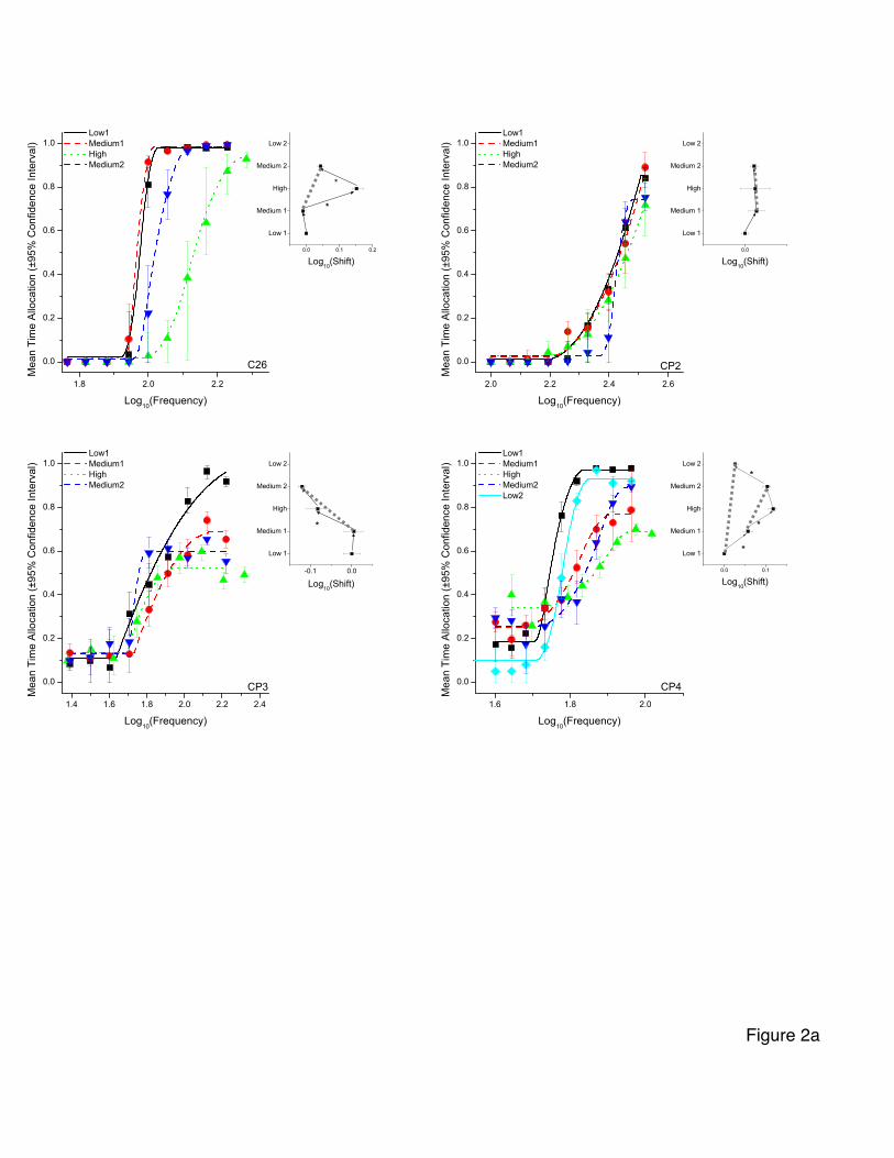
,-./01+!

2/34

,-./01+$

()*+$

,-56+7/1-+899):5;/)6+<=>?@+A)6B/.-6:-+C6;-DE59F

()3!%<GD-H0-6:IF

+()*!

+,-./01!

+2/34

+,-./01$

()3!%<J4/B;F

!

K

A$'

!"# !"! !"$ !"%

#"#

#"!

#"$

#"%

#"&

'"#

#"#

()*+'

,-./01+'

2/34

,-./01+!

()*+!

,-56+7/1-+899):5;/)6+<=>?@+A)6B/.-6:-+C6;-DE59F

()3'#<GD-H0-6:IF

+()*'

+,-./01'

+2/34

+,-./01!

AJ!

()3'#<K4/B;F

!"# !"$ !"% &"' &"& &"#

'"'

'"&

'"#

'"$

'"%

!"'

('"! '"'

)*+,!

-./012,!

3045

-./012,&

)*+,&

-.67,802.,9::*;6<0*7,=>?@A,B*7C0/.7;.,D7<.EF6:G

)*4!'=HE.I1.7;JG

,)*+!

,-./012!

,3045

,-./012&

BKL

)*4!'=M50C<G

!

!"# !"$ %"&

&"&

&"%

&"'

&"#

&"$

!"&

&"& &"!

()*+!

,-./01+!

2/34

,-./01+%

()*+%

,-56+7/1-+899):5;/)6+<=>?@+A)6B/.-6:-+C6;-DE59F

()3!&<GD-H0-6:IF

+()*!

+,-./01!

+2/34

+,-./01%

+()*%

AJ'

()3!&<K4/B;F

!

!

!

Figure 2a

!"# !"$ %"& %"%

&"&

&"%

&"'

&"#

&"$

!"&

(&"! &"&

)*+,!

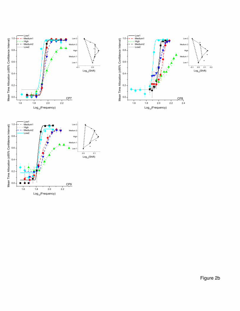
-./012,!

3045

-./012,%

)*+,%

-.67,802.,9::*;6<0*7,=>?@A,B*7C0/.7;.,D7<.EF6:G

)*4!&=HE.I1.7;JG

,)*+!

,-./012!

,3045

,-./012%

,)*+%

BKL

)*4!&=M50C<G

!

!

N

!

!"# !"$ %"& %"% %"'

&"&

&"%

&"'

&"#

&"$

!"&

(&"! &"& &"! &"%

)*+,!

-./012,!

3045

-./012,%

)*+,%

-.67,802.,9::*;6<0*7,=>?@A,B*7C0/.7;.,D7<.EF6:G

)*4!&=HE.I1.7;JG

,)*+!

,-./012!

,3045

,-./012%

,)*+%

BK$

)*4!&=L50C<G

!

!

!

!

!"# !"$ %"& %"%

&"&

&"%

&"'

&"#

&"$

!"&

&"& &"!

()*+!

,-./01+!

2/34

,-./01+%

()*+%

,-56+7/1-+899):5;/)6+<=>?@+A)6B/.-6:-+C6;-DE59F

()3!&<GD-H0-6:IF

+()*!

+,-./01!

+2/34

+,-./01%

+()*%

AJ>

()3!&<K4/B;F

!

!

!

!

Figure 2b

!"#$ "#" "#$

%&'()*+

%&'()*,

%&'()*-

%&'()*.

%&'()*$

$#, $#/ $#0 .#"

"#"

"#.

"#,

"#/

"#0

$#"

123$"45&6789

:)';*<6=)*>??2@'862;*4AB+C*D2;76E);@)*F;8)GH'?9

123$"4IG)JK);@L9

*%&'()*$

*%&'()*.

*%&'()*-

*%&'()*,

*%&'()*+

MN.

!"!

#$%&'()

#$%&'(*

#$%&'(+

#$%&'(,

#$%&'(-

)", )". )"/ *"! *"*

!"!

!"*

!",

!".

!"/

)"!

012)!34$5678

9'%:(;5<'(=>>1?%751:(3@A-B(C1:65D':?'(E:7'FG%>8

012)!3HF'IJ':?K8

(#$%&'()

(#$%&'(*

(#$%&'(+

(#$%&'(,

(#$%&'(-

LM+

!"# !"$ %"& %"% %"'

&"&

&"%

&"'

&"#

&"$

!"&

(&"! &"& &"!

)*+,-.!

)*+,-.%

)*+,-./

)*+,-.'

)*+,-.0

1-+2.345-.67789+:482.;<=0>.?82@4A-29-.B2:-CD+7E

F8G!&;HC-IJ-29KE

.)*+,-.!

.)*+,-.%

.)*+,-./

.)*+,-.'

.)*+,-.0

LM'

F8G!&;N*4@:E

!"# !"$ !"% &"' &"&

'"'

'"&

'"#

'"$

'"%

!"'

('"! '"'

)*+,-.!

)*+,-.&

)*+,-./

)*+,-.#

)*+,-.0

1-+2.345-.67789+:482.;<=0>.?82@4A-29-.B2:-CD+7E

F8G!';HC-IJ-29KE

.)*+,-.!

.)*+,-.&

.)*+,-./

.)*+,-.#

.)*+,-.0

LMN

F8G!';O*4@:E

!"#$ "#"

%&'()*$

%&'()*+

%&'()*,

%&'()*-

%&'()*.

$#/ $#0 +#" +#+ +#-

"#"

"#+

"#-

"#/

"#0

$#"

123$"45&6789

:)';*<6=)*>??2@'862;*4AB.C*D2;76E);@)*F;8)GH'?9

123$"4IG)JK);@L9

*%&'()*$

*%&'()*+

*%&'()*,

*%&'()*-

*%&'()*.

MN$

Figure 3

0.0

0.2

0.4

0.6

0.8

1.0

0.0

0.2

0.4

0.6

0.8

1.0

0.0

0.2

0.4

0.6

0.8

1.0

0.0

0.2

0.4

0.6

0.8

1.0

0.0

0.2

0.4

0.6

0.8

1.0

0.0

0.2

0.4

0.6

0.8

1.0

0.0

0.2

0.4

0.6

0.8

1.0

C26

Frequency Price

*

Fitte

d Ti

me

Allo

catio

n(±

95%

Boo

tstra

p C

onfid

ence

Inte

rval

)

CP2

*

CP3

*CP4

*

CP7 * CP8*

CP9*

!"#!"$

!"%&"!

&"'&"#

&"$ &"%

'"!

'"'

'"#!"!

!"'

!"#

!"$

!"%

&"!()*+,-+./0(12++3

(4*5/+(12++3

(673+/8+9(5.8+*1+/85:.

)588+9(;5<+(=>>:/?85:.

@ABCD(E::818*?3(F:.G59+./+(H.8+*I?>J

K:L()*+,-+./0(@MNJK:L(4*5/+(@1+/1O*+2?*9J

F'$

Figure 4

!"# !"$ !"% &"' &"& &"# &"$

'"'

'"&

'"#

'"$

'"%

!"'

'"' '"! '"& '"( '"# '") '"$

*+,

-./012

3045

-.678902.8:;;+<6=0+78>?@)A8B+7C0/.7<.8D7=.EF6;G

*+4!'>HE.I1.7<JG

8*+,

8-./012

83045

B&$

8K67/+2

8L,..M

8

*+4!'>L50C=G

!

!

!"# !"$ %"&

&"&

&"%

&"'

&"#

&"$

!"&

&"& &"! &"% &"( &"'

)*+

,-./01

2/34

,-5678/1-79::*;5</*67=>?@A7B*6C/.-6;-7D6<-EF5:G

)*3!&=HE-I0-6;JG

7)*+

7,-./01

72/34

BK'

7L56.*1

7M+--N

7

)*3!&=M4/C<G

!

!"# !"$ !"% &"' &"& &"# &"$

'"'

'"&

'"#

'"$

'"%

!"'

'"' '"! '"&

()*

+,-./0

1.23

+,4567.0,6899):4;.)56<=>?@6A)5B.-,5:,6C5;,DE49F

()2!'<GD,H/,5:IF

6()*

6+,-./0

61.23

AJK

6L45-)0

6M*,,N

6

()2!'<M3.B;F

!

!

!"# $"% $"$

%"%

%"$

%"&

%"'

%"#

!"%

%"% %"! %"$ %"(

)*+

,-./01

2/34

,-5678/1-79::*;5</*67=>?@A7B*6C/.-6;-7D6<-EF5:G

)*3!%=HE-I0-6;JG

7)*+

7,-./01

72/34 BK#

7L56.*1

7M+--N

7

)*3!%=M4/C<G

!

!

!"# !"$ !"% !"& #"' #"# #"$ #"%

'"'

'"#

'"$

'"%

'"&

!"'

('"! '"' '"! '"# '")

*+,

-./012

3045

-.678902.8:;;+<6=0+78>?@AB8C+7D0/.7<.8E7=.FG6;H

*+4!'>IF.J1.7<KH

8*+,

8-./012

83045

CL@

8M67/+2

8N,..O

8

*+4!'>N50D=H

!

!

Figure 5

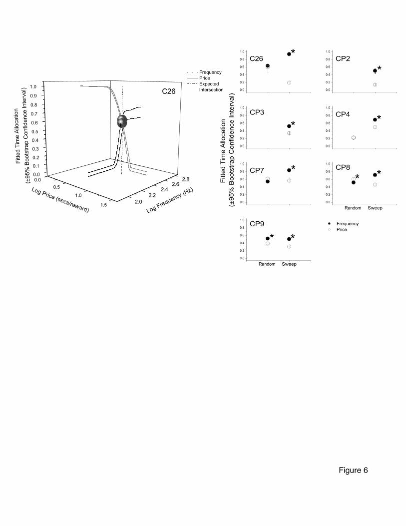
0.00.5

1.0

1.5

0.0

0.1

0.2

0.3

0.4

0.5

0.6

0.7

0.8

0.9

1.0

2.02.2

2.42.6

2.8

Frequency Price Expected

Intersection

!"##$

%&'"

($&

)**+

,-#"+

.

/012

3&4

++#5

#6-7&

8+.

9"%$.

,$&:.

#$6;

-*<

=+>& !6$?@$.,A& /BC<=+>& D6",$& /5$,5E6$F-6%<

C26 0.0

0.2

0.4

0.6

0.8

1.0

0.0

0.2

0.4

0.6

0.8

1.0

0.0

0.2

0.4

0.6

0.8

1.0

Random Sweep0.0

0.2

0.4

0.6

0.8

1.0

Random Sweep0.0

0.2

0.4

0.6

0.8

1.0

0.0

0.2

0.4

0.6

0.8

1.0

0.0

0.2

0.4

0.6

0.8

1.0*C26

FrequencyPrice

CP4 *

* *CP7

* *CP9

Fitte

d Ti

me

Allo

catio

n(±

95%

Boo

tstra

p C

onfid

ence

Inte

rval

)

*CP8

*CP3

*CP2

Figure 6

Table 1

Rat Medium HighC26 3.16 10.00CP2 2.50 6.30CP3 2.80 7.90CP4 3.20 10.00CP7 4.00 16.00CP8 4.00 16.00CP9 2.90 8.40

Price values of medium- and high-price frequency sweeps (seconds/reward)

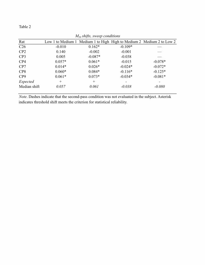
Table 2

Rat Low 1 to Medium 1 Medium 1 to High High to Medium 2 Medium 2 to Low 2C26 -0.010 0.162* -0.109* —CP2 0.140 -0.002 -0.001 —CP3 0.005 -0.087* -0.038 —CP4 0.057* 0.061* -0.015 -0.078*CP7 0.014* 0.026* -0.024* -0.072*CP8 0.060* 0.084* -0.116* -0.125*CP9 0.061* 0.073* -0.034* -0.081*Expected + + - -Median shift 0.057 0.061 -0.038 -0.080

M50 shifts, sweep conditions

Note. Dashes indicate that the second-pass condition was not evaluated in the subject. Asterisk indicates threshold shift meets the criterion for statistical reliability.

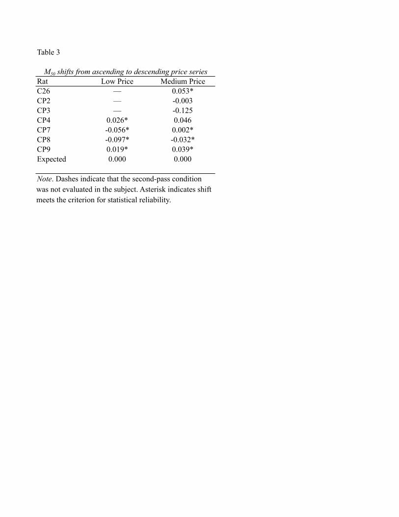
Table 3

Rat Low Price Medium PriceC26 — 0.053*CP2 — -0.003CP3 — -0.125CP4 0.026* 0.046CP7 -0.056* 0.002*CP8 -0.097* -0.032*CP9 0.019* 0.039*Expected 0.000 0.000

Note. Dashes indicate that the second-pass condition was not evaluated in the subject. Asterisk indicates shift meets the criterion for statistical reliability.

M50 shifts from ascending to descending price series

Table 4

Rat 1 to 2 2 to 3 3 to 4 4 to 5DE1 -0.028* 0.014 0.017 -0.048*DE2 -0.014 -0.009 0.046* 0.013DE3 -0.034* 0.003 0.021* 0.009DE4 0.035* -0.105* 0.052* 0.008DE7 -0.038* -0.046* 0.014* -0.003Expected 0.000 0.000 0.000 0.000Median shift -0.028 -0.009 0.021 0.008

M50 shifts, phases of drift control

Note. Asterisk indicates threshold shift meets the criterion for statistical reliability.

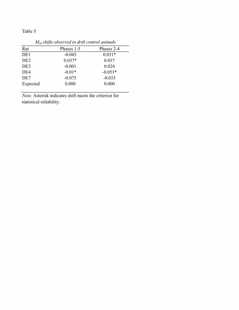
Table 5

Rat Phases 1-5 Phases 2-4DE1 -0.045 0.031*DE2 0.037* 0.037DE3 -0.001 0.024DE4 -0.01* -0.053*DE7 -0.075 -0.033Expected 0.000 0.000

M50 shifts observed in drift control animals

Note. Asterisk indicates shift meets the criterion for statistical reliability.

Table 6

UDrift control Experimental

1 to 2 / Low 1 to Medium 1 3.80 (5) 8.43 (7) 4.00*2 to 3 / Medium 1 to High 4.20 (5) 8.14 (7) 6.00*3 to 4 / High to Medium 2 10.00 (5) 4.00 (7) 0.00*4 to 5 / Medium 2 to Low 2 7.00 (5) 2.50 (4) 0.00*

Note. Asterisks indicate a statistically significant difference in magnitude of shift between drift control and non-drift control animals, p<0.05, one-tailed.

Non-parametric test of difference in price-related shifts between experimental and drift control subjects

Mean rank (n)Shift

Table 7

Rat Low to Medium Medium to HighC26 0.119* 0.413*CP4 0.119* 0.075CP7 0.083* 0.116*CP8 0.137* 0.103*CP9 0.184* 0.129*Median Shift 0.124 0.123

Note. Asterisk indicates shift meets criterion for statistical reliability.

M50 shifts, randomized conditions