raTjectory racTking Controller for a 4-DoF Flexible … · raTjectory racTking Controller for a...

Trajectory Tracking Controller for a 4-DoF Flexible Joint Robot Arm

Dimitar Ho Viktor KisnerTU Darmstadt TU Darmstadt

Abstract

In this paper, we present a trajectory track-ing controller for the �exible joint robot armBioRob. The controller compensates grav-ity and stiction torques with a feedforwardpart and joint and motor angle tracking er-rors with a linear feedback part. In orderto parametrize the controller, system identi-�cation methods have been designed to esti-mate the gravity vector, elastic transmissionand stiction model. We show that the pro-posed trajectory tracking controller outper-forms other control laws on the BioRob sys-tem in terms of the overall RMS trajectorytracking error.

1 Introduction

Flexible joint robot arms come with elastic elementsincorporated in their transmission devices. A typicalexample of such robots is the BioRob arm, see Fig-ure 1. It is a lightweight robotic manipulator withfour revolute joints coupled with actuators by elastictransmission devices, which consist of cables, pulleysand translational springs.

BioRob's joint �exibility has proven bene�cial forsafety in close human interaction, as the robot linksare inertially decoupled from the actuators. Therefore,the robot links have a lower kinetic energy in case ofan accidental collision with a human. Another advan-tage involves the ablility to store potential energy inthe translational springs, allowing for peak velocitiesin throwing tasks.

On the other hand, joint �exibility introduces greatchallenges in modeling, identi�cation and control ofthe arm. From the viewpoint of system theory, the

Figure 1: BioRob, a �exbile joint robot with four revo-lute joint. Its joint �exibility comes from elastic trans-mission devices consisting of pulleys, cables, and in-corporated springs.

elastic transmission devices double the manipulator'ssystem order. Since they furthermore exhibit a nonlin-ear behaviour and, particularly, the actuators involvefriction, a highly complicated model is required to de-scribe BioRob's dynamics. To identify the parametersof the model only data from rotary encoders on mo-tors and joints and current sensors in motors are avail-able. As the robot links are inertially decoupled fromthe actuators, BioRob poses an underactuated system,which means that the manipulator is no longer capa-ble to follow arbitrary trajectories in the con�gurationspace. As a result, oscillations of the robot links thatoccur due to the joint �exibility are very di�cult todamp.

In this paper we address the trajectory tracking prob-lem for the BioRob arm. We adapt a control algorithmpresented in [1], which combines a modelbased feedfor-ward control signal with a linear full state feedback. Tocompensate for friction we add an additional feedbackpath to the control algorithm, which is endowed with ahysteresis to avoid chattering phenomena. The controlalgorithm is designed using a mathematical model pre-sented in [2] that describes BioRob's dynamics in theso-called joint space. To identify the necessary modelparameters we have applied system identi�cation ap-


proaches, which we have customized for the BioRobarm.

The remainder of this paper is organized as follows:The BioRob arm and its dynamical equations are pre-sented in Section 2. The control algorithm for tra-jectory tracking is derived in Section 3. In Section 4we introduce a special procedure to identify all sys-tem parameters used in the control algorithm. Theperformance of our control algorithm is evaluated incomparision with other control laws in Section 5. Sec-tion 6 summarizes and re�ects results of our proposedcontroller. The Appendices A and B show open prob-lems regarding BioRob's hardware and software, aswell as other related work that has been done duringthis project.

2 Dynamical System

We begin with a concise descripton of the BioRob arm.Afterwards we introduce two di�erent sets of general-ized variables to facilitate the description of BioRob'sdynamics. Finally we present BioRob's equations ofmotion in the end of this section. For a more detailedanalysis the reader is referred to [2].

2.1 System Description

The BioRob arm shown in Figure 1 is a lightweight�exible joint robot. It has four revolute joints coupledwith electrical actuators by cable and pulley mecha-nisms. The cables have built-in translational springscausing joint �exibility. The pulleys are mounted onjoints and actuators. The electrical actuators consistof DC-motors and reduction gears. To reduce the in-ertia of the robot links they are placed near the baseof the manipulator. That is, the actuators of the �rstand second joint are attached to the �rst link, whereasthese of the third and fourth joint are on the secondlink of the arm. Since the actuator of the fourth joint islocated on the second link, an idler pulley is necessaryto drive the fourth joint. This introduces a kinematiccoupling between the third actuator and joint anglesand the fourth joint angle, what is made precise later.On BioRob's �fth link an end e�ector consisting of asmall DC motor with a gripper is mounted, which forexample may carry a table tennis racket. However,this degree of freedom is not used in this work. Forsensing its position BioRob has rotary encoders on theDC motors and joints with a resolution of 11 and 12bits. Additionally, the DC motors are equipped withcurrent sensors.

2.2 Actuator and Joint Space

For dynamic analysis, two di�erent sets of generalizedvariables are introduced, which form the so-called ac-tuator and joint space. The joint space is of particu-lar interest, as it allows for writing BioRob's dynamicequations in a more transparent manner.

The actuator space consists of the coordinates eθand eq. The coordinates eθ pose physical quantities,namely the motor angles as re�ected through the re-duction gears to the actuator side pulleys. Contrarily,the coordinates eq are virtual quantities, which can beunderstood as the joint angles re�ected through theelastic transmission devices to the actuator side pul-leys.

Similarly, in the joint space jθ and q denote generalizedcoordinates. The joint angles q are physical quantities,whereas the actuator angles jθ are virtual quantitiesre�ected through the elastic transmission devices tothe joint side pulleys.

The transformation matrix that re�ects the actuatorangle into joint space is given by

Jt =

r1R1

0 0 0

0 r2R2

0 0

0 0 r3R3

0

0 0 − r3R4

r4d3R4

r4R4

, (1)

where the diagonal elements are the conversion ratesof the cable pulley mechanisms. ri and Ri denote theradii of the �rst joint's actuator and joint side pulley.The non diagonal form is a result of the kinematiccoupling between the third and fourth joint. Thereby,the radius of the idler pulley is denoted by r4d3. Thetransformation matrix is derived for the case when thesprings exhibit their prestretched length and force. Anillustrative derivation of the transmission matrix canbe found in [2].

In terms of equations the transformation of the actu-ator angle into joint space is given by

jθ = Jteθ (2)

and, conversely, the joint angle is re�ected into theactuator space by

eq = J−1t q . (3)

Due to BioRob's joint �exibility the actuator anglere�ected into joint space jθ does normally not coincidewith the joint angle q and, vice versa, the joint angleviewed in the actuator space eq is not the same as theactuator angle eθ. Nevertheless the de�nition of thejoint and actuator space allows for interpreting thedi�erences of the angles as the de�ections of virtual

Dimitar Ho, Viktor Kisner

torsional springs, placed at the corresponding jointsor actuators.

Additionally, we de�ne the generalized torques in bothspaces, which are applied about the axes of the gener-alized coordinates. In the actuator space they are de-noted by eτm and τe. The former act about eθ and canbe perceived as the physical actuator torques, as theyare the motor torques re�ected through the reductiongears. The latter act about eq and are measureableas the torques of the elastic transmission devices onthe actuators. They can also be visualized as torquesexterted on joints by virtual torsional springs, whichare re�ected through the transmission devices. There-fore, the transformation matrix can be derived withthe principle of virtual work [2].

In a similar fashion, the torques for the joint spaceare de�ned as jτm and jτe. While jτm act about jθand are viewed as re�ected actuator torques, jτe actabout q and have the meaning of torques between twoadjacent links that are exerted from virtual torsionalsprings directly placed in the corresponding joints.

The relation between the torques of both spaces is de-scribed by

jτm = J−Tt

eτm (4)

jτe = J−Tt

eτe (5)

where J−Tt denotes the inverted and transposed matrix

Jt. The di�erence between the coordinates of the jointspace jθ − q can be interpreted as the de�ection ofvirtual torsional springs with the spring torques jτeacting between the links of the corresponding joints.As a result, the joint space allows to model BioRob asa rigid link robot with series elastic actuators placedin the joints.

2.3 Robot Dynamics

Next, we will present the Lagrangian equations ofBioRob in the joint space. To do so, three assump-tions are made, see [2] and [3]. First, it is assumedthat the center of mass of each actuator is on its ro-tation axis. In this case, the gravitational potentialenergy is independent of the actuator angles. Second,it is assumed that the kinetic energy of each actuatorrotor is due only to its own spinning, implying thatgyroscopic e�ects are neglected. Third, the kinetic en-ergy of the cables and springs is also assumed to benegligable.

The dynamics of the BioRob arm in joint space are

given by the following set of equations

jImj θ̈ + jDm

j θ̇ + jτe + jτs = jτm (6)

M(q) q̈ + C(q, q̇) q̇ + D q̇ + g(q) = jτe (7)

jτk(jθ − q) + jτd(j θ̇ − q̇) = jτe (8)

where Equations (6) and (7) describe the actuator androbot link dynamics. Equation (8) illustrates the elas-tic actuator torques, which are torques transmittedfrom the actuator to the joint side. With jIm andjDm we denote the actuator rotor inertia and damp-ing matrix. The matrices M(q), C(q, q̇) and D denotethe link inertia, the Coriolis and centripetal and thedamping matrix, while g(q) denotes the gravity vec-tor. By jτk and jτd we represent the elastic actuatorsti�ness and damping vectors. jτs and

jτm denote thefriction and the motor torque vectors, which are non-conservative generalized forces. Note, that the abovementioned parameters with a superscripted j are re-�ected to the joint space.

The synthesis of the control algorithm is based on theterms jτk(jθ− q), g(q) and jτs of the robot's dynamicequations, which are spelled out in the following. Theelastic actuator sti�ness vector can be rewritten as

jτk(jθ − q) = J−Tt RFk(RJ−1

t (jθ − q)) (9)

where Fk denotes a vector function with the physicalspring characteristics. The matrix R which consists ofthe joint side pulley radii is given by

R = diag(r1, r2, r3, r4) (10)

with diag standing for diagonal form. The argument ofthe spring force vector RJ−1

t (jθ−q) is the elongationof the translational cable springs. RFk(·) representsthe elastic actuator input torques with respect to theelastic actuator space eτe, when

jτd(j θ̇−q̇) is negligableor the robot does not move.

The gravitational torques in joint space are given by

g(q) =

s1 c1 s1s2 s1s23 s1s2340 0 c1c2 c1c23 c1c2340 0 0 c1c23 c1c2340 0 0 0 c1c234

−β1β2β3β4β5

(11)

whereas the letters s and c abbreviate the functions sinand cos. The letters' indexed numbers denote the sumof joint angles used as arguments, i.e. s23 stands forsin(q2 + q3). The parameters βi denote gravitationalterms, which will be estimated in Section 4.

In BioRob's equations of motion friction is only con-sidered in the actuator dynamics. This coincides withthe observation that the most friction is exerted in


the transmission devices of the actuators, whereas thefriction in the joints and the joint side pulleys is negli-gible. The friction with respect to the actuator spaceis modeled by a piecewise vector function as follows

eτs =

{sgn(eτext) min(|eτext|, eτ̂s(eσ)) |eθ̇| = 0

sgn(eθ̇) eτ̂s(eσ) |eθ̇| 6= 0

(12)

where sgn and min are vector functions with the signof each component of the argument and the minimumof each argument's component. At rest, the frictionacts opposite to the external torque and is given by

eτext = eτm − eg . (13)

Furthermore, we model the friction's absolute valueeτ̂s(

eσ) > 0 to depend on the torsional stress in theactuator joints eσ, which we model as

eσ = eg, (14)

since the gravity causes the main torsional joint stressat any resting position of the robot. Notice, that eg isthe gravity re�ected to the actuator space, i.e. JT

t g(q).Approximations of the vector function eτ̂s(

eσ) will bederived from static experiments, which will be pre-sented in Section 4. In motion, friction opposes theactuators' angular velocity with the value of the stic-tion function.

3 Control Algorithm

Given BioRob's dynamic equations we propose a con-trol algorithm for tracking a desired link trajectory qd.It combines a modelbased feedforward and a linear fullstate feedback similar to [1]. An overview of the con-trol algorithm is illustrated in Figure 2.

In the following derivation we assume that we onlyknow the terms jτk(jθ− q), g(q) and jτs of the robot'sdynamic equations. We also assume that the desiredlink trajectory qd is at least thrice di�erentiable.

We begin the derivation of the trajectory tracking con-troller by specifying a desired trajectory for the fullstate space consisting of q, q̇, jθ and j θ̇. As a de-sired link trajectory qd is already provided it remainsto obtain a desired motor trajectory, which will be de-noted by jθd. It has to be consistent with qd in termsof the dynamic equations. Thereto it is obtained byrearranging Equation (7) as

jθd = jτk−1(M(qd) q̈d + C(qd, q̇d) q̇d+ (15)

D q̇d + g(qd)) + qd

where the spring damping jτd is neglected. SinceM(qd), C(qd, q̇d) and D are unknown we approximatejθd with

jθd = qd + jτk−1(g(qd)) (16)

what coincides with Equation (15) for constant trajec-tories.

Next, we design the feedforward control. Its task is tomaintain BioRob roughly along the desired trajectory.If all terms of the dynamic equations are known thefeedforward control can easily be determined with theinverse dynamics algorithm

jτmd= jIm

j θ̈d + jDmj θ̇d + jτk (17)

which is obtained by inserting qd and jθd in Equation(6). The received jτmd

denotes the computed torque.However, according to the assumptions the parametersjIm and jDm are unknown. We approximate Equation(17) by

jτmd= jτk, (18)

which can be tansformed into

jτmd= g(qd) (19)

by inserting the approximated desired motor trajec-tory from Equation (16). Due to the approximationthe feedforward only compensates the gravity loadalong the desired joint trajectory. It should be notedthat the above simpli�cations are exact in case of con-stant trajectories.

Due to the above approximations the computed torqueis not su�cient to steer BioRob along the desired tra-jectory. To cope with the trajectory error, i.e. thedi�erence between the desired and the current trajec-tory, a full state feedback is necessary. Its task is tostabilize the robot along the reference trajectory. Inthis work a linear full state feedback compensator isapplied. Altogether with the computed torque fromEquation (19) the control algorithm is given by

jτm = KPq (qd − q) + KDq̇ (q̇d − q̇) + (20)

KPθ (jθd − jθ) + KDθ̇(j θ̇d − j θ̇) + g(qd),

where KPq and KPθ are proportional and KDq̇ andKDθ̇

derivative diagonal gain matrices. For setpointtracking a stability proof using a Lyapunov argumentand LaSalle's invariance theorem is given by [1].

The transmission devices of BioRob's actuators ex-ert signi�cant friction, which causes a poor trackingperformance, when not considered in the control al-gorithm. Therefore, the control algorithm, Equation(20), is augmented with an additional feedback signalto alleviate friction. Its design is based on the frictionmodel proposed in Equation (12). The friction com-pensation is determined in actuator space and for eachactuator seperately using automata as depicted in Fig-ure 3. The automata consist of four di�erent states s1,


Trajectory

Planning

jτmd

PDq

PDθ

jτms

++

+ +

BioRob[qTd q̇

Td ]

T

[jθTdj θ̇Td ]

T

jτm

qd

−

[qT q̇T]T

−

[jθT j θ̇T]T

Figure 2: Control algorithm for trajectory tracking. In the beginning of the control task a trajectory for all statevariables is planned, i.e., the actuator and joint angles and velocities. Thereafter, a gravity compensation jτmd

,a linear full state feedback PDq and PDθ, and an additional nonlinear feedback jτms

to alleviate friction is usedto track the desired trajectory.

s1

s3

s4

s2

eθ̇i < εθi

eθ̇i ≤ −δi eθ̇i > δi

|eθ̇i| ≥ εθi, ei > εei

|eθ̇i| ≥ εθi, ei < εei

|eθ̇i| ≥ εθi, ei ≤ |εei|

eθ̇i > δi

eθ̇i < −δi

Figure 3: Automaton for friction compensation withhysteresis. The friction compensation torque for eachactuator depends on the state of the corresponding au-tomaton. The automaton consists of four states con-nected by edges with assigned transition conditions. Ifno transition condition is true, the automaton remainsin the current state.

s2, s3 and s4. When the angular velocity of the corre-sponding actuator eθ̇i is below the very small thresholdεθi, its assigned automaton takes the state s1. Thenthe actuator merely moves and the additional torqueof the friction compensation

eτmsi = |eτ̂s(eg)| sat1(ei/εei) (21)

acts into the direction of the error between the desiredand the current acutator position

ei = eθdi − eθi , (22)

whereas the direction is determined using the satura-tion function

sat1(x) =

{sgn(x) |x| ≥ 1

x |x| < 1(23)

instead of a sgn function to avoid jumps in the actuatortorque. It is also possible to determine the direction ofstiction by using the external torque, as it is describedin the friction model (12). Since, however, the torquefrom the PD controller for the actuator angle is veryhigh in relation to the gravity torque, it is negligable.When eθi is above the threshold εθi the automatonchanges into state s2, s3 or s4 depending on the errorei. Contrariwise, if

eθi drops below εθi the automatonchanges back into s1. In state s2 the additional torqueis

eτmsi = |eτ̂s(eg)| sat1(eθ̇i/δi) . (24)

The automaton changes into this state when the normof the error, Equation (22), is below the thresholdεei. If the error is above or below εei the automatonchanges from s1 into state s3 or s4. In s3 the frictioncompensation torque is chosen as

eτmsi = |eτ̂s(eg)| sat2(eθ̇i/δi) (25)


whereby the direction is determined using the actuatorvelocity with function sat2 de�ned as

sat2(x) =

1 x ≥ 0

2x+ 1 −1 < x < 0

−1 x ≤ −1

. (26)

The friction compensation in state q4 is nearly thesame as in state q3, however, only sat3 given by

sat3(x) =

1 x ≥ 1

2x− 1 0 < x < 1

−1 x ≤ 0

(27)

is used instead of sat2. The automaton changes be-tween s3 and s4 depending on the actuator velocity.If it is beneath −δi the automaton changes from s3into s4. Contrariwise, the automaton takes s4 from s3when eθ̇i > δi is true. The functions sat2 and sat3 forma saturation function with hysteresis to avoid jumpsin the friction compensation. When the friction com-pensation is calculated it has to be transformed intojoint space with matrix J−T

t for the control algorithm.The parameters εθi, εei, and δi are tuning parameters,whereas εθi should always be smaller than δi.

4 System Identi�cation

As mentioned before in Section 3, we assume theknowledge of jτk(jθ − q), g(q) and jτs. The goal ofthis section will be to demonstrate the process and re-sult of the estimation of those terms. The essentialsystem parameters we have to �nd out are the valuesof Jt, R, βi, and the vector functions eτ̂s(

eσ) and Fk.

4.1 Geometric System Parameters

For computing the matrices Jt and R shown in Equa-tion (1) and (10), we measured out the radii of thedi�erent pulleys in the robotic system. The results ofthe measurements are noted in the following table:

r1 0.0079 mr2 0.0121 mr3 0.0121 mr4 0.0090 mR1 0.0245 mR2 0.0403 mR3 0.0306 mR4 0.0250 mr4d3 0.0120 m

Table 1: Geometric system parameters of BioRob.

4.2 Identi�cation of NonlinearForce-Elongation Curves of SpringSystem

Calculating the desired motor trajectory jθd fromEquation (16), we need exact knowledge of the vec-tor function Fk and it's inverse. Due to our modelingof the elastic forces between the motor and the jointsas (9), Fk takes the decoupled form

Fk(x) =

fk1(x1)fk2(x2)fk3(x3)fk4(x4)

(28)

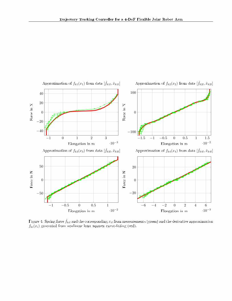
where fki(xi) and xi are the force-elongation func-tions and the physical elongation of the spring systemin joint i respectively. Using the measurementmechanism as shown in Figure 6 we will show inthe following, how we can estimate the functionsfki through measuring a set of discrete points andusing curve-�tting techniques to compute functionapproximations.

The measurement procedure is performed as follows.Firstly, the robot arm is being controlled with a PID-controller

jτm = jτPID (29)

= Kp (q0 − q)−Kd q̇ + Ki

∫ t

0

(q0 − q(τ))dτ (30)

to hold the hanging posture q = q0 shown in Figure6. In this position, the robot is not experiencing anygravitational torque in his joints, thus g(q0) = 0 andthe position q = q0, θ = 0 is an equilibrium point ofthe system. While the controller is still running, wecontinuously increase the weight in the plastic bowldepicted in Figure 6 and collect measurements of thede�ection (jθ− q) and weight once the PID-controllerhas controlled the robot to its original gravitation-freeposture q0. Once the bowl has reached the speci�edmaximum weight, we continue the measurements withthen decreasing the weights in the bowl. This mea-surement procedure has been performed in di�erentde�ection directions of the robot arm for measuringdi�erent springs of the system. Furthermore, the pro-cedure allows to study the eventual hysteresis e�ectin the springs. From those experiments we yield lpairs of bowl weightsml and corresponding de�ections(jθ− q0)l which we can now use to estimate the di�er-ent fki-curves.

Controlling the BioRob with PID controller togetherwith the measurement system attached, the equationsfor the equilibrium of the system can be derived using


Figure 6: This picture shows the four measurementsetups we used for performing our measurements toestimate the spring curves and the stiction model.

the Equations (6 - 9) and inserting the mechanics ofthe measurement system:

jτe + jτs = jτPID (31)jτL1/2 = jτe (32)

jτk(jθ − q0) = jτe (33)

R−1 JTtjτk(jθ − q0) = Fk(RJ−1

t (jθ − q)). (34)

Notice, that for yielding Equation (32), we used thatg(q0) = 0 and included in the original Equations (7)the term jτL1/2, which describes what torques are be-ing generated on the joints by the loads and attach-ment position of our measurement mechanism. In theactuator Equations (6), we have substituted the PID-controller to yield (31) and at equilibrium, jτPID takesa constant value coming from the I-part of the con-troller, which compensates the load and also the stic-tion forces in jτs, keeping the robot at the desired po-sition q0. Further we can eliminate Equations (32) and(33) by substituting in the other Equations (33) and

(31) and yield

jτL1/2 + jτs = jτPID (35)

R−1 JTtjτL1/2 = Fk(RJ−1

t (jθ − q)). (36)

The load torque jτL1/2 which is being generated fromthe weights, stretches the springs in di�erent joints,which can be seen in the Equation (36). This equa-tion will be the basis for our estimation of Fk andthe computation of jτL1/2 will be crucial. Nonethe-less, computing jτL1/2 through the measurable statictorque generated from the PID controller would pro-vide too inaccurate results, since as can be seen in(35) the controller not only compensates the load butalso compensates the stiction/friction component jτs,which is known to be fairly big for our robotic system.The load torque is therefore necessary to be computeddirectly from the weights and the mechanics/geometryof the measurement setup. Depending on which of theexperimental setups is chosen in Figure 6, the loadtorque jτL1/2 coming from the measurement mecha-nism takes one of the following forms:

jτL1 =

0l2g

l3g cos(α)l4g cos(α)

ml or jτL2 =

l1g000

ml

(37)

where l1 = 0.73681 m, l2 = 0.73681 m, l3 = 0.42781 m,l4 = 0.1172 m are lengths of di�erent levers with whichthe load in the bowl acts on the joints, g = 9.81m/s2 isthe gravitational constant and α = 5.1◦ is the amountof link torsion in degrees which is found on the secondlink of the robot.

Using the special form of (28), we can further split thevector Equation (36) into its index components andyield the form

(R−1 JT

tjτL1/2

)i

= fki((RJ−1

t (jθ − q))i). (38)

From each pair of bowl weights ml and correspondingde�ections (jθ − q0)l from our experiments, wecan now compute discrete values for spring forcesf̂kil =

(R−1 JT

tjτL1/2

)il

from (37) and their asso-

ciated spring elongations xil =(RJ−1

t (jθ − q0))il.

With this set of f̂kil and xil values, we can use curve-�tting methods to estimate the functions fki. Weused nonlinear least-squares method to �t polynomialfunctions to the data and yield the estimation resultspresented in Figure 4.

Notice that the measurement data displayed in Fig-ure 4 shows, that the springs corresponding to joint 1and 2 show noticeable nonlinearity. As more detailed


described in [2], the nonlinearities in fki originate par-tially from the static slacking e�ect. Other reasonsfor the nonlinear characteristic are unmodeled elastic-ities in the transmission, especially the safety stringsincorporated in the springs, which prevent the springsfrom overstretching. Those strings limit the maximumelongation of the springs and they are considered in ourapproximations in Figure (4). Furthermore we can seethat all springs show hysteresis e�ects, especially whenexperiencing higher forces.

4.3 Identi�cation of Stiction/Friction Model

As mentioned in Section 2, the controller is designed toaccount for the stiction and friction in the robot andtherefore it is necessary to estimate the vector func-tion eτ̂s(

eσ), which describes the amount of stictionand friction torque that acts on the actuator side withrespect to the static joint stress. Since this torqueis re�ected to the actuator state space, we can fur-ther assume, that the friction in a motor joint onlydepends on the stress experienced in the same motorjoint. Therefore the torque eτ̂s(

eσ) takes the decoupledform

eτ̂s(eσ) =

eτ̂s1(eσ1)eτ̂s2(eσ2)eτ̂s3(eσ3)eτ̂s4(eσ4)

. (39)

To estimate this function, we will use the samemeasurement procedure and mechanism shown inFigure 6. However, instead of measuring for eachweigth ml the de�ection, we will measure the statictorque of the PID-controller at equilibrium andcompute the load torque eτL1/2 originating from thecorresponding weights ml. The idea is, to measurea set of equilibrium torques of the PID-controller,which stabilize the system at the same load torqueeτL1/2. Computing the maximum di�erence betweenthe PID-torques and the corresponding load torque,we can approximate the maximum stiction torque forthe associated joint stress induced by the load torque.This procedure will be explained now more in detail.

Transforming the static equilibrium equations for thejoint side (35) to the actuator side and substituting ourmodel of the stiction force from (12) into the equation,we yield:

eτL1/2 + sgn(eτext) min(|eτext|, eτ̂s(eσ)) = eτPID. (40)

Because our robotic system has the measurementmechanism attached producing an additional loadtorque eτL1/2, the external torque eτext and the tor-sional stress eσ change for our experiment. The exter-nal torque is the di�erence between the PID-controller

and the load torque

eτext = eτPID − eg(q0)− eτL1/2 = eτPID − eτL1/2 (41)

and the torsional stress eσ consists only of the loadtorque re�ected to the actuator joints

eσ = eg(q0) + eτL1/2 = eτL1/2 (42)

since the gravity eg(q0) is zero in the equilibrium po-sition q = q0. Plugging (42) and (41) into Equation(40), we �nally yield

sgn(eτPID − eτL1/2) min(|eτPID − eτL1/2|, eτ̂s(eτL1/2))

= eτPID − eτL1/2 (43)

and further in index form

sgn(eτPIDi − eτL1/2i) min(|eτPIDi − eτL1/2i|, eτ̂si(eτL1/2i))= eτPIDi − eτL1/2i (44)

which describes the equilibrium of the actuator dy-namics in closed loop during the experiment. Inspect-ing the solutions of Equation (44) we get the followingpossible equilibrium states

eτPIDi − eτL1/2i = s ≤ eτ̂si(eτL1/2i) (45)

what matches with the expected behavior of thesystem at equilibrium. If at rest (eθ̇ = 0), the externaltorque is small enough to be compensated by stictionforces, hence |eτPIDi − eτL1/2i| ≤ eτ̂si(

eτL1/2i), thenthe external torque is equal to some stiction forces ≤ eτ̂si(

eτL1/2i) smaller than the maximum stictionforce. To the contrary, if the external torque exceedsthe maximum stiction force (for example when theI-Part of the controller is increasing due to q 6= q0)the Equation (44) has no solution, because thestiction can not compensate the external torque. Themotor starts moving then, leaving the equilibriumstate eθ̇ = 0. With Equation (45), we can use ourcollected measurements of eτL1/2 and eτPID pairs inthe following to provide an estimate for the functionseτ̂si(

eσi).

From Equation (45), we know in our experiment thatfor the same �x load torque τL1/2, the resulting setof equilibrium torque di�erences (eτL1/2 − eτPID) willalways be smaller then the corresponding maximumstiction eτ̂si(

eσi). Starting the robotic system from dif-ferent enough starting conditions, the PID-controllerwill produce varying �nal equilibrium torque di�er-ences (eτL1/2 − eτPID). By collecting a big enoughset of those measurements, we can explore the spanof possible equilibrium torque di�erences to a certainjoint stress eσi and approximate the maximum stictionforce eeσi = τ̂si(

eτL1/2i) by the maximum equilibrium


torque di�erence in the measurement set. Therefore,having k measurements of eτPID for a weight ml, wecan approximate eτ̂si(

eσi = eτL1/2i(ml)) through

eτ̂si(eτL1/2i(ml)) ≈ max

k|eτPIDik − eτL1/2i(ml)| (46)

Computing this approximation for various weights ml,we yield a set of l estimated points (eτ̂ sil,

eσil) which wecan again use to construct an approximate function foreτ̂si(

eσi) by curve-�tting. As a curve-�tting method weagain use nonlinear polynomial least squares and theresulting approximation together with the used mea-surement data is depicted in Figure 5. Our experi-ments show that the stiction forces in each joint in-creases with the acting joint stress. From this approx-imation of eτ̂s(

eσ), we can compute j τ̂s(eσ) through

transformation and use the function for the controldesign discussed in Section (3) to compensate for thestiction and friction torques in the robot.

4.4 Identi�cation of Gravity Vector g(q)

For estimating g(q), as seen in Equation 11, we needto identify the parameters βi. We will estimate themthrough controlling the robot to various positionswith a PID-controller and then compensating theactuator's torque through external load torque in-duced by weights and lever mechanisms attachedto the robot. So, we are compensating the gravitytorque with external and known load torques andthereby we can estimate the gravity vector at thespeci�ed positions. Using the knowledge of thespecial structure of g(q), we can use those measure-ments to further estimate the constants βi. In thefollowing we will explain this procedure in more detail.

First, we specify postures kq̂, for which the gravityvector takes a form which will make it convenient toestimate the constants βi and to attach the compen-sation weights to the robot. The di�erent posturescan be seen in Figure(7) and Figure(8), with the cor-responding weigth load attachment. Writen as vectorin joint space, those postures kq̂ are

0q̂ = [−π/2, 0, 0, 0]T

(47)

1q̂ = [0,−π/2, 0, 0]T

(48)

2q̂ = [0, 0, 0, 0]T

(49)

3q̂ = [0,−π/2, π/2, 0]T

(50)

4q̂ = [0,−π/2, 0, π/2]T

(51)

Figure 7: Postures 2q̂ (lower), 3q̂ (upper left) and 4q̂(upper right) at which we apply external torques atq2, q3 and q4 respectively, through weights and cor-responding lever mechanisms. The water bottle hasbeen used in order to be able to change the weightcontinuously.

which give the associated gravity vectors

g(0q̂) = [β1, 0, 0, 0]T

(52)

g(1q̂) = [β2, 0, 0, 0]T

(53)

g(2q̂) = [β2, β3 + β4 + β5, β4 + β5, β5]T

(54)

g(3q̂) = [β2, β4 + β5, β4 + β5, β5]T

(55)

g(4q̂) = [β2, β5, β5, β5]T

(56)

To estimate the constants βi now, we try to �nd thecorrect weight, which through our lever-mechanismshown in Figure 7 and Figure 8 is compensatingthe actuator torque in a speci�ed joint. If we aremanaging to compensate the actuator torque, whichis meant to keep the robot in the desired positionthrough our chosen weight, the load torque whichwe are applying to this joint is compensating the


Figure 8: Postures 0q̂ (lower) and 1q̂ (upper) at whichwe apply external torques in q1 through the weightand corresponding lever mechanisms. The continuousadjustment of the external torque can be achieved byadjusting the acting lever length.

gravity torque acting on this joint. With this methodwe can measure, the gravity torque acting on aparticular joint at a particular posture. To observewhen we reached the gravity compensating weight,we check if the elongation of the translational springsof the corresponding actuator is at neutral position.This is the most accurate way to determine if weare compensating the actuator torque, since we arecircumventing the in�uence of stiction, we would haveif we simply look when the controller torque turns zero.

In Figure 7 and Figure 8, we show which postures andwhich joints we chose to estimate the gravity inducedjoint torque. From the experiments in Figure 8, we

could estimate the gravity acting in q1 in the pos-ture 0q̂ and 1q̂ and thereby collected the measurementsz1 = β1 and z2 = β2 respectively. From the other ex-periment setups shown in Figure 7, we could estimatethe gravity torques acting in joint q2, q3 and q4 for thepostures 2q̂, 3q̂ and 4q̂ respectively. From those exper-iments we got the measurements z3 = β3 + β4 + β5,z4 = β4+β5 and z5 = β5. Writing the relation betweenour measurements zi and βi, we get the following linearset of equations:

z1z2z3z4z5

=

1 0 0 0 00 1 0 0 00 0 1 1 10 0 0 1 10 0 0 0 1

β1β2β3β4β5

. (57)

and solving it provides the estimations for βi as pre-sented in Table 2.

β1 β2 β3 β4 β50.1992 0.09152 0.80249 0.7541 0.1393

Table 2: Measurement Results for βi

5 Experimental Results

In this section we will demonstrate the performanceof our controller from Section 3 on the BioRob robot.To test the performance and e�cacy of our controller,we will try to track the same trajectory with di�erentcontrollers to compare how our controller manages tra-jectory tracking regarding the performances of othercontrol laws. The benchmark trajectory is generatedusing minimum jerk algorithm for a set of points andtimes of arrival and is plotted in the Figures 9- 12in blue. The desired trajectory has been designed tocover a large domain of the state space with fairly fastmotions. As shown in Figures 9 - 12, the trajecto-ries span more than π radians in each joint and coverdi�erent exposure to gravitational torque during exe-cution. The presented trajectory tracking results havebeen shown to be consistent over many iterations withthe same controller con�guration. The performanceevaluation of each controller will be based on ERMS,

ERMS =

4∑

i=1

(eqi + eθi) (58)


where eqi and eθi are the RMS trajectory errors of thecorresponding state:

eqi =

√√√√N∑

k=1

(qik − qidk)2 (59)

eθi =

√√√√N∑

k=1

(θik − θidk)2. (60)

In the following, we will show the experimental resultsof tracking the trajectory with di�erent controllers andwill compare the di�erent controller performances.

5.1 PD-Controller in q

In Figure 9, we show the trajectory tracking using aPD-controller which only uses the joint sensor infor-mation q. Thus, the control law is formulated as

jτm = KPq (qd − q) + KDq̇ (q̇d − q̇) (61)

where qd describes the desired trajectory we aretrying to follow. To achieve the results in Fig-ure 9, the controller was parametrized with KPq

=diag (20, 20, 15, 10), KDq̇

= diag (0.2, 0.2, 0.1, 0.1).Evaluating the performance of the controller we getthe RMS error values in Table (3).

eq1 0.1016 eθ1 0.1102eq2 0.2613 eθ2 0.2360eq3 0.2217 eθ3 0.1993eq4 0.2565 eθ4 0.2521

Σ 0.8412 Σ 0.7976ERMS = 1.6388

Table 3: RMS errors calculated from trajectory track-ing experiment with controller (61)

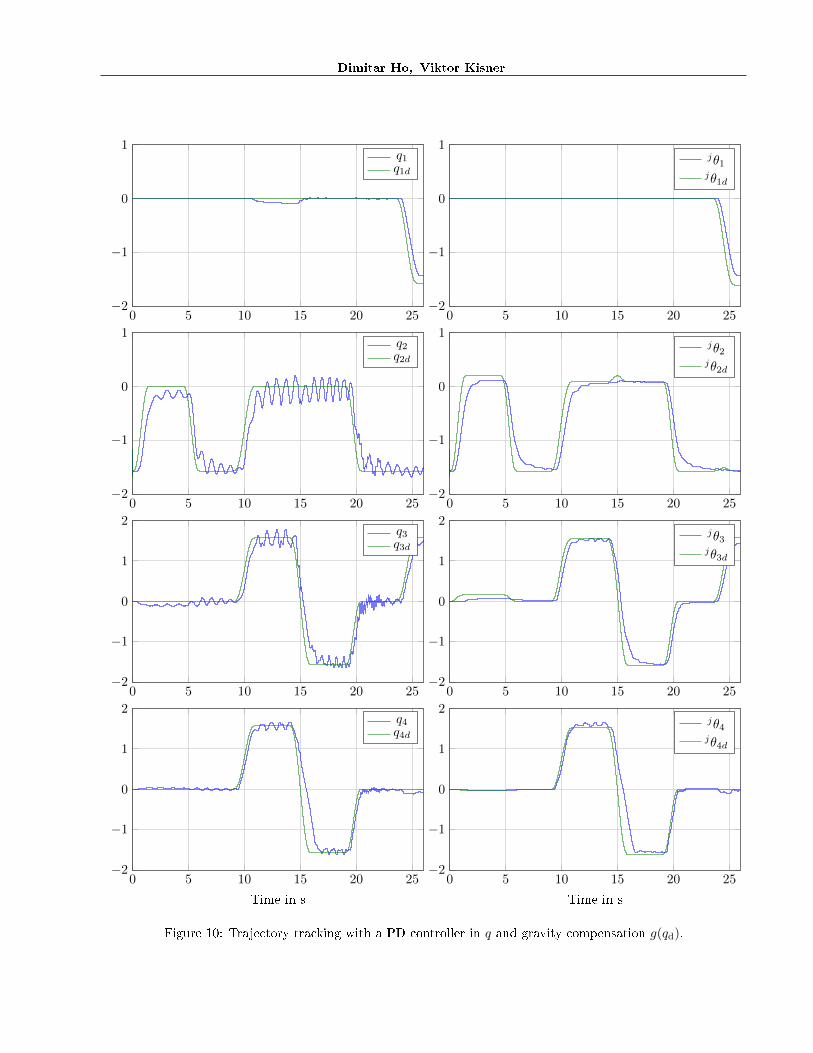
5.2 PD-Controller in q with gravitycompensation

Next, Figure 10 show the trajectory tracking using aPD-controller using only the joint sensor informationq and compensating the gravity in�uence. The con-troller is the same as in (61), but includes the termg(qd), which compensates the gravity along the desiredtrajectory of the robot qd.

jτm = KPq(qd − q) + KDq̇

(q̇d − q̇) + g(qd) (62)

To achieve the results in Figure 10, the controller wasparametrized with KPq = diag (20, 20, 15, 10), KDq̇ =diag (0.2, 0.2, 0.1, 0.1). Evaluating the performance ofthe controller we get the RMS error values in Table(4).


Σ 0.7810 Σ 0.7655ERMS = 1.5466


5.3 PD-Controller in q and jθ with gravitycompensation

The trajectory tracking performance of a PD-controller using both q and θ with gravity compen-sation g(qd) is shown in the following Figure 11. Thecontrol takes the form of our controller from Section3:


KPθ (jθd − jθ) + KDθ̇(j θ̇d − j θ̇) + g(qd)

To achieve the results in Figure 11, the controller wasparametrized with KPq = diag (1, 2, 6.5, 9), KDq̇ =diag (0, 0, 0, 0), KPθ = diag (45, 80, 80, 40), KDθ̇

=diag (0, 0, 0, 0). Evaluating the performance of the con-troller we get the RMS error values in Table (5).


Σ 0.3998 Σ 0.3658ERMS = 0.7657


5.4 PD-Controller in q and jθ with gravityand friction compensation

In this subsection we present the results of trajectorytracking using our full control algorithm of Section 3in Figure 12. In total, the controller consists of a PD-controller q and θ-wise, a gravity compensation g(qd)and a stiction compensation j τ̂s which we described inSection 3:


KPθ (jθd − jθ) + KDθ̇(j θ̇d − j θ̇) + g(qd) + j τ̂s

To achieve the results in Figure 12, the controllerwas parametrized with KPq = diag (1, 2, 6.5, 9),KDq̇

= diag (0, 0, 0, 0), KPθ = diag (45, 80, 80, 40),KDθ̇

= diag (0, 0, 0, 0). The tuning parameters


of the stiction compensation were chosen as εe =[0.001, 0.001, 0.001, 0.001] and δ = [0.1, 0.1, 0.1, 0.5].Evaluating the performance of the controller we getthe RMS error values in Table (6).


Σ 0.3848 Σ 0.3429ERMS = 0.7277


5.5 PD-Controller in jθ with gravity andfriction compensation

Since the PD-gainsKPqandKDq̇

of our �nal controllerare relatively small, we are trying to determine theirin�uence on the overall control performance in thissubsection. Therefore in Figure 13, we present theresults of trajectory tracking using the controller fromSection 5.4 but with KPq

and KDq̇set to zero, which

yields the following control law:

jτm = KPθ (jθd − jθ) + KDθ̇(j θ̇d − j θ̇) + g(qd) + j τ̂s

(65)

To achieve the results in Figure 13, the remaining pa-rameters of the controller were chosen as in Subsection5.4. Evaluating the performance of the controller weget the RMS error values in Table (7).


Σ 0.4078 Σ 0.3575ERMS = 0.7653


5.6 Comparison

Comparing the trajectory tracking of all controllerspreviously presented, we can see how our controllerimproves the performance with respect to the sim-pler control algorithms presented in Sections 5.1 -5.3. In Table (8), we can see the summary of con-troller tracking errors during the experiments and Fig-ure 14 shows a direct comparison of all controller per-formances when trying to track a trajectory in q3.

Σq Σθ ERMS

PD in q 0.8412 0.7976 1.6388PD in q + g.c. 0.7810 0.7655 1.5466

PD in q, jθ + g.c. 0.3998 0.3658 0.7657PD in jθ + g.c.+ f.c. 0.4078 0.3575 0.7653

PD in q, jθ + g.c. + f.c. 0.3848 0.3429 0.7277

Table 8: Summary of trajectory tracking errors fordi�erent control laws. (g.c. = gravity compensation,f.c. = friction compensation)

In Figure 9, we see that the controller tracks the trajec-tory with a big error, because it is not accounting forthe gravity torque acting on the joints. Furthermorethe closed loop system shows severe undamped oscil-lations. Although those oscillations still remain, usingthe PD-controller with gravity compensation in Figure10 improves the controller performance, when compar-ing the ERMS values, as seen in Table (3) and (4) ofboth controllers. In Figure 11 we notice that the os-cillations and the fairly big tracking error we observedin the previous controllers are being tremendously re-duced by adding a PD-controller in jθ in Section 5.3.We can also observe a strong decline in the RMS errorvalues (Table 5) of this experiment and see that thePD-controller in q and jθ with gravity compensationtracks the trajectories with a better accuracy. Fur-thermore we also notice, that due to stiction forces,the motor angles are slacking and are having di�cul-ties tracking the desired trajectory. This e�ect is vis-ible the most, when looking at the graphs of jθ2 andjθ3 in Figure 11. The big stiction forces acting on theactuator side of the BioRob robot prevent the robotfrom moving, until the tracking error is big enough,such that the resulting controller torque exceeds themaximum stiction force. This can be improved by in-cluding the stiction/friction compensation to our con-troller in Section (5.4). Comparing Figure 11 with 12and comparing the RMS-error (Table 5) and (Table 6)of both experiments we see that our stiction/frictioncompensation reduces the motor angle slacking of ourcontroller and thereby further reduces the tracking er-ror to the trajectories. Comparing our �nal tuningparameters of our full control law in Figure 12, we seethat the PD-gains in q are signi�cantly smaller thanthe ones of the PD-gains in jθ. By setting the PD-gains in q to zero and running another experiment, wecan see as in Figure 13, that aside from attenuatingoscillations in q2, they have little e�ect on the over-all closed loop performance of the system since theRMS error values (Table 7) barely change from (Table6). We achieved the increase in controller performancethrough our control design mostly by calculating thedesired motor position jθd correctly and implementinga high gain PD-part in jθ.


Overall, the controller performs with a strongly im-proved tracking behavior, but still shows some signif-icant oscillations in q2. The remaining tracking errorand oscillations in the closed loop system are comingmostly from the lack of knowledge of the dynamicalparameters like M(q), C(q, q̇), etc. and therefore theinability to calculate the desired trajectory of the ac-tuator jθd considering not only static but dynamic ef-fects. Furthermore, notice also in all Figure 13 to 9,the fairly big tracking errors in q1 between 10 and 15and in q4 between 13 and 17. Those originate mostlikely from problems of the electro-mechanical systemof the robot as discussed later in Section (A).

6 Conclusion

In this work, we designed a trajectory trackingcontroller for the �exible joint robot arm BioRob.The controller design is based on [1] and consists ofa PD-controller in both joint and actuator state, agravitational compensation along the desired trajec-tory and an actuator stiction compensation. For thedesign of the controller we used knowledge of thegravity vector, the force-elongation characteristicsof the springs in the transmission and the stictiontorques acting on the actuator side of the robot. Allthose parameters has been estimated by designingand performing BioRob-tailored system identi�cationmethods. Comparing the resulting controller withprevious control laws, we noticed that our controllercould drastically improve the performance of theclosed loop system.

Future work should be invested in improving thecontroller performance even more, since despite theperformance improvement, signi�cant oscillations andtracking errors are still present. In order to improvethe performance of the system, more work has to be in-vested in system identi�cation of the dynamic param-eters of the system. Furthermore, adressing the me-chanical and software problems we have encounteredduring our work would reduce the system inherent lim-its of the BioRob and allow for better control design.Particular focus should be put on trying to learn orestimate the dynamic model of the friction and stic-tion e�ects occurring in the BioRob system. Furtherimprovement of the controller performance can alsobe achieved by computing the desired actuator anglebased on the inverse dynamics computed joint torque.

References

[1] A. Albu-Schä�er and G. Hirzinger. State feedbackcontroller for �exible joint robots: a globally sta-

ble approach implemented on DLR's light-weightrobots. In Proceedings of the IEEE/RSJ Interna-tional Conference on Intelligent Robots and Sys-tems (IROS), 2:1087-1093, 2000.

[2] T. Lens, and O. von Stryk. Design and Dynam-ics Model of a Lightweight Series Elastic Tendon-Driven Robot Arm. In Proceedings of the IEEE In-ternational Conference on Robotics and Automa-tion (ICRA), pp. 4512-4518, 2013.

[3] A. De Luca and W. Book. Robots with FlexibleElements. In Springer Handbook of Robotics, B. Si-ciliano and O. Khatib, Eds. Springer Berlin Heidel-berg, pp. 287-319, 2008.


−1 0 1 2 3

·10−3

−40

−20

0

20

40

Elongation in m

Forcein

N

Approximation of fk1(x1) from data [f̂k1l, x̂k1l]

−1.5 −1 −0.5 0 0.5 1 1.5

·10−2

−100

0

100

Elongation in m

Forcein

N


−6 −4 −2 0 2 4 6

·10−3

−20

0

20

Elongation in m

Forcein

N


−1 −0.5 0 0.5 1

·10−2

−50

0

50

Elongation in m

Forcein

N


Figure 4: Spring force f̂kil and the corresponding xil from measurements (green) and the derivative approximationfki(xi) generated from nonlinear least squares curve-�tting (red).


−0.3 −0.2 −0.1 0 0.1 0.2 0.3

−0.5

0

0.5

Torsional Stress eσ1 in Nm

StictionTorquein

Nm

Approx. of eτ̂s1(eσ1) from

eτPID1k − eτL1/21(ml)

−1 −0.5 0 0.5 1 1.5

−2

0

2


StictionTorquein

Nm



−0.2 −0.1 0 0.1 0.2−0.4

−0.2

0

0.2

0.4


StictionTorquein

Nm



−0.5 0 0.5

−1

0

1


StictionTorquein

Nm



Figure 5: The measured k torque di�erences eτPIDik − eτL1/2i(ml) to the corresponding joint stress eσi =eτL1/2i(ml) ( green points), maximum absolute di�erence maxk |eτPIDik − eτL1/2i(ml)| (red) and the derivativeapproximation for the function eτ̂si(

eτL1/2i(ml)) generated from nonlinear least-squares (blue).


0 5 10 15 20 25−2

−1

0

1

2q2q2d

0 5 10 15 20 25−2

−1

0

1

2q1q1d

0 5 10 15 20 25−2

−1

0

1

2jθ1jθ1d

0 5 10 15 20 25−2

−1

0

1

2jθ2jθ2d

0 5 10 15 20 25−2

−1

0

1

2jθ3jθ3d

0 5 10 15 20 25−2

−1

0

1

2q3q3d

0 5 10 15 20 25−2

−1

0

1

2

Time in s

q4q4d

0 5 10 15 20 25−2

−1

0

1

2

Time in s

jθ4jθ4d

Figure 9: Trajectory tracking with a PD controller in q.


0 5 10 15 20 25−2

−1

0

1q2q2d

0 5 10 15 20 25−2

−1

0

1q1q1d

0 5 10 15 20 25−2

−1

0

1jθ1jθ1d

0 5 10 15 20 25−2

−1

0

1jθ2jθ2d

0 5 10 15 20 25−2

−1

0

1

2jθ3jθ3d

0 5 10 15 20 25−2

−1

0

1

2q3q3d

0 5 10 15 20 25−2

−1

0

1

2

Time in s

q4q4d

0 5 10 15 20 25−2

−1

0

1

2

Time in s

jθ4jθ4d

Figure 10: Trajectory tracking with a PD controller in q and gravity compensation g(qd).


0 5 10 15 20 25−2

−1

0

q2q2d

0 5 10 15 20 25−2

−1

0

q1q1d

0 5 10 15 20 25−2

−1

0

jθ1jθ1d

0 5 10 15 20 25−2

−1

0

jθ2jθ2d

0 5 10 15 20 25−2

−1

0

1

2jθ3jθ3d

0 5 10 15 20 25−2

−1

0

1

2q3q3d

0 5 10 15 20 25−2

−1

0

1

2

Time in s

q4q4d

0 5 10 15 20 25−2

−1

0

1

2

Time in s

jθ4jθ4d

Figure 11: Trajectory tracking with a PD controller in q and θ and gravity compensation g(qd).


0 5 10 15 20 25−2

−1

0

1

2q2q2d

0 5 10 15 20 25−2

−1

0

1

2q1q1d

0 5 10 15 20 25−2

−1

0

1

2θ1θ1d

0 5 10 15 20 25−2

−1

0

1

2θ2θ2d

0 5 10 15 20 25−2

−1

0

1

2θ3θ3d

0 5 10 15 20 25−2

−1

0

1

2q3q3d

0 5 10 15 20 25−2

−1

0

1

2

Time in s

q4q4d

0 5 10 15 20 25−2

−1

0

1

2

Time in s

θ4θ4d

Figure 12: Trajectory tracking with full controller: PD controller in q and θ with gravity compensation g(qd)and friction compensation j τ̂s.


0 5 10 15 20 25−2

−1

0

1q2q2d

0 5 10 15 20 25−2

−1

0

1q1q1d

0 5 10 15 20 25−2

−1

0

1jθ1jθ1d

0 5 10 15 20 25−2

−1

0

1jθ2jθ2d

0 5 10 15 20 25−2

−1

0

1

2jθ3jθ3d

0 5 10 15 20 25−2

−1

0

1

2q3q3d

0 5 10 15 20 25−2

−1

0

1

2

Time in s

q4q4d

0 5 10 15 20 25−2

−1

0

1

2

Time in s

jθ4jθ4d

Figure 13: PD controller in θ with gravity compensation g(qd) and friction compensation j τ̂s.


0 5 10 15 20 25−2

−1

0

1

2

PDq,θ+g.c.: q3PDq,θ+g.c.: q3d

0 5 10 15 20 25−2

−1

0

1

2

PDq: q3PDq: q3d

0 5 10 15 20 25−2

−1

0

1

2

PDq+g.c.: q3PDq+g.c.: q3d

0 5 10 15 20 25−2

−1

0

1

2

PDθ+g.c.+f.c.: q3PDθ+g.c.+f.c.: q3d

0 2 4 6 8 10 12 14 16 18 20 22 24 26−2

−1

0

1

2

PDq,θ+g.c.+f.c.: q3PDq,θ+g.c.+f.c.: q3d

Figure 14: Comparisson of performances of all controllers regarding trajectory tracking in joint q3.


A Bugs and other Problems

In this appendix, we would like to point out somepresent and unsolved problems we noticed, whichshould be adressed in future work with the BioRob.

A.1 Mechanical Problems

Taking a look at the second link of the BioRob,one can see that it is not aligned with the the restof the robot body. It is torsionally twisted by 5.1◦

with respect to its longitudinal rotational axis. Thisshould be �xed, since mostly the inverse kinematicscurrently is not considering this e�ect. Furthermore,the dynamical parameters like inertia, coriolis andcentrifugal matrices change due to this misalignment.

When trying to track fast trajectories, the ropesattached to the springs come into slacking and slipo� the pulleys. This even leads to the ropes rippingand damaging the robot. The springs of the systemhave to be either prestressed or become more sti� inorder to prevent slacking of the springs, which sofarfrequently occurs.

The mechanical elastic transmission system of the �rstjoint shows some problems, which limit the controlperformance of the robot. Firstly, the mechanicaldesign of the transmission in the �rst joint has asigni�cant deadzone of approximately 10◦ − 20◦. Onecould solve this problem by adjusting the slidingbearing, which is attached to the spring and rope.Another possibility would be to make the wholejoint completely sti�, as the region in which thetransmission is elastic, is anyway really limited.From the control theory point of view, the deadzoneinduces mechanical impacts and uncontrollabilitywhen directions are changed during a trajectory. Onecould theoretically remove the problems originatingfrom the deadzone, with a high-gain controller whichproduces high accelerations on the motorside, but thissolution is not realistic and not practical to aim for.The deadzone is also the cause for the sudden increasein tracking error in q1 between the 10 and 15 secondin Figures 13 to 9. During that time frame, the thirdlink moves and due to the torsional misalignment ofthe second link, the thereby induced and graduallyincreasing gravity torque in q1 compensates thegravity torque of link q1 and makes the �rst jointrotate to the other border of the deadzone, whichcauses the visible tracking error.

The second link of the robot (between joint q2 and

q3) is not completely rigidly attached to the metalplates it is mounted on. During fast motions in q2,the inertial forces make the link jump around 5◦− 10◦

which requires manual readjustment afterwards.

Another problem has been noted when actuating jointq4 in the negative direction. Although it is possible toachieve good tracking behavior in q4 for positive an-gles, enormous torques are needed to perform motionsin the opposite directions. This phenomena is also thereason for the big tracking errors in q4 and θ4 betweenthe 13 and 17 second in Figures 13 to 9, since the con-troller is faced more resistance when trying to movethe forth link into the negative direction. Possible ex-planations for this behavior might be problems withthe gears or the motor of the forth joint, but the exactreason behind this has to be further explored.

A.2 Software Problems

A phenomenon has been noticed regarding the jointsensor of q1. While trying to measure out the exactamount of the deadzone, which is mechanicallyconstant, experiments with the joint sensor showdiscrepant results. Depending on, in which positionand order you try to measure out the deadzone,the sensor values show strongly di�ering deadzones.Discussion with the manufacturers of the robot haveraised suspicion, that the software reading out andtransforming the sensor values might have a problem.

Further research on the electrical and software systemhas shown, that the joint sensors show nonlineartransmission when reading out the joint angle. Thisphenomenon obviously corrupts the information of thejoint angle and also causes sudden jumps in the anglederivatives in SL, since backwards di�erentiation isused to estimate the joint angle velocity. Reasonsfor this originates from the Hall-sensors built in thejoints, which have to be calibrated in order to gain alinear characteristic.

The simulation algorithm used in SL might not be suit-able for sti� systems and its stability region is small.The both options in SL to simulate the mechanicalclosed loop system are symplectic euler and a forth or-der Runge-Kutta scheme. In most cases, the simula-tion gives good results but some important cases havebeen encountered in which the simulation is unstable.Firstly, simulating the rigid version of the BioRob witha LQR-controller or a PD-controller with high gains re-sults in an unstable simulation for all initial conditions,which from a control theory point of view should nothappen. Secondly, experiments have casted doubts if


the current simulation schemes would be able to sim-ulate the BioRob system including the elastic trans-mission system. Extending the computer model ofthe BioRob by the elastic actuators, consisting of themotor and spring dynamics, would yield a sti� di�er-ential equation, which is inherently more di�cult tosimulate. We build a simulation in Matlab of a twolink robot arm with torsional elasticity between motorand joints and encountered that it is not possible tosimulate the system stable with symplectic euler or aRunge-Kutta scheme. Only sti� solvers could providestable and accurate simulation results and thereforeit is questionable if the current simulation model inSL could be extended to the full model of the BioRobincluding elastic actuators with springs.

B Related Work

In this appendix, we will provide an overview ofother related work which has been done during theproject of improving the trajectory tracking controllerof BioRob. The following section consists of early at-tempts, supporting tasks and improvement/�x of thesoftware system of the BioRob.

B.1 Early Attempt: Linear SystemIdenti�cation and LQR-Controller forthe BioRob

In the early works of our project, we researched aboutadaptive control techniques for robots and its applica-tion to BioRob. Furthermore, we aimed for identifyinglinear models of the BioRob and designing a LQR-controller with gravity compensation to track trajec-tories.

We started o� by trying out this control approach onrigid manipulators with the same kinematic structureas BioRob in the SL simulation environment. We per-formed closed loop system identi�cation methods toestimate a local linear model of the rigid robot arm.Exciting the simulation model with sweep sines andPRBS-signals in closed loop, we could �nd a linearmodel of the system through Least-Squares systemidenti�cation. The open loop system could be calcu-lated by transforming the linearized equations of theclosed loop system. Using the open loop equations wedesigned LQR-controller and DLQR-controller. Theycould stabilize the robot around the setpoint if theresulting gains were not too high, otherwise the simu-lation turned unstable due to the non-adaptive simu-lation schemes.

Pursuing this approach further has been stopped be-cause of problems simulating the closed loop systemand doubts considering the applicability of the ap-

proach to the physical system. In order to simulate theapproach, the SL-model had to be extended, such thatthe model includes the elastic actuator system whichis a crucial part of the real BioRob robot. Researchand experiments have casted doubt, that the simula-tion schemes implemented in SL would be capable ofsimulating the resulting sti� dynamical system stable.Furthermore, the physical system of the BioRob hasstrong stiction and friction forces acting in the actu-ator, which pose a considerable obstacle during sys-tem identi�cation. To estimate a linear model aroundan equilibrium, the dynamical system has to be con-tinuously di�erentiable at that point. Regarding thehuge stiction forces on the actuator side of the BioRobwhich pose a signi�cant discontinuity in the di�erentialequation, most system identi�cation techniques to es-timate a linear model through excitation are prone tofail. In addition, deriving a LQR-controller from a lin-ear model would make a good controller for stabiliza-tion at a �xed point, but the same controller would notbe provably suitable for trajectories. One would haveto estimate numerous linear models around the trajec-tories to make a time-varying LQR-controller, but thisdoes not seem practical for the BioRob system.

B.2 Testing Controllers on a Flexible JointRobot Arm in Matlab

Since simulating sti� di�erential equations did notseem possible in SL, we programmed a simulation en-vironment for a 2-DoF �exible joint robot arm in Mat-lab. Thereby, we implemented the dynamic equationsof the robot and a graphical output. We used our simu-lation environment to test our concern about symplec-tic euler and non-adapative explicit schemes not beingable to simulate the sti� system stable. Further, weimplemented di�erent controllers and compared theirperformance regarding trajectory tracking. We testedout controllers like LQR, time-varying LQR and our�nal control approach to validate which control law ismost promising.

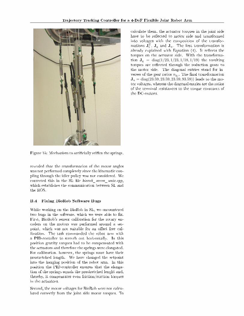
B.3 Veri�cation of Sensor Value Processing

During our work on the robot, we encountered prob-lems with the angle sensors and decided to verify ifthe motor angles are being correctly transformed andgiven out in SL. In order to do that, we decided to arti-�cially make the springs sti� by the mechanism shownin Figures 15 and perform measurements with thequasi rigid robot to eventually re-estimate the trans-formation matrix between the motor and joint sensors.Therefore we designed and built mechanical construc-tions to sti�en the springs. We noticed that the motorangles are being transformed into joint space by theBioRob API, which we had no access to. Our method


Figure 15: Mechanism to arti�cially sti�en the springs.

revealed that the transformation of the motor angleswas not performed completely since the kinematic cou-pling through the idler pulley was not considered. Wecorrected this in the SL �le biorob_servo_unix.cpp,which establishes the communication between SL andthe ROS.

B.4 Fixing BioRob Software Bugs

While working on the BioRob in SL, we encounteredtwo bugs in the software, which we were able to �x.First, BioRob's sensor calibration for the rotary en-coders on the motors was performed around a set-point, which was not suitable for an o�set free cal-ibration. The task commanded the robot arm witha PID-contoller to stretch out horizontally. In thisposition gravity torques had to be compensated withthe actuators and therefore the springs were elongated.For calibration, however, the springs must have theirprestretched length. We have changed the setpointinto the hanging position of the robot arm. In thisposition the PID-controller ensures that the elonga-tion of the springs equals the prestretched lenght and,thereby, it compensates even friction/stiction torquesin the actuators.

Second, the motor voltages for BioRob were not calcu-lated correctly from the joint side motor torques. To

calculate them, the actuator torques in the joint sidehave to be re�ected to motor side and transformedinto voltages with the composition of the transfor-mations JT

t , Jg and Ju. The �rst transformation isalready explained with Equation (4). It re�ects thetorques on the actuator side. With the transforma-tion Jg = diag(1/23, 1/23, 1/18, 1/19) the resultingtorques are re�ected through the reduction gears tothe motor side. The diagonal entries stand for in-verses of the gear ratios ngi . The �nal transformationJu = diag(23.59, 23.59, 23.59, 93.59)) leads to the mo-tor voltages, whereas the diagonal entries are the ratiosof the terminal resistances to the torque constants ofthe DC-motors.

raTjectory racTking Controller for a 4-DoF Flexible … · raTjectory racTking Controller for a...

Documents

Transcript of raTjectory racTking Controller for a 4-DoF Flexible … · raTjectory racTking Controller for a...