A Novel 4-DOF Parallel Manipulator H4 - InTech -...

19

A Novel 4-DOF Parallel Manipulator H4

Jinbo Wu1 and Zhouping Yin2

1 Traffic Science & Engineering College 2State Key Laboratory of Digital Manufacturing Equipment and Technology

Huazhong University of Science & Technology China

1. Introduction

Parallel manipulators have the advantages of high stiffness and low inertia compared to serial mechanisms. Based on the Steward-Gough platform architecture, a lot of 6-DOF mechanical devices have been proposed. The 6-DOF parallel manipulators suffer from a small workspace, complex mechanical design, and difficult motion generation and control due to their complex kinematic analysis. To overcome these shortcomings, the limited-DOF manipulator, which has fewer than 6 DOFs, can be found in many production lines. It is clear today that most attention has been paid to 3-DOF family among the limited-DOF parallel manipulators (Carretero, 2000). However, in many industrial situations, there is a need for equipment providing more than 3-DOFs. For example, for most pick-and-place applications in semiconductor manufacturing, at least 4 DOFs are required (3 translation to move the carried die from one point to the other, 1 rotation to adjust the orientation in its final location). A new family of 4-dof parallel manipulators called H4 that could be useful for high-speed pick-and-place applications is proposed by Pierrot and Company (Pierrot, 1999). The H4 manipulator offers 3 DOFs in translation and 1 DOF in rotation about a given axis. The H4 manipulator is useful for high-speed handling in robotics and milling in machine-tool industry since it is a fully-parallel mechanism with no passive chain and able to provide high performance in terms of speed and acceleration. This chapter discusses the kinematic analysis of the H4 manipulator. In section 2, synthesis methods for designing H4 are presented, and various possible mechanical architectures of the parallel manipulator are exposed. Section 3 discusses the inverse and forward kinematics problem of H4. Section 4 deals with singularity analysis of H4 utilizing line geometry tools and screw theory. Section 5 concludes this chapter by providing the development tendency of the parallel manipulators.

2. Structural synthesis and architectures

2.1 General concept of H4

Parallel manipulators are constituted of a moving platform that is connected to a fixed base by several chains (limbs). Generally, the number of limbs is equal to the degrees of freedom (DOF) of the moving platform such that each limb is driven by no more than one actuator and all actuators can be mounted on or near the fixed base. By acting on the limbs the

Source: Parallel Manipulators, Towards New Applications, Book edited by: Huapeng Wu, ISBN 978-3-902613-40-0, pp. 506, April 2008, I-Tech Education and Publishing, Vienna, Austria

Ope

n A

cces

s D

atab

ase

ww

w.in

tehw

eb.c

om

www.intechopen.com

Parallel Manipulators, Towards New Applications

406

platform pose (position and orientation) is controlled. Moreover, if the actuators are locked, the manipulator will become an isostatic structure in which all the legs carry the external loads applied to the platform. This feature makes the parallel manipulators with high stiffness possible throughout the whole space. From the first ideas proposed by Gough (Gough, 1956) or Steward (Steward, 1965), a lot of interesting mechanical devices or design methods have been extensively studied. In the beginning, many structures were based on the ingenuity of the researchers and not on a systematic approach. Subsequently, a new research domain called structure (or type) synthesis was proposed, in which vaious methodologies were tried to generate all the structures that have a desired kinematic performance. The most widely used synthesis approaches (and their variants) are graph theory, group theory and screw theory (Merlet, 2006). In this section, we will not discuss these theoretical problems, but focus on the structure generation of H4. The 6-DOF parallel manipulators generally suffer from a small workspace, complex mechanical design and difficult motion generation and control due to their complex kinematic anslysis. To overcome these shortcomings, new structures for parallel manipulators having less than 6-DOF (which are called limited-DOF manipulators in this chapter, although many of these new structures were known well before) are explored. There is an overriding motivation behind such efforts: limited-DOF manipulators may be needed for many applications. For example, parallel wrists need only three rotational DOFs. It is clear today that most attention has been paid to 3-DOF family among the limited-DOF parallel manipulators (Gosselin & Angeles, 1989; Agrawal et al., 1995; Gosselin & St-Pierre, 1997; Fattah & Kasaei, 2000; Gregorio, 2001). However, in many industrial situations, there is a need for equipment providing more than 3 DOFs arranged in parallel and based on simpler arrangements than 6-DOF strctures. The reference (Cheung et al., 2002) developed a 4-DOF parallel manipulator E4 which could be used in a semiconductor packaging system. It is in the early 80’s when Reymond Clavel comes up with the brilliant idea of using parallelograms to build a parallel robot with three translational and one rotational degree of freedom (Bonev, 2001). Contrary to opinions published elsewhere, his inspiration was truly original and does not come from any parallel mechanism patents. Professor Clavel called his creation the Delta robot. The new family of 4-DOF parallel manipulators called H4 that could be useful for high-speed pick-and-place applications is just based on the idea of Delta structure (Pierrot & Company, 1999; Company & Pierrot, 1999). The prototype built in the Robotics Department of LIRMM can reach 10g accelerations and velocities higher than 5m/s (Robotics Department of LIRMM).

2.1.1 Delta structure

Even if an incredibly large number of different structures have been proposed by academic researchers in the last 30 years, most of these that are used widely in industry can be classfied into two basic types: the Delta structure and the so-called “hexapod“ with 6 U-P-S chains in parallel (U-P-S: Universal-Prismatic-Spherical). This may be a result of either the exceptional simplicity of the Delta 3-DOF solution, or the enormous research effort dedicated to “hexapod“ (Company, 1999). The basic idea behind the Delta parallel robot design is the use of parallelograms. A parallelogram allows an output link to remain at a fixed orientation with respect to an input link. The use of three such parallelograms restrain completely the orientation of the mobile platform which remains only with three purely translational degrees of freedom. The input

www.intechopen.com


407

links of the three parallelograms are mounted on rotating levers via revolute joints. The revolute joints of the rotating levers are actuated in two different ways: with rotational (DC or AC servo) motors or with linear actuators. Finally, a fouth leg is used to transmit rotary motion from the base to an end-effector mounted on the mobile platform. Fig.1 shows the most famous Delta robot with three translation degrees of freedom, which was initially developed at École Polytechnique from Lausanne by Clavel (Clavel, 1988). All the kinematic chains of this robot are of the RRPaR type: a motor makes a revolute joint rotate about an axis w. On this joint is a lever, at the end of which another joint of the R type is set, with axis parallel to w. A parallelogram Pa is fixed to this joint, and allows translation in the direction parallel to w. At the end of this parallelogram is a joint of the R type, with axis parallel to w, and which is linked to the end effector.

Fig.1. The Delta structure proposed by Prof. Clavel and one of its industrial version, the CE33 (courtesy of SIG Pack Systems)

The Delta robot is firstly marked by the two Swiss brothers Marc-Olivier and Pascal Demaurex who created the Demaurex company (Bonev, 2001). The joint-and-loop graph of the Delta robot and one of its equivalent structures are shown in Fig.2, where P, R and S represent prismatic, revolute and spherical joint respectively. The displacement of the end-effector of the Delta robot is the result of the movement of the three articulated arms mounted on the base, each of which are connected to a pair of parallel rods. The three orientations are eliminated by joining the rods in a common termination and the three parallelograms ensure the stability of the end-effector. It is noted that the rotary actuator and lever part of the Delta could be replaced by a linear actuator, as suggested by Clavel itself and Zobel (Zobel, 1996). This type of Delta is sometime called a Linapod or a linear Delta.

www.intechopen.com


408

P/R R

R

R

R

RR

P/R R

R

R

R

RR

P/R R

R

R

R

RR

Base End-effector

actuated “arm“ parallelogram

P/R

S

S

S

S

P/R

S

S

S

S

P/R

S

S

S

S

Fig.2. Joint-and-loop graph of the Delta robot and one of its equivalent structure

2.1.2 Structure derivation of H4

H4 is based on 4 independent kinematic chains between the base and the nacelle, each chain is actuated where each actuator is fixed on the base (Pierrot & Company, 1999; Company & Pierrot, 1999). Such technological and conceptual ideas have already proven their efficiency on high-speed equipment for the Delta robot. So, knowing the advantages of this family of mechanisms, it is interesting to recall a few important design features of the Delta robot. The Delta robot is based on three actuated linear or rotational joints, and three pairs of rods equipped with ball joints at each end. As a matter of fact, two ball joints on each rod introduce an internal DOF for the rod which can rotate about its own axis. An arrangement such as the one depicted in Fig.3 suppresses these internal DOF and keeps the same global behaviour. To go a little further, it is possible to consider each pair of rods (that is: two U-S chains parallel one to the other) as equivalent to a unique rod equipped with universal joints at each extremity. The admissible motions for both chains are not exactly the same, but they can be regarded as “equivalent” in terms of number and type of degrees of motion.

P/R

U

U

S

S

P/R

U

U

S

S

P/R

U

U

S

S Fig.3. The structure of a Delta robot with no internal DOF

www.intechopen.com


409

In order to define the basic principle of a 4-DOF mechanism, the classical kinematics formulas can be used. For a mechanism with a “closed loop” (a chain going from ground to the nacelle, and then back to ground), its mobility is given by:

LdofmlN

i

i 61

−=∑= (1)

where L is the number of loops; idof is the number of DOF of the ith link;

lN is the number

of links. For a fully-parallel 4-DOF mechanisms involving no passive chain, 3=L and 4=m . Thus:

( ) 223641

=×+=∑=lN

i

idof

The four P-U-U chains provide: dof2054 =× . Thus each additional joint must be only 1

DOF joint. Two rotational joints can be used because such joints are extremely easy to manufacture with good accuracy at low cost. So the arrangement shown in Fig.3 are created, each pair is connected to the nacelle by an R joint. Note that the actuated prismatic joints can be replaced by actuated rotational joints, and that the U-U chains can be replaced by (U-S)2 chains as well (shown in Fig.3(b)). To date, the conditions for a 4-DOF machine have been set up. The conditions to be fulfilled for obtaining 3 translations and 1 rotation about a given axis should be provided.

P/R U

U

U

U

P/R

U

U

U

U

P/R

U

U

S

S

P/R

U

U

S

S

P/R

U

U

S

S

R

R

P/R

P/R

P/R

U

U

S

S

R

R

(a) (b) Fig.4. Architecture scheme of H4

The demonstration of “quasi-equivalence” between P-U-U and P-(U-S)2 is proposed in (Company et al., 2003). The following discusses the possible motion of H4 (Pierrot & Company, 1999; Company & Pierrot, 1999). Firstly, assume that the two rods of the (U-S)2 chains are parallel to each other. Fig.5 shows a simple scheme of a possible H4 structure. Ai and Bi are the centers of segments Ai1Ai2 and

www.intechopen.com


410

Bi1Bi2, respectively. Note Ai1Bi1=Ai2Bi2=AiBi and ui=Bi1Bi2. With such notations, the impossible motion for the tip of each P-(U-S)2 chain is the rotation about: AiBi×ui.

B12

C2

B1

A12

A11

A1

v

C1

A21 A22

A41

A42

B11 Fig.5 A simple scheme of H4 structure

The link B1B2 is connected to the ground by P-(U-S)2 chains. Each chain provides 3 translations; thus the link B1B2 can undergo the same translations. Moreover B1B2 cannot rotate about A1B1×u1, neither about A2B2×u2 (because the motion that B1B2 cannot make is the sum of the impossible motions for each chain). Consequently, B1B2 can only rotate about the vector normal to the two previous vectors, namely:

( ) ( )222111 uBAuBA ××× (2)

The link B3B4 has 3 DOFs in translation, and can only rotates about:

( ) ( )444333 uBAuBA ××× (3)

The link C1C2 is connected, on one side, to B1B2 by a revolute joint whose direction is represented by vector v1, on the other side, to B3B4 by a revolute joint whose direction is represented by vector v2. Thus, on each side of the nacelle, there are two “meta-chains” which have 5 DOFs. The first chain has 3 translations and 2 rotations about v1 and ( ) ( )222111 uBAuBA ××× respectively. The rotation about ( ) ( ) 1222111 vuBAuBA ×××× is

impossible. The second “mecha-chain” has 3 translations and 2 rotations about v2 and ( ) ( )444333 uBAuBA ××× respectively. The rotation about ( ) ( ) 2444333 vuBAuBA ×××× is

impossible. So the possible motions of the nacelle are 3 translations and 1 rotation about ( ) ( )[ ] ( ) ( )[ ]24443331222111 vuBAuBAvuBAuBA ××××××××× . When the two revolute joints

www.intechopen.com


411

placed on the nacelle have the same direction represented by a unit vector v, the existence of a rotational motion about v can be written as follows:

( )[ ] ( )[ ] vvwwvww ααα =×××××≠∃ 43210, (4)

Where iiii uBAw ×= . Equation (4) is equivalent to:

( )[ ] ( )[ ]{ } vvvvwwvww ⋅=⋅××××× α4321

Since v is a unit vector, then we can obtain

( )[ ] ( )[ ]{ } 04321 ≠=××××× αvwwvww

Thus:

( ) ( )[ ] ( ) ( )[ ] 043212143 ≠=⋅×××−=××⋅× αvwwwwvwwww

So, the necessary condition that the nacelle can rotate about a given axis is:

( ) ( )[ ] 04321 ≠⋅××× vwwww (5)

It should be noted that the previous condition is only a necessary condition and any singular configuration is not taken into account. The following should demonstrate that the two rods of the P-(U-S)2 chain are parallel to each other when the nacelle moves, so the necessary condition (7) is also satisfied. The rods of the P-(U-S)2 chain will stay parallel to each other if both links B1B2 and B3B4 move only in translation with respect to the ground. As a matter of fact, the possible motions of the nacelle imply that the two pivots fixed on the nacelle along the direction of vector v will keep this direction. Thus the only possible rotation for B1B2 and B3B4 is about vector v. But equation (2) indicates that B1B2 can only rotate about

21 ww × . So, as long as

21 ww × and v are not collinear, the link B1B2 has no possible rotation. A similar remark can

be made for B3B4, leading to the two following conditions:

vww

vww

≠×≠×

43

21 (6)

In conclusion, if conditions (6) are fulfilled, the links B1B2 and B3B4 move only in translation, and the rods in a pair will stay parallel to each other.

2.1.3 H4 mechanism with symmetrical design

In this chapter, the symmetrical design of H4 refers to the structure scheme based on four identical P-U-U chains or P-(U-S)2 chains. The four identical chains provide 4×5=20 DOFs. Thus, two additional 1-DOF joints are needed. H4 uses two rotational joints because they are easy to manufacture with good accuracy at low cost. Two types of typical architecture scheme of H4 are shown in Fig.4. Note that the U-U chains can be replaced by (U-S)2 chains. Moreover, the actuated prismatic joints could be replaced by actuated rotational joints as well. A symmetrical mechanism with prismatic actuators is show in Fig.6 (a), while an equivalent mechanism with rotational actuators is shown in Fig.6 (b).

www.intechopen.com


412

(a) (b)

Fig.6. Symmetrical H4 with actuated prismatic joints and rotational joints

2.1.3 H4 mechanism with asymmetrical design

The link B1B2 has three translations and a possible rotation about a vector given by equation (2). It is possible to create more advanced mechanisms based on a particular case of equation (2). For example, if u1=u2, then equation (2) becomes:

( ) ( ) 1122111 uuBAuBA β=×××

As long as 2211 BABA ≠ , then 0≠β . So the only possible rotation of this link is about vector

u1. Thus, the first “meta-chain” already fulfilled our requirements: 3 translations and 1 rotation about a given axis. However, this “meta-chain” is only equipped with 2 actuators; thus 2 other chains (with one actuator each) are needed in parallel to lead to a fully-parallel manipulator. If the first “meta-chain” is constituted of two P-U-U chains, it provides 2×5=10 DOFs. So the two additional chains that constitute the second “meta-chain” should be 6

P/R U

U

U

U

P/R

U

U

S

S

P/R

U

U

S

S

P/R

U

U

S

S

P/R U S

P/R

P/R

P/R U S

(a) (b) Fig.7 Asymmetrical design of H4

www.intechopen.com


413

DOFs, which are obviously compatible with the motions offered by the first “meta-chain”. Such mechanical structures are named asymmetrical H4 (Pierrot & Company, 1999; Company & Pierrot, 1999). An asymmetrical design of H4 using two P-U-Us and two P-U-S’s is shown in Fig.7 (a). The P-U-U’s can be replaced by P-(U-S)2’s, as shown in Fig.7 (b).

2.2 Evolution of H4

A new trend in the researches on parallel robotics is the development of lower mobility manipulators. Indeed, a lot of applications do not need six DOFs. A classification proposed by Brogardh (Brogardh, 2002) gives the necessary number of DOF for different industrial applications. He shows that applications such as pick-and-place, assembly, cutting, measurement, etc. just need from three up to five DOFs. The parallel manipulator H4 can provide three translations and one rotation about a fixed

axis, which are also called Schonflies motions (Hervé, 1999). SCARA robots were the first manipulators developed to produce these movements. Due their serial architecture, these robots involve high moving masses which are not suitable for high dynamics. Parallel architecture can overcome this problem. Delta robot is first introduced by Clavel to execute Schonflies motions (Clavel, 1988). This architecture is able to produce three translations and one rotational motion is obtained using a central “telescopic” leg built with universal and prismatic joints. This RUPUR chain suffers from a short service life, and involves a bad stiffness of the rotation motion. Orthoglide (Chablat, 2002) is another parallel robot that can provide Schonflies motions using linear actuators. Its particularity is to be isotropic at the center of its workspace. The machine tool HITA STT has been proposed to produce Schonflies motions (Thurneysen et al, 2002). The particularity of this architecture is to use additional parts in the traveling plate in order to amplify the rotational motion. Other Schonflies motion generators include Gross Manipulator (Angeles et al., 2000), SMG (Angeles, 2005), Kanuk and Manta (Rolland et al., 1999) robots. In order to avoid the central telescopic leg of the Delta robot, in 1999, the Montpellier Laboratory of Computer Science, Robotics, and Microelectronics (LIRMM) in French invented the parallel manipulator H4 which used the concept of articulated traveling plate. The rotational movement is obtained using an internal mobility on the traveling plate, and a transforming device gives the desired range of rotational motion. Because placing actuators in a symmetrical way (i.e. at 90° one relatively to each other) involves “internal singularities” (Pierrot & Company, 1999), the robot has to be built using a particular arrangement of motors. This non-symmetrical arrangement entails a non-homogeneous behavior in the workspace and a limited stiffness of the robot (Company et al., 2005). Later, based on the concept of H4, an improved mechanical structure called I4 is proposed by LIRMM (Krut et al., 2004; Krut et al., 2003). The internal mobility of I4 is obtained with a prismatic joint (Fig. 8). The advantage of this architecture is to authorize a symmetrical arrangement of the actuators. As demonstrates by Krut (Krut et al., 2004), it is possible to place the actuators at 90° one relatively to each other. However, this architecture is more adapted to machine-tool application than to high speed pick-and-place. Indeed, commercial prismatic joints are not suitable for high speed and high accelerations, and have a short service life under such conditions. This inconvenient is due to the high pressure exerted on the balls of these elements at high acceleration conditions. Based on H4 and I4 architecture, an evolution of these mechanisms, named Part 4, has been developed with the wish of reaching high speeds

www.intechopen.com


414

and accelerations (Nabat et al., 2005). A paper written by Nabat (Nabat et al., 2006) presented experimental results showing that Part 4 was able to reach an acceleration of 15G. Part 4 is a parallel manipulator composed of four closed kinematic chains and an articulated traveling plate. The kinematic chains are similar for Delta, H4 and I4, each of which is composed of an arm and a spatial parallelogram (forearm) linked with spherical joints. The traveling plate is composed of four parts: two main parts (1, 2) linked by two bars (3, 4) with revolute joints (see Fig.9). Thus, its shape is a planar parallelogram and the internal mobility of this traveling plate is a circular translation. Generally, the “natural “range of the rotational operational motion is small, in order to make a complete turn: [-π; π], an amplification system has to be added on the traveling plate. Several options are available for this amplification such as gears or belt/pulleys. The prototype shown in Fig.9 (b) has been built using belt/pulleys system, with the first pulley fixed on one half traveling plate, and the second one is linked with a revolute joint to the second half traveling plate. Due to its traveling plate having the shape of a planar parallelogram, Part 4 has all the advantages of the previous robots, without their drawbacks. The traveling plate of this robot is articulated and is exclusively realized with revolute joints. Nabat (Nabat et al., 2006) has demonstrated that it is possible to have the same arrangements of the actuators as I4. Thus, this robot is well suited to reach high dynamics and, at the same time, to have a good stiffness and a homogenous behavior in the workspace.

(a) Overview of I4 prototype (b) Articulated traveling plate

Fig.8. I4 prototype (courtesy of LIRMM)

The use of base-mounted actuators and low-mass links allows the traveling plate to achieve great accelerations. This makes this type of parallel manipulator a perfect candidate for pick and place operations of light objects. Especially for semiconductor end-package equipments, which need high-speed and high-precision pick-and-place movement, these parallel manipulators provide a novel solution scheme. In this chapter, only H4 is considered, because it firstly provides the most important concept of traveling plate. Based on the analytical method of H4, other types of evolution structure can be analyzed conveniently.

www.intechopen.com


415

(b) Articulated traveling plate (a) Overview of Part4 prototype Fig.9. Part4 prototype (courtesy of LIRMM)

3. Kinematic analysis

This section will examine the relations between the actuated joint coordinates of H4 and the nacelle (or traveling plate) pose.

3.1 Inverse kinematics

The relation giving the actuated joint coordinates for a given pose of the end-effector is called the inverse kinematics, which is simple for parallel robots. The inverse kinematics consists in establishing the value of the joint coordinates corresponding to the end-effector configuration. Establishing the inverse kinematics is essential for the position control of parallel robots. There are multiple ways to represent the pose of a rigid body through a set of parameters X. The most classical way is to use the coordinates in a reference frame of a given point C of the body, and three angles to represent its orientation. But there are other ways such as kinematic mapping which maps the displacement to a 6-dimensional hyperquadric, the Study quadric, in a seventh-dimensional projective space. The kinematic mapping may have an interest as equations involving displacement are algebraic (and the structure of algebraic varieties is better understood than other non-linear structures) and may have interesting properties, for example, stating that a point submitted to a displacement has to lie on a given sphere is easily written as a quadric equation using Study coordinates (Merlet, 2006).

3.1.1 Analytic method

For a fully-parallel mechanism, each of the chains link the base to the moving platform. If A represents the end of the chain that is linked to the base, and B the end of the chain that is linked to the moving platform. By construction the coordinates of A are known in a fixed reference frame, while the coordinates of B may be determined from the moving platform position and orientation. Hence the vector AB is fundamental data for the inverse kinematic problem, this is why it plays a crucial role in the solution. In order to write the position relationship of H4, consider the robotic structure (see Fig.10, chain #4 is not plotted for sake of simplicity). The geometrical parameters of the manipulator at hand are defined as follows:

www.intechopen.com


416

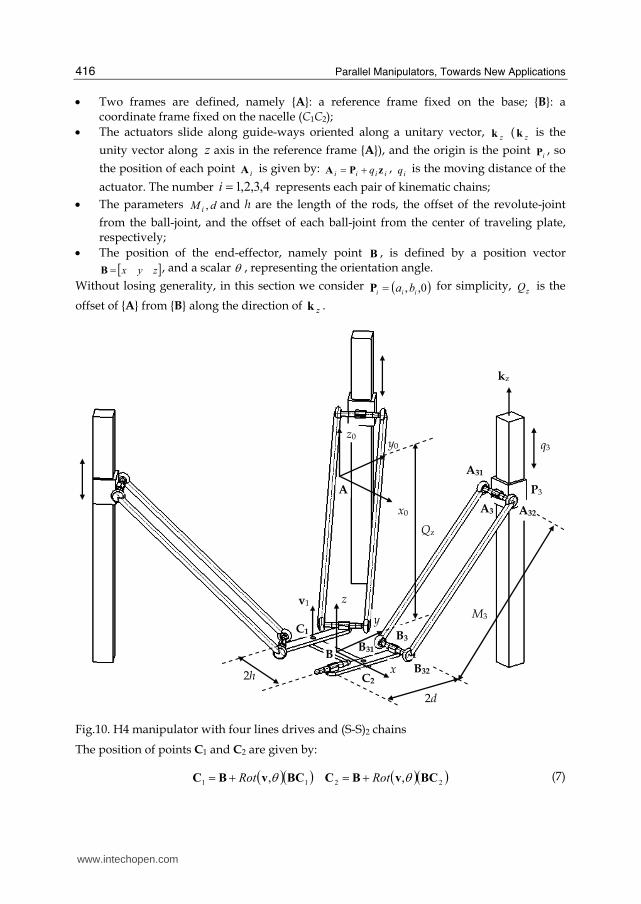
• Two frames are defined, namely {A}: a reference frame fixed on the base; {B}: a coordinate frame fixed on the nacelle (C1C2); • The actuators slide along guide-ways oriented along a unitary vector,

zk (zk is the

unity vector along z axis in the reference frame {A}), and the origin is the point iP , so

the position of each point iA is given by:

iiii q zPA += , iq is the moving distance of the

actuator. The number 4,3,2,1=i represents each pair of kinematic chains; • The parameters dM i , and h are the length of the rods, the offset of the revolute-joint

from the ball-joint, and the offset of each ball-joint from the center of traveling plate, respectively;

• The position of the end-effector, namely point B , is defined by a position vector [ ]zyx=B , and a scalar θ , representing the orientation angle.

Without losing generality, in this section we consider ( )0,, iii ba=P for simplicity, zQ is the

offset of {A} from {B} along the direction of zk .

x0

y0z0

A

v1

C1

B

x

y

z

C2

Qz

A31

A3

B3

B31

M3

A32

B32

2d

2h

P3

q3

kz

Fig.10. H4 manipulator with four lines drives and (S-S)2 chains

The position of points C1 and C2 are given by:

( )( ) ( )( )2211 ,, BCvBCBCvBC θθ RotRot +=+= (7)

www.intechopen.com


417

Where ( )θ,vRot denotes the rotation matrix of nacelle with respect to reference frame. The

position of each point Bi is given by:

42243223

21121111

BCCBBCCB

BCCBBCCB

+=+=+=+= (8)

The position relationship can then be written as:

22

iii M=BA (9)

Then for the first axis:

( )( )[ ] 11111111 , zPBCBCvBBA qRot −−++= θ

( ) 2

1111

2

1

2

11 2 dzdBA +⋅−= qq (10)

where ( )( ) 11111 , PBCBCvBd −++= θRot . Finally, the two solutions are given by:

( ) 2

1

2

1

2

11111 dzdzd −+⋅±⋅= Mq (11)

Similar derivations give the solution for q2, q3 and q4.

3.1.2 Geometrical method

The geometrical approach to the inverse kinematics problem is to consider that the extremities A, B of each chain have a known position in 3D space. The leg can be cut at a point M and two different mechanisms MA, MB constituted of the chain between A, M and the chain between B, M can be gotten. The free motion of the joints in these two chains will be such that point M, considered as a member of MA, will lie on a variety VA, while considered as a member of MB it will lie on a variety VB. If assume the mechanism have only classical lower pairs, these varieties will be algebraic with dimensions dA, dB. In the 3D space, a variety of dimension d is defined through a set of 3-d independent equations, and hence VA, VB will be defined by 3-dA and 3-dB equations. The solutions of the inverse kinematic problem lie at the intersection of these varieties. As the number of of solutions must be finite (otherwise the robot cannot be controlled), the rank of the intersection variety must be 0. In other words, in order to determine the 3 coordinates of the points, 3-dA+3-dB should equal to 3 or dA+dB equal to 3 (Merlet, 2006). The key problem about the geometrical mthod rests with the choice of the cutting point. For the H4 structure shown in Fig.10, Bi are chosen as the cutting points. Points Bi has to lie on a sphere centered at Ai with radius Mi, while for the nacelle, the coordinates of Points Bi can be described as (8). Hence to obtain the intersection of these 2 varieties the known distance between A, B of should be equal to Mi: this equation will give the joint coordinates qi. The same results can be obtained as described as (11).

3.2 Direct kinematics Direct kinematics addresses the problem of determining the pose of the end-effector of a parallel manipulator from its actuated joint coordinates. This relation has a clear practical interest for the control of the pose of the manipulator, but also for the velocity control of the end-effector.

www.intechopen.com


418

In general, the solutions for determining the pose of the end-effector from measurements of the minimal set of joint coordinates that are necessary for control purposes is not unique. There are several ways of assembling a parallel manipulator with given actuated joint coordinates, and generally the direct kinematic relationship cannot be expressed in an analytical manner. Although various methods have been presented for finding all the solutions for this problem and their computation times are decreasing (Faugère, 1995; Hesselbach & Kerle, 1995; Gosselin, 1996; Merlet, 2004), it is still difficult to use these algorithms in a real time context. Furthermore, there is no known algorithm that allows the determination of the current pose of the platform among the set of solutions. The numerical methods using a-priori information on the current pose are more compatible with a real-time context, while their convergence and robustness is an important issue. As direct kinematics is an important issue for control, it may be necessary and interesting to investigate how to improve the computation time. Besides the progress in algorithms and processor speed, one possible approach to solve these problem is to add sensors (i.e. to have more than n sensors for a n-DOF manipulator) to obtain information, allowing a faster calculation of the current pose of the platform, at the cost of more complex hardware (Bonev et al., 2001; Chui & Perng; 2001; Parenti-Castelli, 2001). Merlet has pointed out several unsolved problems about the parallel robot’s direct kinematics (Merlet, 2000). Especially the algebraic geometry and computational kinematics should bring about enough attention. The first step of solving direct kinematics is to determine a bound on its maximal number of solution. Then, the equations are reduced for the system to obtain the solution of a univariate polynomial whose degree should be determined in the previous analysis. Many researchers have tried to obtained closed-form solutions of parallel robots in a univariate polynomial equation. Especially, the 3- and 6- DOFs parallel robots, e.g., planar, Delta, Steward platform and Hexapod robots, have been mainly considered. This section provides a univariate polynomial equation for H4. It is shown that the solutions of the forward kinematics yield a 16th degree polynomial in a single variable (Choi et al., 2003).

3.2.1 Forward kinematics formulation

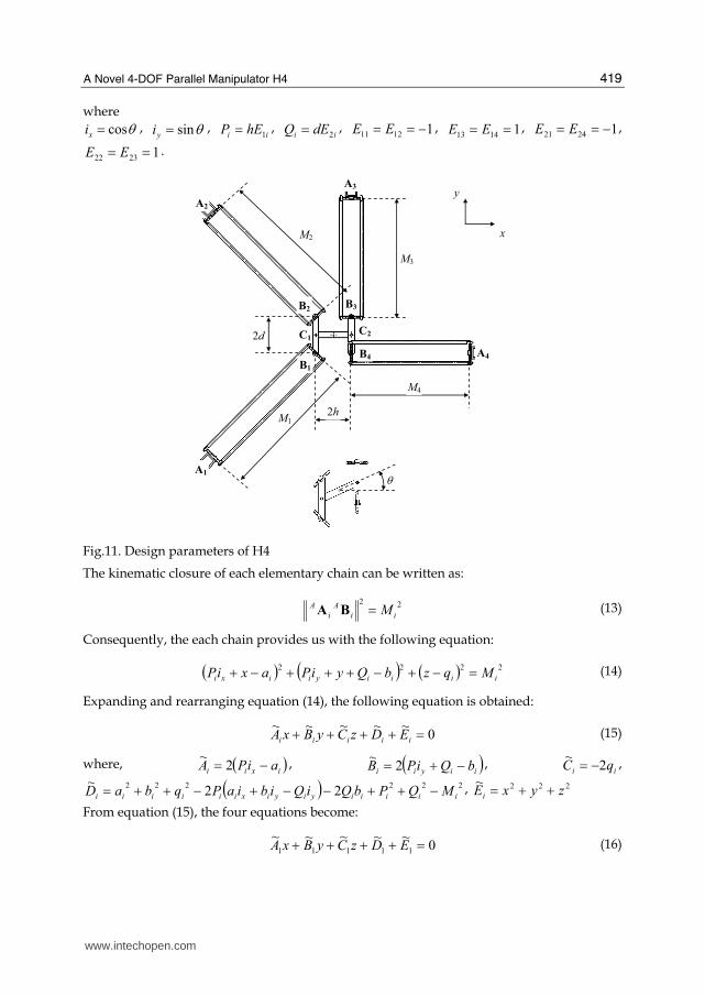
The forward kinematics of the H4 is the problem of computing the position and orientation of the nacelle (traveling plate) form the motor angles or the moving distance of the actuator. To get a closed-form solution, a univariate polynomial equation needs to be solved. The following method is extracted from the paper written by Choi (Choi et al., 2003). The kinematic structure of H4 is shown in Fig.10 and design parameters are shown in Fig.11. The nacelle is composed of three parts (two lateral bars and one central bar). The four points B1, B2, B3 and B4 form a parallelogram. Let

i

AB and i

A A represent the homogeneous

coordinates of the points Bi in {A} and Ai in {A} respectively. Then the homogeneous coordinates of

i

AB and i

A A can be written as:

[ ]Tiiii

A

iyi

xi

ii

i

i

A

qbaA

z

QyiP

xiP

z

dEhEy

hEx

B

1

11

sin

cos

21

1

=⎥⎥⎥⎥

⎦

⎤

⎢⎢⎢⎢

⎣

⎡+++

=⎥⎥⎥⎥

⎦

⎤

⎢⎢⎢⎢

⎣

⎡++

+= θ

θ (12)

www.intechopen.com


419

where θcos=xi , θsin=yi , ii hEP 1= ,

ii dEQ 2= , 11211 −== EE , 11413 == EE , 12421 −== EE ,

12322 == EE .

A1

B1

A2

B2

A3

B3

B4 A4

2d

2hM1

M2

M3

M4

C1C2

x

y

θ

Fig.11. Design parameters of H4

The kinematic closure of each elementary chain can be written as:

22

ii

A

i

A M=BA (13)

Consequently, the each chain provides us with the following equation:

( ) ( ) ( ) 2222

iiiiyiixi MqzbQyiPaxiP =−+−+++−+ (14)

Expanding and rearranging equation (14), the following equation is obtained:

0~~~~~ =++++ iiiii EDzCyBxA (15)

where, ( )ixii aiPA −= 2~ , ( )iiyii bQiPB −+= 2

~ , ii qC 2

~ −= , ( ) 22222222

~iiiiiyiyixiiiiii MQPbQiQibiaPqbaD −++−−+−++= , 222~

zyxEi ++=

From equation (15), the four equations become:

0~~~~~

11111 =++++ EDzCyBxA (16)

www.intechopen.com


420

0~~~~~

22222 =++++ EDzCyBxA (17)

0~~~~~

33333 =++++ EDzCyBxA (18)

0~~~~~

44444 =++++ EDzCyBxA (19)

Choosing any three from the above four equations, we can eliminate x2, y2 and z2 simultaneously and obtain an equation with variables x, y and z. Subtracting equation (18) from equation (17) and equation (19) from equation (17) respectively, the following two equations are obtained, which are used to eliminate x and y to obtain a polynomial in a single variable z.

023232323 =Δ+Δ+Δ+Δ DzCyBxA (20)

024242424 =Δ+Δ+Δ+Δ DzCyBxA (21)

where, ( )3223

~~AAA −=Δ , ( )3223

~~BBB −=Δ , ( )3223

~~CCC −=Δ , ( )3223

~~DDD −=Δ , ( )4224

~~AAA −=Δ , ( )

4224

~~BBB −=Δ , ( )4224

~~CCC −=Δ , ( )4224

~~DDD −=Δ .

From equation (20) and (21), x and y are solved as:

21

0

1211 ezez

x +=ΔΔ+Δ= (22)

43

0

2221 ezez

y +=ΔΔ+Δ= (23)

where, 0

111 Δ

Δ=e , 0

122 Δ

Δ=e , 0

213 Δ

Δ=e , 0

224 Δ

Δ=e , with 232424230 BABA ΔΔ−ΔΔ=Δ ,

2324242311 CBCB ΔΔ−ΔΔ=Δ , 2324242312 DBDB ΔΔ−ΔΔ=Δ ,

2423232421 CACA ΔΔ−ΔΔ=Δ ,

2423232422 DADA ΔΔ−ΔΔ=Δ .

Substituting equations (22) and (23) into equation (17), the following quadratic equation is obtained:

021

2

0 =++ λλλ zz (24)

where, 12

3

2

10 ++= eeλ , 2321243211

~~~22 CeBeAeeee ++++=λ ,

24222

2

4

2

22

~~~DeBeAee ++++=λ .

From equation (24), z can be calculated as:

0

1

2λρλ +−=z (25)

where,

20

2

1 4 λλλρ −±= (26)

www.intechopen.com


421

Substituting equations (22), (23) and (25) into equation (16), the following equation is obtained:

( ) 0422 2011

2

111

2 =′+′−+′−− λλλλλρλλρ (27)

where, 1311143211

~~~22 CeBeAeeee ++++=′λ ,

14121

2

4

2

22

~~~DeBeAee ++++=′λ .

The variable ρ can be calculated from equation (27):

( ) 20

2

111 4 λλλλλρ ′−′±′−= (28)

So the right parts of equations (26) and (28) are equivalent:

( ) 20

2

120

2

111 44 λλλλλλλλ −±=′−′±′− (29)

By taking the second power of the both sides of equation (29), a polynomial equation with variables

xi and yi can be obtained as follows:

( )[ ] 02

20212110 =Δ⋅+′−′⋅Δ λλλλλλλλ (30)

where, 111 λλλ ′−=Δ ,

222 λλλ ′−=Δ . Equation (20) can be rewritten as (Choi et al., 2003):

( ,,,,,,,,,,,,,,,,,,,,,, 53433323334434244435255526667778

yxyxyxyxyxxyxyxyxyxxyxyxyxxyxyxxyxyxxx iiiiiiiiiiiiiiiiiiiiiiiiiiiiiiiiiiiiiif

) 0,,,,,,,,,,,,,,,,,, 40302000065432625242322222 =yxyxyxyxyxyxyxyxyxyxyxxyxyxyxyxyxyxx iiiiiiiiiiiiiiiiiiiiiiiiiiiiiiiiiiii (31)

where ( )nxxxf A,, 21 represents a linear combination of

nxxx A,, 21. The coefficients of

equation (30) are all constant quantities which depend on the geometric parameters of the H4 robot. Using the following well-known trigonometric function:

2

2

1

1

T

Tix +

−= , 21

2

T

Tix += (32)

where ( )2tan θ=T , then equation (31) becomes a polynomial equation in a single variable T

which contains terms up to the 16th power. This means that the mechanism may have up to 16 different configurations for a given set of actuator’s position. Substituting equation (32) into equations (26), (22), (23) and (25), the values of yx,,ρ and z can be gotten respectively.

3.2.2 Numerical example

In this section, a numerical example for the H4 robot shown in Fig.10 and Fig.11 is presented to illustrate the application of the method proposed in the previous section. The design parameters of H4 is chosen as: h=d=6, Qz=42, v=[0 0 1]T, M1=M2= 3 Qz, M3=M4= 2 Qz, the origin coordinates of points Ai and Bi are set as following:

[ ]048481 −−=A , [ ]42661 −−−=B , [ ]048482 −=A , [ ]42662 −−=B ,

www.intechopen.com


422

[ ]04863 =A , [ ]42663 −=B , [ ]06484 −=A , [ ]42664 −−=B ,

[ ]⎥⎥⎥⎦

⎤⎢⎢⎢⎣

⎡−

−==

0000

1011

0111

4321 uuuuu, where

21 iii BBu = .

When the position and orientation of the nacelle are set x=5, y=-5, z=-30, θ=π/6(rad), four actuators’ position which is calculated by inverse kinematics are given by:

q1=13.021, q2=-7.488, q3=9.679, q4=15.770 (33)

For the actuators’ position given by equation (33), Matlab Symbolic Math Toolbox is used to solve the polynomial equation with variable T. The results indicate that there are only twelve solutions, the author believes that there are several repeated roots. This result needs further study. The two real roots are T=0.268 and T=-2.882 respectively. When set T=0.268, the configuration of the nacelle is calculated as: x=5mm, y=-5mm, z=-30mm, θ=0.524(rad), which is the expected solutions. When set T=-2.882, the configuration of the nacelle is calculated as: x=3mm, y=-7.95mm, z=-14.58mm, θ=-2.47(rad). This configuration cannot be realized in practice because of the mutual interference of the parallelograms as shown in Fig.11.

3.3 Jacobian matrix Jacobian matrix relates the actuated joint velocities to the end-effector cartesian velocities, and is essential for the velocity and trajectory control of parallel robots. For parallel manipulators, their inverse Jacobian matrix can be established without a very high complexity, but their Jacobian matrix cannot be obtained directly, even with the help of symbolic computation, except in some particular cases (Bruyninckx, 1997; Pennock & Kassner, 1990). Theoretical analytic formulations of jacobians have been proposed, but require complicated matrix inversions (Dutré et al., 1997; Kim et al., 2000). Generally, the difficulty of the inversion does not lie in the complexity of the algorithm but in the sheer size of the result (Merlet, 2006). The velocity of the nacelle can be defined by resorting to a velocity for the translation, [ ]zyxB

$$$=v and a scalar for the rotation about v, θ$ . Thus, the velocity of points C1 and C2 can be written as follows (Pierrot & Company, 1999):

11Cvvv BBC ×+= θ$

22Cvvv BBC ×+= θ$

Moreover, since the links B1B2 and B3B4 move only in translation, the following relations hold:

121 CBB vvv == 243 CBB vvv ==

On the other hand, velocity of points Ai is given by:

iiA qi

zv $=

where zi is the unit vector along the direction of prismatic. The velocity relationship can then be written thanks to the classical property:

www.intechopen.com


423

iiBiiA ii

BAvBAv ⋅=⋅ (34)

Equation (34) can be written for i=1,…,4 and the results grouped in a matrix form, such as:

xJqJ $$xq =

where

( ) ( ) ( ) ( )⎥⎥⎥⎥

⎦

⎤

⎢⎢⎢⎢

⎣

⎡

⋅⋅

⋅⋅

=444

333

222

111

000

000

000

000

zBA

zBA

zBA

zBA

J q

[ ]Tqqqq 4321$$$$$ =q

( ) ( ) ( ) ( )( ) ( ) ( ) ( )( ) ( ) ( ) ( )( ) ( ) ( ) ( ) ⎥⎥⎥⎥⎥

⎦

⎤

⎢⎢⎢⎢⎢

⎣

⎡

⋅×⋅×⋅×⋅×

=vBCBABABABA

vBCBABABABA

vBCBABABABA

vBCBABABABA

J

244444444

233333333

122222222

111111111

zyx

zyx

zyx

zyx

x

[ ]θ$$$$$ zyx=x

If the mechanism is not in a singular configuration, the inverse Jacobian matrix is described as:

xq JJJ

11 −− = (35)

And the Jacobian matrix is:

qx JJJ

1−= (36)

When the determinant of inverse Jacobian matrix equals to zero, the parallel manipulator is in a singular configuration, which is a general method for identifying the singular configurations of parallel manipulators. But for a manipulator with n<6DOF, it should be noted that it may not be efficient to identify all the singular configurations by determining only the n×n inverse kinematic Jacobian that relates the actuated joint velocities to the possible DOF velocities. Next section will discuss an inverse kinematic Jacobian that involves actuated joints velocities and the full twist of the end-effector, which may be essential for singularity analysis. This type of matrix is coined as overall jacobian by Joshi (Joshi & Tsai, 2002), while Merlet called it a full inverse kinematic jacobian (Merlet, 2006).

3.4 Determination of the joint velocities and twist

The purpose of this section is to calculate the actuated joint (or end-effector) velocities, being given the end-effector (or actuated joint) velocities. In the previous section, equation (35) can be applied to compute the actuated joint velocities directly. For example, the structure and design parameters of H4 is described in Fig.10 and

www.intechopen.com


424

Fig.11, where the following parameters are chosen as described in section 3.2.2. So, according to equation (35), the inverse Jacobian matrix can be expressed as:

⎥⎥⎥⎥

⎦

⎤

⎢⎢⎢⎢

⎣

⎡−

−−−−

=−

0101

6110

6111

6111

1J

This inverse Jacobian matrix can be used to calculate the actuated joint velocity directly when the pose of the nacelle is shown in Fig.11. It is usually difficult, even for robots with less than 6-DOFs robots, to invert J-1 analytically. So a numerical procedure will be needed to calculate the twist of the nacelle from the joint velocities. For a given pose of the end-effector, there are two methods to determine the Jacobian matrix, namely, a numerical inversion algorithm and the quasi-Newton scheme (Reboulet, 1985; Merlet, 2006).

( )kkk JJqJJJ 1

01

−+ −+= $ (37)

where q$ is the actuated joint velocity; J0 denotes the kinematic jacobian matrix calculated

for a given pose. The algorithm stops when the differences between the joint velocities and those that are calculated from the twist are lower than a fixed threshold. For the H4 structure and design parameters described above, when the actuated joint velocities is [ ] [ ]11114321 −== qqqqq , the speed of the nacelle can reach [ ] [ ]125.05.025.05.0 −−== θ$$$$$ zyxx .

3.5 Accelerations analysis This section will determine what are the relations between the actuated joint accelerations and the cartesian and angular accelerations of the end-effector. H4 presents excellent characteristics as to acceleration which can reach 10g. For parallel robots it is generally easy to obtain these relations directly. From the equation xJq $$ 1−= , the following can be obtained by differentiation

xJxJq $$$$$$ 11 −− += (38)

For the various categories of parallel manipulators, the determination of the acceleration equations thus amounts to the determination of the derivative of the inverse kinematic jacobian matrix (Merlet, 2006). But for H4, the method described above is not intuitionistic. So we derive the relations between the actuated joint accelerations and the accelerations of the end-effector using geometric method. From equation (12), accelerations of the point Bi and Ai in {A} can be obtained as:

[ ][ ]TiA

T

iiB

qa

zhEyhExa

i

i

$$$$$$$$$$$$

00

sincos 11

=⋅−⋅−= θθθθ (39)

The acceleration projection of points Bi and Ai on the line AiBi is equal. So the following equation comes into existence:

www.intechopen.com


425

iiBiiA ii

aa BABA ⋅=⋅ (40)

Equation (40) can be written for i=1,…,4 and the results grouped in a matrix form, such as:

xJqJ $$$$aq = (41)

where

[ ]Tqqqq 4321$$$$$$$$$$ =q

( ) ( ) ( ) ( ) ( )( )( ) ( ) ( ) ( ) ( )( )( ) ( ) ( ) ( ) ( )( )( ) ( ) ( ) ( ) ( )( ) ⎥⎥⎥⎥⎥

⎦

⎤

⎢⎢⎢⎢⎢

⎣

⎡

⋅+−⋅+−⋅+−⋅+−

=144444444444

133333333333

122222222222

111111111111

sincos

sincos

sincos

sincos

hE

hE

hE

hE

yxzyx

yxzyx

yxzyx

yxzyx

a

θθθθθθθθ

BABABABABA

BABABABABA

BABABABABA

BABABABABA

J

[ ]θ$$$$$$$$$$ zyx=x

For the H4 structure and design parameters described above, when the nacelle is in the origin pose and the actuated joint accelerations are [ ]10101010 −=q$$ m/s2, the linear

acceleration of the nacelle can reach 23m/s2 and the angular acceleration can reach 2.5rad/s2.

3.6 Kinetostatic performance indices 3.6.1 Manipulability

The inverse kinematic jacobian matrix reflects a linear relation between the manipulator accuracy xΔ and the measurement errors qΔ on q . If the measurement errors are bounded,

then the hyper-sphere in the joint error space can be mapped into an ellipsoid in the generalized Cartesian error space with using the Euclidean norm. This ellipsoid is usually called the manipulability ellipsoid. If using the infinity norm, the joint errors are restricted to lie in a hyper-cube in the joint error space. The hyper-cube in the joint error space can be mapped into the kinematic polyhedron in the positioning errors space (Merlet, 2006). The shape and volume of the manipulability ellipsoid and the kinematic polyhedron characterize the manipulator dexterity. It is necessary to set up some kinetostatic performance indices that are used to quantify the dexterity of a robot. The famous Yoshikawa’s manipularity index T

JJ is used for serial robots for a long time. Another index is the condition number that is often used for parallel robots.

JJ1−=κ (42)

The condition number expresses how a relative error in joint space gets multiplied and leads to a relative error in work space. The condition number is dependent on the choice of the metric norm and the most used norms are the 2-norm and the Euclidean norm. The condition number is mentioned as the main index for characterizing the accuracy of parallel robots. But there is major drawback to the condition number for H4, since the elements of the matrix corresponding to translations are dimensionless, whereas those corresponding to the rotations are lengths. A direct consequence is that the condition number has no clear

www.intechopen.com


426

physical meaning, as the rotations are transformed arbitrarily into “equivalent” translations (Merlet, 2006). There are various proposals that have been made to avoid this drawback (Gosselin, 1990; Kim & Ryu, 2003). But all these proposals have their own special drawbacks. How to design a general law for parallel robots’ manipulability is still an open problem.

3.6.2 Isotropy

Poses with a condition number of 1 are called isotropic poses, and robots having only such type of poses are called isotropic robots (Merlet, 2006). At the given pose as shown in Fig.11, the condition number of H4 is about 8.56 and there is no any isotropic poses in the workspace of H4 (Company et al., 2005). While Part4 robots which are the evolutional structure of H4 are isotropic at their original poses. There are some other manipulability and accuracy indices, such as global conditioning index, uniformity of manipulability and maximal positioning error index et al. All the above definitions of the kinetostatic indices do not take into account other factor affecting the accuracy of parallel robots, such as manufacturing tolerances, clearance and friction in the joints. In order to include these factors in accuracy analysis, Monte Carlo statistical simulation technique can be used to evaluate the accuracy of parallel manipulators (Ryu & Cha, 2003).

4. Singularity analysis

This section will identify all the singular configurations of the H4 and analyze the manipulator’s self-motion when in or closed to a singular configuration. Generally, singular configurations refer to particular poses of the end-effector, for which parallel robots lose their inherent infinite rigidity, and in which the end-effector will have uncontrollable degrees of freedom. But for this new family of parallem manipulator H4, singularities are associated with either loss or gain of DOF. This section utilizes line geometry tools and screw theory to deal with singularity analysis of H4. Firstly, the basic theory including in the process of singularity analysis is introduced briefly. Then the static equilibrium condition of the end-effector is derived to obtain the full inverse kinematic jacobian 6×6 matrix, which is set of governing lines of the manipulator. Based on linear dependency of these lines, the singular configurations of the manipulator can be identified. Moreover, in order to deal with singularities associated with loss of DOFs (serial singularity), the static equilibrium of the actuators is also defined. Secondly, architecture and constraint singularities associated with gain of DOFs (parallel singularity) are defined and analyzed using linear complex approximation algorithm (LCAA), which is employed to obtain the closest linear complex, presented by its screw coordinates, to the set of governing lines. The linear complex axis and pitch provide additional information and a better physical understanding of the manipulator’s self-motion when in or closed to a singular configuration. Lastly, various singularities of an example H4 manipulator are presented and analyzed using the proposed methods (Wu et al., 2006).

4.1 Basic theory

In the context of designing a parallel manipulator, understanding the intrinsic nature of singularities and their relations with the kinematic parameters and the configuration spaces

www.intechopen.com


427

is of great importance. The phenomena of singularity in parallel manipulators have been approached from different points of view. One way to introduce singular configurations is to examine the relations obtained for inverse kinematics. Singularities correspond to the roots of the parallel manipulator Jacobian’s determinant. Based on the rank deficiency associated with the Jacobian matrices, singularities of parallel manipulators have been explained (Gosselin &Angeles, 1990; Zlatanov et al., 1994). Using the linear decomposition method and co-factor expansion, St-Onge and Gosselin (St-Onge & Gosselin, 2000) studied the singularity loci of the Gough-Steward platform, and obtained a graphical representation of these loci in the manipulator workspace. Due to the complexity of the kinematic model, several authors proposed numerical methods to analyze the singularities (Feng-Cheng &Haug, 1994; Funabashi & Takeda, 1995). However, even with symbolic computation software, the calculation of the determinant of Jacobian matrix is a complicated task. Moreover, identifying kinematic singularity through matrices does not provide physical insight into the nature of singular configuration of parallel manipulators. A parallel manipulator is naturally associated with a set of constraint functions defined by its closure constraints (geometric relations of the closed-chain mechanism). The differential forms arising from these constraint functions completely characterize the geometric properties of the manipulator. So Liu et al. (Liu et al., 2003) used differential geometric tools to study singularities of parallel mechanisms and provided a finer classification of singularities. In their works, they classified singularity into configuration space singularities and parametrization singularities which include actuator and end-effector singularities as their special cases. But the method is too abstract and complicated when dealing with singularities of spatial parallel manipulators. Another approach to analyze the parallel manipulators’ singularity is based on line geometry and screw theory. Merlet (Merlet, 1992) considered the Jacobian matrix of the Gough-Steward platform as the Plücker line coordinates of the robot’s actuators and identified the singular configurations of the robot. In (Romdhane et al., 2002), a mixed geometric and vector formulation is used to investigate the singularities of a 3-translational-DOF parallel manipulator. In (Collins, 1995), singularities of an in-parallel hand controller for force-reflected teleoperation were analyzed, the six columns of the Jacobian matrix were viewed as zero-pitch wrenches (lines) acting on the top platform, then line geometry and rank determining geometric constructions were used to obtain all configuration singularities. Basu and Ghosal (Basu & Ghosal, 1997) presented a geometric condition to deal with the singularity analysis associated with gain of DOF in a class of platform-type, multi-loop spatial manipulators. Joshi and Tsai (Joshi & Tsai, 2002) developed a methodology for the Jacobian analysis of limited-DOF parallel manipulators by making use of the theory of reciprocal screws. A 6×6 Jacobian matrix so derived provided information about both architecture and constraint singularities. The present investigation identifies all the singular configurations of the H4 robot and provides physical insight into the nature of these singular configurations from the view point of geometry. Moreover, the behavior in these singular configurations or in the neighboring ones is also determined using linear complex approximation. All these analyses need some basic theories, include Grassmann geometry, Line geometry and Screw theory etc. The following gives a brief presentation of these theories.

www.intechopen.com


428

4.1.1 Line geometry and Plücker coordinates

Line geometry investigates the set of lines in three-space. The ambient space can be a real projective, affine, Euclidean or a non-Euclidean space. Line geometry possesses a close relation to spatial kinematics (Bottema & Roth, 1990) and has therefore found applications in mechanism design and robot kinematics. A parallel manipulator has a singular position if the axes of its hydraulic cylindrical legs lie in a linear complex, a special three-parameter set of lines. In practice, several sources for errors (manufacturing, material properties, computing, etc.) can hardly be avoided. Thus, the question is whether the lines on the objects near their realization are close – within some tolerance – to the lines of a linear complex. This is an approximation or regression problem in line space (Helmut et al., 1999). In real Euclidean space E3, a Cartesian coordinate system is used and the points are represented by their coordinate vectors M. A straight line L can be determined by a point

L∈p and a normalized direction vector l of L, i.e. 1=l . To obtain coordinates for L, one

forms the moment vector

lpl ×=: (43)

with respect to the origin. If p is substituted by any point q=p+λl on L, equation (43) implies that l is independent of p on L. The six coordinates ( )ll, with

( )321 ,, lll=l , and ( )654 ,, lll=l

are called the normalized Plücker coordinates of L. The set of lines in E3 is a four-dimensional manifold and accordingly the six Plücker coordinates satisfy two relations. One is the normalization and the other is, by equation (43), the so-called Plücker relation

0=⋅ ll (44)

which expresses the orthogonality between l and l . Conversely, any six-tuple ( )ll, with

1=l , which satisfies the Plücker relation 0=⋅ ll represents a line in E3. As the orientation

are not concerned, ( )ll, and ( )ll −− , describe the same line L.

The topic about the Klein mapping and special sets of lines can refer to the paper written by Pottmann et al. (Pottmann et al., 1999).

4.1.2 Grassmann geometry

As shown in the previous section, two lines with Plücker coordinates [ ]111 ,qpl = , [ ]222 ,qpl =

intersect if and only if 02211 =⋅+⋅ pqqp . Plücker vectors with 0=p do not represent real

lines and are associated with a line at infinity. All lines at infinity belong to a plane, the plane at infinity. A point may also be represented by the Plücker coordinates (α, r) so that its coordinates are r/α. If α=0, then the point is at infinity, and a point (0, r) at infinity is on the line at infinity (0, q) if and only if r·q=0. Consequently a point at infinity that belongs to the two lines at infinity (0, s1), (0, s2) has coordinates (0, s1×s2). The columns of the full inverse kinematic jacobian matrices of most parallel robots are constructed from the Plücker vectors of lines associated with links of the manipulator. The singularity of this matrix therefore means that there will be a linear dependence between these vectors. Grassmann showed that linear dependence of Plücker vectors induced

www.intechopen.com


429

geometric relations between the associated lines, so that a set of n Plücker vectors creates a variety with dimension m<n. A thorough introduction to Grassmann geometry please refers to (Pottmann et al., 1999). The applications of Grassmann geometry can be found in references (Collins & Long, 1995; Hao & McCarthy, 1998; Wu et al., 2006). Using the Grassmann’s geometrical conditions, an algorithm for finding the singular configurations of any type of parallel robot whose full inverse kinematic jacobian consists of Plücker vectors should be designed. Firstly consider all sets of n lines that are associated with the Plücker vectors constructed from full inverse kinematic jacobian matrices, and then the pose of the moving platform is determined so that the n lines satisfy one of the geometrical conditions which ensure that they span a variety of dimension n-1, thereby leading to a singularity of the robot. The following list the geometric conditions that ensure that the dimension of the variety spanned by a set of n+1 Plücker vectors is n, for each possible dimension n of the variety (Merlet, 2006). It should be noted that the notation of intersecting lines also include parallel lines which intersect at infinity. To consider the reading convenience, the following results is excerpted from the monograph written by Merlet (Merlet, 2006).

dimension

3

2

1

a b c d

Fig.12. Geometrical conditions that characterize the varieties of dimension 1, 2 and 3 (Merlet, 2006)

For the variety of dimension 1 (called a point) there is just one Plücker vector and one line. A variety of dimension 2, called a line, may be constituted either by two Plücker vectors for which the associated lines are skew, i.e. they do not intersect and they are not parallel, or be spanned by more than two Plücker vectors if the lines that are associated with the vectors form a planar pencil of lines, i.e. they are coplanar and possess a common point (possibly at infinity, to cover the case of coplanar parallel lines). A variety of dimension 3, called a plane, is the set of lines F that are dependent on 3 lines F1, F 2, F 3. It is possible to show that all the points belonging to the lines F lie on a quadric surface Q. This quadric degenerates to a pair of planes P1, P2 if any two of the three lines intersect. – condition 3d: all the lines are coplanar, but do not constitute a planar pencil of lines; F1,

F 2, F 3 are coplanar and P1, P2 are coincident.

www.intechopen.com


430

– condition 3c: all the lines possess a common point, but they are not coplanar; F1, F 2, F 3 intersect at the same point, possibly at infinity (this covers the case of parallel lines).

– condition 3b: all the lines belong to the union of two planar pencils of non coplanar lines that have a line L in common; two of the lines intersect at a point p, and L intersect the last line at a. Two different cases may occur: • P1, P2 are distinct and intersect along the line L. The set of dependent lines are the

lines in P1 that go through a, and the lines in P2 that go through p • P1, P2 are distinct and parallel. This occurs if two of the lines Fi are parallel; L is a

line at infinity, and the set of dependent lines are two planes of parallel lines – condition 3a: all the lines belong to a regulus; F1, F 2, F 3 are skew. A variety if dimension 4, called a congruence, corresponds to a set of lines which satisfies one of the following 4 conditions: – condition 4d: all the lines lie in a plane or meet a common point that lies within this

plane. This is a degenerate congruence. – condition 4c: all the lines belong to the union of three planar pencils of lines, in different

planes, but which have a common line. This is a parabolic congruence. – condition 4b: all the lines intersect two given skew lines. This is a hyperbolic

congruence. – condition 4a: the variety is spanned by 4 skew lines such that none of these lines

intersects the regulus that is generated by the other three. This is an elliptic congruence. A variety of dimension 5, called a linear complex, is defined by two 3-dimensional vectors ( )cc, as the set of lines L with Plücker coordinates ( )ll, such that 0=⋅+⋅ lclc . The complex

may be: – condition 5b: all the lines of the complex intersect the line with Plücker coordinates ( )cc, , namely, 0=⋅ cc . This is a singular configuration.

– condition 5a: 0≠⋅ cc . This is a general or non singular configuration. The degree of freedom associated with a linear complex is a screw motion with axis defined by the line with Plücker vector ( ) cccc p−, , where ccc ⋅=p is the pitch of the motion.

4a 4b 4c 4d 5a 5b

Fig.13. Geometrical conditions that characterize the varieties of dimension 4 and 5 (Merlet, 2006)

4.1.3 Screw theory

According to screw theory, the instantaneous velocities of a rigid body can be described by a 6-dimensional vector of the form ( )vω, , where ω is the angular velocity of the rigid body,

and v is its translational velocity. These elements are called velocity twists or screws. Forces and torques exerted on the rigid body are important for motion and may be represented as a

www.intechopen.com


431

couple of 3-dimensional vectors ( )MF, called a wrench. A twist and a wrench will be said to

be reciprocal if

0=⋅+⋅ ωMvF (45)

When a kinematic chain is connected to a rigid body the key point is that the possible instantaneous twists for the rigid body are reciprocal to the wrenches imposed by the kinematic chains (called the constraint wrenches). In other words, the DOF of the rigid body are determined by the constraint wrenches. So based on linear dependency of the constraint wrenches, the singular configurations can be identified. Another function of the screw theory is the mobility analysis (Li & Huang, 2003).

4.2 Static analysis of the H4

When deriving the Jacobian matrix of the H4 using the velocity-equation formulation described in section 3.3, the result is a 4×4 Jacobian matrix because of the 4-DOF of the manipulator. However, it is not clear as to this is the best way to express the Jacobian of this type of limited-DOF parallel manipulator when singular analysis is processed. Because this approach is valid for general-purpose planar or spatial parallel manipulators, for which the connectivity of each serial chain (limb) is equal to the mobility of the end effector, it is not necessary true for parallel manipulators with less than 6-DOF (Joshi & Tsai, 2002). For example, this approach leads to a 3×3 Jacobian matrix for the 3-UPU parallel manipulator assembled for pure translation (Tsai, 1996; Tsai & Joshi, 2000). However, such a 3×3 Jacobian matrix cannot predict all possible singularities. Di Gregorio and Parenti-Castelli (Di Gregorio & Parenti-Castelli, 1999) analyzed the singularities of the 3-UPU translational platform. They derived the conditions for which the actuators cannot control the linear velocity of the moving platform, generally known as architecture singularities. Bonev and Zlatanov also found that under certain configurations the 3-UPU translational platform would gain rotational DOFs, which was called constraint singularities (Bonev and Zlatanov, 2001). Constraint singularities occur when the limbs of a limited-DOF parallel manipulator lose their ability to constrain the moving platform to the intended motion. The 4×4 Jacobian matrix of the H4 cannot predict all possible singularities. Under certain configurations the chains of the H4 parallel manipulator lose their ability to constrain the moving platform to the intended motion, and the nacelle will gain additional DOF(s). So it is necessary to derive a full 6×6 matrix of the robot. In order to obtain the full 6×6 matrix, including the moments of constraints, one can express the set of static equilibrium conditions of the nacelle. These expressions result in a 6×8 matrix that maps the external wrench acting on the nacelle to the moments of the internal forces that are generated by the (S-S)2 chains. Taking into account the constraint relations between the (S-S)2 chains, we can derive a 6×6 matrix. This matrix’s rows describe the six governing lines, from which the manipulator’s singularities are obtained. The structure and the geometrical parameters of the manipulator are shown in Fig.10. The static analysis of H4 manipulator can be divided into two parts. One regards the static equilibrium of the nacelle with

21BB and 43 BB . The second deals with the static equilibrium

conditions of the parallelograms which are composed of P-(S-S)2 chains. For a P-(S-S)2 chain,

iiiiii BABABA == 2211,

iA and iB are centers of segments

11 ii BA and 22 ii BA . Every chain

has 5 DOFs, and provides the same type: 3 translations and 2 rotations. Since both rods

www.intechopen.com


432

11 ii BA and 22 ii BA are considered as plain solids, the impossible motion is the rotation about

the vector: iii uBA × , where

21 iii BBu = . Observing the structure of the parallel part of the (S-

S)2 chain in Fig.2, one can detect that due to the spherical joint, there are moments exerted by the rods to

iB (the direction is along iii uBA × ) and forces to

iB (the direction is along

ii AB ), the static equilibrium for the ith chain is given by (see Fig.14):

Si Sni

C1

C2

Bi

Me

Fe

ifim

B

Fig.14. Forces and moments transmitted to the nacelle

∑ ∑∑= =

==−+⋅×

=−4

1

4

1

4

1

i i

eniiiiiB

A

i

eii

mf

f

0MSSrR

0FS (46)

where B

AR is a rotation matrix, which expresses the orientation of the nacelle with respect

to the fixed reference frame; ir is a vector connecting B to iB ; iS and if are the unit

direction vectors and the internal forces acting on iB in the direction of ii AB respectively;

niS and mi are the unit direction vectors and the internal moments acting on the iB in the

direction of iii uBA × . Writing equation (46) in a matrix form yields:

⎥⎦⎤⎢⎣

⎡=

⎥⎥⎥⎥⎥⎥⎥⎥⎥⎥⎥

⎦

⎤

⎢⎢⎢⎢⎢⎢⎢⎢⎢⎢⎢

⎣

⎡

⎥⎦⎤⎢⎣

⎡×××× e

e

nnnnB

A

B

A

B

A

B

A

m

m

m

m

f

f

f

f

M

F

SSSSSrRSrRSrRSrR

0000SSSS

4

3

2

1

4

3

2

1

432144332211

4321

(47)

the matrix in the left of equation (47) is a 6×8 matrix. In order to obtain the 6×6 matrix, the constraint relations between )4,3,2,1(, =imf ii should be analyzed.

www.intechopen.com


433

Link 21CC is connected, on one side, to

21BB by a revolute joint whose direction is

represented by vector 1v , on the other side, to 43 BB by a revolute joint whose direction is

represented by vector 2v . Thus, we can consider two 5-DOF “meta-chains” on each side of

the nacelle. Those “meta-chains” have the following properties (Pierrot & Company, 1999): • First “meta-chain”: the rotation about ( ) 121 vSS ×× nn is impossible.

• Second “meta-chain”: the rotation about ( ) 243 vSS ×× nn is impossible.

So, the moment’s direction exerted by 21BB to

21CC is along ( ) 121 vSS ×× nn, and the

moment’s direction exerted by 43 BB to

21CC is along ( ) 243 vSS ×× nn. The static equilibrium of

21CC is given by (see Fig.15):

Fig.15. Forces and moments transmitted to C1C2

eCCCCCC

eCC

mm MSSFBCFBC

FFF

=++×+×=+

22112211

21 (48)

where

44332

22111

SSF

SSF

ff

ff

C

C +=+= (49)

are the internal force vectors acting on the points 1C and

2C , 1Cm and

2Cm are moments

transmitted to 21CC ;

1CS and 2CS are the unit vectors along the direction of ( ) 121 vSS ×× nn

and ( ) 243 vSS ×× nn respectively.

Introducing expressions (49) into equation (48) becomes as follows:

0

0

2

1

4

3

2

2

1

1

4

1

=−+⎟⎠⎞⎜⎝

⎛×+⎟⎠⎞⎜⎝

⎛×=−

∑∑∑∑

===

=

e

i

CiCi

i

iiB

A

i

iiB

A

i

eii

mff

f

MSSBCRSBCR

FS (50)

B

C2

C1

Me

Fe

FC1

FC2

mC1

mC2

SC1

SC2

www.intechopen.com


434

Writing equation (50) in a matrix form yields:

⎥⎦⎤⎢⎣

⎡=

⎥⎥⎥⎥⎥⎥⎥⎥

⎦

⎤

⎢⎢⎢⎢⎢⎢⎢⎢

⎣

⎡

⎥⎦⎤⎢⎣

⎡×××× e

e

C

C

CCB

A

B

A

B

A

B

A

m

m

f

f

f

f

M

F

SSSlRSlRSlRSlR

00SSSS

2

1

4

3

2

1

2142322111

4321

(51)

where 2211 , BClBCl == . The forces and moments at the robot joints due to external load are

given by:

⎥⎥⎥⎥⎥⎥⎥⎥

⎦

⎤

⎢⎢⎢⎢⎢⎢⎢⎢

⎣

⎡

=⎥⎦⎤⎢⎣

⎡−

2

1

4

3

2

1

1

C

C

e

eS

m

m

f

f

f

f

M

FJ (52)

Investigating the transformation matrix SJ given in equation (52), one can analyze the

singularity of the parallel part. The columns of SJ are lines lying on the Klein quadric 4

2M , as

they satisfy Klein’s equation (Hunt, 1978):

0635241 =++ llllll (53)

where each column of equation (53) is represented by its Plücker line coordinates given by ( )Tllllll 654321 ,,,,, .

Moreover, considering the forces and moments exerted on the actuator, one can obtain (see Fig.16).

iipiizi f Skk =+στ (54.1)

iiif τθ =cos (54.2)

iiif σθ =sin (54.3)

izi Sk ⋅=θcos (54.4)

where pik is the unit vector along the direction ( )iz uk × . Equation (54.2) can be written for

i=1,2,3,4, and the results grouped in a matrix form, iτ can be written as:

⎥⎥⎥⎥

⎦

⎤

⎢⎢⎢⎢

⎣

⎡=

⎥⎥⎥⎥

⎦

⎤

⎢⎢⎢⎢

⎣

⎡

4

3

2

1

4

3

2

1

ττττ

f

f

f

f

PJ (55)

www.intechopen.com


435

where

⎥⎥⎥⎥

⎦

⎤

⎢⎢⎢⎢

⎣

⎡=

4

3

2

1

cos000

0cos00

00cos0

000cos

θθ

θθ

PJ (56)

-Sni

kz

mi

Bi1

Bi2

Ai1

Ai2

kpi

iτ

iσ

mi

fi

iθ

Sni

-Si

Fig.16. Parallelogram static analysis

SJ (equation (52)) and PJ (equation (56)) provide the information about the singularities of

the H4 manipulator. The analysis of SJ provides the singularity of the parallel part of H4

robot known as the “parallel singularity” and PJ provides the singularity due to the

parallelogram structure, known as the “serial singularity”. In (Liu et al., 2003), the singularity caused by

PJ is also called as “actuator singularity”.

www.intechopen.com


436

Si Ai

θi

Bi

Fig.17. Serial singularity of H4 manipulator

Observing PJ one can see that singularity occurs whenever ki ππθ += 2 (k=1,…,n,

i=1,2,3,4). In this case one or more columns of PJ are zero and the nacelle can’t move in the

iS direction, namely, the manipulator losses a DOF. Fig.17 shows the serial singularity of

H4 manipulator.

4.3 The behavior of the H4 manipulator in parallel singular configurations

The parallel singular configurations of the H4 are identified by investigating matrix SJ . The

first four columns of SJ define the four internal forces of parallelogram which are along the

direction ii AB (see Fig.53 and 55). Utilizing Grassmann geometry, we can obtain all

singularities ofSJ .

Based on H4’s kinematic architecture, the first four columns of SJ can form only the

following linear varieties: • Type I: a line bundle where all lines intersect a common point, but they are not

coplanar. This is the condition 3c described in section 4.1.2. • Type II: all the lines belong to the union of two planar pencils of non coplanar lines that

have a line in common. This is the condition 3b described in section 4.1.2. Type I can be considered as the special condition of Type II. When the first four columns of

SJ are linear dependent, the actuators can’t control the linear velocity of the nacelle,

generally known as “architecture singularity” (Joshi & Tsai, 2002). The last two columns of

SJ define the two moments of constraint which are along the direction

CiS . We make here the assumption that the two revolute joints placed on the nacelle have the same direction represented by vector v . This choice may be not the only one, but it worth noting that placing two revolute joints parallel to each other on the nacelle

www.intechopen.com


437

is a good choice for practical matters. The existence of a rotational motion about v can be written as follows (Pierrot & Company, 1999):

0SS ≠× 21 CC (57)

When 0SS =× 21 CC, the vectors

1CS and 2CS are linearly dependent. The constraint

moments exerted on the nacelle are along the same direction, and the robot would gain additional DOF(s). This singularity arises from deficiency of constraints, so we call this singularity as “constraint singularity”. In order to investigate the instantaneous motion the robot tends to perform while in singular configurations, the LCAA which was presented at (Pottmann et al., 1999) and further used for robotic analysis in (Wolf & Shoham, 2003) is adopted. The LCAA is based on determining the linear complex ( )ccC ,= , which is the closest one to the given set of lines ( )iii llL ,= . The moment of

iL with respect to a linear complex C is given by:

( )c

lclcCL

iim

⋅+⋅=, (58)

Hence, given a set of lines iL , the closest linear complex among all linear complexes χ can

be given by the minimization of:

( )∑=k

i

im

1

, χL (59)

where χ is given by ( ) 6, ℜ∈= xxχ . Equation (59) is equivalent to minimizing the positive semi-definite quadratic form given by (Pottmann et al., 1999):

( )∑= =⋅+⋅= k

i

TiiF

1

2)( MχχlxlxX (60)

under the normalization condition DχχxT== 2

1 , where ( )0,0,0,1,1,1diag=D , χ presents the

set of all linear complexes given by ( ) 6, ℜ∈= xxχ , and M is the Gramian matrix of SJ .

Equation (60) is a general eigenvalue problem and the solution, C , is the eigenvector iχ corresponding to the smallest eigenvalue. Moreover, given the closest linear complex found by the algorithm, the axis, A , of the linear complex and its pitch can also be revealed. In fact, the minimization procedure shown in above minimizes the work of the wrench applied on the moving platform and the twists. When the smallest eigenvalue is zero, there is no work generated by the set of wrenches when the platform moves in the twist direction given by χ . So we can use LCAA to investigate the behavior of H4 manipulator in singular configurations.

4.4 Simulation and results

In this section, the parallel singularities of an example H4 manipulator are presented and the LCAA method is used to investigate the instantaneous motion the manipulator tends to

www.intechopen.com


438

perform while in these singular configurations. For simulation, the design parameters we have selected is described in Fig.11, where the parameters have been chosen as described in section 3.2.2. Architecture singularities Architecture singular configurations of the H4 manipulator are identified using line geometry (Merlet, 2006). Note the first four columns of

SJ as:

[ ]4321

4321

4321

42322111

4321AAAA

SlRSlRSlRSlR

SSSS =⎥⎦⎤⎢⎣

⎡=⎥⎦⎤⎢⎣

⎡×××× aaaa

aaaa

D

B

D

B

D

B

D

B

(61)

where 1=ia and 0=⋅ ii aa , so the six coordinates with ( )ii aa , are called the normalized

Plücker coordinates of iA (i=1,2,3,4). Deriving from the geometric conditions (Type I and

Type II) in section 4.3, we can find that when the coordinates of point D satisfy the following condition:

5080.1

4130.9

5812.9

−=−=−=

θy

x

(62)

singularity occurs. The closest linear complex’s axis found by the algorithm is:

[ ]03331.02937.5100 −−=A

The standard deviation of the lines form C is given by: 05=−=

k

iλσ , and the linear

complex’s pitch is given by: 4047.92

−=⋅=c

ccp . Fig.18 demonstrated the result of the LCAA.

-50

0

50 -50

0

50

0

10

20

30

40

50

yx

z

LCA

-13

-12

-11

-10

-9

-8

-7

-6

-20 -15 -10 -5 0

y

x

LCA

Fig.18. H4 robot with linear complexes (a): 3D view (b): top view

Corresponding to the non-zero pitch value of the linear complex, at this singularity the robot performs a screw motion of rotation and translation around the linear complex axis A .

(a) (b)

www.intechopen.com


439

Constraint singularities From the discussion in section 4.3, we know that when 0SS =× 21 CC

, the robot is in a constraint singular configuration. If we select the structure parameters as Fig.11, when:

3905.2

3709.3

6683.3

−==−=

θy

x

(63)

the robot reaches singular configuration. Constraint singularity occurs in limited-DOF manipulator when the screw system, formed by the constraint wrenches in all chains, loses rank. In this section, the geometric explanation of constraint singularity is given, then LCAA is applied to investigate the behavior of H4 manipulator in constraint singular configuration. From the viewpoint in (Zlatanov et al., 2002), the system of the constraining wrenches of H4, W, contains as a subspace the 2-system of all pure moments. Then its reciprocal system, the freedoms system T, must contain 3 translations and 1 rotation. In a H4 manipulator, the two “meta-chain” constrain system Wp contains two pure moments, one’s direction is along 1CS , and the other’s direction is along 2CS . When the two moments of the two “meta-chain” are linearly independent, two pure moments will be in W. However, in the constraint singular configuration,

1CS and 2CS are parallel. The

constraining moments of two “meta-chain” are identical and the system Wp are the same one-system. Then, W consists of only one screw. Hence, the twist system of the robot is a five-system and the mechanism gains new additional freedom. Applying the method of the closest linear complex on the H4 robot in its constraint singular configuration, we can find the closest linear complex’s axis is: [ ]0887.12064.03208.02024.03524.09137.0 −−=A

and the linear complex’s pitch is: 0469.12=⋅=

c

ccp . [ ]TCC 09330.03599.021 −=−= SS means

that this configuration is singular and the robot is able to execute a screw motion of rotation and translation around the linear complex axis. The direction of the linear complex axis is perpendicular to 1CS (and 2CS ) because 01 =⋅ Ca S (and 02 =⋅ Ca S ). This corroborates the

results deduced from the viewpoint of constraint singularities. Fig.19 demonstrates the result of the LCAA in constraint singular configurations.

-50

0

50

-50

0

50

0

10

20

30

40

50

xy

z

LCA

-20

-15

-10

-5

0

5

10

15

-15 -10 -5 0 5 10 15 20

y

x

LCA

Fig.19. H4 robot with linear complexes (a): 3D view (b): top view

(b) (a)

www.intechopen.com


440

Discussion: Simulation Results of the H4 robot From above discussion, only one architecture singular configuration can be found. In this configuration, the intersection point of 21 , AA and the intersection point of 43 , AA (see equation (61)) are superposed, which satisfies the geometric condition of Type I (in section 4.3). However, for constraint singularities, as long as 0SS =× 21 CC is satisfied, the

manipulator would reach singular configurations. Four parameters θ,,, zyx are used to describe the configuration of a H4 manipulator. z is independent of the singularities. The singular equation 0SS =× 21 CC provides only one constraint equation, so the three

parameters θ,, yx constitute a three dimension curved surface. All the points in the curved surface satisfy the equation 0SS =× 21 CC . We call this surface as constraint singular surface. The equation of the constraint singular surface can be written as:

( ) 021 =⋅× vSS CC (64)

Fig.20 depicts the constraint singular surface.

-4.5

-4

-3.5

-3

2.5

3

3.5

4-3

-2.8

-2.6

-2.4

-2.2

-2

xy

θ

Fig.20. The constraint singular surface

As we can see from the reference (Wolf & Shoham, 2003):

( )∑= ==⋅+⋅= k

i

TiiF

1

2)( λMχχlxlxX

λ has the meaning of the sum of the square of the virtual work generated by the structure to the nacelle, when the latter is moving instantaneously in the twist direction given by χ . Hence, if 0=λ , the chains would lose the constraints on the nacelle and the nacelle could move instantaneously in the twist direction given by χ .

The standard deviation of the lines iL from C, may be written as:

( )5

,

5

1

2

−=−= ∑ =k

m

k

k

ii cLλσ

www.intechopen.com


441

which is the square of error from iL to C . In case of a sufficiently small deviation σ , the

given lines iL can be well approximated by lines of the linear complex C , which means

that the current configuration is close to the singular configuration. When 0=σ , the lines

iL lie on the linear complex C , which means that the manipulator is in a singular

configuration and the nacelle can move in the twist direction of the linear complex axis. In order to investigate the robot’s behavior in the vicinity of the singular configuration, a simulation is performed in the neighborhood of the architecture singular configuration (Fig.21-Fig.22).

-10.5

-10

-9.5

-9

-10

-9.5

-9

-8.50

0.1

0.2

0.3

0.4

xy

σ

Fig.21. Minimum σ in the vicinity of the architecture singular configuration

-10.5

-10

-9.5

-9

-10

-9.5

-9

-8.5-10

-8

-6

-4

-2

0

2

xy

pitch

Fig.22 Pitch of linear complex with minimum σ in the vicinity of the architecture singular configuration

www.intechopen.com


442

All the simulations are in the adjacent range of the singular configuration: [ ]1.91.10 −−∈x , [ ]9.89.9 −−∈y , 0=z , 5080.1−=θ .

It can be seen that the manipulator is no longer in a singular position. However, when manufacturing tolerances are greater than the value σ , there is still possibility of an uncontrolled motion of the nacelle according to the interpretation of σ .

5. Conclusions

This chapter mainly discusses the architectures and some kinematic problems about the 4-DOF parallel manipulator H4 which is suitable for pick and place operations. The geometric methods used to analyze the singularity poses are introduced in detail. As this type of parallel manipulator generally performs tasks implying significant accuracy, velocities and accelerations, there are still numerous topics need further study. It is the complexity of the parallel manipulator’s implantation, of their control and of their design that hinders their widely use. Control efficiency is related to kinematics calculation. Although the analytical formulation of the direct kinematics is deduced in section 3.2.1, solving the 16th degree univariate polynomial equation is not trivial and efficient control still requires very fast algorithms which give all of the solutions. The motions of H4 are mainly restricted by mechanical limits on passive joints, interference links and limitations due to the actuators. Because of the coupling between translations and rotations, it is generally complex to determine the workspace of H4. There are various methods can be used to calculate the workspace of H4, such as the discretization approach, inequality constraints approach (Jo, 1989) and algebraic approach (Husty, 1996). Merlet (Merlet, 2006) has pointed out that the geometrical approaches are very efficient for the determination of various types of workspace and algebraic geometry should also play an important role in some of the algorithms which are used to calculate the workspace of parallel manipulators. Singularity analysis of parallel manipulators is crucial for practical applications. Besides the geometric method suggested in section 4, some new ideas are provided to analyze singularities of parallel manipulators by using different mathematic tools. Differential geometric is a powerful tool for general analysis of parallel manipulators. From the geometric properties of the parallel manipulator, Liu et al. presented a framework for analyzing the singularities of a parallel manipulator (Liu et al., 2003). Topological structure of these singularities and their relations with the kinematic parameters of the system were investigated systematically using Morse function theory. An intrinsic definition of parameterization singularities was given in this chapter. Due to the profound explanation of the parallel manipulators’ characteristics, although the differential geometric tool is abstract, its use for general analysis and extension to geometric control of parallel manipulator is still worthy of study. In some situations, it is only necessary to seek singular configurations in the workspace of parallel manipulators. Su et al. (Su et al., 2003) proposed a new singularity analysis method for Steward platform using genetic algorithm (GA). The square of determinant of the Jacobian matrix is selected as the objective function, and the minimal of this objective function is searched in the workspace of Steward platform by the GA. The singularity of Steward platform depends on this minimal objective function: if this value is

www.intechopen.com


443

zero, the singularity of Steward platform will take place, otherwise, the Sterward platform is singularity-free. This method can be used to determine the dimensioning of a H4 so that it is singularity-free, at least in a given workspace. Of course, the effectiveness and speediness of the GA are the chief problems which should be considered. The study of the novel parallel manipulator H4 and its various reformative structures has become increasingly important during recent years for its excellent performance of velocity and acceleration. But numerous problems still remain open, especially the positioning accuracy of the end-effector. From the paper written by Renaud et al. (Renaud et al., 2003), the positioning accuracy of a H4 can only reach lower than 0.5mm, which cannot meet the requirements (generally lower than 0.05mm) of the semiconductor end-package equipments. We hope that this chapter will arise some attention to extend this type of parallel manipulators to semiconductor industry.

6. Acknowledgements

The work is supported by the Natural Science Fund of China (NSFC) (Project No. 50625516) and the National Fundamental Research Program (973) (Project No. 2003CB716207 and 2007CB714000).

7. References

Agrawal, S.K.; Desmier, G. & Li, S. (1995). Fabrication and analysis of a novel 3 DOF parallel wrist mechanism. ASME Journal of Mechanical Design, Vol. 117, June, pp. 343-345

Angeles, J.; Morozov, A. & Navarro, O. (2000). A novel manipulator architecture for the production of scara motions, Proceedings of IEEE International Conference on Robotics

and Automation, pp. 2370-2375, San Francisco, USA, April 2000 Angeles, J. (2005). The degree of freedom of parallel robots: a group-theoretic approach,

Proceedings of IEEE International Conference on Robotics and Automation, pp. 1017-1024, Barcelona, Spain, April 2005

Basu, D. & Ghosal, A. (1997). Singularity analysis of platform-type multi-loop spatial mechanisms. Mechanism and Machine Theory, Vol. 32, No. 3, pp. 375-389

Benov, I. (2001). Delta parallel robot – the story of success. May, 6, http://www.parallemic.org/Reviews/Review002.html

Bonev, L. & Zlatanov, D. (2001). The mystery of the singular SUN translational parallel robot. June, 12, 2001, http://www.parallemic.org/Reviews/Review004.html

Bonev, I.A. et al. (2001). A closed-form solution to the direct kinematics of nearly general parallel manipulators with optimally located three linear extra sensors. IEEE

Transaction on Robotics and Automation, Vol. 17, No. 2, pp. 148-156 Bottema, O. & Roth, B. (1990). Theoretical kinematics. New York: Dover Publications Brogardh, T. PKM research – important issues, as seen from a product development

perspective at ABB robotics, Workshop on Fundamental Issues and Future Research

Directions for parallel Mechanisms and Manipulators, Quebec, Canada, 2002

www.intechopen.com


444

Bruyninckx, H. (1997). The 321-hexa: a fully parallel manipulator with closed-form position and velocity kinematics, Proceedings of IEEE Conference on Robotics and Automation, pp. 2657-2662, Albuquerque, April, 1997

Carretero, J.A.; Podhorodeski, R.P.; Nahon, M.A. & Gosselin, C.M. (2000). Kinematic analysis and optimization of a new three degree-of-freedom spatial parallel manipulator. ASME Journal of Mechanical Design, Vol. 122, pp. 17-24

Chablet D, D.; Wenger, P. Design of a three-axis isotropic parallel manipulator for machining applications: the orthoglide, Workshop on Fundamental Issues and Future

Research Directions for Parallel Mechanisms and Manipulators, Quebec, Canada, Oct., 2002

Cheung, J.W.F.; Hung, Y.S. & Widdowson, G.P. (2002). Design and analysis of a novel 4-dof parallel manipulator for semiconductor applications, Proceedings of the 8th

Mechatronics Forum International Conference, pp. 1358-1366, Twente, Netherlands: Drebbel Institute for Mechatronics

Chiu, Y.J. & Perng, M-H. (2001). Forward kinematics of a general fully parallel manipulator with auxiliary sensors. International Journal of Robotics Research, Vol. 20, No. 5, pp. 401-414

Choi, H.-B.; Konno, A. & Uchiyama, M. (2003). Closed-form solutions for the forward kinematics of a 4-DOFs parallel robot H4, Proceedings of IEEE/RSJ International

Conference on Intelligent Robots and Systems, pp. 3312-3317, Las Vegas, USA, October, 2003

Clavel, R. (1988). DELTA, a fast robot with parallel geometry, Proceedings of the 18th

International Symposium on Industrial Robot, pp. 91-100, April, 1988, Lausanne Collins, C.L. & Long, G.L. (1995). The singularity analysis of an in-parallel hand controller

for force-reflected teleoperation. IEEE Transactions on Robotics and Automation, Vol. 11, No. 5, pp. 661-669

Company, O. & Pierrot, F. (1999). A new 3T-1R parallel robot, Proceedings of the 9th

International Conference on Advanced Robotics, pp. 557-562, October, 1999, Tokyo, Japan

Company, O.; Marquet, F. & Pierrot F. (2003). A new high-speed 4-DOF parallel robot synthesis and modeling issues. IEEE Transactions on Robotics and Automation, Vol. 19, No. 3, pp. 411-420

Company, O.; Pierrot, F. & Fouroux, J.C. (2005). A method for modeling analytical stiffness of a lower mability parallel manipulator, Proceedings of IEEE International Conference

on Robotics and Automation, pp. 18-22, Barcelona, Spain, April, 2005, Milan, September, 1995

Di Gregorio, R. & Parenti-Castelli, V. (1999). Mobility analysis of the 3-UPU parallel mechanism assembled for a pure translational motion, Proceedings of the

IEEE/ASME International Conference on Advanced Intelligent Mechatronics, pp. 520-525, Atlanta, GA, September, 1999

Fattah, A. & Kasaei, G. (2000). Kinematics and dynamics of a parallel manipulator with a new architecture. Robotica, Vol. 18, pp. 535-543

www.intechopen.com


445

Faugère, J.C. & Lazard, D. (1995). The combinatorial classes of parallel manipulators. Mechanism and Machine Theory, Vol. 30, No. 6, pp. 765-776

Feng-Cheng, Y. & Haug, E.J. (1994). Numerical analysis of the kinematic working capability of mechanism. ASME Journal of Mechanical Design, Vol. 116, pp. 111-117

Funabashi, H. & Takeda, Y. (1995). Determination of singular points and their vicinity in parallel manipulators based on the transmission index, Proceedings of the Ninth

World Congress on the Theory of Machine and Mechanism, pp. 1977-1981, Gosselin, C.M. & Angeles, J. (1989). The optimum kinematic design of a spherical three-

degree-of-freedom parallel manipulator. ASME Journal of Mechanisms, Transmission

and Automation in Design, Vol.111, No.2, pp. 202-207 Gosselin, C. & Angeles, J. (1990). Singularity analysis of closed-loop kinematic chains. IEEE

Transaction on Robotics and Automation, Vol. 6, No. 3, pp. 281-290 Gosselin, C. (1990). Dexterity indices for planar and spatial robotic manipulators. Proceedings

of the IEEE International Conference on Robotics and Automation, pp. 650-655, Cincinnati, May, 1990

Gosselin, C. (1996). Parallel computational algorithms for the kinematics and dynamics of planar and spatial parallel manipulators. ASME Journal of Dynamic Systems,

Measurement and Control, Vol. 118, No. 1, pp. 22-28 Gosselin, C.M. & St-Pierre, É. (1997). Development and experimentation of a fast 3-DOF

camera-orienting device. The International Journal of Robotics Research, Vol.16, No.5, pp. 619-629

Gough, V.E. (1956). Contribution to discussion of papers on research in automobile stability, control and tyre performance, Proceedings of the Automotive Division of the Institution

of Mechanical Engineers, Part D, pp. 392-394 Gregorio, R. D. (2001). A new parallel wrist using only revolute pairs: the 3-RUU wrist.

Robotica, Vol. 19, pp. 305-309 Hao, F. McCarthy, J.M. (1998). Conditions for line-based singularities in spatial platform

manipulators. Journal of Robotic Systems, Vol. 15, No. 1, pp. 43-55 Hesselbach, J. & Kerle, H. (1995). Structurally adapted kinematic algorithms for parallel

robots up to six degrees if freedom (dof), Proceedings of the 9th World Congress on the

Theory of Machines and Mechanisms, pp. 1935-1939, Milan, Italy, August, 1995 Hunt, K.H. (1978). Kinematic geometry of mechanism. Department of Mechanical

Engineering, Monash University, Clayton, Victoria, Australia Husty, M.L. (1996). On the workspace of planar three-legged platforms. Proceedings of the

World Automation Congress, Vol. 3, pp. 339-344, Montpellier, May, 1996 Jo, D.Y. & Haug, E.J. (1989). Workspace analysis of closed loop mechanism with unilateral

constraints. Proceedings of the ASME Design Automation Conference, pp. 53-60, Montreal, September, 1989

Joshi, S.A. & Tsai L.-W. (2002) Jacobian analysis of limited-dof parallel manipulators. ASME

Journal of Mechanical Design, Vol. 124, No. 2, pp. 254-258

www.intechopen.com


446

Kim, D.; Chung, W. & Youm, Y. (2000). Analytic jacobian of in-parallel manipulators. Proceedings of IEEE International Conference on Robotics and Automation, pp. 2376-2381, San Francisco, April, 2000

Kim, S.-G. & Ryu, J. (2003). New dimensionally homogeneous jacobian matrix formulation by three end-effector points for optimal design of parallel manipulators. IEEE

Transactions on Robotics and Automation, Vol. 19, No. 4, pp. 731-736 Krut, S.; Company, O. &Benoit, M. et al. (2003). I4: a new parallel mechanism for scara

motions, Proceedings of IEEE International Conference on Robotics and Automation, pp. 1875-1880, Taipei, Taiwan, September, 2003

Krut, S.; Nabat, V.; Company, O. & Pierrot, F. (2004). A high-speed parallel robot for scara motions, Proceedings of IEEE International Conference on Robotics and Automation, pp. 4109-4115, New Orleans, USA, April, 2004

Li, Q. & Huang, Z. (2003). Mobility analysis of lower-mobility parallel manipulators based on screw theory, Proceeding of IEEE International Conference on Robotics and

Automation, pp. 1179-1184, Taipei, Taiwan, September, 2003 Liu, G.F.; Lou, Y.J. & Li, Z.X. (2003). Singularities of parallel manipulators: a geometric

treatment. IEEE Transactions on Robotics and Automation, Vol. 19, No. 4, pp. 579-594 Merlet, J.P. (1992). On the infinitesimal motion of a parallel manipulator in singular

configurations, Proceedings of IEEE International Conference on Robotics and

Automation, pp. 320-325, Nice, France, May, 1992 Merlet, J.-P. (2000). Kinematics’ not dead, Proceedings of IEEE International Conference on

Robotics & Automation, pp. 1-6, San Francisco, CA, April, 2000 Merlet, J.-P. & Daney, D. (2005). Dimensional synthesis of parallel robots with a guaranteed

given accuracy over a specific workspace, Proceedings of IEEE International

Conference on Robotics and Automation, pp. 19-22, Barcelona, Spain, April, 2005 Merlet, J.-P. (2006). Parallel Robots (Second Edition), Springer, Dordrecht, The Netherlands Nabat, V.; Company, O. & Krut, M. et al. (2005). Part 4: very high speed parallel robot for

pick-and-place, Proceedings of IEEE International Conference on Intelligent Robots and

Systems, pp. 553-558, Edmonton, Canada, August, 2005 Nabat, V.; Company, O. & Pierrot, F. (2006). Dynamic modeling and identification of Part 4,

a very high speed parallel manipulator, Proceedings of the International Conference on

Intelligent Robots and Systems, pp. 496-501, Beijing, China, October, 2006 Parenti-Castelli, P. & Di Gregorio, P. (20010). Real-time actual pose determination of the

general fully parallel spherical wrist, using only one extra sensor. Journal of Robotic

Systems, Vol. 18, No. 12, pp. 723-729 Pennock, G.R. & Kassner, D.J. (1990). Kinematic analysis of a planar eight-bar linkage:

application to a platform-type robot, ASME Proceedings of the 21th Biennial

Mechanism Conference, pp. 37-43, Chicago, September, 1990 Pierrot, F. & Company, O. (1999). H4: a new family of 4-dof parallel robots, Proceedings of the

1999 IEEE/ASME International Conference on Advanced Intelligent Mechatronics, pp. 508-513, Atlanta, USA, September, 1999

www.intechopen.com


447

Pottmann, H.; Peternell, M. & Ravani, B. (1999). An introduction to line geometry with applications. Compter Aided Design, Vol. 31, pp. 3-16

Reboulet, C. & Robert, A. (1985). Hybrid control of a manipulator with an active compliant wrist, The 3rd International Symposium of Robotics Research, pp. 76-80, Gouvieux, France, October, 1985

Renaud, P.; Andreff, N. & Marquet, F. et al.. (2003). Vision-based kinematic calibration of a H4 parallel mechanism. Proceedings of the IEEE International Conference on Robotics &

Automation, pp. 1191-1196, Taipei, Taiwan, September, 2003 Robotics Department of LIRMM. H4 with rotary drives: a member of H4 family, dedicated

to high speed applications. http://www.lirmm.fr/w3rob/SiteWeb/detail_resultat.php?num_resultat=7&num_topic=1& num_projet=1&num_activite=3

Rolland, L. The manta and the kanuk: novel 4-dof parallel mechanisms for industrial handling. ASME Dynamic Systems and Control Division, IMECE’99 Conference, pp. 831-844, Nashville, USA, November 1999

Romdhane, L.; Affi, Z. & Fayet, M. (2002). Design and singularity analysis of a 3-translational-DOF in-parallel manipulator. ASME Journal of Mechanical Design, Vol. 124, pp. 419-426

Ryu, J. & Cha, J. (2003). Volumetric error analysis and architecture optimization for accuracy of HexaSlide type parallel manipulators. Mechanism and Machine Theory, Vol. 38, pp. 227-240

Steward, D. (1965). A platform with 6 degrees of f reedom. Proceedings of the Institution of

Mechanical Engineers, Vol. 180, Part 1, No. 15, pp. 371-386, British St-Onge, B.M. & Gosselin, C.M. (2000). Singularity analysis and representation of the general

Gaugh-Steward platform. International Journal of Robot Research, Vol.19, No. 3, pp. 271-288

Su, Y.X.; Duan, B.Y. & Peng, B. et al.. (2003). Singularity analysis of fine-tuning stewart platform for large radio telescope using genetic algorthm. Mechatronics, Vol. 13, pp. 413-425

Tsai, L.-W. (1996). Kinematics of a three-DOF platform with three extensible limbs. Recent

Advances in Robot Kinematics, Kluwer Academic Publishers, pp. 401-410 Tsai, L.-W. & Joshi, S.A. (2000). Kinematics and optimization of a spatial 3-UPU parallel

manipulators. ASME Journal of Mechanical Design, Vol. 122, No.4, pp. 439-446 Wolf, A. & Shoham, M. (2003). Investigation of parallel manipulators using linear complex

approximation. ASME Journal of Mechanical Design, Vol. 125, No. 3, pp. 564-572 Wu, J.; Yin, Z. & Xiong, Y. (2006). Singularity analysis of a novel 4-dof parallel manipulator

H4. International Journal of Advanced Manufacturing and Technology, Vol. 29, pp. 794-802

Zlatanov, D.; Fenton, R.G. & Benhabit, B. (1994). Singularity analysis of mechanism and robots via a motion-space model of the instantaneous kinematics. Proceedings of IEEE International Conference on Robotics and Automation, pp. 980-991, San Diego, CA, May, 1994

www.intechopen.com


448

Zlatanov, D.; Benov, I.A. & Gosselin, C.M. (2002). Constraint singularities of parallel mechanisms, Proceedings of the IEEE International Conference on Robotics and

Automation, pp. 496-502, Washington DC, May, 2002 Zobel, P.B., Di Stefano, P. & Raparelli, T. (1996). The design of a 3 dof parallel robot with

pneumatic dirves, Proceedings of the 27th International Symposium on Industrial Robot, pp. 707-710, October, 1996, Milan

www.intechopen.com

Parallel Manipulators, towards New ApplicationsEdited by Huapeng Wu

ISBN 978-3-902613-40-0Hard cover, 506 pagesPublisher I-Tech Education and PublishingPublished online 01, April, 2008Published in print edition April, 2008

InTech EuropeUniversity Campus STeP Ri Slavka Krautzeka 83/A 51000 Rijeka, Croatia Phone: +385 (51) 770 447 Fax: +385 (51) 686 166www.intechopen.com

InTech ChinaUnit 405, Office Block, Hotel Equatorial Shanghai No.65, Yan An Road (West), Shanghai, 200040, China

Phone: +86-21-62489820 Fax: +86-21-62489821

In recent years, parallel kinematics mechanisms have attracted a lot of attention from the academic andindustrial communities due to potential applications not only as robot manipulators but also as machine tools.Generally, the criteria used to compare the performance of traditional serial robots and parallel robots are theworkspace, the ratio between the payload and the robot mass, accuracy, and dynamic behaviour. In additionto the reduced coupling effect between joints, parallel robots bring the benefits of much higher payload-robotmass ratios, superior accuracy and greater stiffness; qualities which lead to better dynamic performance. Themain drawback with parallel robots is the relatively small workspace. A great deal of research on parallelrobots has been carried out worldwide, and a large number of parallel mechanism systems have been built forvarious applications, such as remote handling, machine tools, medical robots, simulators, micro-robots, andhumanoid robots. This book opens a window to exceptional research and development work on parallelmechanisms contributed by authors from around the world. Through this window the reader can get a goodview of current parallel robot research and applications.

How to referenceIn order to correctly reference this scholarly work, feel free to copy and paste the following:

Jinbo Wu and Zhouping Yin (2008). A Novel 4-DOF Parallel Manipulator H4, Parallel Manipulators, towardsNew Applications, Huapeng Wu (Ed.), ISBN: 978-3-902613-40-0, InTech, Available from:http://www.intechopen.com/books/parallel_manipulators_towards_new_applications/a_novel_4-dof_parallel_manipulator_h4

A Novel 4-DOF Parallel Manipulator H4 - InTech -...

Documents

Transcript of A Novel 4-DOF Parallel Manipulator H4 - InTech -...