Rank Codes - TUM
184
TUM.University Press Rank Codes TEXTBOOKS Ernst M. Gabidulin Computer Science Institute for Communications Engineering
Transcript of Rank Codes - TUM
Ra
nk
Co
de
sE
rns
t M
. G
ab
idu
lin
TUM.University Press
Rank Codes
TEXTBOOKS
Ernst M. Gab idu l in
ComputerScience
Institute for Communications
Engineering


Ernst M. Gab idu l in
Rank Codes

The German National Library has registered this publication in the German National Bibliography. Detailed bibliographic data are available on the Internet at https://portal.dnb.de.
Imprint
1. Edition
Copyright © 2021 TUM.University PressCopyright © 2021 Ernst M. GabidulinAll rights reserved
Editor: Vladimir SidorenkoTranslation: Vladimir SidorenkoLayout design and typesetting: Vladimir SidorenkoCover design: Caroline Ennemoser, Vladimir SidorenkoCover illustration: Caroline Ennemoser
TUM.University PressTechnical University of MunichArcisstrasse 2180333 Munich
DOI: 10.14459/2021md1601193ISBN printed edition: 978-3-95884-062-1
www.tum.de

From the translation editor
It is a pleasure to introduce the book “Rank codes” written by an outstandingRussian scientist, my teacher, Ernst M. Gabidulin. Ernst MukhamedovichGabidulin, Honored Scientist of the Russian Federation, is a Professor at theMoscow Institute (National Research University) of Physics and Technology.
The book contains the theory and some applications of the rank metric codesdeveloped by the author and called Gabidulin codes by the scientific community.The book can be recommended to students and researchers working with rankmetric codes.A matrix code C is a set of m× n matrices (codewords) of fixed size over a
finite field Fq of order q. The matrix codes are considered in the rank metricthat is defined as follows. The distance between two matrices is the rank of theirdifference. The code distance d(C) of a code C is the minimum distance betweendifferent code matrices. Given a metric, the main directions of coding theoryare to design codes with a maximum number of codewords for a fixed codedistance, to obtain the properties of the codes, to construct efficient decodingalgorithms that find a code matrix nearest to a given matrix.The fundamental results in three mentioned directions were obtained in the
famous paper “Theory of Codes with Maximum Rank Distance” by Gabidulin[Gab85]. The author introduced a class of Fqm-linear vector (n, k, d) codes,consisting of vectors of length n over the extension field Fqm . Here k is the codedimension and d is the code distance in the rank metric. Every code vector oflength n over Fqm can be represented as an m× n matrix over the base fieldFq, hence a vector code is simultaneously the matrix code endowed by the rankmetric.The author introduced a subclass of linear vector codes called Rank codes.
These codes reach the upper Singleton bound in the rank metric and thereforethey are called maximum rank distance (MRD) codes. The vector representationof the linear rank metric codes allowed to the author to propose an efficientdecoding algorithm, which made the rank codes ready for practical applications.
v

In recognition of the author’s work on rank metric codes, the scientific communitynamed the Rank codes in [Gab85] Gabidulin codes.
The rank metric codes were independently introduced by Delsarte in [Del78]and by Gabidulin in [Gab85], and rediscovered by Roth in [Rot91] (see com-ments in [GR92]) and by Cooperstein in [Coo97]. Current applications ofrank-metric codes include network coding, code-based cryptography, criss-crosserror correction in memory chips, distributed data storage, space-time codes forMIMO systems, and digital watermarking.Further theoretical results and potential applications relating to rank codes
were obtained by Gabidulin alone [Gab92], [GA86] and with coauthors, seee.g., [GPT92] with Paramonov and Tretjakov, [GP04], [GP08], [GP16], [GP17b]with Pilipchuk, [KG05] with Kshevetskiy, [GB08], [GB09] with Bossert, [GL08]with Loidreau, [GOHA03] with Ourivski, Honary and Ammar, [LGB03] withLusina and Bossert. Many of these results are included in this book.
Nowadays, the topic of rank metric codes is a subject on which a great deal ofresearch in being carried out. An Internet search for “rank metric code” returnsmore than 37 millions results. We cannot give an overview of the topic here,but let us mention some of the publications.The works of Silva, Kschischang and Kötter [KK08], [SKK08] showed that
subspace codes based on rank metric codes can be used in random linear networkcoding. They proposed efficient decoding algorithms correcting errors anderasures in the rank metric. This greatly increased interest in Gabidulin codes.In [GY08], Gadouleau and Yan investigated the packing and covering propertiesof codes in the rank metric. Augot, Loidreau and Robert [ALR18] generalizedGabidulin codes to the case of infinite fields, eventually with characteristic zero.Cyclic codes over skew polynomial rings were considered in [BU09] by Boucherand Ulmer and in [Mar17] by Martínez-Peñas.An interesting direction of research is a direct sum of Gabidulin codes also
called interleaved Gabidulin codes. Vertical interleaving was introduced byLoidreau and Overbeck [LO06]. Horizontal interleaving by Sidorenko, Jiang andBossert [SJB11] results in the linear vector codes. An interest in this directionis due to the fact that both types of interleaving give MRD codes and canefficiently correct errors of rank almost up to the code distance.Recent dissertations, defended in Ulm University and Technical University
of Munich, contain interesting results about interleaved Gabidulin codes andgive an overview of the topic. These are dissertations [WZ13] by Wachter-Zeh,[Li15] by Li, [Bar17] by Bartz, and [Puc18] by Puchinger.
Another interesting results can be found in [GX12] by Guruswami and Xing,
vi

in [LSS14] by Li et al., in [PRLS17] by Puchinger, Rosenkilde, et al., in [HTR18]by Horlemann-Trautmann and Rosenthal, in [GR18] by Gorla and Ravagnani,in [MV19] by Mahdavifar and Vardy, and in [Ner20] by Neri.
I am very grateful to Prof. Gerhard Kramer for his support during preparationand publishing the book.
Vladimir Sidorenko
vii


Preface
Coding theory studies methods of error correcting that occur during transmissionover a channel with noise. These methods are based on using discrete signalsand on adding artificial redundancy. Discreteness allows us to describe signals interms of abstract symbols that are not related to their physical implementation.Artificial redundancy makes it possible to correct errors using fairly complexcombinatorial signal designs.In the modern coding theory, one can distinguish several main interrelated
areas, which include
• algebraic coding theory;
• classic questions related to proving the existence of encoding and decodingmethods;
• finding bounds for error correcting ability;
• creating models of networks and communication channels;
• performance evaluation of special code ensembles for communicationchannels;
• development of efficient coding and decoding algorithms.
The central place in this theory belongs to the algebraic coding theory, whichuses a wide range of mathematical methods from simple binary arithmeticto modern algebraic geometry. The main objects of coding theory are vectorspaces with a metric. Subsets of these spaces are called codes. The main taskis to build codes of a given cardinality having the maximum possible pairwisedistance between the elements. The dual task is to build codes of maximumcardinality for a given minimum pairwise distance.
The most popular metric in coding theory is the Hamming weight of a vector,defined as the number of its nonzero components. Most results in algebraic
ix
coding theory are obtained for the Hamming metric. Thousands of articles andbooks have been dedicated to this metric. However, the Hamming metric doesnot always provide a good fit for the characteristics of real channels; therefore,other metrics are of interest. One such metric is the rank metric, and this bookis devoted to coding theory in this metric. The book considers one of the mostinteresting areas of algebraic coding theory, namely codes with distance in rankmetric. Currently, these codes are very popular both from a theoretical point ofview and for applications in communications and cryptography. Many articleshave been written on these topics. But there are almost no books in which themain ideas and modern results are brought together.It is worth mentioning two books on rank metric codes. First, “Coding for
radio-electronics” [GA86] by Gabidulin and Afanasyev, which was published(in Russian) in 1986, i.e., 30 years ago. It needs to be supplemented with newscientific results obtained in the years since. Second, “Lectures on algebraiccoding” by Gabidulin, 2015, is a brief guide, in which, along with the mainknown codes, only one small chapter is devoted to rank codes, where the basicconcepts are introduced and coding and decoding algorithms are given.
This book presents the main scientific results obtained over more than threedecades and provides brief information about the pioneers of this direction incoding. Most of the results presented here were obtained by the author alone,while others were co-authored, for which references are given. In the scientificcommunity, these codes are given the name of the author – Gabidulin codes.
Here is a brief guide for the book.Chapter 1 is an introduction. Here, definitions of groups, rings, fields, basis,
trace, degree, and so on are given. The main issues related to finite fields areexplained, the Euclidean algorithm is given, and operations with linearizedpolynomials are described. This chapter contains the necessary information forunderstanding the rest of the book.
Chapter 2 starts the presentation of the material directly related to the theoryof rank coding.
A class of q-cyclic rank codes, which are similar to cyclic codes in the Hammingmetric, is introduced in Chapter 3.
Chapter 4 is devoted to one of the main problems – decoding. Fast decodingalgorithms, i.e., algorithms with a polynomial, rather than an exponential,complexity of decoding, are considered.Chapter 5 outlines special constructions of rank codes built on symmetric
matrices. It is shown that such codes allow us to exceed the existing error-correction bound in certain situations.
x

Chapters 6, 7, and 8 consider applications of rank codes.In Chapter 6, rank codes are applied in random network coding. The principles
of constructing subspace codes based on the Gabidulin rank codes proposed byKötter, Kschischang, and Silva are considered.Chapter 7 is devoted to multicomponent subspace codes. It shows the
connection of these codes with random network coding. It gives a descriptionof the constructions involved, and provides an estimate of the cardinality of thecodes.Principles for building multicomponent subspace codes using combinatorial
block designs and rank codes are developed in Chapter 8. An iterative decodingalgorithm is proposed for the new codes.Problems and exercises are given in Chapter 9.
The author believes that for young people who intend to master the theoryof algebraic coding, in particular in the rank metric, this manual will providesuch an opportunity. Specialists in this field can find suggestions for furtherdevelopments in the ideas presented here.
The author is very grateful to Vladimir Sidorenko for his enormous efforts tocreate the book in English.
xi


Contents
1 Finite fields, polynomials, vector spaces 11.1 Metrics . . . . . . . . . . . . . . . . . . . . . . . . . . . . . . . 11.2 Rank metric . . . . . . . . . . . . . . . . . . . . . . . . . . . . . 21.3 Finite field constructions . . . . . . . . . . . . . . . . . . . . . . 21.4 Multiplicative structure of a finite field . . . . . . . . . . . . . . 51.5 Polynomial ring over a finite field . . . . . . . . . . . . . . . . . 61.6 Inverse elements . . . . . . . . . . . . . . . . . . . . . . . . . . 91.7 Division with remainder for integers and polynomials . . . . . . 91.8 Euclidean algorithm for polynomials . . . . . . . . . . . . . . . 101.9 Computation of powers and logarithms . . . . . . . . . . . . . . 121.10 Trace and normal basis . . . . . . . . . . . . . . . . . . . . . . 121.11 Ring of linearized polynomials . . . . . . . . . . . . . . . . . . . 13
1.11.1 Left and right Euclidean algorithms . . . . . . . . . . . 141.11.2 Factor ring of linearized polynomials . . . . . . . . . . . 16
2 Rank metric codes 192.1 Delsarte matrix codes in rank metric . . . . . . . . . . . . . . . 212.2 Dual bases . . . . . . . . . . . . . . . . . . . . . . . . . . . . . 222.3 MRD Gabidulin vector codes . . . . . . . . . . . . . . . . . . . 23
2.3.1 Vector codes based on dual bases . . . . . . . . . . . . . 242.3.2 Generalized vector codes . . . . . . . . . . . . . . . . . . 252.3.3 Vector codes based on linearized polynomials . . . . . . 25
3 q-cyclic rank metric codes 293.1 q-cyclic codes as ideals . . . . . . . . . . . . . . . . . . . . . . . 293.2 Check polynomials . . . . . . . . . . . . . . . . . . . . . . . . . 303.3 Defining q-cyclic codes by roots . . . . . . . . . . . . . . . . . . 313.4 Generator matrices . . . . . . . . . . . . . . . . . . . . . . . . . 32
xiii

Contents
3.5 Check matrices . . . . . . . . . . . . . . . . . . . . . . . . . . . 33
4 Fast algorithms for decoding rank codes 354.1 Error correction in rank metric . . . . . . . . . . . . . . . . . . 354.2 Error and erasure correction by MRD codes . . . . . . . . . . . 394.3 Rank errors and rank erasures . . . . . . . . . . . . . . . . . . . 414.4 Simultaneous error and erasure correction . . . . . . . . . . . . 44
4.4.1 Exclusion of row erasures . . . . . . . . . . . . . . . . . 454.4.2 Exclusion of column erasures . . . . . . . . . . . . . . . 484.4.3 Short description of the algorithm correcting errors and
erasures simultaneously . . . . . . . . . . . . . . . . . . 494.4.4 Correction of erasures only . . . . . . . . . . . . . . . . 50
4.5 Examples . . . . . . . . . . . . . . . . . . . . . . . . . . . . . . 514.6 Error correction in the Hamming metric . . . . . . . . . . . . . 58
5 Symmetric rank codes 615.1 Introduction . . . . . . . . . . . . . . . . . . . . . . . . . . . . . 615.2 Matrix and vector representations of extension finite fields . . . 655.3 Symmetric matrices representing a field . . . . . . . . . . . . . 67
5.3.1 Auxiliary matrices and determinants . . . . . . . . . . . 675.3.2 The main construction . . . . . . . . . . . . . . . . . . . 685.3.3 Other constructions . . . . . . . . . . . . . . . . . . . . 72
5.4 Codes based on symmetric matrices . . . . . . . . . . . . . . . 735.5 Erasure correction . . . . . . . . . . . . . . . . . . . . . . . . . 745.6 Codes with subcodes of symmetric matrices . . . . . . . . . . . 785.7 Conclusions . . . . . . . . . . . . . . . . . . . . . . . . . . . . . 82
6 Rank metric codes in network coding 836.1 Principles of network coding . . . . . . . . . . . . . . . . . . . . 836.2 Spaces and subspaces . . . . . . . . . . . . . . . . . . . . . . . . 85
6.2.1 Linear vector spaces . . . . . . . . . . . . . . . . . . . . 856.2.2 Subspace metric . . . . . . . . . . . . . . . . . . . . . . 866.2.3 Grassmannian . . . . . . . . . . . . . . . . . . . . . . . 87
6.3 Subspace codes . . . . . . . . . . . . . . . . . . . . . . . . . . . 886.3.1 Kötter-Kschischang model . . . . . . . . . . . . . . . . . 886.3.2 Lifting construction of network codes . . . . . . . . . . . 896.3.3 Matrix rank codes in network coding . . . . . . . . . . . 906.3.4 Preliminary linear transformations . . . . . . . . . . . . 91
xiv

Contents
6.4 Decoding of rank codes . . . . . . . . . . . . . . . . . . . . . . 946.4.1 When errors and generalized erasures will be corrected 946.4.2 Possible variants of errors and erasures . . . . . . . . . . 95
6.5 An example . . . . . . . . . . . . . . . . . . . . . . . . . . . . . 986.5.1 Code, channel, received matrix . . . . . . . . . . . . . . 986.5.2 Preliminary transformations . . . . . . . . . . . . . . . . 1006.5.3 Syndrome computation . . . . . . . . . . . . . . . . . . 1026.5.4 Exclusion of column erasures . . . . . . . . . . . . . . . 1036.5.5 Exclusion of row erasures . . . . . . . . . . . . . . . . . 1046.5.6 Correction of random error . . . . . . . . . . . . . . . . 1056.5.7 Erasure correction . . . . . . . . . . . . . . . . . . . . . 105
6.6 Conclusions . . . . . . . . . . . . . . . . . . . . . . . . . . . . . 107
7 Multicomponent prefix codes 1097.1 Gabidulin–Bossert subspace codes . . . . . . . . . . . . . . . . 1097.2 Multicomponent Gabidulin-Bossert subspace codes . . . . . . . 1117.3 Decoding codes with maximum distance . . . . . . . . . . . . . 1137.4 Decoding multicomponent prefix codes . . . . . . . . . . . . . . 1147.5 Cardinality of MZP codes . . . . . . . . . . . . . . . . . . . . . 1157.6 Additional cardinality . . . . . . . . . . . . . . . . . . . . . . . 1167.7 Efficiency of MZP codes with maximal code distance . . . . . . 1187.8 Dual multicomponent codes . . . . . . . . . . . . . . . . . . . . 1217.9 Maximal cardinality MZP and DMC codes . . . . . . . . . . . . 1217.10 ZJSSS codes with maximal cardinality . . . . . . . . . . . . . . 1227.11 Dual ZJSSS code . . . . . . . . . . . . . . . . . . . . . . . . . . 1237.12 The family of MZP and combined codes . . . . . . . . . . . . . 1247.13 MZP codes with dimension m ≥ 4 and dual codes . . . . . . . . 1267.14 Conclusions . . . . . . . . . . . . . . . . . . . . . . . . . . . . . 127
8 Multicomponent codes based on combinatorial block designs 1298.1 Introduction . . . . . . . . . . . . . . . . . . . . . . . . . . . . . 1298.2 Reduced row echelon form of matrices . . . . . . . . . . . . . . 1308.3 Rank codes with restrictions . . . . . . . . . . . . . . . . . . . . 1318.4 Singleton bound . . . . . . . . . . . . . . . . . . . . . . . . . . 1328.5 Combinatorial block designs . . . . . . . . . . . . . . . . . . . . 134
8.5.1 Matrices of the first and the second components . . . . 1368.6 Decoding a restricted rank code . . . . . . . . . . . . . . . . . . 1398.7 Decoding subspace code . . . . . . . . . . . . . . . . . . . . . . 140
xv

Contents
8.8 Conclusions . . . . . . . . . . . . . . . . . . . . . . . . . . . . . 144
9 Problems 1459.1 Subgroups . . . . . . . . . . . . . . . . . . . . . . . . . . . . . . 1459.2 Rank codes . . . . . . . . . . . . . . . . . . . . . . . . . . . . . 1479.3 q-cyclic codes . . . . . . . . . . . . . . . . . . . . . . . . . . . . 1529.4 Fast decoding algorithms . . . . . . . . . . . . . . . . . . . . . 1549.5 Symmetric rank codes . . . . . . . . . . . . . . . . . . . . . . . 1559.6 Rank codes in network coding . . . . . . . . . . . . . . . . . . . 1559.7 Codes based on combinatorial block designs . . . . . . . . . . . 155
Epilogue 157
xvi

1Finite fields, polynomials, vectorspaces
1.1 Metrics
Let us recall the definition of a metric space. Let a set X be an additive group,i.e., the operations of pairwise addition and subtraction are defined on this set.Define the norm function N : X → R on X . This function should satisfy thefollowing axioms:For all elements x,y ∈ X ,
N (x) ≥ 0 (non-negativity);N (x) = 0 ⇐⇒ x = 0 (positive definite or point-separating);N (x + y) ≤ N (x) +N (y) (triangle inequality).
The norm function allows us to define the pairwise distance between elementsx,y ∈ X :
d(x,y) := N (x− y).
An additive group X equipped with the norm function N : X → R is called ametric space.
1

1 Finite fields, polynomials, vector spaces
1.2 Rank metric
The distance between matrices of the same size over a certain field was introducedby the Chinese mathematician Hua Loo-Keng in 1951 under the name “arithmeticdistance” [Hua51]. Matrix weight (norm) was defined as the standard algebraicmatrix rank. The transition from one matrix to another can be made bysequentially adding matrices of rank 1 to the original matrix. The distanceis defined as the minimum number of matrices required for such a transition.It was shown that the distance is equal to the rank of the difference of thesematrices. However, this work did not consider applications of this concept tocoding theory.
The rank distance (or q-distance) in the set of bilinear forms was introducedin [Del78]. It is defined as the rank of the difference of two rectangular matricesrepresenting the corresponding bilinear forms. A family of optimal linear matrixcodes (sets of matrices over a finite field) with a given rank distance was proposedand the number of matrices of a given rank in the code was found.
The rank distance for vector spaces over an extension field was introduced in[Gab85]. The rank norm of a vector with coordinates from an extension fieldis defined as the maximum number of vector coordinates linearly independentover the base field. The rank distance between two vectors is defined as therank norm of their difference. A rank code in vector representation is a set ofvectors over an extension field, where distance between vectors is measured inthe rank metric. For all admissible parameters, families of optimal vector codeswith a given rank distance were found [Gab85], and fast coding and decodingalgorithms were proposed for these codes.
1.3 Finite field constructions
A discrete message is a sequence of symbols selected from a given finite alphabet.The error control coding of discrete messages is a transformation of the mes-sage. The transformation may be linear or nonlinear. Further on we considerlinear transformations. The requirement of one-to-one encoding and one-to-onedecoding in the absence of errors in the channel imposes certain restrictions onthe choice of the final alphabet of symbols and their transformations. The mostsignificant successes were achieved when the final alphabet is considered as a
2

1 Finite fields, polynomials, vector spaces
finite field.
A set F is called an additive group if the following conditions hold.
1. An addition operation is given in which two elements a and b from the setF are associated with the third element a+ b from the same set, calledthe sum, and a+ b = b+ a.
2. For any three elements from F , the associativity law (a+b)+c = a+(b+c)holds.
3. There is a zero element1 0 ∈ F for which the relation a+ 0 = a holds forall a ∈ F .
4. For each element a ∈ F there is an opposite element, denoted by −a, withthe property: −a+ a = 0.
Example 1. The set if integers, including 0, is an additive group.
A set F is called a multiplicative set if
1. The multiplication operation is given in which two elements a and b fromthis set are mapped to the third element, denoted by a · b (or ab), fromthe same set and called the product ;
2. For any three elements from F the associativity law (ab)c = a(bc) isfulfilled.
A multiplicative set is called a multiplicative group if it contains an unitelement2 1 for which the relation 1 · a = a · 1 = a holds for all a ∈ F and iffor any element a ∈ F there exists a multiplicative inverse element, denoted bya−1, with the property a · a−1 = a−1 · a = 1.A multiplicative group is called abelian (or commutative) if a · b = b · a.
Example 2. All nonzero rational numbers with the identity element 1 form amultiplicative abelian group.
The set of all integers is not a multiplicative group, since the inverse elementis not an integer.
1the identity element for an additive group2the identity element for a multiplicative group
3

1 Finite fields, polynomials, vector spaces
On the same set, the operations of addition and multiplication can be definedsimultaneously. A set that is an additive group with respect to the additionoperation in which all nonzero elements form a multiplicative set with respectto the multiplication operation is called a ring.The existence of inverse elements for all nonzero elements of the ring is not
required.
Example 3. All integers form a commutative ring; all even integers form aring without unity.
A field is a commutative ring with unity, where each non-zero element has amultiplicative inverse. All elements of the field, including 0, form an additivegroup, and all nonzero elements form a multiplicative group.
Of the above examples, only rational numbers form a field. Fields containinga finite number of elements are called finite fields or Galois fields (GF). Theyare often denoted by Fq or by GF (q), where q is the number of elements in thefield.
Consider some constructions of finite fields.A prime field Fp, where p is a prime. For example, the field of residues of
integers modulo a prime, where the minimum positive residual A modulo N isthe remainder when A is divided by N .
The operations of addition, subtraction, multiplication on the set of residueclasses can be introduced through operations with integers. Therefore, the setof residue classes is a commutative ring with zero 0 and one 1. This residueclass ring is also known as a quotient ring or a factor ring.
Theorem 1.1. The ring of residue classes modulo prime p forms a finite fieldof order p.
The integers 0, 1, . . . , p− 1 are usually taken as representatives of elementsof the prime field. The operations of addition, subtraction, multiplication inFp are defined as standard operations with integers followed by calculation ofthe residue (remainder) of the operation modulo p. The inverse element a−1 isdefined as the solution of the equation a · a−1 ≡ 1 mod p.
The extension field Fpm is an extension of the prime field of order m. It canbe defined as a vector space of dimension m. Every element a ∈ Fpm is definedas a linear combination of vectors αi ∈ Fpm
a = a0α0 + a1α1 + · · ·+ am−1αm−1 (1.1)
4

1 Finite fields, polynomials, vector spaces
with coefficients (coordinates) ai ∈ Fp. Linearly independent vectors
α0, α1, . . . , αm−1
form a basis of the vector space. The number of different elements (1.1) is pm.
1.4 Multiplicative structure of a finite field
Let a be a nonzero element of the field Fq. Compute sequential powers 1 =a0, a, a2, . . . , an, . . .. Since every power of a is an element of the field, this seriescan have at most q − 1 different nonzero elements of Fq. Hence, there exist twointegers i and j such that ai = ai+j or aj = 1. The set of different sequentialpowers ai of the element a ∈ Fq for i = 0, n− 1 such, that every ai 6= 1 excepta0 = an = 1, is called a multiplicative cyclic group of order n of the field Fq.The element a is called a generator of order n or simply an element of order n,if n is the minimum integer such that an = 1, n > 0.An element of order q − 1 is called a primitive element of the field Fq.Let us give the following important theorems without proofs.
Theorem 1.2 (Fermat). Every element b of the field Fq satisfies the congruencerelation bq ≡ b.
Theorem 1.3. Every element of the field GF (q) belongs to a cyclic group oforder n, where n divides q − 1.
A field Fq has primitive elements. Indeed, if q − 1 is prime, then in Fq, allelements except 0 and 1 are primitive, since q − 1 has only two trivial divisors:1 and q − 1.
Let q − 1 be non-prime. Assume that one primitive element α ∈ Fq is knownand the decomposition q − 1 =
∏i plii to prime factors pi, where li are positive
integers, is also known.Consider the element β = an. If n divides q − 1 then the order of β is at
most (q−1)n . If n and q − 1 are coprime then there exists an integer N = n−1
(mod q−1). Then the sequence of residuals k ≡ ni (mod q−1) for i = 0, 1, . . . ,runs through the full set of residuals from 0 to q − 2, since Nk = Nni ≡ i(mod q − 1). Hence, the elements β = an are primitive if n and q − 1 arecoprime.
5

1 Finite fields, polynomials, vector spaces
The number of primitive elements of the field Fq, i.e., the number of integersn which are coprime to q − 1, is given by the Euler function
φ(q − 1) =
k∏i=1
pli−1i (pi − 1),
where q − 1 =∏ki=1 p
lii .
For practical implementation of a field and algebraic coding methods, at leastone primitive element should be found. The following theorem helps to solvethis problem.
Theorem 1.4. Let q − 1 =∏ki=1 p
lii . The element α ∈ Fq is primitive if it
satisfies: α(q−1)pi 6= 1, i = 1, . . . , k.
It follows from the above theorems that every element of the field Fq is a rootof the equation xq − x = 0. Elements of order n that divides q− 1 are the rootsof xn − 1 = 0.It follows from the definition of a primitive element α ∈ Fq that elements
1, α, . . . , αm−1 form a power basis of the field with operations modulo theminimal polynomial of the element α. Also every sequential powers αl, αl+1,. . . , αl+m−1 form a basis.
Theorem 1.5. For any elements a and b from Fpm , m ≥ 1, it holds that
(a+ b)p = ap + bp.
1.5 Polynomial ring over a finite field
A polynomial f(x) in variable x over a finite field Fq is the following sum
f(x) =
n∑i=0
fixi (1.2)
with coefficients fi ∈ Fq.Computation of this sum for x = γ is called evaluation of the polynomial at
γ and the result of computation f(γ) is called the value of the polynomial atthe point γ. If γ ∈ Fqm , then f(γ) belongs to the field Fqm or its subfield.
6

1 Finite fields, polynomials, vector spaces
The degree of the polynomial f(x) is the maximum index of nonzero coefficient.The degree of polynomial f(x) is denoted by deg(f). In the above definition,deg(f) = n, if fn 6= 0. If fn = 1, then the polynomial is called monic.
For any n, all polynomials of degree up to n form an additive abelian group,for which the sum is
h(x) = f(x) + g(x) =
n∑i=0
(fi + gi)xi,
where deg(h) ≤ maxdeg(f),deg(g). Commutativity of the polynomial ad-dition follows from commutativity of addition in Fq of the coefficients. Thepolynomial with all zero coefficients is the zero in the group.The product of polynomials of arbitrary degrees is as follows
h(x) = f(x)g(x) =t∑i=0
xifis∑i=0
xigi
=∑s+ti=0 x
k∑ki=0 figk−i =
∑s+tk=0 x
khk,
where hk =∑figk−i. The degree of h(x) is s + t, if fs 6= 0 and gt 6= 0.
Commutativity of polynomial multiplication follows from commutativity ofmultiplication of their coefficients. Multiplication of polynomials requires atmost: st additions and (s+ 1)(t+ 1) multiplications of the coefficients.The set of polynomials of finite degree forms a commutative ring with the
unit element e(x) = 1.Division with remainder on the set of polynomial of any degree is defined by a
division algorithm. Given arbitrary polynomials f(x) and g(x) over Fq, the goalof a division algorithm is to find two polynomials: the quotient Q(x) and theremainder R(x) that satisfy f(x) = g(x)Q(x)+R(x) and deg(R) < deg(g). Anypolynomial of degree s can be written as gs(xs +
∑gi)x
i, where the expressionin the brackets is a monic polynomial. With this, let us give a division algorithmfor a monic divisor.Input:
f(x) =
t∑i=0
fixi, g(x) =
s∑i=0
gixi, gs = 1, ft 6= 0.
Begin:
Fi =
fi, if i = 0, t,0, i > t;
Gi =
gi, if i = 0, s,0, if i > s.
7

1 Finite fields, polynomials, vector spaces
If t < s, then setQ(x) = 0, R(x) = f(x)
and stop.If t ≥ s, then use long division, shown by the following two examples.
1. Polynomials having the same degree:
f(x) = ftxt+ft−1x
t−1 + · · ·+f1x+f0, g(x) = xt+gt−1xt−1 + · · ·+g1x+g0.
Step 1: Divide the leading coefficient of f(x) by the one of g(x), get ft, whichis one coefficient from Q(x).Step 2. Multiply g(x) by ft and subtract the result from f(x):
R(x) = f(x)− ftg(x) = (ft−1 − ftgt−1)xt−1 + · · ·+ (f1 − ftg1)x+ (f0 − ftg0).
The degree of R(x) is less than the degree of g(x) and the algorithm stops aftertwo steps with results
Q(x) = ft, R(x) = (ft−1 − ftgt−1)xt−1 + · · ·+ (f1 − ftg1)x+ (f0 − ftg0).
2. The degree of g(x) is less than the degree of f(x) by 1:
f(x) = ftxt+ft−1x
t−1+· · ·+f1x+f0, g(x) = xt−1+gt−2xt−2+· · ·+g1x+g0.
Step 1. Divide the leading coefficient of f(x) by the one of g(x), obtain ft,which is a coefficient from Q(x).Step 2. Multiply g(x) by ft and subtract the result from f(x):
f(x) = f(x)−ftxg(x) = (ft−1−ftgt−2)xt−1 + · · ·+(f1−ftg1)x2 +(f0−ftg0)x.
The degree of f(x) equals the degree of g(x). Hence, we have the case of thefirst example where the algorithm stops in two steps. The total number of stepsis four in this case.
This algorithm requires at most (t − s + 1)s multiplications and the samenumber of additions in the field of coefficients. This bound can be replaced by(t− s+ 1)w if the divisor has only w nonzero coefficients.
If the divider g(x) is not monic then one can use the division algorithmwith the monic polynomial g−1
s g(x). This requires computation of the inverseelement g−1
s and s multiplications. Then t− s+ 1 multiplications are requiredto make corrections of the quotient.
8

1 Finite fields, polynomials, vector spaces
A ring of residue classes modulo a polynomial of degree m, irreducible overFq, is a field of order qm. In the general case, any polynomial can be usedas a modulo. For example, the theory of cyclic codes over Fq uses moduloxn − 1 and its factorization, where n is code length. The set of codewords of alength n of a cyclic code forms an ideal in the residue class ring modulo xn − 1,generated by its factor. Every codeword can be written as c(x) ≡ g(x)u(x)(mod xn − 1), where u(x) is a polynomial of degree n− deg(g)− 1 representingencoded message.
1.6 Inverse elements
Every nonzero element of a field has the inverse element satisfying aa−1 = 1.From Fermat’s theorem we get a−1 = aq−2, where a ∈ Fq. In multiplicativerepresentation we have a−1 = α−i, for some i, where α is a primitive elementof the field.
It is asymptotically faster to compute a−1 using the Euclidean algorithm,which for any integers (or polynomials) a and b gives the solution of equationaQ+ bP = d, where d is the greatest common divisor (GCD) of a, b. Considerthe prime field Fp. For any integer b < p, GCD of (b, p) = 1. From the equationpQ+ bP = 1 we have b−1 ≡ P mod p.
In the case of a residual field Fpm modulo a non-reducible polynomial µ(x) ofdegree m, for any b(x) over Fp of degree less than m, the GCD of (b(x), µ(x)) =γ, where γ ∈ Fp. From the equality µ(x)Q(x) + b(x)P (x) = γ we obtainb−1(x) = γ−1P (x)( mod µ(x)), where γ−1 is the inverse element in the primesubfield.
1.7 Division with remainder for integers and poly-nomials
For integers and polynomials there are algorithms for division with remainder(Euclidean algorithms).
9

1 Finite fields, polynomials, vector spaces
For integers. For any two integers r0 and r1 there exist unique integersquotient q1 and remainder r2 such that
r0 = q1r1 + r2,where
0 ≤ r2 < |r1|.
For polynomials. For any two polynomials r0(x) and r1(x) over Fp thereexist unique polynomials quotient q1(x) and remainder r2(x) such that
r0 = q1(x)r1(x) + r2(x),where either r2(x) = 0,or deg(r2(x)) < deg(r1(x)).
Algorithms computing division with remainder are used to find the greatestcommon divisor of two integers or two polynomials.Let us consider the Euclidean algorithm for polynomials in details.
1.8 Euclidean algorithm for polynomials
For any two polynomials r0(x) and r1(x) over Fp there exists a monic polynomiald(x) = gcd(r0(x), r1(x)), called the greatest common divisor (GCD), whichdivides both polynomials r0(x) and r1(x) and is divisible by any other commondivisor of polynomials r0(x) and r1(x). The Euclidean algorithm allows us tocompute d(x) by using a division algorithm multiple times.Later on we write f instead of f(x) if it is clear from the context that we
mean a polynomial f(x).First of all, let us introduce two sequences of auxiliary polynomials ai and bi:
ai = −qi−1ai−1 + ai−2, a0 = 1, a1 = 0.bi = −qi−1bi−1 + bi−2, b0 = 0, b1 = 1.
We will assume that deg(r0) ≥ deg(r1).
Step 1. Divide with remainder r0(x) by r1(x). Compute auxiliary polynomialsa0(x) and b0(x).
1. r0 = q1r1 + r2, a0 = 1, b0 = 0.
10

1 Finite fields, polynomials, vector spaces
If r2(x) = 0 then stop. In this case, GCD is d(x) = r1(x) normalized to themonic form.If r2(x) 6= 0, then go to the next step.
Step 2. Divide r1(x) by r2(x), compute a1(x) and b1(x).
1. r0 = q1r1 + r2, a0 = 1, b0 = 0.
2. r1 = q2r2 + r3, a1 = 0, b1 = 1.
If r3(x) = 0 then stop. In this case d(x) = r2(x) normalized to the monicform.If r3(x) 6= 0 then go to the next step.
Step 3. Divide r2(x) by r3(x), compute a2(x) and b2(x).
1. r0 = q1r1 + r2, a0 = 1, b0 = 0.
2. r1 = q2r2 + r3, a1 = 0, b1 = 1.
3. r2 = q3r3 + r4, a2 = −q1a1 + a0, b2 = −q1b1 + b0.
If r4(x) = 0 then stop. In this case d(x) = r3(x), normalized to the monicform.
If r4(x) 6= 0 then go to the next step. Continue until Step s+ 1 such that atthe previous step s the remainder rs+1(x) 6= 0 and at step s+ 1 the remainderrs+2(x) = 0.
Step s+ 1. Divide rs(x) by rs+1(x), compute as(x) and bs(x).
1 r0 = q1r1 + r2, a0 = 1, b0 = 0.
2 r1 = q2r2 + r3, a1 = 0, b1 = 1.
3 r2 = q3r3 + r4, a2 = −q1a1 + a0, b2 = −q1b1 + b0.
......
......
s+ 1 rs = qs+1rs+1, as = −qs−1as−1 + as−2, bs = −qs−1bs−1 + bs−2.
Since the degree deg(r1) is finite and deg(ri) is decreasing, the procedure willstop after a finite number of steps. The GCD of r0(x) and r1(x) is
d(x) = gcd(r0(x), r1(x)) = a−1rs+1(x),
11
1 Finite fields, polynomials, vector spaces
where a is the leading coefficient of the last nonzero remainder rs+1(x).On the way, one can observe that
ri = air0 + bir1, i = 0, 1, . . . .
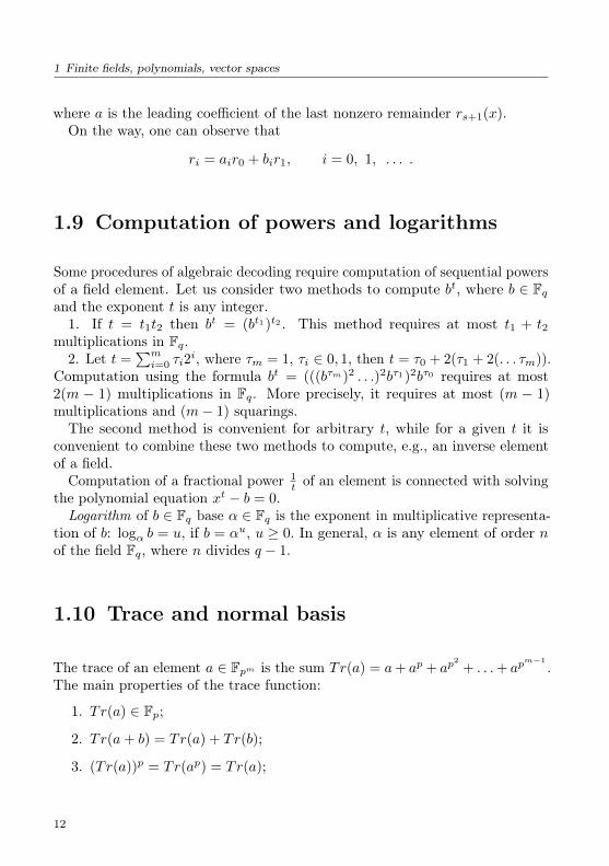
1.9 Computation of powers and logarithms
Some procedures of algebraic decoding require computation of sequential powersof a field element. Let us consider two methods to compute bt, where b ∈ Fqand the exponent t is any integer.1. If t = t1t2 then bt = (bt1)t2 . This method requires at most t1 + t2
multiplications in Fq.2. Let t =
∑mi=0 τi2
i, where τm = 1, τi ∈ 0, 1, then t = τ0 + 2(τ1 + 2(. . . τm)).Computation using the formula bt = (((bτm)2 . . .)2bτ1)2bτ0 requires at most2(m − 1) multiplications in Fq. More precisely, it requires at most (m − 1)multiplications and (m− 1) squarings.The second method is convenient for arbitrary t, while for a given t it is
convenient to combine these two methods to compute, e.g., an inverse elementof a field.
Computation of a fractional power 1t of an element is connected with solving
the polynomial equation xt − b = 0.Logarithm of b ∈ Fq base α ∈ Fq is the exponent in multiplicative representa-
tion of b: logα b = u, if b = αu, u ≥ 0. In general, α is any element of order nof the field Fq, where n divides q − 1.
1.10 Trace and normal basis
The trace of an element a ∈ Fpm is the sum Tr(a) = a+ ap + ap2
+ . . .+ apm−1
.The main properties of the trace function:
1. Tr(a) ∈ Fp;
2. Tr(a+ b) = Tr(a) + Tr(b);
3. (Tr(a))p = Tr(ap) = Tr(a);
12

1 Finite fields, polynomials, vector spaces
4. Tr(1) = m( mod p);
5. Tr(0) = 0;
6. Tr(β) = fi−1mt ( mod p),
where f(β) = 0, f(x) =∑ti=0 fix
i is the minimal polynomial of the element β;t divides m. The trace over any subfield Fq is defined similarly.
There are many applications of the trace function. The most important are:solving polynomial equations, building Galois fields, construction of sequencesover Fp with good correlation properties.A basis of a vector space is not unique. The most frequently used are
polynomial basis and normal basis. A normal basis is as follows: γ, γp, γp2
,. . . , γp
m−1
, γ ∈ Fpm . An important property of a normal basis is Tr(γ) 6= 0.For every field Fpm there exists a normal basis.
1.11 Ring of linearized polynomials
Denote [i] = qi mod m. Let q be a prime power. The polynomial
F (z) =
n∑i=0
Fiz[i],
where Fi ∈ Fqm , i = 0, 1, . . . , n is called linearized over the field Fqm . Denoteby Rm[z] the set of all such linearized polynomials. Let us define operations ofaddition and multiplication on this set.
1. Addition is defined in the same way as for ordinary polynomials: if
F (z) =
n∑i=0
Fiz[i], G(z) =
n∑i=0
Giz[i],
then
C(z) = F (z) +G(z) =
n∑i=0
(Fi +Gi)z[i]. (1.3)
The sum of linearized polynomials is a linearized polynomial.
13

1 Finite fields, polynomials, vector spaces
2. The operation of symbolic multiplication, denoted by ∗, differs from
multiplication of ordinary polynomials. If F (z) =n1∑i=0
Fiz[i] and G(z) =
n2∑k=0
Gkz[k], then
C(z) =n1+n2∑i=0
Ciz[i] = F (z) ∗G(z) = F (G(z))
=n1∑i=0
Fi(G(z))[i] =n1+n2∑j=0
( ∑i+k=j
FiG[i]k
)z[i+k].
(1.4)
Thus, the product C(z) of linearized polynomials is also a linearized polynomialwith coefficients Cj =
∑i+k=j
FiG[i+k]k . In contrast to ordinary multiplication,
the symbolic multiplication is a non-commutative operation: F (z) ∗ G(z) 6=G(z) ∗ F (z) in general. However the symbolic multiplication is associative:
F (z) ∗ (G(z) ∗H(z)) = (F (z) ∗G(z)) ∗H(z).
The defined operations are also distributive:
(F (z) +G(z)) ∗H(z) = F (z) ∗H(z) +G(z) ∗H(z),
H(z) ∗ (F (z) +G(z)) = H(z) ∗ F (z) +H(z) ∗G(z).
Hence, the set of linearized polynomials Rm[z] with the operations of additionand (symbolic) multiplication is a non-commutative ring. The unit of thering Rm[z] is the linearized polynomial e(z) = z. Indeed, for any polynomialF (z) ∈ Rm[z] it holds that z ∗ F (z) = F (z) ∗ z = F (z).
The q-degree of the polynomial F (z) =∑i Fiz
[i], denoted by qdeg(F ), is themaximum index i for which Fi 6= 0. This coefficient Fi is called the leadingcoefficient. If F (z) 6= 0 and G(z) 6= 0, then qdeg(F ∗G) ≥ qdeg(F ).
1.11.1 Left and right Euclidean algorithms
There are Euclidean algorithms for left and right divisions in the ring Rm[z]. Letus start with the left division. Let F1(z) =
∑ni=0 F1iz
[i] be any polynomial of
14

1 Finite fields, polynomials, vector spaces
q-degree qdeg(F1) = n and F0(z) =∑mk=0 F0kz
[k] be any polynomial of q-degreeqdeg(F0) = m > n. Subtract from F0(z) the polynomial F0mF
[n−m]1n zm−n ∗
F1(z). Then the q-degree of the difference D(z) will be less than m. If theqdeg(D) is at least n, then the leading coefficient of D(z) can be removedby subtracting correct left multiple of the polynomial F1(z). By continuingthis procedure, at the end we have F0(z) = G1(z) ∗ F1(z) + F2(z) where theremainder F2(z) is either the all zero polynomial or the polynomial of q-degreeless than n, i.e., qdeg(F2) < qdeg(F1).
The right division algorithm can be obtained by subtracting the right multiplesof the polynomial F1(z): F0(z) = F1(z) ∗Q(z) + f2(z), where either f2(z) = 0,or qdeg(f2) < qdeg(F1).Let us consider the left division in details. The right division is similar. Let
us write the sequence of equalities:
F0(z) = G1(z) ∗ F1(z) + F2(z), qdeg(F2) < qdeg(F1);F1(z) = G2(z) ∗ F2(z) + F3(z), qdeg(F3) < qdeg(F2);. . . . . . . . . . . . . . . . . . . . . . . . . . . . . . . . . . . . . .Fs−1(z) = Gs(z) ∗ Fs(z) + Fs+1(z), qdeg(Fs+1) < qdeg(Fs);Fs(z) = Gs+1(z) ∗ Fs+1(z).
(1.5)
Here, the last nonzero remainder Fs+1(z) is the right symbolic GCD of thepolynomials F0(z) and F1(z). If GCD is cz with c ∈ Fqm , then the polynomialsF0(z) and F1(z) are called coprime.Let us recurrently define polynomials Ui(z), Ai(z), Vi(z), Bi(z), for i ≥ 1:
Ui(z) = Ui−1(z) ∗Gi(z) + Ui−2(z), U0(z) = z, U−1(z) = 0,Ai(z) = Gi(z) ∗Ai−1(z) +Ai−2(z), A0(z) = z, A−1(z) = 0,Vi(z) = Vi−1(z) ∗Gi(z) + Vi−2(z), V0(z) = 0, V−1(z) = z,Bi(z) = Gi(z) ∗Bi−1(z) +Bi−2(z), B0(z) = 0, B−1(z) = z.
(1.6)
ThenF0(z) = Ui(z) ∗ Fi(z) + Ui−1(z) ∗ Fi+1(z),F1(z) = Vi(z) ∗ Fi(z) + Vi−1(z) ∗ Fi+1(z),
(1.7)
and
Fi(z) = (−1)i(Bi−1(z) ∗ F0(z)−Ai−1(z) ∗ F1(z)). (1.8)
15

1 Finite fields, polynomials, vector spaces
1.11.2 Factor ring of linearized polynomials
Together with the ring Rm[z] defined above let us consider its factor ring modulopolynomial z[m] − z consisting of the right residue classes. The elements of thefactor ring can be identified with linearized polynomials of q-degree at most[m− 1] = qm−1.
Let F (z) =∑m−1i=0 fiz
[i] ∈ Rm[z]. Then
F [1](z) = f[1]m−1z
[0] + f[1]0 z[1] + . . .+ f
[1]m−2z
[m−1].
Hence, q-powering of a polynomial in the ring Rm is equivalent to q-poweringof its coefficients followed by the right cyclic shift of the coefficients. We callthis operation a q-cyclic shift. Every ideal in the ring Rm[z] is the main idealgenerated by a polynomial G(z), which satisfies z[m] − z = H(z) ∗ G(z), i.e.,G(z) is the right divisor of the polynomial z[m] − z. Notice, if the leadingcoefficient of G(z) is 1, then polynomials G(z) and H(z) commute. The idealG is invariant with respect to q-cyclic shift, i.e., if g ∈ G, then g[i] ∈ Gas well.The two-sided ideal in the ring Rm[z], generated by z[m] − z, splits Rm[z]
into the set of residue classes modulo polynomial z[m] − z, isomorphic to thefacror ring Rm[z]/(z[m] − z). Denote this factor ring by Lm[z]. Elements ofLm[z] can be identified with all possible linearized polynomials over the fieldFqm with q-degree at most m− 1.
To do this, addition and multiplication of polynomials F (z) =m−1∑i=0
Fiz[i] and
G(z) =m−1∑i=0
Giz[i] from the ring Lm[z] should be defined as follows
F (z) +G(z) =
m−1∑i=0
(Fi +Gi)z[i] (1.9)
F (z)~G(z) = F (z) ∗G(z) mod z[m] − z. (1.10)
The ring Lm[z] is a finite non-commutative ring which consists of qm2
linearizedpolynomials. The Euclidean division algorithms in this ring are induced by thecorrespondent algorithms in Rm[z]. Hence all ideals in Lm[z] are main.
Consider the structure of a left ideal in details. Any such ideal is defined bya generator polynomial G(z), where G(z) is a divisor of z[m] − z. Elements of
16
1 Finite fields, polynomials, vector spaces
the ideal G are all possible polynomials of the form
g(z) = c(z)~G(z), (1.11)
where c(z) is any polynomial from Lm[z].If the generator polynomial has q-degree r, then the dimension of the ideal
equals k = m− r.Another way to define the ideal G uses the polynomial H(z) satisfying
z[m] − z = G(z) ∗H(z) as follows. A polynomial g(z) belongs to the ideal Gif and only if
g(z)~H(z) = 0. (1.12)
Indeed, if g(z) is the same as in (1.11), then
g(z)~H(z) = c(z)~G(z)~H(z) = c(z)~ (z[m] − z) = 0. (1.13)
Inversely, if (1.12) holds, then
g(z) ∗H(z) = c(z) ∗ (z[m] − z) = c(z) ∗G(z) ∗H(z). (1.14)
Hence, g(z) = c(z)~G(z).
Consider the polynomial
g(z) = g0z + g1z[1] + · · ·+ gm−2z
[m−2] + gm−1z[m−1]. (1.15)
Recall that q-cyclic shift of the polynomial is
g(z) = g[1]m−1z + g
[1]0 z[1] + g
[1]1 z[2] + · · ·+ gm−2z
[m−1]. (1.16)
If g(z) ∈ G(z) then z[1] ~ g(z) ∈ G(z). Hence, z[1] ~ g(z) = g(z)[1]
mod (z[m] − z) = g(z) ∈ G(z). Thus, if a polynomial belongs to the ideal,then all its q-cyclic shifts also belong to the same ideal.
17

2Rank metric codes
Introduction
Denote by Fq a finite field consisting of q elements, where q is a prime power.Later on, this field is called the base field. The extension of the field of degreem consists of qm elements and is denoted by Fqm .
There are two representations of codes in rank metric: matrix representationand vector representation.Matrix representation uses the space Fm×nq of rectangularm×nmatrices
over the base field Fq. Dimension of the space is mn.The norm N(M) of a matrix M ∈ Fm×nq is its algebraic rank over the field
Fq, N(M) = RkFq (M).The rank distance between two matrices M1,M2 ∈ Fm×nq is defined as the
norm of their difference: dr(M1, M2) = RkFq (M1 −M2).The matrix code M is a subset of the space Fm×nq of matrices.The rank code distance dr is the minimum rank distance between two different
code matrices:
dr = minRkFq (Mi −Mj) : Mi,Mj ∈M, i 6= j.
A matrix code M with code distance dr is Fq-linear if the code is a k-dimensional subspace of the space Fm×nq , where k ∈ 1, . . . ,mn. The code isnamed [m× n, k, dr]-code.
19

2 Rank metric codes
The cardinality of any matrix code M with m ≥ n and code distance drsatisfies the Singleton bound:
|M| ≤ qm(n−dr+1).
The dimension k of a Fq-linear [m× n, k, dr]-code satisfies: k ≤ m(n− dr + 1).If a matrix codeM reaches the Singleton bound, i.e.
|M| = qm(n−dr+1),
or for a linear codek = m(n− dr + 1),
then the code is called the maximum rank distance (MRD) code.
For the vector representation, the ambient space is the space Fnqm ofvectors of length n over the extension field Fqm .
Norm of a vector v ∈ Fnqm is the column rank of the vector
N(v) = RkFq (v),
which is defined as the maximum number of the vector components linearlyindependent over the base field Fq.
The rank distance between two vectors v1, v2 is defined as the norm of theirdifference: dr(v1, v2) = RkFq (v1 − v2).The vector code V is any subset of the vector space Fnqm.The rank code distance dr is the minimum rank distance between two different
code vectors:
dr = minRkFq (vi − vj) : vi,vj ∈M, i 6= j.
A vector code V with rank code distance dr is Fqm-linear if the code V isa k-dimensional subspace, k ∈ 1, 2, . . . , n, of the vector space Fnqm , wherescalars are elements of the extension field Fqm . The code is named [n, k, dr]-code.Fq-linear vector codes can also be defined, where codewords are elements ofFnqm and the scalars are elements of the base field Fq.
The cardinality |V| of any vector code with code distance dr and with m ≥ nsatisfies the Singleton bound:
|V| ≤ qm(n−dr+1).
For any Fqm -linear vector [n, k, dr]-code holds k ≤ n− dr + 1.
20

2 Rank metric codes
If a code reaches a Singleton bound then it is called an MRD code.
There exists close connection between vector and matrix codes. Let Ω =ω1, ω2, . . . , ωm be a basis of the extension field Fqm considered as a vectorspace over Fq. Take a vector v = (v1, v2, . . . , vj , . . . , vn), vj ∈ Fnqm . Every itscomponent can be uniquely written as
vj = a1,jω1 + a2,jω2 + · · ·+ ai,jωi + · · ·+ am,jωm,
where the coefficients ai,j are taken from the base field Fq. As a result, thevector v of length n over the extension field Fqm can be written as the m× nmatrix over the base field Fq by replacing every component vj by the columnvector (a1,j , a2,j , . . . , am,j)
T using a fixed basis Ω of the extension field. Inversemapping is also possible.
2.1 Delsarte matrix codes in rank metric
Delsate proposed codes in rank metric in the space of bi-linear forms. Let usdescribe these codes as matrix codes in the space of rectangular m× n matrices
Fm×nq , n ≤ m. The function Tr(x) =m−1∑l=0
xql
, x ∈ Fqm , is the trace function
from the extension field Fqm to the base field Fq.The Delsarte code is a Fq-linear [m×n, k, dr] MRD matrix code of dimension
k = m(n− dr + 1). The code is defined by the following parameters:
1. the rank code distance dr, 1 ≤ dr ≤ n,
2. the length k = n− dr + 1 of message vectors
u =[u0 u1 . . . un−dr
]∈ Fn−dr+1
qm ,
3. the subspace, spanned by elements N = ν1, ν2, . . . , νn from the exten-sion field Fqm linearly independent over Fq,
4. a basis Ω = ω1, ω2, . . . , ωm of the extension field Fqm .
The codeM is a set of m× n matrices. Every code matrix is defined by amessage vector u
M =M(u) : u ∈ Fn−dr+1
qm
,
21

2 Rank metric codes
where elements Mi,j(u), i = 1, 2, . . . ,m, j = 1, 2, . . . , n, of the matrix M(u)are given by
Mij(u) = Tr
(ωi
n−dr∑s=0
usνqs
j
).
The code distance dr of the codeM reaches the Singleton bound. Hence theDelsarte code is an MRD matrix code. General decoding methods for thesecodes are not described in existing publications in this field.
2.2 Dual bases
Recall, that for x ∈ Fqm the map σ(x) = xq is called the Frobenius automor-phism. This map preserves the base field: σ(Fq) = Fq. The map for vectors xand for matrices (Mij) is defined element-vise as follows:
σ(x) = xq = σ(x1, x2, . . . , xn) = (xq1, xq2, . . . , x
qn)
for x = (x1, x2, . . . , xn) ∈ Fnqm and
σ((Mij)) = (Mqij).
To construct MRD vector codes we need some of the properties of dual bases.Let components of the vector λ =
(λ1 λ2 . . . λm
)form a basis of the
extension field Fqm . The Moore matrix [Moo96] for this basis is
Λ =
λλq
λq2
. . .
λqm−2
λqm−1
=
λ1 λ2 . . . λmλq1 λq2 . . . λqmλq
2
1 λq2
2 . . . λq2
m
. . . . . . . . . . . .
λqm−2
1 λqm−2
2 . . . λqm−2
m
λqm−1
1 λqm−1
2 . . . λqm−1
m
.
This matrix is nonsingular [LN83].There is a unique dual basis µ =
(µ1 µ2 . . . µm
)such that the transpose
22

2 Rank metric codes
of its Moore matrix
M =
µµq
µq2
. . .
µqm−2
µqm−1
=
µ1 µ2 . . . µmµq1 µq2 . . . µqmµq
2
1 µq2
2 . . . µq2
m
. . . . . . . . . . . .
µqm−2
1 µqm−2
2 . . . µqm−2
m
µqm−1
1 µqm−1
2 . . . µqm−1
m
is inverse to the matrix Λ:
ΛM> =
λλq
λq2
. . .
λqm−2
λqm−1
(µ> (µq)
>. . .
(µq
m−2)> (
µqm−1
)>)=
=
λ1 λ2 . . . λmλq1 λq2 . . . λqmλq
2
1 λq2
2 . . . λq2
m
. . . . . . . . . . . .
λqm−2
1 λqm−2
2 . . . λqm−2
m
λqm−1
1 λqm−1
2 . . . λqm−1
m
µ1 µq1 . . . µq
m−2
1 µqm−1
1
µ2 µq2 . . . µqm−2
2 µqm−1
2
. . . . . . . . . . . . . . .
µm µqm . . . µqm−2
m µqm−1
m
= Im,
or equivalently for i = 1, 2, . . . ,m holds
λqi
·(µq
j)>
=
m∑s=1
λqi
s µqj
s =
1, if i = j;0, if i 6= j. (2.1)
2.3 MRD Gabidulin vector codes
Below we consider Fqm -linear maximum rank distance (MRD) vector codes overthe extension field Fqm of maximal possible length m. Shorter codes of lengthn < m can be obtained by deleting m− n columns from the generator or fromthe check matrix.
23

2 Rank metric codes
The rank metric [m, k, dr] vector code V can be defined by a full rank generatork ×m matrix Gk over the extension field Fqm . Code vectors are all possibleFqm -linear combinations of rows of the matrix.
Equivalently, this code can be defined by a full rank check (m−k)×m matrixHm−k over the extension field Fqm . The matrices should satisfy GkH
>m−k = 0,
where 0 is the all-zero k × (m− k) matrix. A vector code is an MRD code ifdr = m− k + 1. The following lemma allows us to verify this property.
Lemma 2.1 ([Gab85]). Let Hm−k ∈ F(m−k)×nqm be a check matrix of the code
V. The code V is an MRD code if and only if
RkFqm (YH>m−k) = m− k
for every matrix Y ∈ F(m−k)×mq over the base field with rank RFq (Y ) = m− k.
Another test is based on the known property [Gab85] that the dual code V⊥is also an MRD code with code distance d⊥r = k+ 1 and the generator matrix ofthe dual code V⊥ coincides with the check matrix Hm−k of the code V. Hencethe following lemma is true:
Lemma 2.2. Let Gk ∈ Fk×nqm be a generator matrix of the code V. The code Vis an MRD code if and only if
RkFqm (YG>k ) = k
for any matrix Y ∈ Fk×mq over the base field of rank RkFq (Y ) = k.
2.3.1 Vector codes based on dual bases
Theorem 2.3 ([Gab85]). Given dual bases λ and µ, the code V with generatorand check matrices
Gk =
λλq
λq2
...λq
k−2
λqk−1
, Hm−k =
µq
k
µqk+1
...µq
m−2
µqm−1
(2.2)
24

2 Rank metric codes
is an MRD code, i.e., it has cardinality qmk and code distance dr = m− k + 1.
Indeed, both matrices are of full rank. From bases duality and from (2.1) itfollows that Gk H>m−k = 0. Using Lemma 2.1 one can prove that the distanceof the code V is dr − 1 = m− k.
2.3.2 Generalized vector codes
The following theorem shows another class of vector codes.
Theorem 2.4 ([KG05]). Let s be a positive integer co-prime with the extensiondegree of the field, gcd(s,m) = 1. Then the code V with the following generatorand check matrices
Gk =
λλq
s
λq2s
...λq
(k−2)s
λq(k−1)s
, Hm−k =
µq
ks
µq(k+1)s
...µq
(m−2)s
µq(m−1)s
is an MRD code.
These codes are called generalized vector codes.The codes introduced in Theorems 2.3 and 2.4 are Fqm-linear vector codes
with the maximum rank distance, i.e., MRD-codes.
2.3.3 Vector codes based on linearized polynomials
Another way to construct rank metric vector codes is to use linearized polyno-mials. A linearized polynomial is a sum
u(x) = u0x+ u1xq + u2x
q2 + · · ·+ uk−1xqk−1
, (2.3)
where coefficients ui belong to the field Fqm .
25
2 Rank metric codes
Let us use the polynomial (2.3) to construct a vector code V. In order to dothis, select a basis λ =
(λ1 λ2 . . . λm
)and evaluate the polynomial (2.3)
“at the point” x = λ. In this way we obtain the following vector u(λ)
u(λ) =(u0 u1 . . . uk−1
)
λ
λq
...λq
k−1
,
which is a code vector of the code V. Here, one can see the message vectoru =
(u0 u1 . . . uk−1
)and the generator matrix Gk of the vector MRD
code.By evaluation all linearized polynomials of degree at most qk−1 at the point
x = λ we obtain all code vectors of the code V in Theorem 2.3.For many years, the only known MRD matrix codes were those of Delsarte
[Del78] and the vector MRD codes described in Theorems 2.3 and 2.4. Recently,new classes of vector MRD codes were suggested. In [She16], codes are definedusing another type of linearized polynomials:
u(x) = u0x+ u1xq + u2x
q2 + · · ·+ uk−1xqk−1
+ ηuqh
0 xqk
, (2.4)
where ui ∈ Fqm , i = 0, 1, . . . , k and the coefficients ui belong to the fieldFqm . The coefficient η also belong to Fqm , with the restriction that its normN(η) satisfies
N(η) = ηqm−1q−1 6= 1. (2.5)
For a basis λ =(λ1 λ2 . . . λm
)let us compute the vector
u(λ) = u0λ+ u1λq + u2λ
q2 + · · ·+ uk−1λqk−1
+ ηuqh
0 λqk .
This is one of the code vectors. By considering polynomials (2.4) with allpossible message coefficients u0, u1, . . . , uk−1 we obtain all the code vectorsu(λ) of the new code. The cardinality of the code is qmk and the rank codedistance is dr = m− k + 1, i.e., the new code is an MRD code.
The code construction based on the polynomial (2.4) gives Fqm -linear vectorcodes if the parameter h = 0. Otherwise, if h ≥ 1 it gives Fq-linear vector codes.
These codes are called twisted codes.
26

2 Rank metric codes
Remark 2.5. This construction can’t be used if q = 2, since any nonzeroelement η ∈ F2m has norm 1.
Another class of MDR codes obtained using the linearized polynomials
u(x) = u0x+u1xqs +u2x
q2s + · · ·+uk−1xq(k−1)s
+ ηuqh
0 xqks
, ui ∈ Fqm (2.6)
is described in the papers [She16, LTZ18]. Here s is a positive integer suchthat gcd(s,m) = 1 and the parameter η satisfies (2.5). These codes are calledgeneralized twisted codes.
The generator and check matrices of Fqm -linear twisted codes [She16] are asfollows
Gk =
λ+ ηλqk
λq
λq2
...λq
k−2
λqk−1
, Hm−k =
µq
k − ηµµq
k+1
...µq
m−2
µqm−1
. (2.7)
Similarly, the generator and check matrices of Fqm -linear generalized twistedcodes [LTZ18, She16] can be written as
Gk =
λ+ ηλqks
λqs
λq2s
...λq
(k−2)s
λq(k−1)s
, Hm−k =
µq
ks − ηµµq
(k+1)s
...µq
(m−2)s
µq(m−1)s
, gcd(s,m) = 1. (2.8)
New generalizations of Fqm -linear codes are proposed in the paper [PRS17]. Itis shown that such MRD codes exist for the code length n = 2−lm, where l isan integer and 2l|m. Explicit code construction uses the polynomials
u(x) = u0x+u1xq+· · ·+uk−1x
qk−1
+ηu0xqk−1+t
: ui ∈ Fqm , 1 < t < s−1. (2.9)
Among other recent constructions of MDR codes let us mention the codesdescribed in [OÖ16, OÖ17]. The paper [OÖ16] proposes (independently of
27

2 Rank metric codes
[She16]) Fq-linear MRD codes for the cases m = 3, dr = 2 and m = 4, dr = 3.The authors of [OÖ17] suggest a class of MRD codes under the name additivegeneralized twisted codes. If the base field is Fq = Fpu , where p is prime andu ≥ 2 is integer, then additive generalized twisted MRD codes are Fp-linear,but not necessarily Fq- or Fqm -linear.
The papers [She16, LTZ18, OÖ16, OÖ17, PRS17] do not consider any decod-ing methods to correct errors of restricted rank.
28

3q-cyclic rank metric codes
In this chapter, we introduce a code class that is similar to cyclic codes in theHamming metric.
Definition 1. A code M is called q-cyclic if together with any code vectorg =
(g0 g1 . . . gn−1
)it contains the vector g =
(g
[1]n−1 g
[1]0 . . . g
[1]n−2
),
obtained from g by the cyclic shift of its components by one position to the rightwith raising them to the q-th power.
Later on, we consider only linear q-cyclic rank metric codes. For simplicity,we will restrict ourselves to the case when n = m, i.e., when the code length ncoincides with the extension degree m of the field Fqm .
3.1 q-cyclic codes as ideals
Denote by Lm[z] the ring of linearized polynomials modulo z[m] − z.A linear (m, k)-codeM is q-cyclic if and only if it is a left ideal of the ring
Lm[z]. Since all ideals are principal in this ring, a q-cyclic (m, k)-code can bedefined by a generator polynomial G(z) of q-degree r = m− k. The polynomialG(z) divides z[m] − z:
H(z) ∗G(z) = z[m] − z. (3.1)
29

3 q-cyclic rank metric codes
Given the polynomial G(z), all code polynomials g(z) can be obtained usingthe rule
g(z) =
(k−1∑i=0
ciz[i]
)∗G(z) =
k−1∑i=0
ciG[i](z), (3.2)
where the coefficients ci, i = 0, 1, . . . , k − 1, independently take values from thefield Fqm .
3.2 Check polynomials
Another way to define a q-cyclic code is to use a check polynomial H(z) =H0z + · · ·+Hkz
[k], Hk = 1, obtained from (3.1). Code polynomials g(z) areall the solutions in the ring Lm[z] of the equation
g(z)~H(z) = 0. (3.3)
Encoding using the check polynomial is based on the relation (3.3), which canbe rewritten as(
m−k−1∑i=0
giz[i]
)~H(z) = −
(m−1∑i=m−k
giz[i]
)∗H(z). (3.4)
The q-degree of the polynomial in the left part of the equation is at mostm − 1. Hence, the operation of multiplication ~ in the ring Lm(z) can bereplaced by the operation of multiplication ∗ in the ring Rm(z).The encoding algorithm is as follows. We right multiply the “information
part” of a code polynomial
G0(z) = gm−kz[m−k] + · · ·+ gm−1z
[m−1]
by H(z) in the ring Lm(z), i.e., we reduce the product modulo z[m]− z. Havingobtained the polynomial we left divide byH(z) in the ringRm(z). The remaindergives “the check” part g0z+g1z
[1]+· · ·+g[m−k−1]z[m−k−1] of the code polynomial.
30

3 q-cyclic rank metric codes
3.3 Defining q-cyclic codes by roots
Let α1, α2, . . . , αr be a set of Fq-linear independent elements of the field Fqm .A q-cyclic code can be defined by these elements as follows.
The polynomial g(z) belongs to a q-cyclic (m, k)-code if and only if the rootsof the polynomial are all linear combinations u1α1 + u2α2 + · · · + urαr withcoefficients ui from Fq:
g(u1α1 + u2α2 + · · ·+ urαr) = 0. (3.5)
In fact, it is enough to require that
g(αs) = 0, s = 1, 2, . . . , r, (3.6)
since the polynomial g(z) is linearized and hence g(u1α1 +u2α2 + · · ·+urαr) =r∑s=1
usg(αs) for us ∈ Fq. So, if g(z) = g0z+· · ·+gm−1z[m−1] is a code polynomial,
thenm−1∑i=0
giα[i]s = 0, s = 1, 2, . . . , r. (3.7)
From here it follows that a check matrix of the q-cyclic code defined by theroots can be written as
H =
α
[0]1 α
[1]1 . . . α
[m−1]1
α[0]2 α
[1]2 . . . α
[m−1]2
...... . . .
...α
[0]r α
[1]r . . . α
[m−1]r
. (3.8)
In this case, the generator polynomial G(z) is the linearized polynomial ofminimal q-degree that has α1, α2, . . . , αr as the roots.
Example 4. Let r = 2. Let α1 = γ, α2 = γ[1], where γ is an element of anormal basis of the field Fqm . Then
H =
[γ γ[1] . . . γ[m−2] γ[m−1]
γ[1] γ[2] . . . γ[m−1] γ
].
The code defined by the check matrix H has distance 3 in rank metric.
31

3 q-cyclic rank metric codes
3.4 Generator matrices
In coordinate vector representation, a q-cyclic code can be defined by a generatormatrix G. Denote by c = (c0, c1, . . . , ck−1) a vector of information symbols.Then the correspondent code vector g is
g = cG. (3.9)
Sometimes it is convenient to have a systematic encoding, where componentsof the information vector c can be found at fixed positions of the code vector.In a q-cyclic code, the information symbols can be placed at any k sequentialposition. It is convenient to place the information symbols to k leading positionsm− 1, m− 2, . . . , m− k. In this case, the generator matrix can be obtained asfollows. Divide in the ring Rm[z] the monomial z[i] by the generator polynomialG(z) :
z[i] = Qi(z) ∗G(z) +Ri(z). (3.10)
Thenz[i] −Ri(z) = Qi(z) ∗G(z) (3.11)
are code polynomials. For i = m− 1, m− 2, . . . , m− k, these polynomialsand correspondent vectors are linearly independent. These vectors form therows of the generator matrix:
G = (−R Ik). (3.12)
Here Ik is the identity matrix of order k, and R is the k × (m− k) matrix inwhich i-th row is the remainder Rm−i(z) in the vector representation.
This encoding of a q-cyclic code can be implemented using the Euclideanalgorithm as follows. Denote the information symbols
cr−1 = gm−1, ck−2 = gm−2, . . . , c0 = gm−k
and the polynomial
G0(z) = gm−1z[m−1] + gm−2z
[m−2] + · · ·+ gm−kz[m−k].
Using right division of this polynomial by the generator polynomial G(z) obtain
G0(z) = Q(z) ∗G(z) + F (z), qdeg(F ) < qdeg(G) = m− k. (3.13)
32

3 q-cyclic rank metric codes
Then the coefficients gm−i, i = k + 1, . . . , m of the remainder F (z) give theremaining (check) symbols of the code vector:
g =
(g0, g1, . . . , gm−k−1︸ ︷︷ ︸, ︷ ︸︸ ︷
gm−k, . . . , gm−1
).
3.5 Check matrices
The check matrix H is defined by the check polynomial H(z) =k∑i=0
Hiz[i] and
has the form
H =
Hk H
[1]k−1 . . . H
[k]0 0
. . . 0
0 H[1]k . . . H
[k]1 H
[k+1]0 0 0
. . . . . . . . . . . . . . . . . . 0
0 0 . . . 0 H[r−1]k . . . H
[m−1]0
=
hk hk−1 . . . h0 0
. . . 0
0 h[1]k . . . h
[1]1 h
[1]0 0 0
. . . . . . . . . . . . . . . . . . 0
0 0 . . . 0 h[r−1]k . . . h
[r−1]0
,(3.14)
where we denote hi = H[k−i]i , i = 0, 1, . . . , k.
33


4Fast algorithms for decoding rankcodes
4.1 Error correction in rank metric
Codes with check matrix (2.2) allows error correction using the algorithmssimilar to decoding algorithms for generalized Reed–Solomon codes.Let g = (g1, . . . , gn) be a code vector, e = (e1, . . . , en) an error vector, and
y = g + e the received vector. Compute the syndrome
s = (s0, s1, . . . , sd−2) = yHT = eHT . (4.1)
The task of the decoder: given the syndrome s find an error vector. Let therank norm of the error vector be t. Then it can be written as
e = EY = (E1, . . . , Et)Y, (4.2)
where E1, . . . , Et are linearly independent over Fq, and Y = (Yij) is an (t× n)-matrix of rank t with elements from Fq. Then (4.1) can be rewritten as
s = EYHT = EX, (4.3)
35

4 Fast algorithms for decoding rank codes
where the matrix X = YHT has the form
X =
x1 x
[1]1 . . . x
[d−2]1
x2 x[1]2 . . . x
[d−2]2
. . . . . . . . . . . . .
xt x[1]t . . . x
[d−2]t
,where
xp =
n∑j=1
Ypjhj , p = 1, . . . , t, (4.4)
are linearly independent over Fq. Equation (4.1) is equivalent to the followingsystem of equations with unknowns E1, . . . , Et, x1, x2, . . . , xt:
t∑i=1
Eix[p]i = sp, p = 0, 1, . . . , d− 2. (4.5)
Let a solution of the system be found. Then from (4.4) a matrix Y can becalculated, and from (4.2) an error vector e can be obtained. Note that thesystem (4.5) for a given t has many solutions, however for t ≤ (d−1)
2 all solutionslead to the same vector e.
So, the decoding problem is reduced to solving system (4.5) for the minimalt.
Define the polynomial S(z) =∑d−2j=0 sjz
[j]. Let ∆(z) =∑tp=0 ∆pz
[p], ∆t = 1,denote a polynomial that has all possible Fq-linear combinations of E1, E2, . . . , Et
as roots. Let F (z) =∑t−1i=0 Fiz
[i], where Fi =∑ip=0 ∆ps
[p]i−p, i = 0, 1, . . . , t− 1.
Lemma 4.1. The following equality holds
F (z) = ∆(z) ∗ S(z) mod z[d−1]. (4.6)
Indeed,
∆(z) ∗ S(z) =
t∑p=0
∆p(S(z))[p] =
t+d−2∑i=0
z[i]
∑p+j=i
∆ps[p]j
.
For t ≤ i ≤ d− 2 we have∑p+j=i ∆ps
[p]j =
∑tp=0 ∆ps
[p]i−p =
∑tp=0 ∆p
(∑tj=1Ejx
[j−p]j
)[p]
=
=∑tj=1 x
[i]j ∆(Ej) = 0
36

4 Fast algorithms for decoding rank codes
since ∆(Ej) = 0, j = 1, 1, . . . , t.
If the coefficients of F (z) are known, then the coefficients of the polynomial∆(z) can be found recurrently as follows. Let s0 = . . . = sj−1 = 0, sj 6= 0. Then
∆0 =Fjsj,
∆p =
(Fj+p−
∑p−1i=0 ∆is
[i]p+j−i
)s[p]j
, p = 1, 2, . . . , t,
(4.7)
where for j + p ≥ t we set Fj+p = 0.Now assume that E1, . . . , Et and the polynomial ∆z are known. Consider
the “shortened” system of equations
t∑j=1
Ejx[p]j = sp, p = 0, 1, . . . , t− 1 (4.8)
with unknowns x1, x2, . . . , xt.Let us solve (4.8) by sequential exclusion of variables. Denote A1j =
Ej , Q1p = sp. Multiply the (p+ 1)-th equation of the system by Aq−111 , take the
root of order q and subtract it from p-th equation. As a result, obtain a systemwithout x1:
p∑j=2
A2jx[p]j = Q2p, p = 0, 1, . . . ,m− 2, (4.9)
where
A2j = A1j −(A1j
A11
)[−1]
A11, j = 2, . . . , t,
Q2p = Q1p −(Q1p+1
A11
)[−1]
A11, p = 0, 1, . . . , t− 2.
(4.10)
By repeating this procedure t − 1 times and leaving the first equations inthe system at every step we get a system of linear equations with a triangularmatrix of coefficients:
t∑j=1
Aijxj = Qi0, i = 1, 2, . . . , t, (4.11)
37

4 Fast algorithms for decoding rank codes
where
A1j = Ej , j = 1, . . . , ;
Aij =
0, j < i,
Ai−1,j −(
Ai−1,j
Ai−1,i−1
)[−1]
Ai−1,i−1, p = 0, . . . , t− i, i = 2, . . . , t.
(4.12)Q1p = sp, p = 0, . . . , t− 1,
Qip = Qi−1,p −(Qi−1,p+1
Ai−1,i−1
)[−1]
Ai−1,i−1, p = 0, 1, . . . , t− i, i = 2, . . . , t.
(4.13)System (4.11) can be solved using the following recurrent formulas
xt = Qt0Amm
,
xt−i =(Qt−i,0−
∑tj=t−i+1 A−i,j)
At−i,t−i, i = 1, . . . , t− 1.
(4.14)
The decoding algorithm is as follows.I. Compute the syndrome vector s = (s0, . . . , sd−2) and obtain correspondent
polynomial S(z) =∑d−2i=0 siz
[i].II. Set F0(z) = z[i−1], F1(z) = S(z), and apply the Euclidean algorithm until
Ft+1(z) is such thatqdeg(Ft(z)) ≥ q
d−12 . (4.15)
Then∆(z) = γA(z),
F (z) = γ(−1)tFt+1(z),
(4.16)
where γ is selected such that the coefficient ∆t is equal to 1.Indeed, if the number of rank errors is at most (d−1)
2 , then equalities (4.16)follow from (1.8) and from Lemma 4.1. The uniqueness of polynomials F (z)and ∆(z) can be proved in the same way as in the case of standard generalizedReed–Solomon codes.The polynomial ∆(z) can be found either by the first formula in (4.16), if
the polynomials Ai(z), i = 1, 2, . . . , have been computed using the Euclideanalgorithm, or using (4.7), where the coefficients of remainders Fm+1(z), com-puted with the algorithm, are required. Then any Fq-linearly independent rootsE1, . . . , Em of the polynomial ∆(z) can be found.
38
4 Fast algorithms for decoding rank codes
III. Using (4.11)-(4.14) and known E1, . . . , Et compute x1, . . . , xt. Find thematrix Y from decomposition (4.4). Finally, compute the error vector e from(4.2).
As an example, consider the case d = 3, q = 2. Here we can correct singlerank errors in a field of characteristic 2.
1. Compute the syndrome s = (s0, s1). If s0 = 0 and s1 = 0 then concludethat there were no errors.
2. If s0 6= 0 and s1 6= 0 then the Euclidean algorithm gives the polynomial∆(z) = −(
s10s[1]
)z + z[1]. Conclude that it was a single error and find E as
a nonzero root of the equation ∆(z) = 0, i.e., E = (s[1]0
s1). In this case, the
system (4.10) has a single equation and gives x = s1s0
= y1h1 + y2h2 + . . .+ynhn, where yi = 0 or 1. The error vector is e = (y1E, y2E, . . . , ynE).
3. If s0 = 0, s1 6= 0 or s0 6= 0, s1 = 0, then conclude that the error has arank at least 2 since the Euclidean algorithm would give the polynomials∆(z) = z[1] and ∆(z) = z[2], which have no roots.
4.2 Error and erasure correction by MRD codes
Assume we need to correct errors and also erasures of columns and rows upto the theoretical bound. If there have been no erasures then the decodingalgorithm from Section 4.1 will correct rank errors.
Later we will show that in general the variables corresponding to row erasurescan be excluded from the (first) system of syndrome equations, giving the secondsystem, and the decoding problem will be reduced to error and column erasurecorrection. In turn, the column erasures can be excluded from the secondsystem of syndrome equations in a similar way, and the decoding problem willbe reduced to error correction only. After error correction we will return tocolumn erasure correction and then to row erasures. As a result, we will correctall three types of distortions: errors and erasures of both columns and rows.
Before we describe the general decoding algorithm let us recall the constructionof the rank distance (n, k, d)-code, where n is the code length, k is the numberof information symbols, and d is the code distance.
39

4 Fast algorithms for decoding rank codes
The rank of a vector x = (x0, x1, . . . , xn−1), xj ∈ Fqn , denoted by RkFq(x),is the maximum number of components that are linearly independent over Fq.
Let the vectorg = (g0, g1, ..., gn−1) (4.17)
give a basis of the extension Fqn of the base field Fq, i.e., components gj ∈Fqn , j = 0, . . . , n− 1, are linearly independent over the base field Fq. Then anyn-vector x ∈ Fnqn can be uniquely represented as
x = (x0, x1, . . . , xn−1) = (g0, g1, ..., gn−1)A(x) = gA(x), (4.18)
where A(x) is a n× n matrix over the base field Fq.Equivalently, the rank of a vector x can be defined as the standard algebraic
rank of the matrix A(x), i.e., RkFq (x) = Rk(A(x)).
A code in vector representation (vector code) with rank distance d is definedas a set V ⊆ Fnqn of vectors xj ∈ Fnqn such that min
i 6=jRkFq (xi − xj) = d.
The same code in matrix form (matrix code) is the set of correspondingmatrices A(xj), j = 1, . . . , V .An Fqn-linear code with rank distance d having V = (qn)k code vectors we
denote by (n, k, d)-code. An (n, k, d)-code is called the maximum rank distance(MRD) code if d = n− k + 1.
An MRD (n, k, d = n − k + 1) code in vector form can be defined by agenerator matrix. The standard form of a generator matrix is:
Gk =
g0 g1 . . . gn−1
g[1]0 g
[1]1 . . . g
[1]n−1
. . . . . . . . . . . .
g[k−1]0 g
[k−1]1 . . . g
[k−1]n−1
, (4.19)
where g[i]j = gq
i mod n
j .The first row of the generator matrix is the vector
g = (g0, g1, ..., gn−1),
over the extension field Fqn , where the components gj ∈ Fqn , j = 0, . . . , n− 1,are linearly independent over the base field Fq. Hence, the vector g is a basis ofthe extension field Fqn over the base field Fq. Every next row of the generatormatrix is the Frobenius power of the previous row.
40

4 Fast algorithms for decoding rank codes
Denote by u = (u0, u1, . . . , uk−1) the information vector, which has informa-tion symbols, uj ∈ Fqn , j = 0, 1, . . . , k− 1 as components. Then the code vectorg(u) corresponding to the information vector u can be obtained as
g(u) = uGk. (4.20)
The rank norm of any nonzero code vector is at least n− k + 1, hence the codedistance is d = n− k + 1.Known fast decoding algorithms use the following check matrix
Hn−k = Hd−1 =
h0 h1 . . . hn−1
h[1]0 h
[1]1 . . . h
[1]n−1
. . . . . . . . . . . .
h[n−k+1]0 h
[n−k+1]1 . . . h
[n−k+1]n−1
, (4.21)
where elements h0, h1, . . . , hn−1 are linearly independent over the base field Fq.The generator and the check matrices satisfy
GkH>n−k = 0. (4.22)
4.3 Rank errors and rank erasures
Rank metric codes can be used for telecommunication as follows.Select an MRD (n, k, d)-code in vector form. The vector form is convenient
for coding and decoding. A code word g(u) to be transmitted is convertedusing (4.18) to a square q-ary matrix of order n. For definiteness assume thatthe first row of the generator matrix Gk is the basis of the extension field.The code matrix is transmitted over a system of n parallel channels. Ele-
ments of the i-th row enter the i-th channel. Elements of the j-th column aretransmitted during the j-th time interval.
The code matrix can be distorted during the transmission by adding a noisematrix of order n. Consider three types of distortions.
1. The noise matrix E is added to the code matrix and the receiver doesnot know which columns or rows are distorted. The received matrix istransformed to a vector using (4.18). Hence, the decoder should processthe received vector
y = g(u) + e.
41

4 Fast algorithms for decoding rank codes
We say that there is an error of rank m, or m rank errors, if RkFq (e) = m.To be corrected, the error of rank m is written as
e = (e1, e2, . . . , em)U, (4.23)
where the unknown elements ej ∈ Fqn , are Fq-linearly independent and Uis a q-ary m× n matrix
U =
u1,1 u1,2 . . . u1,n
u2,1 u2,2 . . . u2,n
...... . . .
...um,1 um,2 . . . um,n
(4.24)
with unknown elements.
2. The noise matrix Erow is added to the code matrix and the receiver knowsthe side information that the rows i1, i2, . . . , iv can be distorted. Thereceived matrix is transformed to a vector using (4.18). If only the i-throw R of Erow is nonzero then the code vector is distorted by giR, wheregi is a known basis element. Hence, the decoder should work with thevector
y = g(u) + erow,
whereerow = (gi1 , gi2 , . . . , giv )Rrow. (4.25)
Here the elements gij are known, while the q-ary v × n matrix
Rrow =
r1,1 r1,2 . . . r1,n
r2,1 r2,2 . . . r2,n
...... . . .
...rv,1 rv,2 . . . rv,n
(4.26)
is unknown. We say that the vector erow defines an erasure of v rows.
3. The noise matrix Ecol is added to the code matrix and the receiver knowsthe side information that the columns j1, j2, . . . , jr can be distorted. Thereceived matrix is transformed to a vector using (4.18). If only the j-thcolumn of Ecol is nonzero then Ecol will be transformed to the vector wjc,where wj ∈ Fqn is an unknown while c is a known q-ary n-vector that
42

4 Fast algorithms for decoding rank codes
has the j-th component 1 and all the rest are zeros. Hence, the decodershould work with the vector
y = g(u) + ecol,
whereecol = (wj1 , wj2 , . . . , wjr )Ccol. (4.27)
Here wjk are unknown while the q-ary r × n matrix
Ccol =
0 . . . 0 c1,j1 = 1 0 . . . 00 . . . . . . 0 c2,j2 = 1 . . . 00 . . . . . . . . . . . . . . . 00 . . . . . . . . . 0 cr,jr = 1 . . .
(4.28)
is known. We say that the vector ecol defines erasure of r columns.
In the general case, rank errors and erasures can occur simultaneously and adecoder should process the received vector
y = g(u) + e + erow + ecol (4.29)
where the error vectors are given in (4.23), (4.25) and (4.27).
Lemma 4.2. An MRD (n, k, d = n−k+1) code corrects simultaneously erasuresof v rows, r columns and errors of rank m if
2m+ v + r ≤ d− 1. (4.30)
Proof. Consider all the code matrices of order n. Delete v rows and r columnsin all these matrices. We obtain a new code of (n− v)× (n− r) matrices withrank distance at least d = d− v − r. Hence, this code corrects errors of rank mif m ≤ (d− v − r − 1)/2, or
2m+ v + r ≤ d− 1.
Simultaneous error and erasure correction is considered in the next section
43

4 Fast algorithms for decoding rank codes
4.4 Simultaneous error and erasure correction
Consider an algorithm for error and erasure correction. The algebraic decodingstarts with computation of the syndrome vector s = (s0, s1, . . . , sd−2). For areceived vector y, given by (4.29), we have
s> =
s0
s1
...sd−2
= Hd−1y>
= Hd−1U>
e1
e2
...em
+ Hd−1R>row
gi1gi2...giv
+ Hd−1C>col
wj1wj2...wjr
.
(4.31)
Using (4.24), (4.26) and (4.28) we can rewrite the syndrome as follows
s>=
s0
s1
...sd−2
=
m∑k=1
ek
xk
x[1]k
...x
[d−2]k
+
v∑k=1
gik
fk
f[1]k...f
[d−2]k
+
r∑k=1
wjk
hjkh
[1]jk
...h
[d−2]jk
.
(4.32)Here xk =
∑np=1 hp−1uk,p, k = 1, . . . ,m, fk =
∑np=1 hp−1rk,p, k = 1, . . . , v.
Without loss of generality we can assume that the elements of each of thefollowing sets
x1, . . . , xm, f1, . . . , fv, hj1 , . . . , hjrand
e1, . . . , em, gi1 , . . . , giv , wj1 , . . . , wjr(4.33)
are linearly independent over Fq. Otherwise the number of unknowns canbe decreased. The decoding can be done using the syndrome (4.32) and itsmodifications.
44

4 Fast algorithms for decoding rank codes
Together with the syndrome s let us use the modified syndrome smod:
s>mod =
s
[n]0
s[n−1]1...s
[n−d+2]d−2
=
m∑k=1
xk
e
[n]k
e[n−1]k...e
[n−d+2]k
+
v∑k=1
fk
g
[n]ik
g[n−1]ik...g
[n−d+2]ik
+
r∑k=1
hjk
w
[n]jk
w[n−1]jk
...w
[n−d+2]jk
.
(4.34)
The decoder should solve system of equations (4.32) or (4.34) and findunknowns xk, fk, ek, wjk. After this, rank errors e and rank erasures erow, ecol
should be corrected.Let us show that it is possible if conditions of Lemma 4.2 are satisfied. The
idea is as follows.First assume that there were no erasures, i.e., erow = ecol = 0 and only rank
errors should be corrected. In this case, the syndrome (4.32) contains unknownsxk, ek only. Existing standard algorithms allow rank error correction if therank m satisfies 2m ≤ d− 1.Let us show that in the general case, the unknowns fk, that define row
erasures, can be excluded from the system of equations (4.32). The problemwill be reduced to correction of rank errors and column erasures. In turn, thecolumn erasures also can be excluded and we only need to correct errors.
4.4.1 Exclusion of row erasures
Row erasures are included in in the syndrome as:
v∑k=1
gik
fk
f[1]k...f
[d−2]k
,
45

4 Fast algorithms for decoding rank codes
where the elements gik , k = 1, . . . , v, are known while fk, k = 1, . . . , v, areunknown.Define the linearized polynomial
T (z) =
v∑i=0
Tiz[i], (4.35)
that has all Fq-linear combinations of gik , k = 1, . . . , v, as roots. In particular,
T (gik) = 0, k = 1, 2, . . . , v. (4.36)
The coefficients Ti are used to exclude unknowns fk, k = 1, . . . , v, and tomodify the syndrome. Denote the modified syndrome by s = (s0 s1 . . . sd−2−v).It has dimension d− 1− v and can be computed as follows:
s> =
s0
s1
...sd−3−vsd−2−v
=
sv s[1]v−1 . . . s
[v−1]1 s
[v]0
sv+1 s[1]v . . . s
[v−1]2 s
[v]1
...... · · ·
......
sd−3 s[1]d−4 . . . s
[v−1]d−4−v s
[v]d−3−v
sd−2 s[1]d−3 . . . s
[v−1]d−3−v s
[v]d−2−v
T0
T1
...Tv−1
Tv
.
(4.37)Denote:
ek = T (ek); xk = x[v]k ; k = 1, 2, . . . ,m;
wjk = T (wjk); hjk = h[v]jk
; k = 1, 2, . . . , r.(4.38)
Lemma 4.3. The modified syndrome s can be written as:
s> =
s0
s1
...sd−2−v
=
m∑k=1
ek
xk
x[1]k
...x
[d−2−v]k
+
r∑k=1
wjk
hjkh
[1]jk
...h
[d−2−v]jk
. (4.39)
46

4 Fast algorithms for decoding rank codes
Proof. From (4.32) and (4.37) we get
sj = sv+jT0 + s[1]v+j−1T1 + · · ·+ s
[v−1]j+1 Tv−1 + s
[v]j Tv =(
m∑k=1
ekx[v+j]k +
v∑k=1
gikf[v+j]k +
r∑k=1
wjkh[v+j]jk
)T0 +(
m∑k=1
e[1]k x
[v+j]k +
v∑k=1
g[1]ikf
[v+j]k +
r∑k=1
w[1]jkh
[v+j]jk
)T1 +
... +(m∑k=1
e[v]k x
[v+j]k +
v∑k=1
g[v]ikf
[v+j]k +
r∑k=1
w[v]jkh
[v+j]jk
)Tv =(
m∑k=1
T (ek)x[v+j]k +
v∑k=1
T (gik)f[v+j]k +
r∑k=1
T (wjk)h[v+j]jk
)=(
m∑k=1
T (ek)x[v+j]k +
r∑k=1
T (wjk)h[v+j]jk
)=(
m∑k=1
ekx[j]k +
r∑k=1
wjk h[j]jk
).
Here conditions (4.36) and notations (4.38) were used.
From (4.39) it follows that row erasures are temporary excluded. The decodershould correct errors of rank m and column erasures of rank r. The next stepis to exclude column erasures.
47
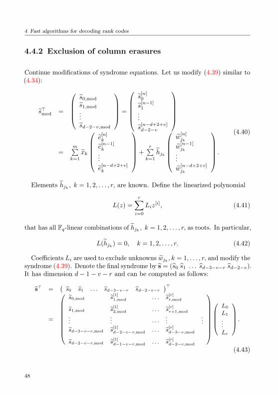
4 Fast algorithms for decoding rank codes
4.4.2 Exclusion of column erasures
Continue modifications of syndrome equations. Let us modify (4.39) similar to(4.34):
s>mod =
s0,mod
s1,mod
...sd−2−v,mod
=
s
[n]0
s[n−1]1...s
[n−d+2+v]d−2−v
=m∑k=1
xk
e
[n]k
e[n−1]k...e
[n−d+2+v]k
+r∑
k=1
hjk
w
[n]jk
w[n−1]jk
...w
[n−d+2+v]jk
.
(4.40)
Elements hjk , k = 1, 2, . . . , r, are known. Define the linearized polynomial
L(z) =
r∑i=0
Liz[i], (4.41)
that has all Fq-linear combinations of hjk , k = 1, 2, . . . , r, as roots. In particular,
L(hjk) = 0, k = 1, 2, . . . , r. (4.42)
Coefficients Li are used to exclude unknowns wjk , k = 1, . . . , r, and modify thesyndrome (4.39). Denote the final syndrome by s = (s0 s1 . . . sd−3−v−r sd−2−v).It has dimension d− 1− v − r and can be computed as follows:
s> =(
s0 s1 . . . sd−3−v−r sd−2−v−r
)>
=
s0,mod s[1]1,mod . . . s
[r]r,mod
s1,mod s[1]2,mod . . . s
[r]r+1,mod
...... · · ·
......
sd−3−v−r,mod s[1]d−2−v−r,mod . . . s
[r]d−3−v,mod
sd−2−v−r,mod s[1]d−1−v−r,mod . . . s
[r]d−2−v,mod
L0
L1
...Lr
.
(4.43)
48

4 Fast algorithms for decoding rank codes
Lemma 4.4. The final syndrome s can be written as:
s> =
s0
s1
...sd−3−v−rsd−2−v−r
=
m∑k=1
ek
x
[n]k
x[n−1]k
...x
[n−d+2+v+r]k
, (4.44)
whereek = L(xk); k = 1, 2, . . . ,m;xk = ek; k = 1, 2, . . . ,m.
(4.45)
Proof. From (4.40) (4.43) we get
sj = sj,modL0 + s[1]j+1,modL1 + · · ·+ s
[r−1]j+r−1,modLr−1 + s
[r]j+r,modLr =(
m∑k=1
xke[n−j]k +
r∑k=1
hjk w[n−j]jk
)L0 +(
m∑k=1
x[1]k e
[n−j]k +
r∑k=1
h[1]jkw
[n−j]jk
)L1 +
. . . +(m∑k=1
x[r]k e
[n−j]k +
r∑k=1
h[r]jkw
[n−j]jk
)Lr =(
m∑k=1
L(xk)e[n−j]k +
r∑k=1
L(hjk)w[n−j]jk
)=
m∑k=1
L(xk)e[n−j]k =
m∑k=1
ekx[n−j]k .
Here we use conditions (4.42) and notations (4.45).
Equations (4.44) allow us to compute errors of rank m if 2m ≤ d− 1− v − r.
4.4.3 Short description of the algorithm correcting errorsand erasures simultaneously
The basic steps of the algorithm are as follows.
49
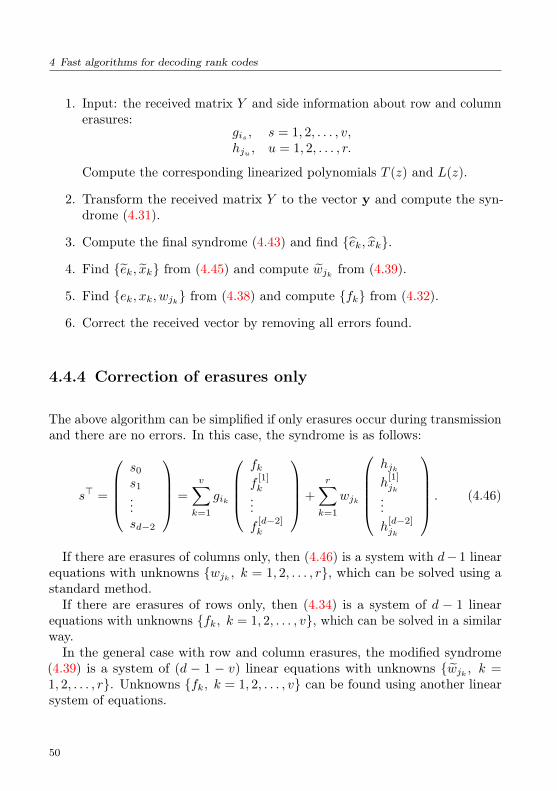
4 Fast algorithms for decoding rank codes
1. Input: the received matrix Y and side information about row and columnerasures:
gis , s = 1, 2, . . . , v,hju , u = 1, 2, . . . , r.
Compute the corresponding linearized polynomials T (z) and L(z).
2. Transform the received matrix Y to the vector y and compute the syn-drome (4.31).
3. Compute the final syndrome (4.43) and find ek, xk.
4. Find ek, xk from (4.45) and compute wjk from (4.39).
5. Find ek, xk, wjk from (4.38) and compute fk from (4.32).
6. Correct the received vector by removing all errors found.
4.4.4 Correction of erasures only
The above algorithm can be simplified if only erasures occur during transmissionand there are no errors. In this case, the syndrome is as follows:
s> =
s0
s1
...sd−2
=
v∑k=1
gik
fk
f[1]k...f
[d−2]k
+
r∑k=1
wjk
hjkh
[1]jk
...h
[d−2]jk
. (4.46)
If there are erasures of columns only, then (4.46) is a system with d− 1 linearequations with unknowns wjk , k = 1, 2, . . . , r, which can be solved using astandard method.If there are erasures of rows only, then (4.34) is a system of d − 1 linear
equations with unknowns fk, k = 1, 2, . . . , v, which can be solved in a similarway.
In the general case with row and column erasures, the modified syndrome(4.39) is a system of (d − 1 − v) linear equations with unknowns wjk , k =1, 2, . . . , r. Unknowns fk, k = 1, 2, . . . , v can be found using another linearsystem of equations.
50

4 Fast algorithms for decoding rank codes
4.5 Examples
As an example let us consider a MRD (5, 1, 5)-code over F25 . with the generatormatrix
G = (αα30 α18 α7 α20).
A check matrix is :
H4 = Hd−1 =
α2 α29 α5 α14 α9
α4 α27 α10 α28 α18
α8 α23 α20 α25 α5
α16 α15 α9 α19 α10
. (4.47)
These matrices are connected by the equation: GH>4 = 0.
If the information symbol u = 1 then the code vector is
g(u) = (αα30 α18 α7 α20).
The corresponding code matrix M(u) is
M(u) =
0 0 1 0 01 1 1 0 00 0 0 1 10 0 0 0 10 1 0 1 0
.
Let us consider some variants of errors and erasures.
Variant 1: 1 error and 2 erasuresLet the noise matrix be
E =
0 0 1 1 11 1 0 0 00 1 0 0 01 1 0 0 01 0 0 0 0
.
51
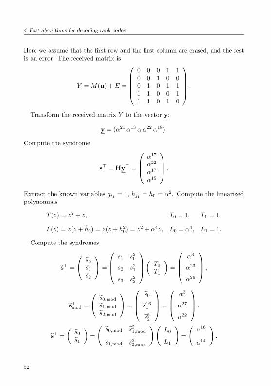
4 Fast algorithms for decoding rank codes
Here we assume that the first row and the first column are erased, and the restis an error. The received matrix is
Y = M(u) + E =
0 0 0 1 10 0 1 0 00 1 0 1 11 1 0 0 11 1 0 1 0
.
Transform the received matrix Y to the vector y:
y = (α21 α13 αα22 α18).
Compute the syndrome
s> = Hy> =
α17
α22
α17
α15
.
Extract the known variables gi1 = 1, hj1 = h0 = α2. Compute the linearizedpolynomials
T (z) = z2 + z, T0 = 1, T1 = 1.
L(z) = z(z + h0) = z(z + h20) = z2 + α4z, L0 = α4, L1 = 1.
Compute the syndromes
s> =
s0
s1
s2
=
s1 s2
0
s2 s21
s3 s22
( T0
T1
)=
α3
α23
α26
,
s>mod =
s0,mod
s1,mod
s2,mod
=
s0
s161
s82
=
α3
α27
α22
.
s> =
(s0
s1
)=
(s0,mod s2
1,mod
s1,mod s22,mod
)(L0
L1
)=
(α16
α14
).
52

4 Fast algorithms for decoding rank codes
Find e1,x1:
s> =
(α16
α14
)= e1
(x1
x161
),
e1x1 = α16,
e1x161 = α14.
e1 = α12,
x1 = α4.
To find errors we solve the following equations:
x21 + α4x1 = e1 = α12 −→ x1 = α16.
e1 = x1 = α4, x1 = x21 = α16 −→ x1 = α8.
e1 = e21 + e1 = α4 −→ e1 = α12.
(u1 u2 u3 u4 u5)(α2 α29 α5 α14α9)> = x1 −→(u1 u2 u3 u4 u5) = (1 1 0 0 0) −→
e = (α12 α12 0 0 0)
To find column erasures we solve the following equations:
s0 = α3 = e1x1 + w1h0 = α4α16 + α4w1 −→ w1 = α29.
w21 + w1 = w1 = α29 −→ w1 = α22.
ecol = (α22 0 0 0 0)
To find row erasures we solve the following equations:
s0 = α7 = e1x1 + g1f1 + w1h0 = α12α8 + 1 · f1 + α22α2 −→ f1 = α19.
(α2 α29 α5 α14α9)(r1 r2 r3 r4 r5)> = f1 −→(r1 r2 r3 r4 r5) = (1 0 1 1 1) −→
erow = (1 0 1 1 1)
The total error vector is
etotal = e + ecol + erow = (α9, α12, 1, 1, 1)
53

4 Fast algorithms for decoding rank codes
The decoding result:
y + etotal =
(α21, α13, α, α22, α8) + (α9, α12, 1, 1, 1) = (α, α30, α18, α7, α20) =
g(u).
Variant 2: Column erasuresLet the noise matrix be
E =
0 0 0 0 10 0 0 1 00 0 1 0 00 1 0 0 00 0 0 0 0
where 4 columns 2, 3, 4, 5 are erased. The noise vector is: e = (0, α3, α2, α, 1).The received matrix is
Y = M + E =
0 0 1 0 11 1 1 1 00 0 1 1 10 1 0 0 10 1 0 1 0
.
Transform the received matrix Y to the vector y = (αα9 α11 α28 α8).First, compute the syndrome
s> = Hy> =
α17
α28
α4
α25
.
Since we have the case of column erasures only, using (4.46) we get the systemof equations for unknowns wk, k = 1, 4:
s0 = h1w1+ h2w2+ h3w3+ h4w4;s1 = h2
1w1+ h22w2+ h2
3w3+ h24w4;
s2 = h41w1+ h4
2w2+ h43w3+ h4
4w4;s3 = h8
1w1+ h82w2+ h8
3w3+ h84w4,
(4.48)
54

4 Fast algorithms for decoding rank codes
with h1 = α29, h2 = α5, h3 = α14, h4 = α9, s0 = α17, s1 = α28, s2 = α4, s3 =α25. Hence, we have the system
α17 = α29w1+ α5w2+ α14w3+ α9w4;α28 = α27w1+ α10w2+ α28w3+ α18w4;α4 = α23w1+ α20w2+ α25w3+ α5w4;α25 = α15w1+ α9w2+ α19w3+ α10w4
(4.49)
with solution: w1 = α3, w2 = α2, w3 = α,w4 = 1. Accordingly, the noise vectoris e = (0, α3, α2, α, 1.)
To find the transmitted information vector u subtract from the receivedvector y = (αα9 α11 α28 α8) the noise vector e = (0, α3, α2, α, 1) and getu = (α, α30, α18, α7, α20).
Variant 3: Column and row erasures. Consider the case of 2 row erasuresand 2 column erasures. Let the noise matrix be the same as in Variant 2
E =
0 0 0 0 10 0 0 1 00 0 1 0 00 1 0 0 00 0 0 0 0
, (4.50)
but here we assume that the 1-st and the 4-th rows as well as the 3-rd and 4-thcolumns are erased. The noise vector is again e = (0, α3, α2, α, 1), the receivedmatrix is again
Y = M + E =
0 0 1 0 11 1 1 1 00 0 1 1 10 1 0 0 10 1 0 1 0
,
and the received vector is again y = (αα9 α11 α28 α8).The syndrome is again
s> = Hy> =
α17
α28
α4
α25
.
55

4 Fast algorithms for decoding rank codes
In this variant of mixed erasures we need the linearized polynomial
T (z) =
v∑i=0
Tiz[i] = T0z + T1z
2 + T2z4 (4.51)
that has all Fq-linear combinations of gik , k = 1, 2, as roots. In particular,
T (gik) = 0, k = 1, 2. (4.52)
In this case, the elements 1, α3, 0, (1 + α3) are all the roots of the polynomialT (z), hence
T (z) = (z − 0)(z − 1)(z − α3)(z − 1− α3) = αz + α18z2 + z4
with coefficients T0 = α, T1 = α18, T2 = 1.We use the coefficients Ti to exclude the unknowns fk, k = 1, 2, and to obtain
the modified syndrome s = (s0s1). It has dimension d− 3 = 2 and is computedas follows
s> =
(s0
s1
)=
s2 s[1]1 s
[2]0
s3 s[1]2 s
[2]1
T0
T1
T2
, (4.53)
where s0 = α17, s40 = α6, s1 = α28, s2
1 = α25, s2 = α4, s22 = α8, s3 =
α25, T0 = α, T1 = α18, T2 = 1. From (4.53) we obtain the modified syndromes0 = 1, s1 = α19.Now we use (4.39) to remove items that correspond to errors and to keep
items with unknowns wjk
s0 = w3h3 + w4h4;
s1 = w3h23 + w4h
24,
(4.54)
where h3 = h43 = α20, h4 = h4
4 = α25. The solution of the system is w3 =α4, w4 = α21.
Taking into account notations (4.38) and using w3, w4, we solve the followingsystem of equations to find wjk , jk = 3, 4,
α4 = w43 + α18w2
3 + αw3;α21 = w4
4 + α18w24 + αw4.
(4.55)
The solution is w3 = α2, w4 = α.
56

4 Fast algorithms for decoding rank codes
Substitute obtained w3 = α2, w4 = α into (4.34), where we remove itemsthat include errors, and find unknowns fk, k = 1, 2, :
s>mod =
(s
[n]0
s[n−1]1
)=
2∑k=1
fk
(g
[n]ik
g[n−1]ik
)+
2∑k=1
hjk
(w
[n]jk
w[n−1]jk
). (4.56)
Using the values n = 5, s0 = α17, s1 = α28, g11= 1, g42
= α3, w31=
α2, w42= α gives the following system of equations for f11
, f42:
α17 = f11+ α3f42
+ α7 + α15;α14 = f11 + α17f42 + α6 + α30.
(4.57)
with the solution f11 = α9, f42 = α29.Express f11
, f42using elements of the first and the fourth rows of the error
matrix fik =∑5p=1 hp−1rk,p, k = 1, 2, i = 1, 4. Using the additive form of the
field elements for powers greater than 4, yields
α4 + α3 + α = α4(r14 + r15) + α3(r12 + r14 + r15)+ α2(r11 + r13 + r14) + αr15 + (r12 + r13 + r14);
α3 + 1 = α4(r41 + r45) + α3(r42 + r44 + r45)+ α2(r41 + r43 + r44) + αr45 + (r42 + r43 + r44).
(4.58)
Equating coefficients of the same powers of α in the first equation gives thesystem of linear equations for rk,p, k = 1, p = 1, 5,
1 = r14+ r15;1 = r12+ r14 + r15;0 = r11+ r13 + r14;1 = r15;0 = r12+ r13 + r14
(4.59)
with the solutionr11 = r12 = r13 = r14 = 0; r15 = 1.
To find rk,p, k = 4, p = 1, 5, we use the second equation of (4.58) in the sameway which yields the system
0 = r44+ r45;1 = r22+ r44 + r45;0 = r41+ r43 + r44;0 = r45;1 = r42+ r43 + r44
(4.60)
57
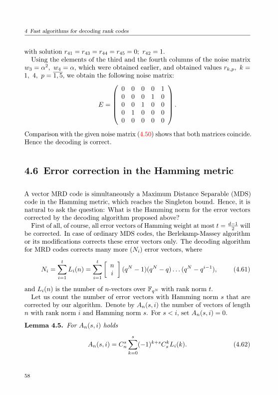
4 Fast algorithms for decoding rank codes
with solution r41 = r43 = r44 = r45 = 0; r42 = 1.Using the elements of the third and the fourth columns of the noise matrix
w3 = α2, w4 = α, which were obtained earlier, and obtained values rk,p, k =1, 4, p = 1, 5, we obtain the following noise matrix:
E =
0 0 0 0 10 0 0 1 00 0 1 0 00 1 0 0 00 0 0 0 0
.
Comparison with the given noise matrix (4.50) shows that both matrices coincide.Hence the decoding is correct.
4.6 Error correction in the Hamming metric
A vector MRD code is simultaneously a Maximum Distance Separable (MDS)code in the Hamming metric, which reaches the Singleton bound. Hence, it isnatural to ask the question: What is the Hamming norm for the error vectorscorrected by the decoding algorithm proposed above?
First of all, of course, all error vectors of Hamming weight at most t = d−12 will
be corrected. In case of ordinary MDS codes, the Berlekamp-Massey algorithmor its modifications corrects these error vectors only. The decoding algorithmfor MRD codes corrects many more (Ni) error vectors, where
Ni =
t∑i=1
Li(n) =
t∑i=1
[ni
](qN − 1)(qN − q) . . . (qN − qi−1), (4.61)
and Li(n) is the number of n-vectors over FqN with rank norm t.Let us count the number of error vectors with Hamming norm s that are
corrected by our algorithm. Denote by An(s, i) the number of vectors of lengthn with rank norm i and Hamming norm s. For s < i, set An(s, i) = 0.
Lemma 4.5. For An(s, i) holds
An(s, i) = Csn
s∑k=0
(−1)k+sCksLi(k). (4.62)
58
4 Fast algorithms for decoding rank codes
Indeed, An(s, i) = CsnAs(s, i). In addition, for all i ≤ s ≤ ns∑i=1
An(s, i) =
n∑s=i
CsnAs(s, i) = Li(n). (4.63)
By inverting the system (4.63) we obtain (4.62).From Lemma 4.5 follows
Theorem 4.6. The proposed above decoding algorithm for MRD codes corrects
Ms =
s∑i=1
An(s, i) = Csn
t∑i=1
s∑k=i
(−1)k+sCksLi(k), s = 1, 2, . . . , n, (4.64)
error vectors of Hamming norm s.
It can be shown that for s ≤ t holds: Ms = Csn(qN − 1)s .As an illustration consider codes over F2N with n = N and d = 3. In this
case t = 1 and according to (4.61) the total number of correctable error vectorsis N1 = (2N − 1)2. Out of this number, M1 = C1
N (2N − 1) error vectors haveHamming norm 1 and M2 = C2
N (2N − 1) vectors have Hamming norm 2, i.e.,double errors. The fraction of correctable double errors is 1
(2N−1). The norm of
other correctable errors is at least 3.A slight modification of the decoding algorithm allows us also to interpret
these error vectors as double errors. Assume that our decoding algorithmoutputs the error vector (E,E, . . . , E, 0, . . . , 0), with rank norm 1 and withHamming norm s ≥ 3. Let us solve the system
Xh1 + Y h2 = E(h1 + h2 + . . .+ hs),
Xh[1]1 + Y h
[1]2 = E(h
[1]1 + h
[1]2 + . . .+ h
[1]s ),
(4.65)
where h1, h2, . . . , hN are the elements of the first row of the check matrix. Thenthe vector (X,Y, 0, . . . , 0) has Hamming norm 2 and belongs to the same coset asthe vector (E,E, . . . , E, 0, . . . , 0). Thus, in the Hamming metric, the modifiedalgorithm gets closer to the full decoding algorithm. The full algorithm corrects22N − 1 error vectors of Hamming norms 1 and 2. The modified algorithmcorrects only (2N − 1)2 error vectors of norms 1 and 2, i.e., it does not correct2N+1 − 2 double errors in comparison with the full algorithm.
Similar modifications are possible for codes with a larger distance as well,however the complexity of the additional part of the algorithm grows fast withthe Hamming norm of correctable errors.
59


5Symmetric rank codes
5.1 Introduction
Rank metric codes can be described using either the matrix or the vector form.We recall it here again since we are going to introduce a new class of rank metriccodes called symmetric rank codes.
Let Fq be a field consisting of q elements and Fqn be its extension of order n.In this chapter we consider square code matrices only.To obtain the matrix description consider a normed ring Mn(Fq) of n × n
square matrices over the base field Fq. The norm of a matrix G is its rank,rank(G), and the rank distance d(G1, G2) between matrices G1, G2 is the rank oftheir difference, d(G1, G2) = rank(G1−G2). Any subsetM⊆Mn(Fq) is calleda code. The code distance d(M) = d is the minimum pairwise distance betweencode matrices, d = minrank(G1 − G2) : G1, G2 ∈ M;G1 6= G2. A code iscalled Fq-linear, if any linear combination of code matrices with coefficientsfrom Fq also belongs to the code. The code obtained by transposing matricesofM is called the transposed code MT . The codesM andMT have the samenumber of code matrices and the same code distance. IfM is Fq-linear thenMT is Fq-linear as well.
To get the vector description consider the normed space Fnqn of n-vectors overthe extension field Fqn . The norm or the rank of a vector g is the maximumnumber r(g) of its components that are linearly independent over the base field
61

5 Symmetric rank codes
Fq. The rank distance d(g1,g2) between vectors g1,g2 is the norm of theirdifference, d(g1,g2) = r(g1 − g2). A code V ⊆ Fnqn is a subset of vectors Fnqn .The code distance d(V) = d is the minimum pairwise distance between codevectors, d = minr(g1 − g2) : g1,g2 ∈ V; g1 6= g2. The code V is Fq-linear ifany linear combination of code vectors with coefficients from Fq also belongs tothe code. The code V is Fqn-linear if any linear combination of code vectorswith coefficients from Fqn also belongs to the code, i.e., if V is a linear subspaceof the space Fnqn . Fq-linearity follows from Fqn-linearity, however, the inversestatement is not true. For k = 1, 2, . . . , n there are known Fqn linear (n, k, d)-codes with maximum possible rank distance (MRD) d = n− k+ 1. These codesare k-dimensional subspaces of the space Fnqn .Let Ω = ω1, ω2, . . . , ωn be a basis of the extension field Fqn over the base
field Fq. Let θ−1 : Fqn ⇒ Fnq be the isomorphism from the field Fqn to the space
of column n-vectors over Fq. Elements of the basis are transformed to the linearindependent columns b1,b2, . . . ,bn ∈ Fnq , where bj = θ−1(ωj), j = 1, 2, . . . , n.
Let θ : Fnq ⇒ Fqn be the inverse transform θ(b) = β. Applying it to eachcolumn of the matrixM ∈Mn(Fq) we obtain one to one mapping Θ : Mn(Fq)⇒Kn
n of the space of (n× n)-matrices over Fq to the space of n-vectors over Fqn .Obviously, the rank of matrix M after the transform Θ(M) = g coincides withthe rank of the vector g, i.e., rank(M) = r(g).
The transform Θ is isometric. Given a matrix codeM the transform allowsus to get the vector code using V = Θ(M). And vice versa, given a vector codeV, we get the matrix codeM = Θ−1(V) with the same distance properties.
Vector form is more convenient to describe rank metric codes and fast decodingalgorithms. Matrix form is useful in the systems with coded modulation, e.g.in the theory of space-time codes.Using a known rank metric code one can design a new code with the same
cardinality and code distance as follows. Given a code V in vector form, twotransforms θ and θ, and also connected with them transforms Θ and Θ. Weobtain a new code VT using the following chain of transforms
V Θ−1
−→M −→MT Θ−→ VT . (5.1)
The code VT we call the transposed code in vector form. Note that transformsθ and θ may be different.The code VT has the same volume and the same rank-weight distribution
as the code V. However, if the code V is Fqn-linear (e.g. an MRD (n,k,d=n-k+1)-code), then the code VT is not necessarily Fqn -linear, despite it remaining
62

5 Symmetric rank codes
Fq-linear. This is a drawback of the construction, since fast decoding meth-ods for such codes are not known. One can decode the corrupted code vec-tor y = w + e, w ∈ VT , transforming it using (5.1) to the corrupted vectorz = v + e, v ∈ V, and use a standard method for decoding V. However, inthis case the question arises: Why should we use the code VT at all? Anotherdisadvantage of Fq-linear codes is an increase in the size of a generator matrixin comparison with Fqm-linear codes.Let us demonstrate this with the following example.Example 1. Let q = 2. For the code V we take the following one dimensional
Fqn-linear (n, 1, n)-code, n = 3.
V =(0, 0, 0), (1, α, α2), (α, α2, α3), (α2, α3, α4),(α3, α4, α5), (α4, α5, α6), (α5, α6, 1), (α6, 1, α),
where α is a root of the primitive polynomial f(λ) = λ3 +λ2 + 1. The generatormatrix of the code consists of a single row G = (1, α, α2), u = (u), u ∈ F23 , is anone dimensional information vector, the code vectors are v = uG = (u, uα, uα2).Let θ−1 be defined by 0 ↔ (0, 0, 0)T , 1 ↔ (1, 0, 0)T , α ↔ (0, 1, 0)T , α2 ↔
(0, 0, 1)T . Then the codeM is the following set of (3× 3)-matrices:
M0 =
0 0 00 0 00 0 0
,M1 =
1 0 00 1 00 0 1
,M2 =
0 0 11 0 00 1 1
,M3 =
0 1 10 0 11 1 1
,
M4 =
1 1 10 1 11 1 0
,M5 =
1 1 01 1 11 0 1
,M6 =
1 0 11 1 00 1 0
,M7 =
0 1 01 0 11 0 0
.The transposed code in vector form using θ is
VT =(0, 0, 0), (1, α, α2), (α2, 1, α6), (α6, α2, α4),(α4, α6, α3), (α5, α4, α3), (α3, α5, α), (α, α3, 1).
The code VT is Fq-linear, but it is not a linear space, i.e., it is not Fqn-linear.A generator matrix of the code is
G =
1 α α2
α2 1 α6
α6 α2 α4
,
63

5 Symmetric rank codes
an information vector is u = (u1, u2, u3), u1, u2, u3 ∈ F2. Code vectors arew = uG = (u1 + u2α
2 + u3α6, u1α+ u2 + u3α
2, u1α2 + u2α
6 + u3α4).
The finite field Fqn can be described in terms of (n× n)-matrices A over thefield Fq such that powers Ai, i = 1, 2, . . . , qn − 1, correspond to all nonzeroelements of Fqn . In this chapter, we will show that for fields Fqn of characteristic2 one can select a symmetric matrix A. We will show constructions of symmetricmatrices representing a field. Together with all-zero matrix these matrices forma Fqn-linear code with maximum distance d = n and with maximum possiblevolume qn for this distance. These codes are called symmetric rank codes. Invector form, they are MRD (n, 1, n)-codes with maximum rank distance andcan be decoded using known methods of error correction in rank metric. Forthe symmetric codes, we will suggest a method for erasure symmetrization thatallows for decreasing decoding complexity substantially in comparison withstandard approaches.
We will also show that a linear (n, k, d = n − k + 1) MRD code Vk thatincludes the previously mentioned one-dimensional symmetric code as a subcodehas the following property: corresponding transposed code is Fqn-linear. Suchcodes have increased capability to correct symmetric errors and erasures.
Given a linear (n, k, d = n− k + 1) MRD code V in vector form, can we findtransforms Θ and Θ (if they exist) such that the transposed code VT in vectorform is also a linear (n, k, d = n− k + 1) MRD code?
A positive answer will be given for a special case (n, 1, d = n) MRD codesand for fields Fqn of characteristic 2, i.e., q = 2r. From(5.1) it is easy to see:if the set M consists of symmetric matrices, then M = MT and for Θ = Θwe obtain V = VT . A linear (n, 1, d = n) MRD code V can be defined by asingle-row generator matrix
G = (g1, g2, . . . , gn),
where elements gj ∈ Fqn , j = 1, 2, . . . , n, are linearly independent over Fq.In this case, the code consists of the all zero vector 0 and vectors αsG, s =0, 1, . . . , qn − 2. We will show that there exist a single-row matrix G and atransform Θ such that Θ−1(αsG) = As, where A is a symmetric matrix.
64

5 Symmetric rank codes
5.2 Matrix and vector representations of exten-sion finite fields
Let A ∈Mn(Fq).
Definition 2. A matrix A represents the field Fqn if the algebra of polynomialsFq[A] is isomorphic to Fqn .
We say that the matrix A gives a primitive representation of the field if allmatrices As, s = 1, 2, . . . , qn − 1, are different. The following lemma gives acharacterization of such matrices.
Lemma 5.1. A matrix A ∈ Mn(Fq) gives a primitive representation of thefield Fqn if and only if its characteristic polynomial det(λIn −A) is a primitivepolynomial f(λ) over Fq of degree n,
f(λ) = λn + fn−1λn−1 + fn−3λ
n−2 + . . .+ f1λ1 + f0. (5.2)
Recall the definition: A non-reducible over Fq polynomial f(λ) of degree n iscalled primitive if f(λ) divides the binomial λq
n−1 − 1, but does not divide thebinomials λs − 1, 1 ≤ s ≤ qn − 2.
Proof. Let det(λIn − A) = f(λ), where f(λ) is primitive. Then f(A) = On,where On is the n × n all zero matrix. Since the polynomial f(λ) dividesλq
n−1 − 1, but does not divide the binomials λs − 1, 1 ≤ s ≤ qn − 2, wehave Aq
n−1 = In, and all the matrices As, s = 1, 2, . . . , qn − 1, are different.Moreover, all the matrices As can be written as linear combinations of matricesIn, A,A
2, . . . , An−1 using An = −fn−1An−1 − fn−2A
n−2 − . . . − f1A − f0In.Hence, the algebra of matrix polynomials Fqn [A] is isomorphic to the field Fqnobtained by joining a root α of the primitive polynomial f(λ) to the field Fq.Thus, the matrix A gives primitive representation of the field Fqn .
The inverse is also true. Let the matrix A give primitive representation ofthe field Fqn . Then the minimal polynomials of A and α are the same and theycoincide with a primitive polynomial f(λ). Since the characteristic polynomialis divisible by the minimal polynomial and has the same degree and the sameleading coefficient, we get det(λIn −A) = f(λ).
65

5 Symmetric rank codes
Corollary 5.2. All the matrices A that represent the field Fqn are similar tothe matrix
C =
0 0 . . . 0 −f0
1 0 . . . 0 −f1
· · · · · · ·0 0 . . . 0 −fn−2
0 0 . . . 1 −fn−1
,
i.e., A = QCQ−1, where Q ∈Mn(Fq) is a nonsingular matrix and f0, f1, . . . , fn−1
are coefficients of a monic primitive polynomial
f(λ) = λn + fn−1λn−1 + fn−3λ
n−2 + . . .+ f1λ1 + f0.
Proof. Characteristic polynomials of similar matrices coincide. We havedet(λIn −C) = λn + fn−1λ
n−1 + fn−2λn−2 + . . .+ f1λ
1 + f0 = f(λ). Let A bean n× n matrix with a characteristic polynomial det(λIn −A) = f(λ). Sincef(λ) is primitive, the sets of invariant polynomials of the matrices λIn − Aand λIn − C are the same: f(λ), 1, . . . , 1. Hence, according to the necessaryand sufficient condition [Gan67], the matrix A is similar to the matrix C, i.e.,A = QCQ−1, where Q is a non-singular matrix over the base field Fq.
LetM [j] denote the j−th column of a matrixM. Let A be a matrix that givesprimitive representation of the field Fqn . Define induced vector representationof the field Fqn as follows
θ−1(0) = On[1],θ−1(αs) = As[1],
θ(On[1]) = 0,θ(As[1]) = αs, s = 0, 1, . . . , qn − 2.
. (5.3)
We say that this representation is agreed with the matrix A.
Lemma 5.3. Let c ∈ Fqn then
θ−1(αc) = Aθ−1(c),
where α is a primitive element of Fqn .
Proof. Since c = αs for some s, then θ−1(αc) = θ−1(α1+s) = A1+s[1] =AAs[1] = Aθ−1(c).
Recall: given a vector c = (c1, c2, . . . , cn) ∈ Fqn , we define
Θ−1(c) = (θ−1(c1), θ−1(c2), . . . , θ−1(cn)). (5.4)
66
5 Symmetric rank codes
Thus, Θ−1(c) = M is an (n× n)-matrix over the field Fq.Clearly
Θ−1(αc) = AΘ−1(c) = AM,
and in general case
Θ−1(αsc) = AsΘ−1(c) = AsM, s = 1, 2, . . . . (5.5)
The inverse also holds:
Θ(AsM) = αsΘ(M) = αsc.
In addition, if c ∈ Fqn and R is an (n×m)-matrix over the field Fq, then
Θ−1(cR) = Θ−1(c)R = MR.
5.3 Symmetric matrices representing a field
Let us show that the matrix A representing the field Fqn , q = 2n, of characteristic2 can be selected to be symmetric1. The first such construction was suggestedin [GP02] for fields of characteristic 2, and it uses 2n− 1 free parameters. Herewe describe a simpler construction with n free parameters only [GP04, GP06].
5.3.1 Auxiliary matrices and determinants
All operations are in a field F of characteristic 2.Let Dn(λ) be the tridiagonal λ−matrix of order n, with λ on the main
1Examples show that for n = 2, 3 one can find symmetric matrices representing the field of
arbitrary characteristic p. For example, the matrix A =
(1 11 0
)represents the field F32 .
However, a general construction is not known. The fields of characteristic 0 cannot berepresented by symmetric matrices.
67

5 Symmetric rank codes
diagonal and 1 in the neighboring positions
Dn(λ) =
λ 1 0 . . . 0 0 01 λ 1 . . . 0 0 00 1 λ . . . 0 0 0...
......
. . ....
......
0 0 0 . . . λ 1 00 0 0 . . . 1 λ 10 0 0 . . . 0 1 λ
. (5.6)
The determinant of this matrix is denoted by dn(λ).Let Hn(λ) be the tridiagonal λ−matrix of order n, where the last element of
the main diagonal is λ+ 1:
Hn(λ) =
λ 1 0 . . . 0 0 01 λ 1 . . . 0 0 00 1 λ . . . 0 0 0...
......
. . ....
......
0 0 0 . . . λ 1 00 0 0 . . . 1 λ 10 0 0 . . . 0 1 λ+ 1
. (5.7)
Denote the determinant of this matrix by hn(λ). Let us define d−1(λ) =0, d0(λ) = 1, h−1(λ) = 1, h0(λ) = 1. It is easy to see that d1(λ) = λ, h1(λ) =λ+ 1.
The determinants dn(λ) and hn(λ) can be computed recurrently
dn(λ) = d1(λ)dn−1(λ) + dn−2(λ), n ≥ 2;hn(λ) = d1(λ)hn−1(λ) + hn−2(λ), n ≥ 2.
(5.8)
Further, using (5.8) repeatedly, we get for s ≥ 1
dn(λ) = ds(λ)dn−s(λ) + ds−1(λ)dn−s−1(λ), n ≥ 2;hn(λ) = ds(λ)hn−s(λ) + ds−1(λ)hn−s−1(λ), n ≥ 2.
(5.9)
5.3.2 The main construction
In fields of characteristic 2, every element is a square of another. Selectthe elements an−1, an−2 = b2n−2, an−3 = b2n−3, . . . , a0 = b20 ∈ F. Let b =
68

5 Symmetric rank codes
(bn−2, bn−3, . . . , b0). Consider the following bordered symmetric matrix:
A =
(an−1 bbT Hn−1(0)
)=
an−1 bn−2 bn−3 bn−4 . . . b2 b1 b0bn−2 0 1 0 . . . 0 0 0bn−3 1 0 1 . . . 0 0 0bn−4 0 1 0 . . . 0 0 0...
......
.... . .
......
...b2 0 0 0 . . . 0 1 0b1 0 0 0 . . . 1 0 1b0 0 0 0 . . . 0 1 1
.
(5.10)Let
g(λ) = λn + gn−1λn−1 + gn−3λ
n−2 + . . .+ g1λ1 + g0 (5.11)
be an arbitrary monic polynomial of degree n over F.
Theorem 5.4. There exists a matrix (5.10) with a characteristic polynomialg(λ).
Proof. Let us compute the characteristic polynomial of A
χn(λ) = det(λIn +A) = det
(λ+ an−1 b
bT Hn−1(λ)
)
= det
λ+ an−1 bn−2 bn−3 bn−4 . . . b2 b1 b0bn−2 λ 1 0 . . . 0 0 0bn−3 1 λ 1 . . . 0 0 0bn−4 0 1 λ . . . 0 0 0...
......
.... . .
......
...b2 0 0 0 . . . λ 1 0b1 0 0 0 . . . 1 λ 1b0 0 0 0 . . . 0 1 λ+ 1
.
(5.12)
By decomposing the determinant using elements of the first row, and thendecomposing the determinants obtained using elements of the first column, after
69

5 Symmetric rank codes
simplifications we obtain
χn(λ) = (λ+ an−1)hn−1(λ) + b2n−2hn−2(λ) + b2n−3d1(λ)hn−3(λ) + . . .+b21dn−3(λ)h1(λ) + b20dn−2(λ)= (λ+ an−1)hn−1(λ) + an−2hn−2(λ) + an−3d1(λ)hn−3(λ) + . . .+a1dn−3(λ)h1(λ) + a0dn−2(λ),
(5.13)where polynomials hi(λ) and di(λ) are defined by (5.8).
The relation (5.13) shows that the characteristic polynomial χn(λ) is a linearcombination of polynomials
(λhn−1(λ), hn−1(λ), hn−2(λ), d1(λ)hn−3(λ), . . . , dn−3(λ)h1(λ), dn−2(λ))(5.14)
with coefficients
(1, an−1, an−2, . . . , a1, a0). (5.15)
Let us show that the polynomials (5.14) are linearly independent over F. Thepolynomial λhn−1(λ) has degree n, the polynomial hn−1(λ) has degree n− 1,and the rest of the polynomials
(hn−2(λ), d1(λ)hn−3(λ), . . . , dn−3(λ)h1(λ), dn−2(λ)) (5.16)
have degree n−2. It is sufficient to show the linear independency of polynomials(5.16). Let us add the polynomial hn−2(λ) in the system (5.16) to all the otherpolynomials ds(λ)hn−2−s(λ), s = 1, 2, . . . , n− 2. Using (5.9), we get hn−2(λ) +ds(λ)hn−2−s(λ) = ds−1(λ)hn−3−s(λ), where the degrees of polynomialsds−1(λ)hn−3−s(λ) are n− 4. As a result, the system of polynomials (5.16) istransformed to the system
(hn−2(λ), hn−4(λ), d1(λ)hn−5(λ), . . . , dn−5(λ)h1(λ), dn−4(λ), dn−3(λ)).(5.17)
The first polynomial hn−2(λ) of the system has degree n − 2, the last one,dn−3(λ), has degree n− 3, the remaining polynomials
(hn−4(λ), d1(λ)hn−5(λ), . . . , dn−5(λ)h1(λ), dn−4(λ))
have degree n− 4 and are similar to (5.16). By iterative continuation of this
70
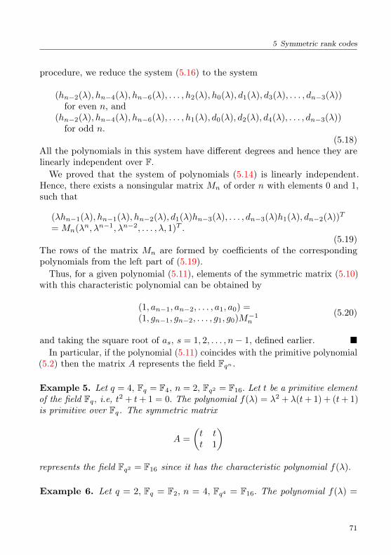
5 Symmetric rank codes
procedure, we reduce the system (5.16) to the system
(hn−2(λ), hn−4(λ), hn−6(λ), . . . , h2(λ), h0(λ), d1(λ), d3(λ), . . . , dn−3(λ))for even n, and
(hn−2(λ), hn−4(λ), hn−6(λ), . . . , h1(λ), d0(λ), d2(λ), d4(λ), . . . , dn−3(λ))for odd n.
(5.18)All the polynomials in this system have different degrees and hence they arelinearly independent over F.We proved that the system of polynomials (5.14) is linearly independent.
Hence, there exists a nonsingular matrix Mn of order n with elements 0 and 1,such that
(λhn−1(λ), hn−1(λ), hn−2(λ), d1(λ)hn−3(λ), . . . , dn−3(λ)h1(λ), dn−2(λ))T
= Mn(λn, λn−1, λn−2, . . . , λ, 1)T .(5.19)
The rows of the matrix Mn are formed by coefficients of the correspondingpolynomials from the left part of (5.19).
Thus, for a given polynomial (5.11), elements of the symmetric matrix (5.10)with this characteristic polynomial can be obtained by
(1, an−1, an−2, . . . , a1, a0) =(1, gn−1, gn−2, . . . , g1, g0)M−1
n(5.20)
and taking the square root of as, s = 1, 2, . . . , n− 1, defined earlier. In particular, if the polynomial (5.11) coincides with the primitive polynomial
(5.2) then the matrix A represents the field Fqn .
Example 5. Let q = 4, Fq = F4, n = 2, Fq2 = F16. Let t be a primitive elementof the field Fq, i.e, t2 + t+ 1 = 0. The polynomial f(λ) = λ2 + λ(t+ 1) + (t+ 1)is primitive over Fq. The symmetric matrix
A =
(t tt 1
)represents the field Fq2 = F16 since it has the characteristic polynomial f(λ).
Example 6. Let q = 2, Fq = F2, n = 4, Fq4 = F16. The polynomial f(λ) =
71
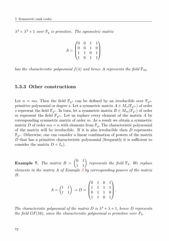
5 Symmetric rank codes
λ4 + λ3 + 1 over Fq is primitive. The symmetric matrix
A =
0 0 1 10 0 1 01 1 0 11 0 1 1
has the characteristic polynomial f(λ) and hence A represents the field F16.
5.3.3 Other constructions
Let n = ms. Then the field Fqn can be defined by an irreducible over Fqmprimitive polynomial or degree s. Let a symmetric matrix A ∈Ms(Fqm) of orders represent the field Fqn . In turn, let a symmetric matrix B ∈Mm(Fqs) of orderm represent the field Fqm . Let us replace every element of the matrix A bycorresponding symmetric matrix of order m. As a result we obtain a symmetricmatrix D of order ms = n with elements from Fq. The characteristic polynomialof the matrix will be irreducible. If it is also irreducible then D representsFqn . Otherwise, one can consider a linear combination of powers of the matrixD that has a primitive characteristic polynomial (frequently it is sufficient toconsider the matrix D + In).
Example 7. The matrix B =
(0 11 1
)represents the field F4. We replace
elements in the matrix A of Example 5 by corresponding powers of the matrixB:
A =
(t tt 1
)→ D =
0 1 0 11 1 1 10 1 1 01 1 0 1
.
The characteristic polynomial of the matrix D is λ4 + λ+ 1, hence D representsthe field GF (16), since the characteristic polynomial is primitive over F2.
72
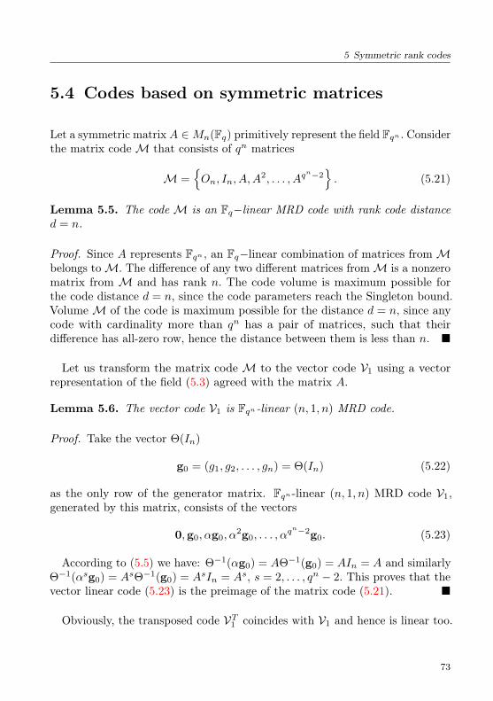
5 Symmetric rank codes
5.4 Codes based on symmetric matrices
Let a symmetric matrix A ∈Mn(Fq) primitively represent the field Fqn . Considerthe matrix codeM that consists of qn matrices
M =On, In, A,A
2, . . . , Aqn−2. (5.21)
Lemma 5.5. The codeM is an Fq−linear MRD code with rank code distanced = n.
Proof. Since A represents Fqn , an Fq−linear combination of matrices fromMbelongs toM. The difference of any two different matrices fromM is a nonzeromatrix from M and has rank n. The code volume is maximum possible forthe code distance d = n, since the code parameters reach the Singleton bound.VolumeM of the code is maximum possible for the distance d = n, since anycode with cardinality more than qn has a pair of matrices, such that theirdifference has all-zero row, hence the distance between them is less than n.
Let us transform the matrix code M to the vector code V1 using a vectorrepresentation of the field (5.3) agreed with the matrix A.
Lemma 5.6. The vector code V1 is Fqn-linear (n, 1, n) MRD code.
Proof. Take the vector Θ(In)
g0 = (g1, g2, . . . , gn) = Θ(In) (5.22)
as the only row of the generator matrix. Fqn-linear (n, 1, n) MRD code V1,generated by this matrix, consists of the vectors
0,g0, αg0, α2g0, . . . , α
qn−2g0. (5.23)
According to (5.5) we have: Θ−1(αg0) = AΘ−1(g0) = AIn = A and similarlyΘ−1(αsg0) = AsΘ−1(g0) = AsIn = As, s = 2, . . . , qn − 2. This proves that thevector linear code (5.23) is the preimage of the matrix code (5.21).
Obviously, the transposed code VT1 coincides with V1 and hence is linear too.
73

5 Symmetric rank codes
5.5 Erasure correction
It is appropriate to explain rank erasures for the matrix form of a code. Forgeneral MRD codes joint error and erasure correction was considered in Chapter4.
In applications, a code vector should be converted to a matrix form, andevery element of the matrix is transmitted over a channel. The receiver makes ahard decision about every element. Only after this, is the matrix converted to avector to be used by an algebraic decoder. The received matrix is Y = M + E,where M is a code matrix and E is an error matrix, which will also be calleda rank error. If rank(E) ≤ (d− 1)/2, then the algebraic decoder corrects thiserror.
Sometimes, while making the hard decision the unreliability of every symbolcan be estimated. Then the matrix of unreliabilities Z can be used for decodingtogether with the matrix Y . An element zij of the matrix Z shows the unrelia-bility of the element yij of the matrix Y . We consider an idealized case wherethe matrix Z consists of zeroes and ones only. The value zij = 0 shows that thedecision about yij is correct. The value zij = 1 means that the decision aboutyij can be wrong. In this case, we assume that the symbol was erased, despite,in fact, some decision about the symbol having been made. In this case, we callthe matrix E rank erasure. The decoder obtains the matrix Y and the matrixZ of reliabilities, and hence it knows the error free positions. The matrix E haszeros at these positions, known to the decoder. We say that such a matrix E isagreed with the matrix of unreliabilities Z.
The rank of erasure is the rank of the matrix E. Consider all the matrices Eagreed with the matrix Z. Let rmax(Z) denote the maximum possible rank ofthe matrix E. Obviously, a code with rank distance d corrects rank erasure Eagreed with the matrix Z if rmax(Z) ≤ d− 1.
To estimate rmax(Z) it is convenient to use the concept of the term rank of amatrix from combinatorics.The term rank of a matrix A, denoted by termrank(A), is the maximum
number t of nonzero elements in the matrix such that no two of them belong toone line (row or column).
Lemma 5.7. The term rank of a (0, 1)-matrix Z is the minimum number t oflines (rows and columns) that contain all nonzero elements of the matrix Z.
Using this lemma we obtain
74

5 Symmetric rank codes
Lemma 5.8. rmax(Z) = termrank(Z).
Proof. We have rank(E) ≤ termrank(E). For any matrix E, agreed with thematrix Z, it holds that termrank(E) ≤ termrank(Z). Hence, on the one handit follows that
rmax(Z) ≤ termrank(Z).
On the other hand, let termrank(Z) = t. Then there are t positions withnonzero elements in Z such that no two of them belong to one line. Take amatrix E agreed with Z that has nonzero elements at these positions and zeroselsewhere. The rank of E is t, hence
rmax(Z) ≥ termrank(Z)
and the statement of the lemma follows.
Consider erasure correction using the code V1, defined by (5.21) and (5.22).Denote [j] = qj if j ≥ 0 and [j] = qn+j if j < 0. The expression g[j] = gq
j
is called j-th Frobenius power of the element g. In particular, g[n] = gqn
= g.Frobenius power of a vector is computed componentwise.For decoding we will use the following check matrix Hn−1 = (h
[i]j ), i =
0, 1, . . . , n− 2, j = 1, 2, . . . , n, such that g0HTn−1 = 0.
Let y = αsG+e be the received signal in vector form where e = (e1, e2, . . . , en)denotes the vector form of the rank erasure E. Calculation of the syndromegives the system of n− 1 equations over the field Fqn :
n∑j=1
ejh[i]j = si, i = 0, 1, . . . , n− 2.
Since the positions of possible errors in the matrix E are known, the systemcan be rewritten as a system with n(n− 1) linear equations over the base field,considering possible errors as unknowns. The number of unknowns depends onthe configuration of the matrix E. If the rank of erasure is n− 1 and errors arein n− 1 rows or in n− 1 columns, then the number of unknowns is maximaland equals n(n− 1). In this case the complexity to obtain a solution is maximal.If the rank of erasure is n− 1 and errors are in bn/2c rows and in b(n− 1)/2ccolumns, then the number of unknowns s is s = n(n− 1)− bn/2cb(n− 1)/2c,i.e., it is decreased by approximately a quarter. Thus, the syndrome decoding
75

5 Symmetric rank codes
of erasures can be reduced to solving a system of n(n − 1) linear equationswith n(n − 1) unknowns at most. The complexity decreases with decreasingthe number of unknowns.In the case of symmetric rank codes, the number of unknowns can be sub-
stantially decreased using a trick that we call symmetrization of rank erasuresLet Y = M +E be a received signal in matrix form and E be a rank erasure.
Additional information about errors can be obtained by computing the matrixQ = Y +Y T = M+MT+E+ET . Since for symmetric codesM = MT , M ∈M,we have for fields of characteristic 2: M +MT = On, therefore we know
Q = Y + Y T = E + ET .
The matrix of unreliabilities Z shows the positions of zeroes in the matrixE. This allows us, during analysis of the matrix E + ET , to obtain part of theerrors directly and obtain additional information for another part.Let us show the possible situations by the following example.Example 5. Let n = 4, d = 4 and let the matrix of unreliabilities be
Z =
1 1 1 11 1 1 10 0 0 10 0 0 1
.
This means that the matrix of errors is
E =
a1 a2 a3 a4
a5 a6 a7 a8
0 0 0 a9
0 0 0 a10
,
and it has the rank d − 1 = 3 at most. In total, the matrix has ten binaryunknowns ai at known positions. Then we have
Q = E + ET =
0 a2 + a5 a3 a4
a5 + a2 0 a7 a8
a3 a7 0 a9
a4 a8 a9 0
.
From this matrix, we immediately obtain the error values a3, a4, a7, a8, a9. Wealso know the sum a2 + a5 = b. However, the matrix Q has no informationabout “diagonal” errors a1, a6, a10.
76

5 Symmetric rank codes
Let us modify the received matrix Y by adding the upper triangular knownmatrix
R =
0 b a3 a4
0 0 a7 a8
0 0 0 a9
0 0 0 0
.
We obtain
Ymod = Y +R = M + E +R = M + Emod,
where
Emod =
a1 a5 0 0a5 a6 0 00 0 0 00 0 0 a10
is a symmetric error matrix, which has only four unknown error values at knownpositions. We call this procedure symmetrization of erasures.The matrix Ymod can be decoded using the syndrome correction of erasures.
The preliminary symmetrization decreased the number of unknowns from 10 to4.
Remark. In the class of codes under consideration, any line (row or column)of a code matrix is an information set. If for every known line we precomputethe rest of the code matrix, then the decoding can be simplified when one oflines in the received matrix is error free. In Example 5, after symmetrizationwe have the error matrix that has zero lines (the third row or column), hencethe syndrome decoding can be avoided.In the general case, the symmetrization decreases the number of unknowns
by at least half. For the case where erasure rank is d− 1 = n− 1 and all errorsare in n − 1 rows, the symmetrization decreases the number of unknowns ton(n− 1)/2 in comparison with n(n− 1) without symmetrization.Let n = 2s + 1. If the erasure rank is n − 1 and the errors are in the first
s rows and the last s columns then after the symmetrization the number ofunknowns decreases from (3n2−2n−1)
4 to (n2−1)4 , i.e., making it approximately
three times smaller.
77
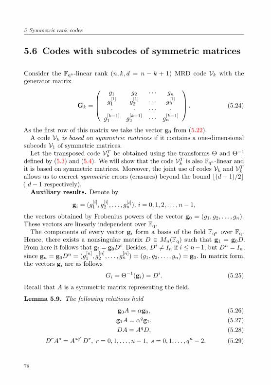
5 Symmetric rank codes
5.6 Codes with subcodes of symmetric matrices
Consider the Fqn-linear rank (n, k, d = n − k + 1) MRD code Vk with thegenerator matrix
Gk =
g1 g2 · · · gn
g[1]1 g
[1]2 · · · g
[1]n
· · · · · ·g
[k−1]1 g
[k−1]2 · · · g
[k−1]n
. (5.24)
As the first row of this matrix we take the vector g0 from (5.22).A code Vk is based on symmetric matrices if it contains a one-dimensional
subcode V1 of symmetric matrices.Let the transposed code VTk be obtained using the transforms Θ and Θ−1
defined by (5.3) and (5.4). We will show that the code VTk is also Fqn -linear andit is based on symmetric matrices. Moreover, the joint use of codes Vk and VTkallows us to correct symmetric errors (erasures) beyond the bound b(d− 1)/2c( d− 1 respectively).Auxiliary results. Denote by
gi = (g[i]1 , g
[i]2 , . . . , g
[i]n ), i = 0, 1, 2, . . . , n− 1,
the vectors obtained by Frobenius powers of the vector g0 = (g1, g2, . . . , gn).These vectors are linearly independent over Fq.
The components of every vector gi form a basis of the field Fqn over Fq.Hence, there exists a nonsingular matrix D ∈ Mn(Fq) such that g1 = g0D.From here it follows that gi = g0D
i. Besides, Di 6= In if i ≤ n−1, but Dn = In,since gn = g0D
n = (g[n]1 , g
[n]2 , . . . , g
[n]n ) = (g1, g2, . . . , gn) = g0. In matrix form,
the vectors gi are as follows
Gi = Θ−1(gi) = Di. (5.25)
Recall that A is a symmetric matrix representing the field.
Lemma 5.9. The following relations hold
g0A = αg0, (5.26)g1A = αqg1, (5.27)DA = AqD, (5.28)
DrAs = Asqr
Dr, r = 0, 1, . . . , n− 1, s = 0, 1, . . . , qn − 2. (5.29)
78

5 Symmetric rank codes
Proof. To prove (5.26) we apply to its both parts the transform Θ−1:Θ−1(g0A) = Θ−1(g0)A = InA = A. On the other hand according to (5.5) weobtain Θ−1(αg0) = AΘ−1(g0) = AIn = A.
The relation (5.27) follows from (5.26) if we raise both parts of (5.26) to thefirst Frobenius power and take into account that A ∈Mn(Fq). We obtain (5.28)if we apply the transform Θ to both parts of (5.27).The relation (5.29) follows from (5.28) if we separate factors DA in the left
part of (5.29) and use (5.28).
Lemma 5.10. The matrices D and DT are connected by the relation
DT = AmDn−1, (5.30)
where m is an integer.
Proof. Transpose matrices in (5.28) and take into account that A is a symmetricmatrix, then we obtain DTAq = ADT . Left multiply both parts of (5.28) bythe matrix DT and obtain DTDA = DTAqD = ADTD. It follows from herethat the matrix DTD commutes with the matrix A. Since all eigenvalues of thematrix A (in some field extension) are different, the matrix DTD can only be apolynomial in A and hence it is a power m of A [Gan67].
Matrix form of the code Vk. A generator matrix of the code Vk consists ofthe first k vectors gj , j = 0, 1, . . . , k−1.Write components of an information vec-tor u = (u0, u1, . . . , uk−1) as powers of α, i.e., u = (ε0α
s0 , ε1αs1 , . . . , εk−1α
sk−1).Here the coefficients εj equal zero if uj = 0 and equal 1 if uj 6= 0. Then thecode vector corresponding to the information vector u is
g(u) =
k−1∑j=0
εjαsjgj .
Let us convert this vector to the matrix M(u) using (5.5) and (5.25):
M(u) = Θ−1(g(u)) =
k−1∑j=0
εjAsjDj . (5.31)
The set of matricesM = M(u) from (5.31) for the all possible informationvectors u define the code Vk in matrix form.
79
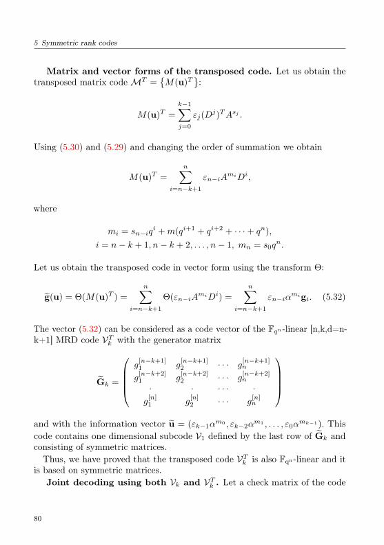
5 Symmetric rank codes
Matrix and vector forms of the transposed code. Let us obtain thetransposed matrix codeMT =
M(u)T
:
M(u)T =
k−1∑j=0
εj(Dj)TAsj .
Using (5.30) and (5.29) and changing the order of summation we obtain
M(u)T =
n∑i=n−k+1
εn−iAmiDi,
where
mi = sn−iqi +m(qi+1 + qi+2 + · · ·+ qn),
i = n− k + 1, n− k + 2, . . . , n− 1, mn = s0qn.
Let us obtain the transposed code in vector form using the transform Θ:
g(u) = Θ(M(u)T ) =
n∑i=n−k+1
Θ(εn−iAmiDi) =
n∑i=n−k+1
εn−iαmigi. (5.32)
The vector (5.32) can be considered as a code vector of the Fqn -linear [n,k,d=n-k+1] MRD code VTk with the generator matrix
Gk =
g
[n−k+1]1 g
[n−k+1]2 · · · g
[n−k+1]n
g[n−k+2]1 g
[n−k+2]2 · · · g
[n−k+2]n
· · · · · ·g
[n]1 g
[n]2 · · · g
[n]n
and with the information vector u = (εk−1α
m0 , εk−2αm1 , . . . , ε0α
mk−1). Thiscode contains one dimensional subcode V1 defined by the last row of Gk andconsisting of symmetric matrices.Thus, we have proved that the transposed code VTk is also Fqn-linear and it
is based on symmetric matrices.Joint decoding using both Vk and VTk . Let a check matrix of the code
80
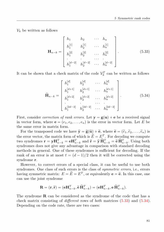
5 Symmetric rank codes
Vk be written as follows
Hn−k =
h1 h2 · · · hn
h[1]1 h
[1]2 · · · h
[1]n
h[2]1 h
[2]2 · · · h
[2]n
· · · · · ·h
[d−2]1 h
[d−2]2 · · · h
[d−2]n
. (5.33)
It can be shown that a check matrix of the code VTk can be written as follows
Hn−k =
h[d]1 h
[d]2 · · · h
[d]n
h[d+1]1 h
[d+1]2 · · · h
[d+1]n
h[d+2]1 h
[d+2]2 · · · h
[d+2]n
· · · · · ·h
[2d−2]1 h
[2d−2]2 · · · h
[2d−2]n
. (5.34)
First, consider correction of rank errors. Let y = g(u) + e be a received signalin vector form, where e = (e1, e2, . . . , en) is the error in vector form. Let E bethe same error in matrix form.For the transposed code we have y = g(u) + e, where e = (e1, e2, . . . , en) is
the error vector, the matrix form of which is E = ET . For decoding we computetwo syndromes r = yHT
n−k = eHTn−k and r = y HT
n−k = e HTn−k. Using both
syndromes does not give any advantage in comparison with standard decodingmethods in general. One of these syndromes is sufficient for decoding. If therank of an error is at most t = (d − 1)/2 then it will be corrected using thesyndrome r.However, to correct errors of a special class, it can be useful to use both
syndromes. One class of such errors is the class of symmetric errors, i.e., errorshaving symmetric matrix: E = E = ET , or equivalently e = e. In this case, onecan use the joint syndrome
R = (r, r) = (eHTn−k, e HT
n−k) = (eHTn−k, e HT
n−k).
The syndrome R can be considered as the syndrome of the code that has acheck matrix consisting of different rows of both matrices (5.33) and (5.34).Depending on the code rate, there are two cases:
81
5 Symmetric rank codes
1. Let 2d− 2 < n, i.e., R = k/n > 1/2. Then all rows of both matrices aredifferent. The corresponding code can have a distance up to D = 2d− 1,hence, symmetric errors of rank up to (D− 1)/2 = d− 1 can be correctedusing the syndrome R.
2. Let 2d− 2 ≥ n, i.e., R = k/n ≤ 1/2. Then the number of different rows inboth matrices is n− 1. The corresponding code has the distance D = n,and symmetric errors of rank up to (n− 1)/2 can be corrected using thesyndrome R.
Similar results hold for correction of symmetric rank erasures. If R = k/n >1/2 then for some codes, symmetric erasures of rank up to D − 1 = 2d− 2 canbe corrected using the syndrome R. If R = k/n ≤ 1/2 then symmetric erasuresof rank up to n− 1 can be corrected using the syndrome R.
5.7 Conclusions
We have shown that finite fields of characteristic 2 can be defined by symmetricmatrices, and we have presented a matrix code with maximum possible distanceand volume.
82

6Rank metric codes in network coding
6.1 Principles of network coding
Network coding is a relatively new research field. It is based on modification ofinformation flow in a ordinary network. Formally, a communication network canbe described as a finite directed graph, where vertices (nodes) can be connectedby more than one edge. A vertex without input edges is called a source node.
Consider the following model. A communication network consists of verticesconnected by communication channels (lines). Information is transmitted overeach channel without distortions with a rate up to the channel capacity. Datafrom a source vertex should be transmitted to a set of fixed destination nodes.The natural question is: Given the restrictions above on the communicationchannels, can this problem be solved and how can it be done efficiently?Existing computer networks transmit messages (packets) from a source to
destinations using a number of intermediate nodes working on the principle“receive and forward”. An intermediate node receives a packet from an input line,stores it in a buffer, and then sends copies of the packet via output lines thatcan deliver the packet to destinations possibly using other intermediate nodes.No other processing of packets at intermediate nodes is assumed. The optimalrouting problem should be solved for this traditional approach. A simple modelof a traditional network consists of one source, one destination, and a numberof intermediate nodes.
83

6 Rank metric codes in network coding
The concept “network coding” was introduced in 2000 [ANLY00]. The authorsconsider packets as vectors over finite fields and assume that intermediate nodescan compute linear combinations of received packets. In the new model, anintermediate node is responsible for the following operations:
• receive packets;
• store them in a buffer;
• compute linear combinations of received packets;
• send the linear combinations to a next node.
Transmission of linear combinations of packets makes it possible to increase thenetwork capacity: the maximum number of packets that can be transmitted to adestination per time unit. In the case of multiple destinations, the transmissiontime is the minimum time until all the destinations have received all thetransmitted packets. The authors of [ANLY00] were the first to show by anexample that network coding can increase the capacity of a network.The possibility of increasing network capacity aroused considerable interest
among researchers. In a number of publications, linear combinations of packetswere considered with both random and deterministic coefficients. It was shownthat the problems of network coding intersect with problems of error correctingcodes and with general information theory. The first publications assumed thatnetwork coding should depend on the known topology of a network. This wasnot convenient for both theory and practice.A new approach based on the subspace metric was suggested in 2007 by
Kötter and Kschischang [KK08]. Soon after this, Silva, a PhD student ofKschischang,joined the research team. In their research, Silva, Kötter, andKschischang [SKK08] considered linear combinations of packets with randomcoefficients. Such network coding was called random network coding. Later itwas also called non-coherent coding. Network coding with known coefficientswas called non-coherent. Silva, Kötter, and Kschischang show that problems ofsubspace coding can be reduced to problems of algebraic coding, such as design-ing codes in a given metric, obtaining bounds for optimal codes, constructingcoding and decoding algorithms. They used Gabidulin rank metric codes forerror correction in networks.
84
6 Rank metric codes in network coding
6.2 Spaces and subspaces
Before we describe subspace network codes let us recall main definitions con-nected with spaces and subspaces [Sag10].
6.2.1 Linear vector spaces
A linear vector space over the finite field Fq is a set of vectors V that satisfiesthe following conditions.
• The set V is an abelian additive group.
• For any γ ∈ Fq and v ∈ V it holds that γv ∈ V .
• Axioms of distributivity are satisfied: if γ ∈ Fq and v, u ∈ V , thenγ(u+ v) = γu+ γv; if γ, λ ∈ Fq and v ∈ V , then (γ + λ)v = γv + λv.
• Associativity of multiplication: (γλ)v = γ(λv).
Elements γ, λ ∈ Fq are called scalars.The maximum number of linearly independent vectors of a space is called its
dimension, and a set of such vectors is called a basis of the space.A subset of a space is called a subspace if this subset satisfies the conditions
of a space.Denote by WN,q a fixed N -dimensional vector space over the finite field Fq
and by P(WN,q) denote the set of all subspaces in WN,q.The dimension of an element V ∈ P(WN,q) is denoted by dim(V ). There are
subspaces of dimensions 0, 1, . . . , N . The subspace O of dimension 0 consistsof a single all zero N -vector. An m-dimensional subspace V consists of qmvectors of length N over the field Fq. It can be viewed as a row space of ann × N matrix M(V ) of rank m over Fq, where n ≥ m. The matrix M(V ) iscalled a generator matrix of m-dimensional subspace V and it is not unique.Let T be a nonsingular square matrix of order n over the field Fq, then therow space of the matrix TM(V ) coincides with the subspace V . Hence, thematrix TM(V ) is a generator matrix of the subspace V as well. Obviously, thedimension of the subspace and the rank of a generator matrix are equal, i.e.,dim(V ) = Rk(M(V )), where Rk(A) denotes the rank of matrix A. If n = m,then the matrix M(V ) is called a basic generator matrix.
85
6 Rank metric codes in network coding
6.2.2 Subspace metric
Let us define two operations on the set P(WN,q).The sum of two subspaces U, V ∈ P(WN,q) is defined as a unique subspace
C ∈ P(WN,q) of minimum dimension containing both subspaces U and V . Thesum is denoted by C = U ]V . If U and V are given by their generator matricesM(U) and M(V ), then the subspace C = U ] V coincides with the row spaceof the following block matrix
M(C) =
[M(U)M(V )
].
The dimension dim(C) of the sum can be computed as rank of the block matrix
dim(C) = Rk(M(C)) = Rk
([M(U)M(V )
]).
The product also called the intersection of two subspaces U, V ∈ P(WN,q)is defined as a unique subspace C ∈ P(WN,q) of maximum dimension that iscontained simultaneously in both subspaces U and V . The product is denotedby C = U ∩ V .
Kötter and Kschischang [KK08] use the following metric on the set P(WN,q).The subspace distance between subspaces U and V is defined as
d(U, V ) = dim(U ] V )− dim(U ∩ V ). (6.1)
Since dim(U ] V ) = dim(U) + dim(V )− dim(U ∩ V ), the following equalitieshold
d(U, V ) = dim(U) + dim(V )− 2 dim(U ∩ V ),
d(U, V ) = 2 dim(U ] V )− dim(U)− dim(V ).(6.2)
If M(U) and M(V ) are generator matrices of subspaces U and V , then
d(U, V ) = Rk(M(U)) + Rk(M(V ))− 2 dim(U ∩ V ),
d(U, V ) = 2Rk
([M(U)M(V )
])− Rk(M(U))− Rk(M(V )).
(6.3)
The function of distance has values 0, 1, 2, . . . , N.
86

6 Rank metric codes in network coding
It should be noted that implicitly this metric can be obtained from thepapers of Delsarte [Del76], [Del78], or from Ceccherini [Cec84], and also fromthe paper by Barg and Nogin [BN06], however, these papers do not mentioncommunication networks.
Notice that the subspace distance is not invariant with respect to the sum ofsubspaces. For example, the distance between O and WN,q is d(O,WN,q) = N .Let Z ∈ P(WN,q) be a subspace of a positive dimension. Add it to O and toWN,q. We get O ] Z = Z, WN,q ] Z = WN,q. Hence, d(O ] Z,WN,q ] Z) =d(Z,WN,q) = N − dim(Z) < d(O,WN,q) = N . In the general case
d(U, V ) ≥ d(U ] Z, V ] Z).
6.2.3 Grassmannian
The set of all l-dimensional sub-spaces of N -dimensional vector space P(WN,q)over the field Fq is called the Grassmannian Gl(N, q). The cardinality of aGrassmannian is given by Gaussian binomial coefficients
[Nl
]qdefined for
l = 0, 1, . . . , N as follows[Nl
]q
=
1, if l = 0;(qN−1)(qN−q)···(qN−ql−1)
(ql−1)(ql−q)···(ql−ql−1), if 1 ≤ l ≤ N .
(6.4)
The Gaussian binomial coefficients satisfy[Nl
]q
=
[N
N − l
]q
, l = 0, . . . , N ;[Nl
]q
= ql[N − 1l
]q
+
[N − 1l − 1
]q
;[N0
]q
<
[N1
]q
< · · · <[N⌊N2
⌋]q
.
(6.5)
The cardinality of the Grassmannian Gl(N, q) is given by the l-th Gaussiancoefficient
|Gl(N, q)| =[Nl
]q
. (6.6)
87

6 Rank metric codes in network coding
The space P(WN,q) can be written as
P(WN,q) =
N⋃l=0
Gl(N, q).
The cardinality of P(WN,q) is
L = |P(WN,q)| =N∑l=0
[Nl
]q
. (6.7)
6.3 Subspace codes
Let us consider the set P(WN,q) as a code alphabet or as a signal space.A nonempty subset of C ⊆ P(WN,q) is called a code. Code cardinality |C| is
the number of elements (codewords), which is the number of subspaces in thiscase. The minimum distance of the code C is d(C) = min
U,V ∈C:U 6=Vd(U, V ). The
maximum dimension of code elements is l(C) = max dim(V ), (V ∈ C), wheredimV is dimension of the subspace V . The code rate is defined as R =
logq(|C|)Nl(C) .
The main problem of coding theory for this metric is to design codes with agiven distance. In [SKK08], some code classes for subspace metric are proposed,including codes with distance 2 (not optimal), and also code constructions thatare similar to Reed-Solomon codes in rank metric. The two last constructionsare essentially the same. In all these codes, every codeword (subspace) has thesame dimension.
6.3.1 Kötter-Kschischang model
Consider a network with one source and one destination. The source shouldtransmit n row vectors (packets) X(1), . . . , X(n) of length n+m over the fieldFq, and forms an n× (n+m) matrix X having these packets as rows. In theKötter-Kschischang model, a message is a row space of the matrix X. Hence,the matrix X is a generator matrix of the message subspace.
88
6 Rank metric codes in network coding
Each intermediate node in the network computes a random Fq-linear com-bination of input packets, where every packet is considered as an element ofthe finite field Fqn+m , and sends the linear combination via an outgoing line.The destination node collects nr received packets Y (1), . . . , Y (nr) of lengthn+m over Fq and make an nr × (n+m) matrix Y using the packets as rows.The number nr of received packets can differ from the number of transmittedpackets n, nr can be equal to n, or can be more or less than n.The task is to recover transmitted packets X(1), . . . , X(n), i.e., to recover
the matrix X, using the received matrix Y.The channel can be described by the following equation
Y = AX + Eout, (6.8)
where A – nr × n is the matrix over Fq that corresponds to all the linearcombinations of packets computed at intermediate nodes. The relation (6.8)is a basic channel model for random network coding. In the general case, thematrix A creates internal distortions of the transmitted matrix X and Eout
is an outer nr × (n + m) matrix over Fq of errors. The rows of Eout disturbthe rows of the matrix AX. For example, such disturbances can be created byso called Byzantine intruders inside the network that create erroneous packetsz1, . . . , zp of length n + m. These packets can be seen as rows of l × (n + m)matrix Z, l = p, over Fq. Then, on the way to the destination, these packetsz1, . . . , zp undergo their linear transformations, which are described by an nr×pmatrix B. The outer error matrix of rank p can be written as Eout = BZ. Inwireless networks, the matrix Eout appears because of a source of noise outsidethe network. If the rank of the matrix is p, it can be written again as BZ likein the Byzantine model.
6.3.2 Lifting construction of network codes
Let us consider the construction of network codes by Silva, Kötter, and Kschis-chang (SKK codes) proposed in 2008 [SKK08].
LetM be a matrix code consisting of n×m matrices M. A lifting code X isthe set of generator matrices X
X =X : X =
[In M
],M ∈M
,
where In is the identity matrix of order n.
89
6 Rank metric codes in network coding
The authors of [SKK08] use a rank code in matrix form asM.
6.3.3 Matrix rank codes in network coding
Since a matrix rank metric code is a component of a subspace lifting code,let us recall the main definitions. The rank norm of a matrix X is defined asNRk = Rk(X), the rank distance between matrix X and Y of the same size isthe rank of their difference dRk(X,Y ) = Rk(X − Y ).Denote by Fq the finite field consisting of q elements and by Fqm denote its
extension of order m. If α is a primitive element of Fqm , then every nonzeroelement β from Fqm is a power of α, i.e., β = αs. For integers r 6= s there existsan integer k, such that αr − αs = αk. Let A be a nonsingular square matrixof order m over the base field Fq, representing the field Fqm . This means thatall matrices Aj , j = 0, 1, . . . , qm − 2, are different and for integers r 6= s thereexists an integer k, such that Ar −As = Ak. A matrix A represents the fieldFqm if and only if its characteristic polynomial has degree m and coincides witha monic primitive polynomial over the field Fq .
For any matrix A representing the field Fqm define the set A1 of m×m squarematrices
A1 = Om, Im, A,A2, . . . , Aqm−2, (6.9)
where Om is the all-zero matrix and Im is the identity matrix. This set will beused later to design some block matrices.
Simultaneously, the set A1 can be seen as a matrix code in rank metric withmaximum possible code distance dRk(A1) = m and with cardinality |A1| = qm.
Let Ashort1 be a punctured code obtained from A1 by puncturing m− n rows
and columns in every code matrix. The code Ashort1 is a punctured code of
rectangular matrices of size n×m or m× n, n < m, with a maximum distancedRk = n for a rank code of this size. The code cardinality is
∣∣Ashort1
∣∣ = qm.In the general case, there exists a matrix D such that the set of matrices
Ak =
k−1∑i=0
εiAsiDi, εi ∈ 0, 1, 0 ≤ si ≤ qm − 2
(6.10)
is a code with rank distance dRk(Ak) = m− k + 1 and with cardinality |Ak| =qmk.
90

6 Rank metric codes in network coding
Let Ashortk be a shortened punctured code of rectangular matrices of size
n × m or m × n, n < m, obtained from Ak by puncturing m − n rows andcolumns in every code matrix. The code Ashort
k has cardinality∣∣Ashort
k
∣∣ = qmk
and maximum rank code distance dRk = n− k + 1.
Assume that the source uses SKK code X and transmits the matrix
X =[In M
].
Using the channel model (6.8), the destination node receives the matrix Y
Y = AX + Eout.
Let us write matrices AX and Eout = BZ as
AX =[A AM
],
Eout =[E1 E2
],
where E1 and E2 are matrices of sizes nr × n and nr ×m respectively. Then
Y =[A + E1 AM + E2
]=[Y1 Y2
], (6.11)
whereY1 = A + E1, Y2 = AM + E2, (6.12)
We can assume that rank of matrices B, Z, and BZ is p.Given the received matrix Y or equivalently Y1 and Y2, the task is to recover
the matrix M.Since linearly dependent packets can be discarded by the receiver, later on
we assume w.l.o.g. that the received matrix Y has full rank, i.e.,
Rk(Y) = nr. (6.13)
Denote Rk(Y1) = r ≤ minnr, n and recall that Rk(Eout) = p.
6.3.4 Preliminary linear transformations
Using A = Y1 −E1 rewrite (6.11) as
Y =[Y1 Y1M−E1M + E2
]. (6.14)
91

6 Rank metric codes in network coding
Let us apply Gaussian elimination to the matrix Y to obtain the reduced rowechelon form of the matrix Y1. There exists a unique nonsingular (nr × nr)matrix S that transforms the matrix Y1 to the reduced row echelon form:
SY1 =
[GO
], (6.15)
where G is an r × n matrix with leading coefficients “1” in every row and O is((nr − r)× n) all zero matrix. Left multiply both sides of (6.14) by the matrixS:
SY =[SY1 SY1M− SE1M + SE2
]=
[G GM + S1(−E1M + E2)O S2(−E1M + E2)
]=
[G R0 C
] , (6.16)
where S1 and S2 are the upper and the lower blocks of the matrix S respectively:
S =
[S1
S2
].
The matrix S1 consists of r first rows of the matrix S. The matrix S2 consists of(nr−r) last rows of the matrix S. After these transformations, the receiver knowsthe matrix GM+S1(−E1M+E2) denoted by R and the matrix S2(−E1M+E2)denoted by C. By (6.13) rank Rk(C) = nr − r.
Lemma 6.1. The following inequality holds
nr − r ≤ p. (6.17)
Proof. We have
Rk(C) = nr − r = Rk(S2(−E1M + E2))
≤ minRk(S2),Rk(−E1M + E2).
From Rk(S2) = nr − r it follows that
Rk(S2) ≤ Rk(−E1M + E2) ≤ p.
92

6 Rank metric codes in network coding
Recall that we writeEout = BZ, (6.18)
where B is an nr × p matrix of rank p and a Z is p× (n+m) matrix of rank p.Such decomposition is not unique. Indeed, if V is an invertible square matrixof order p, then we have Eout = BZ, where B = BV and Z = V−1Z.
Lemma 6.2. There exist a decomposition (6.18) with a matrix B =[B1 B2
],
where B1 is the nr×(nr−r) submatrix of rank nr−r, B2 is the nr×(p−nr+r)submatrix of rank p− nr + r, such that the square matrix T = S2B1 of ordernr − r is invertible.
Proof. Matrix S2B has size (nr−r)×p and should have rank nr−r. Otherwisethe rank of matrix C would be less than nr − r. Hence, there exist nr − rlinearly independent columns L =
[bj1 bj2 . . . bjnr−r
]of the matrix B
such that S2L is an invertible matrix. We can shift these columns to the firstnr − r positions by selecting a proper matrix V. Thus, B1 = L and T = S2B1
is an invertible matrix.
We have also E1 = BZ1, E2 = BZ2, where Z =[Z1 Z2
]. Rewrite the
matrix (−E1M + E2) as
−E1M + E2 = B(−Z1M + Z2)
=[B1 B2
] [W1
W2
]= B1W1 + B2W2.
−Z1M + Z2 =
[W1
W2
].
Now (6.16) can be written as
SY =
[G R0 C
]=
[G GM + S1B1W1 + S1B2W2
O S2B1W1 + S2B2W2
]=
[G GM + S1B1T
−1TW1 + S1B2W2
O TW1 + S2B2W2
].
(6.19)
Since TW1 = C− S2B2W2, we get
R = GM + S1(B1T−1)C− S1(B1T
−1S2 − S1)B2W2. (6.20)
93
6 Rank metric codes in network coding
The matrix R consists of r rows. If r < n let us include all-zero rows to getn rows as follows. If the matrix G has a gap between two rows with leading“1”s, and the value of gap is a, then a allzero rows are inserted between thesetwo rows. Let, for example, the leading element “1” be in the first column ofthe first row and in the 6-th column of the second row. The gap equals 4, and4 all-zero rows are inserted between the first and the second rows. Denote thisoperation by “hat”. Thus, e.g. matrix R after including all-zero rows is denotedby R. We use the same notation for other matrices as well. We have
R = GM+ S1B1T−1C− S1(B1T
−1S2 − S1)B2W2. (6.21)
Write (n× n) matrix G asG = In + L,
where L has exactly (n − r) nonzero columns. Denote D = S1B1T−1 and
Erest = −S1(B1T−1S2 − S1)B2W2. Rank of D is at most Rk(B1) = (nr − r).
Rank of Erest is at most Rk(B2) = (p− nr + r). We can write
R = M + LM + DC + Erest, (6.22)
whereRk(L) ≤ n− r, (6.23)
Rk(C) = nr − r, (6.24)
Rk(Erest) ≤ p− nr + r. (6.25)
Thus, the decoding of SKK subspace codes is reduced to decoding rank codeswith errors and generalized erasures.
6.4 Decoding of rank codes
6.4.1 When errors and generalized erasures will be cor-rected
Let us analyze (6.22). The item R can be considered as a received matrixof the rank code that consists of four items shown in the right part of theequation. The first item M is the transmitted matrix of the rank code. The
94

6 Rank metric codes in network coding
second item LM, where the matrix L is known, corresponds to a generalizedrow erasure of rank at most n − r. The third item DC, where the matrix Cis known, corresponds to a generalized column erasure of rank at most nr − r(since matrix D in product DC can have rank at most nr − r). The fourth itemErest corresponds to a random rank error of rank at most p− nr + r.The matrix M can be successfully recovered if the following condition is
satisfied
(n− r) + (nr − r) + 2(p− nr + r) = 2p+ n− nr ≤ dr − 1. (6.26)
Simultaneous correction of rank errors and some types of erasures of columns androws was described in 1992 by Gabidulin, Paramonov and Tretjakov [GPT92], byGabidulin and Pilipchuk [GP08] in 2008, and by Silva, Kschischang, and Kötter[SKK08] in 2008. In [GPT92] rank erasures of exactly v rows or l columns withknown positions are described.The results in [GP08] can be applied unchanged to correct generalized rank
erasures of rows and columns. If the receiver knows the generalized erasures,then column erasures and then row erasures can be excluded. As a result,the length of the modified syndrome becomes (d− 1− v − l). If the modifiedsyndrome is a nonzero vector then there are also rank random errors and theycan be corrected using fast decoding algorithms if the rank t of the error satisfies(2t ≤ d−1−v− l). As it shown in [GP08], generalized erasures can be correctedafter correction of random errors. In the example of Section 6.5 this decodingalgorithm is shown in detail.
6.4.2 Possible variants of errors and erasures
Let us consider different scenarios arising during decoding. Parameters n, nr, ras well as matrices S, S1, S2, L, C are known to the decoder after preliminarycomputations. Parameter p is not known but can be estimated during decoding.To obtain conditions for parameters n, nr, r, p, so that the receiver has
different combinations of errors and erasures, let us analyze (6.22). Thereare three different events: random rank errors, generalized row erasures andgeneralized column erasures. These events can happen in different combinations:separately, or combinations of two events, or all three events together. In total,there are seven combinations of the events, which will be considered below.
95

6 Rank metric codes in network coding
Random error and generalized rank erasures of rows and columns
There are random errors if the rank of the matrix Erest is greater than zero, i.e.p− nr + r > 0, where p is the rank of the outer error Eout, nr is the number ofrows in the received matrix Y1, r is the rank of its submatrix Y1. Row erasuresoccur if the rank of matrix L is greater than 0, i.e., when n− r > 0, where nis the number of rows in the transmitted matrix. Column erasures take placeif the rank of the matrix C is greater than 0, i.e., when nr − r > 0. Valuesof r, n, nr are known to the decoder, parameter p can be lower bounded bynr − r ≤ p using Lemma 6.1.
For this combination of events, any relations between n and nr are possible:it can be that nr > n, or nr < n, or nr = n. But in every case the rank p of theouter error Eout is greater than 0 and all the following conditions are satisfiedsimultaneously:
r < n, r < nr, nr − r < p. (6.27)
Generalized erasures of rows and columns
We start the consideration of combinations of two events by analyzing the caseof simultaneous erasures of rows and columns. Hence the first two conditions in(6.27) are satisfied and the third one is replaced by p = nr − r. Indeed, it wasshown that rank of the error matrix Rk(Erest) = p− nr + r For the rank equalto zero we get p = nr − r. However, it should be p = nr − r > 0 since whenp = nr − r = 0 there are no column erasures. Thus we get the relations
r < n, r < nr, p = nr − r > 0. (6.28)
For this combinations of erasures any relations between n and nr: nr > n, ornr < n, or nr = n are also possible. The rank p of outer-error-matrix Eout isequal to the rank of matrix C, which describes column erasures, and is greaterthen zero.
Random rank errors and generalized row erasures
Random errors occur if p > nr − r. Row erasures take place if n− r > 0. Thereare no column erasures if nr − r = 0. Hence, we get the following relations
nr < n, nr = r, p > 0. (6.29)
Thus, for this combination of errors and erasures, the number of rows of thetransmitted matrix is larger than the number of rows of the received matrix,
96

6 Rank metric codes in network coding
which is equal to rank of the submatrix Y1 of the matrix Y. There is an outermatrix Eout with unknown rank p > 0.
Random rank errors and generalized column erasures
Random errors occur if p > nr − r. Column erasures take place if nr − r > 0.There are no row erasures if n− r = 0. Hence, we get the following relations
n = r < nr, n < nr, p > nr − r > 0. (6.30)
Thus, for this combination of errors and erasures, the number of rows of thetransmitted matrix is less than the number of rows of the received matrix andis equal to the rank of the submatrix Y1. The number of rows in the receivedmatrix is larger than the rank of Y1. The rank of the matrix Eout is largerthan the difference between the number of rows in the received matrix and therank of the matrix Y1.
Let us consider now single events.
Random rank errors
Random errors occur if p > nr − r. There are no row erasures if n − r = 0.There are no column erasures if nr − r = 0. It means that the relations betweenparameters are
r = n = nr, p > 0. (6.31)
The transmitted and the received matrices have the same number of rows thatis equal to the rank of the matrix Y1. The rank of the outer error matrix Eout
is strictly positive.
Generalized row erasures
In this case, there are no errors and no column erasures. There are no columnerasures if nr − r = 0. No errors if p = nr − r, i.e., in this case rank of matrixof outer error Eout equals p = 0. Since there were row erasures, the relationn− r > 0 should be satisfied. Hence, we have the relations:
r < n, r = nr, p = 0. (6.32)
The transmitted matrix has more rows than the received matrix. The numberof rows of the received matrix is equal to rank of the matrix Y1. The rank ofthe matrix of outer error Eout equals 0.
97

6 Rank metric codes in network coding
Generalized column erasures
In this case, there are no errors and no row erasures, but there are columnerasures. There are no row erasures if n − r = 0. There are column erasuresif nr − r > 0. There are no errors if p = nr − r. It means that the relationsbetween parameters are:
r = n < nr, p = nr − r > 0. (6.33)
The transmitted matrix has fewer rows than the received matrix.The number of rows of the received matrix is more than the rank of matrix
Y1. The rank p of the outer error matrix Eout is strictly positive.
The results of the above analysis are shown in the following table.
Table 6.1: Parameters for seven combinations of errors and erasures1 Errors only nr = n = r, p > 02 Row erasures only r = nr < n, p = 03 Errors and row erasures r = nr < n, p > 04 Column erasures only r = n < nr, p = nr − r5 Errors and column erasures r = n < nr, p > nr − r6 Erasures of rows and columns n > r, nr > r, p = nr − r7 Errors and erasures of rows and columns n > r, nr > r, p > nr − r > 0
6.5 An example
Let us give an example of simultaneous correction of errors and erasures of rowsand columns.
6.5.1 Code, channel, received matrix
For q = 2 let us design a (5, 1, dr = 5) MRD code using nonreducible polynomialf(λ) = λ5 + λ2 + 1 with a primitive element α. We take the generator matrix
98

6 Rank metric codes in network coding
G1 = (α, α30, α18, α7, α20) then a check matrix is
H4 =
α2 α29 α5 α14 α9
α4 α27 α10 α28 α18
α8 α23 α20 α25 α5
α16 α15 α9 α19 α10
. (6.34)
Select code vectorv =
[α α30 α18 α7 α20
]. (6.35)
Using the table of powers of α we write the code vector in matrix form:
M =
0 0 1 0 01 1 1 0 00 0 0 1 10 0 0 0 10 1 0 1 0
=
m1
m2
m3
m4
m5
, (6.36)
where mi, i = 1, 5 denote rows of the matrix. Using the lifting construction weobtain the matrix of subspace code to be transmitted:
X =[I5 M
]=
1 0 0 0 0 0 0 1 0 00 1 0 0 0 1 1 1 0 00 0 1 0 0 0 0 0 1 10 0 0 1 0 0 0 0 0 10 0 0 0 1 0 1 0 1 0
(6.37)
The channel from source to destination we describe by the matrices
A =
1 0 0 0 00 1 0 0 00 0 1 0 01 1 1 1 01 0 0 0 1
, BZ1 =
0 1 0 1 11 1 1 1 00 1 0 1 11 1 1 1 01 0 1 0 1
, BZ2 =
1 1 1 0 01 1 1 1 01 1 1 0 01 1 1 1 00 0 0 1 0
.The received matrix is
Y =[Y1 Y2
]=
1 1 0 1 1 1 1 0 0 01 0 1 1 0 0 0 0 1 00 1 1 1 1 1 1 1 1 10 0 0 0 0 0 0 1 0 00 0 1 0 0 0 1 1 0 0
99

6 Rank metric codes in network coding
where
Y1 = A + BZ1 =
1 1 0 1 11 0 1 1 00 1 1 1 10 0 0 0 00 0 1 0 0
, Y2 = AM + BZ2 =
1 1 0 0 00 0 0 1 01 1 1 1 10 0 1 0 00 1 1 0 0
.(6.38)
The transmitted and the received matrices have the same number of rows:n = nr = 5. In this example, all three types of errors occur.
6.5.2 Preliminary transformations
The matrix S of Gaussian eliminations that brings the matrix Y1 to the reducedechelon form and its blocks S1, S2 are
S =
[S1
S2
]=
1 0 1 0 11 1 0 0 10 0 0 0 11 1 1 0 00 0 0 1 0
,where
S1 =
1 0 1 0 11 1 0 0 10 0 0 0 11 1 1 0 0
, S2 =[0 0 0 1 0
].
The reduced row echelon form is:
SY1 =
[GO
]=
1 0 0 0 00 1 0 0 10 0 1 0 00 0 0 1 00 0 0 0 0
,where
G =
1 0 0 0 00 1 0 0 10 0 1 0 00 0 0 1 0
, O =[0 0 0 0 0
],
100

6 Rank metric codes in network coding
hence, the parameter r = Rk(Y1) = Rk(SY1) = Rk(G) = 4. Next,
SY2 =
[RC
]=
0 1 0 1 11 0 1 1 00 1 1 0 00 0 1 0 10 0 1 0 0
, (6.39)
where
R =
0 1 0 1 11 0 1 1 00 1 1 0 00 0 1 0 1
, C =[0 0 1 0 0
].
For decoding we need to obtain the equation like (6.22). For this, we shouldadd an all-zero row to the 4× 5 matrix G, to obtain a square matrix. Leadingelements “1” in the matrix G are it positions i1 = 1, i2 = 2, i3 = 3, i4 = 4,hence, before rows 1 . . . 4 we can not insert the all zero row. So, we insertn− i4 = 5− 4 = 1 all zero row after the last row and obtain:
G =
1 0 0 0 00 1 0 0 10 0 1 0 00 0 0 1 00 0 0 0 0
.Write G = I5 + L and obtain
L =
0 0 0 0 00 0 0 0 10 0 0 0 00 0 0 0 00 0 0 0 1
. (6.40)
Rank of the matrix L is 1.Similarly, we obtain the matrix R by adding one all-zero row after the last
row of the matrix R:
R =
0 1 0 1 11 0 1 1 00 1 1 0 00 0 1 0 10 0 0 0 0
. (6.41)
101
6 Rank metric codes in network coding
For rank decoding we obtain the equation
R = M + LM + DC + Erest (6.42)
wher R, L, C are defined by (6.42), (6.40), (6.39). Since the rank of the matrixL is 1, and rank of C is 1, it is necessary to correct single row and single columnerasures.
6.5.3 Syndrome computation
Transform the matrix R to the vector y:
y =[α α5 α12 α18 α29
]. (6.43)
Compute the syndrome s:
s = yH>4 =[s0 s1 s2 s3
]=[α5 α28 α3 0
]. (6.44)
Since the code distance is dr = n = 5, the rank of row erasure is 1, and rankof column erasures is 1, we can correct an error of rank 1: 1 + 1 + 2 = dr − 1.
An error and its components we write in the vector form:
e = (erand + erow + ecol)
where erand = e1u1 is a random error of rank 1, e1 is an element of the extensionfield F25 , u1 = [u11 u12 u13 u14 u15] is a vector with 5 components from thebase (binary in our case) field. The element e1 and the vector u1 are unknown.
erow = ar1, where a = α30 is a known element of the field F25 , defined by thematrix L, r1 = [r11 r12 r13 r14 r15] is an unknown vector over the base field.
ecol = w1C = w1[0 0 1 0 0], where w1 is unknown element of the field F25 .Let us find the parts of the syndrome due to components of the error. The
part of the syndrome due to the random error:
srand = e1u1H>4 = e1[x1 x
21 x
41 x
81], (6.45)
wherex1 = α2u11 + α29u12 + α5u13 + α14u14 + α9u15. (6.46)
102
6 Rank metric codes in network coding
The part of the syndrome due to row erasures
srow = α30[r11 r12 r13 r14 r15]H>4 = α30[θ1 θ21 θ
41 θ
81], (6.47)
whereθ1 = α2r11 + α29r12 + α5r13 + α14r14 + α9r15. (6.48)
Part of the syndrome due to column erasures
scol = w1[0 0 1 0 0]H>4 = w1[α5 α10 α20 α9] = w1[γ1 γ21 γ
41 γ
81 ], (6.49)
where γ1 = α5. By equating corresponding syndrome components we obtainthe system of syndrome equations
α5 = e1x1 + α30θ1 + w1γ1;α28 = e1x
21 + α30θ2
1 + w1γ21 ;
α3 = e1x41 + α30θ4
1 + w1γ41 ;
0 = e1x81 + α30θ8
1 + w1γ81 .
(6.50)
6.5.4 Exclusion of column erasures
Let us define a linearized polynomial Γ(x) = Γ0x + Γ1x2 with roots γ1 and
0. Consider the equation Γ(γ1) = Γ0γ1 + Γ1γ21 = 0. Set Γ1 = 1, and find
Γ0 = γ1 = α5. Build the matrix
Γ =
Γ0 0 0Γ1 Γ2
0 00 Γ2
1 Γ40
0 0 Γ41
=
α5 0 01 α10 00 1 α20
0 0 1
.As the first modification we multiply the syndrome and its components by
the matrix Γ
s = sΓ = [α11 α13 α23] = [s0 s1 s2], (6.51)
srandΓ = e1[x1 x12x1
4], (6.52)
where x1 = Γ(x1).
srowΓ = α30[θ1 θ1
2θ1
4], (6.53)
103
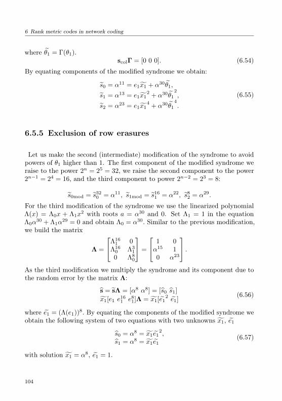
6 Rank metric codes in network coding
where θ1 = Γ(θ1).scolΓ = [0 0 0]. (6.54)
By equating components of the modified syndrome we obtain:
s0 = α11 = e1x1 + α30θ1,
s1 = α13 = e1x12
+ α30θ1
2,
s2 = α23 = e1x14
+ α30θ1
4.
(6.55)
6.5.5 Exclusion of row erasures
Let us make the second (intermediate) modification of the syndrome to avoidpowers of θ1 higher than 1. The first component of the modified syndrome weraise to the power 2n = 25 = 32, we raise the second component to the power2n−1 = 24 = 16, and the third component to power 2n−2 = 23 = 8:
s0mod = s320 = α11, s1mod = s16
1 = α22, s82 = α29.
For the third modification of the syndrome we use the linearized polynomialΛ(x) = Λ0x + Λ1x
2 with roots a = α30 and 0. Set Λ1 = 1 in the equationΛ0α
30 + Λ1α29 = 0 and obtain Λ0 = α30. Similar to the previous modification,
we build the matrix
Λ =
Λ161 0
Λ160 Λ3
1
0 Λ80
=
1 0α15 10 α23
.As the third modification we multiply the syndrome and its component due tothe random error by the matrix Λ:
s = sΛ = [α8 α8] = [s0 s1]
x1[e1 e161 e8
1]Λ = x1[e12 e1]
(6.56)
where e1 = (Λ(e1))8. By equating the components of the modified syndrome weobtain the following system of two equations with two unknowns x1, e1
s0 = α8 = x1e12,
s1 = α8 = x1e1(6.57)
with solution x1 = α8, e1 = 1.
104

6 Rank metric codes in network coding
6.5.6 Correction of random error
Trying all field elements we solve the equation
x1 = α8 = x21 + α5x1.
There are two solutions: x1 = α12 or x1 = α27. Similarly we solve
e1 = 1 = (α30e1 + e21)8.
There are two solutions: e1 = α5 or e1 = α26.Let us use the first solutions: x1 = α12 and e1 = α5. Given x1, let us find
the components of the vector u1 using
x1 = α12 = α2u11 + α29u12 + α5u13 + α14u14 + α9u15 (6.58)
we obtain a solution u1 = [0 1 0 1 1].Write the random error in the vector form: erand = e1u1 = α5[0 1 0 1 1].Transform the random error to the matrix form:
Erand =
10100
[ 0 1 0 1 1]
=
0 1 0 1 10 0 0 0 00 1 0 1 10 0 0 0 00 0 0 0 0
.
6.5.7 Erasure correction
Substitute the known values of s0 = α11, e1 = α5, x1 = α8, a = α30 to thefirst equation of the system (6.55). Solving the equation
α11 = α5α8 + α30θ1.
we obtain θ1 and obtain solutions θ1 = α7 or θ1 = α10.We use (6.48) for θ1 and substitute the solution θ1 = α7. Solve the equation
α7 = α2r11 + α29r12 + α5r13 + α14r14 + α9r15
105

6 Rank metric codes in network coding
and obtain: r1 = [0 1 0 1 0]. The vector of row erasures is erow = α30[0 1 0 1 0],i.e., in matrix form
Erow =
01001
[ 0 1 0 1 0]
=
0 0 0 0 00 1 0 1 00 0 0 0 00 0 0 0 00 1 0 1 0
.To find w1 we substitute to first equation of the main system (6.50):
s0 = e1x1 + α30θ1 + α5w1 = α5,
the known values x1 = α12, e1 = α5, θ1 = α7. We obtain w1 = α8. The columnerasures in vector form are ecol = α8[0 0 1 0 0], and in matrix form
Ecol =
10110
[ 0 0 1 0 0]
=
0 0 1 0 00 0 0 0 00 0 1 0 00 0 1 0 00 0 0 0 0
.The error vector is
e = erand + erow + ecol
= [0 α5 0 α5 α5] + [0 α30 0 α30 0] + [0 0 α8 0 0]
= [0 α26 α8 α26 α5].
(6.59)
Let us check the solution. Subtract from the received vector y (6.43) the errorvector (6.59):
y + e = [α α5 α12 α18 α29] + [0 α26 α8 α26 α5]= [(α+ 0) (α5 + α26) (α12 + α8) (α18 + α26) (α29 + α5)]= [α α30 α18 α7 α20].
(6.60)
Comparing the solution with the transmitted code vector (6.35), we see thatthey coincide.In matrix form the error is
E = Erand + Erow + Ecol =
0 1 1 1 10 1 0 1 00 1 1 1 10 0 1 0 00 1 0 1 0
. (6.61)
106

6 Rank metric codes in network coding
The rank of the error matrix is 4.The difference of the received matrix R and error matrix E (6.61) is
R + E =
0 1 0 1 11 0 1 1 00 1 1 0 00 0 1 0 10 0 0 0 0
+
0 1 1 1 10 1 0 1 00 1 1 1 10 0 1 0 00 1 0 1 0
=
0 0 1 0 01 1 1 0 00 0 0 1 10 0 0 0 10 1 0 1 0
= M.
(6.62)The solution is correct since the code matrix M was transmitted.
6.6 Conclusions
We have considered the principles suggested by Kötter, Kschischang, Silva fordesigning subspace codes based on rank Gabidulin codes. The code matricesconsist of the identity matrix and a matrix of the rank code. This construction iscalled the lifting of rank codes. The network channel forms linear combinationsof rows of a code matrix and adds outer errors. The decoding algorithm consistsof two steps: first obtain the distorted matrix of the rank code using Gaussianelimination and then use a standard algorithm for decoding rank codes.
107


7Multicomponent prefix codes
In this chapter, we introduce a class of codes that is called multicomponent prefixcodes. These codes generalize the codes of Silva-Kötter-Kschischang (SKK). Amulticomponent code is a union of different component codes that are SKKcodes with a fixed code distance, and the minimum subspace distances betweenthe code components are not less than the code distance of the components.
7.1 Gabidulin–Bossert subspace codes
Subspace codes with maximum code distance were proposed by Gabidulin andBossert in [GB08].
Lemma 7.1. Let U and V be subspaces of N-dimensional vector space. Thesubspace distance between them is d(U, V ) = N , if and only if
1. Subspaces U and V intersect trivially, i.e., the intersection is the subspaceof dimension zero.
2. The dimension of the union is dim(U) + dim(V ) = N .
Proof. If both conditions are satisfied then from (6.2) it follows that d(U, V ) =dim(U) + dim(V )− 2 dim(U ∩ V ) = N since dim(U ∩ V ) = 0.
109
7 Multicomponent prefix codes
Assume now that d(U, V ) = N . Denote Z = U ∩ V . We have
d(U, V ) = dim(U) + dim(V )− 2 dim(Z) = N,dim(U ] V ) = dim(U) + dim(V )− dim(Z) ≤ N,dim(Z) ≥ 0.
(7.1)
The system of equations (7.1) has a unique solution dim(Z) = 0. This meansthat the subspaces U and V intersect trivially and dim(U) + dim(V ) = N .
Let C be a code with maximum subspace distance d(C) = N .
Theorem 7.2. If N is odd, then the cardinality of any code C with subspacedistance N is |C| = 2. Such a code consists of two subspaces C = U, V , whereU and V intersect trivially and
dim(U) + dim(V ) = N. (7.2)
Proof. The code C has at most 2 subspaces. Otherwise, at least two subspaceswould have dimensions of the same parity and an even distance d ≤ N betweenthem. The second part of the theorem follows from Lemma 7.1.
The situation changes drastically if N is even, N = 2m.
Lemma 7.3. If the code C with the maximum (even) distance N consists of|C| ≥ 3 subspaces, then the subspaces pairwise intersect trivially and have equaldimension N/2 = m.
Proof. Let a code C consist, for example, of 3 subspaces U1, U2, U3. By Lemma7.1, any pair of subspaces intersect trivially. In addition to this dim(U1) +dim(U2) = 2m, dim(U1) + dim(U3) = 2m, dim(U3) + dim(U2) = 2m. Hence,dim(U1) = dim(U2) = dim(U3) = m.
Lemma 7.4. The cardinality of a code C with maximum even distance N = 2msatisfies the bound
|C| ≤ qm + 1. (7.3)
Proof. Every m-dimensional subspace has qm − 1 nonzero vectors from N -dimensional vector space. The number of nonzero vectors in C equals |C|(qm−1),since the subspaces of the code C intersect trivially. The relation |C|(qm − 1) ≤qN − 1 = q2m − 1 holds, and we have, |C| ≤ qm + 1.
110
7 Multicomponent prefix codes
Theorem 7.5. There exists a code C with maximum even distance N = 2mand with maximum cardinality
|C| = qm + 1. (7.4)
Proof. Represent m-dimensional subspace by m×2m basis matrices of full rank[C D], where C and D are square matrices of order m. Let A be a matrix oforder m that represents the field Fqm (6.9). Define the set of m-dimensionalsubspaces in C by the following basis matrices:
[Im Om], [Im Im], [Im A], · · · , [Im Aqm−2], [Om Im]. (7.5)
The number of matrices in this set is qm + 1. Each matrix has full rank m.Hence, the corresponding subspaces have rank m each. Let us show that thesesubspaces pairwise intersect trivially. Denote by S the subspace generatedby the matrix M(S) = [Im Om], by Vj , j = 0, . . . , qm − 2 denote subspacesgenerated by the matrices M(Vj) = [Im Aj ], and by R the subspace generatedby the matrix M(R) = [Om Im]. Then we have
dim(S ] Vj) = Rk
([Im OmIm Aj
])= 2m ⇒ dim(S ∩ Vj) = 0,
dim(S ]R) = Rk
([Im OmOm Im
])= 2m ⇒ dim(S ∩R) = 0,
dim(Vi ] Vj) = Rk
([Im Ai
Im Aj
])= 2m ⇒ dim(Vi ∩ Vj) = 0,
dim(Vi ]R) = Rk
([Im Ai
Om Im
])= 2m ⇒ dim(Vi ∩R) = 0.
Hence, the code defined by (7.5) is an optimal code with distance N = 2m.
7.2 Multicomponent Gabidulin-Bossert subspacecodes
New subspace codes based on rank codes were proposed by Gabidulin andBossert [GB09] and were called multicomponent prefix codes. Let us considerconstructions of these codes.
111

7 Multicomponent prefix codes
Write N = m1 + m2 + · · · + mk, where m1 ≥ m2 ≥ · · · ≥ mk. We willdesign a code X as the union of component codes X = X1 ∪ X2 ∪ · · · ∪ Xk.Pairwise intersection of the component codes should be empty. Let us definethe component codes as follows:
X1 =X : X =
[Im1 x1
]| x1 ∈M1
X2 =
X : X =
[Om1m2
Im2 x2
]| x2 ∈M2
...Xk−1 =
X : X =
[Om1+···+mk−2mk−1 Imk−1
xk−1
]| xk−1 ∈Mk−1
Xk =
X : X =
[ON−mkmk
Imk].
(7.6)
Here
• M1 is a rank code consisting of m1 × (N −m1) matrices over Fq withrank code distance dr1 ≤ minm1, N −m1;
• M2 is a rank code consisting of m2 × (N −m1 −m2) matrices over Fqwith rank code distance dr2 ≤ minm2, N −m1 −m2;
•...
• Mk−1 is a rank code consisting of mk−1× (N−m1−· · ·−mk−1) matricesover Fq with rank code distance dr (k−1) ≤ minmk−1, N −m1 − · · · −mk−1.
Obviously, Xi ∩ Xj = ∅, i 6= j.The code has the following characteristics:
• cardinality
X = |C| =k∑i=1
|Ci| ,
• subspace distance
d(X ) = minmini6=j
(mi +mj), min1≤i≤k−1
2dri.
112

7 Multicomponent prefix codes
7.3 Decoding codes with maximum distance
First consider the subspace code of length N consisting of two subspaces: thefirst is generated by rows of the identity matrix X1 = IN , the second by rowsof all zero matrix X2 = ON .If the matrix X1 has been transmitted, then the received matrix is
Y = AX1 +BZ = A+BZ,
if X2 was transmitted, then the received matrix is
Y = AX2 +BZ = BZ.
The decoder computes rank Rk(Y ) of the received matrix Y and the distancebetween the subspace 〈Y 〉 and 〈X1〉 and 〈X2〉 respectively:
d1 = d(〈Y 〉, 〈X1〉) = 2Rk
([YIN
])− Rk(Y )− Rk(IN ) = N − Rk(Y )
and
d2 = d(〈Y 〉, 〈X2〉) = 2Rk
([YON
])− Rk(Y )− Rk(ON )
= 2Rk(Y )− Rk(Y ) = Rk(Y ).
If d1 < d2, i.e., Rk(Y ) > N/2, then the decoder makes a decision X1 = IN ,otherwise the decision is X2 = ON .
For N = 2m, the code X with maximum subspace distance 2m can be seenas the union of two subcodes X = X1 ∪ X2, where
X1 =X : X =
[Im x
], x ∈ C
is the code of cardinality qm having a single m×m code matrix x of the rankcode, and
X2 =X : X =
[Om Im
]is the code of cardinality 1.Let the received matrix be
Y = AX +BZ =[A y
].
113

7 Multicomponent prefix codes
Decoding consists of two steps. In the first step, the decoder tries to determinewhether the received subspace 〈Y 〉 corresponds to the transmitted matrix X1
or X2. This is equivalent to finding whether the subspace 〈A〉 originates from〈Im〉 or from 〈Om〉. It was shown above that the solution is based on the rankof the matrix Rk(A):
• If Rk(A) < m/2, then the subspace 〈Y 〉 originates from X2. Then we goto the second step: consider the matrix
[Om Im
]as the decoding result.
• If Rk(A) ≥ m/2, then the subspace 〈Y 〉 originates from X1. Go tothe second step: run SKK decoder, extract the matrix x ∈ C and getX =
[Im x
]as the decoding result.
7.4 Decoding multicomponent prefix codes
Let us generalize the approach we considered for decoding multicomponentcodes. Let Y be a received matrix
Y = AX +BZ
and X belongs to one of the component codes (7.6). Write Y as
Y =[A1 A2 . . . Ak−1 y
],
where A1 is an nr × m1 matrix, A2 is an nr × m2 matrix, . . . , Ak−1 is annr ×mk−1 matrix.
• The decoder should solve the following problem: does the received subspace〈Y 〉 originate from the subcode X1or from X2 ∪ · · · ∪ Xk? Instead, thedecoder solves an equivalent problem: does the subspace 〈A1〉 originatefrom the subspace 〈Im1
〉 or from 〈Om1〉? To find the solution, the decoder
computes the rank of A1: r1 = Rk(A1).
1. If r1 ≥ m1/2, then the decision is: 〈Y 〉 originates from X1. Usingthe SKK decoder, find x1 ∈ M1. The decoder outputs the matrixX =
[Im1
x1
]as the decoding result.
114
7 Multicomponent prefix codes
2. If r1 < m1/2, then the decision is: 〈Y 〉 originates from the subcodeX2 ∪ · · · ∪ Xk. The decoder goes to the next step.
• The decoder should solve the following problem: does the received subspace〈Y 〉 X2 or from the subcode X3 ∪ · · · ∪ Xk? Instead, the decoder solves anequivalent problem: does the subspace
⟨[A1 A2
]⟩originate from the
subspace⟨[Om1m2
Im2
]⟩or from
⟨[Om1m2
Om2
]⟩? To find the solution,
the decoder computes the rank r2 = Rk([A1 A2
]).
1. If r2 ≥ m2/2, then the desicion is: 〈Y 〉 originates from the subcodeX2. Using the SKK decoder to find x2 ∈ M2. The matrix X =[Om1m2
Im2 x2
]is the decoding result.
2. If r2 < m2/2, then the decision is: 〈Y 〉 originates from the subcodeX3 ∪ · · · ∪ Xk. The decoder goes to the next step.
• The algorithm is running until the final decision is found. The number ofrequired steps is k at most.
7.5 Cardinality of MZP codes
The multicomponent codes with zero prefix (MZP) were presented in 2008 byGabidulin and Bossert [GB08]. They were based on the lifted rank codes byKötter, Kschischang, Silva [KK08], [SKK08]. Let n = m+rδ+s be code length,where m is the dimension, r is an integer, r ≥ 1, 0 ≤ s ≤ δ − 1.
The first component is the SKK-code. It consists of a set of matrices
Cskk =(
Im M1
)|M1 ∈M1
, (7.7)
where Im is the identity matrix of order m, while M1 is a code matrix of sizem× (n−m) of the rank matrix codeM1 with rank distance drank = δ [Gab85].The subspace distance of the code Cskk is more than twice the rank distance ofthe matrix codeM1: dsub(Cskk) = 2drank(M1) = 2δ.
The cardinality of a subspace code is a very important characteristic. Thereare many works which estimate this characteristic and compare it with upperbounds (see, for example, [GP17b], [GP17a]) .
115
7 Multicomponent prefix codes
The cardinality |Cskk| of SKK-code is equal to the size of the rank code withrank distance drank = δ and code length (n−m) :
|Cskk| = q(n−m)(m−δ+1), (7.8)
where δ ≤ m,n ≥ 2m.For i = 2, . . . , r, the (i)-th component consists of matrices of the form
Cmzp i =(
0δm . . . 0δm Im Mi
)|Mi ∈Mi
,
where the first i− 1 block matrices are the all-zero matrices 0δm of size m× δ.Im is the identity matrix, Mi is a code matrix of size m× (n−m− (i− 1)δ)of the rank matrix codeMi with rank distance δ. The cardinality of the ithcomponent is as follows:
|Cmzp i| = q(n−m−(i−1)δ)(m−δ+1) = qni(m−δ+1), (7.9)
where ni = n − m − (i − 1)δ is the code length of the rank code. The lastcomponent is the concatenation of all-zero matrix of size m × (n − m), theidentity matrix IM , and a matrix Asm of size m× s which may have a rank lessthan or equal to s ≤ δ − 1. Hence the last component delivers only one codematrix. The total number of components is equal to l + 1. The cardinality ofthe MZP code is the sum of the cardinalities of all components because thecomponents do not intersect:
Mmzp = |Cmzp| =l∑i=1
q((n−m)−(i−1)δ)(m−δ+1) + 1. (7.10)
7.6 Additional cardinality
In many articles the most attention is given to SSK codes as subspace codesobtained by lifting of rank codes. The cardinality of the lifting codes obtainedcan differ just by one code word, but this code word is not known. This casecorresponds to our two components code and we use the last word. In matrixpresentation it is the concatenation of zero matrix and the identity matrix.
Here, we show that multicomponent code can increase cardinality by consid-erably more than one code word. Let us construct the multicomponent code,
116

7 Multicomponent prefix codes
where n is code length, m is dimension, d = 2δ is code distance. The cardinalityof each component is the following:
Mskk = M1 = q(m−δ+1)(n−m);
M2 = q(m−δ+1)(n−m−δ);
Mi = q(m−δ+1)(n−m−(i−1)δ).
Let the total number of components be (i+1), where n−m− (i− 1)δ = m, thatis i = 1 + n−2m
δ . The last component is a concatenation of the all-zero matrixof size m× (n−m), the identity matrix Im, and a matrix Asm.The total cardinality is
Mmzp = qk(n−m) +qk(n−m−δ)qkδ − qkm
qkδ − 1+ 1 = Mskk + ∆,
where k = m− δ + 1 and
∆ =qk(n−m−δ)qkδ − qkm
qkδ − 1+ 1.
∆ is the number of additional words except words of the first component.Now, let us estimate the ratio that is the additional cardinality to the first
component cardinality ν = ∆Mskk
.
ν =1
qkδ − 1− qkm − qkδ + 1
(qkδ − 1)qk(n−m).
ν ' 1
qkδ − 1
under the condition
qk(n−m)(qkm−qkδ+1qkm−qkδ+1).
If m = δ, k = 1, then this condition is the following
qk(n−m) 1,
and it is evident that Mskk = qk(n−m). Let us give numerical examples. Theyare shown in Table 7.1.
117
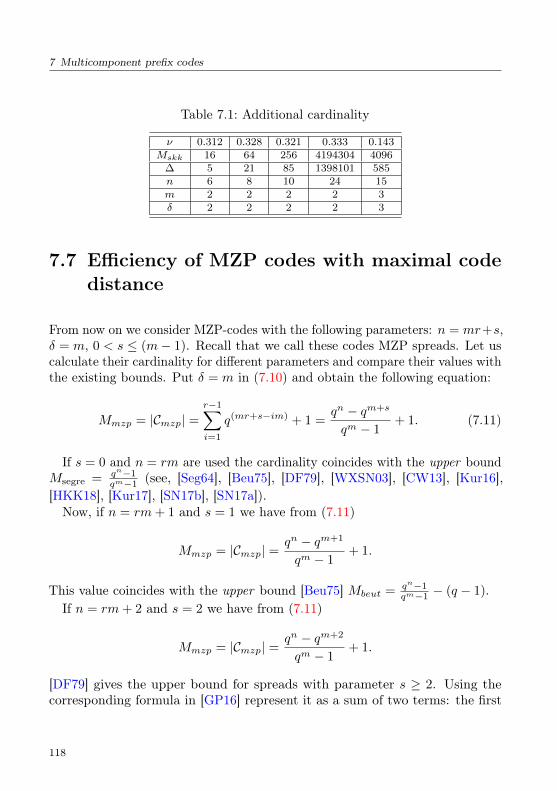
7 Multicomponent prefix codes
Table 7.1: Additional cardinality
ν 0.312 0.328 0.321 0.333 0.143Mskk 16 64 256 4194304 4096
∆ 5 21 85 1398101 585n 6 8 10 24 15m 2 2 2 2 3δ 2 2 2 2 3
7.7 Efficiency of MZP codes with maximal codedistance
From now on we consider MZP-codes with the following parameters: n = mr+s,δ = m, 0 < s ≤ (m− 1). Recall that we call these codes MZP spreads. Let uscalculate their cardinality for different parameters and compare their values withthe existing bounds. Put δ = m in (7.10) and obtain the following equation:
Mmzp = |Cmzp| =r−1∑i=1
q(mr+s−im) + 1 =qn − qm+s
qm − 1+ 1. (7.11)
If s = 0 and n = rm are used the cardinality coincides with the upper boundMsegre = qn−1
qm−1 (see, [Seg64], [Beu75], [DF79], [WXSN03], [CW13], [Kur16],[HKK18], [Kur17], [SN17b], [SN17a]).Now, if n = rm+ 1 and s = 1 we have from (7.11)
Mmzp = |Cmzp| =qn − qm+1
qm − 1+ 1.
This value coincides with the upper bound [Beu75] Mbeut = qn−1qm−1 − (q − 1).
If n = rm+ 2 and s = 2 we have from (7.11)
Mmzp = |Cmzp| =qn − qm+2
qm − 1+ 1.
[DF79] gives the upper bound for spreads with parameter s ≥ 2. Using thecorresponding formula in [GP16] represent it as a sum of two terms: the first
118

7 Multicomponent prefix codes
term is the cardinality of the MZP spread and the second is γ1, where γ1 issome quantity.
Mdr−fr ≤qn − qm+s
qm − 1+ 1 + γ1, (7.12)
where γ1 = (qs − bθc) − 2, parameter θ depends on m and s in the followingway:
bθc =
qs−1 − 1, if 2s < m+ 2;qs−1 − 2, if 2s = m+ 2;qs−1 − 22s−m−3 − 1, if 2s > m+ 2.
Let q = 2, m = 3 and s = 2. Then γ1 = 1. In this case the cardinality of thisMZP spread does not coincide with the upper bound with difference 1. Toincrease cardinality up to the upper bound in the paper [GP16] a subspace codefrom the paper [EZJS+10] was used. It was obtained there for parameters r = 2,m = 3, s = 2, n = 8 by exhaustive search. We used it as the last componentMZP code for n = mr + 8, where m = 3.Here, for q = 2, r ≥ 2, m = 4 and s = 2 we use the upper bound from the
paper [Kur16]:
MKurz =24r+2 − 49
15. (7.13)
Applying our formula for cardinality to the MZP spread (7.11) with the sameparameters, one can see that the cardinality of the MZP spread coincides withthis upper bound.Now we will use the upper bounds from [HKK18]. In this paper there are
two important theorems. Let us give our interpretation and our designationsfor these theorems.
Theorem 7.6. If 0 < s < m and m > qs, then the maximal cardinality ofsubspace code is the following: MHKK1 = qmr+s−qm+s+qm−1
qm−1 .
Let us compare MHKK1 (7.6) and Mmzp (7.11). One can see that bothformulas for cardinality coincide. That means that the cardinality of the MZPspread achieves the upper bound if the conditions indicated in the theorem aresatisfied: 0 < s < m and m > qs.If the conditions are not satisfied there is another theorem in the paper
[HKK18].
119

7 Multicomponent prefix codes
Theorem 7.7. If 0 < s ≤ (m− 1) and m < qs, then the maximal cardinalityof subspace code is the following: MHKK2 = qn−qm+s+qm−1
qm−1 + γ2, where γ2 > 1,it is calculated by means of auxiliary parameters.
We see that the MZP spread does not coincide with the upper bound at theseconditions.There are two values γ2: γ21 > 1 and γ22 > 1. We have
γ21 = d2m − 1
2(1 + 2m+2(2m − 2s))
12 e − 1
and
γ22 = d2s − 1
2(1 + 2s+2(m− s)) 1
2 e − 1.
For γ2 one should select the minimum between γ21 and γ22.We would also like to estimate by Drake–Freeman [DF79]. For this purpose
we will use the parameter γ1 = (qs − bθc) − 2. At the chosen parameters wecalculate three values γ1, γ21 and γ22, take the smallest value and add to thecardinality value of the MZP spread. We consider the value obtained as anestimation Mup of the upper bound at these conditions. The efficiency of theMZP spread is denoted η =
Mmzp
Mup.
Table 7.2: Efficiency of MZP spread
η 0.971 0.970 0.985 0.996 0.992 0.997 0.996Mmzp 33 129 513 513 2049 2049 4097Mup 34 133 521 515 2066 2055 4112n 8 11 14 15 17 18 19m 3 4 5 6 6 7 7s 2 3 4 3 5 4 5γ21 1 4 8 2 18 6 15γ22 1 5 11 3 25 7 22γ1 1 4 10 3 17 7 19
One can see from Table 7.2 that the efficiency η =Mmzp
Mupis about η = 0.99
for all the cases where m < 2s.
120

7 Multicomponent prefix codes
7.8 Dual multicomponent codes
Let a subspace X of dimension m be given by a matrix L of size m× n withrank m. The orthogonal subspace X⊥ of dimension n−m will be given by thematrix L⊥ of size (n−m)× n such that
(L⊥)(L>) = 0,
where L> means the transposed matrix L.Let us construct the dual multicomponent code (DMC). For j = 1, . . . r, the
components of the MZP codes with dimension m and length n = rm+ s aregiven by matrices of rank m with the following form:
Lj =[0m . . . 0m Im Mj
].
The matrices consist of the zero matrix prefix of size m× (j − 1)m, the unitysubmatrix Im of order m and the submatrix Mj of size m× n− jm.The orthogonal matrixL⊥j with rank n−m is the following
L⊥j =
[I(j−1)m 0m(j−1)m 0n−jm(j−1)m
0(j−1)mn−jm −M> In−jm
],
where 0vl is the zero matrix of size l × v.DMC code L⊥j has dimension n−m and subspace code distance dsub = 2m.
For the parameters n = mr + s,m = 2, 3, s = 0, 1 these codes have maximalcardinality.
7.9 Maximal cardinality MZP and DMC codes
First we consider MZP code. Let the parameters be δ = m and n = (r + 1)m+s, s = 0. Then
Mmzp =
r−1∑i=1
q(r−i+1)m(m−m+1) + 1 =qn − 1
qm − 1.
This formula coincides with the upper bound Mmax(0) [WXSN03].
121

7 Multicomponent prefix codes
Now n = (r + 1)m+ 1, s = 1, then
Mmzp = qq(r+1)m − 1
qm − 1− (q − 1).
This formula coincides with the more precise upper bound
Mmax(1) = qq(r+1)m − 1
qm − 1− (q − 1).
It means that for m = 2 the MZP codes have the maximal cardinality for anyvalue of the parameters n, d. If m = 3 the MZP codes have maximal cardinalityat δ = 3 and n = (r+ 1)m+ s, s = 0, 1. The corresponding dual codes have thesame cardinality at the same parameters except dimension, which is m′ = n−m.
Example 8. Let us construct MZP codes with parameters n = (2× 3) + 1 =7, d = 6 and the corresponding dual code with dimension n− 3 = 4. In this casethe MZP code consists of two components.
The first component is concatenation of two matrices I3 of order 3 andthe matrix M of size 3 × 4 of the rank code. The second component is alsoconcatenation of two matrices. The first matrix is zero matrix 04
3 of size 3× 4,the second matrix is the identity matrix I3 of order 3. The cardinality of thefirst component is M1 = 24, the cardinality of the second component is M2 = 1.The total cardinality is Mmax = 17. This value coincides with the upper bound.
The corresponding dual code also consists of two components. The firstcomponent is concatenation of two matrices, where the first matrix is thetransposed 4× 3 matrix −MT of the rank code and the initial MZP code hasdimension 3. In this case the code word length is not equal to the doubledimension (2×m′ = 8). Nevertheless, this dual code has maximal cardinality.This small example shows that construction of dual codes increases the generalnumber of codes with maximum cardinality.
7.10 ZJSSS codes with maximal cardinality
Now let us use the following parameters: (n = rm + 2) = 8, m = 3. In thiscase our MZP code has cardinality M = 33, but the upper bound is one wordgreater, that is Mmax = 34.
122
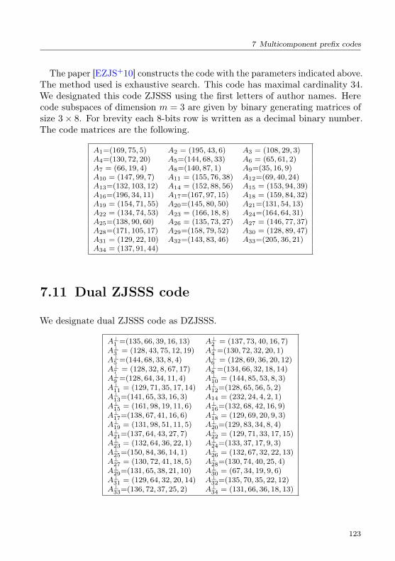
7 Multicomponent prefix codes
The paper [EZJS+10] constructs the code with the parameters indicated above.The method used is exhaustive search. This code has maximal cardinality 34.We designated this code ZJSSS using the first letters of author names. Herecode subspaces of dimension m = 3 are given by binary generating matrices ofsize 3× 8. For brevity each 8-bits row is written as a decimal binary number.The code matrices are the following.
A1=(169, 75, 5) A2 = (195, 43, 6) A3 = (108, 29, 3)A4=(130, 72, 20) A5=(144, 68, 33) A6 = (65, 61, 2)A7 = (66, 19, 4) A8=(140, 87, 1) A9=(35, 16, 9)A10 = (147, 99, 7) A11 = (155, 76, 38) A12=(69, 40, 24)A13=(132, 103, 12) A14 = (152, 88, 56) A15 = (153, 94, 39)A16=(196, 34, 11) A17=(167, 97, 15) A18 = (159, 84, 32)A19 = (154, 71, 55) A20=(145, 80, 50) A21=(131, 54, 13)A22 = (134, 74, 53) A23 = (166, 18, 8) A24=(164, 64, 31)A25=(138, 90, 60) A26 = (135, 73, 27) A27 = (146, 77, 37)A28=(171, 105, 17) A29=(158, 79, 52) A30 = (128, 89, 47)A31 = (129, 22, 10) A32=(143, 83, 46) A33=(205, 36, 21)A34 = (137, 91, 44)
7.11 Dual ZJSSS code
We designate dual ZJSSS code as DZJSSS.
A⊥1 =(135, 66, 39, 16, 13) A⊥2 = (137, 73, 40, 16, 7)A⊥3 = (128, 43, 75, 12, 19) A⊥4 =(130, 72, 32, 20, 1)A⊥5 =(144, 68, 33, 8, 4) A⊥6 = (128, 69, 36, 20, 12)A⊥7 = (128, 32, 8, 67, 17) A⊥8 =(134, 66, 32, 18, 14)A⊥9 =(128, 64, 34, 11, 4) A⊥10 = (144, 85, 53, 8, 3)A⊥11 = (129, 71, 35, 17, 14) A⊥12=(128, 65, 56, 5, 2)A⊥13=(141, 65, 33, 16, 3) A14 = (232, 24, 4, 2, 1)A⊥15 = (161, 98, 19, 11, 6) A⊥16=(132, 68, 42, 16, 9)A⊥17=(138, 67, 41, 16, 6) A⊥18 = (129, 69, 20, 9, 3)A⊥19 = (131, 98, 51, 11, 5) A⊥20=(129, 83, 34, 8, 4)A⊥21=(137, 64, 43, 27, 7) A⊥22 = (129, 71, 33, 17, 15)A⊥23 = (132, 64, 36, 22, 1) A⊥24=(133, 37, 17, 9, 3)A⊥25=(150, 84, 36, 14, 1) A⊥26 = (132, 67, 32, 22, 13)A⊥27 = (130, 72, 41, 18, 5) A⊥28=(130, 74, 40, 25, 4)A⊥29=(131, 65, 38, 21, 10) A⊥30 = (67, 34, 19, 9, 6)A⊥31 = (129, 64, 32, 20, 14) A⊥32=(135, 70, 35, 22, 12)A⊥33=(136, 72, 37, 25, 2) A⊥34 = (131, 66, 36, 18, 13)
123

7 Multicomponent prefix codes
7.12 The family of MZP and combined codes
The algorithm of MZP code construction makes it possible to input ZJSSS codeas two last components in order to increase cardinality of the MZP code.
Example 9. Let n = 11. The MZP code consists of 3 components.
The first component is SKK . Let us substitute the last two components ofMZP code for the code ZJSSS, where we add zero prefix matrix 03 of order 3.The cardinality of this ZJSSS code is 34 which is maximal for chosen parametersn = 8 and d = 2m = 6. We have obtained a two component combined [11, 6, 3]MZP-ZJSSS code with maximal cardinality 290.
Table 7.3: Cardinality of MZP and MZP-ZJSSS codes
r n Mmax Mmzp Mmax −Mmzp
2 8 34 33 13 11 290 289 14 14 2338 2337 15 17 18722 18721 1
Use the same method and set parameters n = 3(r−1)+8 = 3(r+1)+2, m = 3,d = 6. We will obtain a family of subspace codes with maximal cardinality. Firstof all, we construct an MZP-ZJSSS code with code word length n = 3× r + 2,where r is an integer. For example r = 2, 3, 4, 5, n = 8, 11, 14, 17. Let uscalculate the cardinality of MZP and MZP-ZJSSS codes. We put this data inthe Table 7.3.
Example 10. Two component combined MZP-ZJSSS code). Using combinedMZP-ZJSSS code with parameters n = 11, m = 3, d = 6, we construct acombined dual two component code and designate it by CD2C.
The first component is given by the matrix:[MT I8
].
The second component is given by the matrix:[I3 08
3
035 Z⊥
],
124

7 Multicomponent prefix codes
where Z⊥ is a DZJSSS code matrix with size 5 × 8. The matrix with size8× 11 is a concatenation of two submatrices, where the first submatrix MT isa transposed rank code matrix of size 3× 8, and the second submatrix is theidentity matrix I8 of order 8. The second component is the dual ZJSSS code inthe form of the general matrix of size 8× 11. The general matrix consists offour submatrices: the identity matrix I3 of order 3 is located in the left uppercorner, the zero matrix 08
3 with size 3× 8 is located in the right upper corner,the zero matrix 03
5 of size 5× 3 is located in the left down corner, the matrix ofsize 5× 8 is located in the right down corner. This matrix is orthogonal to theZJSSS code matrix of size 3× 8.
Example 11. Three component combined MZP-ZJSSS code.
We construct a three component combined MZP-ZJSSS code with maximalcardinality with the following parameters: code word length n = 14, dimensionm′ = n − m = 14 − 3 = 11. The matrix of the first component is in theform [I3 M11 M12 M13 M14] , where the rank code matrix M1 is written as theconcatenation of four matrices M1 = [M11M12M13M14], where the size of eachof the first three matrices is 3× 3, the size of the fourth matrix is 3× 2. Thecorresponding first component of the dual code is in the form:
MT11 I3 03 03 02
MT12 03 I3 03 02
MT13 03 03 I3 02
MT14 03 03 03 I2
.The second component of the MZP code is the following
[03
3 I3 M21 M22 M23
],
where the rank code matrix M2 is in the form of concatenation of three matricesM2 = [M21 M22 M23]. The size of each of the first three matrices is 3× 3, thesize of the fourth matrix is 3× 2. The corresponding second component of thedual code is
I3 03 03 03 02
03 MT21 I3 03 02
03 MT22 03 I3 02
03 MT23 03 03 I2
.The third component of the combined three component code is presented asthe concatenation of two zero matrices with size 3× 3 and the matrix of theZJSSS code with size 3× 8: [
033 03
3 Z],
125

7 Multicomponent prefix codes
where Z is a matrix of the ZJSSS code. The corresponding third component ofthe dual code is the following: I3 03
3 083
033 I3 08
3
035 03
5 ZT
,where ZT is a transposed matrix with size 5× 8 of the ZJSSS code.
7.13 MZP codes with dimension m ≥ 4 and dualcodes
In [Kur17] it is shown that the upper bound is equal to Mmax = 2m+2 + 1 if theparameters are the following n = 2m+ 2, m ≥ 4, d = 2m. Our two componentMZP code has this cardinality.
Let m = 4, n = 10, d = 8. The first component is SKK code with the matrix[I4 M11 M12] and the cardinality M1 = 2m+2 = 64, the second component isthe identity matrix with zero prefix which is a zero matrix with size 4× 6. Thecardinality of the second component is one code word.The corresponding dual code also consists of two components. The first
component is [MT
11 I4 024
MT12 04
2 I2
].
The second component is [I4 04
4 024
042 04
2 I2
].
The new dimension is m′ = n −m = 10 − 4 = 6. As one can see the doublevalue of dimension 2m′ = 12 does not coincide with the code distance d = 8.Let n = 3m+ 2 = 14, m = 4, d = 8. The initial three component code isI4 M11 M12 M13
044 I4 M21 M22
044 04
4 024 I4
,where each matrix row is the corresponding component, each of the matricesM11, M12, M21 has size 4× 4, the size of each matrices M13 and M2 is 4× 2
126

7 Multicomponent prefix codes
The first component of the dual code is in the formMT11 I4 04
4 024
MT12 04
4 I4 024
MT13 04
2 042 I2
,The second component of the dual code is in the formI4 04
4 044 02
4
044 MT
21 I4 024
042 MT
22 042 I2
.The third component of the dual code is in the formI4 04
4 044 02
4
044 I4 04
4 024
042 04
2 042 I2
.
7.14 Conclusions
This chapter is devoted to multicomponent subspace codes. We have shownthe place of these codes in random network coding. We have described theconstructions and have estimated the cardinality of the codes. The efficiencyof the MZP codes is defined as ratio of its cardinality to the upper bound atthe same parameters. At maximum code distance, the efficiency is maximum,i.e., it is equal to 1 or near 1. It depends on the dimension. We have alsodemonstrated the iterative decoding algorithm.
127


8Multicomponent codes based oncombinatorial block designs
8.1 Introduction
A code cardinality, i.e., the number of codewords, is an important code pa-rameter. Therefore, researches try to design multicomponent codes with largecardinality and distance d as a union of several codes having the same distanced. The cardinality of a multicomponent code is usually equal to the sum ofthe cardinalities of its components. Etzion and Silbershtein [ES09] show thatprojective spaces can be used to design multicomponent codes.
In this chapter, we will show multicomponent subspace codes, based onrank metric codes and combinatorial block designs [Hal67]. Examples of somemulticomponent subspace codes will be given. Special rank metric codes withrestrictions for these constructions will be considered. We also will pay attentionto the decoding of multicomponent subspace codes in networks.
129
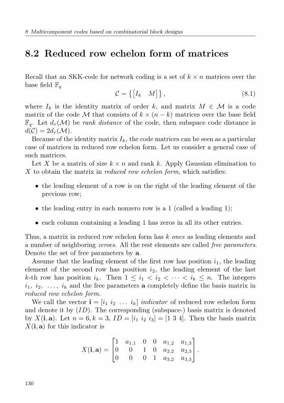
8 Multicomponent codes based on combinatorial block designs
8.2 Reduced row echelon form of matrices
Recall that an SKK-code for network coding is a set of k × n matrices over thebase field Fq
C =[Ik M
], (8.1)
where Ik is the identity matrix of order k, and matrix M ∈ M is a codematrix of the codeM that consists of k × (n− k) matrices over the base fieldFq. Let dr(M) be rank distance of the code, then subspace code distance isd(C) = 2dr(M).
Because of the identity matrix Ik, the code matrices can be seen as a particularcase of matrices in reduced row echelon form. Let us consider a general case ofsuch matrices.Let X be a matrix of size k × n and rank k. Apply Gaussian elimination to
X to obtain the matrix in reduced row echelon form, which satisfies:
• the leading element of a row is on the right of the leading element of theprevious row;
• the leading entry in each nonzero row is a 1 (called a leading 1);
• each column containing a leading 1 has zeros in all its other entries.
Thus, a matrix in reduced row echelon form has k ones as leading elements anda number of neighboring zeroes. All the rest elements are called free parameters.Denote the set of free parameters by a.
Assume that the leading element of the first row has position i1, the leadingelement of the second row has position i2, the leading element of the lastk-th row has position ik. Then 1 ≤ i1 < i2 < · · · < ik ≤ n. The integersi1, i2, . . . , ik and the free parameters a completely define the basis matrix inreduced row echelon form.
We call the vector i = [i1 i2 . . . ik] indicator of reduced row echelon formand denote it by (ID). The corresponding (subspace-) basis matrix is denotedby X(i,a). Let n = 6, k = 3, ID = [i1 i2 i3] = [1 3 4]. Then the basis matrixX(i,a) for this indicator is
X(i,a) =
1 a1,1 0 0 a1,2 a1,3
0 0 1 0 a2,2 a2,3
0 0 0 1 a3,2 a3,3
.
130

8 Multicomponent codes based on combinatorial block designs
This matrix has 7 free parameters ai,j , which can be selected arbitrarily fromthe field Fq. Hence, there are q7 different 3-dimensional subspaces for thisindicator.In general case, the first row has n − k + 1 − i1 free parameters, the j-th
row has n− k + j − ij free parameters, j = 1, . . . , k. The total number of freeparameters is
f =
k∑i=1
fi = nk − (k − 1)k
2− i1 − i2 − · · · − ik. (8.2)
From this example one can see that a code matrix of SKK code is a particularcase of a matrix in reduced row echelon form with the identity matrix on theleft part and a rank code matrix on the right. In other cases, columns of theidentity matrix can occupy other positions, and the remaining positions canbe occupied by columns of a rank code. Keep in mind that some elements ofthese remaining positions must be zero, the other elements, denoted by a in theexample, are free.
8.3 Rank codes with restrictions
Consider a vector MRD [n, k, d]-code with generator matrix G. Let the infor-mation vector be u = (u1, . . . , uk), then the code vector is g(u) = uG,and gives code matrix
M(uG) =
a11 a12 . . . a1n
a21 a22 . . . a2n
......
......
aN1 aN2 . . . aNn
.A code matrix is called a matrix with restrictions if aij = 0 for fixed positions.Rank code with such matrices is called rank code with restrictions.Problem: Given a rank distance, design the rank code with restrictions.Let us solve the problem as follows: find the restrictions on the information
vectors u, design a vector code with these restrictions and transform it to thematrix form.
131

8 Multicomponent codes based on combinatorial block designs
8.4 Singleton bound
First we give the Singleton bound for standard rank codes, then we derive abound for the rank metric codes with restrictions.
Let a rank metric code in matrix form consist of |M | matrices of size N × n,n ≤ N , with rank distance d.Let us obtain an upper bound for |M |. Every code matrix we write as [Ai,
Bi], i = 1, |M |, where matrices Ai have size N × (d − 1), and matrices Bihave size N × (n − d + 1)). All matrices Bi are different, otherwise, if sayB1=B2 then the code matrix [A1 −A2, 0] has rank at most d− 1. For the codewithout restrictions, every matrix Bi has N × (n − d + 1) elements. Hence,the number of code words is upper bounded by qN×(n−d+1), the number ofdifferent matrices Bi. Thus, the Singleton upper bound for a rank metric codeis logq |M | ≤ N × (n− d+ 1). The rank codes we considered before reach thisbound.Let us obtain an upper bound for the cardinality of a rank metric code
with distance d and with restrictions, i.e., there are fixed positions in the codematrices that are always zero. Let us select d − 1 columns with maximumnumber of free elements, move these columns to the left part of the matrixand call the submatrix A. The remaining columns we order in a way that thenumber of free elements decreases from left to right and denote this submatrixby B.Denote the number of free elements in columns of A by N1, N2, . . . , Nd−1,
and for the matrix B by Nd, Nd+1, . . . , Nn. We will use the same derivationas in the case without restrictions. The number of different matrices B isqNd+Nd+1+...+Nn . Hence, the Singleton type bound for a code with restrictionsdepends on the restrictions and has the form |M | ≤ qNd+Nd+1+...+Nn .
Let us show by an example how to compute the bound and design a codethat reaches this bound. Code parameters: q = 2, n = 3, k = 2, d = 2. Theprimitive polynomial to generate the field is α3 + α2 + 1 = 0. The generatormatrix of the rank [3,2,2] code is
G =
[1 α α2
1 α2 α4
]. (8.3)
132

8 Multicomponent codes based on combinatorial block designs
A code matrix with restrictions is
Mrestrict(uG) =
a11 a12 a13
0 a22 a23
0 a32 a33
. (8.4)
To obtain the bound we transpose the matrix. The matrix A has the firstcolumn (of the transposed matrix) that has N1 = 3 free elements. The matrixB has other two columns with Nd + Nn = 2 + 2 = 4 free elements. Hence,|M | ≤ 24 = 16.
Let us show that the [3,2,2] code with restricted information symbols reachesthe Singleton bound. We take 1, α, α2 as the basis of the field F23 . Transform acode matrix into the vector form b = (b1, b2, b3),
b = ((a11 ·1+a21 ·α+a31 ·α2), (a12 ·1+a22 ·α+a32 ·α2), (a13 ·1+a23 ·α+a33 ·α2)).
Here a21 = a31 = 0, hence, b1 = a11.For the information vector (u1, u2) we get the code vector (b1, b2, b3)
(u1, u2)
[1 α α2
1 α2 α4
]= ((u1 + u2), (u1α+ u2α
2), (u1α2 + u2α
4)),
where b1 = a11 = (u1 + u2) , u2 = u1 + a11. Let the information symbol u1 beequal to one of 23 = 8 field elements of F23 . Since a11 can be 0 or 1 only, theinformation symbol u2 = u1 + a11 takes only 2 values for fixed u1. Thus withthe restrictions on information symbols we have 2× 23 = 16 codewords, andthe restricted code reaches the Singleton type bound.Now consider the case d = 3. We will use [3,1,3] rank code with generator
matrixG =
[1 α α2
]. (8.5)
The matrix A has d− 1 = 2 columns, where all elements are free. The matrixB has one column, which contains one free element a11 and two zero elements,and we obtain the bound |M | ≤ 21 = 2.
The information vector of length 1 is (u1). The corresponding code vector isb = (u1)G = (u1, u1α, u1α
2) = (b1, b2, b3). From the restriction (8.4) we haverestriction for the information symbol u1 = a11 ∈ F2. Hence, there are two codewords in the restricted code, and the Singleton type bound is reached.
133

8 Multicomponent codes based on combinatorial block designs
8.5 Combinatorial block designs
To construct multicomponent subspace codes we will use basis matrices of thesubspaces in reduced row echelon form and rank metric codes with restrictions.The multicomponent code is a union of subcodes that are called components ofthe code. To guarantee a fixed subspace distance between code components, wewill use combinatorial block designs [Hal67].
In combinatorial analysis, one of the problems is: place in a special way someelements in given sets. The i-th element should appear ri times in the setssuch that the j-th set contains kj elements, and also pairs, triples and othercombinations of elements should appear a fixed number of times. Such placementis called an incidence structure or tactical configuration. A particular type ofsuch placements is balanced incomplete block designs. By definition, balancedincomplete block design is a placement of v different elements in b blocks, suchthat every block contains exactly K different elements, every element appears inr different blocks, and every pair of different elements ai, aj appears in exactlyλ blocks. In combinatorics, balanced incomplete block designs can be calledsimply block designs or designs. We will mostly use the name combinatorialblock designs.
Given the finite set N = 1, 2, . . . , n and integers K, r, λ ≥ 1, we will builda design, called 2 B-block, as a set of subsets consisting of K elements fromN . The following conditions should be satisfied: the number r of blocks thatcontain i ∈ N does not depend on i, and the number λ of blocks that containdifferent pairs i, j ∈ N also does not depend on i, j. Here:
1. n is the number of elements in N ;
2. b is the number of blocks;
3. r is the number of blocks containing a given element from N ;
4. K is the number of elements in every block;
5. λ is the number of blocks that contain a given pair of different elements.
Such designs are defined by parameters (n,K, λ), or equivalently by(n, b, r,K, λ). It is shown in [Hal67] that these parameters are connected asfollows: bK = vr and r(K − 1) = λ(v − 1).
Construction of a code with 7 components
134
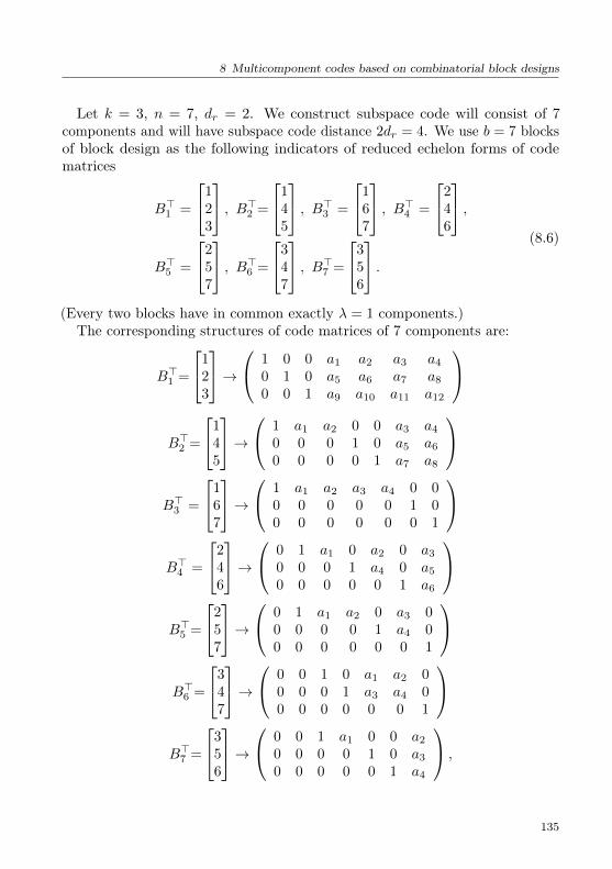
8 Multicomponent codes based on combinatorial block designs
Let k = 3, n = 7, dr = 2. We construct subspace code will consist of 7components and will have subspace code distance 2dr = 4. We use b = 7 blocksof block design as the following indicators of reduced echelon forms of codematrices
B>1 =
123
, B>2 =
145
, B>3 =
167
, B>4 =
246
,B>5 =
257
, B>6 =
347
, B>7 =
356
.(8.6)
(Every two blocks have in common exactly λ = 1 components.)The corresponding structures of code matrices of 7 components are:
B>1 =
123
→ 1 0 0 a1 a2 a3 a4
0 1 0 a5 a6 a7 a8
0 0 1 a9 a10 a11 a12
B>2 =
145
→ 1 a1 a2 0 0 a3 a4
0 0 0 1 0 a5 a6
0 0 0 0 1 a7 a8
B>3 =
167
→ 1 a1 a2 a3 a4 0 0
0 0 0 0 0 1 00 0 0 0 0 0 1
B>4 =
246
→ 0 1 a1 0 a2 0 a3
0 0 0 1 a4 0 a5
0 0 0 0 0 1 a6
B>5 =
257
→ 0 1 a1 a2 0 a3 0
0 0 0 0 1 a4 00 0 0 0 0 0 1
B>6 =
347
→ 0 0 1 0 a1 a2 0
0 0 0 1 a3 a4 00 0 0 0 0 0 1
B>7 =
356
→ 0 0 1 a1 0 0 a2
0 0 0 0 1 0 a3
0 0 0 0 0 1 a4
,
135

8 Multicomponent codes based on combinatorial block designs
where ai denotes free parameters.Here we used a balanced incomplete block design with parameters n = v =
b = 7, r = K = 3, λ = 1. The blocks Bi of the design above serve as theindicators for the 7 base matrices for the 7 components. Next, we will fillcolumns of matrices with free elements by columns of restricted rank code. Thisallows us to construct the required subspace code with subspace distance 4 as aunion of the 7 component codes of cardinalities 256, 16, 1, 16, 2, 4, 2 respectively.
The rank code distance of every component code will be at least dr = 2, sincewe use restricted rank metric mother code with dr = 2. Hence, the subspacecode distance of every component code will be at least 2dr = 4. The minimumsubspace distance between components of the code will be 4. As a result, themulticomponent code has subspace distance 4 and 297 code words, which is16% more than the cardinality of the first component.
Below we will show code matrices of the first two components of the code.
8.5.1 Matrices of the first and the second components
Matrices of the first component code. In the example above, the firstcomponent of the multicomponent code coincides with the SKK code. Let usconstruct a code matrix of the subspace code for a given information vector.
The parameters of the rank code are q = 2, dr = 2, k = n−dr+1 = 3−2+1 =2.
To design the extension field select the primitive polynomial f(λ) = λ4 +λ+1.The generator matrix of the rank code is
G =
[1 α α2
1 α2 α4
]. (8.7)
For information vector (u1, u2) compute the code vector
g = (u1, u2)G = ((u1 + u2), (u1α+ u2α2), (u1α
2 + u2α4)) = (g1, g2, g3).
Let the information symbols be u1 = α, u2 = α2. Then the code vector isg = (α5, α10, α2) and the code matrix is
M1 =
0 1 01 1 01 1 10 0 0
,
136

8 Multicomponent codes based on combinatorial block designs
with the transposed matrix
MT1 =
0 1 1 01 1 1 00 0 1 0
.Using lifting we obtain the basis of the code subspace as rows of the matrixX1 = [I3 MT
1 ]
X1 =
1 0 0 0 1 1 00 1 0 1 1 1 00 0 1 0 0 1 0
.The first component has 28 = 256 code matrices.
Matrices of the second component code. The code parameters andthe generator matrix are the same for all components: q = 2, dr = 2, k =n− dr + 1 = 3− 2 + 1 = 2.The indicator for the second component is
B2=[1 4 5] (8.8)
and the code matrices of the second component have the following structure
X2 =
1 a11 a12 0 0 a13 a14
0 0 0 1 0 a23 a24
0 0 0 0 1 a33 a34
, (8.9)
hence, the structure of a code matrix of the restricted rank code is
M1 =
a11 0 0a12 0 0a13 a23 a33
a14 a24 a34
. (8.10)
Here we have 8 free elements a11, a12, a13, a14, a23, a24, a33, a34. Four positionsare filled by zeros a21 = 0, a22 = 0, a31 = 0, a32 = 0. These are restrictions. Letus design all the code matrices and all the allowed information vectors.We use 1, α, α2, α3 as a basis of the extension field. Transform the second
and the third columns of the matrix into elements g2 and g3 of the extensionfield. Using, G, we obtain for information symbols u1, u2 the following systemof equations
137
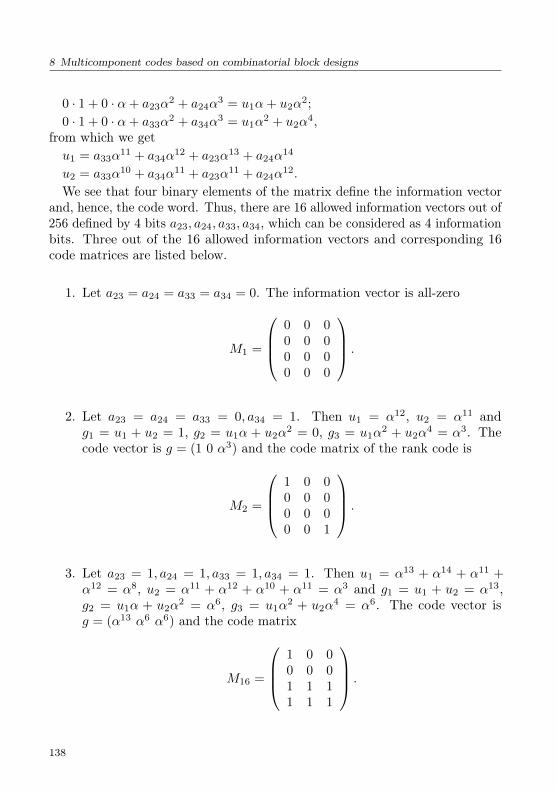
8 Multicomponent codes based on combinatorial block designs
0 · 1 + 0 · α+ a23α2 + a24α
3 = u1α+ u2α2;
0 · 1 + 0 · α+ a33α2 + a34α
3 = u1α2 + u2α
4,from which we getu1 = a33α
11 + a34α12 + a23α
13 + a24α14
u2 = a33α10 + a34α
11 + a23α11 + a24α
12.We see that four binary elements of the matrix define the information vector
and, hence, the code word. Thus, there are 16 allowed information vectors out of256 defined by 4 bits a23, a24, a33, a34, which can be considered as 4 informationbits. Three out of the 16 allowed information vectors and corresponding 16code matrices are listed below.
1. Let a23 = a24 = a33 = a34 = 0. The information vector is all-zero
M1 =
0 0 00 0 00 0 00 0 0
.
2. Let a23 = a24 = a33 = 0, a34 = 1. Then u1 = α12, u2 = α11 andg1 = u1 + u2 = 1, g2 = u1α + u2α
2 = 0, g3 = u1α2 + u2α
4 = α3. Thecode vector is g = (1 0 α3) and the code matrix of the rank code is
M2 =
1 0 00 0 00 0 00 0 1
.
3. Let a23 = 1, a24 = 1, a33 = 1, a34 = 1. Then u1 = α13 + α14 + α11 +α12 = α8, u2 = α11 + α12 + α10 + α11 = α3 and g1 = u1 + u2 = α13,g2 = u1α + u2α
2 = α6, g3 = u1α2 + u2α
4 = α6. The code vector isg = (α13 α6 α6) and the code matrix
M16 =
1 0 00 0 01 1 11 1 1
.
138

8 Multicomponent codes based on combinatorial block designs
8.6 Decoding a restricted rank code
Let us consider the decoding of the restricted rank code used in the secondcomponent. Since the restricted code is a subcode of the mother rank code, wecan decode the received word by decoding the mother code using any knowndecoding algorithm.
Assume the code matrix M16 has been transmitted over a noisy channel thatadds the following noise matrix of rank 1
Mn =
0 0 00 0 01 1 11 1 1
.
The received corrupted matrix is
Y =
1 0 00 0 00 0 00 0 0
.
To start decoding we transform the received matrix to the vector form y = (1 0 0).Using the generator matrix (8.3), let us compute a check matrix
H =
h1
h2
h3
.
Since the generator matrix is orthogonal to a check matrix we write GHT = 0as (
1 α α2
1 α2 α4
) h1
h2
h3
=
(00
)(8.11)
and obtain the system of equations for elements of the matrix H
h1 + αh2 + α2h3 = 0, h1 + α2h2 + α4h3 = 0. (8.12)
Setting h1 = 1 we find h2 = α2 and h3 = α12.
139

8 Multicomponent codes based on combinatorial block designs
The syndrome of the received vector is S = yHT , i.e.,
S = (1 0 0)
1α2
α12
= 1. (8.13)
Since the syndrome is nonzero we can detect an error during the transmission.The restricted code has code distance dr = 2 like the mother code, and candetect errors but cannot correct them.
8.7 Decoding subspace code
Let us use the following matrix of restricted rank code
M16 =
1 0 00 0 01 1 11 1 1
to build the code matrix X16 of the second component, having the indicatorB = [1 4 5]:
X16 =
1 1 0 0 0 1 10 0 0 1 0 1 10 0 0 0 1 1 1
. (8.14)
Assume that the rows of the matrix X16 were transmitted as packets via anetwork with linear random network coding and the matrix received is
Y = AX16. (8.15)
Let the matrix A in our example be the singular matrix
A =
1 0 10 1 01 1 1
(8.16)
140

8 Multicomponent codes based on combinatorial block designs
then the received matrix is
Y = AX16 =
1 0 10 1 01 1 1
1 1 0 0 0 1 10 0 0 1 0 1 10 0 0 0 1 1 1
= 1 1 0 0 1 0 00 0 0 1 0 1 11 1 0 1 1 1 1
.
(8.17)
Transform the matrix Y to the reduced row echelon form
Y =
1 1 0 0 1 0 00 0 0 1 0 1 10 0 0 0 0 0 0
. (8.18)
The positions of leading elements in the first two rows of the matrix Y allow usto find two columns of the identity matrix: the first and the forth. The fifthcolumn can be found using indicators. As a result, we have the positions ofindicators 1, 4, 5. Fixing the positions 1, 4, 5 of the component indicators, allowsus to find the channel matrix A from Y . Let us write A = I + L, where
L =
0 0 10 0 00 0 1
. (8.19)
The unindexed columns of the matrix Y form the matrix AM16
AM16 = M16 + LM16 =
1 0 0 00 0 1 10 0 0 0
. (8.20)
Write the transposed matrices
MT16 +MT
16LT =
1 0 00 0 00 1 00 1 0
(8.21)
and
LT =
0 0 00 0 01 0 1
. (8.22)
141

8 Multicomponent codes based on combinatorial block designs
Transform the matrix MT16 into a vector, denoted by (m1 m2 m3). Multiply the
vector by the matrix LT : (m1 m2 m3)LT = (m3 0 m3). Write the syndromeusing the unknown m3 as
S1 = m3(1 0 1)
1α2
α12
= m3(1 + α12) = m3α11. (8.23)
Transform the matrix MT16 into the vector y = (1 α6 0) and compute the
syndrome
(1 α6 0)
1α2
α12
= 1 + α8 = α2. (8.24)
By equating the expressions for the syndrome we obtain m3α11 = α2, i.e.,
m3 = α6. Error in vector form is e = (m3 0 m3) = (α6 0 α6). The transmittedvector is y + e = (1 + α6 α6 α6) = (α13 α6 α6) and corresponding decodedmatrix is
M16 =
1 0 00 0 01 1 11 1 1
. (8.25)
The decoding was correct.
Construction of a code with 13 components
Let us use a block design with parameters n = v = b = 13, r = K = 4, λ = 1from Table 1 in [Hal67] to construct a multicomponent subspace code withsubspace distance 2dr = 6, where code binary matrices have size n × r. Therows of the following table, which are blocks of the code design, will be used asindicators for 13 components. Here every row and every column has 4 differentpositions.Table of indicators (rows) of 13 components
142

8 Multicomponent codes based on combinatorial block designs
1 2 3 41 5 6 71 8 9 101 11 12 13
2 5 8 112 6 9 122 7 10 13
3 5 9 133 6 10 113 7 8 12
4 5 10 124 6 8 134 7 9 11
As an example let us show structures of code matrices of the second and thethirteens components of the subspace code.A code matrix of the second component has the following structure
1 a a a 0 0 0 a a a a a a0 0 0 0 1 0 0 a a a a a a0 0 0 0 0 1 0 a a a a a a0 0 0 0 0 0 1 a a a a a a
.
A code matrix of the 13-th component has the following structure0 0 0 1 a a 0 a 0 a 0 a a0 0 0 0 0 0 1 a 0 a 0 a a0 0 0 0 0 0 0 0 1 a 0 a a0 0 0 0 0 0 0 0 0 0 1 a a
.
Symbols a denote free elements. These free positions can be filled by elementsof a code word of the restricted [13, 11, 3] rank metric code over the extensionfield F24 .The number of code words in this subspace code with 13 components and
subspace distance 6 is 218+212+26+20+26+24+22+23+24+25+23+24+25 =266501. Using this multicomponent construction we increase the cardinality ofthe first component, which is the SKK code of cardinality 218 = 262144, by lessthan 2%. However, the multicomponent code has 4357 additional code words.
143

8 Multicomponent codes based on combinatorial block designs
8.8 Conclusions
We have developed the principles for building multicomponent subspace codesusing combinatorial block designs and rank codes. The required parametershave been selected in such a way that the minimum subspace distances betweenthe code components are not less than the code distance of the components.We have also elaborated the rank codes with restriction, which are required forthe multicomponent codes.
144
9Problems
9.1 Subgroups
Problem 1.
1. Find all subgroups of the additive group of the ring Z30. Specify whichsubgroups are cyclic and give generator elements for them.
2. Find the maximal multiplicative group of the ring Z30 and give all sub-groups of the group.
Solution
1. An operation of addition in additive group of the ring Z30 is the additionmodulo 30. The group is cyclic and consists of elements 0, 1, 2, . . . , 28, 29with the generator element 1. The order of the group is 30. Orders ofsubgroups should divide 30, i.e., the orders are 1, 2, 3, 5, 6, 10, 15, 30.The subgroup of order 1 consists of one element 0. The subgroup of order 2(which is cyclic with the generator element 15) consists of elements 0, 15.The subgroup of order 3 (which is cyclic with the generator element 10)consists of elements 0, 10, 20. The subgroup of order 5 (which is cyclicwith the generator element 6) consists of elements 0, 6, 12, 18, 24. Thesubgroup of order 6 (which is cyclic with the generator element 5) consists
145

9 Problems
of elements 0, 5, 10, 15, 20, 25. The subgroup of order 10 (which is cyclicwith the generator element 3) consists of elements 0, 3, 6, 9, 12, 15, 20, 25.The subgroup of order 15 (which is cyclic with the generator element 2)consists of elements 0, 2, 2, 4, 6, 8, 10, 12, 14, 16, 18, 20, 22, 24, 26, 28.
2. An operation of multiplication in the ring Z30 is the multiplication modulo30. The maximal multiplicative group consists of all elements that areco-prime with the module 30. These are 1, 7, 11, 13, 17, 19, 23, 29. Theorder of the group is 8. The group is not cyclic. Orders of subgroupsshould divide 8, i.e., the orders are 1, 2, 4, 8. The subgroup of order1 consists of one element 1. There are 3 different subgroups of order 2.These are: the cyclic subgroup 1, 11 with the generator element 11; thecyclic subgroup 1, 19 with the generator element 19; the cyclic subgroup1, 29 with the generator element 29. The are 3 different subgroups oforder 4. These are: the cyclic subgroup 1, 7, 19, 13 with the generatorelement 7; the cyclic subgroup 1, 17, 19, 23 with the generator element17; the subgroup 1, 11, 19, 29 (which is the product of two differentsubgroups of order 2 with the generator elements 11 and 19).
Problem 2.
1. Find all subgroups of the additive group of the ring Z19 and specify thegenerator elements for the subgroups.
2. Show that the maximal multiplicative group of the ring Z19 is cyclic andfind all the generator elements. Give all subgroups of the group.
Solution
1. An operation of addition in the additive group of the ring Z19 is theaddition modulo 19. The group is cyclic and consists of the elements0, 1, 2, . . . , 17, 18. A generator element is any nonzero element of thegroup. Since the order 19 of the group is prime, there are two subgroups:the group itself and 0.
2. The operation of multiplication in the ring Z19 is the multiplicationmodulo 19. The maximal multiplicative group consists of all elementsthat are co-prime with the module 19. These are all nonzero elements1, 2, 3, . . . , 17, 18. The order of the group is 18. The order of the sub-group 18, 9, 6, 3, 2, 1 divides 18. The maximal group of order 18 is cyclic.
146

9 Problems
A generator element is, e.g., 2. Indeed, all 18 powers 2, 22, 23, . . . , 217, 218
are different modulo 18. Other generator elements are 3, 10, 13, 14, 15.The subgroup of order 9 is cyclic with the generator element 4. Thesubgroup of order 6 is cyclic with the generator element 8. The subgroupof order 3 is cyclic with the generator element 7. The subgroup of order2 is cyclic and consists of elements 18, 1. The subgroup of order 1 hasonly one element 1.
Problem 3.Find the greatest common divisor of the polynomials r1(x) and r2(x) in the
ring GF(2)[x].r1(x) = x7 + x5 + x4 + x3 + x,r2(x) = x14 + x12 + x8 + x6 + x5 + x4 + 1.
Solutionr(x) = x2 + x+ 1.
Problem 4.Find the greatest common divisor of the polynomials r1(x) and r2(x) in the
ring GF(2)[x], wherer1(x) = x10 + x9 + x7 + x6 + x5 + x2 + 1,r2(x) = x16 + x15 + x14 + x13 + x12 + x9 + x6 + x4 + x2 + x+ 1.
Solutionr(x) = x3 + x2 + 1.
9.2 Rank codes
Problem 1.Consider linearized polynomials r1 = αx + α4x2, r2 = α3x + α8x2 over
the field GF (24), generated by the irreducible polynomial x4 + x3 + 1. Findlinearized polynomials r1 + r2, r1 ∗ r2, r2 ∗ r1.
147

9 Problems
Problem 2.The check matrix of the rank code of length n = 3 with code distance d = 3
over GF (23) is
H =
[1 α α2
1 α2 α4
],
where α is a root of the polynomial ϕ(x) = x3 +x2 + 1. Find a generator matrixof the code.
Let a code word matrix V has been transmitted. Decode the received matrix
Y = V + E =
0 1 11 0 01 0 1
assuming that the error matrix E has rank 1.
Solution
1. Build the table of the field generted by x3 + x2 + 1:
0 1 = α0 α α2 α3 α4 α5 α6
0 1 α α2 1 + α2 1 + α+ α2 1 + α α+ α2 .
2. Find a generator matrix G =[g1 g2 g3
]using the equation
GH> = 0.
Let g1 = 1, then g2 = α3, g3 = α4, and
G =[1 α3 α4
].
3. Transform the matrix Y into the vector form:
Y = V + E =
0 1 11 0 01 0 1
⇒ y = v + e =[α6 1 α3
].
4. The error vector of rank 1 can be written as
e = e1
[u1 u2 u3
]= e1U,
where e1 ∈ GF (23), ui ∈ GF (2).
148
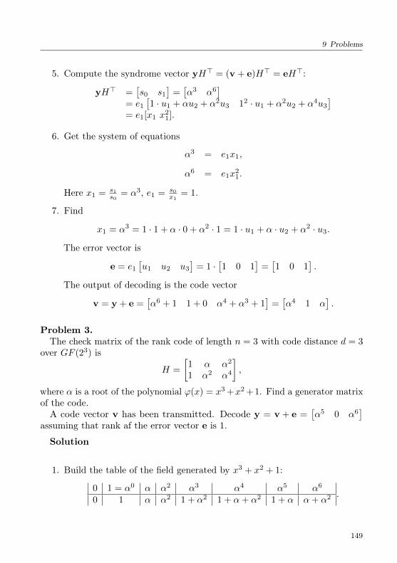
9 Problems
5. Compute the syndrome vector yH> = (v + e)H> = eH>:
yH> =[s0 s1
]=[α3 α6
]= e1
[1 · u1 + αu2 + α2u3 12 · u1 + α2u2 + α4u3
]= e1[x1 x
21].
6. Get the system of equations
α3 = e1x1,
α6 = e1x21.
Here x1 = s1s0
= α3, e1 = s0x1
= 1.
7. Find
x1 = α3 = 1 · 1 + α · 0 + α2 · 1 = 1 · u1 + α · u2 + α2 · u3.
The error vector is
e = e1
[u1 u2 u3
]= 1 ·
[1 0 1
]=[1 0 1
].
The output of decoding is the code vector
v = y + e =[α6 + 1 1 + 0 α4 + α3 + 1
]=[α4 1 α
].
Problem 3.The check matrix of the rank code of length n = 3 with code distance d = 3
over GF (23) is
H =
[1 α α2
1 α2 α4
],
where α is a root of the polynomial ϕ(x) = x3 +x2 + 1. Find a generator matrixof the code.A code vector v has been transmitted. Decode y = v + e =
[α5 0 α6
]assuming that rank af the error vector e is 1.
Solution
1. Build the table of the field generated by x3 + x2 + 1:
0 1 = α0 α α2 α3 α4 α5 α6
0 1 α α2 1 + α2 1 + α+ α2 1 + α α+ α2 .
149
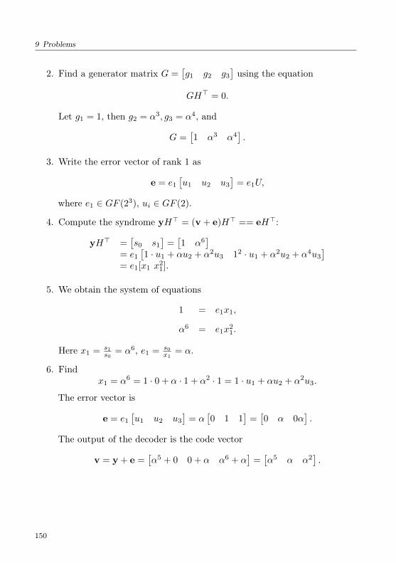
9 Problems
2. Find a generator matrix G =[g1 g2 g3
]using the equation
GH> = 0.
Let g1 = 1, then g2 = α3, g3 = α4, and
G =[1 α3 α4
].
3. Write the error vector of rank 1 as
e = e1
[u1 u2 u3
]= e1U,
where e1 ∈ GF (23), ui ∈ GF (2).
4. Compute the syndrome yH> = (v + e)H> == eH>:
yH> =[s0 s1
]=[1 α6
]= e1
[1 · u1 + αu2 + α2u3 12 · u1 + α2u2 + α4u3
]= e1[x1 x
21].
5. We obtain the system of equations
1 = e1x1,
α6 = e1x21.
Here x1 = s1s0
= α6, e1 = s0x1
= α.
6. Findx1 = α6 = 1 · 0 + α · 1 + α2 · 1 = 1 · u1 + αu2 + α2u3.
The error vector is
e = e1
[u1 u2 u3
]= α
[0 1 1
]=[0 α 0α
].
The output of the decoder is the code vector
v = y + e =[α5 + 0 0 + α α6 + α
]=[α5 α α2
].
150

9 Problems
Problem 4.The check matrix of the rank code of length n = 3 with code distance d = 3
over GF (23) is
H =
[1 α α2
1 α2 α4
],
where α is a root of the polynomial ϕ(x) = x3 +x2 + 1. Find a generator matrixof the code.A code vector v has been transmitted.
Decode y = v + e =[α3 1 0
]assuming that the rank of error vector e is 1.
Solution
1. Build the table of the field generated by x3 + x2 + 1:
0 1 = α0 α α2 α3 α4 α5 α6
0 1 α α2 1 + α2 1 + α+ α2 1 + α α+ α2 .
2. Find a generator matrix G =[g1 g2 g3
]using the equation
GH> = 0.
Let g1 = 1, then g2 = α3, g3 = α4, and
G =[1 α3 α4
].
3. The error vector of rank 1 write as
e = e1
[u1 u2 u3
]= e1U,
where e1 ∈ GF (23), ui ∈ GF (2).
4. Compute the syndrome yH> = (v + e)H> = eH>:
yH> =[s0 s1
]=[1 α6
]= e1
[1 · u1 + αu2 + α2u3 12 · u1 + α2u2 + α4u3
]= e1[x1 x
21].
5. Obtain the system of equations
1 = e1x1,
α6 = e1x21.
Here x1 = s1s0
= α6, e1 = s0x1
= α.
151

9 Problems
6. Find
x1 = α6 = 1 · 0 + α · 1 + α2 · 1 = 1 · u1 + αu2 + α2u3.
The error vector is
e = e1
[u1 u2 u3
]= α
[0 1 1
]=[0 α 0α
].
The output of the decoder is the code vector
v = y + e =[α5 + 0 0 + α α6 + α
]=[α5 α α2
].
9.3 q-cyclic codes
Problem 1.Let q = 2, m = 3. Consider the ring of linearized polynomials over the field
Fqm = F8. Let α be a primitive element of the field that satisfies α3 +α+ 1 = 0.Let us write the binomial xq
3 − x as xq3 − x = H1 ⊗ G1, where H1(x) =
xq + αx, G1(x) = xq2
+ α4xq + α6x. Factorize the binomial x[12] − x as follows
x[12] − x = (xq3 − x)⊗ (xq
3 − x)⊗ (xq3 − x)⊗ (xq
3 − x)= H1 ⊗G1 ⊗H1 ⊗G1 ⊗H1 ⊗G1 ⊗H1 ⊗G1
= H1 ⊗G1 ⊗H1 ⊗G1 ⊗H1 ⊗H1 ⊗G1 ⊗G1
= H ⊗G,
whereH = H1 ⊗G1 ⊗H1 ⊗G1 ⊗H1 ⊗H1,
G = G1 ⊗G1 = xq4
+αxq3
+xq2
+α5xq+α5x.
Build a q-cyclic code of length 12, then a 3-shortened q-cyclic code. Usingthis code build a 6-shortened q-cyclic code that is also a pseudo-cyclic code.
SolutionLet us build a q-cyclic code of length 4m = 12 using the polynomial G(x). A
152

9 Problems
generator matrix of the code is as follows
G =
α5 α5 1 α 1 0 0 0 0 0 0 00 α3 α3 1 α2 1 0 0 0 0 0 00 0 α6 α6 1 α4 1 0 0 0 0 00 0 0 α5 α5 1 α 1 0 0 0 00 0 0 0 α3 α3 1 α2 1 0 0 00 0 0 0 0 α6 α6 1 α4 1 0 00 0 0 0 0 0 α5 α5 1 α 1 00 0 0 0 0 0 0 α3 α3 1 α2 1
.
By deleting the last three rows and the last three columns in the matrix G weobtain a generator matrix G1 of 3-shortened q-cyclic code of length 3m = 9:
G1=
α5 α5 1 α 1 0 0 0 00 α3 α3 1 α2 1 0 0 00 0 α6 α6 1 α4 1 0 00 0 0 α5 α5 1 α 1 00 0 0 0 α3 α3 1 α2 1
.
This code is also a pseudo-q-cyclic code of length 3m = 9, generated by thesame polynomial G(x) in the factor-ring Lm(f1(x))[x] = Rm[x]/f1(x), where
f1(x) = (xq3−x)⊗ (xq
3−x)⊗ (xq3−x)
= x[9]+x[6]+xq3
+x.
By deleting the last three rows and the last three columns in the matrix G1 weobtain a generator matrix G2 of a 6-shortened q-cyclic code of length 6:
G2 =
(α5 α5 1 α 1 00 α3 α3 1 α2 1
).
This code is also a pseudo-q-cyclic code of length 2m = 6, generated by thesame polynomial G(x) in the factor-ring Lm(f2(x))[x] = Rm[x]/f2(x), where
f2(x) = (xq3−x)⊗ (xq
3−x)= x[6] + x.
This code is a q-cyclic code of length 6. In this problem, we analyzed sm-shortened q-cyclic codes for q = 2, m = 3, s = 4, s = 1, 2. However, if the
153
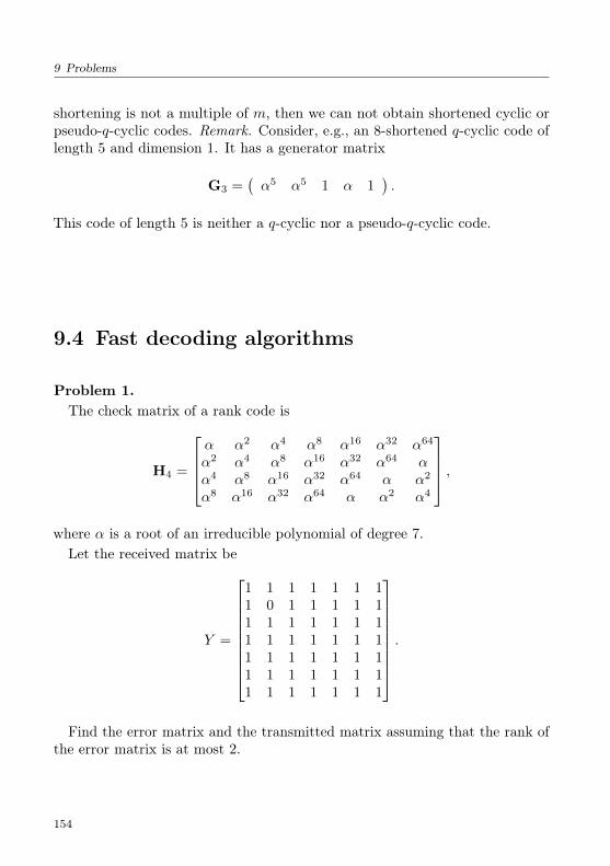
9 Problems
shortening is not a multiple of m, then we can not obtain shortened cyclic orpseudo-q-cyclic codes. Remark. Consider, e.g., an 8-shortened q-cyclic code oflength 5 and dimension 1. It has a generator matrix
G3 =(α5 α5 1 α 1
).
This code of length 5 is neither a q-cyclic nor a pseudo-q-cyclic code.
9.4 Fast decoding algorithms
Problem 1.The check matrix of a rank code is
H4 =
α α2 α4 α8 α16 α32 α64
α2 α4 α8 α16 α32 α64 αα4 α8 α16 α32 α64 α α2
α8 α16 α32 α64 α α2 α4
,where α is a root of an irreducible polynomial of degree 7.
Let the received matrix be
Y =
1 1 1 1 1 1 11 0 1 1 1 1 11 1 1 1 1 1 11 1 1 1 1 1 11 1 1 1 1 1 11 1 1 1 1 1 11 1 1 1 1 1 1
.
Find the error matrix and the transmitted matrix assuming that the rank ofthe error matrix is at most 2.
154

9 Problems
9.5 Symmetric rank codes
Problem 1.Find symmetric matrices that generate the fields F27 and F28 .
9.6 Rank codes in network coding
Problem 1.A subspace code X is defined by the set of base matrices
X =X : X =
[In M
],
where In is the identity matrix of order n, and M is an n × m matrix of amatrix codeM with a rank distance d. Find the subspace distance of the codeX .
9.7 Codes based on combinatorial block designs
Problem 1.Let the parameters of the block design be v = 9, n = b = 12, r = 4,K =
3, λ = 1. The i-th row of Table 9.1 gives indicators of the i-th component ofthe code. Design these 12 components and find their cardinalities.
155

9 Problems
Table 9.1: Table of indicators of 12 components1 2 3
4 5 67 8 9
1 4 72 5 8
3 6 91 5 9
2 6 73 4 8
1 6 82 4 9
3 5 7
Problem 2.Let the parameters of the block design be n = v = b = 13, r = K = 4, λ = 1.
The i-th row of Table 9.2 gives indicators of the i-th component of the code.
Table 9.2: Table of indicators of 13 components1 2 3 41 5 6 71 8 9 101 11 12 13
2 5 8 112 6 9 122 7 10 13
3 5 9 133 6 10 113 7 8 12
4 5 10 124 6 8 134 7 9 11
Design these 13 components and find their cardinalities.
156

Epilogue
This monograph presents the main results related to rank metric codes, obtainedso far by the author of the book and by other authors. It is shown that rankcodes can be successfully applied in multichannel communication systems, innetwork coding and for information protection against unauthorized use. Thework of the following authors deserves special attention: Kötter (Germany),Kschischang (Canada), and Silva (Brazil). Their joint works [KK08], [SKK08]in 2007-2008 created new subspace codes for random network coding. They usethe so-called lifting principle, where an identity matrix is concatenated with amatrix of a rank code as if the former matrix had lifted the letter up. Becauseof this principle, these codes are sometimes called lifted codes. The merit ofcreating these new codes, which are characterized by high cardinality, belongsentirely to these three authors. Following these authors, the works of Bossertand Gabidulin [GB08], [GB09] increased the power of these codes and broughtthem to the upper limit. Over a series of papers, these authors introduced andelaborated the concept of subspace multicomponent codes. Here, these resultsare presented.The theory of rank codes is developing successfully. New designs are being
created. The constructions of Kshevetskiy-Gabidulin [KG05] are among them.New rank codes have been published by Irish scientist Sheekey [She16]. Researchin this area is being carried out in Germany, Turkey, Switzerland and othercountries. It is generally agreed that the new codes can be used in cryptosystemsto increase security.
The development of rank coding theory is also reflected in a series of papersby Sidorenko with coauthors [SJB11], [LSS14], where the new codes are calledinterleaved rank metric codes. They improve the correcting ability of Gabidulincodes.
157


Bibliography
[ALR18] D. Augot, P. Loidreau, and G. Robert, “Generalized Gabidulincodes over fields of any characteristic,” Des. Codes Cryptogr.,vol. 86, no. 8, pp. 1807–1848, 2018.
[ANLY00] R. Ahlswede, Ning Cai, S. . R. Li, and R. W. Yeung, “Network in-formation flow,” IEEE Transactions on Information Theory, vol. 46,no. 4, pp. 1204–1216, 2000.
[Bar17] H. Bartz, “Decoding of subspace and rank-metric codes,” Ph.D.dissertation, Technical University of Munich, Munich, Germany,2017.
[Beu75] A. Beutelspacher, “Partial spreads in finite projective spaces andpartial designs,” Math. Z., vol. 145, pp. 211–229, 1975.
[BN06] A. Barg and D. Nogin, “Spectral approach to linear programmingbounds on codes,” Probl Inf Transm, vol. 42, pp. 77–89, 2006.
[BU09] D. Boucher and F. Ulmer, “Coding with skew polynomial rings,”Journal of Symbolic Computation, vol. 44, no. 12, pp. 1644–1656,2009.
[Cec84] P. Ceccherini, “ A q-analogous of the characterization of hypercubesas graphs,” J. of Geometry, vol. 22, pp. 57–74, 1984.
[Coo97] B. Cooperstein, “External flats to varieties in pg(mn,n(gf(q))),”Linear Algebra and its Applications, vol. 267, pp. 175 – 186, 1997.
[CW13] J. Cruz and W. Willems, “On network codes and partial spreads,”in Seventh International Workshop on Optimal Codes and RelatedTopics, Albena, Bulgaria, 2013, pp. 77–78.
159
Bibliography
[Del76] P. Delsarte, “Association schemes and t-designs in regularsemilattices,” Journal of Combinatorial Theory, Series A, vol. 20,no. 2, pp. 230 – 243, 1976.
[Del78] ——, “Bilinear Forms over a Finite Field, with Applications toCoding Theory,” Journal of Combinatorial Theory, Series A, vol. 25,no. 3, pp. 226–241, 1978.
[DF79] D. Drake and J. Freeman, “Partial t-spreads and group constructibles, r, µ-nets,” J. Geom., vol. 13, no. 2, pp. 210–216, 1979.
[ES09] T. Etzion and N. Silberstein, “Error-correcting codes in projectivespaces via rank-metric codes and Ferrers diagrams,” IEEE Transac-tions on Information Theory, vol. 55, no. 7, pp. 2909–2919, 2009.
[EZJS+10] S. El-Zanati, H. Jordon, G. F. Seelinger, P. Sissokho, and L. E.Spence, “The maximum size of a partial 3-spread in a finite vectorspace over GF(2),” Designs, Codes and Cryptography, vol. 54, pp.101–107, 2010.
[GA86] E. Gabidulin and V. Afanasyev, Coding in radio-electronics (inRussian). Moscow, Russia: Radio and Svyaz, 1986.
[Gab85] E. M. Gabidulin, “Theory of Codes with Maximum Rank Distance,”Probl. of Inform. Transm., vol. 21, no. 1, pp. 1–12, Jul 1985.
[Gab92] ——, “A fast matrix decoding algorithm for rank-error-correctingcodes,” in Algebraic Coding, G. Cohen, A. Lobstein, G. Zémor, andS. Litsyn, Eds. Berlin, Heidelberg: Springer Berlin Heidelberg,1992, pp. 126–133.
[Gan67] F. Gantmacher, The Theory of Matrices (in Russian). Nauka,Moscow, 1967.
[GB08] E. Gabidulin and M. Bossert, “Codes for network coding,” in Proc.ISIT, Toronto, Canada, 2008, pp. 867–870.
[GB09] ——, “A family of algebraic codes for network coding,” in Proc.ISIT, Seoul, Korea, 2009.
[GL08] E. Gabidulin and P. Loidreau, “Properties of subspace subcodes ofGabidulin codes,” Adv. Math. Commun., vol. 2, pp. 147–157, 2008.
160

Bibliography
[GOHA03] E. M. Gabidulin, A. V. Ourivski, B. Honary, and B. Ammar, “Re-ducible rank codes and their applications to cryptography,” IEEETransactions on Information Theory, vol. 49, no. 12, pp. 3289–3293,2003.
[GP02] E. Gabidulin and N. Pilipchuk, “Representation of a finite field bysymmetric matrices and applications,” in Proc. Eighth Int. Work-shop on Algebraic and Combinatorial Coding Theory, Tsarskoe Selo,Russia, 2002, pp. 120–123.
[GP04] ——, “Symmetric Rank Codes,” Problems of Information Transmis-sion, vol. 40, pp. 103–117, 2004.
[GP06] E. M. Gabidulin and N. I. Pilipchuk, “Symmetric matrices andcodes correcting rank errors beyond the (d− 1)/2 bound,” DiscreteApplied Mathematics, vol. 154, no. 2, pp. 305 – 312, 2006.
[GP08] ——, “Error and erasure correcting algorithms for rank codes,”Designs, Codes and Cryptography, vol. 49, no. 1, pp. 105–122, Dec2008.
[GP16] E. Gabidulin and N. Pilipchuk, “Multicomponent codes with max-imal code distance,” Probl. Inform. Transm., vol. 52, pp. 84–91,2016.
[GP17a] ——, “Cardinality of multicomponent zero prefix spreads,” in Pro-ceeding of Workshop on Coding and Cryptography, Moscow, Russia,2017.
[GP17b] ——, “Cardinality of subspace multicomponent codes,” in Proc. ofFourth International Conference on Engineering and Telecommuni-cations (En&T), Moscow, Russia, 2017, pp. 11–14.
[GPT92] E. Gabidulin, A. Paramonov, and O. Tretjakov, “Rank errors andrank erasures correcting,” in Proc.4th Int. Colloquium on CodingTheory, Dilijan, Yerevan, Armenia, 1992, pp. 11–19.
[GR92] E. M. Gabidulin and R. M. Roth, “Comments on "Maximum-rankarrays codes and their application to crisscross error correction"[with reply],” IEEE Transactions on Information Theory, vol. 38,no. 3, p. 1183, 1992.
161

Bibliography
[GR18] E. Gorla and A. Ravagnani, Codes Endowed with the Rank Metric.Cham: Springer International Publishing, 2018, pp. 3–23.
[GX12] V. Guruswami and C. Xing, “List Decoding Reed–Solomon,Algebraic-Geometric, and Gabidulin Subcodes up to the Single-ton Bound,” Electr. Colloq. Comp. Complexity, vol. 19, no. 146,2012.
[GY08] M. Gadouleau and Z. Yan, “Packing and covering properties of rankmetric codes,” IEEE Transactions on Information Theory, vol. 54,no. 9, pp. 3873–3883, 2008.
[Hal67] M. Hall, Combinatorial Theory, ser. Blaisdell book in pure andapplied mathematics. Wiley, 1967.
[HKK18] T. Honold, M. Kiermaier, and S. Kurz, “Partial spreads and vectorspace partitions,” Signals and Communication Technology, pp.131–170, 2018.
[HTR18] A.-L. Horlemann-Trautmann and J. Rosenthal, “Constructions ofconstant dimension codes,” in Network coding and subspace designs,ser. Signals and Communication Technology, M. Greferath, M. O.Pavčević, N. Silberstein, and M. Á. Vázquez-Castro, Eds. Cham:Springer, Januar 2018, pp. 25–42.
[Hua51] L.-K. Hua, “A theorem on matrices over a sfield and its applications,”Acta Mathematica Sinica, vol. 1, no. 2, pp. 109–163, 1951.
[KG05] A. Kshevetskiy and E. Gabidulin, “The new construction of rankcodes,” in Proceedings. International Symposium on InformationTheory, 2005. ISIT 2005., 2005, pp. 2105–2108.
[KK08] R. Koetter and F. Kschischang, “Coding for Errors and Erasuresin Random Network Coding,” Inform. Theory, IEEE Trans. on,vol. 54, no. 8, pp. 3579–3591, Aug. 2008.
[Kur16] S. Kurz, “Improved upper bounds for partial spreads,” Designs,Codes and Cryptography, vol. 85, no. 1, pp. 97–106, Oct 2016.
[Kur17] ——, “Packing vector spaces into vector spaces,” The AustralianJournal of Combinatorics, vol. 68, no. 1, pp. 122–130, March 2017.
162
Bibliography
[LGB03] P. Lusina, E. Gabidulin, and M. Bossert, “Maximum rank distancecodes as space-time codes,” IEEE Transactions on InformationTheory, vol. 49, no. 10, pp. 2757–2760, 2003.
[Li15] W. Li, “Decoding evaluation codes and their interleaving,” Ph.D.dissertation, University of Ulm, Ulm, Germany, 2015.
[LN83] R. Lidl and H. Niederreiter, Finite Fields, ser. Encyclopedia ofmathematics and its applications. Addison-Wesley, AdvancedBook Program/World Science Division, 1983.
[LO06] P. Loidreau and R. Overbeck, “Decoding rank errors beyond theerror correcting capability,” in Proc. Int. Workshop on Algebraicand Combinatorial Coding Theory, 2006, pp. 186–190.
[LSS14] W. Li, V. Sidorenko, and D. Silva, “On transform-domain errorand erasure correction by Gabidulin codes,” Designs, Codes andCryptography, vol. 73, pp. 571–586, 2014.
[LTZ18] G. Lunardon, R. Trombetti, and Y. Zhou, “Generalized twistedGabidulin codes,” Journal of Combinatorial Theory, Series A, vol.159, pp. 79–106, Oct 2018.
[Mar17] U. Martínez-Peñas, “On the roots and minimum rank distance ofskew cyclic codes,” Designs, Codes and Cryptography, vol. 83, no. 3,pp. 639–660, 2017.
[Moo96] E. Moore, “A two-fold generalization of Fermat’s theorem,” Bull.Amer. Math. Soc., vol. 2, no. 7, pp. 189–199, 04 1896.
[MV19] H. Mahdavifar and A. Vardy, “Algebraic list-decoding in projectivespace: Decoding with multiplicities and rank-metric codes,” IEEETransactions on Information Theory, vol. 65, no. 2, pp. 1085–1100,2019.
[Ner20] A. Neri, “Systematic encoders for generalized Gabidulin codesand the q-analogue of Cauchy matrices,” Linear Algebra and itsApplications, vol. 593, pp. 116–149, 2020.
[OÖ16] K. Otal and F. Özbudak, “Explicit constructions of some non-Gabidulin linear maximum rank distance codes,” Advances in Math-ematics of Communications, vol. 10, 2016.
163
Bibliography
[OÖ17] ——, “Additive rank metric codes,” IEEE Transactions on Informa-tion Theory, vol. 63, no. 1, pp. 164–168, 2017.
[PRLS17] S. Puchinger, J. Rosenkilde né Nielsen, W. Li, and V. Sidorenko,“Row Reduction Applied to Decoding of Rank-Metric and SubspaceCodes,” Designs, Codes and Cryptography, vol. 82, no. 1-2, pp.389–409, 2017.
[PRS17] S. Puchinger, J. Rosenkilde né Nielsen, and J. Sheekey, “Furthergeneralisations of twisted Gabidulin codes,” in Proceedings of Inter-national Workshop on Coding and Cryptography, 2017.
[Puc18] S. Puchinger, “Construction and decoding of evaluation codes inHamming and rank metric,” Ph.D. dissertation, University of Ulm,Ulm, Germany, 2018.
[Rot91] R. M. Roth, “Maximum-Rank Array Codes and their Applicationto Crisscross Error Correction,” IEEE Transactions on InformationTheory, vol. 37, no. 2, pp. 328–336, 1991.
[Sag10] Y. L. Sagalovich, Introduction to algebraic codes (in Russian). IITPRAS, Moscow, Russia, 2010.
[Seg64] B. Segre, “Teoria di Galois fibrazioni proettive e geometric nondesarguesiane,” Ann. Mat. pura appl., vol. 64, pp. 1–76, 1964.
[She16] J. Sheekey, “A new family of linear maximum rank distance codes,”Advances in Mathematics of Communications, vol. 10, pp. 475–488,2016.
[SJB11] V. Sidorenko, L. Jiang, and M. Bossert, “Skew-Feedback Shift-Register Synthesis and Decoding Interleaved Gabidulin Codes,” In-form. Theory, IEEE Trans. on, vol. 57, no. 2, pp. 621–632, Feb.2011.
[SKK08] D. Silva, F. Kschischang, and R. Koetter, “A Rank-Metric Approachto Error Control in Random Network Coding,” Inform. Theory,IEEE Trans. on, vol. 54, no. 9, pp. 3951–3967, Sep. 2008.
[SN17a] P. Sissokho and E. Nastase, “The maximum size of a partial spreadII: Upper bounds,” Discrete Math., vol. 340, pp. 1481–1487, 2017.
164
Bibliography
[SN17b] ——, “The maximum size of a partial spread in a finite projectivespace,” J.Combin.Theory Ser.A., vol. 152, pp. 122–130, 2017.
[WXSN03] H. Wang, C. Xing, and R. Safavi-Naini, “Linear authentication codes:bounds and constructions,” IEEE Transactions on InformationTheory, vol. 49, no. 4, pp. 866–872, 2003.
[WZ13] A. Wachter-Zeh, “Decoding of block and convolutional codes in rankmetric,” Ph.D. dissertation, University of Ulm, Ulm, Germany, 2013.
165